on a reformulated convolution quadrature based boundary element · pdf fileon a reformulated...

Copyright © 2010 Tech Science Press CMES, vol.58, no.2, pp.109-128, 2010

On a Reformulated Convolution Quadrature BasedBoundary Element Method

M. Schanz1

Abstract: Boundary Element formulations in time domain suffer from two prob-lems. First, for hyperbolic problems not too much fundamental solutions are avail-able and, second, the time stepping procedure is expensive in storage and has stabil-ity problems for badly chosen time step sizes. The first problem can be overcomeby using the Convolution Quadrature Method (CQM) for time discretisation. Thisas well improves the stability. However, still the storage requirements are large.A recently published reformulation of the CQM by Banjai and Sauter [Rapid solu-tion of the wave equation in unbounded domains, SIAM J. Numer. Anal., 47, 227–249] reduces the time stepping procedure to the solution of decoupled problems inLaplace domain. This new version of the CQM is applied here to elastodynam-ics. The storage is reduced to nearly the amount necessary for one calculation inLaplace domain. The properties of the original method concerning stability in timeare preserved. Further, the only parameter to be adjusted is still the time step size.The drawback is that the time history of the given boundary data has to be knownin advance. These conclusions are validated by the examples of an elastodynamiccolumn and a poroelastodynamic half space.

Keywords: BEM, time domain, CQM

1 Introduction

The Boundary Element Method (BEM) in time domain is especially import to treatwave propagation problems in infinite and semi-infinite domains. In this applica-tion the main advantage of this method becomes obvious, i.e., its ability to modelthe Sommerfeld radiation condition correctly. Certainly this is not the only ad-vantage of a time domain BEM but very often the main motivation as, e.g., inearthquake engineering.

The first boundary integral formulation for elastodynamics was published by Cruseand Rizzo (1968). This formulation performs in Laplace domain with a subsequent1 Graz University of Technology, Institute of Applied Mechanics

110 Copyright © 2010 Tech Science Press CMES, vol.58, no.2, pp.109-128, 2010

inverse transformation to time domain to achieve results for the transient behav-ior. The corresponding formulation in Fourier domain, i.e., frequency domain, waspresented by Domínguez (1978). The first boundary element formulation directlyin the time domain was developed by Mansur for the scalar wave equation andfor elastodynamics with zero initial conditions (Mansur, 1983). The extension ofthis formulation to non-zero initial conditions was presented by Antes (1985). De-tailed information about this procedure may be found in the book of Domínguez(1993). A comparative study of these possibilities to treat elastodynamic problemswith BEM was given by Manolis (1983). A completely different approach to han-dle dynamic problems utilizing static fundamental solutions is the so-called dualreciprocity BEM. This method was introduced by Nardini and Brebbia (1982) anddetails may be found in the monograph of Partridge, Brebbia, and Wrobel (1992).A very detailed review on elastodynamic boundary element formulations and a listof applications can be found in two articles of Beskos (1987, 1997).

The above listed methodologies to treat elastodynamic problems with the BEMshow mainly the two ways: direct in time domain or via an inverse transformationin Laplace domain. Mostly, the latter is used, e.g., Ahmad and Manolis (1987).Since all numerical inversion formulas depend on a proper choice of their param-eters (Narayanan and Beskos, 1982), a direct evaluation in time domain seems tobe preferable. Also, it is more natural to work in the real time domain and observethe phenomenon as it evolves. But, as all time-stepping procedures, such a formu-lation requires an adequate choice of the time step size. An improper chosen timestep size leads to instabilities or numerical damping. Four procedures to improvethe stability of the classical dynamic time-stepping BE formulation can be quoted:the first employs modified numerical time marching procedures, e.g., Antes andJäger (1995) for acoustics, Peirce and Siebrits (1997) for elastodynamics; the sec-ond employs a modified fundamental solution, e.g., Rizos and Karabalis (1994)for elastodynamics; the third employs an additional integral equation for veloci-ties (Mansur, Carrer, and Siqueira, 1998); and the last uses weighting methods,e.g., Yu, Mansur, Carrer, and Gong (1998) for elastodynamics and Yu, Mansur,Carrer, and Gong (2000) for acoustics.

Beside these improved approaches there exist the possibility to solve the convo-lution integral in the boundary integral equation with the so-called ConvolutionQuadrature Method (CQM) proposed by Lubich (1988a,b). Applications to hyper-bolic and parabolic integral equations can be found in Lubich and Schneider (1992);Lubich (1994). The CQM utilizes the Laplace domain fundamental solution and re-sults not only in a more stable time stepping procedure but also damping effects incase of visco- or poroelasticity can be taken into account (see Schanz and Antes(1997a,b); Schanz (2001a)). The motivation to use the CQM in these engineering

Reformulated CQM BEM 111

applications is that only the Laplace domain fundamental solutions are required.This fact is also used for BE formulations in cracked anisotropic elastic (Zhang,2000) or piezoelectric materials (García-Sánchez, Zhang, and Sáez, 2008). Anotheraspect is the better stability behavior compared with the above mentioned formula-tion. For acoustics this may be found in Abreu, Carrer, and Mansur (2003); Abreu,Mansur, and Carrer (2006) and in elastodynamics in Schanz (2001b). In the frame-work of fast BE formulations the CQM is used in a Panel-clustering formulation forthe Helmholtz equation by Hackbusch, Kress, and Sauter (2007). Recently, somenewer mathematical aspects of the CQM have been published by Lubich (2004).

Important for the paper at hand, an essential reformulation of the CQM in caseof integral equations has been published by Banjai and Sauter (2009). The pro-posed formulation transfers the time stepping procedure to the solution of decou-pled Laplace domain problems. The main parameter of the method is still theapplied time step size. In this paper, some stability proofs with respect to the timedependent behavior can be found. Here, this technique is applied to elastodynamicsfor a collocation and a symmetric Galerkin formulation. At the end some numeri-cal studies are performed concerning the sensitivity on the mesh size, the time stepsize, and on the precision of the equation solver. To show the applicability of thereformulated CQM to inelastic BE formulations the displacement results for wavepropagation in a poroelastic half space are presented.

Throughout this paper, vectors and tensors are denoted by bold symbols and matri-ces by sans serif and upright symbols. The Laplace transform of a function f (t) isdenoted by f (s) with the complex Laplace parameter s.

2 Boundary integral equation

The hyperbolic partial differential equation to be considered in this work is theelastodynamic system, which describes the displacement field u(x, t) of an elasticsolid under the assumptions of linear elasticity. Describing with x and t the positionin the three-dimensional Euclidean space R3 and the time point from the interval(0,∞) the hyperbolic initial boundary value problem is

c21∇(∇ ·u(x, t))− c2

2∇× (∇×u(x, t)) =∂ 2u∂ t2 (x, t) (x, t) ∈Ω× (0,∞)

u(y, t) = gD(y, t) (y, t) ∈ ΓD× (0,∞)t(y, t) = gN(y, t) (y, t) ∈ ΓN× (0,∞)

u(x,0) =∂u∂ t

(x,0) = 0 (x, t) ∈Ω× (0) .

(1)


The material properties of the solid are represented by the wave speeds

c1 =

√E (1−ν)

ρ (1−2ν)(1+ν)c2 =

√E

ρ2(1+ν), (2)

with the material data Young’s modulus E, Poisson’s ration ν , and the mass den-sity ρ . The first statement in (1) requires the fulfillment of the partial differentialequation in the spatial domain Ω for all times 0 < t < ∞. This spatial domain Ω

has the boundary Γ which is subdivided into two disjoint sets ΓD and ΓN at whichboundary conditions are prescribed. The Dirichlet boundary condition is the secondstatement of (1) and assigns a given datum gD to the displacement u on the part ΓD

of the boundary. Similarly, the Neumann boundary condition is the third statementin which the datum gN is assigned to the surface traction t, which is defined by

t(y, t) = (T u)(y, t) = limΩ3x→y∈Γ

[σσσ(x, t) ·n(y)] . (3)

In (3), σσσ is the stress tensor depending on the displacement field u according to thestrain-displacement relationship and Hooke’s law. For later purposes the tractionoperator T is defined, which maps the displacement field u to the surface tractiont. The boundary conditions have to hold for all times and may be also prescribed ineach direction by different types, e.g., roller bearings. Finally, in the last statementof (1) the condition of a quiescent past is given which implies homogeneous initialconditions.

The representation formula may be derived from the dynamic reciprocal iden-tity (Wheeler and Sternberg, 1968) or also from a weighted residual statement.With the Riemann convolution defined as

(g∗h)(x, t) =∫ t

0g(x, t− τ)h(τ)dτ , (4)

and the fundamental solution U(x−y, t− τ) of equation (1) the representation for-mula

u(x, t) =∫ t

0

∫Γ

U(x−y, t− τ)t(y,τ)dsy dτ−∫ t

0

∫Γ

(TyU)(x−y, t− τ)u(y,τ)dsy dτ x ∈Ω,y ∈ Γ (5)

is given. Here, the surface measure dsy carries its subscript in order to emphasizethat the integration variable is y. Similarly, Ty indicates that the derivatives involvedin the computation of the surface traction due to equation (3) are taken with respectto the variable y. Explicit expressions for the used fundamental solutions can be


found, for instance, in Kausel (2006). By means of equation (5), the unknown u isgiven at any point x inside the domain Ω and at any time 0 < t < ∞, if the boundarydata u(y,τ) and t(y,τ) are known for all points y of the boundary Γ and times0 < τ < t.

The first boundary integral equation is obtained by taking expression (5) to theboundary. Using operator notation, this boundary integral equation reads

(V ∗ t)(x, t) = C(x)u(x, t)+(K∗u)(x, t) (x, t) ∈ Γ× (0,∞) . (6)

The introduced operators are the single layer operator V , the integral-free term C,and the double layer operator K which are defined as

(V ∗ t)(x, t) =∫ t

0

∫Γ

U(x−y, t− τ)t(y,τ)dsy dτ (7a)

C(x) = I+ limε→0

∫∂Bε (x)∩Ω

(TyU)>(x−y,0)dsy (7b)

(K∗u)(x, t) = limε→0

∫ t

0

∫Γ\Bε (x)

(TyU)>(x−y, t− τ)u(y,τ)dsy dτ . (7c)

In these expressions, Bε(x) denotes a ball of radius ε centered at x and ∂Bε(x) is itssurface. Note that the single layer operator (7a) involves a weakly singular integraland the double layer operator (7c) has to be understood in the sense of a principalvalue.

Application of the traction operator Tx to the dynamic representation formula (5)yields the second boundary integral equation

(D∗u)(x, t) = (I −C(x)) t(x, t)− (K′ ∗ t)(x, t) x ∈ Γ . (8)

The newly introduced operators are the adjoint double layer operator K′ and thehyper-singular operator D. They are defined as

(K′ ∗ t)(x, t) = limε→0

∫ t

0

∫Γ\Bε (x)

(TxU)(x−y, t− τ)t(y,τ)dsy dτ (9a)

(D∗u)(x, t) =− limε→0

∫ t

0Tx

∫Γ\Bε (x)

(TyU)>(x−y, t− τ)u(y,τ)dsy dτ . (9b)

The hyper-singular operator has to be understood in the sense of a finite part.

For the solution of mixed initial boundary value problems of the form (1), a non-symmetric formulation by means of the first boundary integral equation (6) in com-bination with a collocation technique will be used. A symmetric formulation is ob-tained using both the first and the second boundary integral equation, (6) and (8).


Symmetric formulation First, the Dirichlet datum u and the Neumann datum tare decomposed into

u = u+ gD and t = t+ gN , (10)

with arbitrary but fixed extensions, gD and gN , of the given Dirichlet and Neumanndata, gD and gN . They are introduced such that

gD(x, t) = gD(x, t) , (x, t) ∈ ΓD× (0,∞)gN(x, t) = gN(x, t) , (x, t) ∈ ΓN× (0,∞)

(11)

holds. The extension gD of the given Dirichlet datum has to be continuous due toregularity requirements (Steinbach, 2008).

In order to establish a symmetric formulation, the first boundary integral equation(6) is used only on the Dirichlet boundary ΓD whereas the second one (8) is usedonly on the Neumann part ΓN . Taking the prescribed boundary conditions (1) intoaccount and inserting the decompositions (10) into both integral equations leads tothe symmetric formulation for the unknowns u and t

V ∗ t−K∗ u = fD, (x, t) ∈ ΓD× (0,∞)D∗ u+K′ ∗ t = fN , (x, t) ∈ ΓN× (0,∞)

(12)

with the abbreviations

fD = CgD +K∗ gD−V ∗ gN

fN = (I −C) gN−K′ ∗ gN−D∗ gD .(13)

3 Boundary element formulation

A boundary element formulation is derived following the usual procedure.

3.1 Semi-discrete equations

Let the boundary Γ of the considered domain be represented in the computation byan approximation Γh which is the union of geometrical elements

Γh =Ne⋃

e=1

τe . (14)

τe denote boundary elements, e.g., surface triangles as in this work, and their totalnumber is Ne. Now, the boundary functions u and t are approximated with shapefunctions ϕi or ψ j, which are defined with respect to the geometry partitioning (14),


and time dependent coefficients uik and t j

k . This yields for the k-th component of thedata

uk(y, t) =N

∑i=1

uik(t)ϕi(y) and tk(y, t) =

M

∑j=1

t jk (t)ψ j(y) . (15)

Inserting these spatial shape functions in the boundary integral equations (12) and(6), respectively, and applying on the first a Galerkin scheme and on the latter a col-location method, results in the two semi-discrete equation systems. The Galerkinmethod with (12) yields[

V −KKT D

]∗[tu

]=[fDfN

](16)

and the collocation method yields for the first integral equation (6)

V ∗ t = Cu+K∗u . (17)

In the equations (16) and (17), the time is still continuous and the convolution hasto be performed. Further, the notation of matrices/vectors with sans serif lettersdenotes that in these matrices the data at all nodes and all degrees of freedom arecollected.

3.2 Convolution Quadrature Method

Next, the temporal discretization by the CQM has to be introduced. Its basic idea isto approximate the convolution integral (4) by a quadrature formula on an equidis-tant time grid of step size ∆t, i.e., 0 = t0 < ∆t = t1 < · · ·< n∆t = tn,

(g∗h)(x, tn)≈n

∑k=0

ωn−k(∆t,γ, g) f (k∆t) . (18)

In this expression, the quadrature weights ωn−k depend on the step size ∆t, thequotient of the characteristic polynomials γ of the underlying A-stable multistepmethod, and the Laplace transformed function g. The quadrature weights are com-puted following

ωn−k(∆t,γ, g) =R−(n−k)

L

L−1

∑`=0

g(s`)ζ−(n−k)`

ζ = e2πiL

with the complex ’frequency’ s` =γ(ζ `R

)∆t

.

(19)

Confer Schanz (2001b) for the technical details on the computation of these quadra-ture weights ωn−k. The notation complex frequency expresses that these complex


numbers at which the quadrature weights are evaluated may be interpreted as acomputation at distinct frequencies. However, these points are complex valued.

Inserting the CQM in the semi-discrete integral equation, e.g., in (17), yields anequation system for n = 0,1, . . . ,N−1

n

∑k=0

R−(n−k)

L

L−1

∑`=0

[V (s`) t(k∆t)− K(s`)u(k∆t)

]ζ−(n−k)` = Cu(n∆t) , (20)

where N denotes the total amount of time steps. Note that in these equations theboundary data are still in time domain whereas the matrices with the fundamentalsolutions are evaluated in Laplace domain. Nevertheless, it is still a time steppingprocedure.

In Schanz (2001b), it is shown that for an efficient solution the value of L shouldbe chosen L = N. Further, it should be remembered that the quadrature weights ωn

are set to zero for negative indices, i.e., in the framework of BEM the causality isensured. This can be used such that the sum over k can be extended to N−1. Thetwo sums in (20) are exchanged. Further, R as well as ζ have the exponent n− kand are splitted in two expressions with the exponents k and n separately. Theseoperations yield

R−n

N

N−1

∑`=0

[V (s`)

N−1

∑k=0

Rkt(k∆t)ζk`− K(s`)

N−1

∑k=0

Rku(k∆t)ζk`

]ζ−n` = Cu(n∆t) .

(21)

Both inner sums can be seen as a weighted FFT of the time dependent nodal values.These expression will be abbreviated with

u∗` =N−1

∑k=0

Rku(k∆t)ζk` t∗` =

N−1

∑k=0

Rkt(k∆t)ζk` , (22)

where the respective inverse operation is

u(n∆t) =R−n

N

N−1

∑k=0

u∗`ζ−n` t(n∆t) =

R−n

N

N−1

∑k=0

t∗`ζ−n` . (23)

With this in mind the hyperbolic integral equation (17) is reduced to the solution ofN elliptic problems for the complex ’frequency’ s`, ` = 0,1, . . . ,N−1

V (s`) t∗` − K(s`)u∗` = Cu∗` . (24)


Applying the same operations as above on the Galerkin scheme (16) the decoupledLaplace domain problems[

V −K

KT D

](s`)

[t∗`u∗`

]=[f∗D`

f∗N`

](25)

are obtained. The right hand side in (25) is from the same structure

f∗D` =(C+ K(s`)

)g∗D`− V (s`)g∗N`

f∗N` =(I−C− K′ (s`)

)g∗N`− D(s`)g∗D` ,

(26)

where g∗D` and g∗N` denote the transformed given boundary data corresponding tothe `-th complex frequency. The transformation is performed similar to (22). Withthese operations the time stepping procedure is reduced to the solution of decoupledLaplace domain problems.

Looking closely on the expression ζ in (19) makes it obvious that the equations (22)and (23) can be computed fast with the technique known from the FFT. Further, dueto the structure of s` in (19) only N/2 problems have to be solved because the otherhalf is determined as the complex conjugate solution. Finally, the time dependentresponse is achieved with (23).

Remark 1: Certainly, the above presented reformulation of the CQM based onthe paper by Banjai and Sauter (2009) can be applied to any other CQM based BEformulation. In the following example section, a poroelastodynamic half space willbe calculated with this technique. Details of the poroelastodynamic formulation canbe found in Schanz (2009).

Remark 2: This reformulation of the CQM may be seen as a calculation in Laplacedomain with an inverse back transformation. However, compared to the knowntechniques with the problem of finding adequate parameters for the inverse trans-formation or an adequate numerical technique at all (see, e.g., Narayanan andBeskos (1982); Gaul and Schanz (1999)) in the above formulation only the timestep size (a physical quantity) has to be determined. The following numerical testswill show that this physical parameter can be determined as in the time steppingprocedure (20), i.e., it is selected with relation to the element size and the wavespeed.

3.3 Numerical solution

The remaining part is the numerical realisation of the above given procedure. Allregular integrals are performed with Gaussian quadrature formulas. The singularintegrals can be performed with known techniques from elliptic problems. In the


following, for the symmetric Galerkin formulation the regularisation based on par-tial integration as presented by Kielhorn and Schanz (2008) is applied. The result-ing weakly singular integrals are solved with the formulas by Erichsen and Sauter(1998). In the collocation technique the strong singular integrals are performedwith the method from Guiggiani and Gigante (1990) and the weak singular oneswith polar coordinate transformation. Finally, the equation systems for the collo-cation method (24) are treated with a LU-decomposition. For the Galerkin scheme(25) the Schur-Complement-System is computed by

S = KTV−1K+ D . (27)

Due to the symmetry and the positive definiteness of V and D the Schur-ComplementS is also symmetric and positive definite. For the solution an iterative GMRES-solver is used. Hence, the displacement field u∗` and the tractions t∗` can be foundby solving

Su∗` = f∗N`− KTV−1f∗D` (28)

and

t∗` = V−1 (f∗D` + Ku∗`)

(29)

for every complex frequency s`, ` = 0, . . . ,N/2.

4 Numerical examples

In this section, the numerical behavior of this reformulated CQM in the applica-tion on an elastodynamic column is studied. Further, results for wave propagationphenomena in a poroelastic half space are presented. For all computations a Back-ward Difference Formula of second order (BDF2) as multistep method is used.The parameter R can be adjusted as in the original formulation to RN =

√ε with

10−10 < ε < 10−3 which may vary between different physical problem types andbetween 2-d and 3-d. However, it is independent of the geometry and boundaryconditions.

4.1 Elastic column

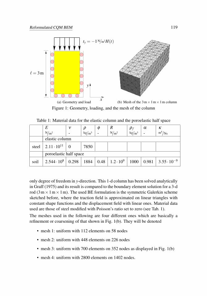
A one dimensional (1-d) column of length 3m as sketched in Fig. 1(a) is considered.It is assumed that the side walls and the bottom are rigid and frictionless. Hence, thedisplacements normal to the surface are blocked and the column is otherwise free toslide only parallel to the wall. At the top, the stress vector ty =−1 N/m2H(t) is given.Due to these restrictions, the 3-d continuum is reduced to a 1-d column with the


` = 3m

x

y

ty =−1 N/m2H(t)

(a) Geometry and load (b) Mesh of the 3m×1m×1m column

Figure 1: Geometry, loading, and the mesh of the column

Table 1: Material data for the elastic column and the poroelastic half space

E ν ρ φ R ρ f α κ

N/m2 - kg/m3 - N/m2 kg/m3 - m4/Ns

elastic column

steel 2.11 ·1011 0 7850

poroelastic half space

soil 2.544 ·108 0.298 1884 0.48 1.2 ·109 1000 0.981 3.55 ·10−9

only degree of freedom in y-direction. This 1-d column has been solved analyticallyin Graff (1975) and its result is compared to the boundary element solution for a 3-drod (3m×1m×1m). The used BE formulation is the symmetric Galerkin schemesketched before, where the traction field is approximated on linear triangles withconstant shape functions and the displacement field with linear ones. Material dataused are those of steel modified with Poisson’s ratio set to zero (see Tab. 1).

The meshes used in the following are four different ones which are basically arefinement or coarsening of that shown in Fig. 1(b). They will be denoted

• mesh 1: uniform with 112 elements on 58 nodes

• mesh 2: uniform with 448 elements on 226 nodes

• mesh 3: uniform with 700 elements on 352 nodes as displayed in Fig. 1(b)

• mesh 4: uniform with 2800 elements on 1402 nodes.


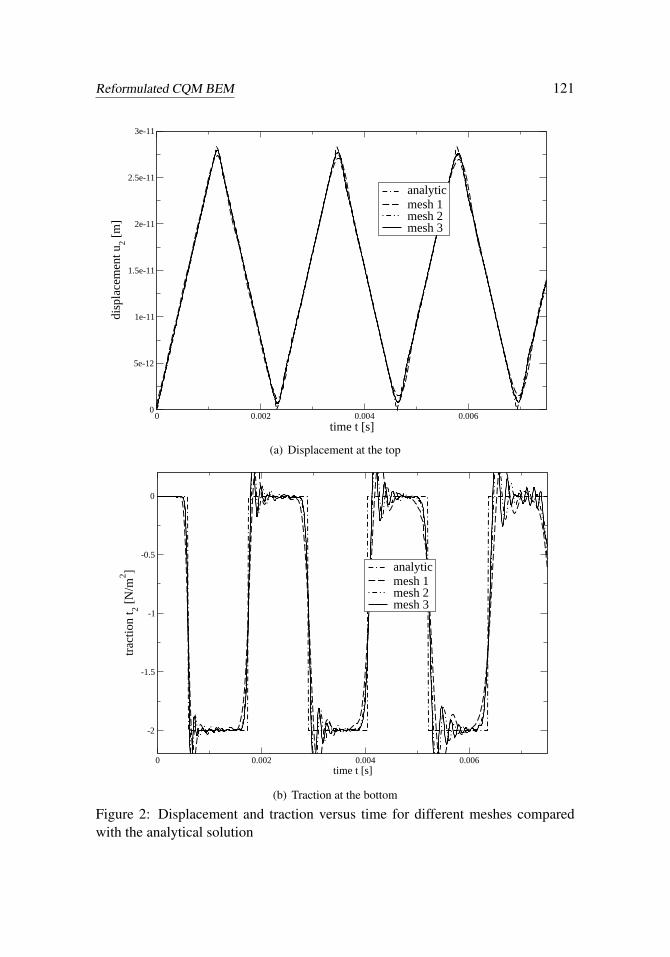
In Fig. 2, the displacement results versus time at the free end are plotted for themeshes 1,2, and 3. The time step size for all three calculations are adjusted toβ = 0.3. This dimensionless value used for the comparison is β = c1∆t/re, with thecharacteristic length of the elements re. Here, the cathethus of the triangles is used.The differences for the displacements in Fig. 2 are not too large. In the secondhalf of the figure, the tractions at the bottom of the column show differences. Thecoarsest mesh 1 yields not satisfactory results for larger times. The overshootingfollowing the jumps in the solution are unavoidable but a refined mesh reducesthe duration of this disturbance. It is exactly the same behavior as in the ’old’CQM based BEM as presented, e.g., in Kielhorn and Schanz (2008). That is whyno comparison between the old formulation and the reformulated version is given.They can not be distinguished in a plot.

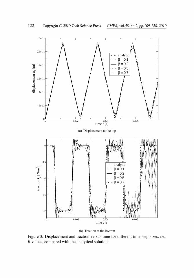
In Fig. 3, the displacement at the top and the traction at the bottom are plottedversus time for different time step sizes. These are expressed with β to have abetter comparison. The results are computed with mesh 2. The instability forthe smallest value β = 0.1 is clearly observed in the traction solution. The otherextreme value, β = 0.7, shows some numerical damping and not the best results forthe traction. All other results are acceptable, where as in the original formulationa value β = 0.2 yields the best results. Hence, also the sensitivity on the choice ofthe time step size is the same as in the original formulation. A time step size in therange 0.1 < β < 0.5 may be recommended.

It must be remarked that here the main advantage of the presented formulationcompared to usual computations in Laplace or Fourier domain can be observed.The parameter responsible for the quality of the results is the time step size andnot any sophisticated parameter of the various numerical inverse transformationalgorithms. This value is oriented on the physics of the problem, i.e., it must beadjusted to the wave speed in relation to the mesh size.

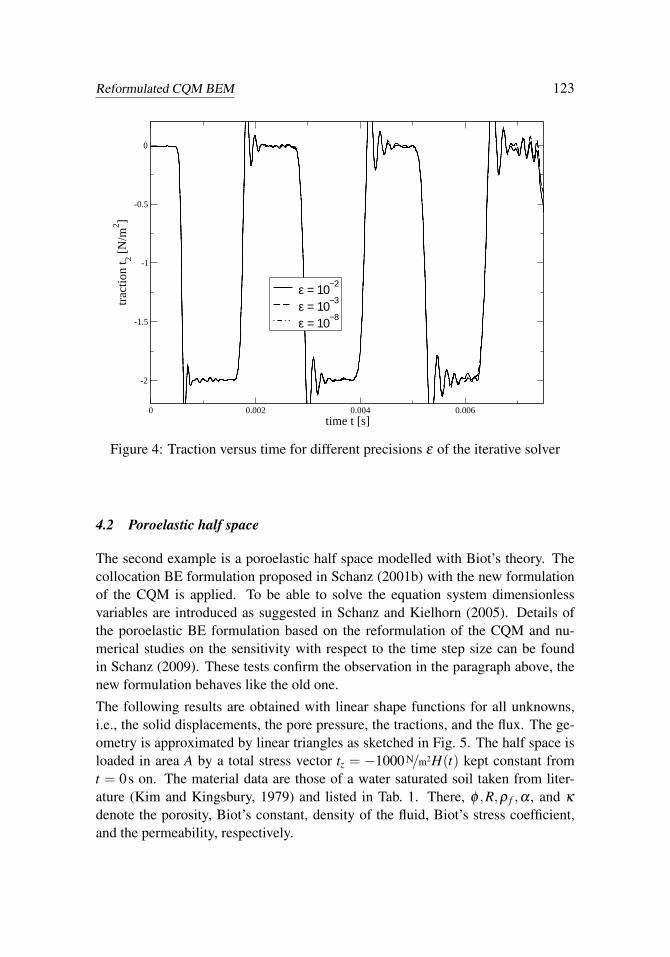
The next parametric study concerns the solution of the equation system. For largerproblems iterative solvers may be used. Hence, the question arise what is the in-fluence of the solver precision on the time dependent results. Here, a GMRESis used. In Fig. 4, the traction solutions for mesh 4 are plotted calculated withdifferent precisions of the GMRES. The displacement solutions are not displayedbecause no differences would be visible. In the traction solution, only for the coarsevalue of ε = 10−2 negative effects for large times may be observed. It may be con-cluded that the solver precision is not so important. But, it must be remarked thatthe solver works in Laplace domain and, hence, eigenfrequencies even if they aredamped may cause problems. Further, it is recommended to think on proper pre-conditioners. Last, it should be mentioned that this ε has nothing to do with the ε

to determine R as discussed at the begining of this section.


0 0.002 0.004 0.006time t [s]

0

5e-12

1e-11

1.5e-11

2e-11

2.5e-11

3e-11

disp

lace

men

t u2 [m

]

analyticmesh 1mesh 2mesh 3

(a) Displacement at the top

0 0.002 0.004 0.006time t [s]

-2

-1.5

-1

-0.5

0

tract

ion

t 2 [N/m

2 ] analyticmesh 1mesh 2mesh 3

(b) Traction at the bottom

Figure 2: Displacement and traction versus time for different meshes comparedwith the analytical solution


0 0.002 0.004 0.006time t [s]

0

5e-12

1e-11

1.5e-11

2e-11

2.5e-11

3e-11

disp

lace

men

t u2 [m

]

analyticβ = 0.1β = 0.2β = 0.5β = 0.7

(a) Displacement at the top

0 0.002 0.004 0.006time t [s]

-2

-1.5

-1

-0.5

0

tract

ion

t 2 [N/m

2 ] analyticβ = 0.1β = 0.2β = 0.5β = 0.7

(b) Traction at the bottom

Figure 3: Displacement and traction versus time for different time step sizes, i.e.,β values, compared with the analytical solution


0 0.002 0.004 0.006time t [s]

-2

-1.5

-1

-0.5

0

tract

ion

t 2 [N/m

2 ]

ε = 10−2

ε = 10−3

ε = 10−8

Figure 4: Traction versus time for different precisions ε of the iterative solver

4.2 Poroelastic half space

The second example is a poroelastic half space modelled with Biot’s theory. Thecollocation BE formulation proposed in Schanz (2001b) with the new formulationof the CQM is applied. To be able to solve the equation system dimensionlessvariables are introduced as suggested in Schanz and Kielhorn (2005). Details ofthe poroelastic BE formulation based on the reformulation of the CQM and nu-merical studies on the sensitivity with respect to the time step size can be foundin Schanz (2009). These tests confirm the observation in the paragraph above, thenew formulation behaves like the old one.

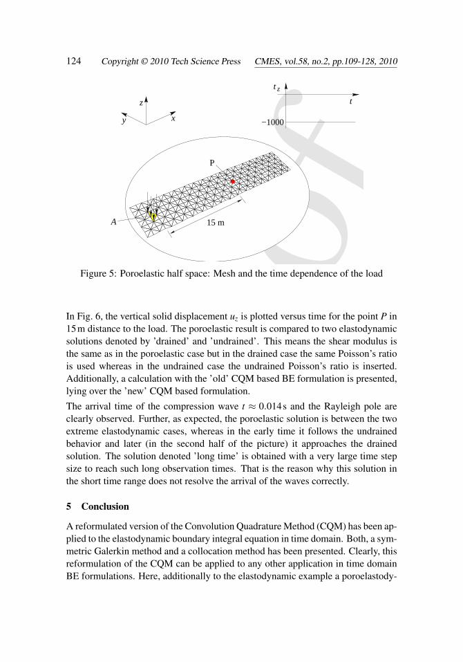
The following results are obtained with linear shape functions for all unknowns,i.e., the solid displacements, the pore pressure, the tractions, and the flux. The ge-ometry is approximated by linear triangles as sketched in Fig. 5. The half space isloaded in area A by a total stress vector tz = −1000 N/m2H(t) kept constant fromt = 0s on. The material data are those of a water saturated soil taken from liter-ature (Kim and Kingsbury, 1979) and listed in Tab. 1. There, φ ,R,ρ f ,α , and κ

denote the porosity, Biot’s constant, density of the fluid, Biot’s stress coefficient,and the permeability, respectively.


CMES Galley Proof Only Please Return in 48 Hours.

Proo

f

16 Copyright © 2009 Tech Science Press CMES, vol.X, no.Y, pp.1-21, 2009

A

z

P

15 m

y

z

x −1000

t

t

Figure 5: Poroelastic half space: Mesh and the time dependence of the load

In Fig. 6, the vertical solid displacement uz is plotted versus time for the point P in244

15m distance to the load. The poroelastic result is compared to two elastodynamic245

solutions denoted by ’drained’ and ’undrained’. This means the shear modulus is246

the same as in the poroelastic case but in the drained case the same Poisson’s ratio247

is used whereas in the undrained case the undrained Poisson’s ratio is inserted.248

Additionally, a calculation with the ’old’ CQM based BE formulation is presented,249

lying over the ’new’ CQM based formulation.250

The arrival time of the compression wave t ≈ 0.014s and the Rayleigh pole are251

clearly observed. Further, as expected, the poroelastic solution is between the two252

extreme elastodynamic cases, whereas in the early time it follows the undrained253

behavior and later (in the second half of the picture) it approaches the drained254

solution. The solution denoted ’long time’ is obtained with a very large time step255

size to reach such long observation times. That is the reason why this solution in256

the short time range does not resolve the arrival of the waves correctly.257

5 Conclusion258

A reformulated version of the Convolution Quadrature Method (CQM) has been ap-259

plied to the elastodynamic boundary integral equation in time domain. Both, a sym-260

metric Galerkin method and a collocation method has been presented. Clearly, this261

Figure 5: Poroelastic half space: Mesh and the time dependence of the load

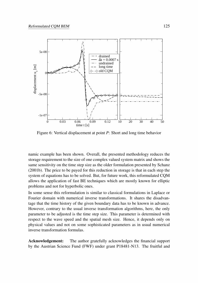
In Fig. 6, the vertical solid displacement uz is plotted versus time for the point P in15m distance to the load. The poroelastic result is compared to two elastodynamicsolutions denoted by ’drained’ and ’undrained’. This means the shear modulus isthe same as in the poroelastic case but in the drained case the same Poisson’s ratiois used whereas in the undrained case the undrained Poisson’s ratio is inserted.Additionally, a calculation with the ’old’ CQM based BE formulation is presented,lying over the ’new’ CQM based formulation.

The arrival time of the compression wave t ≈ 0.014s and the Rayleigh pole areclearly observed. Further, as expected, the poroelastic solution is between the twoextreme elastodynamic cases, whereas in the early time it follows the undrainedbehavior and later (in the second half of the picture) it approaches the drainedsolution. The solution denoted ’long time’ is obtained with a very large time stepsize to reach such long observation times. That is the reason why this solution inthe short time range does not resolve the arrival of the waves correctly.

5 Conclusion

A reformulated version of the Convolution Quadrature Method (CQM) has been ap-plied to the elastodynamic boundary integral equation in time domain. Both, a sym-metric Galerkin method and a collocation method has been presented. Clearly, thisreformulation of the CQM can be applied to any other application in time domainBE formulations. Here, additionally to the elastodynamic example a poroelastody-


0 0.03 0.06 0.09 0.12time t [s]

-1e-07

-5e-08

0

5e-08

disp

lace

men

t uz [m

]

drained∆t = 0.0007 sundrainedlong timeold CQM

10 20 30 40 50

Figure 6: Vertical displacement at point P: Short and long time behavior

namic example has been shown. Overall, the presented methodology reduces thestorage requirement to the size of one complex valued system matrix and shows thesame sensitivity on the time step size as the older formulation presented by Schanz(2001b). The price to be payed for this reduction in storage is that in each step thesystem of equations has to be solved. But, for future work, this reformulated CQMallows the application of fast BE techniques which are mostly known for ellipticproblems and not for hyperbolic ones.

In some sense this reformulation is similar to classical formulations in Laplace orFourier domain with numerical inverse transformations. It shares the disadvan-tage that the time history of the given boundary data has to be known in advance.However, contrary to the usual inverse transformation algorithms, here, the onlyparameter to be adjusted is the time step size. This parameter is determined withrespect to the wave speed and the spatial mesh size. Hence, it depends only onphysical values and not on some sophisticated parameters as in usual numericalinverse transformation formulas.

Acknowledgement: The author gratefully acknowledges the financial supportby the Austrian Science Fund (FWF) under grant P18481-N13. The fruitful and


helpful discussion with L. Banjai and S. Sauter during the author’s stay at the Uni-versity of Zürich is as well gratefully acknowledged.

References

Abreu, A. I.; Carrer, J. A. M.; Mansur, W. J. (2003): Scalar wave propagationin 2D: a BEM formulation based on the operational quadrature method. Eng. Anal.Bound. Elem., vol. 27, pp. 101–105.

Abreu, A. I.; Mansur, W. J.; Carrer, J. A. M. (2006): Initial conditions contri-bution in a BEM formulation based on the convolution quadrature method. Int. J.Numer. Methods. Engrg., vol. 67, pp. 417–434.

Ahmad, S.; Manolis, G. D. (1987): Dynamic analysis of 3-D structures by atransformed boundary element method. Comput. Mech., vol. 2, pp. 185–196.

Antes, H. (1985): A boundary element procedure for transient wave propaga-tions in two-dimensional isotropic elastic media. Finite Elements in Analysis andDesign, vol. 1, pp. 313–322.

Antes, H.; Jäger, M. (1995): On stability and efficiency of 3d acoustic BEprocedures for moving noise sources. In Atluri, S.; Yagawa, G.; Cruse, T.(Eds):Computational Mechanics, Theory and Applications, volume 2, pp. 3056–3061,Heidelberg. Springer-Verlag.

Banjai, L.; Sauter, S. (2009): Rapid solution of the wave equation in unboundeddomains. SIAM J. Numer. Anal., vol. 47, no. 1, pp. 227–249.

Beskos, D. E. (1987): Boundary element methods in dynamic analysis. AMR,vol. 40, no. 1, pp. 1–23.

Beskos, D. E. (1997): Boundary element methods in dynamic analysis: Part II(1986-1996). AMR, vol. 50, no. 3, pp. 149–197.

Cruse, T. A.; Rizzo, F. J. (1968): A direct formulation and numerical solution ofthe general transient elastodynamic problem, I. Aust. J. Math. Anal. Appl., vol. 22,no. 1, pp. 244–259.

Domínguez, J. (1978): Dynamic stiffness of rectangular foundations. Report no.R78-20, Department of Civil Engineering, MIT, Cambridge MA, 1978.

Domínguez, J. (1993): Boundary Elements in Dynamics. Computational Me-chanics Publication, Southampton.

Erichsen, S.; Sauter, S. A. (1998): Efficient automatic quadrature in 3-d GalerkinBEM. Comput. Methods Appl. Mech. Engrg., vol. 157, no. 3–4, pp. 215–224.


García-Sánchez, F.; Zhang, C.; Sáez, A. (2008): 2-d transient dynamic analysisof cracked piezoelectric solids by a time-domain BEM. Comput. Methods Appl.Mech. Engrg., vol. 197, no. 33-40, pp. 3108–3121.

Gaul, L.; Schanz, M. (1999): A comparative study of three boundary elementapproaches to calculate the transient response of viscoelastic solids with unboundeddomains. Comput. Methods Appl. Mech. Engrg., vol. 179, no. 1-2, pp. 111–123.

Graff, K. F. (1975): Wave Motion in Elastic Solids. Oxford University Press.

Guiggiani, M.; Gigante, A. (1990): A general algorithm for multidimensionalcauchy principal value integrals in the boundary element method. J. of Appl. Mech.,vol. 57, pp. 906–915.

Hackbusch, W.; Kress, W.; Sauter, S. A. (2007): Sparse convolution quadraturefor time domain boundary integral formulations of the wave equation by cutoff andpanel-clustering. In Schanz, M.; Steinbach, O.(Eds): Boundary Element Analysis:Mathematical Aspects and Applications, volume 29 of Lecture Notes in Appliedand Computational Mechanics, pp. 113–134. Springer-Verlag, Berlin Heidelberg.

Kausel, E. (2006): Fundamental Solutions in Elastodynamics. CambridgeUniversity Press.

Kielhorn, L.; Schanz, M. (2008): Convolution quadrature method based sym-metric Galerkin boundary element method for 3-d elastodynamics. Int. J. Numer.Methods. Engrg., vol. 76, no. 11, pp. 1724–1746.

Kim, Y. K.; Kingsbury, H. B. (1979): Dynamic characterization of poroelasticmaterials. Exp. Mech., vol. 19, no. 7, pp. 252–258.

Lubich, C. (1988): Convolution quadrature and discretized operational calculus.I. Numer. Math., vol. 52, no. 2, pp. 129–145.

Lubich, C. (1988): Convolution quadrature and discretized operational calculus.II. Numer. Math., vol. 52, no. 4, pp. 413–425.

Lubich, C. (1994): On the multistep time discretization of linear initial-boundaryvalue problems and their boundary integral equations. Numer. Math., vol. 67, pp.365–389.

Lubich, C. (2004): Convolution quadrature revisited. BIT Num. Math., vol. 44,no. 3, pp. 503–514.

Lubich, C.; Schneider, R. (1992): Time discretization of parabolic boundaryintegral equations. Numer. Math., vol. 63, pp. 455–481.

Manolis, G. D. (1983): A comparative study on three boundary element methodapproaches to problems in elastodynamics. Int. J. Numer. Methods. Engrg., vol.19, pp. 73–91.


Mansur, W. J. (1983): A Time-Stepping Technique to Solve Wave Propaga-tion Problems Using the Boundary Element Method. Phd thesis, University ofSouthampton, 1983.

Mansur, W. J.; Carrer, J. A. M.; Siqueira, E. F. N. (1998): Time discontinuouslinear traction approximation in time-domain BEM scalar wave propagation. Int.J. Numer. Methods. Engrg., vol. 42, no. 4, pp. 667–683.

Narayanan, G. V.; Beskos, D. E. (1982): Numerical operational methods fortime-dependent linear problems. Int. J. Numer. Methods. Engrg., vol. 18, pp. 1829–1854.

Nardini, D.; Brebbia, C. A. (1982): A new approach to free vibration analysisusing boundary elements. In Brebbia, C. A.(Ed): Boundary Element Methods, pp.312–326. Springer-Verlag, Berlin.

Partridge, P. W.; Brebbia, C. A.; Wrobel, L. C. (1992): The Dual ReciprocityBoundary Element Method. Computational Mechanics Publication, Southampton.

Peirce, A.; Siebrits, E. (1997): Stability analysis and design of time-steppingschemes for general elastodynamic boundary element models. Int. J. Numer. Meth-ods. Engrg., vol. 40, no. 2, pp. 319–342.

Rizos, D. C.; Karabalis, D. L. (1994): An advanced direct time domain BEMformulation for general 3-D elastodynamic problems. Comput. Mech., vol. 15, pp.249–269.

Schanz, M. (2001): Application of 3-d Boundary Element formulation to wavepropagation in poroelastic solids. Eng. Anal. Bound. Elem., vol. 25, no. 4-5, pp.363–376.

Schanz, M. (2001): Wave Propagation in Viscoelastic and Poroelastic Continua:A Boundary Element Approach, volume 2 of Lecture Notes in Applied Mechanics.Springer-Verlag, Berlin, Heidelberg, New York.

Schanz, M. (2009): Storage reduced poroelastodynamic boundary element for-mulation in time domain. In Ling, H. I.; Smyth, A.; Betti, R.(Eds): PoromechanicsIV, pp. 902–907, Lancaster. DEStech Publications, Inc.

Schanz, M.; Antes, H. (1997): Application of ‘operational quadrature methods’in time domain boundary element methods. Meccanica, vol. 32, no. 3, pp. 179–186.

Schanz, M.; Antes, H. (1997): A new visco- and elastodynamic time domainboundary element formulation. Comput. Mech., vol. 20, no. 5, pp. 452–459.


Schanz, M.; Kielhorn, L. (2005): Dimensionless variables in a poroelastody-namic time domain boundary element formulation. Building Research Journal,vol. 53, no. 2-3, pp. 175–189.

Steinbach, O. (2008): Numerical Approximation Methods for Elliptic BoundaryValue Problems, volume 54 of Texts in Applied Mathematics. Springer.

Wheeler, L. T.; Sternberg, E. (1968): Some theorems in classical elastodynam-ics. Arch. Rational Mech. Anal., vol. 31, pp. 51–90.

Yu, G.; Mansur, W. J.; Carrer, J. A. M.; Gong, L. (1998): Time weighting intime domain BEM. Eng. Anal. Bound. Elem., vol. 22, no. 3, pp. 175–181.

Yu, G.; Mansur, W. J.; Carrer, J. A. M.; Gong, L. (2000): Stability of Galerkinand Collocation time domain boundary element methods as applied to the scalarwave equation. Comput. & Structures, vol. 74, no. 4, pp. 495–506.

Zhang, C. (2000): Transient elastodynamic antiplane crack analysis in anisotropicsolids. Internat. J. Solids Structures, vol. 37, no. 42, pp. 6107–6130.

on a reformulated convolution quadrature based boundary element · pdf fileon a reformulated...

Documents