BOUNDARY ELEMENT METHOD

A case study: the Helmholtz equation.

Li Buyang

Abstract

This is a brief introduction to the boundary element method (BEM) for solving ellipticpartial differential equations (PDEs) when they are reduced to boundary integral equations(BIEs), either using Green’s formulae directly or using other indirect methods. Up to now,the BEM has been well analyzed and become a mature method just like the FEM. In thisnotes, we discuss briefly both the direct and indirect approach of the formulation of bound-ary integral equations. After we have solved the boundary integral equation with BEM,we obtain both the solution and its normal derivative on the boundary, therefore the in-terior values of the solution are given by the boundary integral representation. We sketchthe frame work of Galerkin BEM as well as the collocation BEM in 2D. Some problems ofimplementation of the collocation BEM in 3D was discussed. Most of the content in thisnotes can be found in the lecture notes [7] written in 2006. The matrix generated by BEMis full, which can be solved by using iterative solvers such as GMRES with matrix-vectormultiplication computed with the fast multipole method (FMM). For simplicity, we focuson the discussion of Helmholtz equation. Other elliptic equations can be analyzed similarlyprovided the fundamental solution is available.

Key words: Helmholtz equation, fundamental solution, Green’s formula, boundary integralrepresentation, boundary integral equation, boundary element method, multipole expansion.

1 Introduction

The boundary element method (BEM) is a numerical computational method of solving lin-ear elliptic PDEs which have been formulated as equivalent boundary integral equations. Itcan be applied in many areas of engineering and science including fluid mechanics, acoustics,electromagnetics, and fracture mechanics. The boundary element method attempts to use thegiven boundary conditions to fit boundary values into the integral equation, rather than val-ues throughout the space defined by a partial differential equation. Once this is done, in thepost-processing stage, the integral equation can then be used again to calculate numericallythe solution directly at any desired point in the interior of the solution domain. The BEM isoften more efficient than other methods, including finite elements method, if the solution is onlydesired at some particular point of the domain. Moreover, the BEM is especially efficient tosolve exterior problems, which reduce the infinite domain problem to a finite domain problem oflower dimension. However, for many problems boundary element methods are significantly lessefficient than volume-discretisation methods (finite element method, finite difference method,finite volume method). Boundary element formulations typically give rise to fully populatedmatrices. Compression techniques such as multipole expansions can be used to ameliorate theseproblems, though at the cost of added complexity and with a success-rate that depends heavilyon the nature of the problem being solved and the geometry involved. The linear system can

1

be solved by using the iterative solver GMRES with matrix-vector product computed with themultipole expansion method. Then the cost of a matrix-vector product can be reduced to O(N),where N is the size of the linear system.

The BEM is only applicable to problems for which Green’s functions is available and isonly efficient to problems that no nonlinearities appear in the domain, though in principle,nonlinearities can be included in the formulation by introducing volume integrals which thenrequire the volume to be discretised before solution can be attempted, removing one of themost often cited advantages of BEM. These usually involve fields in linear homogeneous media.This places considerable restrictions on the range and generality of problems to which boundaryelements can usefully be applied.

The Green’s functions, or fundamental solutions, are often problematic to integrate as theycontains singularity at the source point. Integrating such singular fields is not easy. For simpleelement geometries, analytical integration can be used. For more general elements, it is possibleto design purely numerical schemes that adapt to the singularity, but at great computationalcost.

In the next section, we give a direct formulation of boundary integral representation of thesolution for the Helmholtz equation as well as the conventional and hypersingular boundaryintegral equations.

2 Direct formulation of BIEs

The direct boundary integral formulation uses Green’s formula to reduce the differential equationin the domain to a boundary integral equation. For instance, we consider the electromagneticscattering problem outside a bounded Lipschitz domain Ω in Rn, which can be described as anexterior boundary value problem:

∆u + k2u = 0, in Rn\Ω,

∂nu = g, on ∂Ω,(2.1)

with the Sommerfeld radiation condition

limr→∞

√r

(∂u

∂r− iku

)= 0, r = |x| (2.2)

uniformly in all directions. The Sommerfeld radiation condition is to ensure that the solutiondecreases fast enough as |x| → ∞. For details of the existence and uniqueness analysis forthis boundary value problem we refer to [1, 5]. Here and follows, we assume that the problem(2.1)-(2.2) has a unique solution.

It is not difficult to verify that the Helmholtz equation in Rn has a fundamental solution

G(x, y) =

i

4H

(1)0 (k|x− y|), for n = 2,

eik|x−y|

4π|x− y| , for n = 3,

which satisfies−(∆x + k2)G(x, y) = δ(x− y)

2

in the sense of distributions for any fixed y ∈ Rn. If u ∈ C2(R2\Ω) ∩ H1loc(Rn\Ω) satisfies

Helmholtz equation in the exterior domain Rn\Ω and the Sommerfeld radiation condition uni-formly as |x| → ∞, then by using Green’s formulae formally, i.e.

− k2

∫

Rn\Ωuv dx +

∫

Rn\Ω∇u · ∇v dx =

∫

Rn\Ωu(−∆v − k2v) dx−

∫

∂Ωu ∂nv dσ, (2.3)

− k2

∫

Rn\Ωuv dx +

∫

Rn\Ω∇u · ∇v dx =

∫

Rn\Ωv(−∆u− k2u) dx−

∫

∂Ωv∂nu dσ, (2.4)

with v(x) = G(x, y), where n is the unit inner normal vector on the boundary ∂Ω, we obtainthe boundary integral representation

u(y) =∫

∂Ω

(∂G(x, y)∂n(x)

u(x)−G(x, y) ∂nu(x))

dσ(x), y ∈ Ω, (2.5)

By differentiating the equation (2.5), we derive the boundary integral representation of thepotential gradients

∂u(y)∂yi

=∫

∂Ω

(∂2G(x, y)∂yi∂n(x)

u(x)− ∂G(x, y)∂yi

∂nu(x))

dσ(x), y ∈ Ω. (2.6)

Taking trace and normal derivative of the equation (2.5), we obtain the conventional boundaryintegral equation (CBIE)

12u(y) =

∫

∂Ω

(∂G(x, y)∂n(x)

u(x)−G(x, y) ∂nu(x))

dσ(x), y ∈ ∂Ω (2.7)

and the hypersingular boundary integral equation (HBIE)

12∂nu(y) =

∫

∂Ω

∂2G(x, y)∂n(x)∂n(y)

u(x)dσ(x)−∫

∂Ω

∂G(x, y)∂n(y)

∂nu(x)dσ(x), y ∈ ∂Ω, (2.8)

The above equations are valid everywhere except at the corner of the boundary ∂Ω. For weaksolutions u ∈ H1(Ω), the CBIE is valid in H1/2(∂Ω) and the HBIE is valid in H−1/2(∂Ω).

We see that the solution of the exterior Neumann problem satisfies the hypersingular bound-ary integral equation

Hu = −(12I + T ∗)g, (2.9)

where H is the hypersingular operator

Hu(y) = −∫

∂Ω

∂2G(x, y)∂n(x)∂n(y)

u(x)dσ(x), y ∈ ∂Ω

and T ∗ is defined by

T ∗g(y) =∫

∂Ω

∂G(x, y)∂n(y)

g(x)dσ(x), y ∈ ∂Ω.

The integral equation (2.9) has a unique solution if and only if the original exterior problemhas a unique solution. In that case,

u = −H−1(12I + T ∗)g.

3

The operator on the right hand side relates the boundary value of the solution to the its normalderivative and hence called the Dirichlet-to-Neumann map. However, the DtN mapping is notknown analytically for domains with general geometry. The integral equation (2.9) has to besolved numerically.

After the boundary integral equation (2.9) is solved, the values of the solution and its gra-dients in the domain Rn\Ω are given by the boundary integral representations (2.5) and (2.6).Therefore, the n-dimensional problem in the exterior domain Rn\Ω is converted to a (n − 1)-dimensional problem on the boundary ∂Ω.

3 An indirect formulation

We see that the integral equation obtained by the direct formulation is somehow complicated.In another way, we try to look for a simple solution which can be expressed as

u(y) = −∫

∂Ω

∂G(x, y)∂n(x)

ψ(x)dσ(x), y ∈ Ω. (3.10)

By the property of the fundamental solution, for any function ψ ∈ H1/2(∂Ω), the function udefined above satisfies Helmholtz equation in the domain Rn\Ω and the Sommerfeld radiationcondition at infinity. The only restriction we have to impose on ψ is that the solution u satisfiesthe Neumann boundary condition, i.e.

−∫

∂Ω

∂2G(x, y)∂n(y)∂n(x)

ψ(x)dσ(x) = g(y), y ∈ ∂Ω. (3.11)

By noting that the hypersingular operator is of Fredholm type with zero index [5], it is easy toobserve that the existence and uniqueness of solution of the above integral equation is equivalentto that of the exterior problem (2.1)-(2.2). Therefore, we can solve the HBIE

Hψ = g (3.12)

with an unknown density ψ which does not has an explicit physical meaning. Then the solutionvalues in the exterior domain is given by (3.10).

4 Galerkin BEM

The Galerkin method is similar for both 2D and 3D problems. For simplicity, we illustrate theidea in the 2D framework. We denote 〈φ, ψ〉 =

∫∂Ω φψdσ for any φ, ψ defined on the boundary

∂Ω such that the integral has a meaning. The variational formulation of the integral equation(3.12) consists of finding u ∈ H1/2(∂Ω) such that

〈Hψ, v〉 = 〈g, v〉, ∀ v ∈ H1/2(∂Ω). (4.13)

Using the strong ellipticity of the hypersingular operator [5], i.e.

〈Hψ,ψ〉 ≥ c‖ψ‖2H1/2(∂Ω)

− C‖ψ‖2L2(∂Ω), ∀ψ ∈ H1/2(∂Ω)

and the invertibility of the mapping

H : H1(∂Ω) → L2(∂Ω),

4

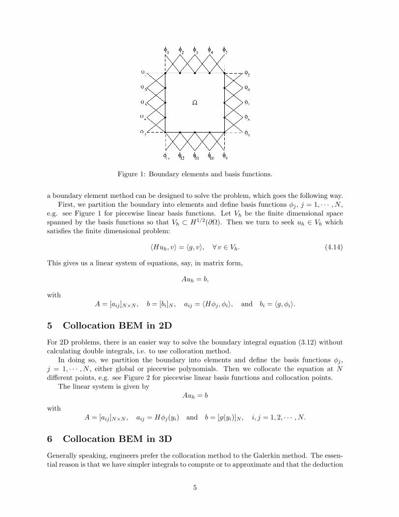
Figure 1: Boundary elements and basis functions.

a boundary element method can be designed to solve the problem, which goes the following way.First, we partition the boundary into elements and define basis functions φj , j = 1, · · · , N ,

e.g. see Figure 1 for piecewise linear basis functions. Let Vh be the finite dimensional spacespanned by the basis functions so that Vh ⊂ H1/2(∂Ω). Then we turn to seek uh ∈ Vh whichsatisfies the finite dimensional problem:

〈Huh, v〉 = 〈g, v〉, ∀ v ∈ Vh. (4.14)

This gives us a linear system of equations, say, in matrix form,

Auh = b,

withA = [aij ]N×N , b = [bi]N , aij = 〈Hφj , φi〉, and bi = 〈g, φi〉.

5 Collocation BEM in 2D

For 2D problems, there is an easier way to solve the boundary integral equation (3.12) withoutcalculating double integrals, i.e. to use collocation method.

In doing so, we partition the boundary into elements and define the basis functions φj ,j = 1, · · · , N , either global or piecewise polynomials. Then we collocate the equation at Ndifferent points, e.g. see Figure 2 for piecewise linear basis functions and collocation points.

The linear system is given byAuh = b

withA = [aij ]N×N , aij = Hφj(yi) and b = [g(yi)]N , i, j = 1, 2, · · · , N.

6 Collocation BEM in 3D

Generally speaking, engineers prefer the collocation method to the Galerkin method. The essen-tial reason is that we have simpler integrals to compute or to approximate and that the deduction

5

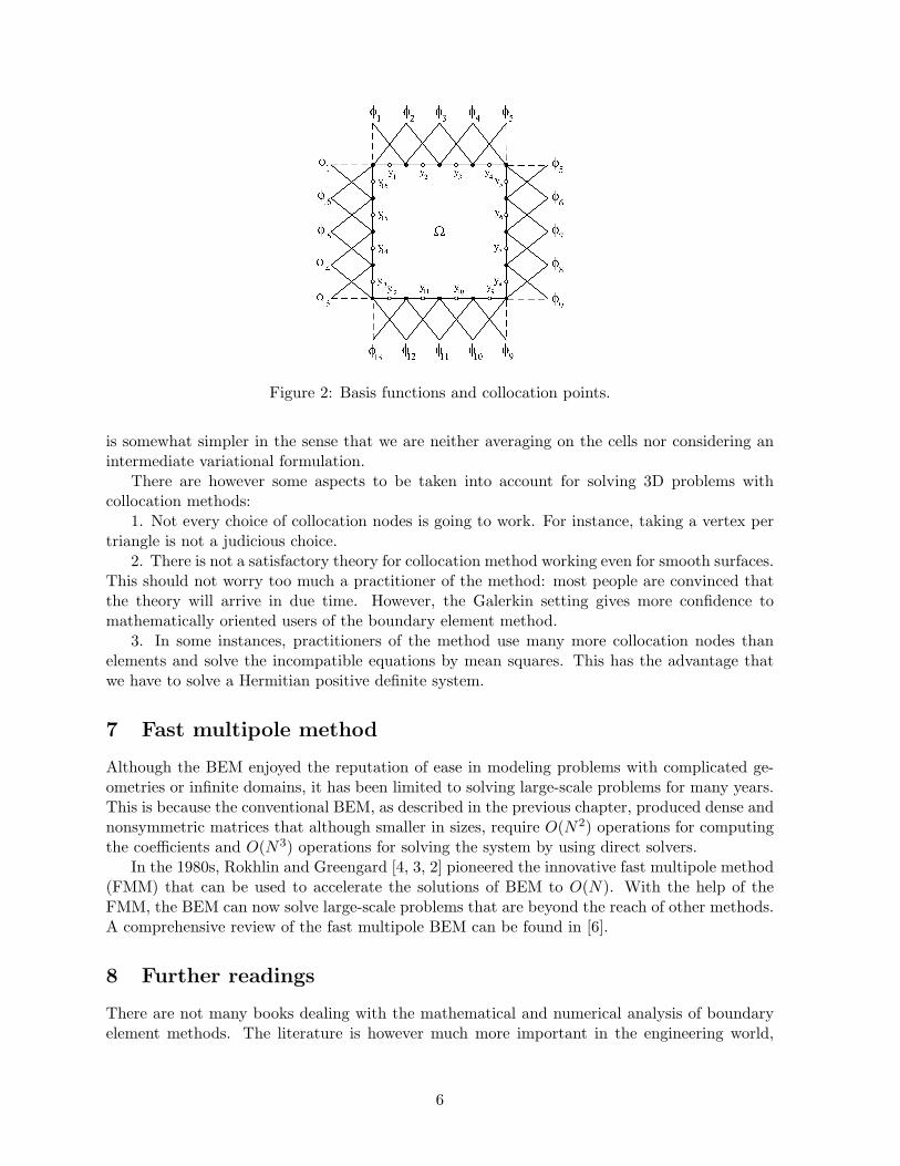
Figure 2: Basis functions and collocation points.

is somewhat simpler in the sense that we are neither averaging on the cells nor considering anintermediate variational formulation.

There are however some aspects to be taken into account for solving 3D problems withcollocation methods:

1. Not every choice of collocation nodes is going to work. For instance, taking a vertex pertriangle is not a judicious choice.

2. There is not a satisfactory theory for collocation method working even for smooth surfaces.This should not worry too much a practitioner of the method: most people are convinced thatthe theory will arrive in due time. However, the Galerkin setting gives more confidence tomathematically oriented users of the boundary element method.

3. In some instances, practitioners of the method use many more collocation nodes thanelements and solve the incompatible equations by mean squares. This has the advantage thatwe have to solve a Hermitian positive definite system.

7 Fast multipole method

Although the BEM enjoyed the reputation of ease in modeling problems with complicated ge-ometries or infinite domains, it has been limited to solving large-scale problems for many years.This is because the conventional BEM, as described in the previous chapter, produced dense andnonsymmetric matrices that although smaller in sizes, require O(N2) operations for computingthe coefficients and O(N3) operations for solving the system by using direct solvers.

In the 1980s, Rokhlin and Greengard [4, 3, 2] pioneered the innovative fast multipole method(FMM) that can be used to accelerate the solutions of BEM to O(N). With the help of theFMM, the BEM can now solve large-scale problems that are beyond the reach of other methods.A comprehensive review of the fast multipole BEM can be found in [6].

8 Further readings

There are not many books dealing with the mathematical and numerical analysis of boundaryelement methods. The literature is however much more important in the engineering world,

6

where you will be able to find many details on algorithms, implementation and especially differentproblems where boundary element techniques apply.

The book

Boundary Element Methods, by Goong Chen, Jingmin Zhou, Academic Press, 1992.

details the boundary integral formulations for the Laplace, Helmholtz, Navier-Lame (linearelasticity) and biharmonic (Kirchhoff plate) equations. The Sobolev theory is explained with carein the case of smooth interfaces. The fundamentals of Sobolev theory and finite element methodare carefully explained. There are also some explanations on pseudodifferential operators, atheory that allows for a generalization of the behavior of all the boundary integral operators forsmooth boundaries. The section on numerical analysis is not very long and right now it is notup-to-date.

The whole theory on boundary integral formulations based on the theory of elliptic operatorsis explained with an immense care and taste for mathematical detail in

Strongly Elliptic Systems and Boundary Integral Equations, by William McLean,Cambridge University Press, 2000.

This is a book of hard mathematics, where you will learn a lot but are asked to have patience.It does not cover numerical analysis.

Following is a book with discussions of how to implement FMM in solving the various bound-ary integral equations.

Fast Multipole Boundary Element Method, by Yijun Liu, Cambridge university press, 2009.

References

[1] D. Colton and R. Kress, Integral equation methods in scattering theory, Wiley-Interscience, New York,1983.

[2] L.F. Greengard, The rapid evaluation of potential fields in particle systems, MIT Press, Cambridge,MA, 1988.

[3] L.F. Greengard, V. Rokhlin, A fast algorithm for particle simulations, J. Comput. Phyys. 73, 325-348,1987.

[4] V. Rokhlin, Rapid solution of integral equations of classical potential theory, J. Comput. Phyys. 60,187-207, 1985.

[5] William McLean, Strongly elliptic systems and boundary integral equations, Cambridge universitypress, 2000.

[6] N. Nishimura, Fast multipole accelerated boundary integral equation methods, Appl. Mech. Rev. 55,299-324, 2002.

[7] F.J. Sayas, Introduction to the boundary element method. A case study: the Helmholtz equation,Lecture notes, 2006.

7