the boundary element
DESCRIPTION
Boundary Element methodTRANSCRIPT

7/17/2019 The Boundary Element
http://slidepdf.com/reader/full/the-boundary-element 1/201
Cover

7/17/2019 The Boundary Element
http://slidepdf.com/reader/full/the-boundary-element 2/201
Page i
The Boundary Element Method

7/17/2019 The Boundary Element
http://slidepdf.com/reader/full/the-boundary-element 3/201
Page ii
To our wives:
Shayla Ali and Lalitha Rajakumar
and our children:
Aleef & Teeasha Ali, and Vinod & Anita Rajakumar

7/17/2019 The Boundary Element
http://slidepdf.com/reader/full/the-boundary-element 4/201
Page iii
The Boundary Element Method
Applications in Sound and Vibration
Ashraf Ali
Engineering Solution and Support (ESAS), Bellevue, Washington (Formerly with Ansys, Inc., Canonsburg, Pennsylvania)
Charles Rajakumar
Ansys, Inc., Canonsburg, Pennsylvania
A.A.BALKEMA PUBLISHERS
LISSE/ABINGDON/EXTON (PA)/TOKYO

7/17/2019 The Boundary Element
http://slidepdf.com/reader/full/the-boundary-element 5/201
Page iv
Library of Congress Cataloging-i n-Publication Data A Catalogue record for this book is available from the Library of Congress
Cover design: Miranda Bourgonjen
Copyright © 2004 Taylor & Francis Group plc, London, UK
All rights reserved. No part of this publication or the information contained herein may be reproduced, stored in a retrieval system, or transmitted in any form or by any means, electronic, mechanical, by photocopying, recording or otherwise, without written prior
permission from the publishers.
Although all care is taken to ensure the integrit y and quality of this publicati on and the information herein, no responsibility is assumed by the publishers nor the author
for any damage to property or persons as a result of operation or use of this publicati on and/or the information contained herein.
Published by: A.A.Balkema Publishers (Leiden, The Netherlands),a member of Taylor & Francis Group plc.
http://balkema.tandf.co.uk and www.tandf.co.ukThis edition published in the Taylor & Francis e-Library, 2005.
To purchase your own copy of this or any of Taylor & Francis or Routledge’s collection of thousands of eBooks please go to www.eBookstore.tandf.co.uk.
ISBN 0-203-02446-X Master e-book ISBN
ISBN 90 5809 657 2 (Print Edition)

7/17/2019 The Boundary Element
http://slidepdf.com/reader/full/the-boundary-element 6/201
Page v
Contents
Preface vii
Acknowledgements ix
Abbreviations xi
1 Introduction 1
1.1 Why the boundary element method? 1
1.2 Typical applications of the boundary element method 2
1.3 Emergence of the boundary element method 3
1.4 History of boundary element eigenformulations 6
1.5 Organization of the book 9
2 Boundary Element Method Fundamentals 11
2.1 Introduction 11
2.2 Direct method: weighted residuals 12
2.3 Examples 19
2.4 Direct method: Green’s integral theorem 21
2.5 Indirect method 23
2.6 Body forces 26
3 Isoparametric Boundary Elements 31
3.1 Introduction 31
3.2 Two- dimensional linear boundary elements 31
3.3 Higher-order elements in 2-D 34
3.4 Boundary elements in 3-D 36
3.5 Examples 42
4 Anisotropy, Axisymmetry and Zoning 49
4.1 Introduction 49
4.2 Anisotropic materials 49
4.3 Axisymmetric problems 51
4.4 Inhomogeneous regions and zoning 54
5 Time-Harmonic Analysis in Acoustics and Elasticity 57
5.1 Introduction 57
5.2 Acoustics 57
5.3 Elasticity 62
6 Dynamic Analysis: Acoustics and Elasticity 65
6.1 Introduction 65
6.2 Eigenvalue problem in acoustics 71
6.3 Eigenvalue problem in elasticity 72
6.4 Characteristic equation for eigenvalues 72

7/17/2019 The Boundary Element
http://slidepdf.com/reader/full/the-boundary-element 7/201
Page vi
7 Basics of Algebraic Eigenvalue Problem Formulation 77
7.1 Introduction 77
7.2 Development of BE algebraic eigenvalue problem 77
7.3 Formulation of Internal Cell Method 78
7.4 Example of internal cell method: rectangular plate vibration 80
8 Algebraic Eigenvalue Problem in Boundary Elements 87
8.1 Introduction 87 8.2 Eigenproblem using dual reciprocity method in acoustics 87
8.3 Eigenproblem using particular integral method in elasticity 96
9 Advanced Concepts in Boundary Element Algebraic Eigenproblem 107
9.1 Introduction 107
9.2 Algebraic eigenvalue formulation using fictitious function method 108
9.3 Example problems using fictitious function method 111
9.4 Effect of internal collocation points on eigensolutions 112
9.5 Polynomial-based particular integral method 116
9.6 Multiple reciprocity method (MRM) 121
9.7 Series expansion methods (SEM) with matrix augmentation 127
10 Acoustic Fluid-Structure Interaction Problems 129
10.1 Introduction 129
10.2 Boundary element-finite element coupled eigenanalysis of fluid-structure system 130
10.3 Acoustic eigenproblem for enclosures with dissipative boundaries 137
10.4 Examples of acoustic eigenproblem with sound absorption 141
11 Solution Methods of Eigenvalue Problems 149
11.1 Introduction 149
11.2 Lanczos-based subspace approach 149
11.3 Lanczos recursion method 150
11.4 Example problems 157
11.5 Summary statements on the non- symmetric Lanczos eigensolver 160
11.6 Damped system eigenvalue problem solution 161
11.7 Lanczos two- sided recursion for the quadratic eigenvalue problem 162
11.8 Summary statements on eigenvalue computation algorithms 170
12 Discussion and Future Research 171
12.1 Discussion on boundary element eigenvalue methodologies 171
12.2 Comparison of eigenanalysis using BEM and FEM 172
12.3 Topics not covered in the book 173
12.4 Future research on BEM eigenanalysis 174
References 177
Index 187

7/17/2019 The Boundary Element
http://slidepdf.com/reader/full/the-boundary-element 8/201
Page vii
Preface
The boundary element method is a powerful discretization tool in computational mechanics. However, the eigenvalue analysis procedures within the boundary element
discretization process are still in a developing stage. To our knowledge, this is the first-ever book dedicated entirely to the subject of boundary element eigenvalue
formulations. All the techniques of boundary element eigenvalue analysis currently available in the literature are reviewed and presented in the book. For each technique,
a detailed theoretical formulation is presented, followed by numerical illustrations. The advantages and disadvantages of each method in terms of computational
efficiencies, generalities, and formulation difficulties are also presented.The book includes detailed formulations on linear and quadratic eigensolvers for unsymmetric matrices since boundary element matrices are naturally unsymmetric.
The book also sheds light on the ongoing debate on the choice of technique, the relative merits of eigenanalyses based on the boundary element and finite element
methods, the unresolved issues that require immediate attention and the future direction of research in this area.
The mode-frequency analyses of vibrating structures and the computation of resonant frequencies of acoustical cavities are now routinely performed in the industry.
The eigenanalysis based on the boundary element method holds promise of becoming a user-friendly and popular procedure with practicing engineers simply because
here it can avoid the tedious and time-consuming process of creating an adequate mesh for their models. Some applications include:
Elasticity Area:
1. Machines (automobiles, aircraft, etc.);
2. Machine parts such as connectors, shafts, gears, fasteners such as screws, pins, etc;
3. Other equipment that is subjected to vibrations during normal operation;
4. Structures (bridges, buildings, etc.).
Acoustics Area:
1. Acoustic enclosures such as auditoriums, theaters, passenger-car and train cabins, etc.;2. Hi-Fi sound equipment such as loudspeakers;
3. Fluid-filled structures such as oil tankers;
4. Noise control of structures such as automobile mufflers; aircraft fuselages, rooms housing vibrating machines, etc.
Furthermore, eigenvalue analysis forms the basis for subsequent mode-based dynamic analyses, such as mode superposition transient analysis, spectrum analysis, and
random vibration analysis.

7/17/2019 The Boundary Element
http://slidepdf.com/reader/full/the-boundary-element 9/201
Page viii
Before the advent of practical numerical methods like the finite element method, engineers conducted experiments on prototypes for determining natural frequencies.
Starting in the 1970s, computer programs based on the finite element method were available. Although the finite element method is a versatile computational technique,
it requires a much longer data-preparation time than the boundary element method. Specifically, engineers are forced to spend a significant amount of time in generating
an adequate mesh for the model problem. Despite the introduction of a few automatic mesh-generation algorithms in the commercial finite element programs, engineers
still continue to struggle in creating meshes of acceptable quality.
The boundary element method, on the other hand, is a boundary technique where only the boundary of the domain is required to be meshed, thereby simplifying data
preparation efforts significantly. Among other benefits, the overall physical time spent by engineers to perform the analysis is reduced significantly, and the analysis
process becomes more user-friendly.
The book presents the eigenvalue analysis techniques that use the boundary element method. The boundary element method does not easily lend itself to eigenvalue
formulations, especially algebraic eigenvalue formulations. Consequently, publications on boundary element algebraic eigenvalue formulations did not come out until themid-1980s, although the boundary element method has been around since the late 1960s. However, non-algebraic boundary element eigenvalue analysis, which is not a
practical analysis technique, appeared in the literature of the mid-1970s. For historical reasons, the book presents some materials related to the non-algebraic boundary
element eigenvalue analysis techniques.
Three general purpose boundary element computer programs (GPBEST, BEASY, and SYSNOISE) offer boundary element eigenvalue analysis capabilities. This
book will hopefully satisfy the needs of engineers to acquire a detailed knowledge on the subject. The capabilities of the commercial programs, such as those
mentioned, may be enhanced through the implementation of some of the different methods of performing boundary element eigenvalue analysis presented in the book.
This book should also encourage the development of new and more powerful computer programs on boundary element eigenvalue analysis.
The book can be used in the graduate classes on “computational mechanics” and “boundary element methods”. The researchers in universities and industries,
practicing engineers, mathematicians, computer scientists, physicists, chemists and chemical engineers, and researchers in bio-medical fields can also use it as a
reference.
Ashraf Ali
Seattle, Washington
Charles Rajakumar
Pittsburgh, Pennsylvania

7/17/2019 The Boundary Element
http://slidepdf.com/reader/full/the-boundary-element 10/201
Page ix
Acknowledgements
We are indebted to Ansys, Inc., Canonsburg, Pennsylvania for getting us interested in the subject of boundary element method. We are also grateful to Sidney
Solomon of The Solomon Press of New York in giving us encouragement and valuable suggestions in the preparation and completion of the book.

7/17/2019 The Boundary Element
http://slidepdf.com/reader/full/the-boundary-element 11/201
Page x
This page intentionally left blank.

7/17/2019 The Boundary Element
http://slidepdf.com/reader/full/the-boundary-element 12/201
Page xi
Abbreviations
1-D One-dimensional, One dimension
2-D Two-dimensional, Two dimensions
3-D Three-dimensional, Three dimensions
BE Boundary Element
BEM Boundary Element Method
BIEM Boundary Integral Equation Method
CPU Central Processing Unit
DRM Dual Reciprocity Method
DSM Determinant Search Method
FE Finite Element
FEM Finite Element Method
FFM Fictitious Function Method
GSF Global Shape Function
ICM Internal Cell Method
MRM Multiple Reciprocity Method
NACA National Advisory Committee for Aeronautics
PIM Particular Integral Method
PSF Polynomial Shape Function
SEM Series Expansion Method

7/17/2019 The Boundary Element
http://slidepdf.com/reader/full/the-boundary-element 13/201
Page xii
This page intentionally left blank.
7/17/2019 The Boundary Element
http://slidepdf.com/reader/full/the-boundary-element 14/201
Page 1
Chapter 1
Introduction
1.1. Why the boundary element method?
In the last thirty to thirty-five years the Boundary Element Method (BEM) has emerged as one of the most powerful computational tools for solving a wide variety of problems in science and engineering. While the Finite Element Method (FEM) is known to be versatile, the BEM brings with it the extraordinary feature of being simple
in geometric data preparation. This particular feature of BEM derives from the fact that the discretization of the problem domain is confined to the boundary alone, i.e.,
the unknowns to be solved for are only on the boundary. The solution inside the domain can be computed as a post-processing step after the unknowns on the
boundary points have been solved for.
In the FEM, the entire domain must be discretized in order to set up the algebraic equations and get solutions. It not only increases the number of equations that must
be solved, but also burdens the user with generating an adequate mesh on the surface as well as in the interior of the domain. Despite the advent of a number of
algorithms of automatic mesh generation to be used with the FEM, the users of the FEM today are still forced to allocate more than half of their time in creating suitable
meshes for their problems.
Since the BEM reduces the problem dimension by one, two-dimensional (2-D) problems can be solved in one dimension and three-dimensional (3-D) problems can
be posed in two dimensions. Therefore, only a line mesh around the boundary of the domain is needed in two dimensions and a surface mesh for 3-D geometries. It
leads to dramatic reductions in mesh generation efforts, resulting in significant savings in processing time put in by an engineer toward solving the problem at hand. This
particular property of the BEM makes it an attractive numerical analysis tool.
The BEM is an integral-type of numerical analysis procedure in which the integration of the governing differential equations is performed before the numerical analysis
has been carried out. The FEM, on the other hand, is a differential-type numerical analysis technique because the numerical analysis part is performed first followed by
the integration of the governing differential equation. The FEM may also be designated as a local technique. Here the entire problem domain is divided into “finiteelements,” which form the building blocks for reconstructing the whole domain. The numerical analysis is performed on the individual elements. The finite elements are
then assembled for the entire domain, which is equivalent to the integration of the governing differential equation. The compatibility between adjacent elements is
ensured during the process

7/17/2019 The Boundary Element
http://slidepdf.com/reader/full/the-boundary-element 15/201
Page 2
of assembly of the element matrices, and the equilibrium of the individual element ensures the overall equilibrium of the whole domain after assembly.
The BEM is a global numerical analysis procedure. The solution of the problem is found by superposing singular solutions distributed over the entire boundary of the
problem. The singular source located at one point of the boundary exerts influence on each and every point on the boundary of the problem. When this influence of a
single source for a discretized boundary is summed over all the boundary segments/elements, it fills the entire row of the final algebraic matrix equation. Therefore, a
separate assembly procedure is not called for. The equilibrium is globally satisfied at once for the whole domain.
The BEM is more efficient than the FEM for several classes of problems, viz., infinite-domain problems such as those in acoustics, electrostatics, and
electromagnetics, and problems with stiff gradients such as those in fracture mechanics. In some cases, a combined BEM-FEM procedure, in which the strengths of
both methods can be exploited, is found to be optimal. The FEM is known to handle inhomogeneities and nonlinearities in the domain more efficiently. Therefore, the
part of the domain that contains inhomogeneities and/or nonlinearities can be modeled using the finite elements, whereas the part that is homogeneous and/or extends to
infinity may be modeled using boundary elements.
1.2. Typical applications of the boundary element method
Consider the return-and-go conductor problem, also known as the magnetic dipole problem, in which two conductors in free space carry current in opposite directions
to infinity. The problem is to compute the magnetic flux density distribution both inside and outside of the conductors. Figure 1.1 shows four different ways of solving it.
In the first method, the problem is solved using the BEM alone. Only the boundaries of the conductors are required to be discretized in order to model both the
interiors of the conductors and the infinite-extent external domain. In the second method, the interior of one of the conductors is meshed using finite elements, whereas
the interior of the other conductor as well as the infinite-extent exterior domain are modeled with the help of boundary elements. In the third method, the interiors of
both conductors are modeled using finite elements, while the infinite-extent external domain is modeled using boundary elements. In the fourth method, the problem is
solved using finite elements for both conductors and a portion of the external domain and boundary elements beyond.
In the first three cases, the zero-potential and zero-flux boundary conditions at infinity are implicitly satisfied by the boundary elements, although the discretization is
confined to the surface of the conductors. Since the BEM is a global technique, the conductors that are physically disconnected at the two-dimensional (2-D) plane are
easily modeled without requiring the domain between the conductors to be discretized. Also, in the first case, both the interior and the exterior domains are modeled
using just one discretization at the conductor boundaries. In other words, in the BEMs, the boundary discretization used to model the interior domain can be used tomodel the external domain just by flipping the outward normal. Note that because of symmetry and anti-symmetry, the return-and-go conductor problem is, in practice,
solved using only a quarter of the domain.

7/17/2019 The Boundary Element
http://slidepdf.com/reader/full/the-boundary-element 16/201
Page 3
Figure 1.1. The return-and-go conductor problem. (a) Both conductors and exterior domain are modeled using BE alone; (b) interior ofone conductor and exterior domain are modeled using BE while the interior of the other conductor is modeled using FE; (c)interiors of both conductors are modeled using FE, while the exterior domain is modeled using BE; (d) interiors of bothconductors and a portion of the exterior domain are modeled using FE while the exterior domain is modeled using BE.
Over the years, BEMs have been applied to many branches of engineering science, such as: heat conduction, elastostatics, elastodynamics, elastoplasticity,viscoplasticity, acoustics, fracture mechanics, fluid flow, fluid-structure interaction problems, and electromagnetics.
However, the eigenvalue analysis formulations in the context of BEMs did not appear before the late 1970s. This is because the BEM does not easily lend itself to an
algebraic eigenvalue formulation. The evolutionary history of different types of eigenvalue formulations with the BEMs will be presented later in this chapter. Before that,
a brief chronological history of the emergence of the BEM itself is presented below.
1.3. Emergence of the boundary element method
As mentioned earlier, the BEM is an integral equation technique. The study of the integral equations started many decades before the boundary integral equation
method (BIEM) emerged as a practical numerical analysis technique. In 1903, Fredholm [1] published his work on the application of integral equations to the
formulation of boundary-value problems in potential theory. Early works on the integral equations were restricted to the study of existence and uniqueness of solutions
to the problems encountered in mathematical physics. Trefftz [2] and Prager [3] developed methods to solve integral equations in potential fluid flow problems. These
methods are actually

7/17/2019 The Boundary Element
http://slidepdf.com/reader/full/the-boundary-element 17/201
Page 4
suited for computers and were not of much use in those days. However, they may be called the precursors of modern BIEMs.
Kellog [4] applied integral equations to the solution of problems governed by Laplace’s equation. Boundary integral equations were set up using integral
transformation theorems to represent a harmonic function by superposing a single-layer and a double-layer potential. After specializing the equation on the boundary of
the domain, the Fredholm integral equation of the second kind, relating the harmonic function and its derivative as unknowns on the boundary, could be established. Its
counterpart in the theory of elasticity is the Somigliana identity [5], which relates the boundary displacement and boundary traction through an integral identity. The
Russian author Muskhelishvili [6,7] applied integral equations to the theory of elasticity. He used the complex variable method, and as such the application was
restricted to 2-D. In 1957, another Russian author, Mikhlin [6], studied the properties of integral equations.
Smith and Pierce [7] used the “indirect” BIEM to study potential fluid flow problem. The indirect BIEM uses non-physical “source densities” as the unknowns on the
boundary to be solved for. The physical variables anywhere in the domain are solved afterwards in terms of the source densities. The indirect methods were
traditionally used in the solution of general potential and fluid flow problems. Friedman and Shaw [10,11] and Shaw [12] in 1962, and Banaugh and Goldsmith [13] in1963 applied the “direct” boundary integral method in acoustics to study the acoustic scattering problem. Hess [14] and Hess and Smith [15] calculated potential flow
around bodies utilizing indirect boundary integral equations.
Jawson [16] and Symm [17] published their two-part paper on integral equation methods in potential theory. In these papers, they presented a numerical method in
which they divided the problem boundary into small segments and assumed the unknown quantities to remain constant over the segments (so-called “constant”
boundary elements). The integrals over the segments were computed using Simpson’s rule. The singular integrals were treated separately. This led to a system of
algebraic equations. Jawson and Symm solved simple 2-D potential problems using this procedure. Jawson and Ponter [18] applied this technique to solve torsion
problems. Massonnet [19] also solved torsion problems numerically using the integral equation technique. In 1965, Kupradze [20] formulated vector integral
equations, similar to those of Fredholm in potential theory, for applications in the theory of elasticity. Mikhlin [21,22] proposed approximate solution techniques for
solving integral equations and also presented multidimensional or vector integral equations.
In 1967, Jawson et al. [23], Rim and Henry [24], and Rizzo [25] applied the integral equation method to solve problems in elasticity. Oliveira [26] also performed
plane stress analysis in elasticity with the help of the integral equation technique. Cruise and Rizzo [27] and Cruise [28] presented a boundary integral equation
formulation for numerically solving transient elastodynamic problems. Cruise [29] extended the numerical formulation of boundary integral equations to solve problems
in 3-D elastostatics. Jawson and Maiti [30], Newton and Tottenham [31] and Forbes and Robinson [32] presented integral equation formulations for elastic plate and
shell problems.
Harrington et al. [33] applied the indirect integral equation approach to solve problems in electromagnetics governed by Laplace’s equation. Butterfield and Banerjee
[34,35] also applied the indirect integral equation method to the geotechnical problem of pile foundation. During the years 1970–1972, the application of the integral
equation method was extended to other areas of engineering science, such as transient

7/17/2019 The Boundary Element
http://slidepdf.com/reader/full/the-boundary-element 18/201
Page 5
heat conduction problems and linear viscoelasticity theory by Rizzo and Shippy [36,37], fracture mechanics by Cruise and Van Buren [38], plasticity by Swedlow and
Cruise [39], water wave scattering problems by Shaw [40] and Lee [41], infinite-domain problems in electromagnetics by Silvester and Hsieh [42] and McDonald and
Wexler [43], and orthotopic elasticity problems by Benjumea and Sikarskie [44].
In 1973, Cruise [45] first used the term BIEM in the context of 3-D stress analysis with the “direct” method. In the years 1973–1977, both direct and indirect
versions of the integral equation method were used to solve problems in elasticity [46–48], torsion [49], fracture [50,51], plasticity [49,52,53], viscous fluid flow
[54,55], ground water flow [56,57], and thermoelasticity [58]. The first book on the application of BIEM, which was really a collection of articles edited by Cruise and
Rizzo [59], was published in 1975.
Banerjee and Butterfield [60] and Brebbia and Dominguez [61] first used the term BEM when they recognized the possibility of generalizing discretizations of the
boundary problem. Brebbia, together with Dominguez [61–63], first formulated boundary element equations using weighted residual method (WRM) and showed that
many numerical method formulations including BEM and FEM can be obtained as special cases of general WRM. This proof provided a connection between the BEMand other numerical techniques like the FEM. The first textbook in boundary integral method was written by Jawson and Symm [64] in 1977. The following year
Brebbia [63] published the second textbook on the BEM. Both books covered the application of the BEM to potential theory and theory of elasticity. Zienkiewicz et
al. [65,66] and Atluri and Grannell [67] also showed the connection between the BEM and the FEM using variational principles, and presented techniques for
combining the two methods. At about the same time, Brebbia and Butterfield [68] demonstrated the formal equivalence of direct and indirect BEMs.
The research and publication on the BEM increased dramatically in early 1980s and spread into numerous fields of engineering science. In 1980, Brebbia and
Walker [69] rewrote the book published two years earlier [63] in an expanded form by adding one chapter on nonlinear and time-dependent problems and another
chapter on zoning, approximate boundary elements and combination of the BEM and the FEM. The first comprehensive book on the BEM was published by Banerjee
and Butterfield [70] in 1981, followed by Brebbia, Telles and Wrobel [71] in 1984. In the same period, a number of books were published on special topics, e.g., on
creep and fracture by Mukherjee [72], on elasticity by Parton and Perlin [73], on solid mechanics by Crouch and Starfield [74], on porous media flow by Liggett and
Liu [75], on inelastic problems by Telles [76], on geomechanics by Venturini [77], on complex variable method potential theory by Hromadka II [78], and on potential
theory by Ingham and Kelmanson [79].
In addition to numerous research articles published every year in different journals, occasional books are being published which are collections of articles contributed
by experts on BEMs in specialized fields [80–88]. Also, regular conferences for the presentation of research papers on BEMs are held every year throughout the
world, and conference proceedings are published [89–93]. A journal entitled Engineering Analysis with Boundary Elements, fully dedicated to publishing research
findings on the BEMs is published regularly under the editorship of Brebbia, Shaw, Tanaka and Aliabadi [94]. A companion communication, Boundary Elements
Communications, publishes short technical notes on the BEM and lists books and research articles published elsewhere [95]. Two technical societies, ISBE
(International Society for Boundary Elements)

7/17/2019 The Boundary Element
http://slidepdf.com/reader/full/the-boundary-element 19/201
Page 6
and IABEM (International Association of Boundary Element Methods), are involved in activities related to boundary element research, education and publication. A
few large-scale computer programs, such as, BEASY [96], BEST3D [97], GPBEST [98], SYSNOISE [99], BEMAP [100] and COMET/BEA [101], have been
developed and are used by a cross section of engineers.
1.4. History of boundary element eigenformulations
The BEM formulations use the free-space Green’s functions as the “test” or “weighting” functions, which are usually transcendental. The implication is that the algebraic
eigenvalue formulation in the BEM cannot be posed in a straightforward manner, as the frequency parameters are implicitly embedded in the kernel functions.
Consequently, early attempts of BEM eigenvalue formulations were confined to using the frequency sweep method or the determinant search method (DSM) [102– 114]. In 1974, Vivoli and Filippi [102] used the DSM to compute acoustic resonant frequencies. The Green’s function in this case is complex, and frequency search is
conducted on the complex matrix. However, it is possible to employ arbitrary singular solutions with real variables as the fundamental solutions, which would lead to
real matrices for determinant search. In 1976, DeMay [103,104] used this approach to calculate resonant frequencies of Helmholtz equations. The DSM was also used
by Hutchinson [105], Hutchinson and Wong [106], Wong and Hutchinson [107], Tai and Shaw [108], Shaw [109], Niwa et al. [110], Hutchinson [111,112], Adeye
et al. [113], and Zhou [114] for Helmholtz equations, plate problems, and membrane vibrations.
In 1980, Bezine [115], in an attempt to set up the algebraic eigenproblem, treated the “inertia” term, containing frequency parameter in it, separately from the
remaining term(s) of the governing differential equation for eigenvalue analysis. A simpler fundamental solution, free from the frequency parameter, was used to convert
the latter term(s) into a stiffness-type matrix through the boundary discretization. Bezine then divided the domain into internal cells, in addition to the boundary
discretization, used shape functions to interpolate the dependent variable in the inertia term, and performed integration of the fundamental solution and the shape
function on the domain cells to obtain an additional matrix. After the application of appropriate boundary conditions, the matrices were cast into an algebraic eigenvalue
problem. Bezine used this method to solve plate vibration problems. This procedure, based on both boundary and domain discretizations, is designated as the internal
cell method (ICM).
In 1982, Nardini and Brebbia [116], like Bezine [115], treated the inertia term separately. However, rather than discretizing the domain, they approximated the
dependent variable, contained in the inertia term, by a set of global shape functions and applied the divergence theorem to the term. Thus, the domain integral was
converted to the boundary. Thus, Nardini and Brebbia were the researchers who formulated the first boundary-only algebraic eigenvalue problem in the context ofBEM. This procedure was first implemented in elastodynamics [116–119] to set up the algebraic eigenproblem. Since, in the technique, the divergence theorem is
applied twice, the method was later given the name “Dual Reciprocity Method” (DRM) [120]. Nardini and Brebbia [116] and Partridge and Brebbia [121] suggested
a few variations of the global shape functions approximating the dependent variable in the inertial term and the need for adding internal degrees of freedom to improve
the accuracy in the computation of the inertial term.

7/17/2019 The Boundary Element
http://slidepdf.com/reader/full/the-boundary-element 20/201
Page 7
Kanarachos and Provatidis [122] used an indirect formulation to set up the algebraic acoustic eigenvalue problem and showed that the BEM mass matrix must be
computed on the basis of a complete functional set, which forces the introduction of source points inside the domain in addition to the boundary collocation points. They
also showed that the approximate boundary functions used by Nardini and Brebbia [116] represent only first-order approximations of the “exact functions,” designated
as the “Poisson-adjusted” functions, presented by them.
Ahmad and Banerjee [123] proposed a slightly different method, which they called Particular Integral Method (PIM), of formulating the generalized eigenvalue
problem using the BEM, and applied the method to solve eigenvalue problems in 2-D elasticity. Banerjee et al. [124] applied the PIM to formulate generalized
eigenvalue problem in acoustics. In this method, the pressure amplitude is considered to be composed of two components, a complementary function and a particular
solution. Wang and Banerjee [125,126] used PIM to perform axisymmetric as well as non-axisymmetric free-vibration analyses of axisymmetric elastic bodies, and
Wilson et al. [127] used it for the free-vibration analysis of 3-D elastic solids. Agnantiaris et al. [128,129] later applied DRM to analyze free and forced vibration
problems of 3-D, non-axisymmetric and axisymmetric 3-D elastic solids. Their study showed that the use of higher order radial basis functions in the evaluation of theinertia term did not noticeably affect the quality of the solution. The DRM was also employed to solve for the free vibration problems of 3-D anisotropic solids [130].
The authors here used a certain number of internal collocation points to accurately compute the mass matrix.
Ali et al. [131] and Rajakumar et al. [132] pointed out that the acoustic eigenvalue problems, especially the most important class with acoustically hard boundaries,
can be formulated in terms of fictitious density function, instead of physical variable, thereby avoiding inversion of a large matrix. Ali et al. [131] also brought out the
subtle distinction between the free vibration problems in elasticity and acoustic eigenfrequency analyses. They observed that the mode shapes in the former case are
conditioned solely by the boundary of the domain, whereas those in the latter case are governed not only by the boundary conditions, but also by the continuity
conditions of the eigenfunctions in the domain. As a consequence, an accurate acoustic eigenfrequency analysis of chunky-shaped acoustic cavities may require
additional internal collocation points or zoned boundary elements.
Coyette and Fyfe [133] also formulated the acoustic eigenvalue problem in terms of the fictitious function, rather than the pressure amplitude, thereby avoiding a
matrix inversion. Bialecki et al. [134] later extended the method to solve transient heat conduction problems with arbitrary sets of boundary conditions. They also
pointed out the applicability of the method to differential equations governing diffusion, wave propagation and similar physical phenomena.
In 1992, Raveendra and Banerjee [135] performed acoustic eigenvalue analysis by utilizing complete polynomial-based functions to approximate the pressure in the
inertia term. The use of piece-wise polynomials, as opposed to global interpolation functions, to approximate the field pressure amplitude, did not, however, improve
the accuracy of eigenfrequencies. Rajakumar and Ali [136] formulated damped acoustic boundary element eigenproblems including sound absorption at the boundary.
Note that the eigenformulation in this case led to a quadratic eigenproblem. Rajakumar et al. [137] presented a coupled eigenvalue formulation for fluid-structure
systems in

7/17/2019 The Boundary Element
http://slidepdf.com/reader/full/the-boundary-element 21/201
Page 8
which the enclosed fluid was modeled using boundary elements and the structure using finite elements.
Nowak [138] and Nowak and Brebbia [139] proposed the Multiple Reciprocity Method (MRM), in which Gauss’s divergence theorem is repeatedly applied to the
domain integral term using higher order Green’s functions until the domain term becomes negligible. Nowak and Brebbia [140] later applied the method to the
Helmholtz equation. Kamiya and Andoh [141] applied the MRM to acoustic eigenvalue problem and solved for resonant frequencies using Newton-Raphson iteration
along with LU decomposition. Kamiya and Andoh [142] used a simple matrix augmentation procedure to cast equations into a generalized algebraic eigenproblem.
Now the problem could be solved using generalized eigensolvers. In a paper published in 1993, Kamiya et al. [143] provided a good review of the boundary element
eigenvalue formulations currently available in the literature with a special emphasis on acoustic eigenanalysis.
Kirkup and Amini [144] proposed the Series Expansion Method (SEM), in which the eigenformulation equation of the DSM was expanded into a series in
frequency parameter. Kamiya et al. [143] showed that this series equation (real part) is equivalent to the equation derived using the MRM. A matrix augmentation
procedure was then be used to set up the algebraic generalized eigenvalue problem. In 1994, Polyzos et al. [145] showed that the DRM and the PIM are equivalentapproaches for treating domain integral terms in the BEM.
Davies and Moslehy [146] used DRM to determine the natural frequencies and mode shapes of thin elastic plates. They inserted additional internal nodes in the
domain and employed simpler forms of radial approximating functions in evaluating the inertia term. Davies and Moslehy observed that the accuracy of the eigensolution
of the thin plates did not improve appreciably with the use of more complicated forms of the approximating functions. Kamiya et al. [147] employed an h-version of the
adaptive mesh refinement technique for the first time in conjunction MRM and Newton iteration to accurately compute acoustic resonant frequencies by BEM.
The boundary element eigenvalue formulations, discussed so far, produce unsymmetric and non-positive definite mass and stiffness matrices. Davì and Milazzo [148]
developed a mixed variational principle in which they expressed the functional in terms of independent domain and boundary variables. They employed non-singular
static fundamental solutions. DRM-type reciprocity theorem was used to transform the inertia term into boundary-only integrals. Their process resulted into symmetric
and positive definite mass and stiffness matrices. Indirect Trefftz method has also been proposed to arrive at symmetric system matrices for the linear algebraic
eigenvalue problem [149]. The generalized singular-value decomposition and Tikhonov’s regularization methods were employed here in order to overcome the
difficulties of spurious eigensolutions and numerical instability associated with indirect Trefftz method.
Niku and Adey [150] observed that the computational costs associated with DRM formulations are relatively high. They considered the diagonalization of the mass
and associated matrices in order to reduce the mathematical operation count. They however admitted that it would be necessary to find mathematical justification for
such diagonalization.
Chen and Wong [151] combined conventional MRM formulation with the hyper-singular equation of DRM to analytically derive eigensolutions for one-dimensional

7/17/2019 The Boundary Element
http://slidepdf.com/reader/full/the-boundary-element 22/201
Page 9
problems. This combined method was later given the name dual MRM and was applied, to determine the natural frequencies and natural modes of an Euler beam
[152], a rod [153] as well as square, rectangular and circular and acoustic cavities [154–157]. The single value decomposition method was employed to remove
spurious modes.
Ingber et al. [158] found that the direct domain integration technique (ICM), especially with multipole acceleration, can evaluate the inertia term more efficiently than
DRM or PIM in terms of CPU cost, memory requirements and accuracy of eigensolution. They remarked that the ICM may be more efficient than DRM/PIM even
though the former requires domain discretization. This is because advanced preprocessors have become readily available in recent years.
1.5. Organization of the book
This book is intended to be self-contained. The relevant theories required for a complete understanding of boundary element eigenvalue analysis are provided in the
book. The fundamentals of the BEM are presented in Chapters 2 through 4 using the potential problem as an example. Chapter 2 not only presents the essentials of the
boundary element formulation, but it also describes a variety of other methods of formulating boundary element equations. Methods that are thought to be in contrast to
each other, for example, direct and indirect formulations, weighted residuals, and Green’s integral theorem methods, are presented in this chapter.
Isoparametric higher order boundary element formulations in 2-D and 3-D are covered in Chapter 3. The ways of dealing with anisotropic media and axisymmetric
bodies are shown in Chapter 4. Although typically boundary element formulations produce full matrices, this chapter shows the so-called zoning technique by which
banded system matrices can be produced.
This is followed by the application of the BEM to the time-harmonic analysis in elasticity and acoustics. The relevant theories of elasticity and acoustics are also
presented in Chapter 5. Chapter 6 contrasts boundary element formulations with finite element formulations in solving dynamic problems in acoustics and elasticity. The
concept of using so-called static fundamental solutions in solving dynamic problems is introduced here, as it is central to formulating algebraic eigenvalue problems using
the BEM. The essentials of setting up non-algebraic eigenvalue equations, i.e., characteristic equations, are also presented in Chapter 6.
An algebraic eigenvalue formulation based on combined BEMs and FEMs is presented in Chapter 7, and it is then applied to plate vibration problems. The
formulation is designated as the ICM. The ICM is not a boundary-only approach; complete boundary-only algebraic boundary element eigenvalue formulations are
presented in Chapters 8 through 10. The principal boundary element algebraic eigenvalue formulations, such as the DRM and the PIM, are developed in Chapter 8.
These formulations utilize an associated “static fundamental solution,” as opposed to a usual fundamental solution, and employ extra integral transformations in additionto those already required to formulate regular boundary element equations. A few variations of the DRM and the PIM, such as the MRM, polynomial-based PIM, etc.,
are described in Chapter 9. In Chapter 10 methods are developed that allow us to compute resonant frequencies of fluid enclosed by vibrating or absorbing boundary
structure.

7/17/2019 The Boundary Element
http://slidepdf.com/reader/full/the-boundary-element 23/201
Page 10
The BEM typically produces unsymmetric and full system matrices, which require unsymmetric eigensolvers for their solution. Chapter 11 develops Lanczos-based
eigensolvers for unsymmetric system matrices. Both linear and quadratic unsymmetric eigensolvers are presented in Chapter 11. In Chapter 12 we compare boundary
element eigenformulations with those in FEM. The shortcomings of the current boundary element eigenvalue formulations are pointed out, along with future research
possibilities in this subject. Finally, all the references cited in the book are given.

7/17/2019 The Boundary Element
http://slidepdf.com/reader/full/the-boundary-element 24/201
Page 11
Chapter 2
Boundary Element Method Fundamentals
2.1. Introduction
For an understanding of the boundary element eigenvalue formulations to be developed in the subsequent chapters, a working knowledge of the fundamentals of the boundary element method (BEM) is essential. This chapter is dedicated to introducing the BEM to the reader. Although our objective in the book is to develop
numerical techniques for the computation of resonant frequencies in acoustics and elasticity, we shall present the basic principles of the BEM using potential
problems as an illustration. This is because potential problems:
(a) Can be represented by a simple scalar unknown variable;
(b) Are governed by a relatively simple governing equation, e.g., the Laplace’s equation; and
(c) Represent a broad class of physical phenomena, e.g., heat conduction, potential flow, seepage, magnetic potential, electrostatics, torsion of shafts, corrosion and
many others.
The weighted residual technique is used as the main vehicle to formulate the integral equations, although the classical technique that makes use of the Green’s integral
transformation identities is also touched upon. Furthermore, the so-called direct boundary element technique is used throughout the book. However, a brief summary of
the essentials of the indirect BEM is provided in this chapter. The fundamentals of the application of BEM in the fields of elasticity and acoustics are covered in later
chapters.
As mentioned above, potential problems are governed by the Laplace’s equation. Consider an arbitrary domain Ω bounded by a surface Γ, as shown in Figure 2.1.
We denote a source point and a field point inside the domain Ω by “p” and “q” respectively and the corresponding points on the boundary Γ by “P” and “Q”. Let u
(q) be the potential function defined in the domain Ω. The boundary value problem can be defined as:
(a) u=u b
on one part of the boundary Γu
(Dirichlet boundary condition) and
(b) v (=∂u/∂n)=v b
on the rest of the boundary Γv
(Neumann boundary condition).
Thus, Γu
+Γv
=Γ. n is the outward normal to the boundary Γ.
(2.1)

7/17/2019 The Boundary Element
http://slidepdf.com/reader/full/the-boundary-element 25/201
Page 12
Figure 2.1. Arbitrary domain for potential problem.
The boundary value problem can be discretized in BEM using several different approaches. The main classification would fall into two broad categories: direct method
and indirect method.
2.2. Direct method: weighted residuals
In this section, we shall develop the boundary element formulation using the direct method employing weighted residuals technique. The weighted residual method is
widely used because of its appeal to a wider audience in computational mechanics. The boundary element formulation can also be developed by another direct method
which employs Green’s integral identity. We shall present the Green identity-based direct boundary element formulation in Section 2.4.
2.2.1. Weighted residual statements
Let u*(p, q) be a weighting function. The meaning of u* will become clear later. The arguments of the functions are omitted in the subsequent developments in order to
preserve the simplicity of the presentation. They will be brought back whenever there is a need to distinguish between an internal point and a boundary point or
between a field point and a source point.
Employing the weighted residual principle of minimizing the error in solutions of u and v, a weak form of the boundary value problem [eqn. (2.1)] can now be written
in the following fashion:
(2.2)

7/17/2019 The Boundary Element
http://slidepdf.com/reader/full/the-boundary-element 26/201
Page 13
where v*=∂u*/∂n. In order to develop the formulation, we will need to integrate the left-hand side of this equation by parts. This will require the use of the Green’s
identity, which can be written as:
Applying this identity to equation (2.2) and recognizing the fact that Γ u+Γv=Γ, one obtains:
Applying the identity one more time to this equation,
Note that the finite element formulation of the Laplace’s equation stops at equation (2.4). The term ( ) ensures symmetry of the coefficient matrices. On the
contrary, in equation (2.5), which is the basic boundary element equation, the Laplacian operator has got completely shifted from the function u to the weighting
function u*. Also, the BEM utilizes a special form of weighting function, called the free-space Green’s function. The Green’s function is designated as the undamental solution in the boundary element literature. Green’s function is the solution to a given differential equation due to a point source placed in a domain of infinite extent.
Therefore, for the Laplace’s equation at hand the Green’s function can be obtained by solving the following equation:
δ(p, q) is the Dirac delta which is infinity at the point p and zero elsewhere and has the property: ∫Ω
δ(p, q)=1. Also, Dirac delta has a “picking” property such that for
any function f (q):
The fundamental solution for equation (2.6), i.e., the Green’s function for the Laplace’s equation is given by:
r(p, q) is the distance between the source point p and the field point or observation point q. Substituting equation (2.6) into equation (2.5) and utilizing the property of
equation (2.7), we arrive at the following boundary integral statement:
This is an integral equation, which is yet another form of the weighted residual statement that we started with. It forms the starting point for the boundary element
(2.3)
(2.4)
(2.5)
(2.6)
(2.7)
(2.8)
(2.9)
(2.10)

7/17/2019 The Boundary Element
http://slidepdf.com/reader/full/the-boundary-element 27/201
Page 14
formulation. It is worth pointing out that equation (2.4), which is the basis for the finite element formulation, consists of integrals over the domain Ω. In contrast,
equation (2.10) contains integrals over the boundary Γ and a discrete term at any point p in the domain, heretofore referred to as the source point. Thus, the boundary
element formulation requires integration on the boundary alone.
Note that equation (2.10) calculates the value of the functionu at any point p within the domain. However, this cannot yet be used to evaluate u at the boundary of
the domain because the Green’s function that forms part of the integrands is singular on the boundary.
2.2.2. Development of boundary integral equation
In order to develop a numerical technique that leads to the discretization of only the boundary, equation (2.10) of the previous section needs to be evaluated at the
boundary Γ. However, it cannot be achieved in its present form because, in that case, the point “p” may coincide with point“q”, i.e., the source point may coincidewith the field point, thereby yielding r =0. The fundamental solutions given by equations (2.8) and (2.9) are undefined for r =0. The specialization of equation (2.10) to
the boundary is, therefore, done through a limiting process.
Consider the portion of the boundary, Γv , where Neumann boundary conditions are given and divide Γ
v as Γ
v=Γ
v−ε+Γ
ε (Fig. 2.2). Γ
ε is a circular arc in 2-D and a
spherical surface in 3-D of radius ε centered at P . The first integral term on the left-hand side of equation (2.10) is written as:
Consider performing the integration of the last term of this equation. The integration needs to be performed on the boundary Γε. On a circular arc or a spherical surface
Figure 2.2. The portion of the boundary Γv
is divided as Γv
=Γv−ε
+Γε.
(2.11)

7/17/2019 The Boundary Element
http://slidepdf.com/reader/full/the-boundary-element 28/201
Page 15
∂u*/∂n=∂u*/∂r . Thus,
Let us assume for now that the source point P under consideration is located on a straight (smooth) boundary segment. Remember that the upper case “P” is ournotation for a source point on the boundary. The limit in the above integration can be evaluated as follows [u
i=u(P)]:
The other integral term in equation (2.10) to be evaluated on the Γv
boundary can be dealt with in similar fashion:
Now, taking the limit on the boundary Γε ,
We obtained the result in the 2-D case (eqn. 2.15a) by applying L’Hospital’s rule:
Also, as ε→0, Γv−ε
→Γv
. Thus, equation (2.10) becomes:
Note that the limit of the equation was taken on the Γv
boundary. The result would be the same if it were performed on the Γu
boundary. However, in taking an interior
domain point to the boundary, we would either arrive at the Γu
boundary or at the Γv
boundary and not both. Without making any distinction between the specified and
the
(2.12a)
(2.12b)
(2.13a)
(2.13b)
(2.14)
(2.15a)
(2.15b)
(2.16)
(2.17)

7/17/2019 The Boundary Element
http://slidepdf.com/reader/full/the-boundary-element 29/201
Page 16
unknown quantities and making use of the fact that Γ=Γv
+Γu , the above equation, valid on boundary points, can be written as:
In order to evaluate the limit in equation (2.13) it was assumed that the boundary at the point P was smooth which led to the boundary element equation (2.18). In case
the boundary at that point is not smooth, this equation is written as:
where C P
is a coefficient to be evaluated at the boundary point P . In the case of 2-D, it is easy to visualize C P
as the ratio of the external angle and 2π, i.e., C P
=
(2π −α P
)/2π ,
where α P
is the internal angle. In actual discretization, the geometric coefficient C P
is computed through an indirect means without ever requiring to find the
angle α P
.
Equation (2.19) is now an entirely boundary-only equation; not only are the integrals performed on the boundary, but all the quantities in the equation are also valid
on the boundary. Equation (2.19) is known as the Fredholm integral of the second kind, because the unknown variables are found both inside and outside the integrals.
Function value u P
at the source point P is, thus, related to the weighted integrals of the function value u and its derivative v=∂u/∂n at the field points around the domain
boundary.
Note that the integrals in this equation span the entire boundary of the problem and they are already in place before the boundary has been discretized. Hence, unlike
the finite element (FE) method, the boundary integral equation method (BIEM) is known as a global technique and that it produces fully populated matrices. In Section
2.4, we will show the Green’s integral theorem approach in deriving the same direct boundary integral equation.
2.2.3. Isoparametric discretization: constant boundary elements
The boundary integral equation (2.18) relates the unknown values of the harmonic function u and its normal derivative v on the boundary Γ. Next step is to break up
the boundary curve into small straight segments called “boundary elements” (Fig. 2.3) and assume the unknown values to be constant over each boundary element.
Equation (2.18) would then become:
This equation is written for a source point “i”, where “i” varies from 1 to N . The integration is performed on each field element “j” and the results are summed over
all the boundary elements (N) in the model including the one that contains the source point “i”. Since the unknown quantities u and v are constants over any element
“j”, they are pulled out of the integration symbol. Note that u and v are discontinuous between any two adjacent elements. The fundamental solution u* is given by
equation (2.8) with r(p, q)=r ij
. We shall use r ij
=r and Γ j
=Γ for simplicity in the following derivations. The coefficient C P
in equation (2.19) is always equal to ½ for
constant elements since
(2.18)
(2.19)
(2.20)

7/17/2019 The Boundary Element
http://slidepdf.com/reader/full/the-boundary-element 30/201
Page 17
Figure 2.3. Boundary discretization with constant elements.
the angle α P
in Figure 2.2 in this case is 180° or π c. If we designate the integrated terms by H ij
andGij
respectively, equation (2.20) can then be written as:
The integration of the terms Ĥ ij is performed as follows:
The integration on the boundary elements can be divided two categories: one in which the element “j” contains the source point “i” (singular element) and the other in
which the element “j” does not contain the source point “i” (non-singular element). The former is so-called because it contains the singular case r =0. It is clear from
Figure 2.4b that r is perpendicular to n. Hence, Ĥ ij
=0 on a singular element (i= j). On a non-singular element (i≠ j) , equation (2.22) can be evaluated using Gaussian
quadrature (Fig. 2.4a).
The integration of the terms
(2.21)
(a)
(b)
(c)
(2.22)
(2.23)

7/17/2019 The Boundary Element
http://slidepdf.com/reader/full/the-boundary-element 31/201
Page 18
Figure 2.4. Non-singular and singular constant boundary elements. (a) Non-singular boundary element; (b) r∙n=0 on singular boundaryelement; (c) integration on singular boundary element.
on a non-singular element can be performed using Gaussian quadrature. The integration of this term on a singular element (Fig. 2.4c) can be performed as follows:
If |L1|=|L
2|= L/2, then
Equation (2.21) can be finally written in a matrix form:
where:
(d)
(e)
(f)
(2.24)
(2.25)
(2.26)

7/17/2019 The Boundary Element
http://slidepdf.com/reader/full/the-boundary-element 32/201
Page 19
[H] and [G] are N × N fully populated unsymmetric matrices and [I] is an identity matrix of order N . After applying boundary conditions [eqn. (2.1)], equation (2.25)
can be transformed into:
which is a set of N linear equations and can be solved using a linear equation solver. Three types of boundary conditions may arise in practice: (a) pure Dirichlet, (b)
pure Neumann and (c) mixed Dirichlet and Neumann. In the first case, the matrix [G] of equation (2.25) will become the final system matrix [A] and the load vector
F will be equal to [H]u. Similarly, for the second case, [A]=[H] and F=[G]v. For the mixed boundary conditions, the final system matrix and the load vectorare formed by transposing all the known boundary conditions on the right-hand side of equation (2.25) through interchange of appropriate columns. The final system
matrix [A] once again is a N × N fully populated and unsymmetric matrix.
With the solution of equation (2.27) the function u and its normal derivative v will be known over the entire boundary Γ. The solution for the function u at any point
inside the domain Ω can now be computed using equation (2.10), which, in discretized form, can be written as follows:
where the relation Γu
+Γv
=Γ has been used. If desired, the normal derivative v of the potential function can be calculated by differentiating equation (2.10) in the
direction of the outward normal n to the boundary Γ and then discretizing it:
where the integral term F ij
is given by:
It was mentioned earlier that Laplace’s equation represents a wide variety of problems in engineering science. Two example problems, one in thermal heat conduction
and the other in potential fluid flow, are presented below in order to illustrate the use of boundary elements in solving problems governed by Laplace’s equation.
2.3. Examples
The following two examples are presented to illustrate the use of the constant BEM developed in the previous section. It may be noted here that unlike in FEM, BEM
routinely allows the use of constant shape function to approximate the field variable over the element segment. In BEM formulations, both the field variable and its
normal gradient appear as unknown degrees of freedom to be solved. Mathematically, the normal gradient requires a shape function, which is one polynomial orderlower than the field variable itself. However, in actual applications, both the field variable and its normal gradient are discretized using equal order shape functions.
(2.27)
(2.28)
(2.29)
(2.30)
7/17/2019 The Boundary Element
http://slidepdf.com/reader/full/the-boundary-element 33/201
Page 20
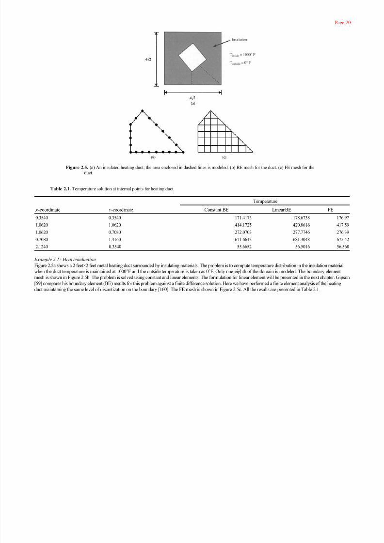
Figure 2.5. (a) An insulated heating duct; the area enclosed in dashed lines is modeled. (b) BE mesh for the duct. (c) FE mesh for theduct.
Example 2.1: Heat conduction
Figure 2.5a shows a 2 feet×2 feet metal heating duct surrounded by insulating materials. The problem is to compute temperature distribution in the insulation material
when the duct temperature is maintained at 1000°F and the outside temperature is taken as 0°F. Only one-eighth of the domain is modeled. The boundary element
mesh is shown in Figure 2.5b. The problem is solved using constant and linear elements. The formulation for linear element will be presented in the next chapter. Gipson
[59] compares his boundary element (BE) results for this problem against a finite difference solution. Here we have performed a finite element analysis of the heating
duct maintaining the same level of discretization on the boundary [160]. The FE mesh is shown in Figure 2.5c. All the results are presented in Table 2.1.
Table 2.1. Temperature solution at internal points for heating duct.
Temperature
x-coordinate y-coordinate Constant BE Linear BE FE
0.3540 0.3540 171.4173 178.6738 176.97
1.0620 1.0620 414.1725 420.8616 417.59
1.0620 0.7080 272.0703 277.7746 276.39
0.7080 1.4160 671.6613 681.3048 675.42
2.1240 0.3540 55.6652 56.5016 56.568

7/17/2019 The Boundary Element
http://slidepdf.com/reader/full/the-boundary-element 34/201
Page 21
Figure 2.6. (a) Flow around a cylinder between two parallel plates. (b) FE mesh for the flow problem domain. (c) BE mesh for the flow problem domain.
Example 2.2: Potential fluid flow
The BE program written for solving Laplace’s equation can be used to solve fluid flow problems by interpreting potential u as streamline function and the potential
gradient v=∂u/∂n as the velocity along the boundary of the problem domain. For example, consider the problem of fluid flow around a cylinder between two parallel
plates, as shown in Figure 2.6a. One quarter of the domain needs to be modeled. The boundary element mesh with linear elements is shown in Figure 2.6c. The
potential u, i.e., streamline is taken as zero at the bottom plate and the cylinder surface. The potential gradient v=∂u/∂n, i.e., the velocity along the vertical boundaries at
x=0 and x=0.6 is also zero. The fluid velocity, normal to the boundary at x=0, is assumed to be unity which will result into u=2 at the top plate. The problem is solved
by constant and linear boundary elements as well as by the finite elements. The solutions for the streamline functions at the interior points are shown in Table 2.2 for
constant as well as linear elements. The mesh used in the finite element analysis is shown in Figure 2.6b. The results from the finite element analysis are also shown in
Table 2.2. The BE and FE solutions appear to be in close agreement.
2.4. Direct method: Green’s integral theorem
The use of weighted residual technique in formulating boundary integral equations is a relatively recent development [61–63]. Classical approaches utilized Green’s
integral identities in order to derive boundary integral equations. Let us consider two functions and ψ defined in the domain Ω of Figure 2.7. Suppose that these
functions and their first partial derivatives are continuous in the domain. Green’s second integral identity involving these functions and their derivatives can be written as:
(2.31)

7/17/2019 The Boundary Element
http://slidepdf.com/reader/full/the-boundary-element 35/201
Page 22
Figure 2.7. Integration over a small circular boundary Γε.
Table 2.2. Streamline solution at interior points for fluid flow.
FE Nodes x-coord. y-coord. Constant BE Linear BE Finite element
34 2.16E−01 6.99E−02 6.95E−01 6.95E−01 0.69672
35 1.08E−01 7.07E−02 7.06E−01 7.06E−01 0.70639
36 1.02E−01 1.51E−01 1.51E+00 1.51E+00 1.5067
37 3.24E−01 7.22E−02 6.99E−01 6.99E−01 0.70334
38 1.59E−01 1.40E−01 1.39E+00 1.39E+00 1.3939
39 3.85E−01 9.74E−02 9.10E−01 9.09E−01 0.90688
40 3.66E−01 1.48E−01 1.45E+00 1.45E+00 1.447
41 3.07E−01 1.39E−01 1.38E+00 1.38E+00 1.3755
42 2.33E−01 1.37E−01 1.37E+00 1.37E+00 1.366
43 4.38E−01 1.15E−01 1.01E+00 1.01E+00 1.0118
44 5.03E−01 1.69E−01 1.55E+00 1.55E+00 1.5496
45 4.62E−01 1.63E−01 1.53E+00 1.53E+00 1.5328
46 4.17E−01 1.56E−01 1.50E+00 1.50E+00 1.5013
47 5.25E−02 1.60E−01 1.60E+00 1.60E+00 1.5971
48 6.27E−02 1.06E−01 1.06E+00 1.06E+00 1.0588
49 5.35E−01 1.75E−01 1.59E+00 1.60E+00 1.5881
50 5.43E−01 1.55E−01 1.27E+00 1.28E+00 1.2569
51 5.37E−01 1.08E−01 5.08E−01 5.12E−01 0.49792
52 5.04E−01 9.65E−02 5.52E−01 5.52E−01 0.54674
53 4.82E−01 1.28E−01 1.05E+00 1.05E+00 1.0445
54 4.16E−01 5.49E−02 4.64E−01 4.64E−01 0.47171
55 5.69E−01 1.53E−01 1.17E+00 1.19E+00 1.165
56 5.66E−01 1.33E−01 8.19E−01 8.46E−01 0.8088
57 5.69E−01 1.13E−01 4.05E−01 4.36E−01 0.38894
58 5.67E−01 1.75E−01 1.57E+00 1.58E+00 1.5606
59 3.85E−02 1.28E−01 1.28E+00 1.28E+00 1.2817
60 4.68E−01 7.91E−02 5.48E−01 5.49E−01 0.54814
61 5.26E−01 1.39E−01 1.05E+00 1.05E+00 1.043

7/17/2019 The Boundary Element
http://slidepdf.com/reader/full/the-boundary-element 36/201
Page 23
We can identify the functions (Fig. 2.7). Green’s second integral identity can be applied to the region Ω−Ωε:
Note that both boundaries of the region Ω−Ωε, viz., Γ and Γ
ε, are included in writing the integral identity. The left-hand side of this equation is identically zero. Let us
evaluate the first integral on the right-hand side on the boundary Γε:
The second integral on the boundary Γε would vanish in the limit as ε→0. Thus, equation (2.32) becomes:
This equation states that a harmonic function at a point p(u p ) in the domain Ω can be expressed as the sum of a single-layer potential (integral term with the fundamental
solution, u*, in it) with density ∂u/∂n and a double-layer potential (integral term with the normal derivative of the fundamental solution, ∂u*/∂n, in it) with density— u.We note here that the single-layer potential is continuous, but the double-layer potential experiences a jump as the point p passes through the boundary of the domain.
It can be seen that equation (2.34) is essentially identical to equation (2.10) derived using the weighted residual method. The limits for specializing the interior point p to
the boundary, leading to equation (2.19), can be taken in the same way as in Section 2.2. We will use weighted residual technique in the rest of the book for deriving
boundary element equations.
The materials presented up to this point in this chapter would be adequate for a general understanding of the fundamentals of the boundary element formulation. Very
often the approach outlined thus far would be found in boundary element literature that describes the basic methodology. The next section on indirect method,
therefore, is presented briefly for the sake of completeness.
2.5. Indirect method
In the direct method, the physical quantities themselves are used as the unknown variables to be solved by numerical means. For example, the harmonic function u and
its normal derivative v, defined in Sections 2.2 and 2.4, are solved as unknowns in the direct method. Depending on the physical problem solved, these harmonic
functions may represent temperature or velocity of flow or electrical volt. In the so-called semi-direct method, which also uses the direct formulation as derived in
Sections 2.2
(2.32)
(2.33a)
(2.33b)
(2.34).

7/17/2019 The Boundary Element
http://slidepdf.com/reader/full/the-boundary-element 37/201
Page 24
and 2.4, the unknown function may be taken as the stress function or stream function or magnetic potential function. The physical quantities of the problem at hand can
be computed by differentiation of these functions after the unknowns have been solved for using BEM. In the indirect or source method, however, “source” densities
are used as the unknowns of the problem. These source densities may or may not have any direct physical meaning for the problem to be solved. The physical
quantities are computed using integral expressions in terms of the source densities after the source densities have been solved for.
We have seen from equation (2.34) that a harmonic function at any point in the domain can be expressed as the sum of a single-layer potential with an unknown
density and a double-layer potential with another unknown density. Suppose the entire boundary of the problem is of the Dirichlet type, i.e., Γu
. In that case the
unknown harmonic function u(p) may be expressed only by a double-layer potential of unknown density σ(Q):
Since we already know that the double-layer potential experiences a jump as the domain point p approaches the boundary point P, we obtain from equation (2.35)
(along the same line of derivation used for eqn. 2.18):
In equation (2.36) the boundary at the source point P has been assumed to be smooth. This is a Fredholm integral equation of the second kind. Alternatively, Dirichlet
boundary value problem can be solved by expressing the unknown harmonic function u(p) only as a single-layer potential with unknown density σ(Q):
As p approaches P, unlike the double-layer potential, the single-layer potential does not experience a jump. Thus, equation (2.37) becomes:
This is a Fredholm integral equation of the first kind. Equations of this type are more difficult to solve, compared to Fredholm equation of the second kind, because of
possible ill-conditioning of the matrices and non-uniqueness of the solution resulting from the discretization of the problem [16].
For the Neumann problem, i.e., if the entire boundary is of the type Γv , we can assume that the unknown harmonic function u(p) may be expressed solely as a
single-layer potential with unknown density σ(Q):
(2.35)
(2.36)
(2.37)
(2.38)
(2.39)

7/17/2019 The Boundary Element
http://slidepdf.com/reader/full/the-boundary-element 38/201
Page 25
Taking directional derivative of the function u(p) at a point p in the normal direction n to the boundary we get:
If we take the limit as the internal point p approaches the boundary point P, we obtain the following integral equation:
This is a Fredholm integral equation of the second kind. Once again, the boundary at the point P is assumed to be smooth. Equation (2.41) will have a solution if the
following relation, known as the Gauss condition, is satisfied [60]:
The solution to equation (2.41) is unique only up to an arbitrary additive constant. A unique solution to equation (2.41) can, however, be obtained by imposing some
normalization procedure [62].
For the boundary value problem having mixed Dirichlet and Neumann boundary conditions, one can proceed as in the pure Neumann problem and express the
function u(p) as a single-layer potential:
The constant is added to ensure uniqueness of the solution. Once again, taking a directional derivative, one obtains:
As the domain point p approaches the boundary point P, equations (2.43) and (2.44) take the form:
This equation pair is solved simultaneously for the unknown source density σ on the boundary. The unknown function, u, on the boundary Γv
and the unknown normal
derivative, v, of the function on the boundary Γu
can then be computed using the following equations:
(2.40)
(2.41)
(2.42)
(2.43)
(2.44)
(2.45)
(2.46)
(2.47)
(2.48)

7/17/2019 The Boundary Element
http://slidepdf.com/reader/full/the-boundary-element 39/201
Page 26
2.6. Body forces
The problems that can be solved using boundary element formulation presented in all of the previous sections are driven solely by the boundary conditions. In many
practical applications, the domain may contain discrete or distributed sources or body forces, such as, heat generation for heat conduction problem or electrical charges
for electrostatic problem. This type of problem is governed by the Poisson’s equation:
where “b” is the source term. Depending on the type of the source, a number of strategies may be employed to include the effects of the domain term “b”.
First, we can transform the boundary-value problem for the Poisson’s equation into one for the Laplace’s equation by subtracting a particular solution that is
independent of the boundary conditions. Suppose we are required to solve the problem: with uc
=−u p
on Γ.
Second, for many practical cases it will be difficult to find a particular solution. For example, the values of “b” may be provided in a tabular form applied at a series
of points in Ω. In these situations, the boundary element formulation given by equation (2.19) can be extended to include the domain term “b” in the following manner:
The domain term can be computed by dividing the domain Ω into a number of internal cells (Fig. 2.8) and performing numerical integration over these cells. A typical
term corresponding to a source point “i” on the boundary Γ can be written as:
Figure 2.8. Internal cells for domain term integration.
(2.49)
(2.50)
(2.51)

7/17/2019 The Boundary Element
http://slidepdf.com/reader/full/the-boundary-element 40/201
Page 27
where N c
is the total number of internal cells, N i is the number of integration points in each cell, w
k are the integration weights and A
l is the area of the “l”th cell. The
entire system of equations for the N boundary elements corresponding to equation (2.25) can now be written as:
The discretization of the domain Ω into a number of cells for evaluating the domain term does not introduce any extra unknown into the system of equations. Thus,
applying boundary conditions the above set of equations can be rearranged into a system similar to equation (2.27). After this set of equations has been solved, the
values of u and v will be known over the entire boundary Γ. The value of the function u at any interior point “i”, similar to equation (2.28), can then be computed usingthe following equation:
Third, if the body term “b” is a harmonic function, i.e., if and then apply Green’s second identity in the following fashion:
Since we assumed that , we obtain:
One form of function U* that satisfies the relation is given by:
If we substitute the expression (2.55) into equation (2.50), we see that all the terms are now applied on the boundary only.
Fourth, if there are a number of concentrated sources “Q” at discrete interior points of the domain Ω in addition to the distributed sources “b”, equation (2.50)
can be modified to include the effects of the sources:
Example 2.3: Twist of a prismatic shaft
The governing differential equation for the twist of a homogeneous prismatic shaft in terms of the stress function u is given as:
where G is the shear modulus and θ is rate of twist. The shear stresses can be derived from the stress function. The stress function is constant (for convenience it is
assumed
(2.52)
(2.53)
(2.54)
(2.55)
(2.56)
(2.57)
(2.58)

7/17/2019 The Boundary Element
http://slidepdf.com/reader/full/the-boundary-element 41/201
Page 28
Figure 2.9. (a) FE mesh of the elliptical section of the shaft. (b) BE mesh of the elliptical section.
Table 2.3. Solution of stress function for twist of a shaft.
x-coord y-coord Exact solution Constant BE Linear BE Finite element
0.0 0.0 0.8 0.798 0.803 0.793
0.35 0.0 0.7755 0.773 0.778 0.782
1.0 0.0 0.6 0.599 0.602 0.5911.5 0.0 0.35 0.358 0.351 0.347
0.0 −0.44 0.64512 0.644 0.648 0.681
0.6 −0.44 0.57312 0.571 0.576 0.569
1.2 −0.44 0.35712 0.355 0.359 0.336

7/17/2019 The Boundary Element
http://slidepdf.com/reader/full/the-boundary-element 42/201
Page 29
to be zero) on the boundary. Let G=θ =1. Also, let us consider a prismatic shaft of elliptic cross section:
Let us take a=2 and b=1 for this example [69]. The problem is solved by the boundary element and finite element methods (FEMs). For the finite element analysis, 33
nodes and 48 linear triangular elements are used (Fig. 2.9a) and 16 constant/linear elements are used for the boundary element analysis (Fig. 2.9b). For the BE
analysis, the finite elements of Figure 2.9a are used as the internal cells to integrate the domain term. The results of the analyses for a few internal points are presented in
Table 2.3. The exact solutions at these internal points are also shown in the table.
(2.59)

7/17/2019 The Boundary Element
http://slidepdf.com/reader/full/the-boundary-element 43/201

7/17/2019 The Boundary Element
http://slidepdf.com/reader/full/the-boundary-element 44/201
Page 31
Chapter 3
Isoparametric Boundary Elements
3.1. Introduction
The fundamentals of the boundary element method (BEM) were presented in Chapter 2. The reader may notice that if the solution variables are represented asconstants over the boundary segments, the developments of Chapter 2 are sufficient for an understanding and implementation of the method. However, for better
representation of the geometry as well as better accuracy of the solution variables, often, higher polynomial order representation of the solution variables as well as the
geometry is needed. As in the finite element methods (FEM), this leads to isoparametric formulation of the boundary element equations. This chapter will present the
basic approach of transforming the global coordinates to normalized local systems and the use of higher order polynomial shape functions in the process of boundary
element discretization.
3.2. Two-dimensional linear boundary elements
As in the case of constant boundary element, which was developed in the previous chapter, the boundary curve Γ is once again divided into “N” small straight
boundary element segments (Fig. 3.1). Unlike in the constant elements, the unknown function u and its normal derivative v are assumed to vary linearly over each
element segment. The nodes are located at the ends of the element segment. It means that adjacent elements share nodes, ensuring inter-element continuity of the
function u and its normal derivative v. The angle α p
of Figure 2.2 can no longer be assured to equal to 180°. For the discretized boundary, the equation (2.19) can be
written for the i-th source point in the following fashion:
We will shortly show a simple technique to compute the coefficient C i. The unknown function u and its normal derivative v can no longer be pulled out of the integral
sign because they vary linearly over the element segment. A linear boundary element is shown in Figure 3.2 along with the functional variation of u and v. These
functions
(3.1)
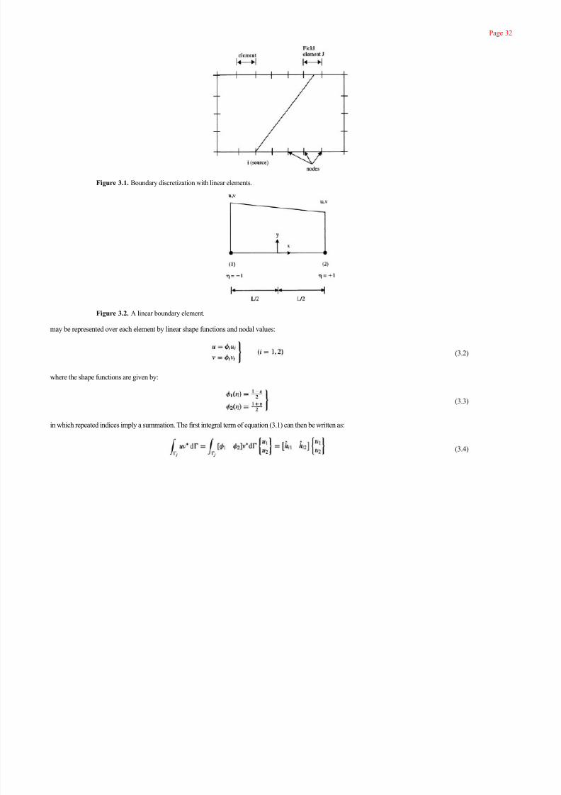
7/17/2019 The Boundary Element
http://slidepdf.com/reader/full/the-boundary-element 45/201
Page 32
Figure 3.1. Boundary discretization with linear elements.
Figure 3.2. A linear boundary element.
may be represented over each element by linear shape functions and nodal values:
where the shape functions are given by:
in which repeated indices imply a summation. The first integral term of equation (3.1) can then be written as:
(3.2)
(3.3)
(3.4)

7/17/2019 The Boundary Element
http://slidepdf.com/reader/full/the-boundary-element 46/201
Page 33
with:
Similarly, the second term of equation (3.1) can be written as:
with:
The assembled equation for the source point “i” can thus be easily written as:
where, Ĥ i1=(ĥ i1 from element“j”)+(ĥ i2 from element “ j−1”). Similarly, Gi1=( g i1 from element“j”)+( g i2 from element “ j−1”). The equation (3.8) can be written in a
concise form as follows:
In matrix form this will lead to equation (2.25). However, equation (2.26) will now take the form:
where [C] is a diagonal matrix whose coefficients are evaluated using a procedure shown below. As in the constant element, we can use Gaussian quadrature for the
non-singular elements. Any source point “i” is connected to two adjacent elements “i−1” and “i”, as shown in Figure 3.3. All four ĥ ij terms, two for the (i−1)th
element and another two for the (i)th element, will equal to zero, as r · n=0. The corresponding g ij terms can be evaluated analytically. The results are recorded below:
(3.5)
(3.6)
(3.7)
(3.8)
(3.9)
(3.10)
(3.11)
(3.12)

7/17/2019 The Boundary Element
http://slidepdf.com/reader/full/the-boundary-element 47/201
Page 34
Figure 3.3. Linear singular boundary elements.
Evaluation of the jump term in equations (3.9) and (3.10)
It was mentioned earlier that the jump term C i of equation (3.9) or (3.10) can be calculated in a simple way. Here we describe the procedure. We apply a uniform
potential u over the whole boundary. Then, the v values are zero. Equation (2.25) becomes:
Since u is uniform, the sum of all the elements of [H] in any row ought to be zero. Hence,
So, the diagonal of matrix [H] can be computed indirectly without resorting to a geometric evaluation of the coefficient C i. Once again, the application of appropriate
boundary conditions to equation (2.25) will lead to equation (2.27).
3.3. Higher-order elements in 2-D
The formulation developed in the previous section can be systematically extended to quadratic and higher-order boundary elements. Higher-order boundary elements
may be useful (a) to represent the geometry more accurately and (b) to obtain more accurate results for the solution variables. One can start from the discretized
equation (3.1). The unknown quantities u and v will now be quadratic or higher-order functions of the coordinate η defined over the transformed domain (−1, 1). For
the quadratic boundary elements (Fig. 3.4), these functions are written as:
(3.13)
(3.14)

7/17/2019 The Boundary Element
http://slidepdf.com/reader/full/the-boundary-element 48/201
Page 35
Figure 3.4. Quadratic boundary element and its transformation.
The quadratic shape functions are given by:
In order to represent the differential boundary segment dΓ in terms of the coordinate η, the geometric coordinates x and y are also expressed using the shape functions
of equation (3.15):
The differential boundary segment dΓ can now be written as:
where, the Jocobian of transformation |G|, is given by:
Thus, the integral involving the function u of the boundary element equation (3.1) becomes:
The integrals involving the function q can be dealt with in the same fashion.
(3.15)
(3.16)
(3.17)
(3.18)
(3.19)
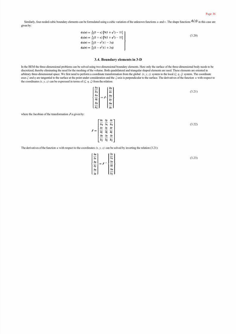
7/17/2019 The Boundary Element
http://slidepdf.com/reader/full/the-boundary-element 49/201
Page 36
Similarly, four-noded cubic boundary elements can be formulated using a cubic variation of the unknown functions u and v. The shape functions in this case are
given by:
3.4. Boundary elements in 3-D
In the BEM the three-dimensional problems can be solved using two-dimensional boundary elements. Here only the surface of the three-dimensional body needs to be
discretized, thereby eliminating the need for the meshing of the volume. Both quadrilateral and triangular shaped elements are used. These elements are oriented in
arbitrary three-dimensional space. We first need to perform a coordinate transformation from the global (x, y, z) system to the local (ξ, η, ζ) system. The coordinate
axes ξ and η are tangential to the surface at the point under consideration and the ζ -axis is perpendicular to the surface. The derivatives of the function u with respect to
the coordinates (x, y, z) can be expressed in terms of (ξ, η, ζ) from the relation:
where the Jacobian of the transformation J is given by:
The derivatives of the function u with respect to the coordinates (x, y, z) can be solved by inverting the relation (3.21):
(3.20)
(3.21)
(3.22)
(3.23)

7/17/2019 The Boundary Element
http://slidepdf.com/reader/full/the-boundary-element 50/201
Page 37
The typical boundary integral terms that need to be evaluated are:
The differential area dS can be expressed in terms of the local coordinates (ξ, η, ζ). If r is the position vector of a point on the surface of the body, then dS is given by:
The vector cross product yields a vector that is perpendicular to the surface, i.e., along the ζ -axis and |G | is the magnitude of this normal. The derivatives ∂r /∂ξ and
∂r /∂η are written as:
The normal vector n can be computed from the vector cross product:
with the components:
The magnitude of n is then computed as:
The integrals of equation (3.24) are then converted to:
The expression for a differential volume, dΩ can be obtained from a vector box product:
which is utilized in evaluating the body load domain integral term of the equation (2.50):
(3.24)
(3.25)
(3.26)
(3.27)
(3.28)
(3.29)
(3.30)
(3.31)
(3.32)

7/17/2019 The Boundary Element
http://slidepdf.com/reader/full/the-boundary-element 51/201
Page 38
Figure 3.5. Four-noded quadrilateral boundary element and its transformation.
The above coordinate transformation allows one to develop three-dimensional boundary elements. The formulation for quadrilateral and triangular boundary elements is
presented in the following sections.
3.4.1. Quadrilateral elements The quadrilateral elements can be defined by four nodal points (Fig. 3.5) with bilinear variation of the unknown functions u and v. These functions as well as the
coordinates (x, y, z) are expressed, much the same way as in equations (3.14) and (3.16), using shape functions and nodal values of the unknown functions ui
(or vi) or coordinates x
i (or y
i or z
i). To facilitate numerical integration, the shape functions are chosen such that the quadrilateral defined by the nodal coordinates
[(x1 , y
1 ) (x
2 , y
2 ), (x
3 , y
3 ), (x
4 , y
4 )] is mapped on to a domain in the (ξ, η) plane with the transformed nodal coordinates [(−1, −1), (1, −1), (1, 1), (−1, 1)]. The shape
functions for the quadrilateral boundary elements are given by:
All the functions of the equations, (3.30) and (3.32) can now be evaluated at the Gaussian quadrature points.Higher-order quadrilaterals can also be defined using more nodes and shape functions. For example, we can define an eight-noded serendipity quadrilateral element
or a nine-noded Lagrangian quadrilateral element. The derivatives of the unknown
(3.33)

7/17/2019 The Boundary Element
http://slidepdf.com/reader/full/the-boundary-element 52/201
Page 39
Figure 3.6. Eight-noded serendipity quadrilateral boundary element.
functions can also be used as nodal degrees of freedom. The shape functions for the eight-noded serendipity quadrilateral element (Fig. 3.6) are given below:
3.4.2. Triangular elements
A triangular boundary element can be defined by three nodal points (Fig. 3.7). A local oblique coordinate system (ξ, η) is defined at the nodal point 3. The local vectors
e1
and e2 , defined along ξ and η, respectively, can be expressed in terms of the global unit vector triad (i, j, k):
(3.34)
(3.35)
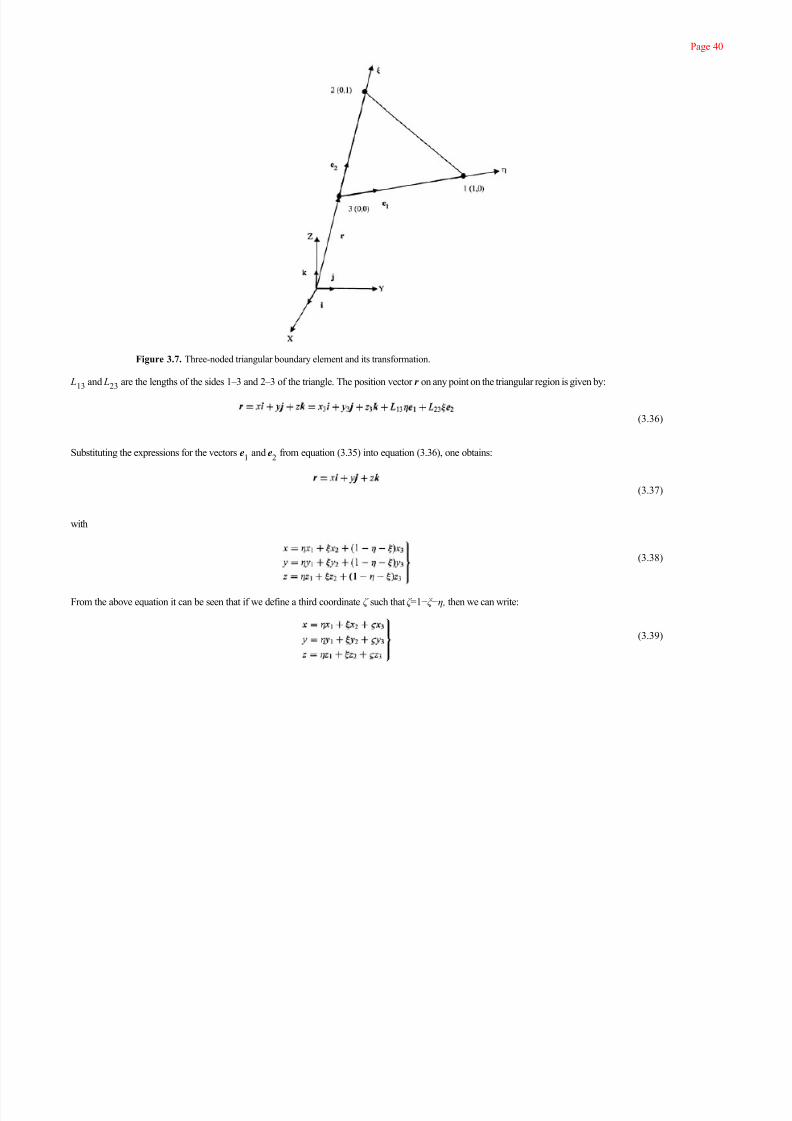
7/17/2019 The Boundary Element
http://slidepdf.com/reader/full/the-boundary-element 53/201
Page 40
Figure 3.7. Three-noded triangular boundary element and its transformation.
L13
and L23
are the lengths of the sides 1–3 and 2–3 of the triangle. The position vector r on any point on the triangular region is given by:
Substituting the expressions for the vectors e1
and e2
from equation (3.35) into equation (3.36), one obtains:
with
From the above equation it can be seen that if we define a third coordinate ζ such that ζ =1−ξ −η, then we can write:
(3.36)
(3.37)
(3.38)
(3.39)

7/17/2019 The Boundary Element
http://slidepdf.com/reader/full/the-boundary-element 54/201
Page 41
which can be written in matrix form:
Since ζ is not an independent coordinate, we can only invert the first two equations:
The coordinate ζ is obtained from the relation ζ =1−ξ −η, yielding
The expressions for αi , β
i and A
i can be obtained from the following recursive relations:
The area of the triangle A is computed as:
This area is the projection of the triangular element on to the (x, y) plane. It is obvious from equations (3.39) that the interpolation functions in this case are simply the
local coordinates ( ). Thus,
Because of the use of local coordinates (ξ, η, and ζ ) the necessary integrals can be performed here in closed form:
The shape functions for the six-noded second-order triangular elements (Fig. 3.8) are given as follows:
(3.40)
(3.41)
(3.42)
(3.43)
(3.44)
(3.45)
(3.46)
(3.47)

7/17/2019 The Boundary Element
http://slidepdf.com/reader/full/the-boundary-element 55/201
Page 42
Figure 3.8. Six-noded serendipity triangular boundary element.
3.5. Examples
A number of example problems are presented in this section illustrating the use of lower and higher order boundary elements in 2-D and 3-D. For simplicity, the
theoretical developments of this and last chapter were confined to potential problems only. The formulations presented so far are however expandable to elasticity or
acoustics. Although we are postponing the development of detailed boundary element formulations for elasticity and acoustics till later chapters, we present two
elasticity problems in this section. These elastostatic stress analysis problems are designed to demonstrate the use and performance of higher order boundary elements.
Example 3.1: Flow of perfect fluid around aerofoils
In this example we will study the flow of a perfect fluid past an aerofoil designated as NACA 0018. The flow can be indirectly described by a stream function u, which
is related to the velocities in the following manner:
The far field velocities away from the aerofoil are given as:
The stream function u can be separated into two components:
where u1
is the free flow stream function in the absence of the aerofoil and u2
is the stream function for perturbed flow. Thus, u1
=V y
. If we consider the total stream
function u=0 on the aerofoil surface Γ, then
(3.48)
(3.49)
(3.50)
(3.51)

7/17/2019 The Boundary Element
http://slidepdf.com/reader/full/the-boundary-element 56/201
Page 43
Figure 3.9. Boundary element discretization of NACA 0018 aerofoil.
Due to symmetry we only need to discretize one-half of the aerofoil (Fig. 3.9). Table 3.1 shows the tangential velocity, normalized to V, as a function of x-coordinate
solved using linear boundary elements. The solution produced by NACA is also shown in the table [69].
Example 3.2: Heat conduction in an infinite medium
Consider a spherical cavity of unit radius placed in an infinite conducting medium [71]. A constant radial flux of 10 J/(m 2s) is prescribed over the surface of the cavity.
The temperature distribution in the infinite medium can be computed using 3-D boundary element discretization. Unlike the FEM, here only the surface of the cavity is
required to be discretized. Due to symmetry, only one-eighth of the cavity surface is modeled using flat triangular elements with constant potential and normal derivative.
Unlike finite methods, the use of constant field variables and its normal derivatives on the element segment is commonplace in the boundary element literature. The inter-
element discontinuities in solution variables are mitigated by the fact that BEM is an integral equation technique and tends to average out errors arising out of
discontinuities.
Table 3.1. Tangential velocity of flow around NACA 0018 aerofoil.
Solution for v/V (v=tangential velocity)
x-coordinate Analytical solution Boundary element solution
0.0 0.000 0.000
1.25 0.926 0.931
2.5 1.103 1.093
5.0 1.228 1.212
7.5 1.267 1.253
10.0 1.276 1.265
15.0 1.278 1.273
20.0 1.275 1.269
25.0 1.262 1.25430.0 1.247 1.236
40.0 1.205 1.198
50.0 1.157 1.158
60.0 1.116 1.118
70.0 1.074 1.079
80.0 1.025 1.036
90.0 0.966 0.975
95.0 0.914 0.941
100.0 0.000 0.000

7/17/2019 The Boundary Element
http://slidepdf.com/reader/full/the-boundary-element 57/201
Page 44
Figure 3.10. (a) Boundary element surface mesh and (b) finite element 3-D mesh of thick cylinder.
Results, produced using constant elements, are presented in Table 3.2, where averaged temperatures on the cavity surface and temperature distribution inside the
infinite medium are shown. The exact solution for this problem is given by u=10/ R, where R is the radial distance ( R≥1). The exact solutions are also given in the table.
The boundary element (BE) solution would converge at a faster rate to the exact solution if higher order boundary elements were employed.
Example 3.3: Internally pressurized thick cylinder
A thick cylinder of length h=40 mm, having inner and outer diameters a=10 mm and b=20 mm respectively, is subjected to internal pressure p=20 N/mm2. The
Young’s modulus E =210000 N/mm2 and Poisson’s ratio υ=0.3 for the cylinder material. A 90° sector is modeled using (a) linear boundary element, (b) quadratic
boundary element and (c) finite element [63]. The finite element and boundary element meshes are shown in Figure 3.10. A 20-noded serendipity element is used for
finite element discretization.
Table 3.2. Temperature distribution in an infinite medium from a spherical cavity.
BEM
R ( N =7) ( N =16) Exact
1.0 9.676 9.727 10.000
1.5 6.505 6.569 6.667
2.0 4.899 4.922 5.000
3.0 3.274 3.281 3.333
6.0 1.639 1.640 1.667
10.0 0.983 0.984 1.000
100.0 0.098 0.098 0.100
1000.0 0.010 0.010 0.010
( N =number of boundary element segments).

7/17/2019 The Boundary Element
http://slidepdf.com/reader/full/the-boundary-element 58/201
Page 45
Figure 3.11. Schematic of the gear tooth. a=2.00 mm, b=16.00 mm, c=5.70 mm, d =18.25 mm, e=17.25 mm, R (radius)=31.25 mm.
A four-noded surface element and an eight-noded serendipity surface element are used for the linear and quadratic boundary element models respectively. In the case
of boundary element solution, the numerical integration points were concentrated near singularities to achieve better accuracy [63].
Table 3.3. Displacements and stresses in internally pressurized thick cylinder.
Boundary element solution
Function Radius Exact solution Finite element solution Linear BE Quadratic BE
Radial displacement 10.012.515.017.520.0
1.9041.6021.4151.2931.212
1.9051.6001.4141.2921.212
1.8181.5681.3191.2341.150
1.9051.6001.4141.2911.211
Radial stress 10.012.515.017.520.0
−20.0−10.4
−5.2−2.0
0.0
−17.4−11.6
−3.5−2.4
0.7
−13.8−13.2
−1.8−1.2
1.1
−18.5−11.3
−4.1−2.2
0.4
Hoop stress 10.012.515.017.520.0
33.323.718.515.413.3
34.423.319.215.213.5
27.120.115.214.312.1
33.523.718.515.413.3
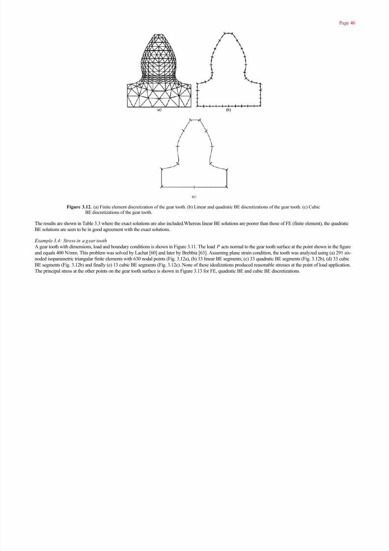
7/17/2019 The Boundary Element
http://slidepdf.com/reader/full/the-boundary-element 59/201
Page 46
Figure 3.12. (a) Finite element discretization of the gear tooth. (b) Linear and quadratic BE discretizations of the gear tooth. (c) CubicBE discretizations of the gear tooth.
The results are shown in Table 3.3 where the exact solutions are also included.Whereas linear BE solutions are poorer than those of FE (finite element), the quadratic
BE solutions are seen to be in good agreement with the exact solutions.
Example 3.4: Stress in a gear tooth
A gear tooth with dimensions, load and boundary conditions is shown in Figure 3.11. The load P acts normal to the gear tooth surface at the point shown in the figure
and equals 400 N/mm. This problem was solved by Lachat [60] and later by Brebbia [63]. Assuming plane strain condition, the tooth was analyzed using (a) 291 six-
noded isoparametric triangular finite elements with 630 nodal points (Fig. 3.12a), (b) 33 linear BE segments, (c) 33 quadratic BE segments (Fig. 3.12b), (d) 33 cubic
BE segments (Fig. 3.12b) and finally (e) 13 cubic BE segments (Fig. 3.12c). None of these idealizations produced reasonable stresses at the point of load application.The principal stress at the other points on the gear tooth surface is shown in Figure 3.13 for FE, quadratic BE and cubic BE discretizations.

7/17/2019 The Boundary Element
http://slidepdf.com/reader/full/the-boundary-element 60/201
Page 47
Figure 3.13. Principal stresses at the surface of the gear tooth.

7/17/2019 The Boundary Element
http://slidepdf.com/reader/full/the-boundary-element 61/201
Page 48
This page intentionally left blank.

7/17/2019 The Boundary Element
http://slidepdf.com/reader/full/the-boundary-element 62/201
Page 49
Chapter 4
Anisotropy, Axisymmetry and Zoning
4.1. Introduction
Unlike the finite elements, the boundary element method (BEM) requires relatively more analytical work to formulate the numerical equations in the case ofaxisymmetric bodies and when the material anisotropy needs to be considered.
When the solution domain contains inhomogeneity, it can be handled in BEM by partitioning the domain into zones having homogeneous properties. As an added
benefit, zoning produces banded system matrix thereby making the problem suitable for banded matrix solvers. We will see in later chapters that zoning helps improve
the solution accuracy, especially when dealing with acoustic eigenvalue analysis of chunky-type enclosures.
4.2. Anisotropic materials
At times engineering materials and media cannot be adequately described using isotropic material properties. The materials may respond differently in orthogonal
directions (orthotropic behavior) or in all directions (anisotropic behavior). In this section, we shall present necessary ingredients which will allow us to formulate
boundary integral equations in these cases.
Orthotropic materials
Consider the domain shown in Figure 4.1 with x and y being the directions of orthotropy. The Laplace’s equation in this case is given by:
where k x , k
y and k
z are the material properties in the x, y and z directions, respectively. The fundamental solutions to these equations are:
(4.1)
(4.2)
(4.3)
(4.4)

7/17/2019 The Boundary Element
http://slidepdf.com/reader/full/the-boundary-element 63/201
Page 50
Figure 4.1. A Two-dimensional orthotropic medium ( x & y are directions of orthotropy).
respectively, where:
It would also be necessary to define boundary fluxes v and v*. To this end, we apply the divergence theorem to the left-hand side of equation (4.1):
where n x
and n y
are direction cosines and the quantity between the brackets on the right-hand side is the normal boundary flux:
We can analogously define v* as:
The corresponding quantities in three-dimensions can easily be defined. Using the governing equation (4.1) or (4.2) and given boundary conditions, we can formulate
the boundary integral equation in the same fashion as in the isotropic case and arrive at a formulation similar to equation (2.19).
(4.5)
(4.6)
(4.7)
(4.8)
(4.9)

7/17/2019 The Boundary Element
http://slidepdf.com/reader/full/the-boundary-element 64/201
Page 51
Anisotropic materials
If the medium is anisotropic with the material property coefficients given by k ij , the governing differential equation in two dimensions can be written as:
The fundamental solution for this equation is:
where |k ij
| is the determinant of the material property coefficient matrix and “r” is given by:
The quantities v and v* are respectively given by:
The problem can be formulated as in the previous case.
4.3. Axisymmetric problems
Three-dimensional boundary value problems having axial symmetry in geometry, loading and boundary conditions can be solved in two dimensions, thereby saving
significant efforts. A body with symmetry about the Z -axis is shown in Figure 4.2. In the BEM we only need to discretize the contour lines Γ b
. Thus, three-dimensional
axisymmetric problems can be solved using line elements. To this end, the boundary integral equation (2.19) is written in cylindrical polar coordinate system ( R, Θ, Z )
with the fundamental solution u* of equation (2.9) also expressed in the same coordinate system. Taking advantage of axial symmetry, the dependence on Θ is then
integrated out. The final equation is given in the (R–Z) plane:
in which the fundamental solution u* and its normal derivative v* are given by:
(4.10)
(4.11)
(4.12)
(4.13)
(4.14)
(4.15)
(4.16)

7/17/2019 The Boundary Element
http://slidepdf.com/reader/full/the-boundary-element 65/201
Page 52
Figure 4.2. Axisymmetric body. Ω is the generating area and Γ b
is the boundary contour.
K(κ) and E(κ) are the complete elliptic integral of the first and second kinds respectively. The argument κ is given by:
In equation (4.17), nr (Q) and n z (Q) are the R- and Z -components of the outward normal at the boundary field point Q. Note that the fundamental solution [eqn.(4.16)] in the axisymmetric case is a function of the distances of the source and field points P and Q from the axis of revolution Z . Recall that the fundamental solutions
for the two-and three-dimensional cases [eqns. (2.8) and (2.9)] are given simply as a function of distance between the source and field points r(P, Q). The solution of
the equation (4.15) can be approached in the same fashion as was done in the case of the boundary element equation (2.18). The boundary contour Γ b
of the
axisymmetric body of Figure 4.2 can be divided into a number of line segments. Numerical integration is then performed
(4.17)
(4.18)

7/17/2019 The Boundary Element
http://slidepdf.com/reader/full/the-boundary-element 66/201
Page 53
Figure 4.3. BE discretization of the axisymmetric solid cylinder.
on each line segment and contributions are assembled into a system of equation, which is of the form of equation (2.25).
When the source point P does not lie on or is close to an element segment, numerical integrals can be performed using a standard Gaussian quadrature. The valuesof the complete elliptic integrals can be incorporated into the computer program in tabular form as a function of their argument κ . For a computed value of the argument
κ at a Gaussian point, the values of the complete integrals can be looked up from this table. However, the elliptic integrals can also be approximated by polynomial
expressions [163]. For the evaluation of the integrals on the singular elements, the fundamental solution u* and its normal derivative v* are expressed in terms of
Legendre functions of the second kind [71]. The integration can then be performed analytically by expanding these Legendre functions [164]. Furthermore, when r(P)
is small, i.e., when the element is located near the axis of revolution, the integration must be performed with care [71,165].
Example 4.1: Heat conduction in a solid axisymmetric cylinder
Consider a solid axisymmetric cylinder with 0≤ R<a and 0< Z <l [71]. Specified boundary conditions are given as: u=0 at Z =l,u=1 at Z =0 and v+hu=0 at R=a. The
surface at R=a has a convection boundary condition where h is the heat transfer coefficient. For this example, we assume a=1, l =3 and h=0.1. In order to solve this
problem by the BEM, only the surfaces at Z =0, Z =l and R=a need to be discretized. A total of 20 equal-length linear boundary elements are used for this purpose (Fig.
4.3). Results are presented in Table 4.1 where exact solutions are also shown.

7/17/2019 The Boundary Element
http://slidepdf.com/reader/full/the-boundary-element 67/201
Page 54
Figure 4.4. A domain is divided into two sub-regions (zones).
4.4. Inhomogeneous regions and zoning
In many practical engineering applications, the problem may only be piecewise homogeneous or the domain may have an irregular shape having one of the dimensions
much larger than others. In these cases, the domain is divided into regular homogeneous subregions. The boundary element equations are derived independently for
each subregion. These equations can be assembled into a single set of equations for the whole body using the compatibility and equilibrium conditions on the interface
between the subregions.
Let us consider a Ω domain, which is divided into two different subregions Ω1
and Ω2
as shown in Figure 4.4. For the subregion 1, the boundary element equations
can be written as:
The equations for the subregion 2 can similarly be written as:
where:
u1 , v
1=nodal potentials and fluxes on Γ1
.
u2 , u
2=nadal potentials and fluxes on Γ2
.
=nadol potentials and fluxes on ΓI with respect to the subregion Ω
1.
=nadol potentials and fluxes on ΓI with respect to the subregion Ω
2.
Table 4.1. Temperature distribution in a solid axisymmetric cylinder.
z BE solution ( R=0.25) Exact solution ( R=0.25) BE solution ( R=1.00) Exact solution ( R=1.00)
0.5 0.781 0.781 0.751 0.751
1.0 0.585 0.585 0.560 0.560
1.5 0.416 0.416 0.397 0.397
2.0 0.267 0.267 0.254 0.254
2.5 0.130 0.130 0.124 0.124
(4.19)
(4.20)

7/17/2019 The Boundary Element
http://slidepdf.com/reader/full/the-boundary-element 68/201
Page 55
The flux v=k ∂u/∂n. As mentioned earlier, the compatibility and equilibrium conditions must be satisfied at the interface boundary ΓI:
where uI and v
I denote the nodal potentials and fluxes on the interface boundary Γ
I. Utilizing these conditions, equations (4.19) and (4.20) can be assembled into a
single system:
Note that this system of equations can be written exactly as equation (2.25). One important feature of the system of equations (4.23) is that it is banded. If the region Ω
were progressively divided into more and more subregions, this system would become more and more banded. The system matrix (4.23) remains banded even after
application of the boundary conditions. The quantities uI and v
I on the interface boundary are always unknowns for the problem.
(4.21)
(4.22)
(4.23)

7/17/2019 The Boundary Element
http://slidepdf.com/reader/full/the-boundary-element 69/201
Page 56
This page intentionally left blank.

7/17/2019 The Boundary Element
http://slidepdf.com/reader/full/the-boundary-element 70/201
Page 57
Chapter 5
Time-Harmonic Analysis in Acoustics and Elasticity
5.1. Introduction
This chapter will briefly present the boundary element formulation of the time-harmonic problems in acoustics and elasticity. The behavior of a dynamic system to atransient excitation where the forcing function varies sinusoidally is an important consideration in both structural and acoustic designs. We know that the response to
such an excitation will also be sinusoidal. As a result, the given problem is simplified since the “time” as a variable is replaced by the frequency of oscillation, i.e., the
problem is treated in the frequency domain. We will first develop the boundary element formulation of the acoustics time-harmonic analysis as it involves only scalar
equations.
5.2. Acoustics
The acoustic wave equation governing the acoustic pressure ψ( x, t) in a compressible fluid medium is given by
where c is the speed of sound and t is the time. For the time harmonic oscillations of the sound pressure wave, we let Ψ=ue jωt. u is the amplitude of the pressure, ω is
the circular frequency of oscillation and . Substituting for Ψ in equation (5.1), the Helmholtz equation governing the amplitude of pressure oscillations is
obtained
k is the wave number given by ω/c. If we were employing the finite element method (FEM), we would straightaway employ the coefficient matrices, “stiffness” and
“mass”, derived from the initial weighted residual discretization of the wave equation (5.1). In boundary elements, however, the weighting function employed is unique
to a given differential equation. As a result, we need to apply the weighted residual formulation to the Helmholtz equation (5.2) in order to generate boundary element
(BE) coefficient matrices.
The boundary element formulation of this Helmholtz equation proceeds in the same manner as in the case of the Laplace’s equation (2.1). The weighted residual
(5.1)
(5.2)

7/17/2019 The Boundary Element
http://slidepdf.com/reader/full/the-boundary-element 71/201
Page 58
statement for the Helmholtz equation corresponding to equation (2.2) can be written as:
After applying the integral transformation of equation (5.3) twice, we obtain:
By definition, the fundamental solution u* for the Helmholtz equation can be found by applying a unit singular source at the point “p”. Thus, u* should satisfy:
Substituting this back in equation (5.4), dropping, for the time being, the distinction between the given boundary conditions ( u b
and v b
) and the unknown quantities (u
and v) and recognizing the fact that Γu
+Γv
=Γ, we arrive at the following boundary integral statement:
By taking the point “p” to the boundary, we obtain the final boundary element equation:
The fundamental solutions [those which satisfy the differential eqn. (5.5)] and their normal derivatives u* and v*, respectively, of the Helmholtz equation are given by:
These fundamental solutions satisfy the Sommerfield radiation condition at infinity, which is expressed as:
We first substitute the fundamental solution u* and its normal derivative v* from equations (5.8) through (5.11) into the boundary element equation (5.7). The boundary
is then discretized into boundary element segments. Introducing appropriate polynomial
(5.3)
(5.4)
(5.5)
(5.6)
(5.7)
(5.8)
(5.9)
(5.10)
(5.11)
(5.12)
(5.13)

7/17/2019 The Boundary Element
http://slidepdf.com/reader/full/the-boundary-element 72/201
Page 59
shape functions, as outlined in Chapter 2, integration can be performed over all of the segments on the boundary leading to the boundary element matrix equation:
The matrices [H] and [G ] are complex. Note that the fundamental solutions contain the frequency parameter “k” as arguments of transcendental functions sin(), cos()
and ln(). As a result, “k” cannot be factored out of the matrices [H] and [G ]. However, given the frequency parameter, i.e., the frequency of excitation ω and the
speed of sound c, the standing pressure wave distribution and its normal derivative can be computed using equation (5.14). The analysis thus performed is designated
as the “time-harmonic analysis”.On the contrary, in the eigenvalue analysis, we are required to compute the frequency parameter k, i.e., ω along with the characteristic pressure distribution in the
acoustic enclosure. It is apparent that the boundary element formulation of equation (5.14) does not directly lend itself to an algebraic eigenvalue problem, as the
frequency parameter k cannot be factored out of the matrices [H] and [G ]. In the subsequent chapters we will describe different approaches proposed in solving the
eigenvalue problem.
The above formulation can be used in performing harmonic analysis for interior problems as well as problems with domains extending to infinity The excitation may
be caused by inhomogeneous boundary conditions in the case of radiation problems, or by wave patterns travelling from infinity and impinging on obstacles in the case
of scattering problems. Often the excitation is caused by a vibrating structure, which interacts with the fluid medium adjacent to it. In this case, both the fluid and the
structure must be considered together as a coupled fluid-structure system, which can be solved using a coupled BE-FE (finite element) hybrid formulation. The coupling
of BE representing an infinite-extent fluid to an FE representation of a vibrating structure forms a powerful and frequently-used analysis approach. This procedure for
coupling the fluid domain with the structure is presented below.
5.2.1. Acoustic fluid-structure interaction
Let us consider a vibrating structure adjacent to the acoustic fluid domain. Let us assume that the structure is discretized using the FEM thereby allowing structures with
complex geometry and inhomogeneity to be modeled with relative ease. The matrix equation of a harmonically vibrating structure for solving structural degrees offreedom d is written as:
[M], [C] and [K ] are the mass, damping and stiffness matrices of the discretized structure. d is the nodal displacement vector consisting of the displacement
components d x , d
y and d
z for the 3-D problem. F
u is the pressure force exerted by the fluid on the structure at the fluid-structure interface and F represents all
other nodal forces that may be acting on the structure. The pressure force F u at the nodes on the interface boundary of the structure is given by:
θ i are the shape functions employed in the finite element discretization of the structure. “n” is the normal, drawn outward from the fluid into the structure, at the
interface
(5.14)
(5.15)
(5.16)

7/17/2019 The Boundary Element
http://slidepdf.com/reader/full/the-boundary-element 73/201
Page 60
boundary. Representing the pressure by shape functions and nodal pressure degrees of freedom ( ) and substituting for this pressure into the above equation
yields the matrix equation for the pressure force at the interface:
Matrix [R] is formed by the usual finite element process where the integration is performed over each of the element surface that is on the interface boundary and
summed using the finite element assembly algorithm:
Using equation (5.17), the finite element matrix equation (5.15) of the structure is rewritten as:
The fluid pressure gradient is related to the structural displacement by the following equilibrium equation at the fluid-structure interface:
d n is the normal displacement of the nodes at interface boundary and ρ is the fluid density. The normal displacement can be represented in its component directions
as:
nT =‹n x
n y
n z
›, where n x , n
y and nz are the x, y and z components of the unit normal. In view of equations (5.20) and (5.21), equation (5.14) can be written as:
Using the notation d=‹d
x
d
y
d
z
›, the acoustic boundary element matrix equation is written in a compact form:
Now, combining equations (5.19) and (5.23) the coupled matrix equation is written as follows:
The coupling of fluid and structure occurs through the off-diagonal sub-matrices −[R] and − ρω2[G]nT in equation (5.24). This augmented matrix equation can either
be solved simultaneously for the unknown vectors d and u [166–168], or one of the vectors can be eliminated to recast it as a matrix equation of a single unknown
vector [169–172].
(5.17)
(5.18)
(5.19)
(5.20)
(5.21)
(5.22)
(5.23)
(5.24)

7/17/2019 The Boundary Element
http://slidepdf.com/reader/full/the-boundary-element 74/201
Page 61
Figure 5.1. Cylindrical shell and mode investigated (shell: a=0.254 m, t =0.00635 m, Young’s modulus E =2.068 E1 1 N/m2, density
ρs=7929 kg/m
3; water: speed of sound C =1460 m/s, density ρ
w=1030 kg/m
3). (a) Shell cross section; (b) Mode 2.
5.2.2. Example
Dynamic response of submerged cylindrical shell
A practical application of the acoustic fluid-structure interaction formulation described above is the study of the dynamics of structures submerged in fluid of infinite
extent. Here we investigate the dynamic response of a circular cylindrical shell submerged in an infinite body of water [167]. Schroeder and Marcus [173] have
presented the eigenfrequencies of the problem in plane 2-D assuming the shell to be infinitely long. The same dimensions and material properties of the shell used by
them have been employed in the vibration response computations in order to validate the results obtained. The cross-section of the steel cylindrical shell is shown in
Figure 5.1a. It is discretized using 32 finite elements around the circumference. Plane 2-D elements of the ANSYS program [160] have been used to model the shell.
The elements representing plane strain conditions allow bilinear variation of the d x and d y displacements. The BE discretization of the external fluid domain consists of
32 nodes representing the fluid pressure on the outer surface of the shell. The shell displacement and fluid pressure are coupled in the manner described in the last
section.
In order to excite the shell into its first fundamental circumferential mode, designated as mode 2 in reference 173, two diametrically opposing forces were applied as
shown in Figure 5.1a. For frequencies in the neighborhood of mode 2 resonance, the radial displacement at the outer radius at θ =0 location is plotted in Figure 5.2 and
the shell deformation configuration for mode 2 is shown in Figure 5.1b. For comparison, entirely FE solutions considering finite extents of water surrounding the ring
with vacuum beyond are also plotted in Figure 5.2. In addition, the FE solution of the ring in vacuum is also plotted. Concentric fluid boundaries placed at radii
R=0.559 and 0.828 m are the two cases of finite fluid extent that were modeled by the linear acoustic fluid finite element of the ANSYS program. The same level of
circumferential discretization as in the BE-FE solution was used. In the fluid domain, four and six radial divisions were used, respectively, for R=0.559 and 0.828 m.
Zero pressure was specified on the outer fluid boundary to represent vacuum beyond radius R. Alternatively, the outer boundary could have been modeled as zero
pressure gradient boundary with “dashpots” connected to the fluid grid at this boundary to approximate the non-reflecting condition. In the present study, however, we
use the zero pressure condition at

7/17/2019 The Boundary Element
http://slidepdf.com/reader/full/the-boundary-element 75/201
Page 62
Figure 5.2. Response of the cylindrical shell (radial deflection at outer radius at θ=0). (a) Shell in water; (b) shell in vacuum.
the outer boundary in order to compare results with the eigenfrequency solution found in reference 173. From the graphs in Figure 5.2, the resonant peaks of the
submerged ring shift to the left as the radial extent of the fluid domain is increased in the acoustic FE solution. The response plotted from the BE-FE coupled
formulation represents the solution to the problem as posed when the ring is submerged in a fluid extending to infinity. The resonant frequency obtained from this
frequency response computation is f =35.75 Hz, and it closely matches with the analytically found eigenfrequency of 35.76 Hz given by Schroeder and Marcus [173].
Table 5.1 shows the resonant frequencies for different configurations of the ring obtained from the frequency response sweep. The analytical eigenfrequency results are
also given for comparison. Although the resonant frequency of the FE-FE solution has converged to within one per cent of the infinite fluid domain frequency, the
response plots in Figure 5.2 show a much larger error in the displacement of the ring, especially close to the resonant frequency.
5.3. Elasticity
Here we will only discuss the solution of the time-harmonic or steady-state elastodynamic problem because it is most closely related to the free vibration analysis of
Table 5.1. Mode 2 resonant frequencies of the cylindrical shell.
Shell configuration Analytical resonant eigenfrequency (Hz) Eigenfrequency from vibration response (Hz) Computational method
In vacuum 62.39 62.50 FE
Finite fluid ( R=0.559 m) 36.80 36.75 FE-FE
Finite fluid ( R=0.828 m) 35.99 36.25 FE-FE
Infinite fluid 35.76 35.75 BE-FE

7/17/2019 The Boundary Element
http://slidepdf.com/reader/full/the-boundary-element 76/201
Page 63
structures. Consider a linear, elastic, homogeneous and isotropic domain Ω bounded by a surface Γ. The governing equation of motion is:
where σ ( x, t) is the stress tensor, ρ is the mass density of the deformed body, b( x, t) is the body force vector, u( x, t) is the displacement vector and t is the time.
Assuming infinitesimal deformations the kinematic relations are given by:
ε( x, t) is the strain tensor. The constitutive relation is the Hooke’s law which can be written in terms of the Lamé’s constants λ and μ:
tr ε is the trace of ε and 1 is the unit tensor. The Lamé’s constants λ and μ are related to the Poisson’s ratio and Young’s modulus in this manner:
G is the shear modulus. Combining equations (5.26) and (5.27) the stress tensor σ can be expressed in terms of displacements u:
Substituting this expression for the stress tensor into the equation of motion (5.25), we arrive at the following Navier-Cauchy equation of motion:
Since we are only concerned with the time-harmonic elastodynamic problem, we assume:
where u( x, ω), t ( x, ω) and b( x, ω) are the amplitudes of the displacement, traction and body force vectors respectively. By substituting the expressions of u( x, t) and
b( x, t) from above equation into the equation of motion (5.31), we obtain the following the governing differential equation of the steady-state elastodynamics:
which is the vector Helmholtz equation. The solution of this equation must satisfy specified boundary conditions on the boundary Γ of the domain Ω:
(5.25)
(5.26)
(5.27)
(5.28)
(5.29)
(5.30)
(5.31)
(5.32)
(5.33)
(5.34)

7/17/2019 The Boundary Element
http://slidepdf.com/reader/full/the-boundary-element 77/201
Page 64
where n(x) is the unit normal vector at the boundary Γ. The fundamental solution for the governing differential equation (5.33),u* (p, q, ω), can be found by solving this
equation due a unit harmonic body force. Thus, u* (p, q, ω) is the solution of:
where δ(p, q) is the Kronecker delta symbol and (p, q) are the source and field points inside the domain. The fundamental solutions in this case are found to be:
where H 0
( ) is the Hankel function of zero-order and first kind, (k p
=ω/ c p
, k s
=ω/ cs
) are the wave numbers for the P-wave (or dilatational or irrotational wave) and S-
wave (or shear or isochoric wave) and (c p
and cs
) are the P-wave and S-wave velocities respectively. c p
and cs
are given by:
Using the fundamental solutions (5.36) and (5.37), the boundary element equation, relating the displacements and tractions at the boundary Γ, can be developed:
where . As in the case of acoustic harmonic analysis, given the wave velocities and frequency of vibration, the harmonic vibration of the structure can be found from
the boundary conditions [eqns. (5.34)] using the above equation. Once again, if we were to perform free vibration analysis of the structure, where we are required to
compute the frequencies of vibration, it could not be done in a straightforward way. This is because the frequency parameters, k p
and k s , are deeply embedded into
transcendental functions of this equation and so the equation cannot be cast as an algebraic eigenvalue problem.
(5.35)
(5.36)
(5.37)
(5.38)
(5.39)
(5.40)

7/17/2019 The Boundary Element
http://slidepdf.com/reader/full/the-boundary-element 78/201
Page 65
Chapter 6
Dynamic Analysis: Acoustics and Elasticity
6.1. Introduction
So far we have discussed steady-state and time-harmonic analysis in acoustics and elasticity. This chapter will deal with the time-dependent equations as applied to boundary element method (BEM). Unlike in finite element method (FEM), the transient problem in BEM requires special treatment of the inertial effects introduced by
the transient terms of the governing differential equation. This section will introduce the concept of mass matrix in the context of BEM and as such set the stage for the
formulation of algebraic eigenvalue problems in the next chapter. It will become evident that the idea of stiffness and mass matrices does not show up in a
straightforward fashion in the BEM. The dynamic equations in acoustics as well as in elasticity will be dealt with in this section.
The dynamic governing equation [eqn. (5.1)] in acoustics is rewritten again as a starting point to show the boundary element discretization in dynamics analysis:
There are two ways of dealing with the solution to the above transient equation: (a) time-dependent Green’s function method and (b) static Green’s function method.
Even though in the literature several other specific names are utilized, we will use the above designations to help develop the concepts behind these methods.
Time-dependent Green’s function method
Here we use a time-dependent Green’s function to the equation as the weighting function and develop the boundary discretization as outlined in Chapter 2. This method
has been used quite extensively to solve for the unknowns as a function of time [see for example reference 71 and works cited there]. However, in this method there
are no distinctly identifiable mass or stiffness matrices and as such is not extensible to time-harmonic case. For example, in the FEM, the discretized dynamic equation
for a conservative system is given as follows:
The time integration on this equation can be performed to obtain the time-dependent solution Ψ. If the excitation is time-harmonic, the same equation can be easily
transformed into a quasi-steady state equation using the substitution . The same equation will also be applicable to an eigenvalue analysis. The time-
dependent
(6.1)
(6.2)

7/17/2019 The Boundary Element
http://slidepdf.com/reader/full/the-boundary-element 79/201
Page 66
Green’s function method in the boundary element, however, does not allow this type of flexibility.
Static Green’s function method
In this method, we make use of a static Green’s function, i.e., Green’s function corresponding to the first term(s) (without the inertia term) of the governing equation, as
the weighting function and develop the boundary discretization of the first term(s). The volume integral for the second or inertia term is retained and requires further
treatment to transform it into boundary-only integrals. This inertial term is eventually transformed into a mass matrix leading to a discretized equation similar to equation
(6.2). This method is attractive because of its simplicity in application to pure transient, time-harmonic or eigenvalue analysis. Since the subsequent chapters of this
book are primarily devoted to describing eigenvalue analysis in boundary element, the static Green’s function method is briefly introduced here. Section 6.1.1 will use
the wave equation (6.1) to describe this method, whereas Section 6.1.2 will show the application of the formulation to elastodynamic equation.
6.1.1. Static Green’s function method in acoustics
The first term of the governing dynamic equation (6.1) can be converted into a boundary integral statement using the static Green’s function, given in equation (2.8) or
(2.9):
The inertia term is left intact. This term involves integration over the volume of the entire domain. In order to achieve a boundary-only formulation, the volume integral
needs to be transformed into boundary integrals. There are two methods that achieve this transformation. They are: Dual Reciprocity Method (DRM) and Particular
Integral Method (PIM). Both these methods lead to the same result. Here we will use DRM to outline the transformation. According to this method, a function Θ must
be found such that
inside the domain. Then the inertial volume integral term in equation (6.3) can be transformed into boundary-only integrals with the help of Gauss’s divergence theorem.
Consequently, equation (6.3) will become:
Since the divergence theorem is applied for the second time (this time only to the inertial term) to arrive at equation (6.5), the method is given the name “DRM” [120].
The unknown function Θ, contained in the inertial term of equation (6.5), is related to the unknown pressure p in the domain through the differential equation (6.4). We
can approximate the unknown variable in the inertial term by a global shape function in the following manner:
where x is a point in the domain, ξ m
is a source boundary point m and is a fictitious density function at Γm
. The functions f(x,ξ m ) are called global shape functions
which
(6.3)
(6.4)
(6.5)
(6.6)

7/17/2019 The Boundary Element
http://slidepdf.com/reader/full/the-boundary-element 80/201
Page 67
are used to interpolate p. The specific forms of these global shape functions that have been employed successfully will be discussed in the subsequent chapters when we
talk about the algebraic eigenvalue formulations. The next step is to substitute equation (6.6) into (6.4):
This can be integrated to solve for Θ. The integration can be performed by the method of undetermined coefficients or by trial and error once the global shape function
(x, ξ m ) is chosen. The resulting solution for Θ can then be written as:
The normal derivative of Θ can then be derived as:
Taking the discretized boundary points to be the interpolation points, equations (6.6), (6.8) and (6.9) can be written in matrix form:
We can now substitute the matrix equations (6.11) and (6.12) into equation (6.5) to arrive at:
Solving for from equation (6.10) and substituting back into (6.13), we arrive at the following discretized dynamic equation:
which can be written in the following compact form:
where
is the desired mass matrix for the dynamic problem. For convenience of illustration we multiply both sides of equation (6.15) by [G ]−1:
where [K ]=[G ]−1[H] and . In a given problem where pressure or pressure gradient boundary conditions are known on the boundary, the equation
(6.17)
(6.7)
(6.8)
(6.9)
(6.10)
(6.11)
(6.12)
(6.13)
(6.14)
(6.15)
(6.16)
(6.17)

7/17/2019 The Boundary Element
http://slidepdf.com/reader/full/the-boundary-element 81/201
Page 68
can be partitioned. If we assume that p1 is specified on Γ
1 and q
2 is specified on Γ
2, the partitioned form of equation (6.17) becomes:
In the above equation, p2 and q
1 are unknown quantities to be solved for. Note that there are no time derivatives of pressure gradient q in these dynamic
equations. As a result, we can recast the dynamic equation in terms of p2 alone using only the second equation from (6.18):
This is now a standard transient dynamic matrix equation, which can be solved for the unknown pressure p2 as a function of time given the initial conditions on q
2
and p1 .
6.1.2. Static Green’s function method in elasticity
Here we start from the governing equation [eqn. (5.31)], which is the elastodynamic equilibrium equation in terms of displacements in the absence of body forces:
μ is the shear modulus and λ is the Lamé’s constant:
v is the Poisson’s ratio and ρ is the density. The boundary integral equation for the left-hand side of equation (6.20) using the static fundamental solution u* is given by:
where u* and t* are the Kelvin’s displacement and traction fundamental solutions given as:For (2-D):
For (3-D):
As shown in the previous section, the volume integral in equation (6.22) can be transformed into a boundary-only integral employing the DRM. To this end, we first
propose
(6.18)
(6.19)
(6.20)
(6.21a)
(6.21b)
(6.22)
(6.23)
(6.24)
(6.25)
(6.26)

7/17/2019 The Boundary Element
http://slidepdf.com/reader/full/the-boundary-element 82/201
Page 69
to find a function U i (analogous to Θ in the previous section, eqn. (6.4)) which would satisfy right-hand side of the governing dynamic equation (6.20):
We substitute this value of üi into the right-hand side of equation (6.22) and apply Gauss’s divergence theorem to the right-hand side to arrive at:
where T i are the traction components corresponding to U
i. The acceleration ü
i in equation (6.27) is approximated by a product of global shape functions
i(x, ξ
m ) and
a fictitious density function :
Various forms of global shape functions fi(x, ξ m ) can be chosen. We will come back to the discussion of suitability of different shape function in subsequent chapters.
Once these global shape functions are selected, we substitute the expression for üi from equation (6.29) into equation (6.27). The functions U
i can then be determined
from equation (6.27) by the method of undetermined coefficients or by trial and error:
The traction components T i corresponding to U
i can be found using the compatibility equations, the constitutive relations and the traction-stress relations. These
relations are written here for completeness.
• The compatibility equations:
• The constitutive relations:
• The traction-stress relations:
Using equation (6.30) in the above set of equations, the traction components T i can be written as:
After discretization of the boundary, the boundary integral equation (6.28) can be transformed into a set of matrix equations:
(6.27)
(6.28)
(6.29)
(6.30)
(6.31)
(6.32)
(6.33)
(6.34)
(6.35)

7/17/2019 The Boundary Element
http://slidepdf.com/reader/full/the-boundary-element 83/201
Page 70
Taking the discretized boundary points to be the interpolation points for the approximation in equation (6.29), equations (6.29), (6.30) and (6.34) can be written in the
matrix form as follows:
Utilizing these three equations, the discretized dynamic boundary element equation (6.35) can be written as:
Let us write this equation as:
where:
As before, we multiply both sides of equation (6.40) by [G]−1 to obtain:
where [K] is the stiffness matrix:
and [M] is the mass matrix:
Written in this form the discretized dynamic equation (6.42) is similar to the finite element equation. We now assume that u=ū on the portion of the boundary Γ1
and on the other portion of the boundary Γ2
are the given boundary conditions. Using these boundary divisions, we can partition the equation (6.42) into the
following:
Once again, we note that the dynamic equations do not involve terms containing the time derivatives of the traction and therefore the problem can be posed in terms of
the unknowns u2 from the bottom row of equations (6.45) as follows:
This is now a standard transient dynamic matrix equation for structural dynamics, which can be solved for the unknown displacement u2 as a function of time given the
initial conditions on t 2 and u
1 .
(6.36)
(6.37)
(6.38)
(6.39)
(6.40)
(6.41)
(6.42)
(6.43)
(6.44)
(6.45)
(6.46)

7/17/2019 The Boundary Element
http://slidepdf.com/reader/full/the-boundary-element 84/201
Page 71
6.2. Eigenvalue problem in acoustics
Often when dealing with acoustic cavities, the resonant frequencies of the enclosed domain are of practical interest. For example, knowledge of the acoustic resonant
frequencies is essential in the design of an automobile passenger cabin in order to reduce noise levels. Also, in the design of an auditorium to improve the sound quality
perceived by the audience, the acoustic design process requires knowledge of the resonant frequencies of the auditorium.
The computation of the resonant frequencies involves the free response calculation, starting from the acoustic wave equation (5.1). For the harmonic oscillations of
the acoustic pressure, the homogeneous Helmholtz equation (5.2) is written here once again
We are interested in the response frequencies (k =ω/c) and mode shapes of the pressure (u) within an acoustic cavity, such as an auditorium. In other words, the intent
is to identify the characteristic mode shapes and the frequencies that are unique to a particular cavity. In finite element (FE) discretized formulations, the following
algebraic eigenvalue problem arises naturally from equation (6.47)
where [K] and [M] are “stiffness” and “mass” matrices resulting from the Laplacian term and the inertia term k 2u, respectively. In boundary element (BE)
discretizations, additional steps are required to arrive at an algebraic equation equivalent to equation (6.48).
Proceeding from equation (6.47), in the same manner as in Section 5.2, we arrive at the boundary discretized Helmholtz equation (5.14), which is given here once
again
where the matrices [H] and [G] are shown explicitly as functions of the wave number k . As developed in Section 5.2, this is the same equation used to compute
harmonic response to a time-harmonic force, such as, an oscillating pressure or flow. Therefore, the time-harmonic analysis involves the application of non-
homogeneous boundary conditions, either a known excitation pressure u, or a flow v. This leads to a linear set of equations having a right-hand side load vector. Given
the frequency of oscillation, ω, this set of equations can be solved to get the harmonic response pressure. However, in free response calculation, the right-hand load
vector is 0 resulting from homogeneous boundary conditions, namely, either u=0, or v=0:
Most acoustic eigenproblems involve acoustic fluid surrounded by rigid boundaries, in which case v=0 boundary condition will apply for the entire boundary. As a
result, in equation (6.50) the matrix [A(k)]=[H(k)]. In order for the vector x≠0, the det[A(k)] must be 0. The characteristic values of the polynomial equation
are the resonant frequencies k i sought for. Posed in this fashion, the only way to find k
i is to employ a search method starting from an arbitrarily picked value for k
i and
evaluating the determinant since each coefficient of matrix [A] is a function of the
(6.47)
(6.48)
(6.49)
(6.50)
(6.51)

7/17/2019 The Boundary Element
http://slidepdf.com/reader/full/the-boundary-element 85/201
Page 72
frequency parameter k i. This process of computing the resonant frequencies is termed as the Determinant Search Method (DSM), which will be described in Section
6.4.
6.3. Eigenvalue problem in elasticity
The dynamics of elastic structures can be characterized by the natural frequencies of vibration. The free vibration response calculation is routinely performed in the
design of elastic structures. In order to compute the natural frequencies from the BEM equation, we start from the time-harmonic BE equations developed in Section
5.3. For convenience this boundary element equation [eqn. (5.40)] is rewritten here:
After boundary discretization, this equation can be cast into matrix form:
where u and t are the nodal displacement and traction vectors and k p
=ω/C p
and k s
=ω/C s , C
p and C
s being the dilatational and shear wave velocities in the elastic
medium. After applying the boundary conditions [eqn. (5.34)], the above equation can be transformed into the same form as equation (6.50). For a completely free
structure without any essential boundary conditions, the entire traction vector t will be zero leading to:
Unlike in acoustics, elastic structural problems with mixed boundary conditions are also of importance where on part of the boundary traction t =0 and the essential
boundary conditions (u=0) is specified on the rest of the boundary. This leads to an equation similar to equation (6.51):
Once again, in order to compute the natural frequencies of vibration, one has to resort to a search method, since the coefficients of matrix [A ] are functions of the
parameters k p
and k s
which are in turn functions of ω.
6.4. Characteristic equation for eigenvalues
The equation (6.51) or (6.55) is known as the characteristic equation. It has multiple roots, which are the resonant frequencies of the system under consideration. The
eigenvalue analysis procedure based on the FEM resorts to matrix algebra rather than dealing with the characteristic equation directly. Since the matrix [A(ω)]
implicitly contains the frequency ω in it, matrix algebraic procedures are not generally applicable to the equations (6.51) or (6.55). Later in the book we will present
formulations which will allow us to recast the BE eigenvalue problem in algebraic form. However, the next section will attempt to deal with the equations (6.51) or
(6.55) directly.
(6.52)
(6.53)
(6.54)
(6.55)

7/17/2019 The Boundary Element
http://slidepdf.com/reader/full/the-boundary-element 86/201
Page 73
6.4.1. Determinant search method
The matrix [A], developed above, implicitly contains the resonant frequency ω in it and cannot be factored out to set up either a standard or a generalized algebraic
eigenvalue problem. The standard and generalized eigenvalue problems require the matrices to be cast in the following forms:
where [A ] and [B] are stiffness-type and mass-type matrices respectively and are independent of the frequency ω. However, the frequency ω is non-linearly
embedded in the matrix [A ] of the equations (6.51) and (6.55), and as such a form of determinant search method (DSM) must be employed to determine the
eigenvalues of the equation systems (6.51) and (6.55).
DSM is based on the complex-valued point load fundamental solutions given in equations (5.8) and (5.10) in acoustics and equations (5.36) and (5.37) in
elastodynamics, giving rise to a complex determinant as equations (6.51) and (6.55). By arbitrarily choosing a value for ω, the complex valued determinant is evaluated
in an iterative loop until both the real and imaginary parts go to zero.
The computational effort is enormous, since the search involves evaluation of complex determinants comprising of Gaussian elimination in complex arithmetic.
The real-valued determinant can be obtained by an approximation method in constructing the frequency domain equations that we started with equations (6.47) and
(6.52). For example, if we use a real-valued particular solution of equation (6.47) as the Green’s function, then we arrive at the determinant equation (6.51) where the
coefficients in the matrix [A(ω)] will all be real-valued. Either the real or the imaginary component of the original complex Green’s function for the governing differential
equation can be used as the real-valued particular solution for this purpose. Thus, the determinant search will be limited to real arithmetic resulting in considerable
savings of computational effort. The solution accuracy, however, will be approximate. So, this method may be used to get an estimate of the starting values of ω’ s to be
used in the complex determinant search.
The DSM suffers from two major drawbacks:
(a) It requires the system matrix, which is complex-valued, to be formed repeatedly for different values of frequencies. This makes the technique extremely inefficient;
and
(b) It is prone to failure in the case of closely spaced frequencies.
It should be apparent that DSM would be applied only when no other alternative is available. In the next section and Chapters 7 through 10 more efficient methods ofBEM eigenvalue formulations are presented.
Example 6.1: Eigenfrequency calculation of a 2-D circular acoustic domain
The DSM presented in this section is applied to solve for the lowest resonant frequency of an acoustic circular domain of unit radius with soft boundary, i.e., u=0 on Γ.
This
(6.56)
(6.57)
(6.58)
(6.59)

7/17/2019 The Boundary Element
http://slidepdf.com/reader/full/the-boundary-element 87/201
Page 74
type of problem has physical applications: (i) it can be used to determine the cutoff frequencies and eigenmode expansion in acoustic waveguides with soft walls; (ii) the
Dirichlet eigenfunctions describe the TM modes in electromagnetic waveguides; (iii) the mechanical vibrations of membrane under tension lead to similar eigenvalue
problem. DeMay [103,104] solved this problem using BEM with constant elements. In reference [103] DeMay used the complex fundamental solution [eqn. (5.8)] as
the Green’s function. The closed-form solution for the lowest resonant frequency in this case is k 1
=2.40482. The convergence study done by DeMay is shown in Table
6.1 for increasing number of boundary segments.
DeMay solved the same problem in reference [104] using real-valued fundamental solution. The results are presented in Table 6.2. Solutions using two real-valued
fundamental solutions were generated. In one case the real part J 0(k) and in the other case the imaginary part Y
0(k) of the complex fundamental solution (Hankel
function) to the Helmholtz equation was taken as the Green’s function.
It appears from the results in Tables 6.1 and 6.2 that a real-valued fundamental solution may be adequate for resonant frequency computation. At the same time, the
solution time will be considerably reduced. However, as mentioned before, the determinant must be computed repeatedly, as it contains the frequency parameter k in it.
Moreover, DSM remains an inefficient error-prone method, especially for closely spaced resonant frequencies.
Table 6.1. Lowest resonant frequency of a 2-D circular acoustic domain (closed-form solution k 1
=2.40482) using complex fundamental solution.
Number of boundary segments
Resonant frequency computation from Re(det A[k])=0 Resonant frequency computation from Im(det A[k])=0
Resonant frequency % Error in resonant frequency Resonant frequency % Error in resonant frequency
10 2.458 2.2 2.424 0.8
20 2.426 0.88 2.422 0.71
30 2.4176 0.53 2.4166 0.49
40 2.4142 0.39 2.4136 0.36
50 2.4121 0.3 2.4119 0.29
Table 6.2. Lowest resonant frequency of a 2-D circular acoustic domain (closed-form solution k 1
=2.40482) using real-valued fundamental solution.
Number of boundary segments
Resonant frequency computation with J 0(k) as the Green’s function Resonant frequency computation Y
0(k) as the Green’s function
Resonant frequency % Error in resonant frequency Resonant frequency % Error in resonant frequency
20 2.4527 2 2.4247 0.82
30 2.4305 1.1 2.4147 0.51
40 2.4209 0.66 2.4138 0.37
80 2.4101 022. 2.4093 0.18
7/17/2019 The Boundary Element
http://slidepdf.com/reader/full/the-boundary-element 88/201
Page 75
6.4.2. Enhanced determinant search method
The DSM can be enhanced to reduce computational effort in evaluating det[A(ω)] for each assumed search value of ω. The idea is to expand the equations (6.50) or
(6.54) in a Taylor series. Considering equation (6.50), the series expansion in ω becomes:
The corresponding characteristic equation for the determination of eigenvalues can then be cast in the following form:
Note that the matrices [A0 ], [A
1 ], …, [A
n ] do not contain the frequency ω in them and, therefore, need not be formed at each determinant search loop. This solution
technique may be looked upon as an enhanced determinant search method. It may be mentioned that this type of series expansion technique may be used in the time-
harmonic analysis as well where the frequency sweep is used for response computation.
(6.60)
(6.61)

7/17/2019 The Boundary Element
http://slidepdf.com/reader/full/the-boundary-element 89/201
Page 76
This page intentionally left blank.

7/17/2019 The Boundary Element
http://slidepdf.com/reader/full/the-boundary-element 90/201
Page 77
Chapter 7
Basics of Algebraic Eigenvalue Problem Formulation
7.1. Introduction
This chapter directly deals with the main idea of the book. Here we shall develop the algebraic eigenvalue formulations in the boundary element method (BEM), whichhave been a highly researched area in recent years. Even though the algebraic eigenvalue formulation in BEM may appear involved, it leads to an elegant and simple
computational methodology. In the sections that follow we shall develop the earliest boundary element (BE) algebraic eigenvalue formulation which combines the BE
formulation with finite element discretization. The finite element discretization of the domain is utilized specifically to formulate the mass matrix. The method, which is
designated here as the Internal Cell Method (ICM), is developed first using the acoustics Helmholtz equation (6.1). Examples of the application of ICM are presented
in which the natural frequencies and modes of vibration of plates are computed [113]. The subsequent chapters will deal with more recent BE algebraic eigenvalue
formulations such as Dual Reciprocity and Particular Integral Methods (DRM and PIM).
7.2. Development of BE algebraic eigenvalue problem
The main idea of algebraic eigenvalue formulation in the BEM stems from the need to form a distinct mass matrix as in the finite element method (FEM). As we have
seen in Chapter 6, the so-called static Green’s function method would be the basis to form such a mass matrix. In the traditional formulation of BEM, the concept of
mass matrix is not apparent. For example, the acoustic dynamic equation using time-dependent Green’s function is given by:
(7.1)

7/17/2019 The Boundary Element
http://slidepdf.com/reader/full/the-boundary-element 91/201
Page 78
The matrix form of this equation is:
In the above matrix equation, the values of p(t F ) and q(t
F ) are evaluated at time t
F through a time-marching scheme, given the initial conditions at time t
F−1. The
mass matrix cannot distinctly be identified from this time-discretized equation and hence this equation cannot be used as a basis for generalized dynamic analysis
including harmonic and algebraic eigenvalue analyses. In order to formulate an algebraic eigenvalue problem, we need to resort to so-called static Green’s function
method outlined in Chapter 6. The foundation material for the formulation of the mass matrix is laid down in Sections 6.1.1 and 6.1.2. In this chapter, we will presentthe details of the formulations with illustrations. Over the last two decades or so, a number of methods of the formulation of algebraic eigenproblem have been put forth
based on the static Green’s function method. These are: Internal Cell Method (ICM), Dual Reciprocity Method (DRM), Particular Integral Method (PIM), and
variations of the DRM and PIM. In the following section we will provide detailed description of the ICM.
7.3. Formulation of Internal Cell Method
ICM combines the boundary method (such as, BEM) and the domain method (such as, FEM) and may be considered to be the precursor to the BE algebraic
eigenproblem formulations. The idea of the Static Fundamental Solution Method, presented in Chapter 6, was first introduced in the formulation of ICM. Therefore, we
pick up the main idea from Chapter 6 and show the development of ICM. Let us consider once again the acoustic wave equation:
Employing static fundamental solution to the left-hand side of this equation, we can write the boundary integrals for the left-hand term leaving the right-hand volume
integral intact. This leads to equation (6.3), which is rewritten here for convenience:
The last integral may be identified as the inertia term, which will give us the mass matrix upon discretization. Unlike DRM, introduced in Section 6.1.1, no more integral
transformation will be performed on this inertia term. Rather, the domain is here broken into a number of cells and the integration is directly performed on the volume of
each cell for all the boundary nodes. We also need to consider the following boundary integral equation for the internal cells in order to arrive at the complete set of
equations:
This is alternatively called the boundary element post-processing equation.
We illustrate the formulation using a simple example. Let us consider a rectangular acoustical cavity as shown in Figure 7.1. The boundary of the cavity is divided
(7.2)
(7.3)
(7.4)
(7.5)

7/17/2019 The Boundary Element
http://slidepdf.com/reader/full/the-boundary-element 92/201
Page 79
Figure 7.1. Illustration for internal cell method (ICM).
into n=14 boundary element segments and the domain is broken into m=12 cells. In Chapters 2 and 3 we showed the boundary discretization using polynomial shape
functions of different orders to represent pressure and pressure gradients. In the same manner, the pressure within each internal cell can be interpolated using
polynomial shape functions p= N i P i. Assuming shape functions to be constant, i.e., N i=1 over each segment of the boundary as well as over each internal cell, the
discretized boundary integral equation (7.4) can be written as:
Here the boundary integral spans over n segments and the volume integral term spans over m internal cells (n=14 and m=12 in Fig. 7.1). Since there are n boundary
nodes and m internal cells, the right-hand side inertia term will lead to a rectangular matrix of size n×m. The matrix form of the above equation is:
Now the BE equation for the internal cells [eqn. (7.5)] can be discretized as follows:
Equations (7.7) and (7.8) together represent the transient dynamic equation for acoustic wave propagation obtained using ICM. Note that [H], [G] are square
matrices of size n×n, [M] is a rectangular matrix of size n×m, [Ĥ], [Ĝ] are rectangular matrices of size m×n and [ represents the unknown pressures within the
cells in the domain.
The above equations can be combined together to set up a single set of matrix equation:
This is the matrix dynamic equation for the acoustic problem employing ICM. It can be used to solve the propagation of acoustic pressure wave as a function of time.
The same
(7.6)
(7.7)
(7.8)
(7.9)

7/17/2019 The Boundary Element
http://slidepdf.com/reader/full/the-boundary-element 93/201
Page 80
equation can be used to set up the eigenvalue problem by the simple substitution of a time-harmonically varying pressure p= P e jωt and . For the case of an
acoustic cavity with hard boundaries the pressure gradient terms are zero, i.e., Q=0 and the following eigenvalue problem results:
Note that both the boundary and the internal pressures are treated as unknowns here. Alternatively, the boundary pressures P can be solved for from the first row of
this equation:
which on substitution in the second row of equation (7.10) yields:
where:
and
The resonant frequencies and mode shapes of the cavity can be found by solving this algebraic eigenvalue problem.
7.4. Example of internal cell method: rectangular plate vibration
The ICM was developed in the context of plate vibration problems [115] in an attempt to solve for the free vibration frequencies and mode shapes of rectangular
plates. The governing differential equation of thin plate vibration in terms of the transverse deflection w is given by the biharmonic equation (Kirchhoff’s theory of thin
plate):
where D=flexural rigidity= Eh3/12(1−v2), h=thickness of the plate, ρ=mass density of plate material and =biharmonic operator=∂4(···)/∂ x4+2∂4(···)/ ∂ x2 y2+∂4
(···)/∂ y4. For free vibration problem of plates, we can substitute the time-harmonic variation of deflection w=W e jωt into the dynamic equation (7.15) to arrive at:
It may be noted that at any given frequency of vibration ω, this equation represents the static plate deflection problem under uniform pressure loading whose value is the
same as the inertia loading (ρhω2 W). We can therefore utilize a fundamental solution corresponding to the static plate vibration problem to formulate the problem:
(7.10)
(7.11)
(7.12)
(7.13)
(7.14)
(7.15)
(7.16)
(7.17)

7/17/2019 The Boundary Element
http://slidepdf.com/reader/full/the-boundary-element 94/201
Page 81
This is nothing but the static Green's function method used above in the context of acoustics eigenvalue formulation. The alternative is to use fundamental solution
corresponding to the equation . Bezine [115] felt that the numerical integrals with this fundamental solution, which involves Hankel function, is
awkward and therefore he proposed the static Green’s function method. However, we note that this method not only avoided the use of complicated fundamental
solutions, but led to an algebraic eigenvalue formulation also. As we already know, this fundamental solution implicitly contains the frequency of vibration ω in it and so
it prevents the direct formulation of an algebraic eigenvalue problem.
The static Green's function or the fundamental solution W* for the unit point load δ(p, q) of equation (7.17) is found to be:
As in the case of acoustics, we can proceed to write BE equation for the left-hand side of equation (7.16) keeping the right-hand side inertia term intact and using the
above fundamental solution:
where:
P and Q are respectively the source and field points on the boundary Γ;
nQ
and n p
are respectively the outward normal at the points Q and P;
K(W*(P ,
Q)) is the Kirchhoff transverse shear force corresponding to the deflection W*(P, Q);
M(W*(P, Q)) is the normal flexural moment corresponding to the deflection W*(P, Q);
T(W*(P,Q)) is the torsional moment corresponding to the deflection W*(P ,
Q); and [.] .
Also,
Unlike acoustic BE formulation, the plate vibration problem will require an additional set of equations since we have an additional pair of unknowns per node M and K
[71].
(7.18)
(7.19)
7/17/2019 The Boundary Element
http://slidepdf.com/reader/full/the-boundary-element 95/201
Page 82
This second equation is obtained by differentiating equation (7.19) with respect to the normal:
The homogeneous boundary conditions for the plate can be one of the following:
As in the case of acoustics described in the last section, we can divide the boundary of the plate Γ into “n” boundary element segments and the plate domain Ω into
“m” internal cells. If we use constant elements, then each BE segment will have four unknowns: W, ∂W /∂nQ , M and K and each internal cell will have one unknown,
which is the deflection itself W . The BE equations (7.19) and (7.20) can now be integrated over each BE segment and each internal cell to yield:
This matrix equation is a discretized form of both boundary integral equations (7.19) and (7.20). Also, we already applied the applicable homogeneous boundary
conditions from (7.21). Thus:
[AΓ ] is a 2n×2n matrix resulting from the line integrals of equations (7.19) and (7.20);
Y Γ is a vector of 2n remaining unknowns on the boundary Γ;
[M Γ ] is a 2n×m matrix obtained by performing the domain integrals in equations (7.19) and (7.20);
W Ω
is a vector of m unknown deflections in the internal cells of the plate domain Ω.
Similar to the acoustics eigenvalue formulation, we can write the BE equations for the internal cells of the plate domain:
Here [AΩ
] is a m×2n rectangular matrix and [M Ω
] is a m×m matrix. We can now combine matrix equations (7.22) and (7.23) into a single matrix equation:
(7.20)
(7.21)
(7.22)
(7.23)
(7.24)

7/17/2019 The Boundary Element
http://slidepdf.com/reader/full/the-boundary-element 96/201
Page 83
This represents a generalized eigenvalue problem and can be solved to compute the eigenvalues ω2 and the eigenvectors comprising the unknown degrees of freedom
[Y Γ
W Ω ]. Or, one can eliminate the unknowns Y
Γ between the equations (7.22) and (7.23) in favor of the deflection degrees of freedom at the internal cells W
Ω .
Let us consider a square plate made of steel with Poisson’s ratio 0.3. The boundary of the plate is divided into 48 BE segments and the domain is divided into (a)
4×4=16, or (b) 8×8=64 internal cells (Fig. 7.2). The frequency of vibrations is computed in a non-dimensional form. The eigenvalue solutions for plates with all three
boundary conditions noted in equations (7.21) are illustrated.
(a) For the cantilever plate, the first five frequencies are presented in Table 7.1 where analytical frequency solutions obtained by Ritz method [174] are also shown.
The results from the ICM are within 3% of the Ritz method solution for the first five frequencies. The mode shapes for the first five modes computed by ICM are
shown in Figures 7.3 through 7.7.
Figure 7.2. BE discretization of square plate for ICM.
Table 7.1. Frequency of vibrations for cantilever plate using ICM.
Internal cell BE method
Modes 4×4 cells 8×8 cells Error (%) Ritz method
1 3.517 3.484 0.3 3.494
2 8.805 8.571 0.3 8.547
3 24.488 22.525 0.5 21.44
4 30.879 28.104 2.4 27.46
5 33.537 31.359 0.6 31.17

7/17/2019 The Boundary Element
http://slidepdf.com/reader/full/the-boundary-element 97/201
Page 84
Figure 7.3. First mode of vibration for the cantilever square plate. Reproduced from ref. [115] with permission from the publisher,Elsevier Science Publishers.
Figure 7.4. Second mode of vibration for the cantilever square plate. Reproduced from ref. [115] with permission from the publisher,Elsevier Science Publishers.
Figure 7.5. Third mode of vibration for the cantilever square plate. Reproduced from ref. [115] with permission from the publisher,Elsevier Science Publishers.
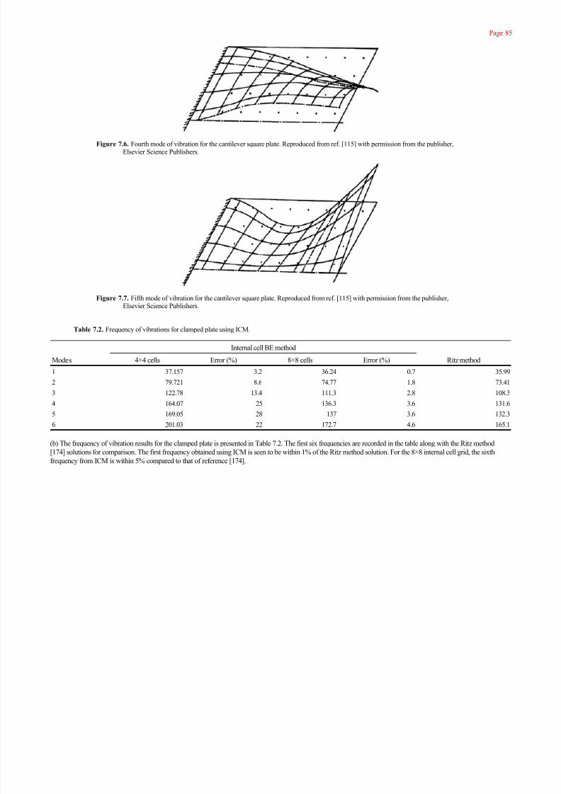
7/17/2019 The Boundary Element
http://slidepdf.com/reader/full/the-boundary-element 98/201
Page 85
Figure 7.6. Fourth mode of vibration for the cantilever square plate. Reproduced from ref. [115] with permission from the publisher,Elsevier Science Publishers.
Figure 7.7. Fifth mode of vibration for the cantilever square plate. Reproduced from ref. [115] with permission from the publisher,Elsevier Science Publishers.
(b) The frequency of vibration results for the clamped plate is presented in Table 7.2. The first six frequencies are recorded in the table along with the Ritz method
[174] solutions for comparison. The first frequency obtained using ICM is seen to be within 1% of the Ritz method solution. For the 8×8 internal cell grid, the sixth
frequency from ICM is within 5% compared to that of reference [174].
Table 7.2. Frequency of vibrations for clamped plate using ICM.
Internal cell BE method
Modes 4×4 cells Error (%) 8×8 cells Error (%) Ritz method
1 37.157 3.2 36.24 0.7 35.99
2 79.721 8.6 74.77 1.8 73.413 122.78 13.4 111.3 2.8 108.3
4 164.07 25 136.3 3.6 131.6
5 169.05 28 137 3.6 132.3
6 201.03 22 172.7 4.6 165.1

7/17/2019 The Boundary Element
http://slidepdf.com/reader/full/the-boundary-element 99/201
Page 86
(c) A closed-form analytical solution for the frequencies of vibration of a square plate with simply supported boundary conditions is available in the textbook by
Timoshenko and Woinowsky-Krieger [175]. The first five frequencies obtained using ICM are reported in Table 7.3 along the closed-form solutions. The first
frequency is within 1% of the exact solution for the 8×8 grid internal cells. The fifth frequency is about 4% apart.
Table 7.3. Frequency of vibrations for simply supported plate using ICM.
Internal cell BE method
Modes 4×4 cells Error (%) 8×8 cells Error (%) Exact solution
1 20.252 2.6 19.866 0.6 19.74
2 52.491 6.4 50.145 1.6 49.34
3 86.565 9.6 80.971 2.5 78.96
4 107.904 9.4 101.864 3.2 98.69
5 142.15 10.8 133.681 4.2 128.3

7/17/2019 The Boundary Element
http://slidepdf.com/reader/full/the-boundary-element 100/201
Page 87
Chapter 8
Algebraic Eigenvalue Problem in Boundary Elements
8.1. Introduction
In the previous chapter we used the idea of a static fundamental solution method and demonstrated its application to a mixed boundary and domain technique, whichwe designated as the Internal Cell Method (ICM). The boundary integral technique was applied to the given problem but the inertia effects were excluded in the
boundary element formulation. The domain was later divided into a grid of internal cells in order to compute the inertia term. The approach of using static fundamental
solution, free of the frequency parameter, for the dynamic problem and the separate calculation of the inertia term for computing the mass or mass-type matrix laid the
foundation for the boundary element algebraic eigenvalue formulation. However, the ICM required the discretization of the domain as well. This somewhat destroys the
advantages of the boundary element method (BEM), which is supposed to be a boundary-only method, where the discretization is confined to the boundary alone.
This chapter will present two methods, which will subject the inertia term in equations (7.9) and (7.10) to further transformation leading to boundary-only
formulation. These boundary element algebraic eigenvalue formulation methods are known as the Dual Reciprocity Method (DRM) and Particular Integral Method
(PIM). The primary motivation for these methods comes from the use of static fundamental solution as in ICM described in the previous chapter. The methods then
take the next step of removing the restriction of having to discretize the domain.
We will develop the BE algebraic eigenvalue formulation for acoustics using DRM in the following two sections. The development of BE algebraic eigenvalue
formulation for elasticity using PIM will be shown in Sections 8.4 and 8.5. The relative merits of these two methods will also be outlined.
8.2. Eigenproblem using dual reciprocity method in acoustics
As pointed out above, the idea of the development of a separate mass-type matrix in the context of BEM was first introduced in the ICM. However, this approach was
formalized by Nardini and Brebbia [116] who published the idea of separating the free vibration differential equation into two components, one, free of the frequency
parameter, leading to the stiffness-type matrix and the other, inertial term containing

7/17/2019 The Boundary Element
http://slidepdf.com/reader/full/the-boundary-element 101/201
Page 88
the frequency parameter in it, leading to the system mass matrix. The former was transformed into the boundary integral equation with the use of a fundamental solution,
independent of the frequency. On the other hand, the latter became a volume integral just like a body force term in the BEM. The dependent variable, pressure in the
volume integral (displacement components for the eigenvalue problem in elasticity), was expressed in terms of a global shape function and fictitious density function. The
volume integral was then transformed into boundary integrals with the help of Gauss’s divergence theorem. The free vibration problem could, then, be cast into a
generalized eigensystem. Nardini and Brebbia [120] later called this technique the “DRM”.
The DRM is based on the Static Green’s Function Method presented in Section 6.1.1. In the next section we shall show how the Static Green’s Function Method
extends to DRM which leads to the algebraic eigenvalue problem in BEM. Details on the choice of global shape functions that help in transforming volume integrals to
the boundary will also be shown. A number of example acoustic eigenvalue problems will be presented in Section 8.4.
8.2.1. Development of algebraic eigenvalue problem (DRM)
Here again, as in Chapter 6, we start with the acoustic Helmholtz equation. The harmonic pressure variation of a compressible fluid is governed by:
subject to the Dirichlet and/or Neumann boundary conditions:
respectively. Or, in case the fluid domain is bounded by a harmonically vibrating structure, the Neumann boundary condition takes the form:
In equations (8.1) through (8.4),
P is the amplitude of the pressure;
k is the wave number=ω/c;
ω is the circular frequency in radians/second;
c is the speed of sound through the fluid medium;
ρ is the density of the fluid, and
un
is the normal component of the displacement of the structure at fluid-structure interface.
The problem can be defined as follows: given an enclosure filled with a fluid, e.g., air, having acoustically hard (Q=∂ P /∂n=0) and partly open ( P =0) boundaries, how to
find the eigenvalues (ω) and eigenmodes (P) of the acoustic fluid within the enclosure. The case when the fluid is coupled to a harmonically vibrating structure
(boundary condition represented by equation 8.4) will be discussed in Chapter 10. In this chapter we will only deal with the most common boundary condition
represented by equation (8.3).
(8.1)
(8.2)
(8.3)
(8.4)
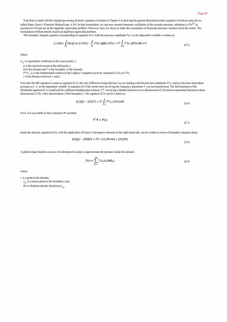
7/17/2019 The Boundary Element
http://slidepdf.com/reader/full/the-boundary-element 102/201
Page 89
Note that we dealt with the original governing dynamic equation of motion in Chapter 6 in deriving the general discretized matrix equation of motion using the so-
called Static Green’s Function Method (eqn. 6.19). In that formulation, we can now assume harmonic oscillation of the acoustic pressure, substitute p= P e jωt in
equation (6.19) and set up the algebraic eigenvalue problem. However, here we chose to make the assumption of harmonic pressure variation from the outset. The
formulation will then directly lead to an algebraic eigenvalue problem.
The boundary integral equation corresponding to equation (8.1) with the pressure amplitude P(x) as the dependent variable is written as:
where:
C P
is a geometric coefficient at the source point ξ;
n is the outward normal at the field point x;
Ω is the domain and Γ is the boundary of the domain;
P*(x, ξ) is the fundamental solution to the Laplace’s equation given by equations (2.8) or (2.9);
r is the distance between x and ξ .
Note that this BE equation is same as equation (6.3), the only difference being that here we are dealing with the pressure amplitude P(x) and not the time-dependent
pressure p(x, t) as the dependent variable. In equation (8.5) the inertia term involving the frequency parameter k was not transformed. The full treatment of the
Helmholtz equation (8.1) would call for a different fundamental solution, P*, involving a Hankel function in two-dimensional (2-D) and an exponential function in three-
dimensional (3-D). After discretization of the boundary Γ, the equation (8.5) can be written as:
Now, if it is possible to find a function Ψ such that:
inside the domain, equation (8.6), with the application of Gauss’s divergence theorem to the right-hand side, can be written in terms of boundary integrals alone:
A global shape function can now be introduced in order to approximate the pressure inside the domain:
where:
x is a point in the domain;
ξ m
is a source point at the boundary; and
Φ is a fictitious density function at ξ m
.
(8.5)
(8.6)
(8.7)
(8.8)
(8.9)

7/17/2019 The Boundary Element
http://slidepdf.com/reader/full/the-boundary-element 103/201
Page 90
The most widely used global shape function is given as:
where R is a suitable constant, e.g., the largest distance between any two points in the body. Other forms of shape functions that can be used will be discussed in next
chapter. This shape function can be inserted into equation (8.9) to express the pressure amplitude P(x) in terms of the shape functions. This pressure amplitude can then
be substituted into equation (8.7) to yield:
This differential equation can be solved for Ψ:
where:
d 1=3(d +1) and d 2=2d; d =2 and 3 for 2-D and 3-D problems, respectively. Equation (8.8) also contains the normal derivative of the function Ψ at point x, which can
be computed from equation (8.12) as:
where:
Let us now substitute the expressions of the function Ψ and its normal derivative ∂Ψ/∂n into equation (8.8) and obtain:
This equation contains both the physical pressure P and the fictitious density function Φ as the dependent variable. We can eliminate the fictitious function Φ and cast
this equation entirely in terms of pressure amplitude P and its normal derivative ∂ P /∂n. To this end, we can use the discretized boundary nodal points as the only
collocation points and write the equation (8.9) in a matrix form:
We can solve for the fictitious density function from this equation as:
Using this, equation (8.16) can be written entirely in terms of pressure amplitude and its normal derivative:
(8.10)
(8.11)
(8.12)
(8.13)
(8.14)
(8.15)
(8.16)
(8.17)
(8.18)
(8.19)

7/17/2019 The Boundary Element
http://slidepdf.com/reader/full/the-boundary-element 104/201
Page 91
Let us write this equation as:
where [M] may be recognized as the mass-type matrix, given by:
After applying appropriate boundary conditions, given in equations (8.2) and (8.3), equation (8.20) can be put in the form of generalized eigenproblem:
where:
xi are the eigenvectors [P
i , Q
i ]
k i are the eigenvalues (k
i=ω
i/c)
This method requires the inversion of a matrix [eqn. (8.18)] so as to formulate the algebraic eigenvalue problem in terms of the physical pressure. It has its advantages
since both the types of boundary conditions represented by equations (8.2) and (8.3) can easily be handled. Chapter 9 will present a modified version of DRM/PIM in
which the inversion of the matrix will be avoided [131].
8.2.2. Example problems of acoustic eigenvalue analysis (DRM)
A number of examples are presented in this section in order to demonstrate the validity and accuracy of the DRM. The boundary is discretized by linear and quadratic
elements. The boundary walls for the problems are considered acoustically hard ( Q=∂ P /∂n=0). The Lanczos eigensolver, discussed in Chapter 11, is employed to
extract the eigenvalues.
Example 8.1: Impedance tube
The impedance tube problem is suitable for validating acoustic eigenvalue solution methods. The boundary walls of the impedance tube is assumed to be acoustically
hard, ∂ P /∂n=0. The speed of sound “c” in air is taken as 340 meter/second. When the length of the tube “a” is much greater than the width “b”, i.e., for a»b and for
the lower mode shapes, the acoustic behavior of the tube may be considered as one-dimensional, for which a closed form analytical solution for the resonant frequency
in Hertz is available:
A convergence study is performed for this problem for the first five modes and the results are shown in Figure 8.1. The short side of the tube with length “b” is always
modeled with one quadratic element. The longer side with length “a” is divided into 1, 2, 4, 6, 8, 10 and 12 boundary element segments. The solutions are seen to
converge rapidly. The second mode, for example, converges to within 2% when four elements are used in the longitudinal direction. The fifth mode is seen to yield the
resonant frequency within 2% when only eight elements are used along the length of the tube.
(8.20)
(8.21)
(8.22)
(8.23)

7/17/2019 The Boundary Element
http://slidepdf.com/reader/full/the-boundary-element 105/201
Page 92
Figure 8.1. Convergence study of impedance tube resonant frequencies.
Example 8.2: Automotive passenger cabin without seats
The acoustical characteristics of the automotive passenger cabin can be conveniently investigated using a boundary element eigenvalue method such as DRM. The
computation of resonant frequencies of such passenger cabins is of importance as these cabins must be designed to have resonant frequencies away from the
frequencies of the vibrating components of the operating automobile, such as, the engine or the car stereo. In case the cabin frequency resonates with that of the
vibrating automotive components, it can cause great discomfort to the passengers.
Here we discuss the application of the BE eigenvalue method to the automotive cabin enclosure. Figure 8.2 shows a simple 2-D BE model of a small passenger car
cabin without the seats. The entire cabin is modeled using 23 quadratic boundary elements. The walls of the cabin are assumed to be acoustically hard surfaces. The
speed of sound in the enclosure air is taken as 340 meter/second. This particular problem was also solved by Shuku and Ishihara [176]. They used finite element
method (FEM) and also conducted an experimental study on the passenger compartment without the seats. The results of their studies along with the boundary element
eigensolutions are presented in Table 8.1 for the first three resonant frequencies. The finite element, boundary element and experimental solutions are seen to agree well.
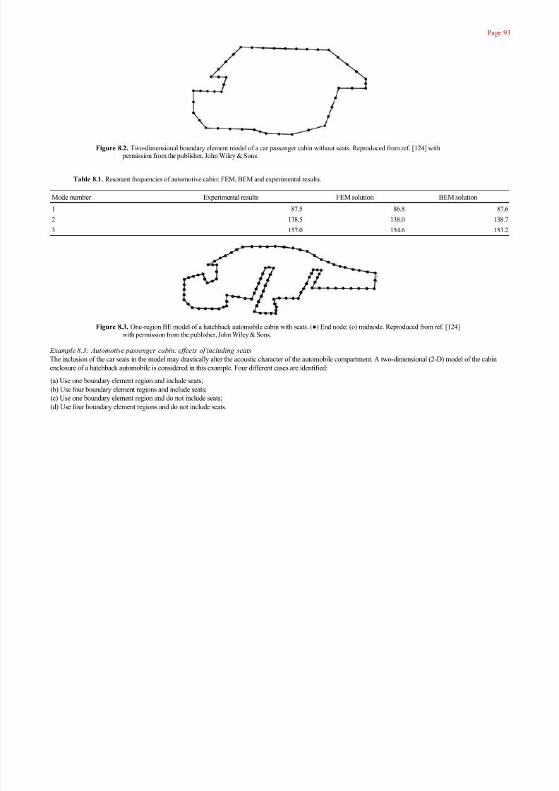
7/17/2019 The Boundary Element
http://slidepdf.com/reader/full/the-boundary-element 106/201
Page 93
Figure 8.2. Two-dimensional boundary element model of a car passenger cabin without seats. Reproduced from ref. [124] with permission from the publisher, John Wiley & Sons.
Figure 8.3. One-region BE model of a hatchback automobile cabin with seats. () End node; (o) midnode. Reproduced from ref. [124]with permission from the publisher, John Wiley & Sons.
Example 8.3: Automotive passenger cabin: effects of including seats
The inclusion of the car seats in the model may drastically alter the acoustic character of the automobile compartment. A two-dimensional (2-D) model of the cabin
enclosure of a hatchback automobile is considered in this example. Four different cases are identified:
(a) Use one boundary element region and include seats;(b) Use four boundary element regions and include seats;
(c) Use one boundary element region and do not include seats;
(d) Use four boundary element regions and do not include seats.
Table 8.1. Resonant frequencies of automotive cabin: FEM, BEM and experimental results.
Mode number Experimental results FEM solution BEM solution
1 87.5 86.8 87.6
2 138.5 138.0 138.7
3 157.0 154.6 153.2

7/17/2019 The Boundary Element
http://slidepdf.com/reader/full/the-boundary-element 107/201
Page 94
Figure 8.4. Four-region BE model of a hatchback automobile cabin with seats. () End node; (o) midnode. Reproduced from ref. [124]with permission from the publisher, John Wiley & Sons.
Figure 8.5. One-region BE model of a hatchback automobile cabin without seats. () End node; (o) midnode. Reproduced from ref.[124] with permission from the publisher, John Wiley & Sons.
Figure 8.6. Four-region BE model of a hatchback automobile cabin without seats. () End node; (o) midnode. Reproduced from ref.[124] with permission from the publisher, John Wiley & Sons.
In all cases, the walls of the automobile compartment are considered acoustically hard surfaces. The speed of sound through the air in the compartment is once again
assumed to be 340 m/s and three-noded quadratic boundary elements are used. The one-region BE model of the car with the seats included is shown in Figure 8.3,
whereas the four-region BE model with the seats is shown in Figure 8.4. Also, the one-region and four-region BE models of the car cabin without the seats are
represented in Figures 8.5 and 8.6, respectively.

7/17/2019 The Boundary Element
http://slidepdf.com/reader/full/the-boundary-element 108/201
Page 95
Figure 8.7. Three-dimensional BE model of a truck cab. Reproduced from ref. [124] with permission from the publisher, John Wiley &
Sons.
These acoustic eigenvalue problems were also studied by Nefske, Wolf and Howell [177] who analyzed the problem using 2-D FEM and compared their solutions
with experimental results. This study did not report the exact dimensions of the automobile compartment. The BE model is built from actual measurements of a
hatchback car compartment which closely resembles the model of reference [177]. The BEM, FEM and experimental results are compared against each other for all
the cases and are shown in Table 8.2. According to Nefske, Wolf and Howell, the discrepancy between their FEM and experimental solutions are due to the
contribution of the structural flexibility of the enclosing walls, i.e., in actuality, the walls were not fully acoustically hard as it was assumed in the FEM and BEM
analyses. Even though the BE analysis is performed on approximated geometric data of the cabin, the BEM solutions are seen to be remarkably close to the results
presented in reference [177].
Example 8.4: Truck cab in three dimensions
An example of a 3-D BE eigenvalue analysis is now presented. A truck cab approximately 7 ft×6 ft×5 ft 6 inches in overall dimensions was modeled using 55 eight-
noded quadratic serendipity quadrilateral boundary elements and two six-noded quadratic triangular boundary elements (Fig. 8.7). The total number of boundary
element nodes for this discretization turns out to be 171. The boundary walls once again are considered as acoustically hard surfaces and the speed of sound is taken as
340 m/s. This problem was also investigated by Nefske, Wolf and Howell [177] in which they used 3-D finite elements. Here also they did not report any dimension of
the truck cab. The above dimensions closely resembled the model used in reference [177] and
Table 8.2. Resonant frequencies of a hatchback automotive cabin: FEM, BEM and experimental results.
Without seats With seats
BEM BEM
Mode Experiment FEM Mesh 1 Mesh 2 Experiment FEM Mesh 1 Mesh 2
1 60 68 69 72 53 50 49 49
2 110 105 104 110 — 79 75 78
3 135 152 153 155 — 125 116 122
4 — 179 190 186 — 163 193 159
Mesh 1: One-region BE mesh.
Mesh 2: Four-region BE mesh.
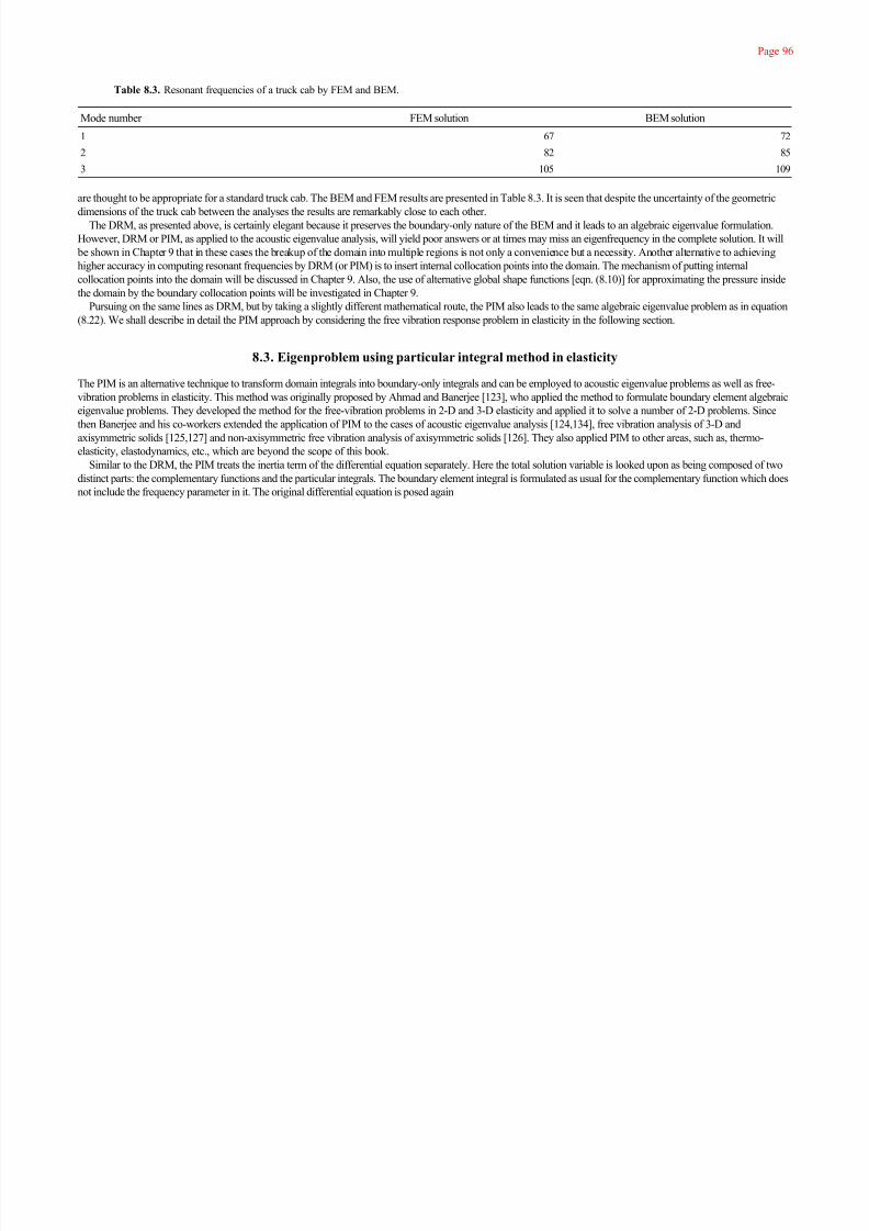
7/17/2019 The Boundary Element
http://slidepdf.com/reader/full/the-boundary-element 109/201
Page 96
are thought to be appropriate for a standard truck cab. The BEM and FEM results are presented in Table 8.3. It is seen that despite the uncertainty of the geometricdimensions of the truck cab between the analyses the results are remarkably close to each other.
The DRM, as presented above, is certainly elegant because it preserves the boundary-only nature of the BEM and it leads to an algebraic eigenvalue formulation.
However, DRM or PIM, as applied to the acoustic eigenvalue analysis, will yield poor answers or at times may miss an eigenfrequency in the complete solution. It will
be shown in Chapter 9 that in these cases the breakup of the domain into multiple regions is not only a convenience but a necessity. Another alternative to achieving
higher accuracy in computing resonant frequencies by DRM (or PIM) is to insert internal collocation points into the domain. The mechanism of putting internal
collocation points into the domain will be discussed in Chapter 9. Also, the use of alternative global shape functions [eqn. (8.10)] for approximating the pressure inside
the domain by the boundary collocation points will be investigated in Chapter 9.
Pursuing on the same lines as DRM, but by taking a slightly different mathematical route, the PIM also leads to the same algebraic eigenvalue problem as in equation
(8.22). We shall describe in detail the PIM approach by considering the free vibration response problem in elasticity in the following section.
8.3. Eigenproblem using particular integral method in elasticity
The PIM is an alternative technique to transform domain integrals into boundary-only integrals and can be employed to acoustic eigenvalue problems as well as free-
vibration problems in elasticity. This method was originally proposed by Ahmad and Banerjee [123], who applied the method to formulate boundary element algebraiceigenvalue problems. They developed the method for the free-vibration problems in 2-D and 3-D elasticity and applied it to solve a number of 2-D problems. Since
then Banerjee and his co-workers extended the application of PIM to the cases of acoustic eigenvalue analysis [124,134], free vibration analysis of 3-D and
axisymmetric solids [125,127] and non-axisymmetric free vibration analysis of axisymmetric solids [126]. They also applied PIM to other areas, such as, thermo-
elasticity, elastodynamics, etc., which are beyond the scope of this book.
Similar to the DRM, the PIM treats the inertia term of the differential equation separately. Here the total solution variable is looked upon as being composed of two
distinct parts: the complementary functions and the particular integrals. The boundary element integral is formulated as usual for the complementary function which does
not include the frequency parameter in it. The original differential equation is posed again
Table 8.3. Resonant frequencies of a truck cab by FEM and BEM.
Mode number FEM solution BEM solution
1 67 72
2 82 85
3 105 109

7/17/2019 The Boundary Element
http://slidepdf.com/reader/full/the-boundary-element 110/201
Page 97
with the particular integral part of the solution, treating the inertia term as the forcing function. As in the DRM, the total solution variable appearing in the inertia term is
approximated using global shape functions and the particular integral is solved for. The complementary function and the particular integral are added together to obtain
the final solution. In the process, a distinct mass-type matrix is formed which puts the frequency parameter outside the matrix as a multiplier.
As applied to structural free-vibration problems, PIM (and DRM) will produce vibration frequency solutions that are dependent on the level of discretization of the
boundary only and will not require internal collocation points for improving solution accuracy. However, when PIM is applied to acoustic algebraic eigenvalue analysis
[124], the global shape function used to approximate the total pressure in the inertia term is not adequate to yield accurate solutions for many situations. In these cases,
it will be necessary to insert internal collocation points to obtain more accurate resonant frequencies.
We will present the detailed description of the PIM, as applied to free-vibration problems, in the following section. We will develop formulations for 2-D and 3-D
cases.
8.3.1. Development of algebraic eigenvalue problem (PIM)
The time-harmonic governing differential equation of an elastic, homogeneous and isotropic body can be written as:
This is the elastodynamic equilibrium equation for harmonic vibration written in terms of displacements in the absence of body forces. In the above equation, μ is the
shear modulus (eqn. 6.21), λ is the Lamé’s constant and ρ is the density. For convenience, this equation will be written in terms of a differential operator L, which can
be defined as:
As a result, equation (8.24) can be written in a compact form:
In PIM, the total displacement solutions ui and the tractions t
i on the boundary are divided into complementary functions and particular solutions in the following
manner:
The complementary function, , satisfies the first term of equation (8.26):
The particular solution, , on the other hand, satisfies the following equation:
Note that the second term of equation (8.30) contains the total displacement solution, ui , in the domain which will be approximated using a set of global shape
functions. We will come back to this later in this section. First, we write the boundary integral
(8.24)
(8.25)
(8.26)
(8.27)
(8.28)
(8.29)
(8.30)

7/17/2019 The Boundary Element
http://slidepdf.com/reader/full/the-boundary-element 111/201
Page 98
equation for the complementary function, , in equation (8.29) using the static Green’s function:
where are the Kelvin’s displacement and traction fundamental solutions, respectively, given by the equations (6.23) through (6.26). After discretization of the
boundary Γ this boundary integral equation can be transformed into matrix BE equation:
We can now substitute the total displacements and tractions for the complementary functions uc and t c appearing in this equation using equations (8.27) and (8.28),
leading to:
The particular solution u p , appearing here, must be solved from the differential equation (8.30). To this end, total displacement solution ui inside the domain Ω, which
appears in the second term of equation (8.30), will be approximated, as it was done in the case of DRM, using an unknown fictitious density function Φ and a known
global shape function just as we did in equation (6.29):
This step is same as in equation (8.9) except for the global shape function notation, which is here in place of C .
Given a specific form of the known functions , equation (8.30) can be solved for the particular solution, u p , and then the traction components, t p, can be computed.
It may be noted here that we are essentially approximating the inertia term of the differential equation in an attempt to compute the mass matrix. The computation of this
term does not involve any spatial differentiation and as such it suffices most often to approximate this term with simpler functions compared to the stiffness terms. As
done in the DRM, we will assume a set of global shape functions for these known functions :
where R can be taken as the largest distance between two points on the body and r is the distance between the field point x and the source point ξ m
. Upon substitution
of the approximation (8.34) for the domain displacement, ui , the particular integral differential equation (8.30) becomes:
The particular solution, u p , can now be chosen in such a way that it satisfies this equation. It can be written in the following manner:
(8.31)
(8.32)
(8.33)
(8.34)
(8.35)
(8.36)
(8.37)

7/17/2019 The Boundary Element
http://slidepdf.com/reader/full/the-boundary-element 112/201
Page 99
The displacement function, D, which satisfies equation (8.36) is found to be:
where:
d =2 for 2-D problems and 3 for 3-D problems. For 2-D problems, for example, D is given by:
The traction components, , are found to be:
The traction functions are given by:
where:
Thus, for 2-D problems, T would take the following form:
(8.38)
(8.39)
(8.40)
(8.41)
(8.42)
(8.43)
(8.44)
(8.45)
(8.46)
(8.47)
(8.48)
(8.49)

7/17/2019 The Boundary Element
http://slidepdf.com/reader/full/the-boundary-element 113/201
Page 100
We can obviously use the nodes on the boundary as the collocation points for the evaluation of the displacement and traction functions D and T respectively and write
the equations (8.37) and (8.44) in the matrix form:
Substituting these discretized particular solutions of displacements and tractions back into equation (8.33) we arrive at the following:
Combining equations (8.34) and (8.35) we can write the total displacement approximation in terms of known functions and fictitious functions:
This relationship between the total displacement and fictitious function can be written in matrix form using the discretized boundary points as the collocation points:
We can solve for Φ from this relationship by inverting the matrix [C]:
After substituting this value of Φ into equation (8.52), we can express the equilibrium equation entirely in terms of physical variables, such as, displacement and
traction:
This can be written as:
where [M] is the desired mass matrix:
After applying appropriate displacement and traction boundary conditions, ui=0 and t
i=0 respectively, we can cast equation (8.57) into a generalized eigenvalue
problem:
where:
xi are the eigenvectors [u
i , t
i ]
k i are the eigenvalues (k
i=ω
i/c)
The natural frequencies of vibration of 2-D and 3-D elastic bodies can be computed by solving this generalized eigenvalue problem. Note that eigenvalue formulation
for axisymmetric elastic bodies will require a separate formulation because a different fundamental solution will have to be used. The next section will present a number
of 2-D and 3-D free vibration analysis examples in elasticity.
(8.50)
(8.51)
(8.52)
(8.53)
(8.54)
(8.55)
(8.56)
(8.57)
(8.58)
(8.59)

7/17/2019 The Boundary Element
http://slidepdf.com/reader/full/the-boundary-element 114/201
Page 101
8.3.2. Example problems of eigenvalue analysis in elasticity
Unlike the finite element formulation, the system stiffness and mass matrices [A ] and [B] respectively, resulting from boundary element formulation, are fully
populated and unsymmetric. As a result, special eigenvalue extraction routines will be needed to compute frequencies and mode shapes from unsymmetric mass and
stiffness matrices. Rajakumar and Rogers [178] and Rajakumar [179] developed the Lanczos algorithm, which is applied to unsymmetric generalized eigenvalue
problems. This algorithm has been successfully applied to fully populated and unsymmetric mass and stiffness matrices generated by the BEM [131,132,136,137].
Ahmad and Banerjee [123] used the eigenvalue extraction algorithm developed by Moller and Stewart [180] to solve for the frequencies of vibration of elastic bodies.
Example 8.5: Two-dimensional square and triangular elastic bodies
The triangular cantilevered planar elastic body is 10 units at the supported base with a span of eight units (Fig. 8.8). The material properties are taken as E / ρ=10,000and v=0.2 ( E =Young’s Modulus, ρ=density and v=Poisson’s ratio). Different levels of boundary element discretizations are used to study the convergence behavior of
the boundary element formulation. The results for first four modes are shown in Table 8.4. The time periods for the four modes from finite element runs with
corresponding number of boundary nodes are found to be 0.430, 0.212, 0.192 and 0.125, respectively.
Figure 8.8. Convergence studies of time periods of planar square and triangular elastic bodies (FEM model with 121 nodes).

7/17/2019 The Boundary Element
http://slidepdf.com/reader/full/the-boundary-element 115/201
Page 102
The square cantilevered planar elastic body is 6 units×6 units (Fig. 8.8). The material properties are once again taken as E/ρ=10,000 and v=0.2. Here also different
levels of boundary element discretizations are used to study convergence. The results for first four modes are shown in Table 8.5. The time periods from finite element
runs are found to be 0.585, 0.238, 0.187 and 0.126, respectively. In both cases the boundary element solutions are seen to converge to the correct results for a small
number of elements.
Example 8.6: Cantilever beam
The free vibration analysis is performed on a deep cantilevered beam of length= 24 units and height=6 units (Fig. 8.9). The material properties are E/ρ=10,000 and
v=0.2. A number of boundary element discretizations are used and the results are compared with finite element solutions. The first, second and fourth modes represent
transverse vibration, whereas the third and fifth modes represent longitudinal vibration. The boundary element results compare very well with those of the finite element
for the longitudinal modes. In order to obtain the same level of accuracy for the transverse modes, more boundary elements will be needed in the transverse direction.
In general, the boundary element results are seen to compare well with those of finite elements.
Example 8.7: Shear wall
Next a shear wall with four openings is selected for study. The wall is modeled by BEM as well as FEM. The two discretizations are shown in Figure 8.10. The
boundary element mesh consists of 29 quadratic line elements with 58 nodes, whereas the finite element mesh consists of 476 two-dimensional four-noded planar solid
finite elements
Table 8.4. Time periods of free vibration of triangular cantilevered elastic body.
Number of elements Model Mode 2 Mode 3 Mode 4
3 0.432 0.207 0.138 0.081
6 0.430 0.212 0.180 0.095
9 0.430 0.212 0.189 0.104
12 0.430 0.212 0.191 0.109
15 0.430 0.212 0.192 0.111
18 0.430 0.212 0.192 0.112
Table 8.5. Time periods of free vibration of square cantilevered elastic body.
Number of elements Model Mode 2 Mode 3 Mode 4
4 0.561 0.235 0.172 0.107
6 0.568 0.237 0.179 0.116
8 0.581 0.238 0.185 0.122
10 0.581 0.238 0.187 0.123
12 0.584 0.238 0.187 0.125
16 0.585 0.238 0.187 0.125
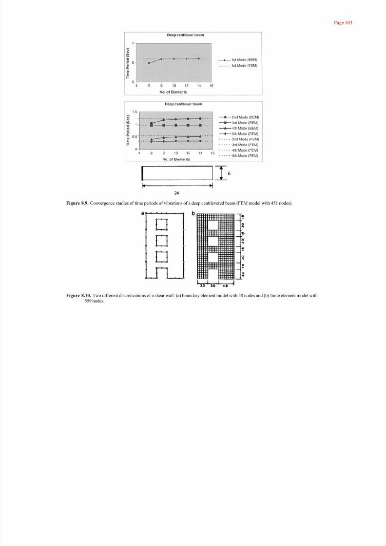
7/17/2019 The Boundary Element
http://slidepdf.com/reader/full/the-boundary-element 116/201
Page 103
Figure 8.9. Convergence studies of time periods of vibrations of a deep cantilevered beam (FEM model with 451 nodes).
Figure 8.10. Two different discretizations of a shear wall: (a) boundary element model with 58 nodes and (b) finite element model with559 nodes.
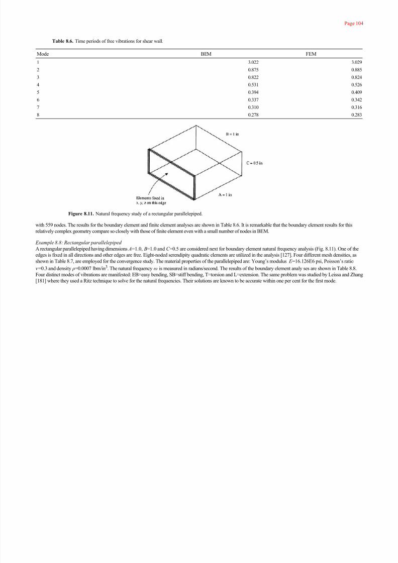
7/17/2019 The Boundary Element
http://slidepdf.com/reader/full/the-boundary-element 117/201
Page 104
Figure 8.11. Natural frequency study of a rectangular parallelepiped.
with 559 nodes. The results for the boundary element and finite element analyses are shown in Table 8.6. It is remarkable that the boundary element results for this
relatively complex geometry compare so closely with those of finite element even with a small number of nodes in BEM.
Example 8.8: Rectangular parallelepiped
A rectangular parallelepiped having dimensions A=1.0, B=1.0 and C =0.5 are considered next for boundary element natural frequency analysis (Fig. 8.11). One of the
edges is fixed in all directions and other edges are free. Eight-noded serendipity quadratic elements are utilized in the analysis [127]. Four different mesh densities, as
shown in Table 8.7, are employed for the convergence study. The material properties of the parallelepiped are: Young’s modulus E =16.126E6 psi, Poisson’s ratio
v=0.3 and density ρ=0.0007 lbm/in3. The natural frequency ω is measured in radians/second. The results of the boundary element analy ses are shown in Table 8.8.
Four distinct modes of vibrations are manifested: EB=easy bending, SB=stiff bending, T=torsion and L=extension. The same problem was studied by Leissa and Zhang[181] where they used a Ritz technique to solve for the natural frequencies. Their solutions are known to be accurate within one per cent for the first mode.
Table 8.6. Time periods of free vibrations for shear wall.
Mode BEM FEM
1 3.022 3.029
2 0.875 0.885
3 0.822 0.824
4 0.531 0.526
5 0.394 0.409
6 0.337 0.342
7 0.310 0.316
8 0.278 0.283

7/17/2019 The Boundary Element
http://slidepdf.com/reader/full/the-boundary-element 118/201
Page 105
The boundary element analysis results in terms of the frequency parameter are listed in Table 8.8 where these are compared against those of the Ritz
method. The first mode for each displacement type is seen to converge rapidly. More boundary elements will be needed in the longitudinal (side B) direction in order to
achieve higher rate of convergence for the higher modes.
Example 8.9: Automobile crankshaft
In this example, a half symmetry model of an automobile crankshaft is considered [127]. It is modeled by eight-noded serendipity quadratic boundary elements as
shown in Figure 8.12. The wider end was held by rigid lubricated rollers along outer edges and the rest of the surface was left free. The crankshaft was also modeled
by finite elements in which the surface discretization was taken to be the same as the boundary element mesh. The results of the frequency analysis are presented in
Table 8.9. The first, second and fourth mode frequencies are seen to be in good agreement.Wilson, Miller and Banerjee [127] reports that the finite element solution failed to yield the third natural frequency for the given level of discretization. When the finite
element mesh was refined, it yielded the third frequency as 47,600 Hz, leaving the first, second and fourth frequency essentially unchanged.
It can be pointed out here that there is a subtle but important distinction between the free vibration problem in elasticity and that in acoustics. The mode shapes in the
elasticity free vibration problem are somewhat controlled by the problem boundary,
Table 8.7. Different boundary element discretizations used for the rectangular parallelepiped.
Elements along side…
Model A B C Number of elements Number of nodes
1 1 1 1 6 20
2 1 2 1 10 32
3 1 3 1 14 44
4 2 3 1 22 68
Table 8.8. Convergence study of natural frequencies of a rectangular parallelepiped.
Mode Type Ritz Mesh 1 (%) Mesh 2 (%) Mesh 3 (%) Mesh 4 (%)
1 EB 0.447 0.472 5.5 0.429 −4.0 0.435 −2.7 0.442 −1.2
2 SB 0.667 0.664 −0.4 0.666 −0.3 0.668 0.1 0.661 −0.8
3 T 0.788 0.887 12.5 0.829 5.1 0.820 4.0 0.788 0.0
4 L 1.596 1.625 1.8 1.620 1.5 1.618 1.4 1.602 0.4
5 EB 1.664 2.136 28.3 1.797 8.0 1.729 3.9 1.689 1.5
6 SB 1.774 1.836 3.5 1.789 0.9 1.775 0.1
7 T 2.220 2.552 14.9 2.448 10.3 2.285 2.9
8 EB 2.278 3.033 33.3 2.365 3.8
9 L 2.797 2.842 1.6
10 SB 3.068 3.249 5.9
Mode type identification: EB=easy bending, SB=stiff bending, T=torsion and L=extension.

7/17/2019 The Boundary Element
http://slidepdf.com/reader/full/the-boundary-element 119/201
Page 106
Figure 8.12. Boundary element mesh of automobile crankshaft.
the domain being in tune with the boundary because of compatibility conditions. On the contrary, in the case of acoustics, the problem boundary does influence
eigenmodes, but it does not control them to the same extent as in the elasticity problem. Rather eigenmodes are governed here by the continuity of the eigenfunctions.
As a result, compared to elasticity problems, more internal collocation points will be required to accurately solve truly 2-D or 3-D acoustic eigenvalue problems having
complex eigenfunctions. The method of introducing internal collocation points in the domain will be developed in Chapter 9.
Table 8.9. Natural frequencies (Hz) of automobile crankshaft.
Mode Finite element solution Boundary element solution
1 17,400 18,200
2 35,800 34,300
3 — 47,500
4 66,300 66,300
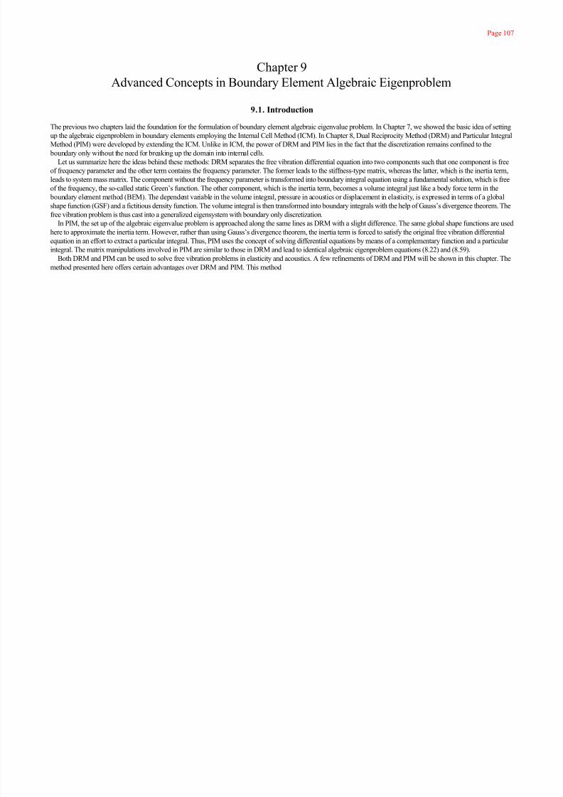
7/17/2019 The Boundary Element
http://slidepdf.com/reader/full/the-boundary-element 120/201
Page 107
Chapter 9
Advanced Concepts in Boundary Element Algebraic Eigenproblem
9.1. Introduction
The previous two chapters laid the foundation for the formulation of boundary element algebraic eigenvalue problem. In Chapter 7, we showed the basic idea of settingup the algebraic eigenproblem in boundary elements employing the Internal Cell Method (ICM). In Chapter 8, Dual Reciprocity Method (DRM) and Particular Integral
Method (PIM) were developed by extending the ICM. Unlike in ICM, the power of DRM and PIM lies in the fact that the discretization remains confined to the
boundary only without the need for breaking up the domain into internal cells.
Let us summarize here the ideas behind these methods: DRM separates the free vibration differential equation into two components such that one component is free
of frequency parameter and the other term contains the frequency parameter. The former leads to the stiffness-type matrix, whereas the latter, which is the inertia term,
leads to system mass matrix. The component without the frequency parameter is transformed into boundary integral equation using a fundamental solution, which is free
of the frequency, the so-called static Green’s function. The other component, which is the inertia term, becomes a volume integral just like a body force term in the
boundary element method (BEM). The dependent variable in the volume integral, pressure in acoustics or displacement in elasticity, is expressed in terms of a global
shape function (GSF) and a fictitious density function. The volume integral is then transformed into boundary integrals with the help of Gauss’s divergence theorem. The
free vibration problem is thus cast into a generalized eigensystem with boundary only discretization.
In PIM, the set up of the algebraic eigenvalue problem is approached along the same lines as DRM with a slight difference. The same global shape functions are used
here to approximate the inertia term. However, rather than using Gauss’s divergence theorem, the inertia term is forced to satisfy the original free vibration differential
equation in an effort to extract a particular integral. Thus, PIM uses the concept of solving differential equations by means of a complementary function and a particular
integral. The matrix manipulations involved in PIM are similar to those in DRM and lead to identical algebraic eigenproblem equations (8.22) and (8.59).
Both DRM and PIM can be used to solve free vibration problems in elasticity and acoustics. A few refinements of DRM and PIM will be shown in this chapter. Themethod presented here offers certain advantages over DRM and PIM. This method

7/17/2019 The Boundary Element
http://slidepdf.com/reader/full/the-boundary-element 121/201
Page 108
may be designated as “Fictitious Function Method” (FFM). It is primarily based on DRM and PIM. The idea behind this method is to temporarily retain the fictitious
density function Φ in equations (8.16) and (8.52) as the system variable instead of the original dependent variable, pressure (P in acoustics or displacement u in
elasticity.
Note that the relationship between the original dependent variable and the fictitious function [eqns. (8.17) and (8.54)] represents a linear transformation. The
eigenvalues of the system remain unchanged under this change of variables. The eigenvectors in terms of the original variable can be retrieved very easily through
equations (8.17) and (8.54). As a result of the use of the fictitious density function rather than the original dependent variable as the system variable, we can avoid the
matrix inversion shown in equations (8.18) and (8.55).
FFM is particularly helpful for the commonly encountered pure Neumann problem (Q=∂ P /∂n=0) in acoustics. However, it is also applicable to problem where a
part of the boundary is of the Dirichlet type ( P =0 or u=0). In this case, a small size matrix needs to be inverted. The same observation would remain true for the fluid-
structure coupled problems in which the boundary conditions on the wall are given by Q=∂ P /∂n= ρω2U n. The eigenvalue formulation details for the fluid-structure
coupled problem will be presented in Chapter 10.
9.2. Algebraic eigenvalue formulation using fictitious function method
This method utilizes the property of matrices that the eigenvalues of a matrix remain the same under a linear transformation of its eigenvectors. The eigenfrequencies are
extracted along with the transformed eigenvectors. Because the inversion of a matrix of size as large as the system matrix is avoided, FFM is computationally more
efficient for large problems with Neumann boundary conditions. Details of FFM are presented below, followed by an example problem.
We develop the FFM here starting with the PIM presented in Chapter 8. The problem of acoustic eigenanalysis was posed in equations (8.1) through (8.4). In the
PIM we saw that the total pressure is split into two components, a complementary function pressure and a particular solution pressure:
The complementary function pressure satisfies the Laplacian portion of the governing equation:
and the particular solution pressure will satisfy
The boundary integral statement of equation (9.2) is set up using the static Green’s function (frequency-independent fundamental solution) approach as given in
equations (2.8) and (2.9). Here we rewrite the resulting Boundary Element matrix equation for complimentary function pressure:
(9.1)
(9.2)
(9.3)
(9.4)

7/17/2019 The Boundary Element
http://slidepdf.com/reader/full/the-boundary-element 122/201
Page 109
The complementary function pressure is eliminated from this equation using the relationships given in equations (9.1):
The particular integrals P I must be obtained by solving equation (9.3). To this end, the pressure P inside the domain is approximated using a GSF and fictitious density
functions, shown in equations (8.9) and (8.10). Substituting for the total pressure from equation (8.9) into equation (9.3), we obtain:
The particular integral pressure, P I , can be solved from this equation employing one of the differential equation solution methods, such as, either a trial and error method
or the method of undetermined coefficients. The following particular integral solution satisfies the above equation and, therefore, is a solution to this equation:
The normal gradient QI=∂ P I/∂n for the particular integral P I can now be computed. Let us write the particular integral solutions in matrix form:
Substituting these into equation (9.5), we obtain the algebraic eigenvalue problem in terms of both the pressure P and the fictitious density function Φ:
This is rewritten as:
with this definition of mass-type matrix:
In standard DRM or PIM, the fictitious density functions Φ are eliminated in favor of the physical pressures P using the relation given in equation (8.17). See
Chapter 8 for further details on standard DRM and PIM.
For acoustic eigenvalue analysis in particular, most frequently the task is to compute resonant frequencies of closed cavities with acoustically rigid boundaries. In this
case, it can be seen from equations (9.10) and (8.17) that, if the eigenvalue problem is posed in terms of Φ rather than P, the inversion of the [C] matrix can be
avoided, leaving the eigenvalues unchanged. Here we work with a set of fictitious density functions Φ only temporarily, as the eigenmodes in terms of P can be
easily retrieved using equation (8.17). Detailed derivations of FFM for different boundary conditions are given below.
(9.5)
(9.6)
(9.7)
(9.8)
(9.9)
(9.10)
(9.11)

7/17/2019 The Boundary Element
http://slidepdf.com/reader/full/the-boundary-element 123/201
Page 110
9.2.1. Fictitious function method with pure Neumann boundary condition
Consider the case in which all the boundary walls of the enclosure are acoustically hard, i.e., Q=∂ P /∂n=0 for all nodes on the boundary. Then equation (9.9) becomes:
Substituting the values of P from equation (8.17) into the above, the entire formulation can be posed in terms of the fictitious density functions Φ:
Let us rewrite this equation in compact form:
with the following definition of stiffness-type matrix:
The eigenvalues λ=k 2 of this eigensystem is the same as that of equation (8.19). The only difference is that equation (9.14) does not require any matrix inversion. Theeigenvectors in terms of physical variable P can be obtained from equation (8.17), if desired.
9.2.2. Fictitious function method with mixed boundary conditions
In case the boundary conditions on the walls of the enclosures are mixed with both Neumann and Dirichlet type conditions:
equations (9.10) and (8.17) can be partitioned as:
n1
+n2
=n, total number of nodes on the boundary. The above partitioned equations can be turned into:
Equations (9.19) and (9.20) can be used to extract eigenvalues and eigenvectors for mixed boundary conditions. We note here that FFM would not be efficient for
large values of n2
.
9.2.3. Fictitious function method in fluid-structure interaction problem
Fictitious Function Method can also be applied to the eigenvalue analysis of coupled fluid-structure problems. The Neumann boundary condition takes the form given in
equation (8.4), ∂ P /∂n= ρω2un , when the acoustic fluid is in contact with a vibrating
(9.12)
(9.13)
(9.14)
(9.15)
(9.16)
(9.17)
(9.18)
(9.19)
(9.20)

7/17/2019 The Boundary Element
http://slidepdf.com/reader/full/the-boundary-element 124/201
Page 111
structure. Using this fluid-structure boundary condition in equation (9.10) one can write:
This can be rewritten in the following form:
where:
n x
and ny respectively, are the x and y components of the unit normal at the interface boundary and u are the structural displacements. The matrix equation for the
vibrating structure can be written down, accounting for the fluid pressure load at the fluid-structure interface, as follows:
With the help of equation (8.17), equation (9.24) can be written as:
where [ K s
] and [Ms
] are the structural stiffness and mass matrices, respectively. [R] is the coupling matrix representing the surface area on which the fluid pressure
load acts on the structure at the fluid-structure interface. Equations (9.22) and (9.25) can be combined together in the form:
This equation can be used to study an interesting class of eigenvalue problems involving acoustic fluid-structure interaction. This subject will be further studied in details
in Chapter 10 where example problems for fluid-structure interaction will be discussed.
9.3. Example problems using fictitious function method
Example 9.1: Impedance tube
The impedance tube problem was considered in Chapter 8 in the context of standard DRM. Here the same problem is used to illustrate FFM. Acoustics laboratories
commonly use this set-up for experimental purposes (Fig. 9.1). The boundary walls of the impedance tube are assumed to be acoustically hard with ∂ P/ ∂n=0. The
speed of sound “c” in the air is taken as 340 m/s. The tube length and width are chosen to be a=40 m and b=2 m, respectively. Sixteen linear elements are used along
the length and two elements along the width of the tube.
The results of the analysis are shown in Table 9.1 where the theoretical solutions are also shown for comparison. The results from FFM are seen to be in good
agreement with the theoretical solutions. The eigenmodes are presented in Figure 9.2 in terms of physical pressures as well as fictitious function Φ. For this one-
dimensional problem,
(9.21)
(9.22)
(9.23)
(9.24)
(9.25)
(9.26)

7/17/2019 The Boundary Element
http://slidepdf.com/reader/full/the-boundary-element 125/201
Page 112
Figure 9.1. Impedance tube (speed of sound c=340 m/s).
the variation of Φ is seen to closely follow that of P . The fifth mode containing two full sine waves is marginally captured here with only four linear segments per half sine
wave.
9.4. Effect of internal collocation points on eigensolutions
It was pointed out earlier that unlike in BE elastic eigenvalue analysis, the BE acoustic eigenvalue analysis will require internal collocation points for accurate solutions.
The global shape functions, given by equation (8.10), used to approximate the total pressure in DRM as well as PIM are not adequate in representing true two-
dimensional (2-D) or three-dimensional (3-D) eigenmodes. In order to prove the need for internal collocation points for eigenfrequency computation, let us consider the
extreme case of a circular acoustic enclosure (Fig. 9.3) with Neumann boundary conditions, ∂ P /∂n=0, on the boundary wall. Theoretical eigenfrequency solutions for
this circular domain Neumann problem are given by the characteristic equation:
( ) is the first derivative of the m-th order Bessel’s function of the first kind. The circular boundary is discretized first using 36 linear segments. The boundary is next
discretized using quadratic elements with the same number of nodal points. The results are presented in Table 9.2, where the theoretical solutions as well as solutions
from ANSYS [160] acoustic finite element run are also presented. It can be seen that the quadratic representation of the boundary improves the solution slightly, butthey are still poor. It means that no matter how good the boundary discretization, the boundary element acoustic eigenvalue analysis without internal points will yield
very poor results in this case, even for the fundamental mode. Furthermore, it fails to yield the ring mode solution. It happens because all the modes for the circular
domain are truly 2-D, which
Table 9.1. Comparison of eigenvalues for impedance tube.
Mode FFM (Hz) Theory (Hz)
1 0 0
2 4.26 4.25
3 8.53 8.50
4 12.91 12.75
5 17.30 17.0
(9.27)

7/17/2019 The Boundary Element
http://slidepdf.com/reader/full/the-boundary-element 126/201
Page 113
Figure 9.2. Eigenmodes of the impedance tube.
means that the shape of eigenfunctions can have dramatic variations within the domain and boundary nodes alone are not capable of describing the modes adequately.
This observation is obviously true for DRM, PIM and FFM.
Here we will show how to insert internal collocation points in the domain [116,131] and how to include these internal domain pressure variables as part of the total

7/17/2019 The Boundary Element
http://slidepdf.com/reader/full/the-boundary-element 127/201
Page 114
Figure 9.3. Circular acoustic enclosure (speed of sound c=340 m/s).
problem. Note that the eigensolutions can also be improved by dividing the domain into several regions. See Chapter 4 for zoning procedure in BEM.
In Chapter 2 we showed that after the solution of potential and its normal derivatives on the boundary collocation points, the solution inside the domain can be found
using equations (2.28) and (2.29). In the present case, the pressure inside the domain can be computed using the pressure P and pressure gradients q on the
boundary:
[I] is an identity matrix of order which equals to the number of internal points used. These internal point solutions can be combined with the boundary solutions given inequation (9.13) to yield:
where:
] are the augmented matrices containing the
Table 9.2. Eigenvalues of circular domain without internal points.
DRM/PIM/FFM
Mode Linear elements (Hz) Quadratic elements (Hz) Finite element (216 elements) (Hz) Theory (Hz)
1 105.15 104.89 100.02 99.63
2 105.15 104.89 100.02 99.63
3 177.10 176.12 166.33 165.27
4 177.10 176.12 166.33 165.275 — — 209.40 207.34
6 247.44 246.09 229.88 227.34
7 247.44 246.09 229.88 227.34
(9.28)
(9.29)
(9.30)

7/17/2019 The Boundary Element
http://slidepdf.com/reader/full/the-boundary-element 128/201
Page 115
coefficients of internal points as well as the boundary nodes corresponding to [C], [D] and [T ] matrices, respectively. Equation (9.29) will yield more accurate
eigensolutions because of the representation of eigenfunctions on the boundary as well as inside the domain. The next section will present example problems to
demonstrate the effects of inclusion of internal collocation points in the problem.
9.4.1. Examples to show effect of internal collocation points on eigensolutions
Example 9.2: Circular acoustic domain with internal points
Let us consider the same circular domain problem. This time it is solved using varying number of internal collocation points. The results are presented in Table 9.3 for
linear elements and Table 9.4 for quadratic elements. It can be seen that the results improve considerably with the gradual addition of internal node points. The ring
mode solution appears with the addition of only one internal point at the center of the domain.
Example 9.3: Trapezoidal acoustic domain A trapezoidal acoustic domain is considered next (Fig. 9.4). Finite element solutions as well as experimental results for this problem are reported by Shuku and Ishihara
[176]. This problem is solved using FFM without and with internal points. The results are presented in Table 9.5 where the finite element and experimental solutions are
also included for comparison. In this case, the first mode is essentially one-dimensional and the solution appears to be reasonable for this mode without the use of
internal
Table 9.3. Eigenvalues of circular domain with and without internal points (linear elements).
Mode No internal points (Hz) One internal point (Hz) Five internal points (Hz) Nine internal points (Hz)
1 105.15 105.15 102.42 101.50
2 105.15 105.15 102.42 101.50
3 177.10 177.10 172.23 172.23
4 177.10 177.10 177.10 172.23
5 — 239.12 225.76 221.97
6 247.44 247.44 246.05 243.66
7 247.44 247.44 246.05 243.66
Table 9.4. Eigenvalues of circular domain with and without internal points (quadratic elements).
Mode No internal points (Hz) One internal point (Hz) Five internal points (Hz) Nine internal points (Hz)
1 104.89 104.89 102.19 101.27
2 104.89 104.89 102.19 101.27
3 176.12 176.12 171.45 171.45
4 176.12 176.12 176.12 171.45
5 — 239.22 225.76 221.97
6 246.09 246.09 244.75 242.42
7 246.09 246.09 244.75 242.42
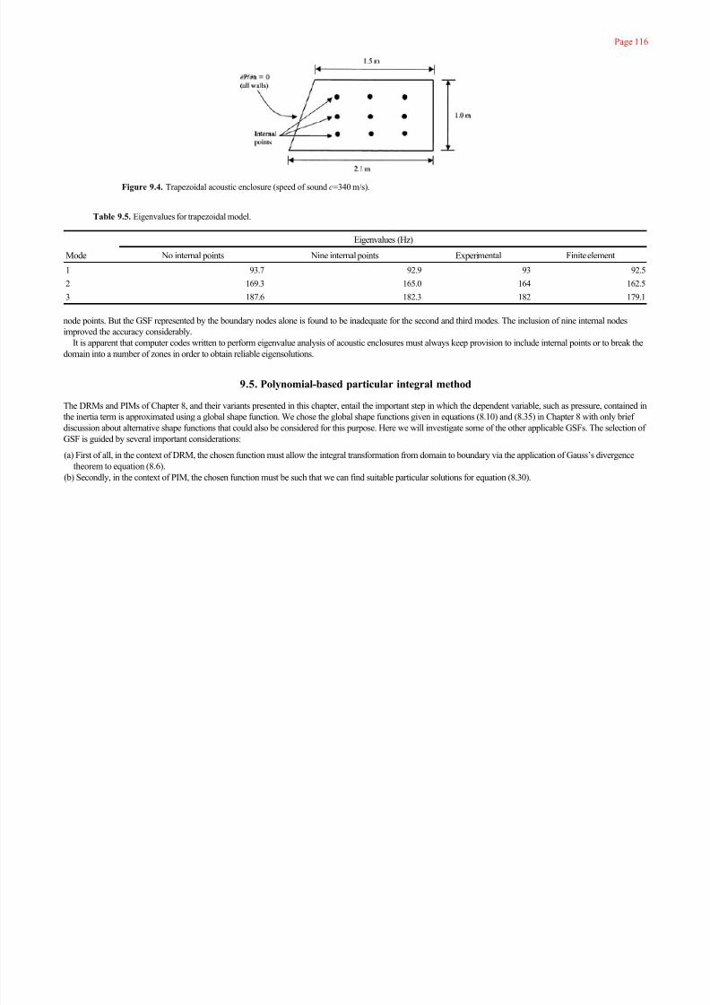
7/17/2019 The Boundary Element
http://slidepdf.com/reader/full/the-boundary-element 129/201
Page 116
Figure 9.4. Trapezoidal acoustic enclosure (speed of sound c=340 m/s).
node points. But the GSF represented by the boundary nodes alone is found to be inadequate for the second and third modes. The inclusion of nine internal nodesimproved the accuracy considerably.
It is apparent that computer codes written to perform eigenvalue analysis of acoustic enclosures must always keep provision to include internal points or to break the
domain into a number of zones in order to obtain reliable eigensolutions.
9.5. Polynomial-based particular integral method
The DRMs and PIMs of Chapter 8, and their variants presented in this chapter, entail the important step in which the dependent variable, such as pressure, contained in
the inertia term is approximated using a global shape function. We chose the global shape functions given in equations (8.10) and (8.35) in Chapter 8 with only brief
discussion about alternative shape functions that could also be considered for this purpose. Here we will investigate some of the other applicable GSFs. The selection of
GSF is guided by several important considerations:
(a) First of all, in the context of DRM, the chosen function must allow the integral transformation from domain to boundary via the application of Gauss’s divergence
theorem to equation (8.6).
(b) Secondly, in the context of PIM, the chosen function must be such that we can find suitable particular solutions for equation (8.30).
Table 9.5. Eigenvalues for trapezoidal model.
Eigenvalues (Hz)
Mode No internal points Nine internal points Experimental Finite element
1 93.7 92.9 93 92.5
2 169.3 165.0 164 162.5
3 187.6 182.3 182 179.1

7/17/2019 The Boundary Element
http://slidepdf.com/reader/full/the-boundary-element 130/201
Page 117
(c) And finally, the functions must be chosen such that they produce sufficiently accurate eigensolution, and at the same time, can be generated in a computationally
efficient manner.
The inertia term approximation with GSFs used in equations (8.10) and (8.35) can be improved by the addition of constant and/or higher order terms to the shape
functions [116]. The shape function C(x, ξ m ), given in equation (8.10), can be generalized further to contain terms with positive powers of the distance between the
field and source points, r(x, ξ m ), rather than just the linear term [ R−r(x, ξ
m )] alone. Here, we consider a complete polynomial as a possible choice for the GSF. So, the
acoustic pressure that appears in the inertia term can be represented by [135]:
where C m
(x) is a set of polynomial functions and Φm
is the vector of unknown coefficients associated with these polynomial functions. However, the above equation is
an infinite series. On practical grounds, we replace it by a finite series containing a finite number of polynomial terms. For example, a complete second order polynomial
expression in 2-D and 3-D spaces can be written down as finite series equations shown below:
Here, the total number of unknown coefficients is six for 2-D and 10 for 3-D spatial representations of the pressure in the domain. When the linear GSF [ R−r(x, ξ m
)] is
used to approximate the dependent variable in the inertia term using the boundary nodes as collocation points, the number of unknown coefficients (Φm
) equals the
number of boundary nodes, N . This leads to a square matrix [C], in equation (8.17), which is inverted [eqn. (8.18)] to solve for the unknown coefficients vector Φ.
Here, when polynomials in equation (9.32) or (9.33) are used to approximate the dependent variable, the number of unknown coefficients remains six for 2-D and 10
for 3-D. This usually will lead to a rectangular [C ] matrix since, typically, there will be more collocation points (i.e. boundary nodes) than the unknown coefficients
where the dependent variable is collocated.
Therefore, a least square regression approach needs to be employed to compute the unknown coefficients in this over-determined system. The least square method
may be employed in the following way:
(a) Representing the collocation of pressure, we can write the relations given in equations (9.32) and (9.33) in matrix form as [P ]=[C ]Φ. This is same as equation
(8.17), except here [C ] is a rectangular matrix.
(b) Pre-multiplying this equation by [C ]T yields [C ]T [P ]=[C ]T [C ]Φ. The resulting matrix [C ]T [C ] is square and, therefore, can be inverted. The product [C ]T
[C ] yields a 6×6 matrix for 2-D and 10×10 for 3-D for the second-order polynomial functions considered here. For the linear GSF based approximation, the [C]
matrix in equation (8.17) is of size N × N, where N is the number of boundary nodes.
(9.31)
(9.32)
(9.33)

7/17/2019 The Boundary Element
http://slidepdf.com/reader/full/the-boundary-element 131/201
Page 118
(c) Now, the coefficient vector Φ is computed as:
Notice here that the size of the matrix to be inverted is much smaller (either 6×6 or 10×10) compared to the case of linear GSFs.
We can now proceed to formulate the algebraic eigenvalue problem using PIM as presented in Section 8.3.1. To this end, we substitute the polynomial-based
approximation from equation (9.31) into equation (9.3) to obtain:
where C m(x) are the polynomial terms, ,found in equations (9.32) for 2-D and (9.33) for 3-D. We can now solve for the particular solution P I(x):
M =6 for 2-D and 10 for 3-D for the second-order polynomial functions used here. Dm(x) for 3-D are given below:
The normal derivative of this particular solution can be found as:
T m(x)are given below:
(9.34)
(9.35)
(9.36)
(9.37)
(9.38)
(9.39)

7/17/2019 The Boundary Element
http://slidepdf.com/reader/full/the-boundary-element 132/201
Page 119
In the above particular solution expressions, d =3 for 3-D (d =2 for 2-D), ni are the components of outward normal at the boundary nodes. The solution for the 2-D
case can be deduced from above by putting i=1,2 and setting the third-direction components to zero. After boundary discretization, the above particular solutions can
be written in matrix form as in equation (9.8) with the difference that [D] and [T ] are now rectangular matrices. Substitution of these matrix equations for particular
solution and its derivative into equation (9.5) leads to equation (9.9). We can then eliminate the unknown coefficients Φ from equation (9.9) using (9.34) and arrive at
the following eigenvalue problem:
As before, after applying the boundary conditions, equation (9.40) can be cast into a generalized algebraic eigenvalue problem, [A]xi =k 2[B]x
i , where x
i are the
eigenvectors [P i , Q
i ], Q
i ], k
i are the eigenvalues (k
i=ω
i/c) and Q
i=∂ P
i/∂n.
Next, we will illustrate the use of this polynomial-based PIM with a number of example problems. In all the examples the geometry, pressure, and particular solution
variables are approximated using isoparametric quadratic shape functions. The boundary walls for all the presented problems are considered as acoustically hard
surfaces (Q=∂ P /∂n=0) and the speed of sound is taken as 340 m/s. The eigenvalue problem presented by the above equation was solved using EISPACK [182]
employing an extraction technique based on the Arnoldi’s algorithm [127,135].
9.5.1. Examples of polynomial-based particular integral method
Example 9.4: Two-dimensional rectangular acoustic cavity
This impedance tube problem has been presented earlier (see example problems 8.1 and 9.1). Here eigensolutions from polynomial shape function (PSF)
approximation are compared against those from GSF approximation. The results are shown in Table 9.6 where the analytical solutions are also noted. Since this is
essentially a one-dimensional problem, the break-up of the domain into a number of regions does not have any perceptible influence on the solution.
Example 9.5: Automotive compartment with and without seats
This problem was presented in Chapter 8. See example problem 8.3 and Figures 8.3 through 8.6 and Table 8.2. Here Table 9.7 compares the GSF approximation
solutions with those from PSF approximation. Finite element and experimental results are also shown in the table. Since the method based on PSF approximation
requires inversion of a much smaller matrix, it requires significantly less CPU time compared to the GSF approximation based technique.
(9.40)
Table 9.6. Acoustic resonant frequencies (Hz) for impedance tube.
GSF PSF
Mode Analytical One region Two regions Four regions Two regions Four regions
1 4.25 4.24 4.24 4.22 4.25 4.25
2 8.5 8.46 8.48 8.45 8.73 8.51
3 12.75 12.68 12.69 12.70 13.32 12.80
4 17.0 16.88 16.89 16.97 18.17 17.73

7/17/2019 The Boundary Element
http://slidepdf.com/reader/full/the-boundary-element 133/201
Page 120
Table 9.7. Acoustic resonant frequencies (Hz) for a hatchback car interior compartment.
Without seats With seats
GSF GSF
Mode Experimental FEM One region Four regions PSF Four regions Experimental FEM One region Four regions PSF four regions
1 60 68 69 72 73 53 50 48 49 49
2 110 105 104 110 111 — 79 75 78 78
3 135 152 153 155 155 — 125 116 122 129
4 — 179 190 186 193 — 163 157 159 166
Table 9.8. Acoustic resonant frequencies (Hz) of rectilinear cavity.
GSF
Mode Analytical One region Four regions PSF Four regions GSF Four regions PSF Four regions
1 10.625 10.607 10.591 10.634 10.505 10.634
2 21.25 21.120 21.162 21.834 21.057 21.291
3 31.875 31.590 31.619 33.840 31.659 32.098
4 42.5 41.947 41.938 46.440 42.241 44.524

7/17/2019 The Boundary Element
http://slidepdf.com/reader/full/the-boundary-element 134/201
Page 121
Example 9.6: Three-dimensional rectilinear acoustic cavity This is a 3-D version of the impedance tube problem and has the closed form analytical solution given by equation (8.23), that is, although the geometry is 3-D, it is still
essentially a one-dimensional problem. Let us consider a 16 meter long tube with a one meter square cross-section. The problem is solved using polynomial based
shape function approximation as well as GSF approximation. The results along with the analytical solutions are presented in Table 9.8. The tube is treated as a single-
region and four-region BE domain. As noted earlier, since this is a 1-D problem, the use of multiple regions does not act in favor of improving the eigensolution.
Example 9.7: Three-dimensional truck-cab acoustic model
See example 8.4 for the geometric description of this 3-D acoustic eigenvalue problem. Here two different BE models are used to solve the eigenproblem. The first
case is a single-region BE model as described in example 8.4. In the second case, the 3-D cavity is broken into three BE zones: each of the end two zones is
discretized using 30 boundary elements and 90 nodes whereas the middle zone is modeled using 25 elements and 75 nodes. Table 9.9 lists the results, where the results
from GSF based approximation as well as finite element method (FEM) [177] are also tabulated.
9.6. Multiple reciprocity method (MRM)
The MRM can be looked upon as an extension of the idea of DRM presented in Section 8.2. The purpose of DRM and MRM is to transform domain integrals arisingfrom the application of BEM to free-vibration problems, problems with body forces, and treatment of certain classes of non-linearities. The DRM requires that the
dependent variable appearing inside the inertia term be approximated by functions having certain qualities so that Gauss’s divergence theorem may be applied to
transform the domain integral to boundary integrals. Here, MRM eliminates the need to approximate the dependent variable. Instead, in this method, Gauss’s
divergence theorem is repeatedly applied to the domain integral term using higher order Green’s functions until the domain term becomes negligible [138–140]. Let us
consider the Poisson’s equation for the purpose of illustrating the method:
where b0
(x) is a function representing body force. If then we can write the following integral
Table 9.9. Acoustic resonant frequencies (Hz) of a truck-cab.
Mode FEM GSF One region PSF One region GSF Three regions PSF Three regions
1 67 72 78 72 72
2 82 85 92 85 91
3 105 109 124 111 119
(9.41)

7/17/2019 The Boundary Element
http://slidepdf.com/reader/full/the-boundary-element 135/201
Page 122
equation:
The concern here is to transform the domain integral body force term into boundary integral. To this end, let us consider the following sequence of body force functions
and fundamental solutions:
These relationships make the repeated application of Gauss’s divergence theorem to the domain integral possible. The series of particular solutions of equation (9.44)
are known as the higher-order fundamental solutions. Making use of these series of functions, the domain integral term of equation (9.42) can be evaluated as:
The assumption here is that if we apply the Gauss’s divergence theorem a sufficient number of times, then the domain integral term of equation (9.45) will become
negligible. For example, if the body force term b0(x) is a polynomial of x, b1(x), b2(x),…, then the repeated application of divergence theorem will diminish their order.
In that case, we can evaluate the domain integral with sufficient accuracy by a finite number of terms. The higher-order fundamental solution series (x)for equation
(9.44) are given by:
In the case of the Helmholtz equation, we have b0
(x)=k 2 P(x) so that b1
(x)= and so on, which leads to:
We can substitute this into equation (9.45) to evaluate the domain integral term for the Helmholtz equation and as a result we can rewrite integral equation (9.42) for the
Helmholtz equation in the following manner:
(9.42)
(9.43)
(9.44)
(9.45)
(9.46)
(9.47)
(9.48)
(9.49)

7/17/2019 The Boundary Element
http://slidepdf.com/reader/full/the-boundary-element 136/201
Page 123
It can be seen from the fundamental solutions (9.46) and (9.47) that the leftover domain integral term in equation (9.49) will tend to zero for sufficiently large N . We,
therefore, obtain the boundary-only integral equation representation for the Helmholtz equation:
Discretizing the boundary Γ and performing integration on the boundary element segments, the integral equation can be converted to:
where Q=∂ P /∂n. After applying specified homogeneous boundary conditions into equation (9.51) and assembling the matrix, one obtains:
where:
Kamiya and Andoh [141] solved equation (9.52) using Newton-Raphson iteration along with LU decomposition [183]. Note that the matrices [A0 ]···[A
N ] do not
contain the frequency parameter k and, therefore, need not be formed at each iteration. Additionally, with this technique, internal collocation points are not required for
an accurate evaluation of the resonant frequencies. Since it is an iterative technique, the solution procedure requires an initial rough estimate of the frequencies at the
start of the iteration process. The Newton-Raphson solution technique may be looked upon as an enhanced determinant search method (DSM).
Example 9.8: An illustration of MRM: a rectangular parallelopiped acoustic cavity problem
As an example of the application of MRM with Newton-Raphson/LU iteration procedure, consider a rectangular parallelopiped [143], shown in Figure 9.5. The
dimensions, boundary conditions and boundary discretizations are shown in the figure. Two different discretizations, shown in Figures 9.5(a) and 9.5(b), respectively,
are considered: one with 24 constant elements and the other with 94 constant elements. The analytical solution for this problem is given by:
The results of the analysis are presented in Table 9.10 where the closed-form solutions are also shown. The maximum error is seen to diminish from five per cent to two
per cent as the discretization gets finer.
(9.50)
(9.51)
(9.52)
(9.53)
(9.54)

7/17/2019 The Boundary Element
http://slidepdf.com/reader/full/the-boundary-element 137/201
Page 124
Figure 9.5. A rectangular parallelopiped acoustical cavity. (a) 24 elements; (b) 94 elements.
9.6.1. MRM and matrix augmentation As noted above, MRM does not lead to an algebraic eigenvalue formulation, but it rather falls in the category of enhanced DSM. However, we can use a matrix
augmentation procedure [142] to cast equation (9.52) into a generalized eigenproblem. To facilitate it, let us rewrite equation (9.52) in the following manner with the
help of equation (9.53):
Table 9.10. Results for rectangular parallelopiped acoustical cavity.
(m, n, t) Analytical solution MRM 24 elements Error (%) MRM 94 elements Error (%)
(0, 0, 0) 1.57 1.64 4.5 1.59 1.3
(0,1,0) 4.23 4.44 5.0 4.28 1.2
(0, 0, 1) 4.71 4.76 1.1 4.71 0.0
(1,0,0) 5.47 5.60 2.4 5.58 2.0
(9.55)

7/17/2019 The Boundary Element
http://slidepdf.com/reader/full/the-boundary-element 138/201
Page 125
where the right-hand side of equation (9.52) is basically a null vector and it is set equal to zero in equation (9.55). Let us also define k 2=λ and introduce a series of
vector relationships as follows:
If we put i=0 in the above relation, we get the following:
The equations (9.56) and (9.57) can be turned into a recursive relation of the form:
Equations (9.55) and (9.58) can be combined into a single augmented matrix equation:
The augmented matrices and [Ā] and[Â], the augmented vector are then given by:
Now the problem could be solved using generalized eigensolvers. As can be seen from the matrices (9.60) and (9.61), the order of the matrices to be solved has gone
up significantly, requiring more computer time and storage. While it was motivated by the apparent advantage of being able to solve the eigenproblem using a
generalized eigensolver as a black-box, the matrix augmentation procedure may defeat the very purpose of using boundary-only discretization technique in the first
place. The only remaining advantage of BE eigenvalue formulation using this approach will then be in the preparation of meshes for complex geometries since putting
internal points or breaking up into regions is not needed for MRM.
(9.56)
(9.57)
(9.58)
(9.59)
(9.60)
(9.61)
(9.62)

7/17/2019 The Boundary Element
http://slidepdf.com/reader/full/the-boundary-element 139/201
Page 126
Figure 9.6. A rectangular acoustical cavity.
Let us solve a 2-D problem for illustration. The problem is a 0.9×0.6 rectangular acoustical cavity with mixed boundary conditions, as shown in Figure 9.6. Two
discretizations, one with 26 constant elements and the other with 44 constant elements, were used to solve the problem. The closed-form analytical solution for this
problem is given by:
The results are presented in Table 9.11 where the analytical solutions are compared against those obtained using (a) MRM with Newton/LU iterations and (b) MRM
with matrix augmentation [143]. Both results agree very well with the closed-form solutions. The second row in Table 9.11, shown with an asterisk, is a fictitious
eigenvalue, which is not predicted by the closed-form solution. According to Kamiya et al. [143], the fictitious eigenvalues correspond to the zeros of the determinant
of the matrix [B(k)] in equation (9.52). In practical applications, again, a robust method of detecting these spurious modes will have to be developed for this method to
be useful.
Chen and co-workers (see [155]) observed that the MRM formulation, presented above, deals only with the real part of the complete complex-valued MRM
formulation. Since the formulation leaves out the imaginary part, it results into insufficient number of constraints for the eigenequation, introducing spurious roots into theeigenproblem. Chen and his co-workers used residual method and singular value decomposition technique [155] to filter out these spurious modes from the
eigensolution.
Table 9.11. Results for rectangular acoustical cavity.
MRM with matrix augmentation MRM with LU/Newton
26 Elements 44 Elements 26 Elements 44 Elements Analytical solution
1.75 1.75 1.74 1.74 1.75
4.81* 4.81*
5.25 5.24 5.25 5.25 5.24
*Fictitious eigenvalue.
(9.63)

7/17/2019 The Boundary Element
http://slidepdf.com/reader/full/the-boundary-element 140/201
Page 127
9.7. Series expansion methods (SEM) with matrix augmentation
It is clear that the use of a fundamental solution which rigorously corresponds to a governing differential equation leads to an eigenvalue formulation with the frequency
parameter implicitly embedded into the system matrices. See for example the characteristic equations (6.51) and (6.55). This forced us to use direct DSM as described
in Section 6.4.1. In Section 6.4.2, we also presented an enhanced DSM in which we expanded the characteristic equation into a series. The frequency parameters are
factored out of the system matrices by this expansion [see eqns. (6.60) and (6.61)]. We can now use a matrix augmentation process, as outlined in the last section, to
recast this series equation into a generalized eigenproblem, such as equation (9.59).
It can be shown that the series equation, viz., equation (6.60), is equivalent to equation (9.52) derived using MRM [143,184,185]. Note that the SEM [144] uses a
fundamental solution for the Helmholtz equation for acoustic problems, whereas the MRM uses higher-order fundamental solutions for the Laplacian portion ofHelmholtz equation for the same problem.

7/17/2019 The Boundary Element
http://slidepdf.com/reader/full/the-boundary-element 141/201
Page 128
This page intentionally left blank.

7/17/2019 The Boundary Element
http://slidepdf.com/reader/full/the-boundary-element 142/201
Page 129
Chapter 10
Acoustic Fluid-Structure Interaction Problems
10.1. Introduction
In this chapter the eigenvalue analysis of acoustic fluid-structure systems encountered in acoustical cavities with flexible structure boundaries, such as a fluid-filledcontainer or an automobile cabin enclosure, is considered. In applications involving acoustic cavities with flexible wall boundaries, the computation of the structural and
cavity resonance involves solving the acoustic fluid-structure eigenproblem. Typically, the finite element method (FEM) is used to solve such fluid-structure coupled
eigenproblems [178,186]. However, when the problem size gets larger, as in the case of a structure in contact with a large extent of fluid, the finite element (FE)
discretized stiffness and mass matrices of the coupled problem become very large, significantly increasing the eigenvalue computation time. In these situations, the
boundary element method (BEM) becomes attractive since the discretization of the acoustic fluid domain leads to placing fluid nodes and elements only on the wetted
surface of the structure, thus leading to relatively smaller size matrices for the coupled problem. However, boundary element (BE) matrices are non-symmetric; so also,
are the pressure-displacement based finite element matrices even though the system sub-matrices are symmetric. Efficient methods of computing the eigenvalues and
eigenvectors of non-symmetric eigenvalue problems will be presented in Chapter 11.
We will formulate the fluid-structure eigenproblem using boundary element discretization of the fluid and finite element discretization of the structure. For the fluid
domain, any of the acoustic fluid boundary element eigenanalysis formulations such as Dual Reciprocity (DRM), Multiple Reciprocity (MRM) or Particular Integral
Method, (PIM) presented in Chapters 8 and 9 can be used. For the structure, finite element eigenformulation is employed. In Section 9.2.3, the boundary element-finite
element fluid-structure formulation was briefly outlined. However, we presented only the acoustic cavity eigenanalysis results there. In this chapter, eigenanalysis of the
fluid-structure problem is presented in detail. We also present a number of illustrative problems where we compute the eigenfrequencies of structures in contact with
fluid.
Boundary element-finite element coupled fluid-structure analysis is quite commonly employed in the frequency domain analysis of fluid-structure problems, where thecoupled system response to excitation forces is computed as outlined in Section 5.2.1. Setting the excitation forces to zero, it is also possible to solve for the natural
frequencies of the coupled problem using the method of determinant search to compute the eigenfrequencies and modes as shown in Sections 6.2 and 6.4. In this
chapter,

7/17/2019 The Boundary Element
http://slidepdf.com/reader/full/the-boundary-element 143/201
Page 130
however, the boundary element-finite element coupled problem is set up as an algebraic eigenvalue problem in order to extract the eigenfrequencies and mode shapes
of the fluid-structure system. To our knowledge, the authors of this book made the first ever attempt to perform a boundary element-finite element coupled algebraic
eigenvalue analysis for acoustic fluid-structure problem [137].
10.2. Boundary element-finite element coupled eigenanalysis of fluid-structure system
We consider a fluid-structure system shown schematically in Figure 10.1. The fluid domain is confined and has two different types of boundaries. One portion of the
fluid boundary is acoustically hard and the other portion is in contact with a flexible structure. For the time harmonic acoustic pressure, p= P e jωt , in the fluid, the wave
equation reduces to the Helmholtz equation where P is the pressure amplitude, k =ω/c is the wave number, c is the speed of sound in the fluid andω isthe circular frequency of pressure oscillations. The boundary conditions of the fluid boundary in terms of the pressure amplitude can be written as:
Acoustically hard boundary:
Fluid-Structure Interface:
where u is the displacement vector of the structure at the interface, n is the unit normal of the interface drawn into the structure, and ρ is the fluid density and “·”
represents the dot product.
The boundary element algebraic eigenvalue problem of the Helmholtz equation for the fluid can be formulated using either the DRM or the PIM presented in Chapter
8. Both the methods yield the same end result. The reader is referred to Chapter 8 for detailed derivations of the algebraic eigenvalue problem using these methods.
The
Figure 10.1. Acoustic fluid-structure problem.
(10.1a)
(10.1b)

7/17/2019 The Boundary Element
http://slidepdf.com/reader/full/the-boundary-element 144/201
Page 131
application of any of these methods leads to the following equation [eqn. (8.16) in DRM, eqn. (8.52) in PIM)]:
The matrices appearing in this equation are defined in Chapter 8. Here, it is possible to replace the fictitious function vector Φ in favor of the physical variable P
using equation (8.17). However, here we choose to retain Φ as the unknown vector in order to avoid the inversion of the [C] matrix, as shown in the Fictitious
Function Method (FFM) in Section 9.2. Once Φ is known, which will be part of the eigenvector solution, P can be recovered using equation (8.17). For acoustic
cavities with hard boundaries all around, the algebraic eigenproblem is obtained by setting ∂ P /∂n=0 in equation (10.2). When the boundary is not hard, i.e., when the boundary is flexible, the fluid-structure interface condition ∂ P /∂n= ρω2
u·n is used to couple the acoustic domain to the oscillating structure.
If we denote the x and y components of the unit normal, n, as n x
and n y , we can write the boundary integral matrix equation (10.2) in terms of the interface nodal
displacements u and nodal fictitious functions Φ as unknowns.
The finite element structural dynamic equation can now be written taking into account the pressure force of the acoustic fluid acting on the structure [186].
The matrix [R] represents the surface area at the interface, and [K s
] and [M s
] are the structural stiffness and mass matrices, respectively. Substituting for P from
equation (8.17), the structural dynamic equation (10.4) is rewritten as:
The boundary element-finite element coupled eigenproblem can be written combining equations (10.3) and (10.5):
The matrices of the eigenproblem given in equation (10.6) are non-symmetric. Furthermore, the acoustic fluid boundary element matrices in the bottom row are fully
populated. The effectiveness of the fluid-structure eigenanalysis will, therefore, depend upon an efficient method for extracting the eigenvalues of this non-symmetric
system. In Chapter 11, we will present eigenvalue computational procedures based on the Lanczos method for non-symmetric matrices. The Lanczos subspace method
is a powerful computational tool for extracting a few eigenvalues of a large non-symmetric eigenproblem within a specified range of its eigenvalue spectrum. Usually, forthe fluid-structure problem the lowest resonant frequencies are of interest, and the Lanczos method is well suited for that.
As pointed out earlier, the pressure-displacement based finite element-finite element coupled eigenproblem is also non-symmetric, and will involve much larger sized
fluid matrices than the boundary element-finite element eigenproblem for the same given fluid-structure analysis. Therefore, eigenproblem formulation using the
(10.2)
(10.3)
(10.4)
(10.5)
(10.6)

7/17/2019 The Boundary Element
http://slidepdf.com/reader/full/the-boundary-element 145/201
Page 132
Figure 10.2. Impedance tube coupled to spring-mass oscillator ( L=40m, W =2m, K =60 N/m, M =0.25 kg, ρ=1.12 kg/m3, c=340 m/s).
boundary element-finite element coupled analysis approach, given by equation (10.6), would be relatively more efficient.
10.2.1. Application of fluid-structure eigenformulation
The example problems in this section are intended to show the application of fluid-structure eigenanalysis, and to compare the effectiveness of the boundary element-
finite element eigenanalysis with respect to the finite element-finite element coupled eigenanalysis [178,186]. First, through a simple example, we validate the boundary
element-finite element coupled formulation by comparing the computed results with the theoretical solution. Then, practical applications of the method are illustrated by
considering two representative fluid-structure problems.
Example 10.1: Impedance tube coupled to spring-mass oscillator
This one-dimensional (1-D) problem is a spring-mass oscillator placed at one end of an acoustic tube as shown in Figure 10.2. The other end of the air-filled tube is
closed. Tube dimensions are chosen with a large length to width ratio, L/ W ,
so that the coupled system behaves, essentially, as a 1-D acoustic tube oscillator in the
lower range of frequencies that we are interested. The mass, M, and stiffness, K, of the oscillator are chosen to be light and soft compared to the mass and stiffness,
respectively, of the air column in the tube.
For such an oscillator-tube combination the resonant frequencies are given by an approximate expression [187] of the form:
This approximate expression is derived from the exact frequency expression:
The coefficients a and b are the mass and stiffness ratios given by M/(ρAL) and KL/(ρAc2 ), respectively, where A is the cross-section area of the tube and L is its
length. ρ and c are the density of the fluid and the speed of sound in the fluid, respectively. The theoretical frequencies listed in Table 10.1 have been evaluated using the
exact frequency expression given by equation (10.8).
For the boundary element-finite element coupled eigenanalysis, the fluid domain boundary is discretized into 36 linear boundary elements as shown in Figure 10.2.
The mass M which acts as the piston is modeled using stiff beam finite elements, and the spring K is modeled by a discrete stiffness element. The eigenvalues of the
unsymmetric eigenvalue problem were extracted using the Lanczos eigenvalue solver, presented in Chapter 11, and the eigenfrequencies are listed in Table 10.1. The
computed frequencies agree very well with the theoretical frequencies. Also, presented in Table 10.1 are
(10.7)
(10.8)

7/17/2019 The Boundary Element
http://slidepdf.com/reader/full/the-boundary-element 146/201
Page 133
the eigenfrequencies computed using the finite element-finite element coupled analysis using 16 bilinear two-dimensional (2-D) acoustic fluid elements, available in the
ANSYS program [160], along the length of the tube.
Example 10.2: Fluid- illed cylindrical shell
This is a practical example illustrating the use of fluid-structure eigenanalysis to predict the effect of fluid in reducing the resonant frequencies of the structure. Figure
10.3a shows the cross-sectional dimensions of a cylindrical shell filled with water. Since the cylinder is assumed to be infinitely long, the problem is modeled in 2-D to
compute the resonant frequencies of the coupled problem. This shell is modeled using two-noded beam finite elements along the circumference and the boundaryelement nodes of the fluid inside coincide with the finite element nodes of the shell. The computed frequencies along with the analytical frequencies are presented in
Table 10.2.
The first fifteen computed eigenmodes of the shell are shown in Figure 10.3c. The analytical frequencies were computed from the frequency expression for the fluid-
filled shell given in the reference by Yu [188]. They differ slightly from those reported by Yu because calculations were performed using the British System of units in
the reference by Yu, whereas here SI units are used and the resulting rounding of the numbers in the conversion process could be attributed to the difference.
In the boundary element discretization of the fluid, four different cases were investigated to study the effect of putting internal points in the fluid domain. As was
pointed out in Section 9.4 [131], the boundary element eigenanalysis invariably needs internal points to ensure that eigenmodes with purely interior nodal lines are not
missed. For example, in the case of a circular acoustic fluid domain with hard boundary, eigenmodes that have concentric ring shaped pressure contours will be missed
if no internal point is used. In this example, therefore, we solve with and without internal points to confirm this observation in the case of fluid-structure problems. From
the results presented in Table 10.2, it is seen that when no internal points are used the breathing mode of the shell, mode 13, is missed and as more internal points are
added, the accuracy of the frequencies improves. In order to compare results, finite element-finite element coupled analysis of the problem was performed using the 2-
D acoustic fluid elements in the ANSYS program [160]. The finite element mesh used is shown in Figure 10.3b and the computed frequencies are listed in Table 10.2.
Table 10.1. Resonant frequencies of the impedance tube coupled to oscillator (Hz).
Mode Theoretical BE-FE FE-FE
1 2.127 2.1167124 2.1199338
2 6.360 6.3803167 6.3801376
3 10.597 10.674617 10.701530
4 14.835 15.054761 15.125397
5 19.073 19.536871 19.693362
6 23.211 24.205379 24.446556
7 27.549 29.067250 29.423477
8 31.787 34.244301 34.655527
9 36.025 39.689099 40.158698
10 40.263 45.558443 45.919184

7/17/2019 The Boundary Element
http://slidepdf.com/reader/full/the-boundary-element 147/201
Page 134
Figure 10.3. Fluid-filled shell model and mode shapes (shell: Young’s modulus E =2.068×10¹¹ N/m2, density ρs=2403 kg/m3, Poisson’s
ratio v=0, thickness t =0.102 m; Water: density ρ=1000 kg/m3, speed of sound c=1500 m/s). (a) boundary element model; (b)finite element model; (c) shell mode shapes.
Example 10.3: Loudspeaker-box problem
This is a problem chosen to represent a high-fidelity loudspeaker enclosure design application encountered in audio engineering. The problem configuration considered
is shown in Figure 10.4, where the loudspeaker-box assembly is modeled in 2-D. The semi-circular shell represents the driver surface and it is fixed on to the box
which represents the loudspeaker enclosure, the inside of which is filled with air.
This problem is a representative example of a fluid-structure problem encountered in the acoustical design of a driver-enclosure. Material properties of the box and
the shell are chosen to represent a wooden enclosure with a driver made of cloth reinforced plastic, respectively. The property values shown in the Figure 10.4 are
taken from reference [189]. Jones et al. [190] point out that a typical material used to construct the driver cone is cobex, which is relatively stiff and light. Since the
property values of cobex are not readily available, we have used cloth reinforced plastic which exhibits similar property characteristics.

7/17/2019 The Boundary Element
http://slidepdf.com/reader/full/the-boundary-element 148/201
Page 135
Table 10.2. Resonant frequencies of the fluid-filled shell (Hz).
Theory
Free parameter in the freq. expression (n=0, 1, 2, …)
BE-FE (with different no. of internal points)
Mode Freq. 0 1 5 9 FE-FE Freq. of shell w/o fluid inside FE
1, 2 2 25.157 25.158 25.158 25.160 25.159 25.163 47.160
3,4 3 78.277 79.110 79.105 79.108 79.115 79.176 133.27
5, 6 4 161.10 164.72 164.72 164.73 164.78 165.13 255.23
7, 8 5 274.02 283.66 283.66 283.67 283.69 284.91 412.20
9,10 6 416.56 436.71 436.71 436.73 436.73 439.45 603.76
11,12 1 449.64 553.91 553.90 490.58 466.14 445.64 —
13 0 505.59 — 511.57 514.62 515.43 495.06 829.66
14, 15 7 587.41 624.00 624.00 624.00 624.00 628.78 939.81

7/17/2019 The Boundary Element
http://slidepdf.com/reader/full/the-boundary-element 149/201
Page 136
Figure 10.4. Loudspeaker enclosure model and mode shapes (box: Young’s modulus E b
=1×10⁹ N/m2, density ρ b
=450 kg/m3, thickness
t b
=0.025 m; Shell: E s=2×10⁹ N/m2, ρ
s=1500 kg/m3, t
s=0.0005 m; air: ρ=1.12 kg/m3, speed of sound c=340 m/s). (a) boundary
element model; (b) finite element model; (c) Mode shapes.
The eigenfrequencies of the loudspeaker box assembly are listed in Table 10.3 and the mode shapes are shown in Figure 10.4c. Boundary element-finite elementcoupled analysis shows good agreement with the finite element-finite element results. In the case of boundary element-finite element coupled analysis, the frequencies
computed with and without internal points are quite close to each other indicating that, within the frequency range of the six modes presented, the problem has no
modes that have mode shapes with nodal lines purely interior to the boundary. However, for routine

7/17/2019 The Boundary Element
http://slidepdf.com/reader/full/the-boundary-element 150/201
Page 137
computations it is recommended that internal points are always used in order to ensure capturing all of the eigenmodes of a given problem. Also listed in Table 10.3 are
the frequencies of the loudspeaker box without air filled inside for comparing the effect of air in the enclosure. It is evident that the air inside the enclosure significantly
affects the resonant frequencies of the loudspeaker box assembly.
10.3. Acoustic eigenproblem for enclosures with dissipative boundaries
The damped system resonant modes of acoustic cavities, such as the automobile passenger cabin lined with foam and fibrous type material, is considered in this section.
In the previous section we have dealt with acoustic enclosure boundaries which are acoustically hard where there is no loss of energy at the boundary walls and the
boundary condition is given by ∂ P /∂n=0. We have also dealt with the case in which the enclosure boundary is a vibrating structure in contact with the acoustic fluid
where the boundary condition becomes ∂ P /∂n= ρω2u·n causing the energy to be transmitted to the vibrating structure. Another situation is where a part of theenclosure boundary may be completely open to the surrounding atmosphere and in equilibrium with the enclosure acoustic fluid. In this case the boundary condition is
simply given by P =0.
When the enclosure boundary is neither acoustically hard nor completely open to the atmosphere, the walls will absorb some energy and the rest will be contained
within the acoustic fluid medium. Here, we will present a simple yet effective technique to incorporate a dissipation term in the acoustic eigenvalue formulation to
account for the absorption of sound waves at the enclosure boundary walls. The boundary element discretization of acoustic cavities with sound absorption leads to a
non-symmetric damped eigenvalue system which is a quadratic eigenvalue problem. A Lanczos based algorithm designed to extract eigenvalues and modes of this non-
symmetric quadratic eigenproblem will be presented in Chapter 11. In order to be computationally efficient, the algorithm is designed to avoid the doubling of the
system matrices that is normally done in the matrix augmentation process used to linearize the quadratic eigenvalue problem.
A brief outline of the formulation is as follows: First, we will restate the acoustic boundary element eigenproblem equation without the dissipation term, as derived in
Chapters 8 and 9. Then, a simple method of incorporating boundary absorption into the acoustic wave equation discretization process will be shown. We will, next,
show how
Table 10.3. Resonant frequencies of the loudspeaker-box enclosure (Hz).
BE-FE
Mode Zero internal points Eight internal points FE-FE FE (enclosure without air inside)
1 1.177 1.177 1.178 1.313
2 2.691 2.691 2.692 2.791
3 5.053 5.053 5.056 3.377
4 6.562 6.562 6.562 5.299
5 7.867 7.879 7.875 6.670
6 8.591 8.618 8.623 8.231

7/17/2019 The Boundary Element
http://slidepdf.com/reader/full/the-boundary-element 151/201
Page 138
to incorporate the absorption term in the boundary element matrix equation. Finally, we will present several example problems, solved using the Lanczos algorithm for
non-symmetric quadratic eigenproblem. The Lanczos eigenvalue solver itself will be described Chapter 11.
10.3.1. Acoustic boundary element eigenproblem
As shown in earlier chapters, the acoustic wave equation governing the acoustic pressure p in a fluid is given by:
c is the speed of sound and t is the time. For the harmonic oscillations of pressure in the sound pressure wave problem considered, p= P e jωt . P is the pressure
amplitude,ω is the circular frequency and Substituting for p in equation (10.9), the Helmholtz equation governing the amplitude of pressure oscillations is
obtained.
The boundary element algebraic eigenvalue problem for this governing equation is given by [see eqns. (8.16), (8.52) and (10.2)]:
where the mass-type matrix [M]=([G][T]−[H][D]). This matrix equation represents the boundary element discretized, loss-less Helmholtz equation (10.10). In practical applications, however, the acoustic sound pressure partly dissipates as it reflects off of the bounding surfaces of an enclosure such as the carpeted flooring of a
room. In the following section, a method of incorporating the dissipation term in the discretized Helmholtz equation (10.11) is described.
10.3.2. Sound absorption at the boundary
Some amount of energy is almost always dissipated due to the absorption of sound at the boundaries of an acoustic domain. Especially, when different sound-absorbing
materials are used in the acoustic enclosure walls to deliberately dampen the sound, as shown in Figure 10.5, a way of modeling the sound absorption is needed. In
order to account for the dissipated energy, the reference by Craggs [191] shows a damped form of the Helmholtz equation (10.10). For the absorption of sound at the
boundaries of an acoustic cavity, a similar approach is used in the linear momentum equation that relates the fluid pressure gradient and the velocity at the boundary:
where ρ is the fluid density, v is the velocity vector, and n is the outward normal. To account for the energy dissipated at the boundaries, an absorption term is
introduced on the right-hand side of equation (10.12):
In the absorption term, the reason for using the velocity divergence ·v, as opposed to v as in Cragg’s paper, comes from the consideration of the consistency of units,
where the acoustic resistance R is in rayl (Ns/m3). In addition, Zienkiewicz and Newton [186] give the relationship ∂ p/∂n=−(1/c) ∂ p/∂t to account for the energy loss
due to the
(10.9)
(10.10)
(10.11)
(10.12)
(10.13)

7/17/2019 The Boundary Element
http://slidepdf.com/reader/full/the-boundary-element 152/201
Page 139
Figure 10.5. Acoustic cavity.
outbound pressure waves at an open boundary for plane wave situations. Since ∂ p/∂t is related to ·v via the conservation of mass equation:
of a compressible fluid, the boundary absorption term used in equation (10.13) would be appropriate. Substituting ·v from equation (10.14) into equation (10.13) the
pressure gradient at an absorbing boundary is written as:
β = R/ ρc is the non-dimensional absorption coefficient of the sound absorbing material at the boundary. The acoustic resistance R for foam and fibrous type material is
given as a function of frequency by Craggs [191].
For the harmonic oscillations in acoustical problems, the boundary pressure and velocity in equation (10.15) are represented in complex exponential form as p=
P e jωt and v=V e jωt , respectively. We are not using the boundary velocity here since the fluid-structure interface boundary is assumed to be stationary. The boundary
pressure gradient at a sound absorbing boundary is, then, obtained from equation (10.15) as:
At the absorbing boundary, however, the particle velocity normal to the surface may not be zero, since there exists a non-zero pressure gradient when β ≠0. Therefore,
the absorbing boundary can be described as “quasi-rigid” even though the boundary itself is not oscillating as in a fluid-structure coupling interface.
(10.14)
(10.15)
(10.16)

7/17/2019 The Boundary Element
http://slidepdf.com/reader/full/the-boundary-element 153/201
Page 140
Often in acoustical modeling, the impedance of an absorbing boundary is given. So, a relationship between the absorption coefficient β and the acoustic impedance Z
at the absorbing boundary can be obtained if the particle velocity v β
normal to the surface and the pressure are known. For the harmonically varying acoustic waves,
v β
=V β
e j(ωt +α), where V β
is the velocity magnitude and α is the phase angle of the velocity with respect to the pressure at the absorbing boundary. Using the relationship
between the pressure gradient and the particle velocity normal to the boundary, the expression for V β
can be found as V β
=j (∂ P /∂n) e−jα/(ρω). Solving for the pressure
P from equation (10.16), the impedance Z at the absorbing boundary is found by dividing P by V β
. The resulting expression for the impedance of the absorbing
boundary is Z =(ρc/β) e jα. It is evident from this relationship that the acoustic impedance of the absorbing boundary is complex-valued even though the absorption
coefficient β is real-valued. Therefore, in situations where the impedance of a boundary is known, the absorption coefficient to be applied can be calculated from this
expression as β = ρc/|Z|.The valid range of the absorption coefficient β is from zero to unity. When β =0, there is no energy loss at the boundary and the wall is rigid. For β =1, the entire
energy incident on the boundary is lost, which represents a boundary left open. For values of β that lie between zero and unity, part of the incident energy on the
boundary is lost and the rest is reflected back. Since β is non-dimensional, the question of whether its value can be greater than unity arises. In such a case R> ρc, which
implies that the absorbing boundary assists in taking energy out of the system. A plausible explanation can be given for a case where the acoustic medium beyond the
absorbing boundary has a characteristic impedance greater than ρc.
10.3.3. Absorption term in the boundary element eigenvalue matrix equation
Using the relationship in equation (10.16), the absorption in an acoustic cavity can be incorporated in the discretized boundary element equation (10.11). Equation
(10.16) is rewritten in terms of the nodal pressure gradients as follows:
When absorption material is used on a part of the boundary Γ1
, equation (10.11) can be written in partitioned form as:
Q1 and Q
2 denote pressure gradients at the absorbing and non-absorbing boundary nodes, respectively. Then, substituting from equation (10.17) into equation
(10.18), one obtains:
For the part of the boundary where there is no absorption, we assume acoustically hard boundary condition Q2 =0. Partitioning the matrix [C] of equation (8.17) as
in equation (10.18), we substitute for P 1 =[C
11 ]Φ
1+[C
12 ]Φ
2 in equation (10.19):
(10.17)
(10.18)
(10.19)
(10.20)

7/17/2019 The Boundary Element
http://slidepdf.com/reader/full/the-boundary-element 154/201
Page 141
Taking the coefficient − β into the matrix, and denoting the absorption matrix as and [K ]=−[H][C], equation (10.20) is rewritten as:
Equation (10.21) is the eigenvalue problem for the acoustic cavity with sound absorption. Defining the eigenvalues as λ i=j(ω/c), and the eigenvectors x
i =Φ, the
damped system eigenproblem to be solved is:
Equation (10.22) represents the generalized quadratic eigenvalue problem and, in general, will yield complex eigenvalues and eigenvectors. The computational
approach to solve this eigenvalue problem employing the Lanczos recursion scheme will be shown in the next chapter.
10.4. Examples of acoustic eigenproblem with sound absorption
We will consider two different acoustical cavities to demonstrate the effect of incorporating sound absorption in the acoustic boundary element eigenproblem. One is a
long impedance tube and the other is a square cavity. The boundary absorption method formulated in this chapter is also employed in the acoustic finite elements in the
ANSYS® general purpose program [160]. So, we compare the boundary element results with those of the finite element eigensolution results from the ANSYS
program in cases where a theoretical solution is unavailable. These examples, however, are not designed to quantitatively evaluate the absorption model that was shown
in the previous section.
Example 10.4
A long impedance tube of length to width ratio of 20, shown in Figure 10.6, is considered first. The tube wall at x= L is lined with a damping material of absorption
coefficient β . Since the aspect ratio is large, the first few undamped mode frequencies for this problem are given by the 1-D frequency expression f i=ic/(2 L), i=1,2,…,
∞. Table 10.4 shows the computed frequencies for three different values of absorption coefficient, β =0, 0.1 and 0.9, along with the undamped theoretical frequencies.
The acoustical resonant frequencies are the positive imaginary parts of the conjugate pair of eigenvalues computed.
For the undamped case, the frequencies computed by the BEM are in good agreement with the theoretical values. For the damped case, boundary element
frequencies are
Figure 10.6. Impedance tube with sound absorption (coefficients used: β =0, 0.1 and 0.9).
(10.21)
(10.22)

7/17/2019 The Boundary Element
http://slidepdf.com/reader/full/the-boundary-element 155/201
Page 142
Table 10.4. Acoustic resonant frequencies of impedance tube (Hz).
Absorption coefficient (β) Mode Theory BE FE
0 1 — −0.52727113E−05 −0.71259621E−07j 0.13906660E−05 −0.12434703E−04j
2 0+0j 0.52726372E−05 +0.71252287E–07j 0.13872865E−05 +0.12435437E–04j
3 — 0.00000000E+00 −4.2638284j 0.00000000E+00 −4.2568304j
4 0+4.25j 0.00000000E+00 +4.2638284j 0.00000000E+00 +4.2568304j
5 — 0.00000000E+00 −8.5312338j 0.00000000E+00 −8.5547171j
6 0+8.50j 0.00000000E+00 +8.5312338j 0.00000000E+00 +8.5547171j
7 — 0.00000000E+00 −12.905870j 0.00000000E+00 −12.935041j
8 0+12.75j 0.00000000E+00 +12.905870j 0.00000000E+00 +12.935041j
9 — 0.00000000E+00 −17.295136j 0.00000000E+00 −17.439604j
10 0+17.00j 0.00000000E+00 +17.295136j 0.00000000E+00 +17.439604j
0.1 1 0.15200149E−08 −0.56715029E−09j 0.16049927E−09 −0.73970017E−11j
2 −0.136+ 0j −0.13493624 +0.00000000E+00j −0.13573492 +0.00000000E00j
3 −0.13690670 −4.2638323j −0.13661136 −4.2567951j
4 −0.13690670 +4.2638323j −0.13661136 +4.2567951j
5 −0.13819908 −8.5310962j −0.13927476 −8.5546444j
6 −0.13819901 +8.5310962j −0.13927476 +8.5546444j
7 −0.14306932 −12.905832j −0.14382862 −12.934927j
8 −0.14306936 +12.905832j −0.14382862 +12.934927j
9 −0.14803122 −17.294763j −0.15044929 −17.439440j
10 −0.14803126 +17.294763j −0.15044929 +17.439440j
0.9 1 −0.74389602E−08 +0.53838077E–07j 0.46269145E−08 +0.49989396E–08j
2 −1.992+ 0j −1.9627462 +0.00000000E+00j −1.9886941 −0.57453587E−07j
3 −2.0131707 −4.2577669j −2.0084570 −4.2424017j
4 −2.0131707 +4.2577669j −2.0084570 +4.2424017j
5 −2.0478985 −8.4778993j −2.0699368 −8.5233054j
6 −2.0478985 +8.4778994j −2.0699370 +8.5233054j
7 −2.1870322 −12.858083j −2.1805021 −12.880197j
8 −2.1870323 +12.858083j −2.1805023 +12.880197j
9 -2.3191496 −17.111469j −2.3556919 −17.346699j10 −2.3191497 +17.111469j −2.3556920 +17.346699j

7/17/2019 The Boundary Element
http://slidepdf.com/reader/full/the-boundary-element 156/201
Page 143
compared with finite element results since the theoretical expression is not readily available. However, for the non-oscillatory mode, mode 2, a theoretical formula can
be obtained from the following frequency equation of this 1-D acoustic problem with sound absorption at x= L:
where r =α+jk and s=σ+ jω are the complex wave number and frequency, respectively. This expression is similar to the one found in the reference by Kinsler et al.
[187], where the boundary absorption is dealt with under the heading of reverberation of normal modes. The specific expression referred to here is equation (13.43) in
reference [187]. Setting ω=0 in equation (10.23), we obtain the eigenvalue of the non-oscillatory mode:
The theoretical frequencies of mode 2 calculated using equation (10.24) are listed in Table 10.4 for comparison with the computed results; the agreement is good. For
all other modes, the boundary element frequencies are compared with the finite element frequencies. The close agreement between the two indicates the validity of the
numerical approach presented for the incorporation of sound absorption term in the boundary element eigenproblem.
Example 10.5
A square cavity, shown in Figure 10.7, is considered next. The absorption free eigenfrequencies for this problem are given by:
where L x
and L y
are the length and width of the domain, respectively. The absorption coefficients at the absorption layer and at the walls β a
and β b
, respectively, are
set to zero so that the computed frequencies can be compared with the theoretical frequencies given by the expression in equation (10.25). For the boundary element
discretization,
Figure 10.7. Boundary element mesh of square cavity (absorption coefficient: β a=at the absorption layer, β
b=at the walls).
(10.23)
(10.24)
(10.25)

7/17/2019 The Boundary Element
http://slidepdf.com/reader/full/the-boundary-element 157/201
Page 144
Figure 10.8. Square cavity mode shapes for zero absorption ( β a= β
b=0).
Table 10.5. Acoustic resonance frequencies of cavity with zero absorption ( β a= β
b=0).
No. Theoretical frequencies (Hz) BE FE
1 — 0.90094705E−05 −0.16054364E−05j −0.73030743E−04 −0.98103609E−06j
2 0 −0.90096915E−05 0.16051918E−05j 0.73051942E−04 0.98157164E−06j
3 — 0.00000000E+00 −19.031585j 0.00000000E+00 −18.984927j
4 18.8889 0.00000000E+00 19.031585j 0.23827455E−06 18.984927j
5 — −0.19916942E−06 −19.127708j 0.29067474E−06 −18.984928j
6 18.8889 0.00000000E+00 19.127708j 0.29076915E−06 18.984928j
7 — 0.00000000E+00 −26.972142j 0.00000000E+00 −26.848742j
8 26.7129 0.00000000E+00 26.972142j 0.00000000E+00 26.848742j
9 — 0.00000000E+00 −39.214077j 0.00000000E+00 −38.548881j
10 37.7778 0.00000000E+00 39.214077j 0.00000000E+00 38.548881j

7/17/2019 The Boundary Element
http://slidepdf.com/reader/full/the-boundary-element 158/201
Page 145
Table 10.6. Acoustic resonance frequencies of cavity with uniform absorption ( β a= β
b=0.2).
No. BE FE
1 −0.69521872E−10 −0.32956126E−09j 0.53712161E−09 0.51497840E−09j
2 −4.8788198 0.00000000E+00j −4.9431474 0.00000000E+00j
3 −3.8496925 −18.905690j −3.7763896 −18.905246j
4 −3.8496920 18.905690j −3.7763896 18.905246j
5 −3.9248480 −18.973677j −3.7763897 −18.905247j
6 −3.9248480 18.973678j −3.7763897 18.905247j
7 −5.3478454 −26.783942j −5.1516059 −26.823973j
8 −5.3478454 26.783942j −5.1516060 26.823973j
9 −4.5679968 −39.211240j −3.9654993 −38.695024j
10 −4.5679969 39.211240j −3.9654994 38.695024j
Table 10.7. Acoustic resonance frequencies of cavity with non-uniform absorption ( β a=0.9, β
b=0).
No. BE FE
1 −0.32277792E−07 −0.31245974E−07j 0.70742767E−08 −0.37968327E−08j
2 −3.3779687 0.0000000E+00j −3.4207326 0.0000000E+00j3 −0.61991593 −19.372290j −0.61317013 −19.236889j
4 −0.61991592 19.372290j −0.61317014 19.236889j
5 −3.3924172 −19.793552j −3.2898905 −19.755583j
6 −3.3924172 19.793552j −3.2898902 19.755583j
7 −1.3665337 −27.344634j −1.3564097 −27.252889j
8 −1.3665337 27.344634j −1.3564100 27.252889j
9 −0.39190014 −39.427160j −0.32248800 −38.721521j
10 −0.39190016 39.427160j −0.32248844 38.721522j

7/17/2019 The Boundary Element
http://slidepdf.com/reader/full/the-boundary-element 159/201
Page 146
36 boundary nodes and 14 internal nodes are used. The need for internal nodes to improve the accuracy of computed frequencies was pointed out in Chapter 9. The
frequencies shown in Table 10.5 include the theoretical results and a 10×10 mesh finite element [160] results for comparison with the boundary element solution. The
acoustic resonant frequencies are the positive imaginary parts of the conjugate pair of eigenvalues computed. The five eigenfrequencies from the BEM compare
favorably with the finite element solution and these are also close to the theoretical frequencies. The mode shapes 4 and 6 of the cavity pressure amplitude for this
absorption-free case are shown in Figure 10.8.
Example 10.6
The square cavity problem is solved with uniform boundary absorption by taking β a
= β b
=0.2. Table 10.6 shows the frequencies computed by the BEMs and FEMs
using the same discretization as in example 10.5. The eigenvalues λ i=σ
i±jω
i now have a non-zero real part. The imaginary part gives the damped resonant frequency
i=ω
i/(2π ). Compared to the non-absorption case, the frequencies have slightly reduced for modes 3–8. Mode 2 shows a non-oscillatory exponential decay response.
The boundary element results compare well with the finite element results at the lower modes. With an increasing number of internal points, the boundary element results
will improve. The mode shapes 2, 4 and 6 obtained from the finite element results are plotted in Figure 10.9.
Example 10.7
Here the absorption is non-uniform, β a
=0.9 and β b
=0. Table 10.7 shows the frequency results. Modes 3–10 show an increase from the undamped frequencies. Mode
2 again shows a non-oscillating decay. The plots of mode shapes 2, 4 and 6 obtained from the finite element analysis are shown in Figure 10.10. It is interesting to note
the concentration of contours near the absorption layer in these plots.
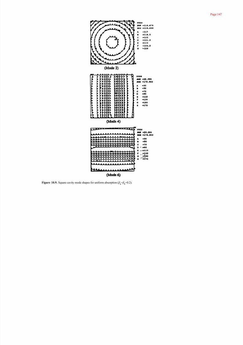
7/17/2019 The Boundary Element
http://slidepdf.com/reader/full/the-boundary-element 160/201
Page 147
Figure 10.9. Square cavity mode shapes for uniform absorption ( β a= β
b=0.2).

7/17/2019 The Boundary Element
http://slidepdf.com/reader/full/the-boundary-element 161/201
Page 148
Figure 10.10. Square cavity mode shapes for non-uniform absorption ( β a=0.9 and β
b=0).

7/17/2019 The Boundary Element
http://slidepdf.com/reader/full/the-boundary-element 162/201
Page 149
Chapter 11
Solution Methods of Eigenvalue Problems
11.1. Introduction
In Chapters 1 through 10, we have described in detail the boundary element discretization process and, specifically, the formulation of the boundary element eigenvalue problem encountered in elastodynamics, and acoustic fluid-structure analyses. Extraction of the eigenvalues and mode shapes from these eigenvalue problems, often, is
a computationally intensive process owing to the fact that most practical applications involve large matrices. Typical applications might be, finding the resonant
frequencies and mode shapes of mechanical systems like building structures, machinery parts, acoustic enclosures such as a concert hall, or acoustic fluid-structure
systems such as a submarine under water. Therefore, a computationally efficient eigenvalue extraction procedure is crucial to the success of the overall analysis
approach using the boundary element method (BEM).
The finite element based eigenvalue problems, usually, result in symmetric matrices. While the boundary element eigenvalue problem matrices are non-symmetric,
they represent only the boundary discretization and are smaller in size than the symmetric finite element matrices obtained by domain discretization. Therefore, an
efficient eigenvalue extraction procedure for the non-symmetric generalized eigenvalue problem would compliment the benefit gained by the smaller size boundary
element matrices.
11.2. Lanczos-based subspace approach
In most computational situations, we are interested in finding the lowest few eigenvalues and mode shapes of large matrices. This is true for practical structural dynamic
applications where the lowest and mid range resonant frequencies are of interest in the design of structural components and assemblies. The Lanczos method ofcomputing eigenvalues fits quite well for this situation, as the method has the ability to extract a few of the eigenvalues of large matrices, say 50 eigenvalues and mode
shapes of a large matrix of size 100,000 or more. In acoustic fluid-structure problems, it is often required to search for the resonant frequencies of the coupled system
in the lowest and the middle ranges of the frequency spectrum of the eigenproblem since the fluid domain resonant frequencies are closely spaced. The Lanczos
eigenvalue extraction method has been quite successfully employed in finite element based eigenvalue problems where the system matrices are symmetric. Since the
boundary eigenvalue problem matrices are non-symmetric, in this chapter we will show the Lanczos eigenvalue schemes designed specifically for such systems.

7/17/2019 The Boundary Element
http://slidepdf.com/reader/full/the-boundary-element 163/201
Page 150
Two widely used eigenvalue computational methods are the Subspace Iteration and the Lanczos Recursion methods. Both of these methods reduce a large
generalized eigenproblem shown below
into smaller-sized standard eigenproblem through orthogonal transformation into a subspace. The eigenvalues, μ j , j=1,2,…m of this transformed reduced size
eigenvalue problem
approximate the eigenvalues λ i of the original eigenvalue problem. These eigenvalues converge to that of the original problem as the subspace size m is progressively
increased.
Owing to the superior convergence properties, the Lanczos recursion method is quite widely employed in solving large eigenvalue problems arising in finite element
structural dynamic problems. Therefore, in this chapter the Lanczos recursion method will be presented for the solution of the boundary element eigenvalue problems.
11.3. Lanczos recursion method
The boundary element eigenvalue problems that we formulated in this book in Chapters 7 through 10 deal with non-symmetric generalized eigenvalue problems. The
eigenvalue problem presented in equation (8.22) is rewritten here for consideration.
where:
xi are the eigenvectors
λ i are the eigenvalues which represent the square of the resonant wave numbers k
i in acoustic problems
Matrices [A ] and [B] in the boundary element eigenvalue problem are non-symmetric. To solve a non-symmetric generalized eigenvalue problem, two possible
approaches can be used to transform the eigenproblem into a subspace. These are the Arnoldi's method, and the Lanczos method. Both of these methods are based on
the common origin of Krylov subspace techniques. In this book, however, the Lanczos algorithm will be described for the non-symmetric eigenvalue problem.
Solution of the non-symmetric eigenvalue problem using the Lanczos algorithm involves a two-sided recursion scheme applied to transform the generalized
eigenvalue problem given by equation (11.3) into a standard eigenvalue problem. In reference [192] detailed formulation of the Lanczos recursion is presented which
will be used here to concisely present the method. The two sets of Lanczos vectors generated by the recursion form the biorthogonal bases for the subspace ontowhich the generalized eigenproblem is projected to yield the standard eigenvalue problem. The matrix of the standard eigenvalue problem in the Krylov subspace results
in a tri-diagonal form lending itself for easy and efficient extraction of its eigenvalues μj. As the subspace size m is increased, μ j
converge to the eigenvalues λ i of the
original eigenproblem. In the limit when m=n,λi= μ
j.
(11.1)
(11.2)
(11.3)

7/17/2019 The Boundary Element
http://slidepdf.com/reader/full/the-boundary-element 164/201
Page 151
11.3.1. Lanczos recursion for the standard eigenvalue problem
In order to develop the Lanczos scheme for the generalized eigenvalue problem, the two-sided Lanczos recursion as applied to the following standard eigenvalue
problem will be reviewed briefly.
The two-sided recursion is applied to the matrix [A ] and its transpose [A ]T simultaneously as described in reference [192]. Starting from two arbitrarily chosen
vectors v1 and w
1 , two sets of Lanczos vectors v
j = v
1 , v
2 ,…v
m and w
j =w
1 , w
2 ,…w
m are generated from the right and left Krylov sequence of vectors. The
right and left Krylov sequence of vectors are given by
and
respectively. The set of m right and left Lanczos vectors v j and w
j form the biorthonormal bases for the subspace onto which the given matrix [A ] is projected. As
pointed out in references [192] and [193], a non-symmetric matrix [A ] has two sets of eigenvectors xi
and z i
which are the right and left eigenvectors belonging to
the original problem in equation (11.4) and the transposed eigenproblem
The eigenvector matrices [X ]=[ x1
, x2
,…, xn
] and [Z ]=[ z 1
, z 2
,…, z n
] will be biorthonormal yielding
where [I] is the identity matrix. The Lanczos scheme for the standard eigenvalue problem, therefore, is devised to generate two sets of vectors [V ]=[v1
, v2
,…, vm
]
and [W]=[w1
, w2
,…, wm
] from the right and left Krylov sequence such that
[V ] and [W] are biorthonormal. The two-sided Lanczos recursion used to generate the Lanczos vectors v j and w
j is given in references [178,192,193]. Here we
present the two-sided recursion for the standard eigenvalue problem [194] as an introduction to formulating the recursion scheme for the generalized eigenvalue
problem posed in equation (11.3).
For j=1, 2,…, m (m≤n) choose v
1 and w
1 such that w
1Tv
1=1.
When j=1, β 1
v0
=0, and δ1
w0
=0.
(11.4)
(11.5a)
(11.5b)
(11.6)
(11.7)
(11.8)
(11.9a)
(11.9b)
(11.10)
(11.11)
(11.12)
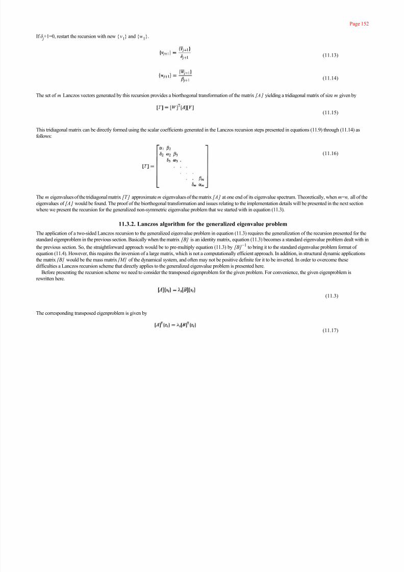
7/17/2019 The Boundary Element
http://slidepdf.com/reader/full/the-boundary-element 165/201
Page 152
If δ j+1=0, restart the recursion with new v
1 and w
1.
The set of m Lanczos vectors generated by this recursion provides a biorthogonal transformation of the matrix [A] yielding a tridiagonal matrix of size m given by
This tridiagonal matrix can be directly formed using the scalar coefficients generated in the Lanczos recursion steps presented in equations (11.9) through (11.14) as
follows:
The m eigenvalues of the tridiagonal matrix [T] approximatem eigenvalues of the matrix [A] at one end of its eigenvalue spectrum. Theoretically, when m=n, all of the
eigenvalues of [A] would be found. The proof of the biorthogonal transformation and issues relating to the implementation details will be presented in the next section
where we present the recursion for the generalized non-symmetric eigenvalue problem that we started with in equation (11.3).
11.3.2. Lanczos algorithm for the generalized eigenvalue problem
The application of a two-sided Lanczos recursion to the generalized eigenvalue problem in equation (11.3) requires the generalization of the recursion presented for the
standard eigenproblem in the previous section. Basically when the matrix [B] is an identity matrix, equation (11.3) becomes a standard eigenvalue problem dealt with in
the previous section. So, the straightforward approach would be to pre-multiply equation (11.3) by [B]−1 to bring it to the standard eigenvalue problem format of
equation (11.4). However, this requires the inversion of a large matrix, which is not a computationally efficient approach. In addition, in structural dynamic applications
the matrix [B] would be the mass matrix [M] of the dynamical system, and often may not be positive definite for it to be inverted. In order to overcome these
difficulties a Lanczos recursion scheme that directly applies to the generalized eigenvalue problem is presented here.
Before presenting the recursion scheme we need to consider the transposed eigenproblem for the given problem. For convenience, the given eigenproblem is
rewritten here.
The corresponding transposed eigenproblem is given by
(11.13)
(11.14)
(11.15)
(11.16)
(11.3)
(11.17)

7/17/2019 The Boundary Element
http://slidepdf.com/reader/full/the-boundary-element 166/201
Page 153
It can be shown that the eigenvalues of the transposed eigenproblem is the same as that of the original problem [178] owing to the biorthonormal property of the right-
and left-hand eigenvectors xi and z
i , respectively. The biorthonormality relationship is given by
Now we are ready to set up the Lanczos two-sided recursion for the generalized non-symmetric eigenproblem.
Two arbitrarily chosen vectors and normalizing the vectors as follows:
The right and left Krylov sequence of vectors that will map the right- and left-hand eigenvectors of the problem, respectively, are given by
Two sets of vectors [V]=[v1
, ν2
,…, vm
] and [W]=[w1
, w2
,…, wm
] are generated from the right and left Krylov sequence of vectors such that they satisfy the
biorthonormal relationship
Starting from equation (11.19) the right and left Lanczos vectors v j and w
j are generated employing the following steps.
For j=1, 2,…, m (m<n)
When j=1, β 1
v0
=0 and δ1
w0
=0.
If at any step during the recursion δ j+1=0, the recursion will have to be restarted with a new set of starting vectors v1 and w1.
(11.18)
(11.19)
(11.20a)
(11.20b)
(11.21)
(11.22)
(11.23)
(11.24)
(11.25)
(11.26)
(11.27)
(11.28)

7/17/2019 The Boundary Element
http://slidepdf.com/reader/full/the-boundary-element 167/201
Page 154
The coefficients α j,
β j and δ
j computed from the recursion presented in equations (11.19) and (11.22) through (11.28) are used to form the biorthogonally transformed
matrix [T] as shown in equation (11.16).
Since the eigenvalues are preserved under a biorthogonal transformation, the [T] matrix will contain the eigenvalues of the original problem (equation 11.3). A proof
of the transformation is shown here. In equation (11.3) let us set the right-hand eigenvector xi as
Then pre-multiplying by [W]T[B][A]−1 and after rearranging, equation (11.3) becomes
Using the biorthonormal property of the Lanczos vectors, namely [W]T[B][V]=[I], we can rewrite equation (11.30) as
where
and
Equation (11.31) is the transformed eigenvalue problem whose eigenvalues and eigenvectors are related to the original prolem through equations (11.33) and (11.29),
respectively. In a computer implementation of the Lanczos method the tridiagonal [T] matrix is directly formed using the scalar coefficients as given in equation (11.16).
A proof showing how equation (11.32) yields the same [T] matrix as in equation (11.16) can be found in the references [195] and [178] for symmetric and non-
symmetric eigenvalue problems, respectively. It is evident from the two sided recursion presented that when the system matrices are symmetric, [V]=[W] which leads
to a single sided recursion for the symmetric eigenvalue problems.
When the eigenvalues and eigenvectors of the [T] matrix are extracted, the eigenpairs of the original system can be recovered through equations (11.33) and
(11.29), respectively. In general the [T] matrix will be non-symmetric since β j=±δ
j , based on equation (11.26). A QR algorithm for non-symmetric matrices can be
employed to extract the eigenvalues μi of the tridiagonal [T] matrix quite efficiently. Complex arithmetic needs to be employed in the QR iterations since the
eigenvalues of a non-symmetric matrix can be complex.
The size of the [T] matrix will be equal to the number of pairs of Lanczos vectors m. We choose m much smaller than the size n of the original system. Therefore,
the eigenvalues μi (i=1, 2,…, m) of the [T] matrix will be an approximation to m eigenvalues λ
i of the original system. As the size of [T] matrix is increased, the μ
is
will converge to yield λ is that are close to the eigenvalues of the original problem. In practical implementations of the Lanczos scheme the number of Lanczos steps
taken is limited by issues relating to the loss of biorthogonality of the vectors. Measures that need to be taken to deal with the loss of biorthogonality of the Lanczos
vectors and the shift and search schemes are presented in the next section.
(11.29)
(11.30)
(11.31)
(11.32)
(11.33)

7/17/2019 The Boundary Element
http://slidepdf.com/reader/full/the-boundary-element 168/201
Page 155
11.3.3. Implementation details of the Lanczos scheme
Inverse of [A] and [A]T
As pointed out in the previous section, the matrix [A ] in the recursion is not explicitly inverted in practical implementations. Also, the inverse of [A ]T can be recovered
from the factorized [A ]. While the inverse of [A ]T is not explicitly computed, the product [A ]−T[B]Tw j in equation (11.23) is obtained using the triangularized [A ]
that is used to compute the product [A ]−1 [B] v j in equation (11.22). In order to illustrate the procedure we consider the first term on the right-hand sides of
equations (11.22) and (11.23).
Denoting the products [B] v j and [B]Tw
j by the vectors p and q, respectively, the equations (11.34a) and (11.34b) are rewritten as
The Gauss elimination process applied to the linear matrix equation (11.35a) involves reduction of the matrix [A ] into an upper triangular form and it can be symbolized
as follows:
L is a lower triangular matrix with unit diagonal elements. Its off-diagonal elements are composed of the multiplying factors used in the factorization of [A ] to get the
upper triangular matrix [S ]. The diagonal elements of [S ] are unity. [D] is a diagonal matrix containing the pivot coefficients that arise in the Gauss elimination process.
From equation (11.36) one can write the factored form of equation (11.35b) as follows:
For a symmetric [A ] it is easy to see that [L ]=[S ]T since [A ]T=[A ]. Owing to the non-symmetric [A], we have to store both [L ] and [S ]. Equations (11.36) and
(11.37) are now rewritten as
From equations (11.38), the solution vectors and ŵ can be computed through a simple back substitution process since [S ] and [L ]T are upper triangular
matrices. Therefore, by using the triangular matrices [L ] and [S] along with the pivot elements in [D], the matrix multiplication involving [A ]−1 and [A ]−T in equations
(11.22) and (11.23), respectively, can be computed in the two-sided recursion.
Reorthogonalization of Lanczos vectors
Loss of orthogonality of Lanczos vectors in finite precision computations is a deficiency of the recursion as presented in equations (11.22–11.28). Therefore,
application
(11.34a)
(11.34b)
(11.35a)
(11.35b)
(11.36)
(11.37)
(11.38a)
(11.38b)

7/17/2019 The Boundary Element
http://slidepdf.com/reader/full/the-boundary-element 169/201
Page 156
of a reorthogonalization step to the Lanczos vectors v j+1
and w j+1
obtained in equations (11.27) and (11.28) is an essential part of the recursion to maintain a
certain level of biorthogonality of the Lanczos vectors generated. Also, without any reorthogonalization an eigenvector that converges at the jth Lanczos step will
gradually grow into the Lanczos vectors computed in the subsequent steps of the recursion, causing an already converged eigenvalue to be detected again. Different
schemes of reorthogonalizing the current Lanczos vector against the already computed ones are presented in reference [195]. Either the full or the selective
reorthogonalization scheme can be used to maintain orthogonality between all the computed Lanczos vectors. In the literature the selective reorthogonalization scheme
has been shown to be economical in computations when the number of Lanczos step taken is large, say more than 50. However, in this presentation of the method a full
reorthogonalization scheme is shown which is tailored for the two-sided recursion where fewer than 50 or so Lanczos steps are taken. To ensure biorthogonality of the
pair of Lanczos vectors computed at the ( j+1)th step, the Gram-Schmidt coefficients are computed using the following expressions.
For i=1, 2,…, j
If any of the coefficients is, say θ k
and/or , is greater than a predetermined small number ε0
, then v j+1
and w j+1
are modified using the following Gram-Schmidt
biorthogonalization steps:
The value of the biorthogonality tolerance ε0
is chosen based on the machine round-off error. While the level of biorthogonality of Lanczos vectors is dependent upon
the tolerance ε0
, it also affects the ability of the recursion to capture the repeated eigenvalues if any are present in a problem. Therefore the choice of the value of ε0
should be done with care. A value of 10−8 has been found to work well based on the above two requirements on the tolerance value. The number of steps it takes to
capture a repeated mode is problem dependent. In the numerical studies conducted with acoustic fluid-structure eigenvalue problems, a repeated mode usually
converged in about five to ten Lanczos steps after the first has converged. However, eigenvalues that are complex always converged in complex conjugate pairs. In
reference [196] Kim and Craig use a block Lanczos algorithm in order to capture the repeated eigenvalues. By choosing a block size equal to or larger than the
multiplicity of the eigenvalues, the repeated modes are found more reliably.
Eigenvalue search strategy using shift logic
In the two-sided recursion applied to the standard eigenvalue problem, equation (11.4), the Lanczos scheme has the property of quickly converging to the largest
eigenvalues of the matrix [A ]. Owing to the transformation that takes place in the generalized eigenproblem recursion, which involves [A ]−1 , the lowest eigenvalues
converge first as can be seen from the relationship μi=1/λ
i in equation (11.33).
(11.39a)
(11.39b)
(11.40a)
(11.40b)

7/17/2019 The Boundary Element
http://slidepdf.com/reader/full/the-boundary-element 170/201
Page 157
The convergence of eigenvalues in a specified part of the eigenvalue spectrum can be accelerated by applying an appropriate shift to the given eigenproblem. A
spectral transformation of equation (11.3) is introduced by setting
The spectral transformed eigenvalue problem is then given by
In the non-symmetric eigenvalue problem with complex eigenvalues, this transformation accelerates convergence of eigenvalues whose magnitude is close to that of the
shift σ . Through numerical experimentation it has been observed that the shift needs to be only a real number even when complex eigenvalues are expected. The value
of σ is chosen close to the magnitude of the complex eigenvalues searched.
The following approach is used to search for the eigenvalues in a specified part of the eigenvalue spectrum. A shift σ equal to the lowest eigenvalue magnitude sought
is applied to the problem. If the number of eigenvalues requested is r, m=r + s recursion steps are performed. The value of s is chosen such that r eigenvalues with
magnitude beyond the shift would converge without missing any modes. After each Lanczos recursion step, the eigenvalues are computed and the converged ones
accumulated. At the end of m steps, the first r eigenvalues with magnitude higher than the shift, arranged in ascending order of their magnitude, are presented as
converged eigenvalues. After some numerical experimentation a value of s=16 was chosen. However, to ensure that no eigenvalues are missed a Sturm sequence
check, as presented in reference [186], should be employed combined with the strategy outlined. For the non-symmetric eigenproblems, however, a Sturm sequence
check procedure is unavailable to the knowledge of the authors of this book.
11.4. Example problems
We present two example problems as a demonstration of the working of the two-sided Lanczos recursion presented. The first one is a generalized eigenproblem of
12×12 matrices [A ] and [B] with known eigenvalues that are complex. The second example is an acoustic fluid-structure problem where we are interested in finding
the eigenvalues of a fluid filled cylindrical shell for which the theoretical resonant frequencies are available for comparison.
Example 11.1: Eigenvalues of a non-symmetric matrix
In this example the [A ] and [B] matrices of the generalized eigenproblem were generated from two 12×12 matrices where one is a block-diagonal matrix of block size
2 and the second one is an identity matrix. The 2×2 blocks of the block-diagonal matrix was filled with the real and imaginary parts of the complex conjugate eigenvalue
pair chosen a priori. The diagonals of a 2×2 block are filled with the real part of a complex eigenvalue and the off-diagonals with the imaginary part forming a skew
symmetric matrix. The matrices [A ] and [B] were obtained from the first and the second matrices, respectively, by pre-multiplying them with an arbitrarily chosen
matrix filled with random numbers. So, the eigenvalues of the generalized eigenvalue problem is known beforehand for comparing with the computed eigenvalues
employing the Lanczos
(11.41)
(11.42)

7/17/2019 The Boundary Element
http://slidepdf.com/reader/full/the-boundary-element 171/201
Page 158
two-sided recursion presented in the previous section. The matrices [A ] and [B] are shown in Table 11.1.
This generalized eigenproblem has both real and complex eigenvalues. The computed and known eigenvalues are presented in Table 11.2. Since the problem
considered here is quite small, the Lanczos recursion was performed to the full size of the system ( m=n=l2), transforming [A ] and [B] into a subspace size of 12
yielding a 12×12 [T ] matrix. It is seen from the table of results that the eigenvalues of the non-symmetric generalized eigenproblem are quite accurately computed bythe Lanczos method presented. In general for large eigenvalue problems the number of Lanczos steps taken can be much smaller than the size of the matrices [A ] and
[B] in order to extract the first few eigenvalues of the problem. The next example is designed to illustrate this point.
Example 11.2: Fluid-structure eigenvalue problem
This example is an illustration of a practical application of the non-symmetric generalized eigenvalue solution method presented in the previous section. The problem
considered is an acoustic fluid-structure interaction problem. The eigenvalues of this problem will all be real values even though the stiffness and mass matrices of the
problem, [K ] and [M], respectively, are non-symmetric. A cylindrical shell of circular cross section filled with fluid is analyzed employing the Finite Element method
(FEM). The length of the shell is assumed to be infinite. Shown in Figure 11.1 is the cross section
Table 11.1. Matrices [A] and [B] used in Example 11.1.
[A] Matrix
−41 176 393 42 14 616 −700 −1270 5333 2376 8320 −1400
34 418 477 225 14 378 1685 −315 −455 5199 −11960 5200
−4 −924 −396 354 −315 574 590 660 3191 −54 6760 −6000
−11 −330 180 −555 −280 182 90 1550 −3712 −5844 3120 30000
19 −836 273 21 112 −238 −70 400 −968 −826 −1560 76000
3 44 75 −159 217 518 −370 −1310 −2273 5722 8320 −98000
11 1056 −648 −399 56 462 −375 625 5493 −164 10140 8000
34 286 −300 −537 −301 −644 −815 −285 2125 4724 −8840 −12000
−49 −748 −576 93 −21 336 900 540 6256 −2156 9620 96000
−3 594 −39 48 −273 154 −280 920 1436 1493 10660 90000
−17 110 261 −690 91 −140 −210 1200 −2629 3277 11180 −24000
29 −44 −69 642 −203 350 −555 −1285 4944 2479 5720 −36000
[B] Matrix
−410 16 90 33 2 88 125 −215 −16 43 64 7
340 38 99 81 2 54 195 220 −41 −1 −92 −26
−40 −84 −114 60 −45 82 −45 145 2 25 52 3
−110 −30 75 −120 −40 26 −220 150 44 −32 24 −15190 −76 63 21 16 −34 −65 25 6 −8 −12 −38
30 4 27 −33 31 74 160 −170 −46 −15 64 49
110 96 −129 −132 8 66 −125 0 4 43 78 −4
340 26 −39 −144 43 −92 −30 −145 −36 19 −68 6
−490 −68 −141 −12 −3 48 0 180 20 48 74 −48
−30 54 −12 9 −39 22 −160 40 −11 12 82 −45
−170 10 102 −147 13 −20 −195 75 −27 −19 86 12
290 −4 −54 147 −29 50 140 −195 −17 40 44 18

7/17/2019 The Boundary Element
http://slidepdf.com/reader/full/the-boundary-element 172/201
Page 159
Figure 11.1. Fluid-filled Shell model and mode shapes (Shell: wall thickness t =0.102 m, Young’s modulus E =2.068e11 N/m2, Poisson’s
ratio v=0, density ρ s
=2403 kg/m3
; fluid: bulk modulus K =2.25e9 N/m2, density ρ=1000 kg/m3
; modes 2, 4, 6, 8, 10 have the
same shape but are oriented at 90 degrees to modes 1, 3, 5, 7, 9 respectively).
Table 11.2. Eigenvalues of the input matrix problem in example 11.1.
No. Known eigenvalues Computed eigenvalues
1 0.1 0.100000 +0.000000J
2 4−1J 4.000000 −1.000000J
3 4+1J 4.000000 +1.000000J
4 3−5J 3.000000 −5.000000J
5 3+5J 3.000000 +5.000000J
6 7 7.000000 −0.000000J
7 7 7.000000 +0.000000J
8 11 11.000000 +0.000000J
9 8−127J 8.000000 −127.000000J
10 8+127J 8.000000 +127.000000J
11 130 129.99989 +0.000000J
12 −2000 −2000.022577 +0.000000J

7/17/2019 The Boundary Element
http://slidepdf.com/reader/full/the-boundary-element 173/201
Page 160
of the finite element discretized shell and the fluid inside. The material properties of the steel shell and the water inside are shown in the figure.
In Section 10.2.1 the same problem was considered to show the application of the boundary element eigenvalue problem formulation developed in Chapters 7
through 10. In this current chapter, however, it is used to demonstrate application of the non-symmetric eigenvalue solver.
Employing the FEM, the dynamic matrix equation for free vibration analysis of an acoustic fluid-structure interaction problem is shown below in equation (11.44).
The shell element and the acoustic fluid element available in the ANSYS® general-purpose finite element program [160] are used. The shell element is a four-node
element allowing cubic variation of the radial displacement along circumference and constant displacement through the thickness. The acoustic element is a eight-node
three-dimensional (3-D) brick with tri-linear pressure shape functions representing the acoustic wave equation (5.1). Even though 3-D elements are used, the analysis is
carried out in 2-D to treat the planar cylindrical ring problem. The free vibration response equation of the coupled problem is rewritten from Chapter 10 here. The
structural dynamic equation (10.4) is combined with the following fluid finite element matrix equation from Zienkiewicz and Newton [186]
to form the fluid-structure matrix equation given by
U and P contain the unknown nodal displacements and pressures respectively. [K s ] and [M
s ] are the stiffness and mass matrices of the shell. ρ[RT ] is the matrix
generated at the fluid-shell interface using the interface condition given by equation (10.1), namely the fluid pressure gradient at the interface balances the acceleration
force exerted by the structure. ρ is the density of the fluid. [K f ] and [M
f ] are the fluid “stiffness” and “mass” matrices, respectively. This is a non-symmetric matrix
generalized eigenproblem even though the sub-matrices are symmetric except for the coupling submatrix [R]. The two-sided Lanczos recursion was applied to this
eigenvalue problem to extract the eigenvalues .
The first ten non-zero frequencies,i=ω
i/2π, extracted are presented in Table 11.3. Due to the geometric symmetry of the problem the eigenvalues appear in pairs
which correspond to the two eigenmodes oriented about two orthogonal diameters of the ring. The five mode shapes computed are also shown in Figure 11.1. The first
two pairs of eigenvalues are in good agreement with the theoretical solution presented by Yu [188]. At higher modes the computed frequencies slightly differ from the
theoretical frequencies which may be attributed to the Finite Element discretization approximation of the continuum.
11.5. Summary statements on the non-symmetric Lanczos eigensolver
The Lanczos two-sided algorithm presented in Sections 11.2 through 11.4 is given in its most general form. Therefore it can be applied to extract both the real and
(11.43)
(11.44)

7/17/2019 The Boundary Element
http://slidepdf.com/reader/full/the-boundary-element 174/201
Page 161
complex eigenvalues of a non-symmetric system. For the Boundary Element algebraic eigenvalue problem this method is ideally suited owing to its generality of the
formulation to handle non-symmetric matrices with the possibility of complex eigenvalues that may arise due to discretization approximation of the continuum.
For short Lanczos runs where only a few eigenvalues of a large problem are sought, the computation speed was found to be quite fast compared to other subspace
procedures. When a large number of Lanczos steps are taken in order to compute several eigenvalues, say more than 100 modes, a selective reorthogonalization
procedure will help improve the computational performance of the method.
11.6. Damped system eigenvalue problem solution
In Section 10.3 we described the inclusion of sound absorption in acoustic boundary element eigenvalue formulations. Also, in structural dynamic applications involving
damped systems a damping matrix would arise in the eigenvalue formulations leading to a quadratic eigenvalue problem presented in equation (10.22). This quadratic
eigenvalue problem equation is rewritten here.
In dynamic applications, [A] and [B] represent the stiffness and mass matrices, respectively. The matrix [C] is the damping matrix, which accounts for the dissipation
of energy. When [C] is zero, equation (11.45) reduces to the generalized eigenvalue problem for which the Lanczos recursion was presented in Section 11.3. In the
damped system boundary element eigenvalue problem these matrices are non-symmetric and in practical situations their size n can be large. As we showed in the
previous sections, the Lanczos subspace approach would be best suited for such systems where only a few eigenvalues at one end of the spectrum, usually the lowestones, are of interest.
One of the straightforward approaches is to employ the method of matrix augmentation which leads to a linear eigenvalue problem of the form in equation (11.3).
Then the Lanczos two-sided recursion presented in Section 11.3 can be employed to solve
Table 11.3. Eigenfrequencies of the fluid-filled shell.
Frequency (Hz)
Mode Theoretical Computed
1 25.038 25.025378
2 25.038 25.025378
3 77.924 78.380262
4 77.924 78.380263
5 160.42 162.55957
6 160.42 162.55959
7 272.99 278.84044
8 272.99 278.84045
9 415.17 427.61895
10 415.17 427.61924
(11.45)

7/17/2019 The Boundary Element
http://slidepdf.com/reader/full/the-boundary-element 175/201
Page 162
for the eigenvalues and vectors of the problem. Defining a new vector , we can write a null equation.
Combining it with equation (11.45), the augmented linear eigenproblem given below can be arrived at.
Solution of this linear eigenproblem involves matrices that are doubled in size to 2 n and requires double the computational effort. Therefore, in the sections that follow
the two-sided Lanczos recursion that applies directly to non-symmetric quadratic eigenvalue problem given by equation (11.45) is developed.
11.7. Lanczos two-sided recursion for the quadratic eigenvalue problem
Pursuing along the same lines of Section 11.3 the Lanczos two-sided recursion scheme to compute the eigenvalues of the quadratic eigenvalue problem is shown in this
section. In the development of the algorithm we will make use of the biorthonormal transformation of the quadratic eigenproblem that leads to the tridiagonal subspace
matrix [eqn. (11.16)]. As we saw in Section 11.3, the two-sided recursion is developed by considering the original eigenproblem and its transpose in order to generate
two sets of vectors namely the right and left hand Lanczos vectors. The transposed quadratic eigenvalue problem is written below.
Basically, the zeroes of the determinant equation
are the eigenvalues λ i , of equation (11.48). Since the determinant of a matrix is the same as that of its transpose, it is clear that the eigenvalues of the original and the
transposed problems, given by equations (11.45) and (11.48), respectively are the same. The associated eigenvectors xi and z
i are the right- and left-hand
eigenvectors. Therefore, the Lanczos recursion is derived considering the original eigenproblem in equation (11.45) and its transposed problem in equation (11.48) in
order to biorthogonally transform the n order quadratic problem into a standard eigenvalue problem (equation 11.31) of order m, m<n, in the subspace of the Lanczos
vectors.
11.7.1. Biorthogonality relationship for the quadratic eigenvalue problem
The biorthogonality relationship of the right and left hand eigenvectors can be derived by considering two distinct eigenvalues λ i and λ
j , i≠ j, in equations (11.45) and
(11.48), respectively. Corresponding to the eigenvalue λ j , equation (11.48) is written as
Pre-multiplying equation (1 1.45) by z j T and equation (1 1.50) by x
i T and transposing it, the difference between the two resulting equations is written down below.
(11.46)
(11.47)
(11.48)
(11.49)
(11.50)
(11.51)

7/17/2019 The Boundary Element
http://slidepdf.com/reader/full/the-boundary-element 176/201
Page 163
Factoring out (λ i−
λ j
) in equation (11.51), and noting that λ i≠λ
j , the biorthogonality relationship is found to be
Here, we introduce two additional eigenvectors as we did to arrive at the linearized eigenproblem in equation (11.47).
Equation (11.52) can now be written as
The generalized biorthogonality condition for the quadratic eigenproblem, therefore, is given by equation (11.54). When j=i, if the eigenvectors are normalized such that
The generalized biorthonormal condition of the quadratic eigenproblem is written down as follows:
Normalization given by equation (11.55) may not always be possible due to the possibility that the sum of the three scalar products may yield a null value. In equation
(11.56), [X ]=[ x1 ,x
2 ,…,x
n ] and [Z ]=[z
1 , z
2 ,…, z
n ] are the right- and left-hand eigenvector matrices. For a given eigenvalue λ
i , the eigenvectors defined in equation
(11.53) are obtainable from xi and z
i . Therefore, are called the right- and left-hand dependent eigenvector matrices of the quadratic
eigenproblem. From the biorthonormal relationship established here it is evident that the Lanczos recursion for the quadratic eigenproblem will need to generate two
independent and two dependent sets of right- and left-hand vectors in order to biorthogonally transform the eigenproblem.
11.7.2. Lanczos recursion
With the definition of the biorthonormality expressions given by equation (11.56) we are ready to develop the Lanczos recursion scheme for the non-symmetric
quadratic eigenvalue problem posed in equations (11.45) and (11.48) earlier in this section. The Lanczos recursion for this case is developed in detail with complete
proofs and derivations by Rajakumar [179]. Here we will present the algorithm from the point of view of practical implementation of the recursion, without delving into
to detailed derivations.
Again, along the lines of Section 11.3.2, we start by seeking the Krylov sequence of vectors that will generate the Lanczos vectors. The eigenproblem equations
(11.45) and (11.48) can be rewritten using the definition of the dependent eigenvectors in equation (11.53) as follows:
(11.52)
(11.53a)
(11.53b)
(11.54)
(11.55)
(11.56)
(11.57a)
(11.57b)

7/17/2019 The Boundary Element
http://slidepdf.com/reader/full/the-boundary-element 177/201
Page 164
Now, two sets of arbitrarily chosen vectors ( , ŝ 1
) are used to start the two pairs of Krylov sequence of vectors that apply to equations (11.45) and (11.48).
From equations (11.57), the right- and left-hand sequence of vectors that will map the independent eigenvectors xi and z
i , respectively, are
From equations (11.53), the right- and left-hand sequences that will map the dependent eigenvectors , respectively, can be written as
Inspecting equations (11.58) and (11.59), we can see that the primary Krylov sequences are coupled to the secondary sequences. These above Krylov sequences can
also be written down by looking at the linearized augmented form of the quadratic eigenproblem given in equation (11.47). Now we are ready to proceed to present
the Lanczos recursion for the problem.
Two sets of vectors . Then the recursion steps are for j=1, 2,…, m (m≤n),
(when j=1, β 1
ν0
= β 1
r 0
=δ1
w0
=δ1
s0
=0)
(11.58a)
(11.58b)
(11.59a)
(11.59b)
(11.60a)
(11.60b)
(11.61a)
(11.61b)
(11.62)
(11.63)
(11.64)
(11.65)
(11.66a)
(11.66b)

7/17/2019 The Boundary Element
http://slidepdf.com/reader/full/the-boundary-element 178/201
Page 165
The recursion scheme presented above in equations (11.60) through (11.66) generates an extra set of right- and left-hand Lanczos vectors as compared to the linear
non-symmetric generalized eigenvalue problem shown in Section 11.3. The Lanczos vectors generated in the recursion scheme presented above satisfy the generalized
biorthonormality condition given by
The coefficients generated in the recursion α j , β
j , β
j , and δ
j are used to form the tridiagonal matrix [T ] as shown in equation (11.16) whose eigenvalues approximate the
eigenvalues of the quadratic eigenproblem in equation (11.45). So, the quadratic eigenproblem reduces to solving the following standard eigenproblem
in the Lanczos vectors subspace of size m. The eigenvalues and eigenvectors of [T ] matrix and those of the original quadratic eigenproblem are related by μi=1/λ
i and
yi=[V]xi. As the subspace size m is progressively increased, the eigenvalues of equation (11.68) converge to yield the eigenvalues λ i of the quadratic eigenvalue
problem. Theoretically, when m=2n all of the eigenvalues of the quadratic eigenproblem will be extracted. However, often in practical applications involving large
matrices only the first few eigenvalues are of interest which will converge in a few Lanczos recursion steps m«2n. Spectral transformation of the eigenproblem to
improve convergence of the eigenvalue in a specified part of the eigenvalue spectrum is presented in the next section dealing with practical implementation details.
11.7.3. Implementation details of quadratic Lanczos scheme
Proof of biorthogonal transformation
First we present the biorthogonal transformation proof that leads to the tridiagonal matrix [T ] for the quadratic Lanczos recursion scheme. The right hand
eigenvectors are projected onto the subspace spanned by the Lanczos vectors as follows:
Substituting equation (11.69) into (11.53a) and (11.57a), we multiply (11.57a) by ([W]T[C ]+[S]T [B])[A]−1 and (11.53a) by [W]T[B], and add the two equations
to get
Since the Lanczos vectors are biorthonormal, satisfying equation (11.67), we obtain the tridiagonal subspace eigenproblem
where [T ] is the subspace matrix given by
Equation (11.71), which is the same as shown in (11.68), is the biorthogonally transformed eigenproblem whose eigenvectors relate to the original eigenproblem
through (11.69). In the Lanczos eigenvalue solution process the [T ] matrix is directly formed using the coefficients generated in the recursion steps in equations (11.62)
through
(11.67)
(11.68)
(11.69)
(11.70)
(11.71)
(11.72)

7/17/2019 The Boundary Element
http://slidepdf.com/reader/full/the-boundary-element 179/201
Page 166
(11.65). The proof showing that equation (11.72), in fact, results in a tridiagonal matrix (11.16) is given in reference [163].
Spectral transformation
In computer implementation of the algorithm, to accelerate convergence of the eigenvalues in a specified eigenvalue magnitude spectrum, a spectral transformation
needs to be incorporated. A shift of the eigenvalues is introduced as shown here.
Substituting equation (11.73) into (11.45) leads to the spectrally transformed eigenproblem given by
where [Aσ ]=([A ]+σ[C]+σ 2[B]) and [C
σ ]=([C ]+2σ[B]). The Lanczos algorithm has the property of converging first to the largest magnitude eigenvalues in the
spectrum. Therefore, in view of the eigenvalue transformation equation, μi=1/λ
i, the lowest magnitude eigenvalues of the quadratic eigenvalue problem will converge
first. The use of a real valued shift σ accelerates convergence of the eigenvalues that are close to its magnitude. Also, the shifting is needed to extract the rigid body
modes in structural dynamic applications.
Re-biorthogonalization of Lanczos vectors
Equations (11.60) and (11.61) are the biorthogonalization steps of the recursion, where the set of ( j+1)st vectors are biorthogonalized against the jth and ( j−1)st
vectors. These two steps are responsible for maintaining biorthogonality of Lanczos vectors such that the biorthogonality equation (11.67) is satisfied. However, as
pointed out in Section 11.3.3 for the generalized non-symmetric eigenproblem, the Lanczos vectors gradually loose biorthogonality as the recursions proceed incomputer implementations. This loss of biorthogonality occurs due to the limitation of the finite precision calculations that the computers employ. In exact arithmetic the
recursion scheme as presented produces biorthonormal vectors. In other words, if the computers were to handle arithmetic calculations in infinite precision, i.e., in exact
arithmetic, the Lanczos vectors as generated will be biorthonormal. Due to this practical limitation, a re-biorthogonal scheme to restore biorthogonality of the vectors is
necessary.
The ( j+1)st vectors computed in equations (11.66) are checked for their of level of biorthogonality with respect to all of the previous vectors that have been
generated. For i=1,2,..., j, the biorthogonality coefficients are calculated as follows:
If the magnitude of any of the coefficients, say, the k th coefficient, exceeds a predetermined small value ε0 , then the vectors are biorthogonalized with respect to the k th
set of Lanczos vectors.
(11.73)
(11.74)
(11.75a)
(11.75b)
(11.76a)
(11.76b)

7/17/2019 The Boundary Element
http://slidepdf.com/reader/full/the-boundary-element 180/201
Page 167
The value of ε0
is dependent on the machine precision of the computer employed. Usually, a value of 10−8 has been found to work well. A much smaller value of ε0
will
yield Lanczos vectors with a higher level of biorthogonality. However, the algorithm also depends on the finite precision of the machine to capture repeated eigenvalues
that may be present in a problem, as described in reference [195]. Therefore, the value of ε0
should be chosen at least slightly higher than the machine precision in order
for the repeated eigenvalues to converge. The value of ε0
=10−8 is based on the numerical experimentation such that a repeated eigenvalue converged within five to ten
recursion steps after the first has converged. When there are complex eigenvalues in a problem, they converged in conjugate pairs.
Eigenvalue search strategy
The eigenvalues in a specified magnitude range are searched by introducing a shift σ equal to the lower limit of the eigenvalue magnitudes sought. The search procedure
employed for the quadratic eigenproblem here is exactly same as that used for the non-symmetric generalized eigenproblem described in Section 11.3.3. In thequadratic eigenproblem, however occasional break down of the recursion may occur due to the possibility of the sum of the scalar products resulting in a null value for
the normalization coefficient Δ j+1
computed in equation (11.63). As can be seen in equations (11.64) through (11.66), this will result in a non-definable ( j+1)st
Lanczos vectors. In this event the remedy is to restart the recursion, after saving the converged eigenvalues, with a new set of starting vectors. This occurrence is,
however, rare. If |Δ j+1
| drops close to zero, there are two possibilities: (a) the aforementioned breakdown has occurred, and (b) the eigenvalues have all converged in
the range of |σ |<|λ i|<|λ k |, for k<j, and the magnitude of the next eigenvalue, λ
k +1, is much highe than that of λ
k , often by more than two orders of magnitude. Under
such conditions, the best approach is to restart the recursion employing a new shift of magnitude slightly lower than that of the largest converged eigenvalue in the
terminated recursion.
11.7.4. Quadratic eigenvalue problem examples
Two examples are presented here to demonstrate the application of the Lanczos recursion for quadratic eigenvalue problems. First one is an input matrix problem
where three randomly generated matrices from known eigenvalues form the [A], [B] and [C ] matrices of the quadratic eigenvalue problem. The second one is a
simply supported beam modeled using the FEM with damping specified to absorb energy. For additional examples showing the application of the method to Boundary
Element eigenvalue problem the reader is directed to Chapter 10, examples 4, 5, and 6 where acoustic cavity eigenvalue problems have been considered.
Example 11.3
This is a small size (6×6) input matrix problem showing the validation of the Lanczos recursion scheme for the quadratic eigenvalue problem. The matrices [A], [C],
and [B] are generated from a set of known complex eigenvalues λ i=σ
t −jω
i , λ
i+1=σ
i+jω
i where are given by λ
i=σ
i ± jω
i. Then
the diagonal matrices are pre-multiplied by an arbitrary

7/17/2019 The Boundary Element
http://slidepdf.com/reader/full/the-boundary-element 181/201
Page 168
matrix [E ] of size 6×6 whose elements are randomly filled. The quadratic eigenproblem formed by the product matrices [A ]=[E][Ad ], [C]=[E][C
d ],[B ]=[E][B
d ]
have the same eigenpairs as that of the diagonal quadratic eigenvalue problem. The input matrices generated by this process are given in Table 11.4.
The computed eigenvalues of this quadratic eigenvalue problem are listed in Table 11.5 along with the known eigenvalues of problem. As we know, the eigenvaluesof the quadratic eigenproblem appear in complex conjugate pairs. For the 6×6
Table 11.4. Input matrices of Example 11.3.
[A] Matrix
324 −2190 23160 10864415 −4182340 109027740
72 −2482 −1930 4205580 13383488 −7268516
1152 657 13510 −8411160 14219956 32708322
612 1314 −13510 −2803720 12547020 85405063
900 −2409 −52110 18224180 −11710552 61782386
1728 −2263 88780 −2102790 3764106 −47245354
[C] Matrix
−108 180 −216 −62 −940 161760
24 204 18 −24 3008 −10784
−384 −54 −126 48 3196 48528
−204 −108 126 16 2820 126712
−300 198 486 −104 −2632 91664
−576 186 −828 12 846 −70096
[B] Matrix
9 −30 12 31 −10 60
2 −34 −1 12 32 −4
32 9 7 −24 34 1817 18 −7 −8 30 47
25 −33 −27 52 −28 34
48 −31 46 −6 9 −26
Table 11.5. Eigenvalues of Example 11.3.
Eigenvalues
No. Known Computed
1 6+0J 6.0004588 0.99258436E−06J
2 6−0J 5.9995408 −0.989798 12E−06J
3 3+8J 2.9999997 8.0000007J
4 3−8J 2.9999997 −8.0000007J
5 9+43J 9.0000022 42.999999J
6 9−43J 9.0000022 −42.999998J
7 1+592J 1.0000667 591.99991J
8 1–592J 1.0000655 −591.99991J
9 −47+645J −46.999961 644.99963J
10 −47−645 J −46.999959 −644.99963J
11 −1348+5J −1348.0007 5.0045941J
12 −1348−5J −1348.0007 −5.0045945J

7/17/2019 The Boundary Element
http://slidepdf.com/reader/full/the-boundary-element 182/201
Page 169
Figure 11.2. Simply supported beam of square cross section (Young’s modulus E =12E10, density ρ=1E4, area A=1, moment of inertia I =1/12, proportional damping coefficients: α=0.12, β=0.003). (a) Simply supported beam; (b) Finite element discretization.
system all of the 6 conjugate pairs of eigenvalues were computed by taking m=12 Lanczos steps. In spite of the wide spread of the eigenvalue magnitude spectrum, the
eigenvalues converged and are in good agreement with the actual eigenvalues of the problem.
Example 11.4
A simply supported beam of square cross section, shown in Figure 11.2, is discretized by finite elements to compute its damped system resonant frequencies. The
damping matrix that accounts for the dissipation of energy is formed by considering proportional damping expression given by [C ]=α[M]+ β[K ]. Here, α and β are the
scalar coefficients that bring a fraction of the mass and stiffness matrices, [K ] and [M], respectively, of the beam into [C ]. The resulting quadratic eigenvalue problemof the beam is given by
The beam was divided into 50 finite elements along its length employing the ANSYS® program and the damped system frequencies computed using the Lanczos
recursion scheme. The computed eigenvalues of the damped system eigenproblem are presented in Table 11.6. The eigenfrequencies of the beam are given by the
following analytical expression [197].
where λ n
are the circular eigenfrequencies of the beam. The material properties of the beam, Young’s modulus and the density, are shown in Figure 11.2. The cross
section area and moment of inertia are given by A and I, respectively. In Table 11.6 the first ten frequencies computed are listed along with the analytical frequencies.
The agreement of the computed values with the analytical frequencies is quite good. The
(11.77)
(11.78)

7/17/2019 The Boundary Element
http://slidepdf.com/reader/full/the-boundary-element 183/201
Page 170
slight differences are partly attributable to the discretization error inherent in the finite element discretization of the continuum.
11.8. Summary statements on eigenvalue computation algorithms
In this chapter we presented the tools needed to efficiently solve the boundary element eigenvalue problems. It turns out that the algebraic eigenvalue problemsdeveloped in Chapters 7 through 10 can all be handled using one of the Lanczos computational schemes presented in this chapter. In the literature, in addition to the
Lanczos two-sided recursion schemes, the Arnoldi’s method is found to be used for non-symmetric eigenvalue problems. While the two methods share the common
Krylov sequence of vectors, they differ in the resulting subspace matrix. The Lanczos two-sided recursion is attractive due to the fact that the resulting subspace matrix
is tridiagonal whose eigenvalues can be extracted quite efficiently. Furthermore, the Lanczos algorithm has been quite widely employed in commercial finite element
software for the symmetric problem, and thus the incorporation of the non-symmetric schemes would involve extension of the implementations to the non-symmetric
problem.
In addition, symmetric boundary element formulations have been actively pursued to make the method more attractive for large practical problems. The Lanczos
schemes developed in this chapter can be quite easily specialized for symmetric eigenproblems.
Table 11.6. Eigenfrequencies of the beam with proportional damping.
Frequency (Hz)
Mode Analytical Computed
1 −0.38258801E−01 +1.7449094J −0.38231453E−01 +1.7440785J
2 −0.38258801E−01 −1.7449094J −0.38231453E−01 −1.7440785J
3 −0.46890141 +6.9655503J −0.46721040 +6.9527743J
4 −0.46890141 −6.9655503J −0.46721040 −6.9527743J
5 −2.3350194 +15.533437J −2.3159626 +15.471081J
6 −2.3350194 −15.533437 J −2.3159626 −15.471081J
7 −7.3591831 +26.938125J −7.2530238 +26.757246J
8 −7.3591831 −26.938125J −7.2530238 −26.757246J
9 −17.952991 +39.768680J −17.551764 +39.410940J
10 −17.952991 −39.768680J −17.551764 −39.410940J

7/17/2019 The Boundary Element
http://slidepdf.com/reader/full/the-boundary-element 184/201
Page 171
Chapter 12
Discussion and Future Research
12.1. Discussion on boundary element eigenvalue methodologies
The evolutionary history of the development of eigenvalue formulations, based on the boundary element method (BEM), is presented in this book. The material is presented in a chronologically organized manner, starting from the early Determinant Search Method (DSM) to the most recently proposed techniques such as the
Multiple Reciprocity Method (MRM), Series Expansion Method (SEM), etc. An alternative approach would have been to organize the materials based upon the fields
of application such as two-dimensional (2-D) elasticity, three-dimensional (3-D) elasticity, plates and shells, 2-D acoustics and so on. This would, however, have
turned us away from our stated goal to focus our attention on the development of eigenvalue formulation itself. We chose the chronological approach over the
application-driven approach because the BEM based eigenvalue formulations are still in an evolving stage and more research will be required in a number of related
areas to improve the degree of maturity of the technique. The book will hopefully encourage researchers to continue work on the subject.
We have reviewed and provided detailed eigenvalue formulations for acoustics, elasticity and plate vibrations. All the formulations, proposed so far in the literature to
solve BE eigenvalue problems such as Determinant Search Method, enhanced Determinant Search Method, Internal Cell Method (ICM), Dual Reciprocity Method
(DRM), Particular Integral Method (PIM) and its variation, Multiple Reciprocity Method (MRM), Series Expansion Method (SEM) with matrix augmentation and so
on, are discussed in the book. Wherever appropriate, the advantages and disadvantages of each method are also recorded in the relevant chapters. In the next section
we will briefly compare BE eigenvalue formulations with finite element (FE) eigenvalue formulation. A few topics related to BE eigenvalue formulations are not covered
in the book. These topics are enumerated in Section 12.3. The final section is dedicated to the discussion of possible future research that can be undertaken in order to
improve the performance of BE eigensolution methodology and to extend its capability.
The book is written such that a beginner on the subject of BEM can learn the basics of the method and then gradually get into the discussion of eigenvalue
formulations. The basics of BEM are developed using simple potential problems to make it easier for the reader to enter into the BEM subject matter without difficulty.All the important details of basic BE formulation are worked out in Chapters 2 through 4. A sufficient number of example problems are also presented in these chapters
in order to demonstrate the application of the BE formulations developed there.

7/17/2019 The Boundary Element
http://slidepdf.com/reader/full/the-boundary-element 185/201
Page 172
On the surface the BE-based eigenanalysis will appear to be a very cumbersome and awkward proposition. The free-field fundamental solutions used in the BE
formulations are transcendental in form, involving trigonometric, logarithmic and exponential functions. These functions contain the frequency parameters implicitly in
them. Thus, in a direct application of the boundary integral principle, the frequency parameters cannot be factored out of the integrals. This forces one to re-compute
the BE matrices at every iteration and to use DSM, which is awkward and inaccurate. The use of the fundamental solution for the complete governing differential
equation is motivated by the classical boundary integral technique used till middle nineteen seventies. The usage was mostly confined to indirect boundary integral
methods with uniform distribution of source densities over each discretized boundary segment. The Green’s integral transformation formulas were mostly used to form
the boundary integrals, leading to compact, global and rather inflexible formulations. There was no concept of separate mass-like or stiffness-like matrices in these
formulations. All were lumped together in a mixed formulation. The method was perceived to be disconnected from the domain type numerical methodologies such as
the finite difference or finite element techniques.
Starting from mid-1970s, the researchers discovered the similarities between boundary integral technique and the domain methods. This led to the popularity of the“direct” BEM, and the use of isoparametric shape functions in the description of the physical variables of the problem, just like the finite element methods (FEMs).
The researchers, trained mainly in the domain methods, started using the weighted residual and energy principles, as they used in the domain methods, to formulate
discretized boundary element equations.
In an attempt to form a separate mass-like matrix, as in the FEM, the inertia term of the governing differential equation was treated separately. The remaining terms
of the differential equations allowed the use of time-independent “static fundamental solution,” which led to the formation of stiffness-like co-efficient matrix. The
process lent itself to elegant algebraic eigenvalue formulation. Initially the domain was divided into cells (ICM) to integrate the mass matrix term. Later the DRMs and
PIMs subjected the inertia domain term to further integral transformation and thus eliminated the need to use domain cells to form mass matrix, leading to boundary-
only BE algebraic eigenvalue formulations.
DRM and PIM or its variants such as the Fictitious Function Method (FFM) or the Polynomial-based PIM are powerful and elegant BE algebraic eigenvalue
formulations and can be implemented in commercial codes for routine free vibration analysis. The mechanism of inserting internal points or zoning may be automated in
the code as an integral part of the eigenvalue solution procedure.
The MRM combined with an appropriate eigensolver or MRM with matrix augmentation combined with an appropriate eigensolver can also be implemented in the
commercial codes. However, before such implementation takes place, the process, especially the eigensolver, must be fine-tuned and automated to exploit the
characteristics of the coefficient and mass-like matrices, generated using these formulations.
12.2. Comparison of eigenanalysis using BEM and FEM
In BEM, the discretization is confined to the boundary alone, which results in significant reductions in the preprocessing efforts and leads to smaller problem sizes

7/17/2019 The Boundary Element
http://slidepdf.com/reader/full/the-boundary-element 186/201
Page 173
compared to those in the FE formulation. The generation of adequate FE meshes for complex 3-D problems is still not fully automated, except to fill the volumes with
large number of tetrahedron elements. Even if FE mesh generation is fully automated, an enormous amount of data needs to be handled for pre- and post-processing
functions for complex 3-D problems. On the contrary, BEA will stop at the discretization of the surface of the 3-D domain, thereby reducing mesh generation efforts
and data creation.
The BE [A] and [B] matrices are fully populated and unsymmetric, which forces one to find special eigensolvers suitable for unsymmetric matrices. Furthermore, BE
eigenvalue problems (DRM and PIM-type formulations), especially in acoustic resonant frequency computations, will require additional field collocation points for
accurate answers, thereby increasing the size of the matrices.
Summing up, the overall matrix sizes in the BE eigenvalue formulations are smaller than those in the FE formulation. For a coupled fluid-structure interaction
eigenvalue problem, where the fluid is contained in a structure, the FE formulation also produces unsymmetric mass and stiffness matrices. In this case, BE eigenvalue
formulation will obviously be more efficient than FE formulation.
12.3. Topics not covered in the book
It was mentioned in Section 12.1 that we covered all the BE eigenvalue formulations appearing in the literature and we discussed all relevant issues relating to BE
eigenvalue analysis. However, there are a few aspects, related to BE eigenvalue analysis, that were not considered. The important ones are: axisymmetric BE
eigenvalue problem in elasticity, the so-called dual MRM and the use of residual method or singular value decomposition technique to filter out spurious frequencies,
symmetric BE eigenvalue formulation, adaptive BE eigenvalue analysis [147] and detailed development of BE eigenvalue formulation for bi-harmonic problem [146]. A
couple of these rather important topics are briefly touched upon below.
Axisymmetric BE eigenvalue problem in elasticity
Axisymmetric solids can be analyzed as full-blown 3-D bodies. By taking the axisymmetry into consideration one can solve the problem essentially in 2-D. It means that
axisymmetric bodies can be discretized using one-dimensional (1-D) BE line segments [125,126,129]. So far as the BE eigenvalue formulation is concerned, we can
utilize DRM or PIM, developed in Chapter 8. In this case, the static fundamental solution for axisymmetric bodies will have to be used. This will require evaluation of
elliptic integrals. See Section 4.3 for details on BE axisymmetric formulations.
Symmetric BE formulation
In earlier boundary integral applications, the integral transformation methods such as the Gauss ‘s divergence theorem were used to formulate the boundary element
equations. After discretization, this approach naturally led to unsymmetric system matrices. Later employment of weighted residual techniques also produced
unsymmetric matrices. Starting in the mid-1970s some researchers utilized variational and energy principles, especially in the context of coupling domain methods with
boundary elements [e.g., 65], and derived symmetric boundary element matrices.

7/17/2019 The Boundary Element
http://slidepdf.com/reader/full/the-boundary-element 187/201
Page 174
Loosely speaking, two different boundary element approaches emerged. One group pioneered the development of modern BEM, popularized the direct BEM,
opened up the possibility of the use of higher order isoparametric shape functions and wrote boundary element codes from scratch and not as an appendage to existing
domain method codes. The members of this research group accepted the non-symmetry of the boundary element system matrices naturally as a given fact and
implemented solvers in their computer programs suited to deal with unsymmetric and fully populated matrices. Note that because the coefficient and mass-like matrices
are unsymmetric, the Maxwell-Betti reciprocal theorem is violated, even though the mathematical problem is self-adjoint.
The members of the second group of researchers were already well-established in domain methods such as the FEM. They wanted to investigate boundary element
as a tool, which could provide accurate boundary conditions in the solution of far-field problems by their domain method codes. Here the preservation of symmetry and
bandedness of the system matrices produced by the domain methods was important. Encouraged by the outcome of the early research work along this line, boundary
element researchers subsequently employed variational and energy principles to formulate time-dependent symmetric boundary element equations including
eigenformulation equations.In order to formulate algebraic symmetric boundary element elasticity eigenvalue problem, we can, for example, write a functional in terms of boundary displacement,
boundary traction and domain displacement [148]. Assume that these variables are independent of one another. We can then:
(i) Discretize the boundary of the domain;
(ii) Express the boundary variables by their nodal values;
(iii) Approximate the domain displacements with global shape functions (GSFs) or with a linear combination of static fundamental solutions; and
(iv) Compute variations of the functional with respect to the three independent variables.
The domain integral representing the inertia term is transformed into boundary integral using DRM. The stiffness and mass matrices produced in this fashion are
symmetric and positive definite.
Let us note here that the symmetric boundary element formulations arising out of variational or energy principles are said to be wrong by some researchers [e.g., 71].
Suppose [K] is an unsymmetric global boundary element system matrix and suppose it is symmetrized as It is shown in reference 71 (see
Chapter 13) that the energy approach produces a system matrix which is equivalent to [K′]. It has been shown elsewhere [198] that when boundary element is
coupled with domain method such as FEM, the boundary element coefficient matrix can be symmetrized without significant loss of accuracy in solutions.
12.4. Future research on BEM eigenanalysis
The subject of boundary element eigenvalue formulation is still evolving. The efforts of successful commercialization of BE eigenanalysis for routine use by common
engineers are ongoing. Researchers are continuing investigations to answer questions on various

7/17/2019 The Boundary Element
http://slidepdf.com/reader/full/the-boundary-element 188/201
Page 175
issues relating to BE eigenanalysis. Below we list a few of these issues that will certainly require further research.
MRM formulation
The MRM eigenvalue formulation or equivalently the formulation that uses Helmholtz fundamental solution with expansion of matrices in terms of the wave numbers
eliminates the need for internal collocation points. However, in this case we need to take a step backward and use either a DSM or a Newton-Raphson iteration
procedure, both of which are difficult to use and inefficient in a general purpose environment. Although the matrix augmentation technique allows one to use generalized
eigensolvers readily available in standard eigensolver packages, the matrix size becomes significantly large. Consequently, except for the differences in meshing efforts,
this procedure defeats the purpose of using boundary-only discretization.
Additionally, the matrix augmentation procedure is reported to introduce spurious eigenmodes into the solution, which should be filtered out using residual method or
singular value decomposition technique [155] so that the extracted eigenvalues are reliable. Furthermore, the generalized eigensolvers available in standard packages donot currently exploit the fact that the augmented matrices are very sparse and contain numerous null and identity sub-matrices.
Zoned BEM/internal collocation points
It was discussed in Chapter 9 that we need to break up the domain into zones or put additional field collocation points to improve solution accuracy in DRM and PIM
formulations. This is especially true for chunky-shaped acoustic cavities. Original proponents of DRM such as Nardini and Brebbia realized, as early as 1982 [116],
that internal collocation points will be required in order to improve the accuracy of the eigensolution, especially higher modes of free vibrations. Kanarachos and
Provatidis [122] later noted that the refinement of boundary discretization after certain point does not improve the quality of eigensolution. They concluded: the set of
boundary functions used to approximate the inertia term is not complete and consequently the corresponding BE solution will not converge. In order to complete the
set, field sources will have to be introduced. They designated the complete set as the field or Poisson-adjusted functional set. The issue involving the selection of
appropriate shape functions for the approximation of the inertia term is still being debated [199–201].
Regarding zoning and internal collocation points, no clear guideline exists in the current literature on how to break up the domain into different zones or where and
how many internal collocation points should be placed. Such a guideline, based on extensive parametric studies, ought to be established before BE eigenvalue analysis
codes using DRM/PIM can be developed for general-purpose use. The best scenario would be to establish a procedure, as part of generating boundary mesh, to
automatically create an optimal network of zones or put an optimal number of strategically distributed internal collocation points. If this is achieved, BE eigenvalue
analysis using DRM/PIM type formulation would have a better chance to compete against the FE eigenformulation as an effective numerical tool.
Submerged structures
When a structure is submerged in a fluid of infinite extent, e.g., a submarine submerged in seawater, the vibration characteristics of the structure change dramatically.

7/17/2019 The Boundary Element
http://slidepdf.com/reader/full/the-boundary-element 189/201
Page 176
Although the problem can be addressed by FEM, it is far from being efficient, as a large fluid domain needs to be included in the FE model in order to solve the
problem with a reasonable accuracy. To our knowledge, this problem has not yet been addressed in the context of BEM. Especially, how to compute an accurate fluid
mass matrix in this situation is still an open question that needs to be answered.
Symmetric BE eigenvalue formulation
In Section 12.3 above, we briefly described the ongoing debate on this topic. The issue has not yet been resolved. There is scope to conduct further investigation into
both arenas: (a) direct development of symmetric matrices for BE algebraic eigenvalue problem and (b) possible standardization of methods of symmetrizing
unsymmetric BE matrices.

7/17/2019 The Boundary Element
http://slidepdf.com/reader/full/the-boundary-element 190/201
Page 177
References
1. I.Fredholm. Sur une classe d’equations fonctionelles. Acta Mathematica , Sweden 27, 365–390 (1903).2. E.Trefftz. Über die Kontraktion Kreisförmiger Flüssigkeitsstrahlen. Zeitsch rift für Mathemat ik und Physik 64, 34–61 (1917).3. W.Prager. Die Druckverteilung an Körpern in Ebener Potentialströmung. Physikalische Zeitschrift 29, 865–869 (1928).4. O.D.Kellog. Foundations of Potential Theory. Dover, New York (1953). Originally published by J.Springer, Berlin (1929).
5. C.Somigliana. Sopra l’equilibrio di un corpo elastico isotropo. Il Nuovo 17–19 (1886).6. N.I.Muskhelishvili. Some Basic Problems of the Mathematical Theory of Elasticity. Noordhoff, Groningen (1953).7. N.I.Muskhelishvili. Singular Integral Equations: Boundary Problems of Function Theory and Their Applications to Mathematical Physics, 2nd edition. Dover
Publications, New York (July 1992).8. S.G.Mikhlin. Integral Equations. Pergamon Press, Oxford (1957).9. A.M.O.Smith and J.Pierce. Exact solution of the Neumann problem, calculation of non-circulatory plane and axially symmetric flows about or within arbitrary
boundaries. In: R.M.Haythornthwaite (Ed.), Proceedi ngs of the 3rd US National Congress of Applied Mechanic s. American Society of Mechanical Engineers, NewYork, pp. 807–815 (1958).
10. M.B.Friedman and R.P.Shaw. Diffraction of pulses by cylindrical obstacles of arbitrary cross section. Journal of Applied Mechanic s 29, 40−46 (1962).11. M.B.Friedman and R.P.Shaw. Diffraction of pulses by deformable cylindrical obstacles of arbitrary cross section. In: R.M.Rosenberg (Ed.), Proceed ings of the 4th
US National Congress of Applied Mechanics. American Society of Mechanical Engineers, New York, pp. 371–379 (1962).12. R.P.Shaw. Diffraction of acoustic pulses by obstacles of arbitrary shape with a Robin boundary condition—Part A, Journal of the Acoustical Society of America 41,
855–859 (1962).13. R.P.Banaugh and Goldsmith. Diffraction of steady acoustic waves by surfaces of arbitrary shape. Journal of the Acoustical Society of America 35, 1590–1601
(1963).14. J.L.Hess. Calculation of potential flow about bodies of revolution having axes perpendicular to the free stream direction. Journal of the Aerospac e Scienc es 29, 726–
742 (1962).15. J.L.Hess and A.M.O.Smith. Calculation of nonlifting potential flow about arbitrary three-dimension bodies. Journal of Ship Resear ch 8, 22–44 (1964).16. M.A.Jawson. Integral equation methods in potential theory: I. Proceedi ngs of the Royal Society of London (A) 275, 23–32 (1963).17. G.T.Symm. Integral equation methods in potential theory: II. Proceed ings of the Royal Society of London (A) 275, 33–46 (1963).18. M.A.Jawson and A.R.S.Ponter. An integral equation solution of the torsion problem. Proceedi ngs of the Royal Society of London (A) 273, 237–246 (1963).

7/17/2019 The Boundary Element
http://slidepdf.com/reader/full/the-boundary-element 191/201
Page 178
19. C.E.Massonnet. Numerical use of integral procedures, In: O.C.Zienkiewicz and G.S.Holister (Eds.), Stress Analysis. John Wiley and Sons, London, pp. 198–235(1965).
20. V.D.Kupradze. Potential Methods in the Theory of Elasticity. Israel Program for Scientific Translations, Jerusalem (1965).21. S.G.Mikhlin. Approximate Solutions of Differe ntial and Integral Equations. Pergamon Press, Oxford (1965).22. S.G.Mikhlin. Multidimensi onal Singular Integrals and Integral Equations. Pergamon Press, Oxford (1965).
23. M.A.Jawson, M.Maiti and G.T.Symm. Numerical biharmonic analysis and some applications. Internat ional Journal of Solids and Structure s 3, 309–332 (1967).24. K.Rim and A.S.Henry. An int egral equation method in p lane elasticity. NASA Contractor Report CR-779 (1967).
25. F.J.Rizzo. An integral equation approach to boundary value problems of classical elastostatics. Quarterly of Applied Mathematics 25, 83–95 (1967).
26. E.R.A.Oliveira. Plane stress analysis by a general integral method. Journal of the Engineeri ng Mechanics Divisio n, Proceeding s of the ASCE 94, (EM 1), 79–101(1968).
27. T.A.Cruise and F.J.Rizzo. A direct formulation and numerical solution of the general transient elastodynamic problem I. Journal of Mathemati cal Analysis and Applications 22, 244–259 (1968).
28. T.A.Cruise. A direct formulation and numerical solution of the general transient elastodynamic problem II. Journal of Mathematica l An alysis and Applications 22, 341–355 (1968).
29. T.A.Cruise. Numerical solution in three-dimensional elastostatics. Interna tional Journal of Solids and Structur es 5, 1259–1274 (1969).
30. M.A.Jawson and M.Maiti. An integral equation formulation of plate bending problems. Journal of Engineerin g M athematic s 2, 83–93 (1968).
31. D.A.Newton and H.Tottenham. Boundary value problems in thin shallow shells of arbitrary plan form. Journal of Engineerin g M athematic s 2, 211–224 (1968).32. D.J.Forbes and A.R.Robinson. Numerical analysis of elastic plates and shallow shells by an integral equation method. Structural Research Series. Report No. 345.
University of Illinois, Urbana, Illinois (1969).33. R.F.Harrington, K.Kontoppidan, P.Abrahamsen and N.C.Albertsen. Computation of Laplacian potentials by an equivalent-source method, Proceedi ngs of the
Institution of Electrical Engineers 116, 1715–1720 (1969).
34. R.Butterfield and P.K.Banerjee. The problem of pile reinforced half space. Geotechnique 20, 100–103 (1970).
35. R.Butterfield and P.K.Banerjee. The elastic analysis of compressible piles and pile groups. Geotechnique 21, 43–60 (1971).
36. F.J.Rizzo and D.J.Shippy. A method of solution for certain problems of transient heat conduction. American Institute of Aeronautics and Astronautics Journal 8, 2004–2009 (1970).
37. F.J.Rizzo and D.J.Shippy. An application of the correspondence principle of linear viscoelasticity. SIAM Journal of Applied Mathematics 21, 321–330 (1971).
38. T.A.Cruise and W.Van Buren. Three-dimensional elastic stress analysis of a fractured specimen with an edge crack, Internat ional Journal of Fracture Mechanic s 7, 1–15 (1971).
39. J.L.Swedlow and T.A.Cruise. Formulation of boundary integral equations for three-dimensional elastoplastic flow. Internat ional Journal of Solids and Structure s 7, 1673–1681 (1971).
40. R.P.Shaw. Methods of solution for water wave scattering problems. In: C.Bretschneider (Ed.), Topics in Ocean Engineering II. Gulf Publishing Company, Houston, pp. 180–198 (1970).
41. J.J.Lee. Wave induced oscillation in harbors of arbitrary geometry. Journal of Fluid Mechani cs 45, 375–394 (1971).
42. P.Silvester and M.S.Hsieh. Finite element solution of 2-dimensional exterior field problems. Proceedings of the Institution Electrical Engineers 118, 1743–1747(1971).
43. B.H.McDonald and A.Wexler. Finite-element solution of unbounded field problems. IEEE Transactio ns on M icrowave Theory and Techniques MTT-20, 841–847(1972).

7/17/2019 The Boundary Element
http://slidepdf.com/reader/full/the-boundary-element 192/201
Page 179
44. R.Benjumea and D.L.Sikarskie. On the solutions of plane, orthotopic elasticity problems by an integral equation method. Journal of Applied Mechani cs 39, 801–808(1972).
45. T.A.Cruise. Application of the boundary integral equation method to three-dimensional stress analysis. Computers and Structures 3, 509–527 (1973).46. S.L.Crouch. Two-dimensional analysis of near-surface single seam extraction. Interna tional Journal of Rock Mechanic s and Mining Science s & G eomecha nics
Abstracts 10, 85–96 (1973).47. P.K.Banerjee. Integral equation methods for analysis of piecewise nonhomogeneous three-dimensional elastic solids of arbitrary shape. Interna tional Journal of
Mechani cal Scienc es 18, 293–303 (1976).48. S.L.Crouch. Solution of plane elasticity problems by the displacement discontinuity method, I and II. Internati onal Journal for Numerical Methods in Engineering
10, 301–343 (1976).49. A.Mendelson. Boundary-integral methods in elasticity and plasticity. NASA Tec hnical Note TN D-7418, Washington DC (1973).
50. F.Erdogan, G.D.Gupta and T.S.Cook. Numerical solution of integral equations. In: G.C. Sih (Ed.) Mechanics of Fracture , Vol 1, Methods of Analysis and Solutionsof Crack Problems. Noordhoff Publishing Company, Leiden, pp. 368–425 (1973).
51. P.S.Theocaris and N.I.Ioakimidis. Numerical integration methods for the solution of singular integral equations. Quarterly of Applied Mathematics 35, 173–183(1977).
52. P.Riccardella. An Implementation of the Boundary Integral Technique for Plane Problems of Elasticity and Elastoplasticity. Ph.D. Thesis, Carnegie MellonUniversity, Pittsburgh, Pennsylvania (1973).
53. V.Kumar and S.Mukherjee. A boundary integral equation formulation for time-dependent inelastic deformation in metals. Intern ational Journal of Mechani cal
Sciences 19, 713–724 (1977).54. J.C.Wu and J.F.Thompson. Numerical solution of time-dependent incompressible Navier-Stokes equations using an integrodifferential formulation. Computers and
Fluids 1, 197–215 (1973).55. J.C.Wu, A.H.Spring and N.L.Sankar. A flow field segmentation method for numerical solution of viscous flow problems. Lecture Notes in Phy sics. Vol. 35. Springer-
Verlag, Berlin, pp. 452–457 (1974).
56. Y.Niwa, S.Kobayashi and T.Fukui. An application of the integral equation method to seepage problems. Theoretical and Applied Mechanics 24, 479–486 (1976).
57. J.A.Liggett. Locations of free surface in porous media. Journal of the Hydraulic s Division, Proceedings of the ASCE 103, HY 4, 353–365 (1977).58. F.J.Rizzo and D.J.Shippy. An advanced boundary integral equation method for three-dimensional thermoelasticity. Internati onal Journal for Numerical Methods in
Engineeri ng 11, 1753–1768 (1977).
59. T.A.Cruise and F.J.Rizzo (Eds.). Boundary Integral Equation Method: Computational Applications in Applied Mechanics. AMD-11, American Society ofMechanical Engineers, New York (1975).
60. P.K.Banerjee and Butterfield. Boundary element methods in geomechanics. In: G.Gudehus (Ed.), Finite Eleme nts in Geomechanics. John Wiley and Sons, London, pp. 529–570 (1977).
61. C.A.Brebbia and J.Dominguez. Boundary element methods for potential problems. Applied Mathematical Modelling 1, 372–378 (1977).62. C.A.Brebbia. Approximate methods in mathematical modelling. In: X.J.R.Avula (Ed.), Proceedin gs of the 1st Internat ional Conference on Mathematic al
Modellin g. Department of Engineering Mechanics, University of Missouri-Rolla, pp. 43–57 (1977).63. C.A.Brebbia. The Boundary Element Method for Engineers. Pentech Press, London (1978).64. M.A.Jawson and G.T.Symm. Integral Equation Methods in Pot ential Theory and El astostatics. Academic Press, London (1977).65. O.C.Zienkiewicz, D.W.Kelly and P.Bettess. The coupling of the finite element method and boundary solution procedures. Internationa l Journal for Numerical
Methods in Engineeri ng 11, 355–375 (1977).66. O.C.Zienkiewicz. The Finite Element Method, 3rd ed. McGraw-Hill, London (1977).

7/17/2019 The Boundary Element
http://slidepdf.com/reader/full/the-boundary-element 193/201

7/17/2019 The Boundary Element
http://slidepdf.com/reader/full/the-boundary-element 194/201
Page 181
97. BEST3D, Prepared by Computational Mechanics Division, Department of Civil Engineering, State University at Buffalo and United Technologies, Pratt and Whitney,Engineering Division, Prepared for National Aeronautics and Space Administration, Lewis Research Center, Cleveland, Ohio.
98. GPBEST, Boundary Element Software Technology Corporation, Getzville, New York.99. SYSNOISE, LMS International, Interleuvenlaan 68, 3001 Leuven, Belgium.100. BEMAP, Spectronics, Inc., Lexington, Kentucky.101. COMET/BEA, Automated Analysis Corporation, Ann Arbor, Michigan.
102. J.Vivoli and P.Filippi. Eigenfrequencies of thin places and layer potentials. Journal of the Acoustical Society America 97, 1127–1248 (1974).
103. G.DeMay. Calculation of eigenvalues of the Helmholtz equation by an integral equation. Internati onal Journal of Numerical Methods in Engineering 10, 59–66(1976).
104. G.DeMay. A simplified integral equation method for the calculation of the eigenvalues of the Helmholtz equation. Internati onal Journal of Numerical Methods in
Engineeri ng 11, 1340–1342 (1976).105. J.R.Hutchinson. Determination of membrane vibrational characteristics by the boundary integral equation methods, In: C.A.Brebbia, (Ed.), Recent Advances in
Boundary Element Methods. Pentech Press, London, England, pp. 301–316 (1978).106. J.R.Hutchinson and G.K.K.Wong. The boundary element method for plate vibrations. Proceedings of the ASCE 7th Internat ional Confernce on Electronic
Computation, St. Louis, Mo., pp. 297–311 (1979).107. G.K.K.Wong and J.R.Hutchinson. An improved boundary element method for plate vibrations. Proceedings of the Internatio nal Seminar Boundary Element
Method s., Irvine, California, July (1981).
108. G.R.C.Tai and R.P.Shaw. Helmholtz equation eigenvalues and eigenmodes for arbitrary domains. Journal of the Acoustical Society of America 56, 796–804(1979).
109. R.P.Shaw. Boundary integral equation methods applied to wave problems. In: P.K.Banerjee and R.Butterfield (Eds.), Development s i n Bounda ry Element Methods1. Elsevier Applied Science Publishers, London, England, pp. 121–153 (1979).
110. Y.Niwa, S.Kobayashi and M.Kitahara. Determination of eigenvalue by boundary element methods. In: P.K.Banerjee and R.P.Shaw (Eds.), Developments in
Boundary Element, Methods 2, Chapter 7. Applied Science Publishers, London, pp. 143–176 (1982).111. J.R.Hutchinson. Boundary methods for time dependent problems. Proceedi ngs of the 5th Engineeri ng Mechanic s Divison Confere nce, ASCE, University of
Wyoming, pp. 136–139 (1984).112. J.R.Hutchinson. An alternative BEM formulation applied to membrane vibration. Proceedin gs of the 7th Internat ional Conferen ce on BEM, Lake Como, Italy,
Springer-Verlag, Berlin, pp. 6–13–6–25 (1985).113. J.O.Adeye, M.J.H.Bernal and K.E.Pitman. An improved boundary integral equation method for Helmholtz equation, Internati onal Journal of Numerical Methods
of Engineering 21, 779–787 (1985).114. J.Zhou. Computations of eigenfunctions and eigenfrequencies of two-dimensional vibrating structures by the boundary element method. Proceed ings of the 20th
Conference on Decision and Control. IEEE, pp. 2045–2049 (1989).
115. G.Bezine. A mixed boundary integral-finite element approach to plate vibration problems. Mechanical Research Communications 7, 141–150 (1980).116. D.Nardini and C.A.Brebbia. A new approach to free vibration analysis using boundary elements. In: C.A.Brebbia (Ed.), Proceedi ngs of the 4th Internat ional
Conference on BEM, Southampton, England, Springer-Verlag, Berlin, pp. 313–326 (1982).
117. D.Nardini and C.A.Brebbia. A new approach to free vibration analysis using boundary elements, Applied Mathematical Modelling 1, 157–162 (1983).
118. D.Nardini and C.A.Brebbia. Boundary integral formulation of mass matrices for dynamic analysis. In: C.A.Brebbia (Ed.), Topics in Boundary Element Research 2, Springer, Berlin, 152–169 (1985).
119. D.Nardini and C.A.Brebbia. The solution of parabolic and hyperbolic problems using an alternative boundary element formulation. In: C.A.Brebbia and G.Maier
(Eds.), Proceedi ngs of the 7th Internat ional Conferenc e on BEM 1, Italy. Springer, Berlin, pp. 387–397 (1985).

7/17/2019 The Boundary Element
http://slidepdf.com/reader/full/the-boundary-element 195/201
Page 182
120. D.Nardini and C.A.Brebbia. Transient boundary element elastodynamics using the dual reciprocity method and modal superposition. In: M.Tanaka and C.A.Brebbia(Eds.), Boundary Elements VIII, Proceedings of the 8th Internati onal Conference I . Computational Mechanics Publications, Southampton, and Springer-Verlag,Berlin, pp. 435–443 (1986).
121. P.W.Partridge and C.A.Brebbia. The dual reciprocity boundary element method for the Helmholtz equation. In: C.A.Brebbia and A.Chaudouet-Miranda (Eds.), Proceedings of the Internati onal Boundary Elements. Computational Mechanics Publishers/Springer-Verlag, pp. 543–555 (1990).
122. A.Kanarachos and Ch.Provatidis. Performance of mass matrices for the BEM dynamic analysis of wave propagation problems. Computational Methods of Applied
Mechanic al Engineeri ng 63, 155–165 (1987).
123. S.Ahmad and P.K.Banerjee. Free vibration analysis using BEM particular integrals. Journal of Engineeri ng Mechanic al ASCE 112, 682–695 (1986).124. P.K.Banerjee, S.Ahmad and H.C.Wang. A new BEM formulation for the acoustic eigenfrequency analysis. Internat ional Journal of Numerical Methods of
Engineeri ng 26, 1299–1309 (1988).
125. H.C.Wang and P.K.Banerjee. Axisymmetric free-vibration problems by the boundary element method. Journal of Applied Mechanic al ASME 55, 437–442 (1988).126. H.C.Wang and P.K.Banerjee. Free-vibration analysis of axisymmetric solids by BEM. Internati onal Journal of Numerica l Methods of Engineering 29, 985–1001
(1990).127. R.B.Wilson, N.M.Miller and P.K.Banerjee. Free-vibration analysis of three-dimensional solids by BEM. Internat ional Journal of Numerical Methods of
Engineeri ng 29, 1737–1757 (1990).
128. J.P.Agnantiaris, D.Polyzos and D.E.Beskos. Three-dimensional structural vibration analysis by the dual reciprocity BEM. Computational Mechanics 21, 372–381(1998).
129. J.P.Agnantiaris, D.Polyzos and D.E.Beskos. Free vibration analysis of non-axisymmetric and axisymmetric structures by the dual reciprocity BEM. Enginee ring of
Analysis Boundary Ele ments 25, 713–723 (2001).
130. M.Kögl and L.Gaul. Free vibration analysis of anisotropic solids with the boundary element method. Engineering of Analysis Boundary Elements 27, 107–114(2003).
131. A.Ali, C.Rajakumar and S.M.Yunus. On the formulation of the acoustic boundary element eigenvalue problems. Internati onal Journal of Numerical Methods
Engineeri ng 31, 1271–1282 (1991).
132. C.Rajakumar, A.Ali and S.M.Yunus. Lanczos algorithm for acoustic boundary element eigenvalue problems. Journal of Acoustic Society America 91(2), 939–948(1992).
133. J.P.Coyette and K.R.Fyfe. An improved formulation for acoustic eigenmode extraction from boundary element models. Journal of Vibration Acoustic,
Transactions of the ASME 112, 392–398 (1990).134. R.A.Bialecki, P.Jurgaś and G.Kuhn. Dual reciprocity BEM without matrix inversion for transient heat conduction. Engineering of Analysis Boundary Elements 26,
227–236 (2002).135. S.T.Raveendra and P.K.Banerjee. Polynomial particular solutions based boundary element analysis of acoustic eigenfrequency problems. Interna tional Journal of
Numerical Methods Engineering 35, 1787–1802 (1992).136. C.Rajakumar and A.Ali. Acoustic boundary element eigenproblem with sound absorption and its solution using Lanczos algorithm. Intern ational Journal of
Numerical Methods Engineering 36, 3957–3972 (1993).137. C.Rajakumar, A.Ali and S.M.Yunus. Boundary element-finite element coupled eigenanalysis of fluid-structure systems. Internati onal Journal of Numerical
Methods Engineer ing 39, 1625–1634 (1996).138. A.J.Nowak. Temperature fields in domains with heat sources using boundary only formulations. In: C.A.Brebbia (Ed.), Proceed ings of the 10th BEM Confere nce
2, Springer-Verlag/Computational Mechanics Publishers., pp. 233–247 (1988).139. A.J.Nowak and C.A.Brebbia. The multiple reciprocity method. A new approach for transforming BEM domain integrals to the boundary. Engineerin g of Analysis
Boundary Elements 6, 164–167 (1989).

7/17/2019 The Boundary Element
http://slidepdf.com/reader/full/the-boundary-element 196/201
Page 183
140. A.J.Nowak and C.A.Brebbia. Solving Helmholtz equation by boundary elements using the multiple reciprocity method. Computers and Experiments in Fluid Flow, In: G.M. Carlomagno and C.A.Brebbia (Eds.), Computational Mechanics Publishers and Springer-Verlag, Berlin, pp. 165–179 (1989).
141. N.Kamiya and E.Andoh. Robust boundary element scheme for Helmholtz eigenvalue equation, In: C.A.Brebbia and G.S.Gipson (Eds.), Proceedi ngs of the BEM 13, Computational Mechanics Publishers and Elsevier Sci. Pub., London, pp. 839–850 (1991).
142. N.Kamiya and E.Andoh. Standard eigenvalue analysis by boundary-element method. Communications in Numerical Methods in Engineering 9, 489–495 (1993).
143. N.Kamiya, E.Andoh and K.Nogae. Eigenvalue analysis by boundary element method: new developments. Engineering of Analysis Boundary Elements 12, 151–162(1993).
144. S.M.Kirkup and S.Amini. Solution of the Helmholtz eigenvalue problem via the boundary element method. Internati onal Journal of Numerical Methods
Engineeri ng 36, 321–330 (1993).
145. D.Polyzos, Dassios and D.E.Beskos. On the equivalence of dual reciprocity and particular integral approaches in the BEM. Bound. Elms. Comm., 5, 285–288 (1994).
146. T.W.Davies and F.A.Moslehy. Modal analysis of plates using the dual reciprocity boundary element method. Engineering of Analysis Boundary Elements 14, 357– 362 (1994).
147. N.Kamiya, K.Nogae and E.Andoh. Adaptive boundary elements for eigenvalue analysis of the Helmholtz equation. Engineering of Analysis Boundary Elements
14, 211–218 (1994).
148. G.Davì and A.Milazzo. A symmetric and positive definite variational BEM for 2-D free vibration analysis. Engineering of Analysis Boundary Elements 14, 343– 348 (1994).
149. J.R.Chang, R.F.Liu, S.R.Kuo and W.Yeih. Application of symmetric indirect Trefftz method to free vibration problems in 2D. Internation al Journal of Numerical
Methods Engineer ing 56, 1175–1192 (2003).
150. S.M.Niku and R.A.Adey. Computational aspect of the dual reciprocity method for dynamics. Engineering of Analysis Boundary Elements 18, 43–61 (1996).151. J.T.Chen and F.C.Wong. Analytical derivations for one-dimensional eigenproblems using dual boundary element method and multiple reciprocity method. Engineeri ng
of Analysis Boundary Elements 20, 25–33 (1997).152. W.Yeih, J.T.Chen and C.M.Chang. Applications of dual MRM for determining the natural frequencies and natural modes of an Euler-Bernoulli beam using the
singular value decomposition method. Engineering of Analysis Boundary Elements 23, 339–360 (1999).153. J.R.Chang, W.Yeih and J.T.Chen. Determination of the natural frequencies and natural modes of a rod using the dual BEM in conjunction with the domain partition
technique. Computational Mechanics 24, 29–40 (1999).154. J.T.Chen, C.X.Huang and K.H.Chen. Determination of spurious eigenvalues and multiplicities of true eigenvalues using the real-part dual BEM. Computational
Mechan ics 24, 41–51 (1999).
155. J.T.Chen. Recent development of dual BEM in acoustic problems. Computer Methods in Applied Mechanics and Engineering 188, 833–845 (2000).156. S.R.Kuo, J.T.Chen and C.X.Huang. Analytical study and numerical experiments for true and spurious eigensolutions of a circular cavity using the real-part dual BEM.
Internati onal Journal of Numerical Methods Engineering 48, 1401–1422 (2000).157. J.T.Chen, I.L.Chung and I.L.Chen. Analytical study and numerical experiments for true and spurious eigensolutions of a circular cavity using an efficient mixed-part
dual BEM. Computational Mechanics 27, 75–87 (2001).158. M.S.Ingber, A.A.Mammoli and M.J.Brown. A comparison of domain integral evaluation techniques for boundary element methods. Internat ional Journal of
Numerical Methods Engineering 52, 417–432 (2001).159. G.S.Gipson. Boundary Element Fundamentals—Basic Concepts and Recent Developme nts in the Poisson Equation. Computational Mechanics Publications,
Southampton, U.K. and Boston, U.S.A.; In: C.A.Brebbia and J.J.Connor (Eds.), Topics in Engineering, Vol. 2 (1987).
160. ANSYS ® User’s Manual IV, Revision 5.6, ANSYS, Inc., Canonsburg, PA (1999).

7/17/2019 The Boundary Element
http://slidepdf.com/reader/full/the-boundary-element 197/201
Page 184
161. T.A.Cruise. Mathemati cal Foundations of the Boundary-Inte gral Equation Method in Solid Mechanic s. Air Force Office of Scientific Research: SpecialScientific Report AFOSR-TR-77–1002 (1977).
162. J.C.Lachat. A Furt her Developmen t o f the Boundary Integral Technique for Elastostatic s. Ph.D. Thesis, Southampton University (1975).163. M.Abramowitz and I.A.Stegun (Eds.). Handbook of Mathemat ical Function s. Dover, New York (1965).164. L.C.Wrobel. Potential and Vis cous Flow Prob lems Using the Boundary Element Method. Ph.D. Thesis, Southampton University (1981).165. L.C.Wrobel and C.A.Brebbia. Axisymmetric potential problems. In C.A.Brebbia (Ed.), New Developments in Boundary Element Methods. Butterworths, London
(1980). CML Publications, Southampton (1980).166. C.Rajakumar. A comparison of acoustic finite element solutions to theory. ANSYS News, Fourth issue, Swanson Analysis Systems, Inc., Houston, PA 15342 (1988).167. C.Rajakumar, A.Ali and S.M.Yunus. A new acoustic interface element for fluid-structure interaction problems. Internati onal Journal of Numerical Methods
Engineeri ng 33, 369–386 (1992).
168. Y.Iwasaki, H.Kawabe and M.Bessho. The underwater sound scattering problem from the floating elastic shell. In: C.A.Brebbia et al. (Eds.), Boundary Ele ments IX,Vol 3, Fluid Flow and Potential Applications. Springer-Verlag, London, pp. 53–64 (1987).
169. I.C.Mathews. Numerical techniques for three-dimensional steady-state fluid-structure interaction. Journal of the Acoustical Society of America 79, 1317–1325(1986).
170. D.T.Wilton. Acoustic radiation and scattering from elastic structures. Internat ional Journal of Numerical Methods Engineering 13, 123–138 (1978).
171. J.S.Patel. Radiation and scattering from an arbitrary elastic structure using consistent fluid structure formulation. Comp. Struct. 9, 287–291 (1978).172. G.C.Everstine and F.M.Henderson. Coupled finite element/boundary element approach for fluid structure interaction. Journal of the Acoustical Society of America
87, 1938–1947 (1990).173. E.A.Schroeder and M.S.Marcus. Finite Element Solution of Fluid-Structure Interaction Problems. 46th Shock and Vibration Symposium, San Diego, CA, 1–18,
Oct. (1975).
174. D.Young. Vibrations of rectangular plates by the Ritz method, Journal of Applied Mechanics , Trans. ASME 72, 448–453 (1950).175. S.Timoshenko and S.Woinowsky-Krieger. Theory of Plates and Shells, 2nd ed. McGraw-Hill, New York (1959).
176. T.Shuku and K.Ishihara. The analysis of the acoustic field in irregularly shaped room by the finite element method. Journal of Sound and Vibrati on 29, 67–76(1973).
177. D.J.Nefske, J.A.Wolf and L.J.Howell. Structural-acoustic finite element analysis of the automobile passenger compartment: a review of current practices. Journ al of
Sound and Vibration. 80, 247–266 (1982).
178. C.Rajakumar and C.Rogers. The Lanczos algorithm applied to unsymmetric generalized eigenvalue problems. Internat ional Journal of Numerical Methods Engineeri ng 32, 1009–1026(1991).
179. C.Rajakumar. Lanczos algorithm for the quadratic eigenvalue problem in engineering applications. Computer Methods in Applied Mechanics and Engineering
105, 1–22 (1993).
180. M.Moller and S.Stewart. An algorithm for solving the generalized matrix eigenvalue problems. Siam Journal of Numerical Analysis 10, 241–256 (1973).
181. A.Leissa and Z.Zhang. On the three-dimensional vibrations of the cantilevered rectangular parallelepiped. Journal of the Acoustical Society of America 73, 2013– 2021 (1983).
182. B.S.Garbow. EISPACK—For the real generalized eigenvalue problems. Report. Applied Mathematics Division, Argonne National Laboratory, U.S.A. (1980).
183. W.H.Yang. A method for eigenvalues of sparse-matrices. Internati onal Journal of Numerical Methods Engineering 19, 943–948 (1983).184. N.Kamiya, E.Ando and K.Nogae. A new complex-valued formulation and eigenvalue analysis of the Helmholtz equation by boundary element method. Advances in
Engineeri ng Software 26, 219–227 (1996).

7/17/2019 The Boundary Element
http://slidepdf.com/reader/full/the-boundary-element 198/201
Page 185
185. W.Yeih, J.T.Chen, K.H.Chen and F.C.Wong. A study on the multiple reciprocity method and complex-valued formulation for the Helmholtz equation. Advances in
Engineeri ng Software 29, 7–12 (1998).186. O.C.Zienkiewicz and R.E.Newton. Coupled vibrations of a structure submerged in compressible fluid. Proceedings of International Symposium on Fini te Element
Techniques. Stuttgart (1969).187. L.E.Kinsler, A.R.Frey, A.B.Coppens and J.V.Sanders. Fundamentals of Acoustics. Wiley, New York, pp. 210–214 (1982).
188. I.-W.Yu. Subspace iteration for eigen-solution of fluid-structure interaction problems. ASME Journal of Pressure Vessel Technolog y 109, 244–248 (1987).189. Ma rk’s Standar d Handboo k for Mechan ical Enginee rs. McGraw-Hill, New York, 6–124, 6–163 (1978).
190. M.A.Jones, L.A.Binks and D.J.Henwood. Finite element methods applied to the analysis of high-fidelity loudspeaker transducers. Computer and Structures 44, 765– 772 (1992).
191. A.Craggs. A finite element model for acoustically lined small rooms, Journal of Sound and Vibrati on 108(2), 327–337 (1986).
192. J.H.Wilkinson. The Algebraic Eigenvalue Problem. Clarendon Press, Oxford (1988).193. J.Cullum and R.A.Willoughby. A practical procedure for computing eigenvalues of large sparse non-symmetric matrices. In: J.Cullum and R.A.Willoughby (Eds.),
Large Scale Eigenvalue Problems, North-Holland, Amsterdam (1986).194. Y.Saad. The Lanczos biorthogonalization algorithm and other oblique projection methods for solving large unsymmetric systems. SIAM Journal of Numerical
Analysis 19, 485–506 (1982).195. B.Nour Omid. The lanczos algorithm for solution of large generalized eigenvalue problems. In: T.J.R.Hughes (Ed.), The Finite Element Method. Prentice-Hall,
Englewood Cliffs, New Jersy (1987).196. H.M.Kim and R.R.Craig, Jr., Structural dynamic analysis using an unsymmetric block Lanczos algorithm. Internati onal Journal of Numerical Methods
Engineeri ng 26, 2305–2318 (1988).
197. ANSYS ® Engineering Analysis Systems User’s Manual, Revision 5.6. Ansys, Inc. Systems, Inc., Canonsburg, PA (1999).
198. M.Borri and P.Mantegazza. Efficient Solution of Quadratic Eigenproblems Arising in Dynamic Analysis of Structures. Computer Methods in Applied Mechanics
and Engineering 12, 19–31 (1977).199. A.Ali and D.Ostergaard. Implementation of FE-BE hybrid techniques into finite element programs. In: S.Kobayashi and N.Nishimura (Eds.), Boundary Element
Methods: Fundamentals and Applications. Proceedings of IABEM Sym posium, Kyoto, Japan, October 14–17, 1991. Springer-Verlag, Berlin, pp. 11–20 (1992).200. M.A.Golberg, C.S.Chen, H.Bowman and H.Power. Some comments on the use of radial basis functions in the dual reciprocity method. Computational Mechanics
21, 141–148 (1998).
201. M.A.Golberg, C.S.Chen and H.Bowman. Some recent results and proposals for the use of radial basis functions in the BEM. Engineer ing of Analysis Boundary Elements 23, 285–296 (1999).
202. M.D.Mikhailov. Integrals of radial basis functions for boundary element method. Communications in Numerical Methods in Engineering 16, 683–685 (2000).

7/17/2019 The Boundary Element
http://slidepdf.com/reader/full/the-boundary-element 199/201
Page 186

7/17/2019 The Boundary Element
http://slidepdf.com/reader/full/the-boundary-element 200/201
Page 187
Index
A
Acoustic dissipation energy, 138–141
Automobile crankshaft, 105,106
Automotive passenger cabin, 92–95,119,120
Axisymmetry, 51–53,173
B
Banded matrix, 55
BIEM, 5
Biharmonic equation, 80
Biorthonormality condition, 151–154,162,163,165
Proof, 165,166
Reorthogonalization, 155,156
Re-biorthogonalization, 166,167
Body forces, 26,27
Boundary conditions
Dirichlet, 11,88,130,137
Neumann, 11,88,130,137
Boundary element
Constant element, 16–19
Linear element, 31–34
Non-singular element, 17,18
Quadratic element, 34–36Quadrilateral element, 38,39
Singular element, 17,18
Triangular element, 39−42
Boundary element method
Dimensionality reduction, 1
Integral method, 1
C
Circular acoustic domain, 73,74,112–115
Compatibility equations, 69
Complementary function, 98,108,109
Complex determinant, 73
Cylinder
Axisymmetric, 53,54
Submerged, 61,62
Thick, 44−46
Fluid-filled, 133,134,158–161
D
Damping matrix, 140,141
Deep cantilever beam, 101–103
Dirac delta, 13
Direct method, 12
Green’s integral theorem, 21–23
Weighted residuals, 12
Double-layer potential, 23,24
E
Eigenproblem
Generalized, 150
Quadratic, 161,169
Standard, 150
Eigenvalue shift, 156,157,166
F
Fredholm integralFirst kind, 24
Second kind, 16,24,25
Fictitious functions, 108–111
Fluid-structure interaction, 110,111
Mixed boundary condition, 110
Pure Neumann boundary condition, 110
Fluid-structure coupling matrix, 60,111,131,160
Fundamental solution/Green’s function
Biharmonic equation, 81
Helmholtz equation, 58
High-order Laplace’s equation, 122
Laplace’s equation, 13
Kelvin’s solution, 68
Vector Helmholtz equation, 64,68
G
Gauss’s divergence theorem, 89,122
Gear tooth, 45−47
Global shape function, 66,67,69,89,90,98,109Green’s identity, 13,21,22

7/17/2019 The Boundary Element
http://slidepdf.com/reader/full/the-boundary-element 201/201
Page 188
H
Hankel function, 58,64
Helmholtz equation, 57,71,88,108,138
Vector Helmholtz equation, 63
Hooke’s law, 63
I
Impedance tube, 91,92,111,112,132,133,141–143
Indirect method, 23–25
Insulated heating duct, 20
Internal cells, 26,27,78,79Internal collocation points, 112–115,175
Isoparametric discretization, 16
J
Jump term, 16,34
K
Kronecker delta, 64
Krylov sequence, 151,153
L
Lame’s constant, 63
Lanczos two-sided recursion
Generalized eigenproblem, 152– 154
Quadratic eigenproblem, 162–164
Standard eigenproblem, 151,152
Laplace’s equation, 11
Least square regression, 117,118L’Hospital’s rule, 15
Linear momentum equation, 138