boundary element methods - springer
TRANSCRIPT
Chapter 4Boundary Element Methods
In Chap. 3 we transformed strongly elliptic boundary value problems of secondorder in domains� � R3 into boundary integral equations. These integral equationswere formulated as variational problems on a Hilbert space H :
Find u 2 H W b .u; v/ D F .v/ 8v 2 H; (4.1)
which, in the simplest cases, was chosen as one of the Sobolev spacesH s .�/, s D�1=2; 0; 1=2. The functional F 2 H 0 denotes the given right-hand side, which, inthe case of the direct method (see Sect. 3.4.2), may again contain integral operators.The sesquilinear form b .�; �/ has the abstract form
b .u; v/ D .Bu; v/L2.�/
with the integral operator
.Bu/ .x/ D �1 .x/ u .x/C �2 .x/Z�
k .x; y; y� x/ u .y/ dsy x 2 � a.e. (4.2)
Convention 4.0.1. The inner product .�; �/L2.�/ is again identified with the contin-uous extension on H�s .�/ �H s .�/.
The coefficients �1, �2 are bounded. For �1 D 0, a.e., one speaks of an integraloperator of the first kind, otherwise of the second kind. In some applications thekernel function is not improperly integrable, and the integral is defined by means ofa suitable regularization (see Theorem 3.3.22).
The sesquilinear form in (4.1) associated with the boundary integral operator in(4.2) satisfies a Garding inequality: There exist a � > 0 and a compact operatorT W H ! H 0 such that
8u 2 H W jb .u; u/C hT u; uiH 0�H j � � kuk2H : (4.3)
S.A. Sauter and C. Schwab, Boundary Element Methods, Springer Seriesin Computational Mathematics 39, DOI 10.1007/978-3-540-68093-2 4,c� Springer-Verlag Berlin Heidelberg 2011
183
184 4 Boundary Element Methods
The variational formulation (4.1) of the integral equations forms the basis ofthe numerical solution thereof, by means of finite element methods on the boundary� D @�, the so-called boundary element methods. They are abbreviated by “BEM”.
Note: Readers who are familiar with the concept of finite element methodswill recognize it here. One essential conceptual difference between the BEM andthe finite element method is the fact that, in the BEM, the resulting finite ele-ment meshes usually consist of curved elements and therefore, in general, no affineparametrization over a reference element can be found.
Primarily, we consider the Galerkin BEM, which is the most natural method forthe variational formulation (4.1) of the boundary integral equation. In Sect. 4.1 wewill describe the Galerkin BEM for the boundary value problems of the Laplaceequation with Dirichlet, Neumann and mixed boundary conditions, all of whichlead to boundary integral equations of the first kind with positive definite bilinearforms. We obtain quasi-optimal approximations and prove asymptotic convergencerates for the Galerkin BEM. In Sect. 4.2 we will then study Galerkin methods inan abstract form for operators that are only positive with a compact perturbation.We will also present a general framework for the convergence analysis of Galerkinmethods. In Sect. 4.3 we will finally prove the approximation properties of theboundary element spaces.
4.1 Boundary Elements for the Potential Equation in R3
We will first introduce the Galerkin BEM for integral equations of the classi-cal potential problem in R3 and derive relevant error estimates for the simplestboundary elements.
4.1.1 Model Problem 1: Dirichlet Problem
Let �� � R3 be a bounded polyhedral domain, the boundary � D @�� of whichconsists of finitely many, disjoint, plane faces �j , j D 1; : : : ; J : � D SJ
jD1 �j .
In the exterior�C D R3n�� we consider the Dirichlet problem
�u D 0 in �C; (4.4a)
u D gD on �; (4.4b)
ju.x/j D O.kxk�1/ for kxk ! 1: (4.4c)
In Chap. 2 (Theorem 3.5.3) we have shown the unique solvability of Problem(4.4).
4.1 Boundary Elements for the Potential Equation in R3 185
Proposition 4.1.1. For all gD 2 H 1=2.�/ Problem (4.4) has a unique solutionu 2 H 1.L;�C/ with L D ��.
Proof. Theorem 2.10.11 implies the unique solvability of the variational formulationassociated with (4.4) in H 1
�L;�C
�with L D ��. In Sect. 2.9.3 we have shown
that the solution also solves (4.4a) and (4.4b) almost everywhere.Decay Condition: Theorem 3.5.3 provides us with the unique solvability of the
boundary integral equation that results from (4.4) (with the single layer ansatz)in H�1=2 .�/. The associated single layer potential is in H 1
�L;�C
�(see Exer-
cise 3.1.14) and, thus, is the unique solution.Finally, in (3.22) we have shown that the single layer potential satisfies the decay
condition (4.4c). �
We will now reduce (4.4) to a boundary integral equation of the first kind. Weensure that (4.4a), (4.4c) are satisfied by means of the single layer ansatz (seeChap. 3)
u.x/ D .S'/.x/ DZ�
'.y/4� kx � yk dsy; x 2 �C: (4.5)
The unknown density ' from (4.5) is the solution of the boundary integralequation
V' D gD on � (4.6)
with the single layer operator
.V'/.x/ WDZ�
'.y/4� kx � yk dsy x 2 �: (4.7)
(4.6) defines a boundary integral equation of the first kind. The Galerkin boundaryelement method is based on the variational formulation of the integral equation.Instead of imposing (4.6) for all x 2 � , we multiply (4.6) by a “test function” andintegrate over � . This gives us: Find ' 2 H�1=2.�/ such that
Z�
.V'/� dsx DZ�
�Z�
'.y/4� kx � yk dsy
��.x/dsx
DZ�
gD.x/ �.x/ dsx 8� 2 H�1=2 .�/ : (4.8)
For the Laplace operator we only consider vector spaces over the field R and notover C, so that in (4.8) there is no complex conjugation.
The “integrals” in (4.8) should be interpreted as duality pairings in H12 .�/ �
H� 12 .�/ in the following way. For ' 2 H�1=2.�/ we have V' 2 H 1=2.�/ and, by
Convention 4.0.1, we can write (4.8) as
Find ' 2 H�1=2.�/ W .V'; �/L2.�/ D .gD ; �/L2.�/ 8� 2 H�1=2.�/: (4.9)
186 4 Boundary Element Methods
The left-hand side in (4.9) defines a bilinear form b.�; �/ on the Hilbert spaceH D H�1=2.�/ with
b.'; �/ WD .V'; �/L2.�/; (4.10)
and the right-hand side defines a linear functional on H�1=2 .�/ W
F.�/ WD .gD ; �/L2.�/: (4.11)
Keeping the duality of H�1=2 .�/ and H 1=2 .�/ in mind, it follows from
jF.�/j �
sup2H�1=2.�/nf0g
j .gD;/L2.�/ jkkH�1=2.�/
!k�kH�1=2.�/ D kgDkH1=2.�/k�kH�1=2.�/
that F is continuous on H�1=2 .�/.For sufficiently smooth functions '; � in (4.10) we have, by virtue of Fubini’s
theorem,
b.'; �/ DZ�
Z�
�.x/'.y/4� kx � yk dsy dsx D b .�; '/ (4.12)
and therefore the form b.�; �/ is symmetric. Furthermore, it is also H�1=2-elliptic(see Theorem 3.5.3). According to the Lax–Milgram lemma (see Sect. 2.1.6), Prob-lem (4.9) has a unique solution ' 2 H�1=2.�/ for all gD 2 H 1=2.�/. In therepresentational formula (4.5) this ' gives us the unique solution u of the exteriorproblem (4.4).
The discretization of the boundary integral equation consists in the approxima-tion of the unknown density function ' in (4.6) by means of a function Q' whichis defined by finitely many coefficients .˛i /
NiD1 in the basis representation. In the
Galerkin boundary element method, this is achieved by restricting '; � in the vari-ational form (4.9) to finite-dimensional subspaces, the boundary element spaces,which we will now construct.
4.1.2 Surface Meshes
Almost all boundary elements are based on a surface mesh G of the boundary � .A surface mesh is the finite union of curved triangles and quadrilaterals on theboundary � , which satisfy suitable compatibility conditions. A general element ofG is called a “panel”.
For the definition we introduce the reference elements
Unit triangle: bS2 WD ˚.1; 2/ 2 R2 W 0 < 2 < 1 < 1�
Unit square: bQ2 WD .0; 1/2:(4.13)
Our generic notation for the reference element is O� .
4.1 Boundary Elements for the Potential Equation in R3 187
Definition 4.1.2. A surface mesh G of the boundary � is a decomposition of �into finitely relatively open, disjoint elements � � � that satisfy the followingconditions:
(a) G is a covering of � W� D
[�2G �:
(b) Every element � 2 G is the image of a reference element O� under a regularreference mapping �� . Then �� is called regular if the Jacobian J� D D��satisfies the condition
0 < �min � infO�2O�
infv2R2
kvkD1
DJ�� O� v; J�
� O� vE� supO�2O�
supv2R2
kvkD1
DJ�� O� v; J�
� O� vE
� �max <1:
(c) For a plane triangle � 2 G with straight edges and vertices P0, P1 and P2, theregular mapping �� is affine:
��
� O� D P0 C O1 .P1 � P0/C O2 .P2 � P1/ : (4.14)
For a plane quadrilateral � 2 G with straight edges and vertices P0, P1, P2 andP3 (the numbering is counterclockwise) the mapping is bilinear:
��
� O� D P0 C O1 .P1 � P0/C O2 .P3 � P0/C O1 O2 .P2 � P3 C P0 � P1/ :(4.15)
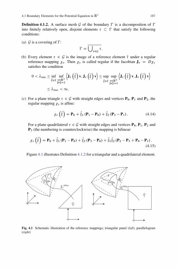
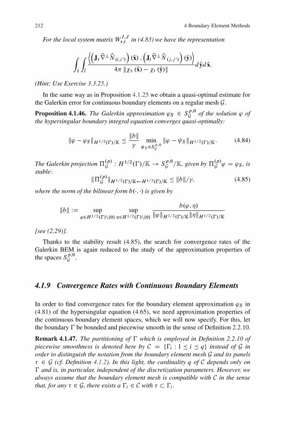
Figure 4.1 illustrates Definition 4.1.2 for a triangular and a quadrilateral element.
affine
affineaffine
Fig. 4.1 Schematic illustration of the reference mappings; triangular panel (left), parallelogram(right)
188 4 Boundary Element Methods
Exercise 4.1.3. Show the following:
(a) The affine mapping�� in (4.14) is regular if and only if P0, P1, P2 are vertices ofa non-degenerate (plane) triangle � , i.e., they are not colinear. Find an estimatefor the constants �min, �max from Definition 4.1.2(b) in terms of the interiorangles of � .
(c) Let P0;P1;P2;P3 be the vertices of a plane quadrilateral � with straight edges.The mapping �� from (4.15) is regular if all interior angles are smaller than �and larger than 0.
In some cases we will impose a compatibility condition for the intersection oftwo panels.
Definition 4.1.4. A surface mesh G of � is called regular if:
(a) The intersection of two different elements �; � 0 2 G is either empty, a commonvertex or a common side.
(b) The parametrizations of the panel edges of neighboring panels coincide: Forevery pair of different elements �; � 0 2 G with common edge e D � \ � 0 wehave
�� j Oe D �� 0 ı ��;� 0 j Oe ;where Oe WD ��1� .e/ and ��;� 0 W O� ! O� is a suitable affine bijection.
Remark 4.1.5. Throughout this section we assume that the boundary � is Lipschitzand admits a regular surface mesh in the sense of Definitions 4.1.2 and 4.1.4. Thisis a true restriction since not every Lipschitz surface admits a regular surface mesh.
For later error estimates we will introduce a few geometric parameters, whichrepresent a measure for the distortion of the panels as well as bounds for theirdiameters.
Assumption 4.1.6. There exist open subsets U; V � R3 and a diffeomorphism�� WU ! V with the following properties:
(a) � � U .(b) For every � 2 G, there exists a regular reference mapping �� W O� ! � of the
form�� D �� ı �affine
� W O� ! �;
where �affine� W R2 ! R3 is a regular, affine mapping.
Example 4.1.7.
1. Let � be a piecewise smooth surface that has a bi-Lipschitz continuous para-metrization over the polyhedral surface O�: �� W O� ! � . Let Gaffine WD˚� affinei W 1 � i � N � be a regular surface mesh of O� with the associated ref-
erence mappings �affine�affine W O� ! � affine. Then G WD ˚
���� affine
� W � affine 2 Gaffine�
defines a regular surface mesh of � which satisfies Assumption 4.1.6.
4.1 Boundary Elements for the Potential Equation in R3 189
2. For the unit sphere � WD ˚x 2 R3 W kxk D 1� one can choose the inscribed dou-ble pyramid with vertices .˙1; 0; 0/|, .0;˙1; 0/|, .0; 0;˙1/| as a polyhedralsurface O�, while �� W O� ! � is defined by �� .x/ WD x= kxk. By means of �� ,regular surface meshes on � can then be generated through lifting of regularsurface meshes of the polyhedral surface O� .
In order to construct a sequence of refined surface meshes for � , in many casesthe procedure is as follows.
Remark 4.1.8. Let � be the surface of a bounded Lipschitz domain � � R3. Inthe first step we construct a polyhedron O� along a bi-Lipschitz continuous map-ping �� W O� ! � (see Example 4.1.7). Let Gaffine
0 be a (very coarse) surfacemesh of O� . Then G0 WD
˚� D ��
�� affine
� W � affine 2 Gaffine0
�defines a coarse sur-
face mesh of � . We can obtain a sequence�Gaffine`
�`
of finer surface meshes if,during each refinement, we decompose every panel in Gaffine
0 into new panels bymeans of a fixed refinement method. For triangular elements, for example, weinterconnect the midpoints of the sides and for quadrilateral elements we connectboth pairs of opposite midpoints. This gives us a sequence of surface meshes byG` WD
˚� D ��
�� affine
� W � affine 2 Gaffine`
�.
Convention 4.1.9. If � and � affine appear in the same context the relation betweenthe two is given by � D ��
�� affine
�.
The following definition is illustrated in Fig. 4.2.
Definition 4.1.10. Let Assumption 4.1.6 be satisfied. The constants caffine > 0
(Caffine > 0) are the maximal (minimal) constants in
caffine kx� yk�k�� .x/� �� .y/k �Caffine kx � yk 8x; y 2 � affine;8� affine 2Gaffine
and describe the distortion of curved panels � compared to their affine pullbacks� affine.
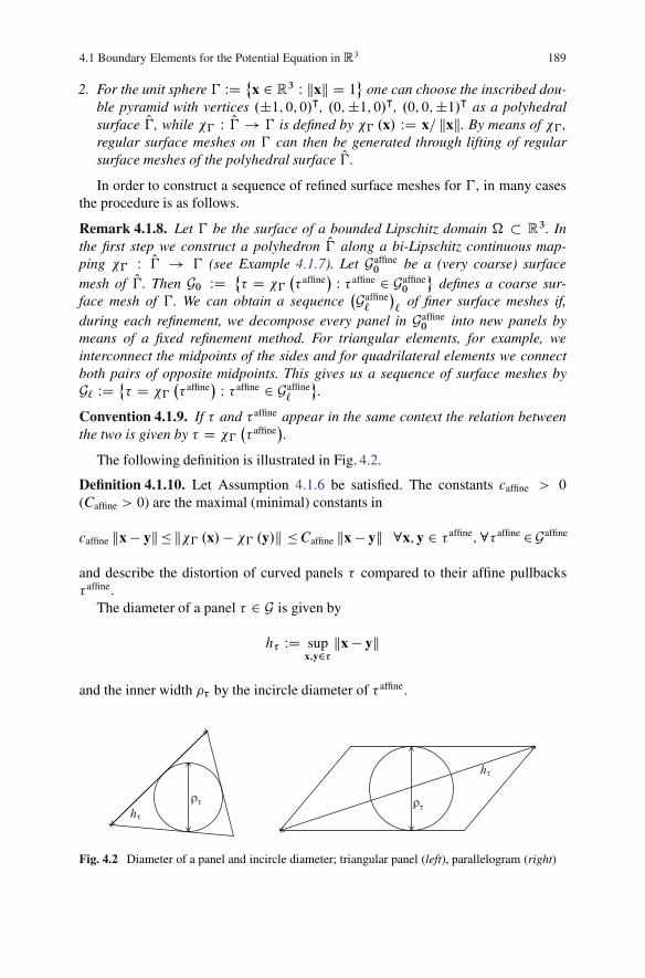
The diameter of a panel � 2 G is given by
h� WD supx;y2�kx � yk
and the inner width � by the incircle diameter of � affine.
Fig. 4.2 Diameter of a panel and incircle diameter; triangular panel (left), parallelogram (right)
190 4 Boundary Element Methods
The mesh width hG of a surface mesh G is given by
hG WD maxfh� W � 2 Gg: (4.16)
We write h instead of hG if the mesh G is clear from the context.
Remark 4.1.11. For plane panels � , � is the incircle diameter of � .The diameters of � and � affine satisfy
C�1affineh� � supx;y2�affine
kx � yk D h�affine � c�1affineh� :
Definition 4.1.12. The shape-regularity constant �G is given by
�G WD max�2G
h�
�: (4.17)
For some theorems we will assume, apart from the shape-regularity, that thediameters of all triangles are of the same order of magnitude.
Definition 4.1.13. The constant qG that describes the quasi-uniformity is given by
qG WD hG=min fh� W � 2 Gg :Remark 4.1.14. In order to study the convergence of boundary element methods,we will consider sequences .G`/`2N of surface meshes whose mesh width h` WD hG`
tends to zero. It is essential that the constant for the shape-regularity �` WD �G`
remains uniformly bounded above:
sup`2N
�` � � <1: (4.18)
In a similar way the constants of quasi-uniformity q` WD qG`have to be bounded
above in some theorems:sup`2N
q` � q <1: (4.19)
We call a mesh family .G`/`2N with the property (4.18) shape-regular and with theproperty (4.19) quasi-uniform.
Exercise 4.1.15. Show the following:
(a) If the surface mesh G0 is regular and if finer surface meshes .G`/` are con-structed according to the method described in Remark 4.1.8 then all surfacemeshes .G`/` are regular.
(b) The constants concerning shape-regularity and quasi-uniformity are, under theconditions in Part (a), uniformly bounded with respect to `.
4.1 Boundary Elements for the Potential Equation in R3 191
4.1.3 Discontinuous Boundary Elements
The boundary element method defines an approximation of the unknown density 'in the boundary integral equation (4.6) which is described by finitely many parame-ters. This can, for example, be achieved by (piecewise) polynomials on the elements� of a mesh G.
Example 4.1.16. (Piecewise Constant Boundary Elements)Let � D @� be piecewise smooth and let G be a – not necessarily regular –
surface mesh on � . Then S0G denotes all piecewise constant functions on the mesh G
S0G WD f 2 L1 .�/ j 8� 2 G W j� is constantg : (4.20)
Since 2 L1 .�/, we only need to define in the interior of an element, as theboundary @� , i.e., the set of edges and vertices of the panel, is a set of zero measure.
Every function 2 S0G is defined by its values � on the elements � 2 G and canbe written in the form
.x/ DX�2G
�b� .x/ (4.21)
with the characteristic function b� W � ! R of � 2 G:
b� .x/ WD(1 x 2 �;0 otherwise:
(4.22)
In particular, S0G is a vector space of dimension N D #f� W � 2 Gg with basisfb� W � 2 Gg.
In many cases the piecewise constant approximation of the unknown densityconverges too slowly and, instead, one uses polynomials of degree p � 1. In thesame way as in Example 4.1.16 this leads to the boundary element spaces SpG . Fortheir definition we need polynomials of total degree p on the reference element aswell as the convention for multi-indices from (2.67)
P�p D span˚� W 2 N2
0 ^ jj � p�: (4.23)
For p D 1 and p D 2, P�p contains all polynomials of the form
a00 C a101 C a012 8a00; a10; a01 2 R for p D 1;
a00 C a101 C a012 C a2021 C a1112 C a0222 8a00; a10; a01; a20; a11; a02 2 R for p D 2:
Definition 4.1.17. Let � D @� be piecewise smooth and let G be a surface meshof � . Then, for p 2 N0,
SpG WD
n W � ! K j 8� 2 G W ı �� 2 P�p
o: (4.24)
We simply write Sp or only S if the reference to the surface mesh G is obvious.
192 4 Boundary Element Methods
Remark 4.1.18. Note that in (4.24) the functions 2 Sp do not constitute poly-nomials on the surface � . Only once they have been “transported back” to thereference element O� by means of the element mapping �� (see Fig. 4.1) is this thecase. The parametrizations �� of the elements � 2 G in Definition 4.1.2 (b,c)are thus part of the set SpG . A change in parametrization �� will lead (with thesame mesh G) to a different SpG . Therefore for a mesh G we summarize the elementmappings �� in the mapping vector
� WD f�� W � 2 Gg (4.25)
and instead of (4.24) we write SpG;�.
Remark 4.1.19. Note that (4.24) also holds for meshes G with quadrilateral ele-ments, i.e., with reference element O� D .0; 1/2. Since Sp does not require continuityacross element boundaries, the space of polynomials P�p in (4.23) can also beapplied to quadrilateral meshes.
For the realization of the boundary element spaces we need a basis for P�p , which
we denote by bN .i;j /. O1; O2/ and which satisfies
P�p D spannbN .i;j / W 0 � i; j � p; i C j � p
o: (4.26)
For example, bN .i;j / .1; 2/ WD Oi1 Oj2 , 0 � i C j � p as in (4.23), would beadmissible basis functions.
Remark 4.1.20. (Nesting of Spaces)We have P�p � P�q for all p � q. Therefore we can always choose a basis in P�q
which contains the basis functions from P�p as a subset. The basis functions bN .i;j /
in (4.23) have this property.
Once we have determined a basis bN .i;j /. O/ on O� , every 2 SpG;� on a panel� 2 G can be written as
j� DX
0�iCj�p˛i;j
�bN .i;j / ı ��1��
andN �.i;j / WD bN .i;j / ı ��1� 0 � i C j � p
spans the restriction f j� W 2 Sp .�;G; �/g. In order to give a basis of SpG;�suitable indices, we define
�p WD˚ 2 N2
0 W jj � p�:
Thus we haveSpG;� D span
˚b.�;�/.x/ W .; �/ 2 �p � G� ; (4.27)
4.1 Boundary Elements for the Potential Equation in R3 193
where the global basis functions bI .x/ with the multi-index I D .; �/ denote thezero extension of the element functionN �
� to �: For
I D .; �/ 2 �p � G DW I .G; p/ DW I (4.28)
we explicitly have
bI .x/ WD(N ��.x/; x 2 �;
0 otherwise:(4.29)
Hence, every can be written as a combination of the basis function bI .x/:
.x/ DXI2I
I bI .x/; x 2 �; � 2 G: (4.30)
Let jGj be the number of elements in the mesh G. The dimension of SpG;� or thenumber of degrees of freedom is then given by
N D jGj .p C 1/.p C 2/=2 D dim.SpG;�/: (4.31)
Every function in 2SpG;� is then uniquely characterized by the vector . I /I2I.G;p/� RN Š RI.G;p/ as in (4.30).
4.1.4 Galerkin Boundary Element Method
The simplest boundary element method for Problem (4.6) consists in approximatingthe unknown density ' in (4.9) by a piecewise constant function 'S 2 S0.�;G/.Convention 4.1.21. The boundary element functions depend on the boundary ele-ment space Sp .�;G; �/; in particular, they depend on � , the surface mesh G andthe polynomial degree p. We will, whenever possible, use the abbreviated notation'S instead of 'Sp
G;�.
Inserting (4.30) into (4.6) or into the variational formulation (4.8) leads to a con-tradiction: since, in general, we have 'S 6D ', (4.6) and (4.8) cannot be satisfied with' D 'S , which is why the statements have to be weakened. As 'S is determinedby N parameters
�'SI�I2I [see (4.29)–(4.31)], we are looking for N conditions to
determine 'SI . In the Galerkin boundary element method we only let the test func-tion � run through a basis of SpG in the variational formulation of the boundaryintegral equation (4.9). The Galerkin approximation of the integral equation (4.9)then reads:
194 4 Boundary Element Methods
Find 'S 2 SpG;� such that
b.'S ; �S / D F.�S / 8�S 2 SpG;�; (4.32)
with b.�; �/ and F.�/ from (4.10) and (4.11) respectively.
Remark 4.1.22. (i) The Galerkin discretization (4.32) of (4.8) is achieved by res-tricting the trial and test functions '; � to the subspace SpG;� � H�1=2.�/ inthe variational formulation (4.8).
(ii) The boundary element solution 'S in (4.32) is independent of the basis chosenfor the subspace.
The computation of the approximation 'S requires that we choose a concretebasis for the subspace. Therefore, [see (4.29)–(4.31)] for a fixed p 2 N0, we choosethe basis
.bI W I 2 I .G; p// (4.33)
for SpG;�. Then (4.32) is equivalent to the linear system of equations:
Find ' 2 RN such thatB' D F: (4.34)
Here the system matrix B D .BI;J /I;J2I.G;p/ and the right-hand side F D.FJ /J2I.G;p/ 2 RN with I D .; �/ and J D .�; t/ are given by
BI;J WD b.bI ; bJ / (4.35)
DZ�
Z�
bJ .x/ bI .y/4� kx� yk dsy dsx D
Zt
Z�
N t� .x/N
��.y/
4� kx � yk dsy dsx
FJ WD F.bJ / DZ�
gD.x/bJ .x/ dsx DZt
gD.x/N t� .x/ dsx: (4.36)
Remark 4.1.23. The matrix B in (4.34) is dense because of (4.35), which meansthat all entriesBI;J are, in general, not equal to zero. Furthermore, the twofold sur-face integral in (4.35) can very often not be computed exactly, even for polyhedrons,and requires numerical integration methods for its approximation. The influence ofthis additional approximation will be discussed in Chap. 5. In this chapter we willalways assume that the matrix B can be determined exactly.
Proposition 4.1.24. The system matrix B in (4.34) is symmetric and positive defi-nite.
Proof. From the symmetry of b.'; �/ D b.�; '/ we immediately have
BI;J D b.bI ; bJ / D b.bJ ; bI / D BJ;I ;
and subsequently B D B|. Now let ' 2 RN be arbitrary. Then we have
4.1 Boundary Elements for the Potential Equation in R3 195
'|B' DX
I;J2I.G;p/'J'IBI;J D
XI;J
'J'Ib.bI ; bJ / D b X
I
'IbI ;XJ
'J bJ
!
D b.'S ; 'S / � �k'Sk2H�1=2.�/> 0
if and only if 'S 6D 0. Since fbI W I 2 Ig is a basis of Sp, we have 'S 6D 0 if andonly if ' 6D 0 2 RN . Therefore B is positive definite. �
Thus the discrete problem (4.32) or (4.34) has a unique solution 'S 2 SpG .The following proposition supplies us with an estimate for the error ' � 'S .
Proposition 4.1.25. Let ' be the exact solution of (4.9). The Galerkin solution 'Sof (4.32) converges quasi-optimally
k' � 'SkH�1=2.�/ �kbk�
minS2Sp
k' � �SkH�1=2.�/: (4.37)
The error satisfies the Galerkin orthogonality
b.' � 'S ; �S / D 0 8�S 2 Sp : (4.38)
Proof. We will first prove the statement in (4.38). If we only consider (4.10) for testfunctions from Sp we can subtract (4.32) and obtain
b.' � 'S ; �S / D b.'; �S /� b.'S ; �S / D F.�S /� F.�S / D 0 8�S 2 Sp:
Next we prove (4.37). For the error eS D ' � 'S we have by the ellipticity andthe continuity of the boundary integral operator V and (4.38)
�k' � 'Sk2H�1=2.�/� b.eS ; eS / D b.eS ; ' � 'S/D b.eS ; '/ � b.eS ; 'S / D b.eS ; '/ � b.eS ; �S / D b.eS ; ' � �S/� kbkkeSkH�1=2.�/k' � �SkH�1=2.�/
for all �S 2 Sp .If we cancel keSkH�1=2.�/ and minimize over �S 2 Sp we obtain the assertion
(4.37). �The inequality in (4.37) shows that the Galerkin error k' � 'SkH�1=2.�/ coin-
cides with the error of the best approximation of ' in Sp up to a multiplicativeconstant. This is where the term quasi-optimality for the a priori error estimate(4.37) originates.
Remark 4.1.26 (Collocation). We obtained the Galerkin discretization (4.32) from(4.8) by restricting the trial and test functions '; � to the subspace Sp � S .Alternatively, one can insert 'S into (4.6) and impose the equation
196 4 Boundary Element Methods
.V'S/.xJ / D gD.xJ / J 2 I .G; p/ (4.39)
only in N collocation points fxJ W J 2 Ig. The solvability of (4.39) dependsstrongly on the choice of collocation points fxJ W J 2 Ig. Equation (4.39) is alsoequivalent to a linear system of equations, where the entries of the system matrixBcol l are defined by
Bcol lI;J WDZ�
bJ .y/4� kxI � ykdsy: (4.40)
Note that Bcol l is again dense, but not symmetric.The collocation method (4.39) is widespread in the field of engineering, because
the computation of the matrix entries (4.40) only requires the evaluation of oneintegral over the surface � , instead of, as with the Galerkin method, a twofold inte-gration over � . However, the stability and convergence of collocation methods onpolyhedral surfaces is still an open question, especially with integral equations ofthe first kind. For integral operators of zero order or equations of the second kindwe only have stability results in some special cases. For a detailed discussion oncollocation methods we refer to, e.g., [6, 8, 87, 187, 207, 215] and the referencescontained therein.
We now return to the Galerkin method.
Remark 4.1.27 (Stability of the Galerkin Projection). The Galerkin method(4.32) defines a mapping
…pS W H�1=2.�/! S
pG;� W …
pS' WD 'S ;
which is called the Galerkin projection. Clearly, …pS is linear and because of the
ellipticity of the boundary integral operator V we have
�k…pS'k2H�1=2.�/
D �k'Sk2H�1=2.�/� b.'S ; 'S / D b.'; 'S/
� kbkk'kH�1=2.�/k…pS'kH�1=2.�/;
from which we have, after canceling, the boundedness of the Galerkin projection…pS W H�
12 .�/! H� 1
2 .�/ independent of the mesh G:
k…pS'kH�1=2.�/ �
kbk�k'kH�1=2.�/: (4.41)
The quasi-optimality (4.37) and the boundedness of the Galerkin projectioncombined with the following corollary give us the convergence of the GalerkinBEM.
Corollary 4.1.28. Let .G`/`2N be a sequence of meshes on � with a mesh widthh` D hG`
and let h` ! 0 for ` ! 1. Then the sequence .'`/`2N of boundaryelement solutions (4.32) in S` D SpG`
converges to ' for every fixed p 2 N0.
4.1 Boundary Elements for the Potential Equation in R3 197
Proof. Since S0`� Sp
`for all p 2 N0, we will only consider the case p D 0. S0
`are
step functions on meshes whose mesh width converges to zero. The density followsfrom the construction of the Lebesgue spaces
[`2N
S0`
k�kL2.�/ D L2 .�/
and from Proposition 2.5.2 we have the dense embeddingL2 .�/ � H�1=2.�/.For ' 2 H�1=2 .�/ and an arbitrary " > 0 we can therefore choose a Q' from
L2 .�/ and an ` 2 N , combined so that Q'` 2 S0` , such that
k' � Q'kH�1=2.�/ � "=2 and k Q' � Q'`kL2.�/ � "=2:
From this we have
k' � Q'`kH�1=2.�/ � k' � Q'kH�1=2.�/ C k Q' � Q'`kH�1=2.�/ �"
2C "
2� ":
The quasi-optimality of the Galerkin method gives us
k' � '`kH�1=2.�/ �kbk�k' � Q'`kH�1=2.�/ � "
kbk�:
As " > 0 is arbitrary, we have the assertion for `!1. �
4.1.5 Convergence Rate of Discontinuous Boundary Elements
We have seen in Proposition 4.1.25 that the approximations 'S 2 S from theGalerkin boundary element method approximate the exact solution ' of the equa-tion of the first kind (4.9) quasi-optimally: the error ' � 'S , which is measured inthe “natural”H�1=2.�/-norm, is – up to a multiplicative constant – just as large as
min˚k' � SkH�1=2.�/ W S 2 S
�(4.42)
which is the error of the best approximation in the space S . The convergence rate ofthe BEM indicates how fast the error converges to zero in relation to an increase inthe degrees of freedomN . Here we will only prove the convergence rate for p D 0,while the general case will be treated in Sect. 4.3. We begin with the second Poincareinequality on the reference element O� .
Convention 4.1.29. Variables on the reference element are always marked by a“ˆ”. If the variables x 2 � and Ox 2 O� appear in the same context this shouldalways be understood in terms of the relation x D �� .Ox/. Derivatives with respectto variables in the reference element are also marked by a “ˆ”. We will write, forexample, br as an abbreviation for rOx . Should the functions u W � ! K and Ou W O� !K appear in the same context, they are connected by the relation u ı �� D Ou.
198 4 Boundary Element Methods
Proposition 4.1.30. Let O� � R2 be the reference element, O' 2 H 1. O�/ and O'0 WD1j O� jRO� O' d Ox. Then there exists some Oc > 0 such that
k O' � O'0kL2. O�/ � Ockbr O'kL2. O�/; (4.43)
where Oc depends only on O� .
Proof. The assertion follows directly from the proof of Corollary 2.5.10. �In the following we will derive error estimates for a simplified situation. We will
discuss the general case in Sect. 4.3. Here we let � be a plane manifold in R3 witha polygonal boundary. As integrals are invariant under rotation and translation, weassume without loss of generality that
� is a two-dimensional polygonal domain, (4.44)
i.e., we restrict ourselves to the two-dimensional approximation problem in theplane.
Furthermore, let G D f�i W 1 � i � N g be a surface mesh on � of shape-regulartriangles with straight edges and with mesh width h > 0. Then the triangles � 2 Gare affinely equivalent to the reference element O� via the transformation (4.14):
� 3 x D �� .Ox/ D P0 C JOx; Ox 2 O�; (4.45)
where J is the matrix with the columns P1 � P0 and P2 � P1 (see Fig. 4.1). With(4.45) and the chain rule
@
@x˛D @
@ Ox1@ Ox1@x˛C @
@ Ox2@ Ox2@x˛
˛ D 1; 2;
the relationr D �J�1�| br; dx D .det J/ d Ox D 2 j� j d Ox (4.46)
follows. This leads to the transformation formula for Sobolev norms
kbr O'k2L2. O�/ D
ZO�jbr O'j2 d Ox D jO� jj� j
Z�
.r'/>JJ>.r'/dx
� jO� jj� j��Z�
kr'k2 dx; (4.47)
where �� denotes the largest eigenvalue of JJ| 2 R2�2. Furthermore, we have forthe left-hand side of (4.43)
k O' � O'0k2L2. O�/ DjO� jj� j k' � '0k
2L2.�/
(4.48)
4.1 Boundary Elements for the Potential Equation in R3 199
with '0 WD 1j� jR�'dx. If we combine (4.48) with (4.43) and (4.47) we obtain
k' � '0k2L2.�/ Dj� jj O� j k O' � O'0k
2L2.O�/� Oc2 j� jj O� j k
br O'k2L2.O�/� Oc2�� kr'k2L2.�/ 8� 2 G:
(4.49)Exercise 4.1.32 shows that
�� � kP1 � P0k2 C kP2 � P1k2 � 2h2� : (4.50)
From this we havek' � '0kL2.�/ �
p2 Och� j'jH1.�/: (4.51)
Squaring and then summing over all � 2 G leads to the following error estimate.
Proposition 4.1.31. Let (4.44) hold. Let G be a surface mesh of � . Let ' 2 L2.�/with 'j� 2 H 1.�/ for all � 2 G. Then we have the error estimate
min 2S0
Gk' � kL2.�/ �
p2 Oc X�2G
h2� j'j2H1.�/
!1=2: (4.52)
For ' 2 H 1.�/ the error estimate can be simplified to
min 2S0
Gk' � kL2.�/ �
p2 OchG j'jH1.�/: (4.53)
Exercise 4.1.32. Let � be a plane triangle with straight edges in R2 with verticesP0, P1, P2. Let the matrix J and the eigenvalue �� be defined as in (4.45) and (4.47)respectively. Show that
�� � kP1 � P0k2 C kP2 � P1k2 :
From the approximation property we will now derive an error estimate for theGalerkin solution.
Theorem 4.1.33. Let � be the surface of a polyhedron. Let the surface mesh Gconsist of triangles with straight edges.
For the solution ' of the integral equation of the first kind (4.6) we assume thatfor an 0 � s � 1 we have
' 2 H s.�/: (4.54)
Then the Galerkin approximation 'S 2 S0G satisfies the error estimate
k' � 'SkH�1=2.�/ � C hsC1=2k'kH s.�/: (4.55)
Proof. The conditions of the theorem allow us to apply Proposition 4.1.31. With(4.37) we obtain for the Galerkin solution 'S the error estimate

200 4 Boundary Element Methods
k' � 'SkH�1=2.�/ D k' �…0S 'kH�1=2.�/ �
kbk�
min S2S0
Gk' � SkH�1=2.�/:
The definition of the H�1=2 .�/-norm gives us
k' � SkH�1=2.�/ D sup2H1=2.�/nf0g
.' � S ; �/L2.�/
k�kH1=2.�/
: (4.56)
We will first consider the case ' 2 H 1.�/ and choose S elementwise as the meanvalue of '
P' WD S with S j� WD1
j� jZ�
' dx; � 2 G;
i.e., P is the L2-orthogonal projection onto S0G . Hence it follows from Proposi-tion 4.1.31 that
k SkL2.�/�k'kL2.�/; k' � SkL2.�/� 2k'kL2.�/; k' � SkL2.�/� chk'kH1.�/:
(4.57)
If in Proposition 2.1.62 we choose T D I � P we have T W L2 .�/ ! L2 .�/
and T W H 1 .�/! L2 .�/. For the norms we have, by (4.57), the estimates
kT kL2.�/ L2.�/ � 2 and kT kL2.�/ H1.�/ � ch:
Proposition 2.1.62 implies that T W H s .�/! L2 .�/ for all 0 � s � 1 and that
kT kL2.�/ H s.�/ � chs :
This is equivalent to the error estimate
k' � SkL2.�/ � c hsk'kH s.�/: (4.58)
In order to derive an error estimate for the H�1=2 .�/-norm, we use (4.56) and notethat the equality
j .' � S ; �/L2.�/ j D j .' � S ; � � �S /L2.�/ j
holds for an arbitrary �S 2 S0G . By using ' 2 H s.�/, � 2 H 1=2.�/ and (4.58) andby choosing �S elementwise as the integral mean value of �, we obtain the estimate
ˇ.' � S ; �/L2.�/
ˇ D ˇ.' � S ; � � �S /L2.�/
ˇ � k' � SkL2.�/ k� � �SkL2.�/
� chsk'kH s.�/h1=2k�kH1=2.�/:
�
4.1 Boundary Elements for the Potential Equation in R3 201
The error estimate (4.55) shows that the convergence rate hsC1=2 of the BEMdepends on the regularity of the solution '. In Sect. 3.2 we stated the regularity –the maximal s > 0 such that ' 2 H�1=2Cs .�/ – without knowing the exact solu-tion ' explicitly. Ideally, ' is smooth on the entire surface .s D 1) or at leaston every panel. The convergence rate would then be bounded by the polynomialorder p of the boundary elements, due to the fact that the following generalizationof Theorem 4.1.33 holds.
Corollary 4.1.34. Let the exact solution of (4.9) satisfy ' 2 H s.�/ for an s � 0.Then the boundary element solution 'S 2 SpG satisfies the error estimate
k' � 'SkH�1=2.�/ � ch1=2Cmin.s;pC1/G k'kH s.�/; (4.59)
for a surface mesh G of the boundary � , which consists of triangles with straightedges. Here the constant c depends on p and the shape-regularity of the surfacemesh.
The proof of Corollary 4.1.34 will be completed in Sect. 4.3.4 (see Remark4.3.21).
4.1.6 Model Problem 2: Neumann Problem
Let �� � R3 be a bounded interior domain with boundary � and �C WD R3n��.For gN 2 H�1=2.�/ we consider the Neumann problem
�u D 0 in �C; (4.60)
�1u D gN on �; (4.61)
ju .x/j � C kxk�1 for kxk ! 1: (4.62)
The exterior problem (4.60)–(4.62) has a unique solution u, which can berepresented as a double layer potential
u.x/ D 1
4�
Z�
'.y/@
@ny
1
kx � yk dsy; x 2 �C: (4.63)
Thanks to the jump relations (see Corollary 3.3.12)
1
4�
Z�
@
@ny
1
kx � yk dsy D
8<ˆ:
�1 x 2 ��;�12
x 2 � and � is smooth in x
0 x 2 �C
202 4 Boundary Element Methods
u.x/ in (4.63) does not change if a constant is added to '. If we put (4.63) into theboundary condition (4.61) we obtain the equation
�W' D @
@nx
�1
4�
Z�
'.y/@
@ny
1
kx � yk dsy
�D gN .x/; x 2 �: (4.64)
The following remark shows that the derivative @=@nx and the integral do notcommute.
Remark 4.1.35. The normal derivative @=@nx, applied to the kernel in (4.64), yields
@2
@nx@ny
1
kx � yk D˝nx;ny
˛kx � yk3 � 3
hnx; x � yi ˝ny; x � y˛
kx � yk5 :
Therefore the kernel of the associated hypersingular integral operator is not inte-grable.
There are three possibilities of representing the integral operator W' on thesurface: (a) by extending the definition of an integral to strongly singular kernelfunctions (see [201, 211]), (b) by integration by parts (see Sect. 3.3.4) and (c) byintroducing suitable differences of test and trial functions (see [117, Sect. 8.3]). Inthis section we will consider option (b). The notation and theorems from Sect. 3.3.4can be simplified for the Laplace problem, so that they read
curl� ' WD �0 .gradZ�'/ � n;
b.'; �/ DZ�
Z�
hcurl� ' .y/; curl� � .x/i4� kx � yk dsydsx;
where Z� W H 1=2 .�/ ! H 1 .��/ is an arbitrary extension operator (see Theo-rem 2.6.11 and Exercise 3.3.25).
The variational formulation of the boundary integral equation is given by (seeTheorem 3.3.22): Find ' 2 H 1=2.�/=K such that
b.'; �/ D � .gN ; �/L2.�/ 8� 2 H 1=2.�/=K: (4.65)
In Theorem 3.5.3 we have already shown that the density ' in (4.63) is the uniquesolution of the boundary integral equation (4.65). The proof was based on the factthat the bilinear form b .�; �/ is symmetric, continuous andH 1=2 .�/ =K-elliptic.
4.1.7 Continuous Boundary Elements
The Galerkin method is based on the concept of replacing the infinite-dimensionalHilbert space by a finite-dimensional subspace. The bilinear form that is asso-ciated with the hypersingular integral operator is defined on the Sobolev space
4.1 Boundary Elements for the Potential Equation in R3 203
H 1=2 .�/ =K. As the discontinuous boundary element functions from Example4.1.16 and Definition 4.1.17 are not contained in H 1=2 .�/ =K (see Exercise 2.4.4),we will introduce continuous boundary element spaces for the Neumann problem.
We again start with a mesh G on the boundary � . In order to define continuousboundary elements, we assume (see Definition 4.1.4):
The surface mesh G is regular. (4.66)
This means that the intersection � \ � 0 of two different panels is either empty, avertex or an entire edge. Furthermore, the boundary elements are either trianglesor quadrilaterals and are images of the reference triangle or quadrilateral O� respec-tively (see Fig. 4.1). Note that the boundary edges of the panels “have the sameparametrization on both sides” in the case of continuous boundary elements (seeDefinition 4.1.4).
We assume that the boundary � is piecewise smooth (see Definition 2.2.10 andFig. 4.1) so that the reference mappings �� W O� ! � can be chosen as smooth dif-feomorphisms. As in the case for discontinuous boundary elements, the continuousboundary elements are also piecewise polynomials on the surface � . When usingdiscontinuous elements, a boundary element function 'S is locally a polynomial ofdegree p in each element � 2 G:
8� 2 GW 'S ı �� 2 P�p . O�/:
With continuous elements we have for � 2 G:
'S ı �� 2 P �p WD8<:
P�p if � is a triangular element,
P �p if � is a quadrilateral element,
(4.67)
where for p � 1 the polynomial space P�p is defined as in (4.23) and
P �p WD spanf Oi1 Oj2 W 0 � i; j � pg:
Now we come to the definition of continuous boundary element functions ofdegree p � 1.
Definition 4.1.36. Let � be a piecewise smooth surface, G a regular surface meshof � and � D f�� W � 2 Gg the mapping vector. Then the space of continuousboundary elements of degree p � 1 is given by
Sp;0G;� WD f' 2 C 0.�/ j 8� 2 G W 'j� ı �� 2 P �pg:
In order to make the distinction between continuous and discontinuous boundaryelements of degreep we will from now on denote discontinuous elements by Sp;�1G;� .
204 4 Boundary Element Methods
Just like the space Sp;�1 of discontinuous boundary elements, the space Sp;0 isalso finite-dimensional. In the following we will introduce a basis f'I W I 2 Ig ofSp;0. In contrast to Sp;�1, the support of the basis functions in general consists ofmore than one panel and the basis functions are defined piecewise on those panels.We begin with the simplest case, p D 1.
Example 4.1.37. (Linear and Bilinear, Continuous Boundary Elements)The shape functions bN.Ox/, Ox D . Ox1; Ox2/ on the reference element O� are:
� In the case of the unit triangle with vertices P0 D .0; 0/|, P1 D .1; 0/|, P2 D.1; 1/| [see (4.13)], given by
bN 0.Ox/ D 1 � Ox1; (4.68)
bN 1.Ox/ D Ox1 � Ox2;bN 2.Ox/ D Ox2
and� In the case of the unit square with vertices P0 D .0; 0/|, P1 D .1; 0/|, P2 D.1; 1/|, P3 D .0; 1/|, given by
bN 0.Ox/ D .1 � Ox1/.1 � Ox2/; (4.69)
bN 1.Ox/ D Ox1.1 � Ox2/;bN 2.Ox/ D .1 � Ox1/ Ox2;bN 3.Ox/ D Ox1 Ox2:
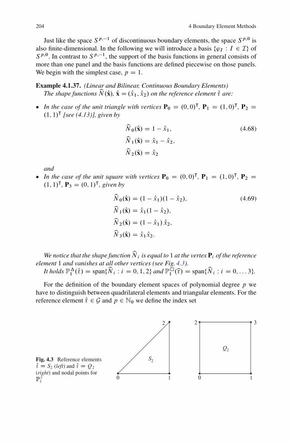
We notice that the shape function bN i is equal to 1 at the vertex Pi of the referenceelement 1 and vanishes at all other vertices (see Fig. 4.3).
It holds P�1 . O�/ D spanfbN i W i D 0; 1; 2g and P �1 .b�/ D spanfbN i W i D 0; : : : 3g.
For the definition of the boundary element spaces of polynomial degree p wehave to distinguish between quadrilateral elements and triangular elements. For thereference element O� 2 G and p 2 N0 we define the index set
Fig. 4.3 Reference elementsO� D S2 (left) and O� D Q2
(right) and nodal points forP O�1
1 1
2
2
4.1 Boundary Elements for the Potential Equation in R3 205
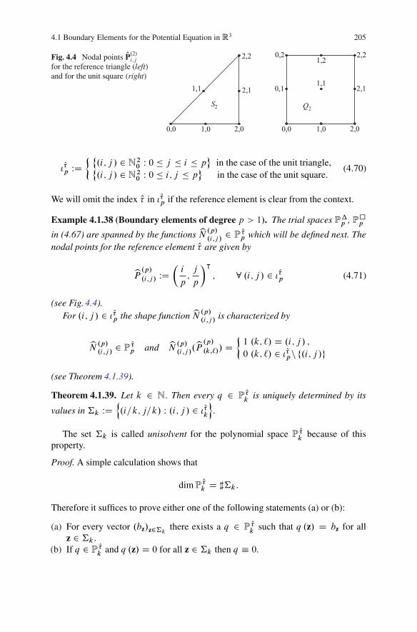
Fig. 4.4 Nodal points OP.2/i;jfor the reference triangle (left)and for the unit square (right)
2,1
1,0 1,0
1,1 0,1 2,1
1,2
1,1
� O�p WD ˚.i; j / 2 N2
0 W 0 � j � i � p�
in the case of the unit triangle,˚.i; j / 2 N2
0 W 0 � i; j � p�
in the case of the unit square.(4.70)
We will omit the index O� in � O�p if the reference element is clear from the context.
Example 4.1.38 (Boundary elements of degree p > 1). The trial spaces P�p , P �p
in (4.67) are spanned by the functions bN .p/
.i;j /2 P O�p which will be defined next. The
nodal points for the reference element O� are given by
bP .p/.i;j / WD�i
p;j
p
�|; 8 .i; j / 2 � O�p (4.71)
(see Fig. 4.4).For .i; j / 2 � O�p the shape function bN .p/
.i;j /is characterized by
bN .p/
.i;j /2 P O�p and bN .p/
.i;j /.bP .p/.k;`// D
1 .k; `/ D .i; j / ;0 .k; `/ 2 � O�pn f.i; j /g
(see Theorem 4.1.39).
Theorem 4.1.39. Let k 2 N . Then every q 2 P O�k
is uniquely determined by its
values in †k WDn.i=k; j=k/ W .i; j / 2 � O�
k
o.
The set †k is called unisolvent for the polynomial space P O�k
because of thisproperty.
Proof. A simple calculation shows that
dim P O�k D ]†k:
Therefore it suffices to prove either one of the following statements (a) or (b):
(a) For every vector .bz/z2†kthere exists a q 2 P O�
ksuch that q .z/ D bz for all
z 2 †k:(b) If q 2 P O�
kand q .z/ D 0 for all z 2 †k then q 0.
206 4 Boundary Element Methods
Case 1: O� D .0; 1/2: For 2 � O�k
we define the function bN� by
bN� .x/ WD Q2jD1
QkijD0ij¤�j
kxj � ijj � ij :
Then bN� 2 P O�k
with bN� .=k/ D 1 and bN�
�i1k; i2k
�D 0 for all .i1; i2/ 2 � O�kn fg.
Now let�b���2 O�
k
be arbitrary. Then the polynomial q 2 P O�k
q .x/ DX�2 O�p
b�bN� .x/
satisfies property (a).Case 2: O� is the reference triangle. As in Example 4.1.37 we set
O�1 .x/ WD 1 � Ox1; O�2 .x/ WD Ox1 � Ox2; O�3 .x/ WD Ox2:
Clearly, these functions are in P O�1 and have the Lagrange property
81 � i; j � 3 W O�i�Aj� D ıi;j with A1 D .0; 0/| , A2 D .1; 0/| , A3 D .1; 1/| :
1. k D 1W For a given .bi /3iD1 2 R3, q 2 P1W
q .x/ D3XiD1
bi O�i .x/
clearly has the property (a).2. k D 2W For 1 � i < j � 3, A.i;j / WD
�Ai C Aj
�=2 denote the midpoints of the
edges of O� . We define
bN i WD O�i�2 O�i � 1
�1 � i � 3;
bN .i;j / WD 4 O�i�j 1 � i < j � 3:
Then we clearly have bN k , bN .i;j / 2 P O�2 and
bN i
�Aj� D ıi;j bN i
�A.k;`/
� D 0 8i; k; `;bN .i;j / .Ak/ D 0 bN .i;j /
�A.k;`/
� D ıi;kıj;` 8i; j; k; `:For a given fbz W z 2 †2g D
˚bi ; b.k;`/
�, the polynomial q 2 P O�2 defined by
q .x/ WD3XiD1
bibN i .x/CX
1�k<`�3b.k;`/bN .k;`/ .x/
has the property (a).
4.1 Boundary Elements for the Potential Equation in R3 207
3. k D 3W This case will be treated in Exercise 4.1.40.4. k � 4W Let q 2 P�
kwith q .z/ D 0 for all z 2 †k . Then q vanishes on all edges
of O� . Therefore there exists a 2 P�k�3 such that
q D O�1 O�2 O�3 and 8z 2 †k \ O� W .z/ D 0:
(Note that O� is open.) The problem can thus be reduced to
� 2 P�k�3
�^ .8z 2 †k \ O� W .z/ D 0/ H) 0: (4.72)
Property (b) follows by induction over k as follows.
Let O� 0 be the triangle with vertices A D �2kC1 ;
1kC1
�|, B D
�kkC1 ;
1kC1
�|, C D�
kkC1 ;
k�1kC1
�|. Then we have †k \ O� DW †0k �b� 0. The transformation
T W O� ! O� 0 W T D AC�1� 3
k C 1�
is affine and therefore Q D ı T 2 P�k�3. Furthermore, we have T �1†0
kD
†k�3. Hence (4.72) is equivalent to
� Q 2 P�k�3�^ �8z 2 †k�3 W Q .z/ D 0
� H) Q 0:
This, however, is statement (b) for k k � 3. Since the induction hypothesisfor k D 1; 2; 3 is given by steps 1–3 in the proof, the assertion follows by virtueof the equivalence of the two statements (a) and (b). �
Exercise 4.1.40. Let O� be the unit triangle. For P O�3 construct a Lagrange basis forthe set of mesh points †3 (see Theorem 4.1.39).
In combination with the polynomial space P O�p on O� we define an interpolation
operator bIp for the set of nodal points †p D�bP .p/.i;j /
�.i;j /2p
for continuous
functions ' 2 C 0�O��
by
bIp' WD X.i;j /2 O�p
'�bP .p/.i;j /
� bN .p/
.i;j /: (4.73)
The Sobolev embedding theorem (Theorem 2.5.4) proves the continuity of the
embedding H t . O�/ ,! C 0�O��
thanks to O� � R2 for t > 1 and therefore bIp is
defined on H t . O�/, thus
208 4 Boundary Element Methods
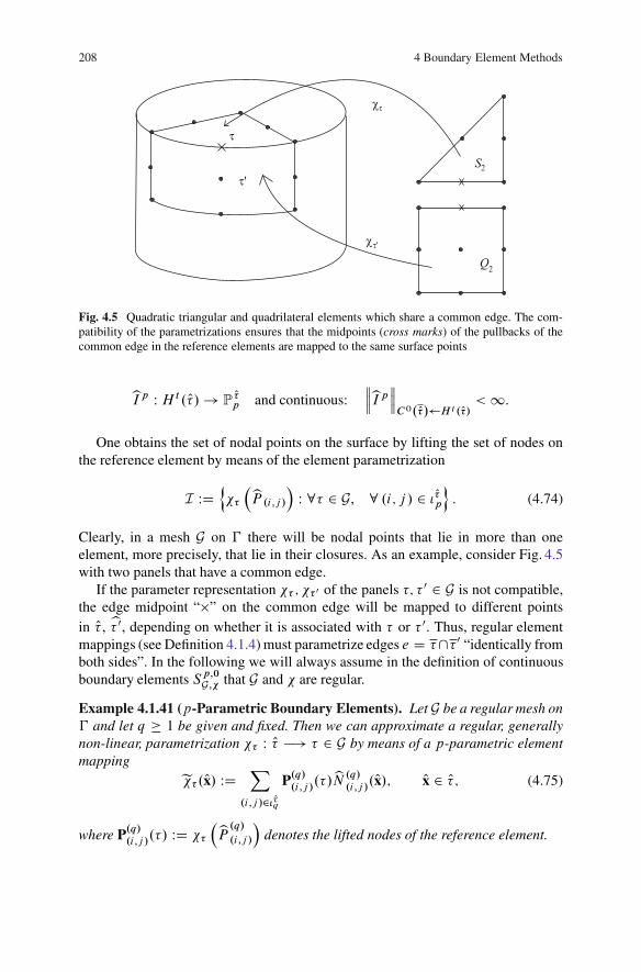
Fig. 4.5 Quadratic triangular and quadrilateral elements which share a common edge. The com-patibility of the parametrizations ensures that the midpoints (cross marks) of the pullbacks of thecommon edge in the reference elements are mapped to the same surface points
bIp W H t . O�/! P O�p and continuous:bIp
C0. O�/ H t .O�/ <1:
One obtains the set of nodal points on the surface by lifting the set of nodes onthe reference element by means of the element parametrization
I WDn��
�bP .i;j /�W 8� 2 G, 8 .i; j / 2 � O�p
o: (4.74)
Clearly, in a mesh G on � there will be nodal points that lie in more than oneelement, more precisely, that lie in their closures. As an example, consider Fig. 4.5with two panels that have a common edge.
If the parameter representation �� ; �� 0 of the panels �; � 0 2 G is not compatible,the edge midpoint “�” on the common edge will be mapped to different pointsin O� , b� 0, depending on whether it is associated with � or � 0. Thus, regular elementmappings (see Definition 4.1.4) must parametrize edges e D �\� 0 “identically fromboth sides”. In the following we will always assume in the definition of continuousboundary elements Sp;0G;� that G and � are regular.
Example 4.1.41 (p-Parametric Boundary Elements). Let G be a regular mesh on� and let q � 1 be given and fixed. Then we can approximate a regular, generallynon-linear, parametrization �� W O� �! � 2 G by means of a p-parametric elementmapping
e�� .Ox/ WD X.i;j /2 O�q
P.q/.i;j /
.�/bN .q/
.i;j /.Ox/; Ox 2 O�; (4.75)
where P.q/.i;j /
.�/ WD ���bP .q/.i;j /
�denotes the lifted nodes of the reference element.
4.1 Boundary Elements for the Potential Equation in R3 209
Remark 4.1.42. In practical applications the construction (4.75) is used for p D 1and p D 2 with the shape functions bN .p/
.i;j /for the set of points bP .p/.i;j / in (4.71). In
every case the approximation panel Q� WDe�� . O�/ interpolates the exact panel � at thepoints P.p/
.i;j /. It is known from interpolation theory (see Sect. 7.1.3.1) that, for the
quality of the approximation, the choice of interpolation points becomes essentialfor high orders of approximation such as p � 3. For p � 3 the images of theGauss–Lobatto points for the unit square represent a better choice for the set ofnodes P.p/
.i;j /. Similar sets of points are known for the unit triangle (see [16, 130]).
In the following we will always assume that the � describe the surface � exactly.The influence of the approximation of the domain on the accuracy of the boundaryelement solution is discussed in Chap. 8.
We define the space of the continuous, piecewise polynomial boundary elementsof degree p � 1 by a basis bI . For this, let I be, as in (4.74), the set of all nodalpoints in the mesh G. The basis function bP for the nodal point P 2 I is characterizedby the conditions
bP 2 Sp;0G and bP.P0/ WD(1 for P0 D P;
0 for P0 6D P; P0 2 I:(4.76)
For a nodal point P 2 I we define a local neighborhood of triangles by �P WDSf� W � 2 G; P 2 �g. Then we have
supp.bP/ D �P: (4.77)
In order to derive a local representation of the basis functions by element shapefunctions, we need a relation between global indices P 2 I and local indices .i; j / 2� O�p. For � 2 G and I D .i; j / 2 � O�p we define a mapping ind W G � � O�p ! I by
ind .�; I / WD ���bP .i;j /
�2 I. (4.78)
With this we have, for � 2 G, I D .i; j / 2 � O�p and P D ind .�; I / 2 I, the relation
bPj� D N �.i;j / WD bN I ı ��1� : (4.79)
In the following we will show that the functions in Sp;0G;� are Lipschitz continuousand are thus contained in H 1 .�/. In order to compare the Euclidian distance withthe surface distance, we introduce the geodesic distance
dist� .x; y/ WD inf˚length
��x;y
� W �x;y is a path in � that connects x and y�
and the constant g�
210 4 Boundary Element Methods
g� WD supx;y2�
dist� .x; y/kx � yk
�: (4.80)
Remark 4.1.43. The functions 'S 2 Sp;0G;� are Lipschitz continuous
j'S .x/� 'S .y/j � C kx � yk 8x; y 2 �;
where C depends on � , G, � and g� .
Proof. The continuity of 'S 2 Sp;0G;� follows directly from the definition so that weonly need to prove the Lipschitz continuity. Let x; y 2 � and let �x;y be a connectingpath with minimal length on � . Let
��j�qjD0 � G be a minimal subset of G with the
property:
x 2 �0, y 2 �q , �x;y �q[jD1
�j
81 � j � q W �j�1 \ �j is a common edge ej and ej \ �x;y ¤ ;.
We fix the points Mj on ej \ �x;y, 1 � j � q and set M0 D x and MqC1 D y.
Without loss of generality we assume that all�Mj
�qC1jD0 are distinct; otherwise we
simply eliminate points that appear in the sequence more than once. Then, by thecontinuity of 'S , we have
'S .y/� 'S .x/ D 'S�MqC1
� � 'S .M0/ DqXjD0
�'S�MjC1
� � 'S �Mj
��:
The points MjC1, Mj are in the panel �j . Since 'S j� is the composition of apolynomial with a diffeomorphism, these restrictions are Lipschitz continuous. With
c� WD supx;y2�
j'S .x/� 'S .y/jkx � yk
we have
ˇ'S�MjC1
� � 'S �Mj
�ˇ � c� MjC1 �Mj
� c�L ��Mj ;Mj C1
�;
where L��Mj ;Mj C1
�denotes the length of the shortest connecting path in � that
connects Mj with MjC1. Finally, with (4.80) we have
j'S .y/� 'S .x/j ��
max1�j�q c�j
�L��x;y
� � g��
max1�j�q c�j
�kx � yk ;
which is the Lipschitz continuity of 'S . �
4.1 Boundary Elements for the Potential Equation in R3 211
4.1.8 Galerkin BEM with Continuous Boundary Elements
The inclusion Sp;0G;� � H 1=2 .�/ of the continuous boundary elements permits theGalerkin discretization of the hypersingular boundary integral equation:Find 'S 2 Sp;0G =K such that
b.'S ; �S / D .gN ; �S /L2.�/ 8�S 2 Sp;0G =K: (4.81)
The ellipticity (Theorem 3.5.3) implies the existence of a unique solution of Prob-lem (4.81). The system matrix of the hypersingular integral equation has similarproperties to the matrix of the single layer potential (see Proposition 4.1.24).
Proposition 4.1.44. The system matrix W of the bilinear form b W Sp;0G =R �Sp;0G =R! R in (4.65) is symmetric and positive definite. The entries WI;J , I; J 2
I have the explicit form
WI;J DZ�
Z�
hcurl� bI .x/; curl� bJ .y/i4� kx � yk dsydsx D WJ;I : (4.82)
The integrals in (4.82) are, according to Remark 4.1.43, weakly singular andtherefore the matrix entries are well defined. We can write the actual generationof the matrix by means of integrals over single panels, with the help of the indexallocation (4.78). In the following we will give an algorithmic description in theform of a pseudo programming language.
procedure generate system matrix;for all �; t 2 G do begin
for all I D .i; i 0/ 2 � O�p, J D .j; j 0/ 2 � pOt do begin
WI;J�;t WD
Z�
Zt
G .x�y/Dcurl�
�bN .i;i 0/ı��1� .x/�; curl�
�bN .j;j 0/ ı ��1t .y/�EdsydsxI
K WD ind .�; I / I L WD ind .t; J / I WK;L WD WK;L CW I;J�;t I
(4.83)end;end;
Exercise 4.1.45. Let �; t 2 G be panels with reference elements O� , Ot and refer-ence mappings �� , �t . The Jacobian of the transformation is denoted by J� WDhO@1�� ; O@2��
iand we set br? WD �O@2;�O@1
�. For sufficiently smooth functions
u W � ! R prove the relation
g� curl� u ı �� D J�br? Ou;where g� WD
qdet
�J|� J�
�and Ou WD u ı �� .
212 4 Boundary Element Methods
For the local system matrix W I;J�;t in (4.83) we have the representation
ZO�
ZOt
D�J�br?bN .i;i 0/
�.Ox/ ;
�Jtbr?bN .j;j 0/
�.Oy/E
4� k�� .Ox/� �t .Oy/k d Oyd Ox:
(Hint: Use Exercise 3.3.25.)
In the same way as in Proposition 4.1.25 we obtain a quasi-optimal estimate forthe Galerkin error for continuous boundary elements on a regular mesh G.
Proposition 4.1.46. The Galerkin approximation 'S 2 Sp;0G of the solution ' ofthe hypersingular boundary integral equation converges quasi-optimally:
k' � 'SkH1=2.�/=K �kbk�
min S2Sp;0
G
k' � SkH1=2.�/=K: (4.84)
The Galerkin projection ….p/G W H 1=2.�/=K! S
p;0G =K, given by ….p/
G ' D 'S , isstable:
k….p/G kH1=2.�/=K H1=2.�/=K � kbk=�; (4.85)
where the norm of the bilinear form b.�; �/ is given by
kbk WD sup'2H1=2.�/nf0g
sup2H1=2.�/nf0g
b.'; �/
k'kH1=2.�/=Kk�kH1=2.�/=K
[see (2.29)].
Thanks to the stability result (4.85), the search for convergence rates of theGalerkin BEM is again reduced to the study of the approximation properties ofthe spaces Sp;0G .
4.1.9 Convergence Rates with Continuous Boundary Elements
In order to find convergence rates for the boundary element approximation 'S in(4.81) of the hypersingular equation (4.65), we need approximation properties ofthe continuous boundary element spaces, which we will now specify. For this, letthe boundary � be bounded and piecewise smooth in the sense of Definition 2.2.10.
Remark 4.1.47. The partitioning of � which is employed in Definition 2.2.10 ofpiecewise smoothness is denoted here by C D f�i W 1 � i � qg instead of G inorder to distinguish the notation from the boundary element mesh G and its panels� 2 G (cf. Definition 4.1.2). In this light, the cardinality q of C depends only on� and is, in particular, independent of the discretization parameters. However, wealways assume that the boundary element mesh is compatible with C in the sensethat, for any � 2 G, there exists a �i 2 C with � � �i .
4.1 Boundary Elements for the Potential Equation in R3 213
We will prove the approximation property and the convergence rates for theGalerkin solution under the assumption that the exact solution belongs to the spaceH t
pw .�/ which we will define next.
Definition 4.1.48. Let � be piecewise smooth with partitioning CWD f�i W1� i � qg:(a) For t > 1, the space H t
pw .�/ contains all functions 2 H 1 .�/ which satisfy
8�i 2 C W j�i2 H t .�i /
and is furnished with the graph norm
k kH tpw.�/
WD0@X�i2Ck k2H t .�i /
1A1=2
: (4.86)
(b) For 0 � t � 1, the space H tpw .�/ equals H t .�/ and the norm k�kH t
pw.�/is the
usual H t .�/-norm.
Some properties of the H tpw .�/- and the H t .�/-norms are stated in the next
lemma.
Lemma 4.1.49. (a) Let t � 1. For any 2 H t .�/, we have
k kH tpw.�/
� k kH t .�/ :
(b) Let s � 0. Let � denote a finite index set and let fvi W i 2 �g be a set of functionsin H s .�/. If the supports !i WD supp vi satisfy
ˇ!i \ !j
ˇ D 0 8i; j 2 � with i ¤ j ,
then Xi2
vi
2
H s.�/
� 5
2
Xi2kvik2H s.�/ :
Proof. Part a: Let t 2 N0. Then
k k2H t .�/ DX�i2Ck k2
H t .�i /D k k2
H tpw.�/
:
For t 2 R�0nN0, let t D btc C � with � 2 �0; 1Œ. We employ (2.85) to obtain
k k2H t .�/ DXj˛j�btc
j ˛ j2L2.�/C
Xj˛j�btc
Z���j ˛ .x/� ˛ .y/j2kx � yk2C2�
dsxdsy
214 4 Boundary Element Methods
�X�i2C
8<:Xj˛j�btc
k ˛k2L2.�i /C
Xj˛j�btc
Z�i��i
j ˛ .x/� ˛ .y/j2kx � yk2C2� dsxdsy
9=;
DX�i2Ck k2H t .�i /
:
Part b: The proof of Part b is as in [91, Satz 3.26]. First, we will consider thecase s 2 �0; 1Œ. We write
v DXi2
vi ; Di WD supp vi ; D WD[i2Di D supp v
and introduce the shorthand
Z� 0
Z� 00
Œw�2s WDZ� 0
Z� 00
jw .x/� w .y/j2kx � yk2C2s dsxdsy
for any measurable subsets � 0; � 00 � � and w 2 H s .�/.For any i 2 �, we get
Z�
Z�
Œvi �2s D
ZDi
ZDi
Œvi �2s C 2
ZDi
Z�nDi
Œvi �2s C
Z�nDi
Z�nDi
Œvi �2s
„ ƒ‚ …D0
DZDi
ZDi
Œvi �2s C 2
ZDi
jvi .x/j2Z�nDi
kx � yk�2�2s dsydsx: (4.87)
On the other hand,
Z�
Z�
Œv�2s DZD
Z�
Œv�2s CZ�nD
ZD
Œv�2s CZ�nD
Z�nD
Œv�2s„ ƒ‚ …
D0
DXi2
ZDi
ZDi
Œv�2s„ƒ‚…DŒvi �
2s
CXi2
ZDi
Z�nDi
Œv�2s CZD
Z�nD
Œv�2s (4.88)
and
ZDi
Z�nDi
Œv�2s DZDi
Z�nDi
jv .x/� v .y/j2kx � yk2C2s dsxdsy
� 2Z�nDi
jv .x/j2�Z
Di
1
kx � yk2C2s dsy
�
„ ƒ‚ …DWJi
dsx
4.1 Boundary Elements for the Potential Equation in R3 215
C 2
ZDi
jv .y/j2„ ƒ‚ …Djvi .y/j2
Z�nDi
1
kx � yk2C2s dsxdsy
(4.87)DZ�
Z�
Œvi �2s �
ZDi
ZDi
Œvi �2s C 2Ji :
Inserting this into (4.88) results in
Z�
Z�
Œv�2s �Xi2
�Z�
Z�
Œvi �2s C 2Ji
�CZD
Z�nD
Œv�2s : (4.89)
Next, we will investigate the sum over the quantities Ji . Let �i denote thecharacteristic function for �nDi . Then
Xi2Ji D
Xi2
Z�nDi
jv .x/j2�Z
Di
1
kx � yk2C2s dsy
�dsx
DXi2
Z�
�i .x/ jv .x/j2�Z
Di
1
kx � yk2C2s dsy
�dsx
DZ�
jv .x/j2 Xi2�i .x/
ZDi
1
kx� yk2C2s dsy
!
„ ƒ‚ …DWf .x/
dsx: (4.90)
Let j 2 � and let x be an interior point of Dj , i.e., x 2 ıDj . For any i 2 �, we have
�i .x/ WD1 if x 2 �nDi0 if x 2 Di
�D �1 � ıi;j � :
For x 2 ıDj we have
f .x/ DXi2nfj g
ZDi
1
kx � yk2C2s dsy DZDnDj
1
kx � yk2C2s dsy:
Inserting this into (4.90) results in
2Xi2Ji D
Xj2
2
ZDj
jv .x/j2„ ƒ‚ …jvj .x/j2
ZDnDj
1
kx � yk2C2s dsy
!dsx
(4.87)�Xj2
Z�
Z�
�vj 2s: (4.91)
216 4 Boundary Element Methods
It remains to estimate the second term in (4.89). We have
ZD
Z�nD
Œv�2s DZD
jv .x/j2�Z
�nD1
kx � yk2C2s dsy
�dsx
DXi2
ZDi
jv .x/j2„ ƒ‚ …Djvi .x/j2
�Z�nD
1
kx � yk2C2s dsy
�dsx
�Xi2
ZDi
jvi .x/j2�Z
�nDi
1
kx � yk2C2s dsy
�dsx
(4.87)� 1
2
Xi2
Z�
Z�
Œvi �2s : (4.92)
The combination of (4.89), (4.91), and (4.92) leads to
Z�
Z�
Œv�2s �5
2
Xi2
Z�
Z�
Œvi �2s :
Because the L2 .�/-norm is additive we obtain
Xi2
vi
2
H s.�/
D kvk2L2.�/CZ�
Z�
Œv�2s �Xi2kvik2L2.�/
C 5
2
Xi2
Z�
Z�
Œvi �2s
� 5
2
Xi2kvik2H s.�/ :
The proof for s 2 R>1nN can be carried out in the same way. Note that theexpression Œv�s has to be replaced by Œv˛�s, where v˛ is defined as in (2.86). �
Proposition 4.1.50. Let � be piecewise smooth and let G be a surface mesh of �:
(a) Let1 ' 2 H tpw.�/ for some t > 1. Then there exists a continuous interpolation
IpG ' 2 Sp;0G with
k' � IpG 'kH s.�/ � C hminft;pC1g�sG k'kH t
pw.�/; s 2 f0; 1g ; (4.93)
where the constant C depends only on p and on the constant �G from Defini-tion 4.1.12, which describes the shape-regularity of the mesh.
(b) Let 0 � s � t � 1. Then there exists a continuous operator QG W H t .�/ !Sp;0G such that, for every ' 2 H t .�/, we have
1 In Sect. 4.3.3, we will prove the continuous embedding Htpw.�/ ,! C0 .�/ for t > 1 and
piecewise smooth Lipschitz surfaces.
4.1 Boundary Elements for the Potential Equation in R3 217
k' �QG'kH s.�/ � Cht�sG k'kH t .�/ :
The operatorQG is stable for 0 � s � 1
kQGkH s.�/ H s.�/ � C:
The proof of Proposition 4.1.50 is postponed to Sect. 4.3.5.With Proposition 4.1.50 we can now derive quantitative error estimates from the
quasi-optimality (4.84) of the Galerkin solution 'S .
Theorem 4.1.51. Let � be a piecewise smooth Lipschitz surface. Furthermore, letG be a regular surface mesh on � . Let ' 2 H t
pw.�/ with t � 1=2. Then we have for
the Galerkin approximation 'S 2 Sp;0G of (4.65) the error estimate
k' � 'SkH1=2.�/=K � Chmin.t;pC1/�1=2 k'kH tpw.�/
; (4.94)
where the constant C depends only on p and, via the constant �G from Defini-tion 4.1.12, on the shape-regularity of the mesh.
Proof.Case 1: t D 1=2.For ' 2 H 1=2.�/=K it follows from (4.84) that by choosing S D 0 we obtainthe boundedness of the error k' � 'SkH1=2.�/=K by .kbk =�/ k'kH1=2.�/=K. Thisyields (4.94) for t D 1=2.
Case 2: t > 1.Now let ' 2 H t
pw.�/ with t > 1. Let T pG W H tpw .�/! S
p;0G be defined by
TpG WD
QG if t D 1;IpG if t > 1:
Proposition 4.1.50 implies that T pG is continuous. The estimate
k' � 'SkH1=2.�/=K �kbk�k' � T pG 'kH1=2.�/=K �
kbk�k' � T pG 'kH1=2.�/
follows from the quasi-optimality (4.84), and we have used k'kH1=2.�/=K Dminc2Rk' � ckH1=2.�/ � k'kH1=2.�/.
If we apply Proposition 2.1.65 with X0 D L2 .�/, X1 D H 1 .�/ and � D 1=2
we obtain the interpolation inequality
k'k2H1=2.�/
� k'kL2.�/ k'kH1.�/ :
With this and with Proposition 4.1.50 it follows for t � 1 that
218 4 Boundary Element Methods
k' � T pG 'k2H1=2.�/� C k' � T pG 'kL2.�/k' � T pG 'kH1.�/
� C h2min.t;pC1/�1k'k2H tpw.�/
(4.95)
and therefore we have (4.94) for t > 1.
Case 3: 1=2 < t � 1:In this case we prove (4.94) by interpolation. We have for the operator I �QG theestimate [cf. Proposition 4.1.50(b)]
kI �QGkH1=2.�/ H1=2.�/ � C; kI �QGkH1=2.�/ H1.�/ � C h1=2:
As in the proof of Theorem 4.1.33, the estimate
k.I �QG/'kH1=2.�/ � Cht�12 k'kH t .�/:
follows for 1=2 � t � 1 by interpolation of the linear operator I �QG : H t .�/!H
12 .�/ (see Proposition 2.1.62). �
4.1.10 Model Problem 3: Mixed Boundary Value Problem
We consider the mixed boundary value problem for the Laplace operator:
�u D 0 in ��, u D gD on �D , @u=@n D gN on �N (4.96)
for given boundary data gD 2 H 1=2.�D/, gN 2 H�1=2.�2/. For the associatedvariational formulation we refer to Sect. 2.9.2.3. The approach that allows the dis-cretization of mixed boundary value problems by means of the Galerkin boundaryelement method is due to [220, 239]. For the treatment of problems with moregeneral transmission conditions we refer to [233].
The problem can be reduced to an integral equation for the pair of densities.'; �/ 2 H D eH�1=2 .�D/� eH 1=2 .�N /. The solution of (4.96) can be representedwith the help of Green’s representation formula
u .x/ D .S�/.x/� .D'/.x/; x 2 ��:
The variational formulation of the boundary integral equation reads [see (3.89)]:Find .'; �/ 2 H such that
bmixed
'
�
!;
�
�
!!D .gD ; �/L2.�D/
C .gN ; �/L2.�N /8 .�; �/ 2 H
(4.97)
� This section should be read as a complement to the core material of this book.
4.1 Boundary Elements for the Potential Equation in R3 219
with
bmixed
'
�
!;
�
�
!!D .VDD'; �/L2.�D/
� .KDN�; �/L2.�D/C �K 0ND'; ��L2.�N /
C .WNN �; �/L2.�N /:
The boundary element discretization is achieved by a combination of differentboundary element spaces on the pieces �D ; �N . For this let GD , GN be surfacemeshes of �D; �N , while we assume that GN is regular (see Definition 4.1.4). Weuse discontinuous boundary elements of order p1 � 0 on �D . The inclusion
Sp1;�1GD
� eH�1=2.�D/; (4.98)
results, because the zero extension ? of every function 2 Sp1;�1GD
satisfies the
inclusion ? 2 L2.�/ � H�1=2.�/ and thus we have 2 eH�1=2 .�D/.For the approximation of � 2 eH 1=2.�N / we define for p2 � 1
Sp2;0GN ;0
Dn� 2 Sp2;0
GNW �j@�N
D 0o
(4.99)
and therefore the boundary values of the functions � 2 Sp2;0GN ;0
vanish on @�N .
Remark 4.1.52. The zero extension �? of functions � 2 Sp;0GN ;0
satisfies �? 2Sp;0G � H 1=2.�/, where we have set G WD GD [ GN .
With these spaces we can finally formulate the boundary element discretizationof (4.97). In the following we will summarize the polynomial orders p1 � 0 andp2 � 1 in the vector p D .p1; p2/.
Find .'S ; �S / 2 Sp WD Sp1;�1GD
� Sp2;0GN ;0
such that
bmixed
��'S�S
�;
��S�S
��D .gD ; �S /L2.�D/
C.gN ; �S /L2.�N /8.�S ; �S / 2 Sp:
(4.100)The norm for functions .'; �/ 2 H is given by k.'; �/kH WD k'k QH�1=2.�D/
Ck�k QH1=2.�N /
. Once more the unique solvability of the boundary element dis-cretization of the integral equation follows from the H-ellipticity (3.112) of thebilinear form bmixed , and from the Galerkin orthogonality of the error, we havethe quasi-optimality.
Theorem 4.1.53. Let .'; �/ 2 H be the exact solution of (4.97). The discretization(4.100) has a unique solution .'S ; �S / 2 Sp, p D .p1; p2/, which converges quasi-optimally:
k.'; �/ � .'S ; �S /kH � C1 min.; /2Sp
k.'; �/ � .�; �/kH : (4.101a)
220 4 Boundary Element Methods
If the exact solution satisfies .'; �/ 2 H spw .�D/ �H t
pw .�N / for s; t � 0 we havethe quantitative estimate
k.'; �/ � .'S ; �S /kH � C2�hminfs;p1C1gC 1
2 k'kH spw.�D/
Chminft;p2C1g� 12 k�kH t
pw.�N /
�: (4.101b)
Here the constant C2 depends only on C1 in (4.101a), the shape-regularity (seeDefinition 4.1.12) of the surface meshes GD , GN and the polynomial degrees p1and p2.
Proof. For the proof we only need to show the approximation property on the bound-ary pieces �D and �N . Here we use (4.59) on �D and (4.93) on �N for a sufficientlylarge t > 1. Hence the interpolation IpG ' in (4.93) is well defined and we have'j@�N
D IpG 'ˇ@�ND 0. Therefore the zero extension of the difference function
satisfies�' � IpG '
�? 2 H 1=2.�/ and from (4.93) with s D 0; 1 we have:
k �' � IpG '�? kL2.�/ D k' � IpG 'kL2.�N /� Chmin.t;pC1/k'kH t
pw.�N /;
k �' � IpG '�? kH1.�/ D k' � IpG 'kH1.�N /� Chmin.t;pC1/�1k'kH t
pw.�N /:
(4.102)Then, by interpolation as in the proof of Theorem 4.1.51 and by the boundedness ofthe Galerkin projection (see Remark 4.1.27), (4.101b) follows. �
4.1.11 Model Problem 4: Screen Problems
In this section we will discuss the Galerkin boundary element method for the screenproblem from Sect. 3.5.3, which is due to [219].
Hence we again assume that an open manifold�0 is given, which can be extendedto a closed Lipschitz surface � in R3 in such a way that we have for �c0 D �n�0
� D �0 [ �c0 :
In order to avoid technical difficulties, we require that �0 and �c0 be simply con-nected. We have already introduced the integral equations for the Dirichlet andNeumann screen problems in Sect. 3.5.3:
Dirichlet Screen Problem: For a given gD 2 H 1=2.�0/ find ' 2 eH�1=2.�0/ suchthat
.V'; �/L2.�0/D .gD ; �/L2.�0/
8� 2 eH�1=2.�0/: (4.103)
� This section should be read as a complement to the core material of this book.
4.1 Boundary Elements for the Potential Equation in R3 221
Neumann Screen Problem: For a given gN 2 H�1=2.�0/ find � 2 eH 1=2.�0/ suchthat
.W�; �/L2.�0/D .gN ; �/L2.�0/
8� 2 eH 1=2.�0/: (4.104)
The Galerkin BEM for (4.103) and (4.104) are based on a regular mesh G of�0 and a boundary element space of polynomial degree p1 � 0 for the Dirichletproblem (4.103) and p2 � 1 for the Neumann problem (4.104).Dirichlet Screen Problem: For a given gD 2 H 1=2.�0/ find 'S 2 Sp1;�1
G such that
.V S ; �S /L2.�0/D .gD ; �S /L2.�0/
8�S 2 Sp1;�1G : (4.105)
Neumann Screen Problem: For a given gN 2 H�1=2.�0/ find �S 2 Sp2;0G;0 such that
.W�S ; �S /L2.�0/D .g; �/L2.�0/
8� 2 Sp2;0G;0 : (4.106)
Note that in Sp2;00 the boundary data of �S on @�0 is set to zero (see Remark 4.1.52).
With the ellipticity from Theorem 3.5.9 we immediately have the quasi-optimalityof the discretization.
Theorem 4.1.54. Equations (3.116), (3.117) as well as (4.105), (4.106) have aunique solution and the Galerkin solutions converge quasi-optimally:
k � Sk QH�1=2.�0/� C min
S2Sp1;�1
G
k � �Sk QH�1=2.�0/; (4.107a)
k� � �Sk QH1=2.�0/� C min
S2Sp2;0
G;0
k� � �Sk QH1=2.�0/: (4.107b)
If the exact solution of the Dirichlet problem (3.116) is contained in H spw .�0/ for
an s � 0 we have
k � Sk QH�12 .�0/
� C1 hmin.s;p1C1/C 12 k kH s
pw.�0/: (4.108a)
If the exact solution of the Neumann problem is contained inH tpw .�0/ for a t > 1=2
we have
k� � �Sk QH1=2.�0/� C2 hmin.t;p2C1/� 1
2 k�kH tpw.�0/: (4.108b)
Here the constants C1; C2 depend only on the respective constant C in (4.107), theshape-regularity (see Definition 4.1.12) of the mesh and the polynomial degrees p1and p2.
Remark 4.1.55. In general, the exact solutions of the screen problems have edgesingularities and therefore they do not have a very high order of regularity s ort in (4.108). Therefore the convergence rates of the Galerkin solutions in (4.108)
222 4 Boundary Element Methods
are low, even for higher order discretizations. This problem can be overcome by ananisotropic mesh refinement near @�0. For details we refer to [221].
4.2 Convergence of Abstract Galerkin Methods
All boundary integral operators in Chap. 4.1 were elliptic, which allowed the useof the Lax–Milgram lemma to prove existence and uniqueness. As we have alreadyseen with the Helmholtz problem, however, in certain practical cases we encounterindefinite boundary integral operators. Here we will show for very general subspacesand especially for non-symmetric and non-elliptic sesquilinear forms, under whichcircumstances the Galerkin solution uS 2 S exists and the error converges quasi-optimally. An early study on this subject can be found in [223]. For a study on theconvergence of general boundary element methods we refer to [215].
4.2.1 Abstract Variational Problem
We would first like to recall the abstract framework from Sect. 2.1.6 and, again, refer,e.g., to [9, Chap. 5], [151, 166, 174] as standard references and additional material.
Let H1;H2 be Hilbert spaces and a.�; �/ W H1 � H2 ! C a continuoussesquilinear form:
kak D supu2H1nf0g
supv2H2nf0g
ja.u; v/jkukH1
kvkH2
<1; (4.109)
and let the (continuous) inf–sup conditions hold: There exists a constant � > 0 suchthat
infu2H1nf0g
supv2H2nf0g
ja.u; v/jkukH1
kvkH2
� � > 0; (4.110a)
and we have8v 2 H2n f0g W sup
u2H1
ja.u; v/j > 0: (4.110b)
Then for every functional F 2 H 02 the problem
Find u 2 H1 W a.u; v/ D F.v/ 8v 2 H2 (4.111)
has a unique solution, which satisfies
kukH1� 1
�kF kH 0
2: (4.112)
4.2 Convergence of Abstract Galerkin Methods 223
4.2.2 Galerkin Approximation
We require the following construction of approximating subspaces for the definitionof the Galerkin method, which we use to solve (4.111).
For i D 1; 2, let�S i`
�`2N
be given sequences of finite-dimensional, nestedsubspaces of Hi whose union is dense in Hi
8` � 0 W S i` � S i`C1; dimS i` <1 and[
`2NS i`
k�kHi D Hi ; i D 1; 2(4.113)
and whose respective dimensions satisfy the conditions
N` WD dimS1`D dimS2
`<1; 8` 2 N W N` < N`C1;
N` !1 for `!1: (4.114)
Since the dimensions of S1`
and S2`
are equal, it follows that the system matrix forthe boundary element method is square.
The density implies the approximation property
8ui 2 Hi W lim`!1
minfkui � vkHiW v 2 S i`g D 0: (4.115)
Every ui in Hi can thus be approximated by a sequence vi`2 S i
`. In Sect. 4.1 we
have already encountered the spaces Sp;0G and Sp;�1G , and one obtains a sequence ofboundary element spaces by, for example, successively refining an initially coarsemesh G0.
With the subspaces�S i`
�`2N� Hi the Galerkin discretization of (4.111) is given
by: Find u` 2 S1` such that
a.u`; v`/ D F.v`/ 8v` 2 S2` : (4.116)
A solution of (4.116) is called a Galerkin solution. The existence and uniquenessof the Galerkin solution is proven in the following theorem.
Theorem 4.2.1. (i) For every functional F 2 H 02, (4.116) has a unique solutionu` 2 S1` if the discrete inf–sup condition
infu2S1
`nf0g
supv2S2
`nf0g
ja.u; v/jkukH1
kvkH2
� �` (4.117)
holds with a stability constant �` > 0 and if
8v 2 S2` n f0g W supu2S1
`
ja.u; v/j > 0 (4.118)
is satisfied.
224 4 Boundary Element Methods
(ii) For all ` let (4.118) and (4.117) be satisfied with �` > 0. Then the sequence.u`/` � H1 of Galerkin solutions satisfies the error estimate
ku � u`kH1��1C kak
�`
�minv2S1
`
ku � vkH1: (4.119)
Proof. Statement (i) follows from Theorem 2.1.44.For (ii): The difference between (4.116) and (4.111) with S2
`� H2 yields the
Galerkin orthogonality of the error:
a.u � u`; v/ D 0 8v 2 S2` : (4.120)
Owing to the discrete inf–sup condition (4.117) we have
�` ku`kH1� sup
v2S2`nf0g
ja.u`; v/jkvkH2
D supv2S2
`nf0g
jF .v/ jkvkH2
� supv2H2nf0g
jF .v/ jkvkH2
D supv2H2nf0g
ja.u; v/jkvkH2
� kak kukH1:
This means that the statement Q`u WD u` defines a linear mappingQ` W H1 ! S1`
with kQ`kH1 H1� kak=�`. For all w 2 S1
`� H1 it follows from (4.117) and
(4.120) that we have the estimate
kw �Q`wkH1� 1
�`sup
v2S2`nf0g
ja.w �Q`w; v/jkvkH2
D 0;
from which we have the projection property:
8w 2 S1` W Q`w D w:
It then follows for all w 2 S1`� H1, that
ku � u`kH1� ku � wkH1
C kw �Q`ukH1
D ku � wkH1C kQ`.u � w/kH1
��1C kak
�`
�ku � wkH1
:
Since w 2 S1`
was arbitrary, we have proven (4.119). �
Remark 4.2.2. (i) The Galerkin method (4.116) is called uniformly stable if thereexists a constant � > 0 that is independent of ` such that �` � � > 0. In thiscase (4.119) implies the quasi-optimal convergence of the Galerkin solution.
4.2 Convergence of Abstract Galerkin Methods 225
(ii) The subspaces S1`
and S2`
contain different functions: S1`
serves to approximatethe solution and guarantees the consistency, while S2
`guarantees the stability,
because of the discrete inf–sup condition [which is equivalent to (4.117)]
8u 2 S1` W supv2S2
`nf0g
ja.u; v/jkvkH2
� �` kukH1: (4.121)
Remark 4.2.3. In Sect. 4.1 we have seen that for the integral equations for theLaplace problem we can always choose S1
`D S2
`. The same property holds for
the integral equation formulation of the Helmholtz equation.
Remark 4.2.4. Equations (4.117) and (4.118) are equivalent to the conditions
infv2S2
`nf0g
supu2S1
`nf0g
ja.u; v/jkukH1
kvkH2
� �` (4.122)
with �`> 0 and
8u 2 S1` n f0g W supv2S2
`
ja.u; v/j > 0: (4.123)
Remark 4.2.5. For H1 D H2 D H and S1`D S2
`D S`, (4.117) implies the
condition (4.122) with �`D �` and vice-versa.
The Galerkin method (4.116) is equivalent to a linear system of equations. To see
this we need to choose bases�bij
�N`
jD1 of S i`, i D 1; 2:
S1` D spanfb1j W j D 1; : : : ; N`g; S2` D spanfb2j W j D 1; : : : ; N`g:
Therefore every u 2 S1`
and v 2 S2`
has a unique basis representation
u DNXjD1
uj b1j ; v` D
NXjD1
vj b2j : (4.124)
If we insert (4.124) into (4.116) we obtain:
8v 2 S2` W a.u; v/� F.v/ D 0 H)
8v D �vj �N`
jD1 2 CN` WNXjD1
vj
0@8<:NXkD1
uk a.b1k; b
2j /
9=; � F.b2j /
1A D 0 H)
K`u D F`; (4.125)
where the matrix K` and the vectors u, F` are given by u D �uj �N`
jD1 and
226 4 Boundary Element Methods
.K`/j;k WD a.b1k; b2j /
.F`/j WD F.b2j /
)1 � j; k � N`:
The linear system of equations in (4.125) is the basis representation of (4.116). Inengineering literature the system matrix K` is also called the stiffness matrix of theGalerkin method (4.116) and the vector F` on the right-hand side is called the loadvector.
Proposition 4.2.6. The stiffness matrix K` in (4.125) is non-singular if and only ifwe have (4.121) with �` > 0.
Proof. Let K` be singular. Then there exists a vector u D �uj�N`
jD1 2 CN`n f0gwith K`u D 0. Since
�b1j
�N`
jD1 is a basis of S1`
we have for the associated function
u D PN`
jD1 uj b1j 6D 0. It follows from (4.125) that a.u`; v`/ D 0 for all v` 2 S2` .This is a contradiction to (4.121) with �` > 0.
The inverse statement is proven in the same way. �
4.2.3 Compact Perturbations
Boundary integral operators often appear in the form
.AC T /u D F (4.126)
with a principal part A 2 L.H;H 0/ for which the associated sesquilinear forma .�; �/ W H �H ! C satisfies the inf–sup conditions
infu2Hnf0g
supv2Hnf0g
ja.u; v/jkukH kvkH � � > 0; (4.127)
8v 2 Hn f0g W supu2Hja.u; v/j > 0 (4.128)
and a compact operator T 2 L.H;H 0/. Let t W H � H ! C be the sesquilinearform that is associated with T . The variational formulation:Find u 2 H such that
a.u; v/C t.u; v/ D F.v/ 8v 2 H (4.129)
is equivalent to (4.126).The discretization of the variational problem (4.129) is based on a dense sequence
of finite-dimensional subspaces .S`/`2N in H :
4.2 Convergence of Abstract Galerkin Methods 227
For a given F 2 H 0 find u` 2 S` such that
a.u`; v`/C t.u`; v`/ D F.v`/ 8v` 2 S`: (4.130)
The following theorem states that the inf–sup condition for the principal part of thesesquilinear form together with the injectivity of the operator A C T ensure wellposedness of the continuous problem. Furthermore, the discrete inf–sup conditionsfor a dense sequence of subspaces imply (a) the well-posedness of the discrete prob-lem, (b) the unique solvability of the continuous problem, and (c) the convergenceof the Galerkin solutions to the continuous solution.
Theorem 4.2.7. Let (4.127) and (4.128) hold, let T 2 L.H;H 0/ be compact andAC T injective,
.AC T /u D 0 H) u D 0: (4.131)
Then problem (4.126) has a unique solution u 2 H for every F 2 H 0.Furthermore, let .S`/` be a dense sequence of finite-dimensional subspaces inH
and t.�; �/ the sesquilinear form associated with the compact operator T . We assumethat there exist an `0 > 0 and a � > 0 such that for all ` � `0 the discrete inf–supconditions
infu`2S`nf0g
supv`2S`nf0g
ja.u`; v`/C t.u`; v`/jku`kH kv`kH � � (4.132a)
and
infv`2S`nf0g
supu`2S`nf0g
ja.u`; v`/C t.u`; v`/jku`kH kv`kH � � (4.132b)
are satisfied uniformly with respect to `. Then we have:
(i) For all F 2 H 0 and all ` � `0 the Galerkin equations (4.130) have a uniquesolution u`.
(ii) The Galerkin solutions u` converge for `!1 to the unique solution u 2 H ofthe problem (4.126) and satisfy the quasi-optimal error estimate
ku � u`kH � C minfku � v`kH W v` 2 S`g; ` � `0with a constant C > 0 which is independent of `.
Proof. As a .�; �/ satisfies the inf–sup conditions, the associated operatorA W H!H 0is an isomorphism with kAkH 0 H � ��1 [see (2.38)]. Hence (4.126) is equivalentto the Fredholm equation
�I C A�1T � u D A�1f
with the compact operator A�1T W H ! H (see Lemma 2.1.29). By (4.131), �1is not an eigenvalue of A�1T and, from the Fredholm alternative (Theorem 2.1.36),I C A�1T is an isomorphism
I C A�1T H H � C . This yields the unique
solvability of (4.126) and the continuous dependence on the data.
228 4 Boundary Element Methods
of (i): Theorem 2.1.44 implies both (i) and the fact that the Galerkin solutiondepends continuously on the data:
ku`kH �1
�kF kH 0 : (4.133)
of (ii): Letb.u; v/ WD a.u; v/C t.u; v/:
Because of (4.133) the sequence .u`/` of Galerkin solutions is uniformly boundedinH . Theorem 2.1.26 thus guarantees the existence of a subsequence u`i
* u 2 Hthat converges weakly in H (in the following we will again denote this sequence byu`). We will now show that, with this limit u, b.u; v/ D F.v/ for all v 2 H . For anarbitrary v 2 H , P`v 2 S` denotes the orthogonal projection:
8w` 2 S` W .v � P`v;w`/H D 0:
Then we have
jb.u; v/� F.v/j � jb.u; v/� b.u`; v/j„ ƒ‚ …T1
C jb.u`; v/� b.u`; P`v/j„ ƒ‚ …T2
Cjb.u`; P`v/� F.P`v/j„ ƒ‚ …T3
C jF.P`v/� F.v/j„ ƒ‚ …T4
:
For a fixed v 2 Hb .�; v/ W H ! C
defines a continuous functional in H 0. The definition of weak convergence thenyields the convergence of T1 to 0 for `!1.
Since[`
S` is dense inH , according to the conditions, we consequently have the
consistency of the discretization sequence
ku � P`ukH D infv`2S`
ku � v`kH`!1! 0: (4.134)
Thus we have for T4
jT4j D jF .v � P`v/j � kF kH 0 kv � P`vkH`!1! 0:
Since .u`/` is uniformly bounded, we have
jT2j � .kAkH 0 H C kT kH 0 H / ku`kH kv � P`vkH ;
4.2 Convergence of Abstract Galerkin Methods 229
and the consistency again implies that T2 ! 0 for `!1. Finally, we have T3 D 0since b.u`; v`/ D F.v`/ for all v` 2 S`. Therefore u is a solution of (4.126). By(4.131), u is unique.
We have thus shown the unique solvability of Problem (4.126) in H .By (4.132), b.�; �/ satisfies the conditions of Theorem 4.2.1 for ` � `0, from
which we obtain the quasi-optimality.�
Remark 4.2.8. Theorem 4.2.7 only holds if the discrete inf–sup conditions (4.132)are satisfied. In general, the discrete inf–sup conditions do not follow from the den-sity of .S`/` in H combined with (4.127) and (4.128). Instead, they have to beverified for each specific problem.
In applications concerning boundary integral equations we often encounter thefollowing special case of Theorem 4.2.7.
Theorem 4.2.9. Let H be a Hilbert space and .S`/` a dense sequence of finite-dimensional subspaces in H . We assume that for the sesquilinear forms a .�; �/ andt .�; �/ of the variational problem (4.129) we have
(i) a.�; �/ satisfies the ellipticity condition (2.44), i.e., there exists a constant ˛ > 0such that
8u 2 H W ja.u; u/j � ˛kuk2H : (4.135)
(ii) The operator T 2 L.H;H 0/ that is associated with the sesquilinear formt.�; �/ W H �H ! C is compact.
(iii) We assume that, for F D 0, (4.129) only has the trivial solution:
8v 2 Hn f0g W a.u; v/C t.u; v/ D 0 H) u D 0: (4.136)
Then the variational problem (4.129) has a unique solution u 2 H for everyF 2 H 0.
There exists a constant `0 > 0 such that for all ` � `0 the Galerkin equations(4.130) have a unique solution u` 2 S`. The sequence .u`/` of the Galerkin solutionsconverges to u and, for ` � `0, satisfies the quasi-optimal error estimate
ku � u`kH � C minv`2S`
ku � v`kH (4.137)
with a constant C which is independent of `.
Proof. TheH -ellipticity of a .�; �/ implies the inf-sup condition (4.127), (4.128), andtherefore the unique solvability of (4.129) follows from Theorem 4.2.7.
Now we will turn our attention to the Galerkin equations and prove the inf-supcondition for a sufficiently large `.
We set b .�; �/ D a .�; �/C t .�; �/ and define the associated operatorsB W H ! H 0and B` W S` ! S 0
`by
230 4 Boundary Element Methods
8 u; v 2 H W hBu; viH 0�H WD b .u; v/ and
8 u`; v` 2 S` W hB`u`; v`iS 0
`�S`WD b .u`; v`/ :
The norm of B`u` 2 S 0` is given by
kB`u`kS 0
`D sup
v`2S`nf0gjb .u`; v`/jkv`kH
and the discrete inf-sup condition (4.132a) is equivalent to
8u` 2 S` with ku`kH D 1 we have: 9`0 > 0 s.t. kB`u`kS 0
`� � 8` � `0:
We will prove this statement by contradiction by using the conditions given in thetheorem. For this we assume:
9 .w`/`2N with w` 2 S` and kw`kH D 1 such that: kB`w`kS 0
`!0 for `!1:
(4.138)As .w`/` is bounded in H there exists, according to Theorem 2.1.26, a weaklyconvergent subsequence (which we again denote by .w`/`) such that w` * w 2 H .
For all v 2 H , b .�; v/ defines a continuous, linear functional on H and so wehave
8v 2 H W b .w`; v/! b .w; v/ for `!1.
It follows that
kBwkH 0 D supv2Hnf0g
jb .w; v/jkvkH
D supv2Hnf0g
lim`!1
jb .w`; v/jkvkH
: (4.139)
In the following we will estimate the numerator on the right-hand side and for thispurpose we use the decomposition
b .w`; v/ D b .w`; v`/C b .w`; v � v`/ (4.140)
with the H -orthogonal projection v` D P`v 2 S`. From assumption (4.138) wehave
jb .w`; v`/j � kB`w`kS 0
`kv`kH � kB`w`kS 0
`kvkH
`!1! 0:
The fact that the spaces S` are dense in H yields for the second term in (4.140)
jb .w`; v � v`/j � kbk kw`kH kv � v`kH � kbk kv � v`kH`!1! 0:
Hence for all v 2 H we have the convergence lim`!1 b .w`; v/ D 0 and from(4.139) we have Bw D 0, which, combined with the injectivity of (4.136), finallygives us w D 0.
4.2 Convergence of Abstract Galerkin Methods 231
We will now show the strong convergence w` ! w and begin with the estimate
˛ kw � w`k2H � ja .w � w`;w � w`/j D ja .w � w`;w/ � a .w;w`/C a .w`;w`/j :(4.141)
Since T is compact, there exists a subsequence (which we again denote by .w`/`2N)such that Tw` ! Tw in H 0. This can be written in the form
supv2HkvkHD1
jt .w`; v/ � t .w; v/j DW ı` `!1! 0;
from which we deduce by using kw`kH D 1 that
jt .w`;w`/� t .w;w`/j � ı` kw`kH D ı``!1! 0:
This result, combined with assumption (4.138), yields
0`!1 jb .w`;w`/j D ja .w`;w`/C t .w`;w`/j � ja .w`;w`/C t .w;w`/j C ı`;
in other words:
a .w`;w`/ D �t .w;w`/C Qı` with lim`!1
Qı` D 0: (4.142)
If we insert this into (4.141) we obtain
˛ kw � w`k2H �ˇˇa .w � w`;w/ � b .w;w`/C Qı`
ˇˇ :
The first two terms on the right-hand side are equal to zero because of w D 0. Wealso determined lim`!0 Qı` D 0 in (4.142) so that we have proven w` ! w D 0.This, however, is a contradiction to the assumption that kw`kH D 1.
Condition (4.132b) can be proven similarly.The solvability of the Galerkin equation for ` � `0 and the error estimate (4.137)
then follow from Theorem 4.2.7. �
4.2.4 Consistent Perturbations: Strang’s Lemma
In this section we will consider variational formulations of boundary integral equa-tions of abstract form:Find u 2 H such that
b.u; v/ D F.v/ 8v 2 H (4.143)
with F 2 H 0.
232 4 Boundary Element Methods
In general we assume that the sesquilinear form b.�; �/ is continuous and injectiveand that it satisfies a Garding inequality.
Continuity:8u; v 2 H W jb .u; v/j � Cb kukH kvkH : (4.144)
Garding Inequality:
8u 2 H W jb .u; u/C .T u; u/H 0�H j � ˛ kuk2H (4.145)
with ˛ > 0 and a compact operator T 2 L.H;H 0/.Injectivity:
8v 2 Hn f0g W b.u; v/ D 0 H) u D 0: (4.146)
Conditions (4.144)–(4.146) yield the prerequisites (i)–(iii) from Theorem 4.2.9 witht .�; �/ WD � hT �; �iH 0�H and a WD b � t . From Theorem 4.2.9 we derive theunique solvability of (4.143) as well as the stability (and thus the quasi-optimalconvergence) of the Galerkin method as follows. For a dense sequence of finite-dimensional boundary element spaces .S`/` in H there exists some `0 > 0 suchthat for all ` � `0 the discrete inf–sup conditions
infu2S`nf0g
supv2S`nf0g
jb.u; v/jkukH kvkH � � > 0
infv2S`nf0g
supu2S`nf0g
jb.u; v/jkukH kvkH � � > 0
(4.147)
hold, while � > 0 is independent of `. The Galerkin equations
Find u` 2 S` W b.u`; v/ D F.v/ 8v 2 S` (4.148)
are, by Theorem 4.2.7, uniquely solvable for ` � `0 and we have
ku � u`kH � C minv2S`
ku � vkH : (4.149)
In practical implementations of the Galerkin boundary element method in the formof a computer program it is usually not possible to realize the exact sesquilinearform b .�; �/. Instead, one usually uses an approximative sesquilinear form b`.�; �/.Reasons for this are:
(a) The approximation of the system matrix by means of numerical integration(b) The use of compressed, approximative representations of the Galerkin equations
with cluster or wavelet methods,(c) The approximation of the exact boundary � by means of, for example a
polyhedral surface.
4.2 Convergence of Abstract Galerkin Methods 233
The perturbation of the sesquilinear form b.�; �/ as well as the functional F leadsto the perturbed Galerkin method:
Find Qu` 2 S` such that
b`.Qu`; v/ D F`.v/ 8v 2 S`: (4.150)
For the algorithmic realization of boundary element methods, one of the essentialaims is to define the approximations (4.150) in such a way that the solutions Qu`exist, converge quasi-optimally and – in comparison with the computation of theexact Galerkin solution – can be calculated reasonably rapidly and with little use ofcomputational memory. A sufficient condition in this respect is that the differenceb`.�; �/�b.�; �/ is “sufficiently small”. We will specify this statement in the following.
For the Galerkin discretization we will generally assume in the following thatwe have chosen a dense sequence .S`/` � H of subspaces of dimension N` WDdimS` <1 which satisfies (4.114).
Let sesquilinear forms b` W S` � S` ! C be defined for all ` 2 N . These areuniformly continuous if there exists a constant eC b which is independent of ` suchthat
jb` .u`; v`/j � eC b ku`kH kv`kH 8u`; v` 2 S`: (4.151)
The forms b` satisfy the stability condition if there exists a null sequence .c`/`2Nsuch that
jb.u`; v`/� b`.u`; v`/j � c`ku`kH kv`kH 8u`; v` 2 S`: (4.152)
The stability condition will imply the existence of a unique solution of the perturbedGalerkin equations for a sufficiently large ` (see Theorem 4.2.11).
For the error estimate of the perturbed Galerkin solution we may measurethe function u` on the right-hand side in (4.152) in a stronger norm (see Theo-rem 4.2.11). In this context k�kU W S` ! R�0 defines a stronger norm on S` if thereexists a constant C > 0 independent of ` such that
kukH � C kukU 8u 2 S`:
The perturbed sesquilinear forms b` W S` � S` ! C satisfy the consistency con-dition with respect to a stronger norm k�kU if there exists a zero sequence .ı`/`2Nsuch that
jb.u`; v`/ � b`.u`; v`/j � ı`ku`kU kv`kH 8u`; v` 2 S`: (4.153)
Remark 4.2.10. (a) The stability condition and the continuity of b .�; �/ imply theuniform continuity of the sesquilinear form b` .�; �/.(b) The consistency condition follows from the stability condition with ı` D Cc`.
234 4 Boundary Element Methods
(c) In many practical applications the use of the stronger norm k�kU in (4.153)permits the use of a zero sequence .ı`/` which converges more rapidly than in(4.152). The convergence rate of the perturbed Galerkin solution is influencedby .ı`/` and not by .c`/`.
Theorem 4.2.11. Let the sesquilinear form b.�; �/: H � H ! C be continu-ous, injective and let it satisfy a Garding inequality [see (4.144)–(4.146)]. Let thestability condition (4.152) be satisfied by the approximations b`.
Then the perturbed Galerkin method (4.150) is stable. That is, there exist Q� > 0,`0 > 0 such that for all ` � `0 the discrete inf–sup conditions
infu`2S`nf0g
supv`2S`nf0g
jb`.u`; v`/jku`kH kv`kH � Q�;
infv`2S`nf0g
supu`2S`nf0g
jb`.u`; v`/jku`kH kv`kH � Q�
(4.154)
hold. The perturbed Galerkin equations (4.150) have a unique solution for ` � `0.If in addition the approximative sesquilinear forms are uniformly continuous and
satisfy the consistency condition (4.153) the solutions Qu` satisfy the error estimate
ku � Qu`kH � C(
minw`2S`
.ku � w`kH C ı`kw`kU /C supv`2S`nf0g
jF.v`/� F`.v`/jkv`kH
):
(4.155)
Proof. According to the assumptions, the exact sesquilinear form b.�; �/ satisfies theinf–sup conditions (4.147) as well as the stability condition (4.149). We will verify(4.154). For this let 0 6D u` 2 S` � H be arbitrary. Then we have
supv`2S`nf0g
jb`.u`; v`/jkv`kH � sup
v`2S`nf0g
� jb.u`; v`/jkv`kH � jb.u`; v`/� b`.u`; v`/jkv`kH
�
� �ku`kH � supv`2S`
jb.u`; v`/ � b`.u`; v`/jkv`kH
� .� � c`/ ku`kH : (4.156)
If we choose `0 > 0 so that c` < � for all ` � `0 we have verified the first conditionin (4.154). The second condition can be verified in a similar way.
Combined with (4.154), it follows from Theorem 4.2.1(i) that the perturbedGalerkin equations (4.150) have a unique solution for ` � `0.
Next, we will prove the error estimate (4.155). Let u` 2 S` be the exact Galerkinsolution from (4.148). For ` � `0 we have, according to (4.156), the followingestimate for the perturbed Galerkin solution Qu` 2 S`
4.2 Convergence of Abstract Galerkin Methods 235
ku� Qu`kH � ku� u`kH Cku` � Qu`kH� ku� u`kH C .� � c`/�1 sup
v`2S`nf0g
jb`.u` � Qu`; v`/jkv`kH
D ku� u`kH C .� � c`/�1 supv`2S`nf0g
jb`.u`; v`/� F`.v`/jkv`kH
� ku� u`kH C .� � c`/�1 supv`2S`nf0g
jb`.u`; v`/� b.u`; v`/j C jF.v`/� F`.v`/jkv`kH :
We consider the difference term jb`.u`; v`/ � b.u`; v`/j and obtain, by using thecontinuity of b` and b as well as the consistency condition, for an arbitrary w` 2 S`
jb`.u`; v`/� b.u`; v`/j � jb` .u` � w`; v`/j C jb` .w`; v`/� b .w`; v`/jC jb .w` � u`; v`/j
� eC b ku` � w`kH kv`kH C ı` kw`kU kv`kHCCb kw` � u`kH kv`kH :
From this we have
supv`2S`nf0g
jb`.u`; v`/ � b.u`; v`/jkv`kH � C min
w`2S`
.ku � w`kH C ı` kw`kU / :
With c` < � and the consistency condition (4.153) we finally obtain
ku � Qu`kH � C minw`2S`
ku � w`kH C 1
� � c` .ku � w`kH C ı`kw`kU (4.157)
C supv`2S`nf0g
jF.v`/� F`.v`/jkv`kH
!):
�
Remark 4.2.12. In connection with the boundary integral operator V for the singlelayer potential we haveH D H�1=2 .�/. Since all the boundary element spaces wehave considered so far are contained in L2 .�/, we can choose k�kU D k�kL2.�/ asa stronger norm on S`. The term kw`kL2.�/ on the right-hand side in (4.155) can beeasily estimated if the boundary integral operator is L2-regular, more specifically ifV �1 W H 1 .�/ ! L2 .�/ is continuous. Let u 2 L2 .�/ be the exact solution andw` WD …`u the L2-orthogonal projection of u onto the boundary element space S`.Then we have kw`kL2.�/ � kukL2.�/ � C kF kH1.�/ and, thus for a sufficientlylarge ` � `0 W
ku � Qu`kH�1=2.�/ � C(ku �…`ukH�1=2.�/ C ı`kF kH1.�/
C supv`2S`nf0g
jF.v`/ � F`.v`/jkv`kH�1=2.�/
):
236 4 Boundary Element Methods
From this we can deduce how the null sequence .ı`/` and the consistency of theapproximation affect the right-hand side in the error estimate.
The error ku�…`ukH�1=2.�/ can be traced back to the approximation proper-ties of S`. The choice w` D …`u yields, for an arbitrary v` 2 S`
ku �…`ukH�1=2.�/ D supv2H1=2.�/nf0g
ˇ.u �…`u; v/L2.�/
ˇkvkH1=2.�/
D supv2H1=2.�/nf0g
ˇ.u �…`u; v� v`/L2.�/
ˇkvkH1=2.�/
:
Now we take the infimum over all v` 2 S` and obtain
ku �…`ukH�1=2.�/ �
supv2H1=2nf0g
infv`2S`nf0g
kv � v`kL2.�/
kvkH1=2.�/
!
��
infw`2S`
ku � w`kL2.�/
�: (4.158)
4.2.5 Aubin–Nitsche Duality Technique
Boundary integral equations were derived with the help of the integral equationmethod (direct and indirect method) for elliptic boundary value problems. In manycases our goal thus is to find the solution of the original boundary value problemby solving the boundary integral equation. The numerical solution of the boundaryintegral equation then only represents a part of the entire process. (Note, however,that with the direct method the boundary element method yields a quasi-optimalapproximation of the unknown Cauchy data.) More importantly, the aim is to findthe solution u of the original elliptic differential equation in the domain �. Thissolution can, as we will show here, be extracted from the Galerkin solution of theboundary integral equations with an increased convergence rate, a fact which stemsfrom the representation formula.
Example 4.2.13 (Dirichlet Problem in the Interior, �). Let��R3 be a boundedLipschitz domain with boundary � and given Dirichlet data gD 2 H 1=2.�/. Findu 2 H 1.�/ such that
�u D 0 in �; uj� D gD : (4.159)
The fundamental solution for the Laplace operator is given byG .z/ WD .4� kzk/�1.The single layer potential u.x/ D R
�G .x � y/ �.y/dsy, x 2 �, leads to the
boundary integral equation: Find � 2 H�1=2.�/ such that
4.2 Convergence of Abstract Galerkin Methods 237
.V�; �/L2.�/ D .gD ; �/L2.�/ 8� 2 H�1=2.�/; (4.160)
where .�; �/L2.�/ again denotes the continuous extension of the L2 inner-product tothe dual pairing h�; �iH1=2.�/�H�1=2.�/.
For a subspace S` � H�1=2.�/ the Galerkin approximation �` 2 S` is definedby: Find �` 2 S` such that
.V�`; �/L2.�/ D .gD ; �/L2.�/ 8� 2 S`: (4.161)
Equation (4.161) has a unique solution which satisfies the quasi-optimal errorestimate
k� � �`kH�1=2.�/ � C min˚k� � vkH�1=2.�/; v 2 S`
�: (4.162)
We obtain the approximation of the solution u.x/ of the boundary value problem(4.159) by
u`.x/ WDZ�
G .x � y/ �`.y/ dsy; x 2 �: (4.163)
In this section we will derive error estimates for the pointwise error ju.x/� u`.x/j.
4.2.5.1 Errors in Functionals of the Solution
The Aubin–Nitsche technique allows us to estimate errors in the linear functionalsof the Galerkin solution. We will first introduce this method for abstract problems asdiscussed in Sect. 4.2.1. The abstract variational problem reads: For a given F.�/ 2H 0 find a function u 2 H such that
b.u; v/ D F.v/ 8v 2 H: (4.164)
Let .S`/` � H be a family of dense subspaces that satisfy the discrete inf–supconditions (4.117), (4.118). Then the Galerkin discretization of (4.164), i.e., findu` 2 S` such that
b.u`; v`/ D F.v`/ 8v` 2 S`; (4.165)
has a unique solution. The error e` D u � u` satisfies the Galerkin orthogonality
b.u � u`; v`/ D 0 8v` 2 S` (4.166)
as well as the quasi-optimal error estimate
ku � u`kH � C
�`minfku� '`kH W '` 2 S`g: (4.167)
The Aubin–Nitsche argument estimates the error in functionals of the solution.
238 4 Boundary Element Methods
Theorem 4.2.14. Let G 2 H 0 be a continuous, linear functional on the set ofsolutions H of Problem (4.164) which satisfies the assumptions (4.109), (4.110).Let u` 2 S` be the Galerkin approximation from (4.165) of the solution u. Fur-thermore, let the discrete inf–sup conditions (4.117), (4.118) be uniformly satisfied:�` � � > 0:
Then we have the error estimate
jG.u/�G.u`/j � C ku � '`kH kwG � `kH (4.168)
for an arbitrary '` 2 S`, ` 2 S`, where wG is the solution of the dual problem:
Find wG 2 H W b.w;wG/ D G.w/ 8w 2 H: (4.169)
Proof. From the continuous inf-sup conditions (4.110) Remark 2.1.45 gives us theinf-sup conditions for the adjoint problem, from which we have the existence of aunique solution.
Remark 4.2.4 shows that the discrete inf-sup conditions for b .�; �/ induce thediscrete inf-sup conditions for the adjoint form b.u; v/ D b.v; u/. Therefore theadjoint problem (4.169) has a unique solution wG 2 H for every G.�/ 2 H 0. Byvirtue of S` � H and (4.169), (4.166) it follows that
jG.u/�G.u`/j D jG.u� u`/j D jb.u� u`;wG/jD jb.u� u`;wG � v`/j 8v` 2 S`:
The continuity (4.109) of the form b.�; �/ and the error estimate (4.119) togetheryield (4.168). �
The error estimate (4.168) states that linear functionals G.u/ of the solution mayunder certain circumstances converge more rapidly than the energy error ku�u`kH .The convergence rate is superior to the rate in the energy norm by a factor inffkwG� `kH : ` 2 S`g. The following example, for which G.�/ represents an evaluationof the representation formula (4.163) in the domain point x 2 �, makes this factevident.
Example 4.2.15. With the terminology used in Example 4.2.13, for the error ju.x/�u`.x/j we have the estimate
ju.x/� u`.x/j � C min˚k� � '`kH�1=2.�/ W '` 2 S`
��min
˚kve � `kH�1=2.�/ W ` 2 S`� (4.170)
with the solution ve 2 H�1=2.�/ of the dual problem:
Find ve 2 H� 12 .�/ such that
.V ve ; �/L2.�/ D .G.x � �/; �/L2.�/ 8� 2 H�1=2.�/: (4.171)
4.2 Convergence of Abstract Galerkin Methods 239
With Corollary 4.1.34 we deduce the convergence rate for S` D Sp;�1G`
ju.x/� u`.x/j � C hmin.s;pC1/C12Cmin.t;pC1/C 1
2
`k�kH s.�/kvekH t .�/ (4.172)
for s; t > �12
if k�kH s.�/ and kvekH t are bounded. If we have maximal regularity,i.e., s D t D p C 1, the result is a doubling of the convergence rate of the Galerkinmethod. For example, for piecewise constant boundary elements p D 0 and (4.172)with s D t D 1 we obtain the estimate
ju.x/� u`.x/j � C h3`k�kH1.�/kvekH1.�/ (4.173)
and, thus, third order convergence for all x 2 �. Note that the constant C tends toinfinity for dist .x; �/! 0.
Remark 4.2.16 (Regularity). Inequality (4.172) only gives a high convergencerate if the solutions �; ve are sufficiently regular. For the boundary integral operatorV on smooth surfaces � , the property gD 2 H 1=2Cs.�/ with s � 0 is sufficientso that � 2 H�1=2Cs.�/, and the property G.x � �/ 2 H 1=2Ct .�/ with t � 0 issufficient so that ve 2 H�1=2Ct .�/ (see Sect. 3.2). Then we have the estimates
k�kH�1=2Cs .�/�C.s/kgDkH1=2Cs.�/; kvekH�1=2Ct .�/ � C.t/kG.x; �/kH1=2Ct .�/;
(4.174)with a constant C.�/ which is independent of gD andG. Because of the smoothnessof the fundamental solution G.x� �/ for x 2 �, y 2 � we have G.x� �/ 2 C1.�/.On smooth surfaces this implies the estimate (4.174) for all t � 0. With this (4.172)becomes
ju.x/� u`.x/j � C1.p/ C2.x/ h2.pC1/C1`; (4.175)
where we have C2.x/ D kvekHpC1.�/ � C.p/kG.x � �/kHpC2.�/.
Note that especially for elements of higher order, C2.x/ can become very largefor x near � . Formula (4.163) should therefore only be used for points x in thedomain that are sufficiently far away from � . For points x which are very closeto the boundary or even lie on � , a bootstrapping algorithm has been developed toextract the potentials and arbitrary Cauchy data and their derivatives near and up tothe boundary (see [213]).
If a quantity which has been computed or postprocessed by using the Galerkinmethod converges with an order that is higher than the order of the Galerkin errorin the energy norm one speaks of superconvergence. Similar to the superconver-gence (4.168) of functionals G.�/ of the Galerkin solution u`, one can also study theconvergence of u` in norms below the energy norm.
Now let H D H s.�/ be the Hilbert space for the boundary integral operatorB W H s.�/! H�s.�/ of order 2s and let b.�; �/ be theH s .�/-elliptic and injectivesesquilinear form associated with B:
b.u; v/ D .Bu; v/L2.�/ W H s.�/ �H s.�/! C:
240 4 Boundary Element Methods
Here the continuous extension of the L2 .�/ inner-product for the dual pairingh�; �iH s.�/�H�s.�/ is again denoted by .�; �/L2.�/. Furthermore, let .S`/` be a densesequence of subspaces in H s.�/and let the discrete inf–sup conditions (4.117),(4.118) hold. Then we have for t > 0
ku � u`kH s�t .�/ D supv2H�sCt .�/nf0g
.v; u � u`/L2.�/
kvkH�sCt .�/
:
Let wv be a solution of the adjoint problem: Find wv 2 H s .�/ such that
b.w;wv/ D .v;w/L2.�/ 8w 2 H s .�/ : (4.176)
Then with the Galerkin orthogonality (4.166) we have (transferred to the adjointproblem)
ku � u`kH s�t .�/ D supv2H�sCt .�/nf0g
b .u � u`;wv/
kvkH�sCt .�/
D supv2H�sCt .�/nf0g
b .u � u`;wv � w`/
kvkH�sCt .�/
� C ku � u`kH s.�/ supv2H�sCt .�/nf0g
kwv � w`kH s.�/
kvkH�sCt .�/
:
Since w` 2 S` was arbitrary, we obtain
ku � u`kH s�t .�/ � Cku � u`kH s.�/ supv2H�sCt .�/nf0g
infw`2S`
kwv � w`kH s.�/
kvkH�sCt .�/
:
(4.177)For t > 0 higher convergence rates are therefore possible for u` than in the H s-norm, assuming that the adjoint problem (4.176) has the regularity
v 2 H�sCt .�/ H) wv 2 H sCt .�/ ; 80 � t � t : (4.178)
In order to obtain quantitative error estimates with respect to the mesh width h` weagain consider a dense sequence of boundary element spaces .S`/` of order p onregular meshes G` of mesh width h`. Then the approximation property
infw`2S`
kwv � w`kH s.�/ � C hmin.pC1;sCt/�s`
kwvkH sCt .�/
holds. These ideas are summarized in the following theorem.
Theorem 4.2.17. Let the sesquilinear form b .�; �/ of problem (4.164) satisfy theconditions (4.109), (4.110). Let the exact solution satisfy u 2 H r .�/ with r � s.We assume that the adjoint problem (4.176) has the regularity (4.178) with t � 0.
4.2 Convergence of Abstract Galerkin Methods 241
Furthermore, let .S`/` be a dense sequence of boundary element spaces of order pin H s .�/ on regular meshes G` of mesh width h`.
Then we have for the Galerkin solution u` 2 S` and 0 � t � t the error estimate
ku � u`kH s�t .�/ � C hmin.pC1;r/Cmin.pC1/;sCt/�2s`
kukHr .�/: (4.179)
In particular, in the case of maximal regularity, i.e., for r � pC1, t � pC1�s, itthus follows that we have a doubling of the convergence rate of the Galerkin method:
ku � u`kH2s�p�1 � C h2.pC1/�2skukHpC1.�/:
4.2.5.2 Perturbations
The efficient numerical realization of the Galerkin BEM (4.165) involves, for exam-ple, perturbations of the sesquilinear form b.�; �/ by quadrature, surface and clusterapproximation of the operator or the functional G.�/, used for the evaluation of therepresentation formula at a point x 2 �. Instead of (4.165) one implements a per-turbed boundary element method:Find Qu` 2 S` such that
b`.Qu`; v/ D F`.v/ 8v 2 S` (4.180)
and instead of G.u`/ one implements an approximation G`.Qu`/. Here we will studythe error
G.u/�G`.Qu`/ (4.181)
of a linear functional of the solution, for example of the representation formula(see Example 4.2.13). According to Theorem 4.2.11, (4.180) has a unique solu-tion for a sufficiently large ` if the exact form b.�; �/ satisfies the discrete inf–supconditions
infu`2S`nf0g
supv`2S`nf0g
jb.u`; v`/jku`kH kv`kH � � > 0;
infv`2S`nf0g
supu`2S`nf0g
jb.u`; v`/jku`kH kv`kH � � > 0
(4.182)
on S`�S` and if the perturbed form b`.�; �/ is uniformly continuous [see (4.151)] andat the same time satisfies the stability and consistency conditions (4.152), (4.153).Then for a sufficiently large ` we have the error estimate
ku � Qu`kH � C(
minw`2S`
.ku � w`kH C ı`kw`kU /C supv`2S`nf0g
jF.v`/� F`.v`/jkv`kH
):
(4.183)The perturbations of the right-hand side F and of the functional G define the
quantities
242 4 Boundary Element Methods
f` WD supv`2S`nf0g
jF` .v`/� F .v`/jkv`kH
and g` WD supv`2S`nf0g
jG` .v`/�G .v`/jkv`kH
:
(4.184)Note that in many practical applications the perturbationsF` and G` are not definedon H but only on S`. We assume that .f`/` and .g`/` are null sequences and, thus,that there exist constants CF and CG such that
kGkH 0 DW CG <1 and kF kH 0 C f` � CF 8` 2 N:
Theorem 4.2.18. Let the form b.�; �/ satisfy (4.182) and let the perturbed formb`.�; �/ satisfy the conditions (4.151)–(4.153). Then, for a sufficiently large `, theerror (4.181) has the estimate
jG.u/�G`.Qu`/j � Cku � u`kH min `2S`
kwG � `kH CCG
�c` kQu` � ukH C
CG
�f`
C CG�
min'`2S`
.c` ku � '`kH C ı` k'`kU /CCF
�g`: (4.185)
Proof. By the definition (4.170) of wG and the orthogonality of the Galerkin errorwe have
jG.u/�G.Qu`/j D jb.u� Qu`;wG/jD jb.u� u`;wG � `/j C jb.u` � Qu`;wG/j
(4.186)
for an arbitrary ` 2 S`. Furthermore, let wG`2 S` be the solution of the Galerkin
equationsb.w`;w
G` / D b.w`;wG/ D G.w`/ 8w` 2 S`:
Then, taking the Galerkin orthogonality into consideration, we have
jb.u` � Qu`;wG/j D jb.u` � Qu`;wG` /j D jb.u`;wG
` /� b.Qu`;wG` /j
� jF.wG` / � b`.Qu`;wG
` /j C j.b` � b/.Qu`;wG` /j
D jF.wG` / � F`.wG
` /j C j.b � b`/.Qu`;wG` /j:
We consider the difference b � b` and with the stability and consistency conditionswe obtain for an arbitrary '` 2 S` the estimate
ˇˇ.b � b`/.Qu`;wG
` /ˇˇ �
ˇˇ.b � b`/ .Qu` � '`;wG
` //ˇˇC
ˇˇb�'`;w
G`
�� b`
�'`;w
G`
�ˇˇ
� c` kQu` � '`kHwG
`
HC ı` k'`kU
wG`
H: (4.187)
4.2 Convergence of Abstract Galerkin Methods 243
With this result and with (4.186) we obtain
jG.u/�G`.Qu`/j � jG.u/�G.Qu`/j C jG.Qu`/�G`.Qu`/j
� jb.u � u`;wG � `/j C j.F � F`/.wG`/j
Cj.b � b`/.Qu`;wG`/j C j.G �G`/.Qu`/j
� Cku � u`kH kwG � `kH C f`wG
`
H
CwG
`
H.c` kQu` � '`kH C ı` k'`kU /C g` kQu`kH :
(4.188)
According to Theorem 4.2.11, for a sufficiently large ` the sequence .Qu`/` of theperturbed Galerkin solutions is stable and with `0 from Theorem 4.2.11 we have
kQu`kH � 1
�.kF kH 0 C f`/ � CF
�8` � `0: (4.189)
We use the discrete inf–sup conditions (4.182) to find a bound for the termwG
`
H
:
�kwG` kH � sup
w`2S`nf0gjb.w`;wG
`/j
kw`kH D supw`2S`nf0g
jG.w`/jkw`kH � kGkH
0 D CG
for ` � `0. This yields
jG.u/�G`.Qu`/j � Cku � u`kH kwG � `kH C CG
�f`
C CG�.c` kQu` � '`kH C ı` k'`kU /C
CF
�g`:
The triangle inequality kQu` � '`kH � kQu` � ukH C ku � '`kH finally yields theassertion. �
The inequality (4.185) can be used to bound the size of the perturbations c`, ı`,f` and g` in such a way that the functional G` .Qu`/ converges with the same rate asthe functional G .u`/ for the original Galerkin method.
To illustrate this we consider H D H s .�/ and a discretization with piece-wise polynomials of order p. Then the optimal convergence rate of the unperturbedGalerkin method is given by ku � u`kH � ChpC1�s`
.
Inequality (4.183) shows that the two conditions ı` � ChpC1�s`
and f` �Ch
pC1�s`
imposed on the size of the perturbations guarantee that ku � Qu`kH �Ch
pC1�s`
converges with the same rate as the unperturbed Galerkin method. The
optimal convergence rate for the dual problem is alsowG � wG
`
H� ChpC1�s
`
244 4 Boundary Element Methods
and it is our aim to control the size of the perturbation in such a way that thefunctional G` .Qu`/ converges at the rate Ch2pC2�2s
`.
For this to hold, the perturbed sesquilinear forms, the right-hand sides andfunctionals in (4.152), (4.153) and (4.184) all have to satisfy the estimates
c` � ChpC1�s`; ı` � Ch2pC2�2s`
; f` � Ch2pC2�2s`; g` � Ch2pC2�2s`
:
In the following theorem we will determine a bound for the effect of perturbationsb � b` and F � F` on negative norms of the Galerkin error.
Theorem 4.2.19. Let the assumptions from Theorem 4.2.18 hold for H D H s.�/,b W H s .�/�H s .�/! C. Furthermore, let the adjoint problem (4.176) satisfy theregularity assumption (4.178) for a t > 0. Then for a sufficiently large ` we havethe error estimate
ku � Qu`kH s�t .�/ � C˚d`;s;sCt ku � u`kH s.�/ C c` ku � Qu`kH s.�/
Cf` C inf'`2S`
�c` ku � '`kH s.�/ C ı` k'`kU
��(4.190)
for 0 � t � t with
d`;s;sCt WD supw2H sCt .�/nf0g
inf
`2S`
kw� `kH s.�/
kwkH sCt .�/
!:
Proof. Let v 2 H�sCt .�/ be arbitrary and let wv be the solution of the adjointproblem (4.176) with the right-hand side v. We then have
.v; u � Qu`/L2.�/ D b .u � Qu`;wv/
D b .u � u`;wv/C b .u` � Qu`;wv/„ ƒ‚ …./
: (4.191)
We consider ./. Let w`v 2 S` be the Galerkin approximation of w`v :
b�
v`;w`v
�D .wv; v`/L2.�/ 8v` 2 S`:
With v` D u`�Qu` 2 S` it follows from the Galerkin orthogonalityb�v`;wv � w`v
� D0 that we have the relation
./ D b .u` � Qu`;wv/ D b�
u` � Qu`;w`v�
D .b � b`/�
u` � Qu`;w`v�C b`
�u` � Qu`;w`v
�
4.2 Convergence of Abstract Galerkin Methods 245
D .b � b`/�
u` � Qu`;w`v�C b`
�u`;w
`v
�� F`.w`v/
D .b � b`/�
u` � Qu`;w`v�C .b` � b/
�u`;w
`v
�C b
�u`;w
`v
�� F`.w`v/
D .b � b`/��Qu`;w`v
�C F.w`v/ � F`.w`v/:
With this we will estimate (4.191) by using (4.166) as follows. For every ` 2 S`we have
j .v; u� Qu`/L2.�/ j � jb .u � u`;wv � `/ j
Cˇˇ.b � b`/
�Qu`;w`v
�ˇˇC
ˇˇF.w`v/� F`.w`v/
ˇˇ : (4.192)
As in (4.187), we use the consistency condition to prove for an arbitrary '` 2 S`the estimate
ˇˇ.b � b`/.Qu`;w`v/
ˇˇ � �c` kQu` � '`kH s.�/ C ı` k'`kU
� w`v
H s.�/
; (4.193)
where k�kU again denotes a stronger norm thanH s .�/.The regularity assumption (4.178) and the stability of the Galerkin approxima-
tions�w`v�`
of the adjoint problem yield for all 0 � t < t and all v 2 H�sCt .�/ theestimate
kw`vkH s.�/ � C kwvkH s.�/ � C kvkH�s .�/ � C kvkH�sCt .�/: (4.194)
Therefore it follows from (4.192) and (4.193) with (4.184) that
ku � Qu`kH s�t .�/ D supv2H�sCt .�/nf0g
j .v; u � Qu`/L2.�/ jkvkH�sCt .�/
� C ku � u`kH s.�/ supv2H�sCt .�/nf0g
inf
`2S`
kwv � `kH s.�/
kvkH�sCt .�/
!
C C inf'`2S`
�c` kQu` � '`kH s.�/ C ı` k'`kU
�C Cf`:
The regularity assumption imposed upon the adjoint problem yields the estimatekvkH�sCt .�/ � C�1 kw�kH sCt .�/. Hence we have
supv2H�sCt .�/nf0g
inf
`2S`
kwv � `kH s.�/
kvkH�sCt .�/
!
� C supw2H sCt .�/nf0g
inf
`2S`
kw � `kH s.�/
kwkH sCt .�/
!D Cd`;s;sCt :
246 4 Boundary Element Methods
Note that d`;s;t represents an approximation property of the space S`. Combiningthese results we have proved that
ku � Qu`kH s�t .�/ � C˚d`;s;sCt ku � u`kH s.�/ C c` ku � Qu`kH s.�/
Cf` C inf'`2S`
�c` ku � '`kH s.�/ C ı` k'`kU
��:
�With the help of inequality (4.190) we can determine sufficient conditions on the
admissible magnitude of the perturbations c`, ı`, f` and g` so that the Galerkin errorku � Qu`kH s�t .�/ converges with the same rate as the unperturbed Galerkin solution.
In order to illustrate this, we consider a discretization with piecewise polyno-mials of order p and assume that the continuous solution satisfies u 2 HpC1 .�/.Then the optimal convergence rate of the unperturbed Galerkin method is given byku � u`kH s�t .�/ � ChpC1�sCmin.pC1�s/;t/
`kukHpC1.�/.
Inequality (4.183) shows that the two conditions ı` � ChpC1�s`
and f` �Ch
pC1�s`
imposed on the size of the perturbations guarantee that ku � Qu`kH s.�/ �Ch
pC1�s`
converges with the same rate as the unperturbed Galerkin method (withrespect to the H s-norm). The optimal convergence rate of the term d`;s;sCt is
d`;s;sCt � ChminfpC1�s;tg`
and it is our goal to control the size of the per-turbations in such a way that the term ku � Qu`kH s�t .�/ converges at the rate
ChpC1�sCmin.pC1�s/;t/`
. This leads to the following condition for the quantitiesc`, ı`, f`
C�h
minfpC1�s;tgCpC1�s`
C c`hpC1�s C f` C c`hpC1�s C ı`�
� ChpC1�sCmin.pC1�s/;t/`
:
For this the perturbed sesquilinear form, right-hand sides and functionals in(4.152), (4.153) and (4.184) have to satisfy the estimates
c`�ChminfpC1�s;tg`
; ı`�ChminfpC1�s;tgCpC1�s`
; f`�ChminfpC1�s;tgCpC1�s`
:
4.3 Proof of the Approximation Property
In Sects. 4.1–4.2.5 we have seen that the Galerkin boundary element method pro-duces approximative solutions of boundary integral equations which converge quasi-optimally. Here we will present the proofs of the convergence rates (4.59) and (4.93)of discontinuous and continuous boundary elements on surface meshes G with meshwidth h > 0.
In general we will assume that Assumption 4.1.6 holds, i.e., that the panelparametrizations can be decomposed into a regular, affine mapping �affine
� and
4.3 Proof of the Approximation Property 247
a diffeomorphism �� , independent of � , since �� D �� ı �affine� . For �affine
� thereexist b� 2 R3 and B� 2 R3�2 such that
�affine� .Ox/ D B� OxC b� :
The Gram matrix of this mapping is denoted by G� WD B|�B� 2 R2�2. It is
symmetric and positive definite.
Note: The proof of the approximation property has the same structure as theproofs for the finite element methods (see, for example, [27,33,68,115]) and is alsobased on concepts such as the pullback to the reference element, the shape-regularityand the Bramble–Hilbert lemma.
4.3.1 Approximation Properties on Plane Panels
We use the same notation as in Sect. 4.1.2. Let O� be a polyhedral surface with planesides and let Gaffine be a surface mesh of O� which consists of plane triangles orparallelograms. The panels � 2 Gaffine are images of the reference elementb� undera regular, affine transformation �affine
� W O� ! � .As in (4.23), for the reference element O� and p � 0 we denote the space of
all polynomials of total degree p by P�p . O�/, while � O�p denotes the index set for theassociated unisolvent set of nodal points [see (4.70) and Theorem 4.1.39].
In preparation for Proposition 4.3.3 we will first prove a norm equivalence.
Lemma 4.3.1. Let k 2 N�1. Then
Œu�kC1 WD jujkC1 CX
.i;j /2 O�p
ˇˇu�i
p;j
p
�ˇˇ (4.195)
defines a norm onH kC1 . O�/ which is equivalent to k�kkC1.
Proof. The continuity of the embedding H kC1 . O�/ ,! C�O��
follows from the
Sobolev Embedding Theorem (see Theorem 2.5.4), and thus Œ��kC1 is well defined.Therefore there exists a constant c1 2 R>0 such that
Œu�kC1 � c1 kukkC1 8u 2 H kC1 . O�/ :
Therefore it remains to show that there exists a constant c2 2 R>0 such that
kukkC1 � c2 Œu�kC1 8u 2 H kC1 . O�/ :
We prove this indirectly and for this purpose we assume that there exists a sequence.un/n2N � H kC1 . O�/ such that
248 4 Boundary Element Methods
8n 2 N W kunkkC1 D 1 and limn!1 Œun�kC1 D 0: (4.196)
We deduce from Theorem 2.5.6 by induction over k that there exists a subsequence�unj
�j2N
that converges to some u 2 H k . O�/:
limj!1
unj� u
kD 0:
The second assumption in (4.196) yields
limj!1
ˇunj� u
ˇkC1 D 0:
Hence u 2 H kC1 . O�/ with jujkC1 D 0 and we have
limj!1
unj� u
kC1 D 0:
Since jujkC1 D 0, we have u 2 Pk and the Sobolev Embedding Theorem impliesthe convergence in the nodal points
u .z/ D limj!1 unj
.z/ 8z D�i
p;j
p
�; .i; j / 2 � O�p:
Theorem 4.1.39 therefore yields a contradiction to the first assumption in (4.196).�
Lemma 4.3.2 (Bramble–Hilbert Lemma). Let k 2 N0. Then
infp2Pk
ku � pkkC1 � c2 jujkC1
for all u 2 H kC1 . O�/, with c2 from the proof of Lemma 4.3.1.
Proof. For k D 0 the statement follows from the Poincare inequality (see Corol-lary 2.5.10).
In the following let k � 1 and u 2 H kC1 . O�/. Thanks to the Sobolev EmbeddingTheorem the point evaluation of u is well defined. Let .bz/z2†k
be the vector that
contains the values of u at the nodal points: bz D u .z/ for all z 2 †k . Let p 2 P O�k
be the, according to Theorem 4.1.39, unique polynomial with bz D p .z/ for allz 2 †k . Then, by Lemma 4.3.1,
infq2Pk
ku � qkkC1 � ku � pkkC1 � c2 Œu � p�kC1 D c2 jujkC1 :
�
4.3 Proof of the Approximation Property 249
Proposition 4.3.3. Let b… W HpC1. O�/ ! H s. O�/ be linear and continuous for 0 �s � p C 1 such that
8q 2 P�p . O�/ W b…q D q: (4.197)
Then there exists a constant c D c.b…/ so that
8v 2 HpC1. O�/ W kv � b…vkH s. O�/ � Oc jvjHpC1. O�/: (4.198)
Proof. Let v 2 HpC1. O�/. Then by (4.197) for all q 2 P�p . O�/ we have
v � b…v D vC q � b….vC q/kv � b…vkH s. O�/ � Oc kvC qkHpC1. O�/
Oc WD kI � b…kH s. O�/ HpC1. O�/;
where I denotes the identity. Since q 2 P�p . O�/ was arbitrary, with Lemma 4.3.2 wededuce
8v 2 HpC1. O�/ W kv �…vkH s.b�/ � Oc inf
q2P�p . O�/kvC qkHpC1. O�/ D Oc jvjHpC1.b�/:
�The estimate of the approximation error is proven by a transformation to the
reference element.First we will need some transformation formulas for Sobolev norms. Let � � R2
be a plane panel as before (triangle or parallelogram) with an affine parametrization�affine� W O� ! � . Tangential vectors on � are defined by bi WD @�affine
� =@ Oxi fori D 1; 2. The (constant) normal vector n� is oriented in such a way that .b1;b2;n� /forms a right system. For " > 0 we set I" D .�"; "/ and define a neighborhoodU" � R3 of � by
U" WD˚z 2 R3 W 9 .x; ˛/ 2 � � I" W z D xC ˛n�
�: (4.199)
A function u 2 H kC1 .�/ can be extended as a constant on U":
u? .xC ˛n� / D u .x/ 8 .x; ˛/ 2 � � I":
The surface gradient rSu is defined by
rSu D ru?ˇ�; (4.200)
which gives us
juj2H1.�/ DZ�
hrSu;rSui :
The pullback of the function u to the reference element is denoted by Ou WD uı�affine� .
250 4 Boundary Element Methods
Lemma 4.3.4. We have
kuk2L2.�/D j� jj O� j
ZO�jOuj2
juj2H1.�/D j� jj O� j
ZO�
DbrOu;G�1� brOuE ;
where br denotes the two-dimensional gradient in the coordinates of the referenceelement.
Proof. The transformation formula for surface integrals yields the first equation
Z�
juj2 D j� jj O� jZO�jOuj2 :
We define � W R3 ! R3 for Ox 2 O� and x3 2 R by
� .Ox; Ox3/ WD �affine� .Ox/C Ox3n� D B� OxC Ox3n� C b�
and we set bU " WD ��1 .U"/. With this we can define the function Ou? W bU " ! K by
Ou? WD u? ı �
and it satisfies Ou?j O� D Ou in the sense of traces. The chain rule then yields
.rSu/ ı �affine� D �ru?
� ı �affine� D �J�1� �| rOu?: (4.201)
with the Jacobian J� D ŒB� ;n� � of the transformation �. From this we have
.rSu/ ı �affine� D �
J�1��| brOu?
ˇˇO� :
Elementary properties of the vector product give us
J�1��J�1�
�| D�
G�1� 0
0 1
�
and from this it follows that
.rSu/ ı �affine�
2 D DbrOu;G�1� brOuE on O� :
Combined with the transformation formula for surface integrals we obtain theassertion. �

4.3 Proof of the Approximation Property 251
Lemma 4.3.5. We have
kG�k � 2h2� ; kG�1� k �2
�2
�h�
�
�4h�2� : (4.202)
Proof. The Jacobian B� of the affine transformation �affine� has the column vectors
b1, b2. The maximal eigenvalue of the symmetric, positive definite matrix G� canbe bounded by the row sum norm
kG�k � maxiD1;2
nkbik2 C hb1;b2i
o� 2h2� ;
since bi are edge vectors of � (see Definition 4.1.2). For the inverse matrix we have
G�1� D1
det G�
� kb2k2 � hb1;b2i� hb1;b2i kb1k2
�D� j O� jj� j�2 � kb2k2 � hb1;b2i� hb1;b2i kb1k2
�:
From this we have for the largest eigenvalue
G�1� �
� j O� j� 2�
�22h2� �
2
�2
�h�
�
�4h�2� :
�Lemma 4.3.4 can be generalized for derivatives of higher order.
Lemma 4.3.6. Let � 2 Gaffine be the affine image of the reference element O�
� D �affine� . O�/ with �affine
� .Ox/ D B� OxC b� :
Thenv 2 H k.�/”Ov WD v ı �affine
� 2 H k. O�/; (4.203)
which gives us for all 0 � ` � k
jvjH`.�/ � C1h1�`� jOvjH`. O�/; (4.204a)
jOvjH`. O�/ � C2h`�1� jvjH`.�/ (4.204b)
with constants C1, C2 that depend only on k and the constant �G , which describesthe shape-regularity (see Definition 4.1.12).
Proof. The equivalence (4.203) follows from the chain rule, as the transformationis affine and therefore all derivatives of �affine
� are bounded. We will only prove thefirst inequality, the second can be treated in the same way.
Since C1 .�/\H ` .�/ is dense inH ` .�/ (see Proposition 2.3.10), it suffices toprove the statement for smooth functions.
252 4 Boundary Element Methods
Let v?, Ov, U", bU ", Ov?, �, J� be as in the proof of Lemma 4.3.4. In the following˛ will always denote a three-dimensional multi-index ˛ 2 N3
0 and O@ denotes thederivative in the coordinates of the reference element. Then we have
jvj2H`.�/
DXj˛jD`
Z�
ˇ@˛v?
ˇ2 D j� jjb� jXj˛jD`
ZO�
ˇ�@˛v?
� ı �ˇ2 :
The chain rule then yields
��@˛v?
� ı �� D ��J�1� �| br?�˛ Ov?;
where br? denotes the three-dimensional gradient (while, in the following, the two-dimensional gradient will be denoted by br, as before). For the (transposed) inverseof the Jacobian of � we have
�J�1�
�| D ŒA� ;n� � with
A� WD Œa1; a2� 2 R3�2; a1 WD jO� jj� j .b2 � n� / ; a2 WD jO� jj� j .n� � b1/ :
Since O@3 Ov? D 0 we obtain
��@˛v?
� ı ��ˇO� D�
A�br�˛ Ov:
We use the convention
X��˛
: : : WD˛1X
�1D0
˛2X�2D0
˛3X�3D0
: : : ;�˛�
� D �˛1
�1
��˛2
�2
��˛3
�3
�and a� D
3YiD1
a�i
i :
for the multi-indices ; ˛ 2 N30 . With this we have
�Abr�˛ Ov DX
��˛
�˛�
�a�1 a˛��2
O@�1 O@˛��2 Ov:
In order to estimate the absolute value, we use
ˇai;j
ˇ � kaik � h�
� 2�� �2G�h�1�
and obtain with j˛j D `ˇˇ�
Abr�˛ Ov .Ox/ˇˇ2 � Ch�2`�
X��˛
ˇˇO@�1 O@˛��2 Ov .Ox/
ˇˇ2 (4.205)
4.3 Proof of the Approximation Property 253
with a constant C , which depends only on ` and the constant �G . By integratingover O� we obtain
@˛v?2L2.�/
D j� jj O� j�
Abr�˛ Ov2L2. O�/ � Ch
2�2`� jOvj2H`.O�/ :
If we sum over all ˛ with j˛j D ` we obtain the assertion. �The following corollary is a consequence of (4.205).
Corollary 4.3.7. Let � 2 Gaffine be the affine image of the reference element O�
� D �affine� . O�/ with �affine
� .Ox/ D B� OxC b� :
Thenv 2 C k.�/”Ov WD v ı �affine
� 2 C k. O�/;which gives us for all 0 � ` � k
jvjC`.�/ � C1h�`� jOvjC`. O�/; (4.206a)
jOvjC`. O�/ � C2h`� jvjC`.�/ (4.206b)
with constants C1, C2 that depend only on k and the constant �G , which describesthe shape-regularity (see Definition 4.1.12).
Theorem 4.3.8. Let � 2 Gaffine be the affine image of the reference element � D�affine� . O�/. Let the interpolation operator b… W H s. O�/ ! H t . O�/ be continuous for0 � t � s � k C 1 and let
8q 2 P O�k W b…q D q (4.207)
hold. Then the operator… W H s.�/! H t .�/, which is defined by:
…v WD�b…Ov� ı ��affine
�
��1with Ov WD v ı �affine
� ; (4.208)
satisfies the error estimate
8v 2 H kC1.�/ W jv �…vjH t .�/ � Chs�t� jvjH s.�/ (4.209)
for 0 � t � s � k C 1. The constant C depends only on k and the shape-regularity of the surface mesh, more specifically, it depends on the constant �G inDefinition 4.1.12.
Proof. According to Proposition 4.3.3, on the reference element O� we have
Ov � b…OvH t . O�/ � OcjOvjH s. O�/:
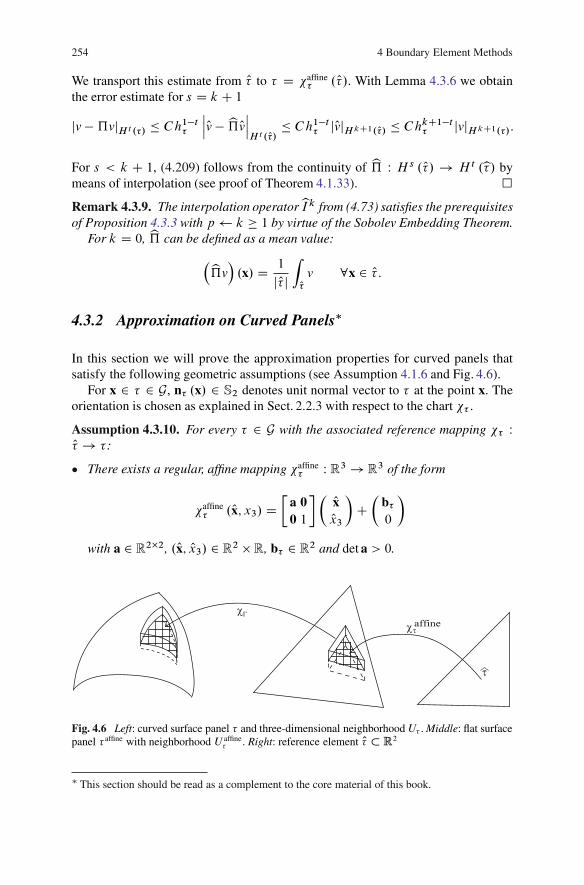
254 4 Boundary Element Methods
We transport this estimate from O� to � D �affine� . O�/. With Lemma 4.3.6 we obtain
the error estimate for s D k C 1jv �…vjH t .�/ � Ch1�t�
ˇˇOv � b…Ov
ˇˇH t . O�/ � Ch
1�t� jOvjHkC1. O�/ � ChkC1�t� jvjHkC1.�/:
For s < k C 1, (4.209) follows from the continuity of b… W H s . O�/ ! H t .b�/ bymeans of interpolation (see proof of Theorem 4.1.33). �Remark 4.3.9. The interpolation operatorbI k from (4.73) satisfies the prerequisitesof Proposition 4.3.3 with p k � 1 by virtue of the Sobolev Embedding Theorem.
For k D 0, b… can be defined as a mean value:
�b…v�.x/ D 1
j O� jZO�
v 8x 2 O�:
4.3.2 Approximation on Curved Panels
In this section we will prove the approximation properties for curved panels thatsatisfy the following geometric assumptions (see Assumption 4.1.6 and Fig. 4.6).
For x 2 � 2 G, n� .x/ 2 S2 denotes unit normal vector to � at the point x. Theorientation is chosen as explained in Sect. 2.2.3 with respect to the chart �� .
Assumption 4.3.10. For every � 2 G with the associated reference mapping �� WO� ! �:
� There exists a regular, affine mapping �affine� W R3 ! R3 of the form
�affine� .Ox; x3/ D
�a 00 1
�� OxOx3�C�
b�0
�
with a 2 R2�2, .Ox; Ox3/ 2 R2 �R, b� 2 R2 and det a > 0.
Fig. 4.6 Left: curved surface panel � and three-dimensional neighborhood U� . Middle: flat surfacepanel � affine with neighborhood U affine
� . Right: reference element O� R2
� This section should be read as a complement to the core material of this book.
4.3 Proof of the Approximation Property 255
� There exists a C1-diffeomorphism � W U ! V that is independent of G, withopen sets U; V � R3 that satisfy
� affine" � U; � affine
" WD ˚�affine� .Ox; 0/ W Ox 2b�� � .�"; "/;
�" � V; �" WD fxC ˛n� .x/ W x 2 � , ˛ 2 .�"; "/g
for an " > 0 such that�� .Ox/ D � ı �affine
� .Ox; 0/ :� For every function u 2 H k .�/ with a constant extension
u? .xC ˛n� .x// D u .x/ (4.210)
we have@�u? ı � ı �affine
�
�=@ Ox3 D 0: (4.211)
A situation of this kind was introduced in Example 4.1.7 (also see [170, Chap. 2]).First we will prove a transformation formula for composite functions.
Lemma 4.3.11. Let � W U ! V be a C1-diffeomorphism and let U; V � R3 beopen sets. For a function u 2 H k .V / we set Qu D u ı �. Then Qu 2 H k .U / and forall ˛ 2 N3
0 , 1 � j˛j � k, we have
.@˛ Qu/ ı ��1 Dj˛jXjˇ jD1
cˇ@ˇu (4.212)
with coefficients cˇ that are real linear combinations of products of the form
jˇ jYrD1
@�r�nr: (4.213)
The relevant indices for 1 � r � jˇj satisfy the relations 1 � nr � 3, r 2 N30 andPjˇ j
rD1 jr j D j˛j.Proof. For the equivalence u 2 H k .V / ” Qu 2 H k .U / it suffices to prove(4.212) for smooth functions. We will prove Formula (4.212) by induction. Let ekbe the k-th canonical unit vector in R3.
Initial case: For j˛j D 1 we obtain explicitly
.@˛ Qu/ ı ��1 DXjˇ jD1
cˇ@ˇu; where for ˇ D ek we have cˇ D @˛�k :
Hypothesis: Let the statement hold for j˛j � i � 1.
256 4 Boundary Element Methods
Conclusion: Let j˛j D i , choose k D 1; 2, or 3, and let Q D ˛ � ek 2 N30 . Thus
we obtain
.@˛ Qu/ ı ��1 D @k�@ Q Qu
�ı ��1 D
0@@k
i�1Xjˇ jD1
cˇ
�@ˇu
�ı �1A ı ��1
Di�1Xjˇ jD1
�@kcˇ
�@ˇuC
i�1Xjˇ jD1
3XjD1
�cˇ@k�j
� �@j @
ˇu�:
This proves the assertion if we show that @kcˇ and cˇ�@k�j
�are of the form
(4.213). With the Leibniz product rule we obtain
@k
jˇ jYrD1
@�r�nrDjˇ jXjD1
.@k@�j / �nj
jˇ jYrD1r¤j
@�r�nr
and the expression on the right-hand side is a linear combination of terms of theform
jˇ jYrD1
@ Q�r�nr
withPjˇ jrD1 j Qr j D i . The assertion follows analogously for the product cˇ
�@k�j
�.
�
Corollary 4.3.12. 1. Let the conditions of Lemma 4.3.11 be satisfied. Then
C�11 kQukL2.U / � kukL2.V / � C2 kQukL2.U /
and
jQuj2Hk.U /
� C1kXiD1juj2H i .V /
and juj2Hk.V /
� C2kXiD1jQuj2H i .U /
:
The constants C1; C2 depend only on k and the derivatives of �, ��1 up to theorder max f1; kg.
2. Let Assumption 4.3.10 and the conditions of Lemma 4.3.11 be satisfied with � �. For � 2 G, � affine WD ��1 .�/ and u 2 H k .�/, Qu .Ox/ WD u ı � .Ox; 0/ we have
C�13 kQuk2L2.�affine/ � kuk2L2.�/� C4 kQuk2L2.�affine/
4.3 Proof of the Approximation Property 257
and
jQuj2Hk.�affine/ � C3
kXiD1juj2H i .�/
and juj2Hk.�/
� C4kXiD1jQuj2H i.�affine/ :
The constants C3; C4 again depend only on k and the derivatives of �, ��1 up tothe order k.
Proof. Statement 1 follows from the transformation formula (4.212).For the second statement we define a constant extension of u in the direction of
the normal as a function u?, according to (4.210), and note that the normal derivativeof u? vanishes, i.e., we have ju?jHk.�"/
D jujHk .�/.From (4.211) we have ju? ı �jHk.�affine
" / D jQujHk.�affine/ and, thus, we have theassertion in Part 1. �
At the next step we will apply Lemma 4.3.11 to the composite reference mappingand study how far this depends on the panel diameter h� .
Lemma 4.3.13. Let Assumption 4.3.10 and the conditions of Lemma 4.3.11 holdwith � �. For � 2 G and u 2 H k .�/, � � V , Ou WD u ı �� we have
v 2 H k.�/”Ov WD v ı �� 2 H k. O�/ (4.214)
and
juj2Hk.�/
� C1h2�2k�
kXiD1jOuj2H i .O�/ ; (4.215a)
jOuj2Hk. O�/ � C2h2k�2�
kXiD1juj2H i .�/
: (4.215b)
The constants C1, C2 depend only on k, the constant �G of the shape-regularity (seeDefinition 4.1.12) and the derivatives �, ��1 up to the order k.
Proof. It follows from Corollary 4.3.12 that
juj2Hk .�/� C
kXiD1jQuj2H i.�affine/ :
We can therefore apply the transformation formulas from Lemma 4.3.6, which givesus the estimates
258 4 Boundary Element Methods
juj2Hk.�/
� C1h2�kXiD1
h�2i jQuj2H i.�affine/ � C2h2�2k�
kXiD1jOuj2H i . O�/ ;
jOuj2Hk.O�/ � C3h2k�2� jQuj2Hk.�affine/ � C4h2k�2�
kXiD1juj2H i .�/
:
�With this we obtain the analogy of Theorem 4.3.8 for curved panels.
Theorem 4.3.14. Let Assumption 4.3.10 and the conditions from Lemma 4.3.11hold with � �. Let � 2 G be the image of the reference element O� as givenby � D � ı �affine
� . O�/. Let the interpolation operator b… W H s. O�/ ! H t . O�/ satisfythe conditions from Theorem 4.3.8 for 0 � t � s � k C 1.
Then we have for the operator… W H s.�/! H t .�/, which is defined by
…v WD�b…Ov� ı ��1� with Ov WD v ı �� ;
the error estimate for 0 � t � s � k C 1
8v 2 H kC1.�/ W jv �…vjH t .�/ � Chs�t� kvkH s.�/ : (4.216)
The constant C depends only on k, the shape-regularity of the surface mesh via theconstant �G in Definition 4.1.12 and the derivatives of �, ��1 up to the order k.
Theorem 4.3.8 and Theorem 4.3.14 contain the central, local approximationproperties that are combined in Sects. 4.3.4 and 4.3.5 to form error estimates forboundary elements. The easiest way of constructing a global approximation forcontinuous boundary elements and sufficiently smooth functions is by means ofinterpolation. For this the functions u 2 H s
pw .�/ need to be continuous. In thefollowing section we will show that this is the case for s > 1.
4.3.3 Continuity of Functions in Hspw.�/ for s > 1
In order to avoid technical difficulties, we will generally assume in this section thatwe are dealing with the geometric situation from Example 4.1.7(1).
Assumption 4.3.15. � is a piecewise smooth Lipschitz surface that can be para-metrized bi-Lipschitz continuously over a polyhedral surface O�: �� W O� ! � .
Then the Sobolev spaces H s.�/ on � are defined invariantly for jsj � 1, whichmeans that they do not depend on the chosen parametrization of � (see Proposi-tion 2.4.2). For a higher differentiation index s > 1,H s
pw .�/ is defined as in (4.86).These spaces form a scale with
4.3 Proof of the Approximation Property 259
L2.�/ D H 0pw.�/ � H s
pw.�/ � H tpw.�/; 0 < s < t: (4.217)
Lemma 4.3.16. For s > 1 every u 2 H spw.�/ is continuous on � , i.e., H s
pw.�/ �C 0.�/.
Proof. � is the bi-Lipschitz continuous image of a polyhedral surface: � D ��� O��
and therefore it suffices to prove the statement for polyhedral surfaces. Let O�j , 1 �j � J , be the plane, relatively closed polygonal faces of the polyhedron.
Let u 2 H spw
� O�� for s > 1. The Sobolev Embedding Theorem implies that
u 2 C 0� O�j� for all 1 � j � J and, thus, it suffices to prove the continuity across
the common edges of the surface pieces O�j . For this we consider two pieces O�i andO�j with a common edge bE . Then there exists an (open) polygonal domain U � R2
and a bi-Lipschitz continuous mapping � W U ! O�i [ O�j with the properties
U 1 WD ��1� O�i
�; U 2 WD ��1
� O�j�; and �jUk
is affine for k D 1; 2:U1, U2 are disjoint and U D U1 [ U2:e WD ��1
�bE� D U1 \ U2:We only need to show that w WD u ı � is continuous over e. Clearly, we havewk WD w ı �k 2 H s .Uk/, k D 1; 2, and w 2 H 1 .U /. If we combine this resultwith the statements from Theorem 2.6.8 and Remark 2.6.10 we obtain the assertion.
�
4.3.4 Approximation Properties of Sp;�1G
We will now prove the error estimate (4.59) for the following two geometricsituations.
Assumption 4.3.17 (Polyhedral Surface). � is the surface of a polyhedron. Themesh G on � consists of plane panels with straight edges with mesh width h > 0:
Assumption 4.3.18 (Curved Surface). Assumption 4.3.10 holds and the condi-tions from Lemma 4.3.11 are satisfied with � �.
Theorem 4.3.19. Let either Assumption 4.3.17 or Assumption 4.3.18 hold. Lets � 0. Then there exists an operator Ip;�1G W H s
pw .�/! Sp;�1G such that
u � Ip;�1G uL2.�/
� C hmin.pC1;s/ kukH s.�/ : (4.218)
For a polyhedral surface the constantC depends only on p and the shape-regularityof the mesh G via the constant �G from Definition 4.1.12. In the case of a curved
260 4 Boundary Element Methods
surface it also depends on the derivatives of the global transformations �, ��1 upto the order k.
Proof. Let b…p
O� W H s . O�/! P�p be the L2-projection:
�b…p
O� u; q�L2.O�/ D .u; q/L2
�b�� 8q 2 P�p : (4.219)
We lift this projection to the panels � 2 G by means of
�…p� u�
�.x/ WD
�b…p
O� Ou��ı ��1� .x/ 8x 2 �;
where u� WD uj� and Ou� WD u� ı �� . The operator Ip;�1G then consists of thepanelwise composition of …p
� :
Ip;�1G u
ˇˇ�WD …p
� u 8� 2 G:
Obviously, this defines a mapping fromH spw .�/ to Sp;�1G . The operator b…p
O� satisfiesthe prerequisites of Theorem 4.3.8, because we have for the orthogonal projection:
1.b…p
O� Ov0� kOvk0 8Ov 2 L2 . O�/ :
Since b…p
O� Ov is a polynomial in a finite-dimensional space P�p , all norms are equiv-alent and there exists a constant Cp > 0 such that for all 0 � t � s � p C 1 wehave
b…p
O� Ovs� Cp
b…p
O� Ov0� Cp kOvk0 � Cp kOvkt 8Ov 2 H s . O�/ :
2. It follows immediately from the characterization (4.219) that
b…q D q 8q 2 P�p :
Therefore we can apply (4.209) or (4.216) with t D 0 and obtain the errorestimate ˇ
ˇv � Ip;�1G vˇˇL2.�/
� Chs� kvkH s.�/ (4.220)
for all v 2 H s .�/ with 0 � s � p C 1. If we then square and sum over all � 2 Gwe obtain the assertion. �
Theorem 4.3.19 gives us error estimates in negative norms by means of thesame duality argument as in the proof of Theorem 4.1.33. This is the subject ofthe following theorem.
Theorem 4.3.20. Let the assumption from Theorem 4.3.19 be satisfied. Then wehave for the interpolation Ip;�1G and 0 � t � s � p C 1 and all u 2 H s
pw .�/ theestimate
ku � Ip;�1G ukH�t .�/ � ChsCtkukH s.�/: (4.221)
4.3 Proof of the Approximation Property 261
Proof. The continuous extension of the L2 inner-product to H�tpw .�/ �H tpw .�/ is
again denoted by .�; �/0. Since Ip;�1G consists locally of L2-orthogonal projections,
we have for an arbitrary 'G 2 Sp;�1G
u � Ip;�1G uH�t .�/
D sup'2H t .�/nf0g
ˇˇ�
u � Ip;�1G u; '�0
ˇˇ
k'kH t .�/
D sup'2H t .�/nf0g
ˇˇ�
u � Ip;�1G u; ' � 'G�0
ˇˇ
k'kH t .�/
(4.222)
(see proof of Theorem 4.1.33). If we choose 'G D Ip;�1G ' 2 Sp;�1G , (4.221) followsby means of a twofold application of (4.218). �
Remark 4.3.21. Corollary 4.1.34 follows from (4.221) with t D 12
.
4.3.5 Approximation Properties of Sp;0G
Here we will prove approximation properties of continuous boundary elements thathave already been introduced in Proposition 4.1.50.
Theorem 4.3.22. Let Assumption 4.3.17 or Assumption 4.3.18 hold:
(a) Then there exists an interpolation operator Ip;0G W H spw.�/! S
p;0G such that
u � Ip;0G uH t .�/
� Chs�t kukH spw.�/
(4.223)
for t D 0; 1, 1 < s � p C 1 and all u 2 H spw .�/. For a polyhedral surface
the constant C depends only on p and on the shape-regularity of the mesh Gvia the constant �G from Definition 4.1.12. In the case of a curved surface italso depends on the derivatives of the global transformations �, ��1 up to theorder k.
(b) Let u 2 H s .�/ for some 1 < s � p C 1. Then, for any 0 � t � 1, we have
u � Ip;0G uH t .�/
� Chs�t kukH s.�/ :
Proof. Part a: Lemma 4.3.16 implies that u 2 H spw.�/ � C 0 .�/ for s > 1. We
define Ip;0G u on � 2 G by
�Ip;0G u�
�.x/ WD
�bIp Ou��ı ��1� .x/ 8x 2 � (4.224)
262 4 Boundary Element Methods
with u� WD uj� , Ou� WD u� ı �� and the interpolation operator bIp from (4.73) forthe set of nodal points †p from Theorem 4.1.39. By Theorem 4.1.39 this operatoris well defined and satisfies
�bIp Ou��.z/ D Ou� .z/ 8z 2 †p;
bIpq D q 8q 2 P O�p:
By Lemma 4.3.1 we have on the reference element
bIp Ou�H t .O�/ �
bIp Ou�HpC1.O�/ � c2
ˇˇbIp Ou�
ˇˇHpC1.O�/ C
Xz2†p
ˇˇ�bIp Ou�
�.z/ˇˇ!
D c2X
z2†p
jOu .z/j
� c2 kOukC0. O�/ � Cc2 kOukH s.O�/ :
Therefore Theorem 4.3.8 or Theorem 4.3.14 is applicable and for 1 < s � p C 1and t 2 f0; 1g we obtain the estimate
8u 2 H s.�/ Wˇˇu� � Ip;0G u�
ˇˇH t .�/
� Chs�t� ku�kH s.�/ : (4.225)
If we square (4.225) and sum over all � 2 Gaffine we obtain (4.223).Part b: By using Lemma 4.1.49 we derive from Part a the estimate
u � Ip;0G uH t .�/
� Chs�t kukH s.�/ (4.226)
for t 2 f0; 1g. We apply Proposition 2.1.62 with T D I �Ip;0G , Y0 D Y1 D H s .�/,X0 D L2 .�/, X1 D H 1 .�/, and � D t 2 .0; 1/ to interpolate the inequality(4.226). The result is
kT kH t .�/ H s.�/ � kT k1�tL2.�/ H s.�/ kT ktH1.�/ H s.�/
� �ChsG�1�t �Chs�1G�t D Chs�tG
and this implies the assertion of Part b. �
Next we investigate the approximation property for functions in H spw .�/ for
0 � s � 1. Recall that H spw .�/ D H s .�/ in this case. In general, functions in
H s .�/ are not continuous and the application of the pointwise interpolation Ip;0G isnot defined. We will introduce the Clement interpolation operator QG W L1 .�/!S1;0G for the approximation of functions in H s .�/ if 0 � s � 1 (cf. [69]). To avoid
technicalities, we consider only the case that all panels are (possibly curved) sur-face triangles. Let I denote the set of panel vertices with corresponding continuous,
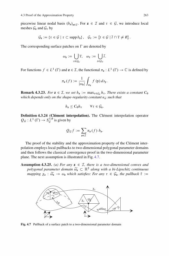
4.3 Proof of the Approximation Property 263
piecewise linear nodal basis .bz/z2I . For z 2 I and � 2 G, we introduce localmeshes Gz and G� by
Gz WD f� 2 G j � � supp bzg , G� WD˚t 2 G j t \ � ¤ ;� :
The corresponding surface patches on � are denoted by
!z WD[�2Gz
� , !� WD[t2G�
t :
For functions f 2 L1 .�/ and z 2 I, the functional �z W L1 .�/! C is defined by
�z .f / WD 1
j!zjZ!z
f .y/ dsy:
Remark 4.3.23. For z 2 I, we set hz WD max�2Gz h� . There exists a constant C0which depends only on the shape-regularity constant �G such that
hz � C0h� 8� 2 Gz:
Definition 4.3.24 (Clement interpolation). The Clement interpolation operatorQG W L1 .�/! S
1;0G is given by
QGf WDXz2I
�z .f / bz:
The proof of the stability and the approximation property of the Clement inter-polation employs local pullbacks to two-dimensional polygonal parameter domainsand then follows the classical convergence proof in the two-dimensional parameterplane. The next assumption is illustrated in Fig. 4.7.
Assumption 4.3.25. (a) For any z 2 I, there is a two-dimensional convex andpolygonal parameter domain e!z � R2 along with a bi-Lipschitz continuousmapping �z W e!z ! !z which satisfies: For any � 2 Gz, the pullback Q� WD
Fig. 4.7 Pullback of a surface patch to a two-dimensional parameter domain
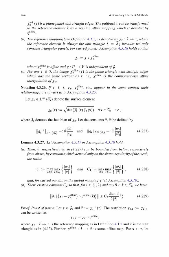
264 4 Boundary Element Methods
��1z .�/ is a plane panel with straight edges. The pullback Q� can be transformedto the reference element O� by a regular, affine mapping which is denoted by�affine.
(b) The reference mapping (see Definition 4.1.2) is denoted by �� W O� ! � , wherethe reference element is always the unit triangle O� D bS2 because we onlyconsider triangular panels. For curved panels, Assumption 4.3.18 holds so that
�� D � ı �affine�
where �affine� is affine and � W U ! V is independent of G.
(c) For any � 2 G, the image �affine� . O�/ is the plane triangle with straight edges
which has the same vertices as � , i.e., �affine� is the componentwise affine
interpolation of �� .
Notation 4.3.26. If � , Q� , O� , �� , �affine� , etc., appear in the same context their
relationships are always as in Assumption 4.3.25.
Let gz 2 L1 .e!z/ denote the surface element
gz .x/ WDq
det�J|
z .x/ Jz .x/� 8x 2 e!z a.e.,
where Jz denotes the Jacobian of �z. Let the constants �;‚ be defined by
g�1z
L1.e!z/
DW � je!zjj!zj and kgzkL1. Q!z/
DW ‚ j!zjje!zj : (4.227)
Lemma 4.3.27. Let Assumption 4.3.17 or Assumption 4.3.18 hold:
(a) Then, � , respectively ‚, in (4.227) can be bounded from below, respectivelyfrom above, by constants which depend only on the shape-regularity of the mesh,the ratios
c1 WD maxz2I max
�2Gz
j!zjj� j
�and C1 WD max
z2I max�2Gz
j Q!zjj Q� j
�; (4.228)
and, for curved panels, on the global mapping � (cf. Assumption 4.3.10).(b) There exists a constant C2 so that, for i 2 f1; 2g and any Qx 2 Q� � e!z, we have
@i ˚��� � �affine�
� ı �affine .Qx/� � C2 diam Q�2 j Q� j h
2� : (4.229)
Proof. Proof of part a. Let � 2 Gz and Q� WD ��1z .�/. The restriction �z;� WD �zjQ�can be written as
�z;� D �� ı �affine;
where �� W O� ! � is the reference mapping as in Definition 4.1.2 and O� is the unittriangle as in (4.13). Further, �affine W Q� ! O� is some affine map. For x 2 � , let
4.3 Proof of the Approximation Property 265
Ox WD ��1� .x/ and Qx WD ��affine��1
.Ox/. Then
Jz;� .Qx/ D J� .Ox/ Jaffine .Qx/ ; (4.230)
where Jz;� , J� , Jaffine are the Jacobi matrices of �z;� , �� , �affine, and
gz .Qx/ Dq
det�J|
affine .Qx/G� .Ox/ Jaffine .Qx/�
with G� .Ox/ WD J|� .Ox/ J� .Ox/ :
We introduce Gaffine WD J|affineJaffine and employ the multiplication theorem for
determinants to obtain
gz .Qx/ D jdet Jaffinejp
det G� .Ox/ Dp
det G� .Ox/2 j Q� j : (4.231)
If � is a plane triangle with straight edges then
pdet G� .Ox/ D 2 j� j :
For curved panels, we have �� D � ı �affine� (cf. Assumption 4.3.10) and obtain by
arguing as in (4.231)
c�2ˇ� affine
ˇ � pdet G� .Ox/ � C�2ˇ� affine
ˇwith � affine WD �affine
� . O�/ ;
where the constants 0 < c� � C� depend only on �, i.e., are independent of thediscretization parameters. From this we derive, by using the bi-Lipschitz continuityof � and the shape-regularity of the surface mesh, the estimate
2cc� j� j � 2c�h2� �p
det G� .Ox/ � 2C�h2� � 2CC� j� j ;
where c; C depend only on the shape-regularity constant �G . Thus
cc�
c1
j!zjje!zj � cc�
j� jj Q� j � jgz .Qx/j � CC� j� jj Q� j � CC�C1
j!zjje!zj :
Proof of part b. The statement is trivial for plane triangles with straight edgesbecause the left-hand side in (4.229) is zero.
Let z 2 I and assume that � 2 Gz is a curved panel. For any Qx 2 Q� � e!z, wehave
@i ˚��� � �affine�
� ı �affine .Qx/� �2XjD1
@j ��� � �affine�
�.Ox/ ˇ@i�affine
j .Qx/ˇ ;(4.232)
where Ox D �affine .Qx/ 2 O� .
266 4 Boundary Element Methods
Let cTp�� denote the p-th order Taylor expansion of �� about the barycenter bMof O� and let �affine
� D bI1�� be the affine interpolation at the vertices of O� . Then
����affine� D
��� � bT1��
�C�bT1�� � �affine
�
�D��� � bT1��
�CbI1
�bT1�� � ���:
For k D 0; 1, this splitting leads to the estimate
�� � �affine�
Ck. O�/ �
�1C
bI1Ck. O�/ Ck. O�/
��� � bT1��Ck. O�/
:
Standard error estimates for two-dimensional Taylor expansions result in
�� � bT1��C0. O�/
� 1
2max0�j�2
@j1@2�j2 ��
C0. O�/
:
Because @j bT1�� D bT0 �@j�� � we obtain
@j�� � @j bT1��C0. O�/
D@j�� � bT0@j��
C0. O�/
� max0�i�1
@i1@1�i2 @j��C0. O�/ :
Thus
�� � �affine�
Ck. O�/ �
�1C
bI1Ck. O�/ Ck. O�/
�max0�j�2
@j1@2�j2 ��
C0. O�/
:
(4.233)
Next, we will estimate the first factor in (4.233). For any w 2 C 0�O��
, we have
bI1wC0. O�/
D maxOx is a vertex of O�
jw .Ox/j � kwkC0.O�/ :
We denote the vertices of O� by bP 1 D .0; 0/, bP 2 D .1; 0/, bP 3 D .1; 1/ and thevalues of a continuous function w at bP j by wj , 1 � j � 3. It is easy to see that
@1bI1wC0. O�/
D jw2 � w1j � jw2 � w1jbP 2 � bP 1 � sup
Ox;Oy2O�jw .Ox/ � w .Oy/jkOx � Oyk � kwk
C1. O�/
and, similarly, we obtain the stability of the derivative @2. Hence we have provedthat the first factor in (4.233) is bounded from above by 2.
To estimate the second derivative of �� in (4.233) we write the mapping �affine� in
the form�affine� .Ox/ D B� OxC b�
with the (constant) Jacobi matrix B� 2 R3�2 and b� 2 R3. The columns of B� aredenoted by a1; a2 2 R3. As in the proof of Lemma 4.3.6, we use
4.3 Proof of the Approximation Property 267
@��� ı �affine
�
� D Xˇ2N3
0jˇ jD�1
X�2N3
0j�jD�2
Š
ˇŠ�Šaˇ1 a�2
�@ˇC��
�ı �affine
� :
Next, we employˇ.B� /i;j
ˇ � h� and obtain for any 2 N20 with jj D 2
supOx2O�
ˇ@��� ı �affine
�
�.Ox/ˇ � C3h2� ;
where C3 depends only on the derivatives of � which, by Assumption 4.3.10, areindependent of G. Thus we have proved that
�� � �affine�
Ck. O�/ � 2C3h2� (4.234)
and it remains to estimate the last factor in (4.232). Because �affine is affine, it isstraightforward to show that J�1affine 2 R2�2 [cf. (4.230)] has column vectors B � Aand C � B, where A, B, C denote the vertices of Q� . Hence
Jaffine D 1
2 j Q� j�.C � B/2 � .C � B/1� .B � A/2 .B �A/1
�:
Consequently ˇ@i�
affinej
ˇ � diam Q�2 j Q� j : (4.235)
�As a measure for the distortion of the local patches !z by the pullback, we
introduce the constant Cd by
Cd WD maxz2I
nje!zj�1=2 diam e!z
o: (4.236)
Theorem 4.3.28. Let Assumption 4.3.25 be satisfied.There exist two constants c1, c2 depending only on the shape-regularity constant
�G [cf. (4.17)], the constants Cd and C1 [as in (4.228)], and, for curved panels, onthe global chart � so that
kv �QGvkL2.�/ � c1h� kvkH1.!� /and kQGvkH1.�/ � Qc1 kvkH1.!� /
(4.237a)for all v 2 H 1 .�/ and all triangles � 2 G. Also,
kv �QGvkH� .�/ � c2hs��G kvkH s.�/ and kQGkH s.�/ H s.�/ � Qc2(4.237b)
for any 0 � � � s � 1 and v 2 H s .�/.
268 4 Boundary Element Methods
Proof. We present the proof in eight steps (a)–(h).
(a) For z 2 I, let �z W e!z ! !z be the mapping as in Assumption 4.3.25. For' 2 H 1 .!z/, the pullback to e!z is denoted by Q' WD ' ı �z. The Lipschitzcontinuity of �z implies that Q' 2 H 1 .e!z/.
We consider �z .'/ 2 C as a constant function and obtain
k' � �z .'/k2L2.!z/DZQ!z
gz .Qx/ j Q' .Qx/ � �z .'/j2 d Qx: (4.238)
Case 1: First, we consider the case of flat panels with straight edges. Note that, forany t 2 Gz and Qt WD ��1z .t/, we have gzjQt D jt j =
ˇeT ˇ.Let � 2 Gz. Then for any Qx 2 Q� D ��1z .�/
Q' .Qx/ � �z' D Q' .Qx/� 1
j!zjZ!z
' D Q' .Qx/� 1
j!zjZQ!z
gz Q'
D Q' .Qx/� 1
j!zjXt2Gz
ZQtgz Q' D Q' .Qx/� 1
j!zjXt2Gz
jt jˇeT ˇZQtQ' (4.239)
DXt2Gz
jt jj!zj . Q' .Qx/� �Qt Q'/
with �Qt Q' WD 1
jQtjRQt Q'. Applying the L2-norm to both sides yields
k Q' � �z'kL2.Q�/ �Xt2Gz
jt jj!zj k Q' � �Qt Q'kL2.Q�/ : (4.240)
Because eT � e!z are both convex we may apply Corollary 2.5.12 to obtain
k Q' � �Qt Q'kL2.Q�/ � k Q' � �Qt Q'kL2.e!z/ � 1C
sje!zjˇQt ˇ
!diam e!z
�j Q'jH1. Q!z/
��1C
pC1
� diam e!z
�j Q'jH1. Q!z/
; (4.241)
where C1 is as in (4.228). Inserting this into (4.240) yields
k Q' � �z'kL2.Q�/ ��1C
pC1
� diam e!z
�j Q'jH1. Q!z/
:
We sum over all Q� � e!z and apply a Cauchy–Schwarz inequality to derive theestimate
k Q' � �z'kL2. Q!z/�p
cardGz
�1C
pC1
� diam e!z
�j Q'jH1. Q!z/
;
4.3 Proof of the Approximation Property 269
where the number of panels .cardGz/ is bounded by a constant which depends onlyon the shape-regularity of the surface mesh.
The combination with (4.238) leads to
k' � �z .'/kL2.!z/�qkgzkL1. Q!z/
k Q' � �z'kL2. Q!z/
(4.227)� C4pj!zjdiam e!zpje!zj
j Q'jH1. Q!z/
� C4Cdhz j Q'jH1. Q!z/
with C4 WDp‚ cardGz
�1CpC1
�=� . From Lemma 4.3.6 resp. Lemma 4.3.13 we
obtainj Q'j2H1. Q!z/
DXQ�e!z
j Q'j2H1.Q�/ � C5X�2Gz
j'j2H1.�/(4.242)
and, finally, for any � � !z
k'��z .'/kL2.!z/�eC 6hz j'jH1.!z/
�C0eC 6h� j'jH1.!z/with eC 6 D CdC4
pC5:
(4.243)Case 2: Next, we consider the general case of curved panels. As in (4.239) we derive
Q' � �z' DXt2Gz
jt jj!zj
Q' � 1ˇeT ˇ
ZQt
ˇeT ˇjt j gz Q'
!
DXt2Gz
jt jj!zj
(. Q' � �Qt Q'/C
1ˇeT ˇZQtdt Q'
)(4.244)
with dt WD 1 � jeT jjt j gzjQt . The first difference in (4.244) can be estimated as in thecase of flat panels while, for the second one, we will derive an estimate of dt . Weuse the notation as in Assumption 4.3.25 and employ the splitting
dt D 1 �
ˇt affine
ˇjt j
!C 1
2 jt j�2ˇt affine
ˇ� 2 ˇeT ˇ .gzjQt /�; (4.245)
where t affine D �affinet . O�/ is the plane triangle with straight edges which interpolates
� at its vertices.We start by estimating the second term in (4.245). We employ the representation
(4.231) for Gram’s determinant to obtain
2ˇeT ˇ .gzjQt / D gt ;
where gt is Gram’s determinant of the reference map �t W O� ! t , i.e.
270 4 Boundary Element Methods
gt D k@1�t � @2�tk :
The area 2ˇt affine
ˇcan be expressed by
2ˇt affine
ˇ D @1�affinet � @2�affine
t
DW gaffinet (4.246)
Hence
ˇ2ˇt affine
ˇ� 2 ˇeT ˇ .gzjQt /ˇD ˇgaffine
t � gtˇD ˇ@1�affine
t � @2�affinet
�k@1�t � @2�tkˇ(4.247)
� @1�affinet � @2�affine
t � .@1�t � @2�t /
� @1 ��t � �affinet
� � @2�tC @1�affine
t � @2��t � �affine
t
� :We employ (4.234) to obtain
ˇ2ˇt affine
ˇ � 2 ˇeT ˇ .gzjQt /ˇ � 2C3h2t
�k@2�tkL1
�b�� C@1�affine
t
L1.O�/
�:
The estimate@1�affine
t
L1. O�/ � ht is obvious because t affine interpolates t in its
vertices. For the other term, we use
k@2�tkL1. O�/ D3XjD1
�@j� ı �affine
t
�@2��affinet
�j
L1. O�/
� Cht ;
whereC depends only on the global chart � but not on the discretization parameters.In summary we have proved that
ˇˇt affine
ˇ � ˇeT ˇ .gzjQt /ˇ
jt j � C3Cht
c;
where c depends only on the shape-regularity of the mesh and the global chart �.The first term of the sum in (4.245) can be estimated by using (4.247)
ˇˇˇ1 �
ˇt affine
ˇjt j
ˇˇˇ D
ˇˇˇjt j � ˇt affine
ˇjt j
ˇˇˇ � jt j�1
ZO�
ˇgt � gaffine
t
ˇdx
� C3Ch3t
jt j � C3Cht
c:
This finishes the estimate of dt
4.3 Proof of the Approximation Property 271
jdt j � 2C3Ccht :
Inserting this into (4.244) and proceeding as in the case of flat panels yields
k Q' � �z'kL2.Q�/ �Xt2Gz
jt jj!zj k Q' � �Qt Q'kL2.Q�/ C
Xt2Gz
jt jj!zj2
C3C
cht
sj Q� jˇeT ˇ k Q'kL2. QT /
(4.241)��1C
pC1
� diam e!z
�j Q'jH1. Q!z/
C 2C3CpC1
chz k Q'kL2. Q!z/
:
We sum over all Q� � e!z and apply a Cauchy–Schwarz inequality to derive theestimate
k Q' � �z'kL2. Q!z/�p
cardGz
( �1C
pC1
� diam e!z
�j Q'jH1. Q!z/
C 2C3CpC1
chz k Q'kL2. Q!z/
):
From Lemma 4.3.6 resp. Lemma 4.3.13 we obtain the scaling relations
j Q'j2H1. Q!z/�C5 j'j2H1.!z/
and Qc5 je!zjj!zj k'k
2L2.!z/
�k Q'k2L2. Q!z/�eC 5 je!zj
j!zj k'k2L2.!z/
and, finally, for any � � !z
k' � �z'kL2.!z/� bC 6hz k'kH1.!z/
� C0bC 6h� k'kH1.!z/; (4.248)
where bC 6 depends on C1, Cd, C5, Qc5, eC 5, and cardGz. Let C6 WD maxneC 6;bC 6
o[cf. (4.243)].
(b) Let � 2 G. The set of vertices of � is denoted by I� . Then
Xx2I�
bx D 1 on �:
By using Step a, we derive
k' �QG'kL2.�/ DXz2I�
bz .' � �z .'//
L2.�/
�Xz2I�
kbz .' � �z .'//kL2.�/
�Xz2I�
k' � �z .'/kL2.�/ �Xz2I�
k' � �z .'/kL2.!z/

272 4 Boundary Element Methods
� C0C6h�Xz2I�
k'kH1.!z/
� p3C0C6h�sX
z2I�
k'k2H1.!z/(4.249)
� p3C0C6h�sXt2!�
Xz2I� Wt!z
k'k2H1.t/
� C7h� k'kH1.!� /(4.250)
with C7 WD 3C0C6.(c) By summing over all panels we obtain
k' �QG'k2L2.�/DX�2Gk' �QG'k2L2.�/
� C 27 h2GX�2Gk'k2H1.!� /
D C 27 h2GXt2G
X�2GWt!�
k'k2H1.t/ � C 28 h2G k'k2H1.�/ ;
where C8 D C7C 1=2]and
C] WD maxt2G card f� 2 G W t � !� g
depends only on the shape-regularity constant.
(d) For the L2 .�/-stability we repeat the first steps of (4.249) to obtain
kQG'kL2.�/ �Xz2I�
k�z .'/kL2.!z/:
The Cauchy-Schwarz inequality yields
j�z .'/j � j!zj�1=2 k'kL2.!z/
and as in (4.250) we derive
kQG'kL2.�/ �Xz2I�
k'kL2.!z/� p3 k'kL2.!� /
: (4.251)
A summation as in Step c results in theL2 .�/-stability of the Clement interpolationoperator
kQG'kL2.�/ �p3C] k'kL2.�/ : (4.252)
4.3 Proof of the Approximation Property 273
(e) From Step c and Step d we conclude that
k' �QG'kL2.�/ � C9 k'kL2.�/ and k' �QG'kL2.�/ � C8hG k'kH1.�/
hold with C9 WD 1 C p3C]. Hence the approximation result for the intermedi-
ate Sobolev spaces H s .�/, s 2 �0; 1Œ, follows by interpolation as in the proof ofTheorem 4.1.33.
(f) For the local H 1-stability we proceed as in Step d, respectively as in (4.249).Recall the definition of the surface gradient as in (4.200) and (4.201) to derive
jQG'jH1.�/ DXz2I�
�z .'/rSbz
L2.�/
DXz2I�
��z .'/ � �z0
.'/�rSbz
L2.�/
(4.253)
for any fixed z0 2 I� . Let N'� WD 1j!� j
R!�'. Then �z . N'� / D �z0
. N'� / D N'� and
ˇ�z .'/ � �z0
.'/ˇ � j�z .'/ � �z . N'� /j C
ˇ�z0
. N'� /� �z0.'/ˇ
�ˇˇ 1j!zj
Z!z
.' � N'� /ˇˇC
ˇˇˇ1ˇ!z0
ˇZ!z0
. N'� � '/ˇˇˇ
� k' � N'�kL2.!z/
j!zj1=2Ck' � N'�kL2.!z0/ˇ
!z0
ˇ1=2 :
In a similar fashion to (4.243) and (4.248) one derives forD 2 ˚!z; !z0
�
k' � N'�kL2.D/ � k' � N'�kL2.!� /� eC 7 .diam!� / k'kH1.!� /
:
Hence ˇ�z .'/ � �z0
.'/ˇ � C10 k'kH1.!� /
; (4.254)
whereC10 depends only on the shape-regularity constant and the global parametriza-tion �.
In Theorem 4.4.2 (with ` D 1 and m D 0), we will prove the inverse inequalityand, thus, obtain the estimate
krSbzkL2.�/ � Ch�1� kbzkL2.�/ � Ch�1� j� j1=2 � C11; (4.255)
where C11 depends only on the shape-regularity of the mesh and the globalparametrization �.
By inserting (4.254) and (4.255) into (4.253) we derive
jQG'jH1.�/ � 3C10C11 k'kH1.!� /:
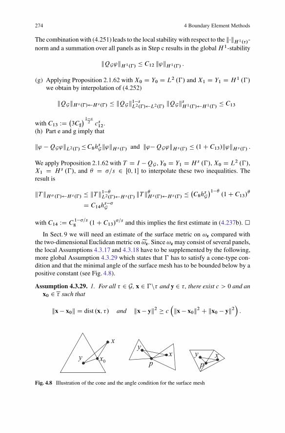
274 4 Boundary Element Methods
The combination with (4.251) leads to the local stability with respect to the k�kH1.�/-norm and a summation over all panels as in Step c results in the globalH 1-stability
kQG'kH1.�/ � C12 k'kH1.�/ :
(g) Applying Proposition 2.1.62 with X0 D Y0 D L2 .�/ and X1 D Y1 D H 1 .�/
we obtain by interpolation of (4.252)
kQGkH s.�/ H s.�/ � kQGk1�sL2.�/ L2.�/kQGksH1.�/ H1.�/
� C13
with C13 WD�3C]
� 1�s2 cs12.
(h) Part e and g imply that
k' �QG'kL2.�/�C8hsGk'kH s.�/ and k'�QG'kH s.�/ � .1C C13/k'kH s.�/ :
We apply Proposition 2.1.62 with T D I �QG , Y0 D Y1 D H s .�/, X0 D L2 .�/,X1 D H s .�/, and � D �=s 2 Œ0; 1� to interpolate these two inequalities. Theresult is
kT kH� .�/ H s.�/ � kT k1��L2.�/ H s.�/ kT k�H s.�/ H s.�/ ��C8h
sG�1��
.1C C13/�D C14hs��G
with C14 WD C 1��=s8 .1C C13/�=s and this implies the first estimate in (4.237b). �
In Sect. 9 we will need an estimate of the surface metric on !z compared withthe two-dimensional Euclidean metric on e!z. Since!z may consist of several panels,the local Assumptions 4.3.17 and 4.3.18 have to be supplemented by the following,more global Assumption 4.3.29 which states that � has to satisfy a cone-type con-dition and that the minimal angle of the surface mesh has to be bounded below by apositive constant (see Fig. 4.8).
Assumption 4.3.29. 1. For all � 2 G, x 2 �n� and y 2 � , there exist c > 0 and anx0 2 � such that
kx � x0k D dist .x; �/ and kx � yk2 � c�kx � x0k2 C kx0 � yk2
�:
Fig. 4.8 Illustration of the cone and the angle condition for the surface mesh
4.3 Proof of the Approximation Property 275
2. For all �; t 2 G whose intersection consists of at most one point, there exists apoint p of t such that
kx � yk � c .kx � pk C kp� yk/ 8x 2 �;8y 2 t:
3. For all �; t 2 G with exactly one common edge � \ t D E and for all x 2 � , y 2 tthere exists a point p 2 E such that
ky � xk � c .ky � pk C kp� xk/ :
Lemma 4.3.30. Let Assumption 4.3.29 be satisfied and let Assumption 4.3.17 orAssumption 4.3.18 hold. Then
c kQx � Qyk � diam e!z
hzk�z .Qx/ � �z .Qy/k � C kQx � Qyk 8Qx; Qy 2 e!z;
where C depends only on the global chart � but is independent of the surface mesh.
Proof. (a) Let � 2 Gz be a surface triangle with vertices A, B, C. First, we will provethe statement for Qx, Qy 2 Q� D ��1z .�/.
Let � affine WD �affine� . O�/ be the plane triangle with straight edges which interpo-
lates � in its vertices. Note that ��� affine
� D � . Hence
� .x/� � .y/ D J� .w/ .x � y/ 8x; y 2 � affine
where J� 2 R3�3 is the Jacobi matrix of the global chart � and w is some point inxy. Note that the largest and the smallest eigenvalues �max and �min of the positivedefinite Gram matrix G� depend only on the global chart � and are, in particular,independent of the discretization parameters. Thus
p�min kx � yk � k� .x/� � .y/k �
p�max kx � yk 8x; y 2 � affine:
Let Gaffine� 2 R2�2 denote the (constant) Gram matrix of �affine
� . From Lemma 4.3.5we conclude that
�affine� .Ox/ � �affine
� .Oy/ D ˝Gaffine� .Ox � Oy/ ; .Ox � Oy/˛1=2 � p2h� kOx � Oyk
for all Ox; Oy 2 O� . Because the matrix Gaffine� is symmetric and positive definite, its
minimal eigenvalue �affinemin can be expressed by
�affinemin D
�Gaffine�
��1�1 :We employ Lemma 4.3.5 to obtain
�affine� .Ox/ � �affine
� .Oy/ � ch� kOx � Oyk
276 4 Boundary Element Methods
for all Ox; Oy 2 O� , where C depends only on the shape-regularity of the mesh. Thuswe have proved that
cp�minh� kOx � Oyk � k�� .Ox/ � � .Oy/k �
p2�maxh� kOx � Oyk
for all Ox; Oy 2 O� . Finally, we replace Ox and Oy by �affine .Qx/ and �affine .Qy/. From (4.235)we derive the estimate for the largest eigenvalue �max
of the Gram matrix G of�affine q
�max
(4.235)� p2
diam Q�2 j Q� j � C diam�1 Q�;
where C depends only on the shape-regularity constant and the global chart �.For the smallest eigenvalue we use
G�1 D� kQe1k2 hQe1; Qe2ihQe1; Qe2i kQe2k2
�;
where eA;eB;eC denote the vertices of Q� and Qe1 D eB �eA, e2 D eC �eB. Thus
G�1 � 2 diam Q�
and the minimal eigenvalue �min satisfies
q�min D
G�1�1=2 � 1p
2 diam Q� :
The combination of these estimates leads to
ch�
diam Q� kQx � Qyk � k�z .Qx/� �z .Qy/k � C h�
diam Q� kQx � Qyk 8Qx; Qy 2 Q�:(4.256)
(b) We assume that Gz contains more than one panel and consider the case that xand y belong to different panels �; t 2 Gz. Note that
chz
diam e!z� h�
diam Q� � Chz
diam e!z8� 2 Gz;
where c and C depend only on the global chart � and the shape-regularityconstant. Assumption 4.3.29 implies that one of the following two cases issatisfied:
(i) The panels � and t share exactly one common edge � \ t D E . Then thereexists a point p 2 E such that
ky � xk � c .ky � pk C kp � xk/ :
4.3 Proof of the Approximation Property 277
The combination of (4.256) and a triangle inequality leads to
ky � xk � Qc hz
diam e!z.kQy � Qpk C kQp � Qxk/ � Qc hz
diam e!zkQy � Qxk
with Qp WD ��1z .p/. For the upper estimate we use QxQy � e!z since e!z isconvex. Let .epi /qiD0 be the minimal number of points lying on QxQy such that
Qp0 D Qx; Qpq D y; and 81 � i � q W Qpi�1 Qpi is contained in some Q� � e!z:
Let pi D �z . Qpi /, 1 � i < q. Then the upper estimate follows from
ky � xk�qXiD1kpi � pi�1k�C hz
diam e!z
qXiD1kQpi � Qpi�1k D C hz
diam e!zkQy � Qxk :
(ii) � and t share exactly one common point fzg D � \ t . Then
kx � yk � c .kx � zk C kz � yk/
and the rest of the proof is just a repetition of the arguments as in Case i. �
Lemma 4.3.31. Let Assumption 4.3.17 or Assumption 4.3.18 be satisfied. For � 2Gz, let �z;� WD �zjQ� , where Q� WD ��1z .�/. Then, for any 2 N2
0 with k WD jj,
k@��z;�kL1.Q�/ � C�
hz
diam e!z
�k;
where C depends only on k, C1 as in (4.228), Cd as in (4.236), and the globalchart �.
Proof. Recall that �z;� D � ı �affine, where �affine D �affine� ı �affine is affine. As in the
proof of Lemma 4.3.6, we use
@��� ı �affine� D X
ˇ2N20jˇ jD�1
X�2N2
0j�jD�2
Š
ˇŠ�Šaˇ1 a�2
�@ˇC��
�ı �affine;
where a1, a2 are the column vectors of the Jacobi matrix of �affine, that is,
.ai /j D @j �affinei D
2XkD1
@k�affine�;i @j �
affinej :
278 4 Boundary Element Methods
We haveˇˇ@k�affine
�;i
ˇˇ � h� and from (4.235) we conclude that
ˇˇ@i�affine
j
ˇˇ �
diam Q�= .2 j Q� j/. This leads toˇ.ai /j
ˇ � h� diam Q�= j Q� j. Thus
ˇ@��� ı �affine
�ˇ � C�h� diam Q�j Q� j
�k� C
�C1Cd
hz
diam e!z
�k;
where C depends only on k and the global chart �. �
4.4 Inverse Estimates
The spaces H s.�/ form a scale:
H s.�/ � H t .�/; for t � s (4.257)
with a continuous embedding: there exists some C.s; t/ > 0 such that
kukH t .�/ � C.s; t/ kukH s.�/ ; 8u 2 H s.�/: (4.258)
Note that the range of s and t may be bounded by the smoothness of the surface (seeSect. 2.4). In general, the inverse of this inequality is false.
Exercise 4.4.1. Find a sequence of functions .un/n2N 2 C1 .Œ0; 1�/ which contra-dicts the inverse of (4.258) for s D 0 and t D 1, i.e., which satisfies
limn!1 kunkH1.Œ0;1�/ = kunkL2.Œ0;1�/ D 1:
However, for boundary element functions there is a valid inverse of (4.258), aso-called inverse inequality, where the constant C depends on the dimension of theboundary element space. In the following we will assume that the maximal meshwidth h is bounded above by a global constant h0. For example, we can chooseh0 D diam� or otherwise h0 D 1 for sufficiently fine surface meshes. Recall thedefinition of P �
kas in (4.67):
Theorem 4.4.2. Let either Assumption 4.3.17 or Assumption 4.3.18 hold. We havefor 0 � m � `, all � 2 G and all v 2 P �
k:
kvkH`.�/ � Chm�`� kvkHm.�/ :
The constant C depends only on h0, `, k and, for a polyhedral surface, on theshape-regularity of the mesh G via the constant �G from Definition 4.1.12. In the caseof a curved surface it also depends on the derivatives of the global transformations�, ��1 up to the order k.
4.4 Inverse Estimates 279
Proof. Owing to the h-independent equivalence of the norms kvkH`.�/ andkQvkH`.�affine/ from Corollary 4.3.12, it suffices to consider the case of a planepolyhedral surface.Case 1: m D 0. Since P �
kis finite-dimensional, all norms on P �
kare equivalent:
There exists a positive constant C` such that for 0 � j � `
kOvkHj . O�/ � C` kOvkL2.O�/ 8Ov 2 P O�k :
With Lemma 4.3.6 or Lemma 4.3.13 it follows for all v 2 P �k
that
jvjHj .�/ � C1h1�j� jOvjHj . O�/ � C`C1h1�j� kOvkL2. O�/ � C`C1C2h�j� kvkL2.�/ :
For the k�kH` -norm, by summing the squares of the seminorm we obtain
kvkH`.�/ � Ch�`� kvkL2.�/ ; (4.259)
where C depends on `, k and the upper bound of the mesh width h0.Case 2: 0 < m � `. For ` �m � n � ` and j˛j D n we write @˛v D @ˇ@˛�ˇ withjˇj D ` �m and ˇ � ˛ componentwise. Then with Case 1 we have
k@˛vkL2.�/ �ˇˇ@˛�ˇ v
ˇˇH`�m.�/
� Chm�`�
@˛�ˇ vL2.�/
� Chm�`� jvjHn�`Cm.�/ :
Since j˛j D n was arbitrary, this result and n � `Cm � m together yield
jvjHn.�/ � Chm�`� jvjHn�`Cm.�/ � Chm�`� kvkHm.�/ (4.260)
for an arbitrary ` � m � n � `. (Note that the constant C in (4.260) depends onn;m; and `. However, n and m are from the finite set f0; 1; : : : ; `g and – by takingthe maximum over n and m – results in a constant C which does not depend onn and m but on ` instead.) Inequality (4.259) for ` ` � m as well as Estimate(4.260) finally yield the assertion
kvk2H`.�/
D kvk2H`�m.�/
CmX
nD`�mC1jvj2Hn.�/
� C8<:h2.m�`/� kvk2L2.�/
CmX
nD`�mC1h2.m�`/� kvk2Hm.�/
9=;
� Ch2.m�`/� kvk2Hm.�/ :
�
280 4 Boundary Element Methods
The global version of Theorem 4.4.2 requires the quasi-uniformity of the surfacemesh G.
Theorem 4.4.3. Let either Assumption 4.3.17 or Assumption 4.3.18 hold. Then wehave for all t; s 2 f0; 1g, t � s, the estimate
8v 2 Sp;0G W kvkH s.�/ � Cht�skvkH t .�/: (4.261)
The constant C depends only on h0, p and, for a polyhedral surface, on the shape-regularity and quasi-uniformity of the mesh G via the constants �G and qG fromDefinitions 4.1.12 and 4.1.13. In the case of a curved surface it also depends on thederivatives of the global transformations �, ��1 up to the order k.
Proof. From Theorem 4.4.2 we have
kvk2H s.�/ DX�2Gkvk2H s.�/ � C
X�2G
h2.t�s/� kvk2H t .�/ � C�
min�2G h�
�2.t�s/kvk2H t .�/
��Cq
2.s�t/G
�h2.t�s/ kvk2H t .�/ :
�Theorem 4.4.3 can be generalized in various ways. In the following we will cite
results from [75].
Remark 4.4.4. (a) Theorem 4.4.3 holds for all t; s 2 R with 0 � t � s � 1 or�1 � t � 0 ^ s D 0 (see [75, Theorems 4.1, 4.6]).
(b) Theorem 4.4.3 is valid for the space Sp;�1G for all t; s 2 R with t D 0 ^ 0 �s < 1=2 or �1 � t � 0 ^ s D 0 (see [75, Theorems 4.2, 4.6]).
We will also require estimates between different Lp-norms and discrete `p-norms for boundary element functions and, thus, we again start with a local result.Here we will always consider the situation where a Lagrange basis is chosen for P O�
k
on O� . † DnbPi W i 2 � O�k
odenotes the set of nodal points onb� . The Lagrange basis�bN i
�i2 O�
k
of P O�k
satisfies
bN i
�bPj�D ıi;j 8i; j 2 � O�k :
A vector of coefficients w WD .wi /i2 O�k
is put into relation with the associated
polynomial Ow 2 P O�k
on the reference element by means of
Ow WD bPw WDXi2 O�
k
wibN i :
4.4 Inverse Estimates 281
We define the “lifted” function
w WD P�w WDXi2 O�
k
wiNi with Ni D bN i ı ��1�
analogously.
Theorem 4.4.5. Let either Assumption 4.3.17 or Assumption 4.3.18 hold. For all� 2 G and all w WD .wi /i2 O�
k
we have
Qch� kwk`2 � kP�wkL2.�/ � eCh� kwk`2 :
The constants Qc and eC depend on the parameters qualitatively in the same way asdoes C in Theorem 4.4.3.
Proof. From Lemma 4.3.6 or Lemma 4.3.13 we have
ch� k OwkL2�b�� � kwkL2.�/ � Ch� k OwkL2
�b�� with Ow WD w ı �� :
Since all norms are equivalent on P O�k
, we have
ck k OwkHkC1. O�/ � k OwkL2. O�/ � Ck k OwkHkC1�b�� :
The equivalence of the H kC1 . O�/-norm and the Œ��kC1-norm follows from Lemma4.3.1. Since Ow 2 P O�
k,
Œ Ow�kC1 D j OwjHkC1.O�/CX
z2†k
j Ow .z/j DX
z2†k
j Ow .z/j DXi2 O�pjwi j D kwk`1 : (4.262)
Since ]†k is finite, there exist positive constants c; C depending only on thecardinality of †k , i.e., on k, such that
c kwk`2 � kwk`1 � C kwk`2 :
Combining all these results, we have thus proved that
Qch� kwk`2 � kwkL2.�/ � eCh� kwk`2 :
�
Corollary 4.4.6. Let the conditions from Theorem 4.4.5 be satisfied. Then
Och� kwkL1.�/ � kwkL2.�/ � bCh� kwkL1.�/

282 4 Boundary Element Methods
for all w 2 P �k
. The constants Oc;bC qualitatively depend on the parameters in thesame way as do Qc;eC in Theorem 4.4.3.
Proof. If we combine Theorem 4.4.5 with the norm equivalence on finite-dimensional spaces for w D .wi /i2 O�p and w D P�w it follows that
kwkL2.�/ � Ch� kwk`2 � bCh� kwk`1 � bCh� kwkL1.�/ :
Conversely, with the notation from the proof of Theorem 4.4.5 we have
kwkL1.�/ D k OwkL1.O�/ � C k OwkHkC1.O�/ � C 0 Œ Ow�kC1 (4.262)D C 0 kwk`1
� C 00 kwk`1 � C 000 kwk`2 :
Note that the constants in this estimate depend on the cardinality of †k , i.e., on k.From Theorem 4.4.5 we thus have the lower bound. �
The global version of Theorem 4.4.5 shows an equivalence between boundaryelement functions and the associated coefficient vector. Let .bi /
NiD1 be the Lagrange
basis of the boundary element space S . We define the operator P W RN ! S forw D .wi /NiD1 by
Pw DNXiD1
wibi :
Theorem 4.4.7. Let Assumption 4.3.17 or Assumption 4.3.18 hold. Then for allw 2 RN
Lch kwk`2 � kPwkL2.�/ � LCh kwk`2 :
The constants Lc; LC qualitatively depend on the parameters in the same way as Qc;eCdo in Theorem 4.4.5.
Proof. Let w 2 RN be the coefficient vector of the boundary element functionw D Pw. For � 2 G we can associate a global index ind .m; �/ 2 f1; 2; : : : ; N gon � with every local degree of freedom m 2 � O�
k. We set w� WD .w�;m/m2 O�
k
WD�wind.m;�/
�m2 O�
k
. With Theorem 4.4.5 we obtain
kPwk2L2.�/ DX�2GkP�wk2L2.�/ � Ch2
X�2Gkw�k2`2 :
The constant
M WD maxi2f1;2;:::;N g
]n.m; �/ 2 � O�p � G W i D ind .m; �/
o
4.4 Inverse Estimates 283
depends only on the polynomial degree k and on the shape-regularity of the surfacemesh. It thus follows that
kPwk2L2.�/� CMh2 kwk2`2 :
The lower bound can be found in a similar way. �
Corollary 4.4.8. Let either Assumption 4.3.17 or Assumption 4.3.18 hold and let.bi /i2I denote the nodal basis for the boundary element space S . Then
kbikL1.�/ � MC1: (4.263)
The constant MC1 depends only on the shape-regularity of the mesh and the polyno-mial degree of S .
If S D Sk;0G for some k � 1 then
jbi jW 1;1.�/ WD krSbikL1.�/ � MC2h�1� for any � � supp bi : (4.264)
The full W 1;1 .�/-norm is given by k�kW 1;1.�/ WD max˚k�kL1.�/ ; j�jW 1;1.�/
�and hence
kbikW 1;1.�/ � MC3h�1� for any � � suppbi : (4.265)
Proof. Let ei 2 RI denote the vector with .ei /i D 1 and .ei /j D 0 otherwise, i.e.,bi D P ei , Let � � supp bi . The combination of Corollary 4.4.6 and Theorem 4.4.5leads to
kbikL1.�/ � . Och� /�1 kbikL2.�/ � eC= Oc:Because bi j� D 0 for all � 2 Gi with � 6� suppbi we have proved (4.263).
For the proof of the second estimate we observe that – as in the proof of Theo-rem 4.4.3 – it suffices to consider plane panels with straight edges. Hence rSbi is apolynomial on every panel � so that
Och� krSbikL1.�/
Cor. 4.4.6� krSbikL2.�/
Theo. 4.4.2� Ch�1� kbikL2.�/
Theo. 4.4.5� CeC keik`2 D CeCfrom which the assertion follows. �
We can also analyze how far the constants in the norm equivalences depend onthe mesh width h in the case of the `p and Lp .�/-norms with 1 � p � 1. Herewe will only require the cases p D 2 and p D 1 and refer to [75] for the moregeneral case.
284 4 Boundary Element Methods
4.5 Condition of the System Matrices
One of the first applications of the inverse inequalities is the estimation of thecondition of the system matrices of the integral operators.
Lemma 4.5.1. Let Assumption 4.3.17 or Assumption 4.3.18 hold. Let K be the sys-tem matrix associated with the Galerkin discretization of the single layer operatorV for the Laplace problem. Then we have
cond2.K/ � Ch�1:
The constant C depends only on the polynomial degree p and the shape-regularityand the quasi-uniformity of the surface mesh G, more specifically on the constants�G and qG from Definitions 4.1.12 and 4.1.13. In the case of curved surfaces it alsodepends on the derivatives of the global transformations �, ��1 up to the order k.
Proof. Since K is symmetric and positive definite, we have
cond2.K/ D �max.K/�min.K/
:
In the following we will thus estimate the eigenvalues of K. It follows from thecontinuity and the H�1=2-ellipticity of the bilinear form .V �; �/0 W H�1=2 .�/ �H�1=2 .�/! K that there exist two positive constants � and Cc such that
� kuk2H�1=2.�/� .V u; u/0 � Cc kuk2H�1=2.�/
8u 2 H�1=2 .�/ :
From this it follows with Theorem 4.4.7 that
�max .K/ D maxwD.wi /i2RN nf0g
hKw;wikwk2 � Ch2 max
w2Snf0g.V w;w/0kwk2L2.�/
� Ch2Cc maxw2Snf0g
kwk2H�1=2.�/
kwk2L2.�/
� Ch2Cc:
By Theorem 4.4.7 and Remark 4.4.4 we have for the smallest eigenvalue
�min .K/ D minwD.wi /i2RN nf0g
hKw;wikwk2 � Ch2 min
w2Snf0g.V w;w/0kwk2L2.�/
� Ch2� minw2Snf0g
kwk2H�1=2.�/
kwk2L2.�/
� C 0h2�h:
Thus�max .K/ =�min .K/ � Ch�1
and the lemma follows. �

4.6 Bibliographical Remarks and Further Results 285
Exercise 4.5.2. Show that the system matrix K associated with the hypersingularoperator also satisfies the estimate
cond2 .K/ � Ch�1
under the conditions of Lemma 4.5.1.
Remark 4.5.3. For the condition of the mass matrix M WD��bi ; bj
�L2.�/
�Ni;jD1
we havecond2 .M/ � C:
Proof. Sincehw;Mwi D .Pw; Pw/L2.�/
we can apply Theorem 4.4.7:
Lc2h2 � minw2RN nf0g
hMw;wikwk2 � max
w2RN nf0ghMw;wikwk2 � LC 2h2;
from which we have the estimate of the condition with C D LC 2= Lc2. �
Estimating the condition of system matrices for equations of the second kind ismore problematic, as the stability of the Galerkin discretization for these equationsis in many cases still an open question. If we assume that the h-independent stabilityof the discrete operators is given, the condition of the system matrices for equationsof the second kind can be determined in terms of an h-independent constant in thesame way as before.
4.6 Bibliographical Remarks and Further Results
In the present chapter, we introduced spaces of piecewise polynomial functionson the boundary manifold � , and established approximation properties of thesespaces, as the meshwidth h tends to zero, in several function spaces of Sobolevtype on � . These boundary element spaces are, in a sense, Finite Element spaceson the boundary surface � . We also presented a general framework for the conver-gence analysis of Galerkin boundary element methods, in particular necessary andsufficient conditions for the quasi-optimality of the Galerkin solutions to hold.
For reasons of space, our presentation does not cover the most general cases.For example, the surface meshes upon which the boundary element spaces are builtdid not allow for local mesh refinement or, more importantly, for anisotropic localrefinements for example in the vicinity of edges (see, e.g., [75, 87, 234]).
Most of our results do extend to so-called graded, anisotropic meshes (cf. [104,107, 108]). In addition, besides mesh refinement, analogs of spectral methods or
286 4 Boundary Element Methods
even a combination of mesh refinement and order increase, the so-called hp-VersionBEM; is conceivable (cf. [222] and the references therein).
Further, for particular classes of boundary integral equations, special choices ofsubspaces may yield large gains in accuracy versus number of degrees of freedom.Let us mention, for example, the case of high frequency acoustic scattering. Here,the stability of the boundary integral operators depends, of course, on the problem’swave number but, in addition, also the solutions contain high-frequency compo-nents which are smooth, but highly oscillatory at large wave numbers, and thereforepoorly captured by standard boundary element spaces, unless the fine scale of theunknown functions on the boundary is resolved by sufficient mesh refinement. Thisstrategy may lead, however, to prohibitively large numbers of degrees of freedom.A better approach may be to augment the standard boundary element spaces byexplicitly known, dominant asymptotic components of the unknown solution. Inhigh frequency acoustics and electromagnetics, in particular for BIEs obtained fromthe direct method (where the unknowns are Cauchy data of the domain unknowns),strong results on the asymptotic structure of the solution are available from geo-metrical optics. These can be used to build boundary element spaces with no ora reduced preasymptotic convergence regime at high wave numbers. We refer e.g.to [5, 57, 153] for recent work on wave number independent Galerkin BEM foracoustics problems.
In this chapter, and throughout this book, we focused on Galerkin BEM. We doemphasize, however, that the alternative collocation BEM do constitute a powerfulcompetition; for collocation BEM on polyhedra, however, the theory of stability andquasi-optimality is much less mature that in the Galerkin case. Still, since colloca-tion methods do not require the numerical evaluation of double surface integrals,they offer a substantial gain in accuracy versus CPU time.
For this reason, in recent years substantial work has been devoted to collocationbased BIEs for high frequency acoustic and electromagnetic scattering. We mentionin particular the work of O. Bruno et al. (e.g. [34,35,161]) which is a collocation typeboundary element method which combines incorporation of high frequency asymp-totics with a degenerate coordinate transformation of the surface in the presence ofedges or vertices and a Nystrom type collocation procedure. The mathematical erroranalysis of this method is in progress.
The a priori asymptotic error bounds for Galerkin BEM developed in Sect. 4.2show that Galerkin BEM exhibit superconvergence in negative Sobolev norms on� . This allows us, in particular, to deduce corresponding results for postprocessedGalerkin approximations which can be obtained as smooth functionals of the solu-tion. Importantly, the insertion of the Galerkin solution into the representationformula is such a postprocessing operation. Therefore superconvergent pointwiseapproximations of the solution to the underlying boundary value problem at interiorpoints of the domain result usually from Galerkin boundary element approxi-mations. Note that our analysis in Sect. 4.2 reveals the crucial role of Galerkinorthogonality of the discretization in the derivation of superconvergence estimatesin negative order norms (indeed, for other discretization schemes such as colloca-tion or Nystrom methods, such superconvergence results either do not hold or only
4.6 Bibliographical Remarks and Further Results 287
with a much smaller gain in asymptotic convergence order). We finally note thatthe superconvergence error bounds for the solution at points x in the interior ofboth the domain � or its complement deteriorate as x approaches � . Nevertheless,this deterioration can be remedied and postprocessing procedures can be designedto recover superconvergent solution values and normal and tangential derivatives(required, for example, in shape optimization or uncertainty quantification) of arbi-trary order from the Galerkin solution such that the superconvergence bounds areuniform in the distance of x to the boundary � . For the details, we refer to [213].

http://www.springer.com/978-3-540-68092-5