the nature of fluid flow · viscosity quantiﬁes the resistance put up by a ﬂuid undergoing...

P1: PICc01 JWBK251-Ransing June 20, 2008 10:40 Printer Name: Yet to Come

1The Nature of Fluid Flow

Aim. To provide the reader with basic knowledge on the treatment of fluidat scales above and below the meso scale.

1.1 INTRODUCTION

The fundamentals of fluid flow on a wide range of scales are introduced in thischapter. The characterizing properties of a fluid and their relevance at large scales(kilometre to millimetre scale) and small scale (nanometre and angstrom scale)will be discussed. The continuum approach to describing the behaviour of a fluidwill be presented along with the methods of simulation at the continuum scale.In contrast, the molecular scale is considered along with fluid structure and sim-ulation methods used at this scale. Examples of the change in physics and fluidbehaviour that occur as the scale is reduced are presented, concentrating on theeffect of confinement on a fluid.

This chapter highlights the special requirements of meso scale systems. Ele-ments from both the continuum scale and the molecular scale are needed to modeland describe a meso scale fluid systemfully.

1.2 BASICS OF FLUID MOTION

The basic characteristic property that defines a fluid is viscosity. Fluid, unlikesolids, is unable to offer any permanent resistance to a shearing force. The fluidwill continue to deform as long as the force is applied, taking the shape of anysolid boundary it touches. The deformation of a fluid occurs from shearing forces

Fluid Properties at Nano/Meso Scale P. Dyson, R. S. Ransing, P. M. Williams and P. R. WilliamsC© 2008 John Wiley & Sons, Ltd

1

COPYRIG

HTED M

ATERIAL


2 THE NATURE OF FLUID FLOW

θ θ

Figure 1.1 Internal shear between fluid layers.

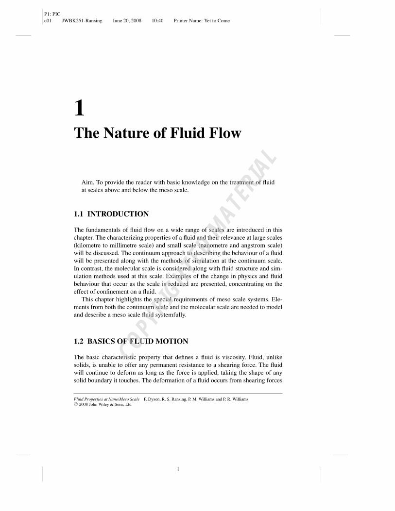
acting tangentially to any solid surface. The fluid can be considered as layersparallel to a surface, which slide over each other, as shown in Figure 1.1. Eachfluid layer applies a shear force to the next, and is in turn sheared by those ittouches.

The ability to deform continuously under an applied force makes fluids behavedifferently from solids. Solid bodies are capable of maintaining an unsupportedshape and structure, and can resist finite shear.

Fluids themselves fall into two categories, liquids and gases. To a fluid dynam-icist, who is interested in flows at the macro scale, there are two characterizingdifferences between them:

� Liquids have densities an order of magnitude larger than gases.� Liquids and gases respond very differently to changes in pressure and temper-

ature.

Gases can also be expanded and compressed more easily than liquids due to thelower density and spacing between molecules. The motion of all fluids relies onthe interaction and internal shear between fluid layers, but the actual interactionbetween layers occurs from collisions between many molecules on the molecularscale (∼ 10−9 m). In fact, all fluid effects and properties occur from molecularinteractions, but at the macro scale (∼ 10−4 m) the detailed molecular physics ofthis behaviour can be neglected as the number of molecules within the character-istic length can be considered as sufficiently large. At these scales the fluid can beviewed as having physical properties corresponding to the statistical averages ofthe underlying molecules and are known as continuum or bulk properties. Molec-ular physics, manifested in a continuum framework, has the ability to be definedas continuous functions of time and space.


BASICS OF FLUID MOTION 3

1.2.1 Continuum/Bulk Properties

Bulk or continuum properties such as velocity, density and pressure remain con-stant at a point and changes due to molecular motion are assumed to be negligible.These properties are also assumed to vary smoothly from point to point with nojumps or discontinuities. This assumption is correct as long as the characteris-tic distance of the system is of an order of magnitude greater than the distancebetween molecules.

This assumption of bulk physical properties allows the behaviour of fluid sys-tems to be approximated by a set of deterministic equations that represent theunderlying infinite chaotic molecular motion on a much larger scales. The defi-nition and basis of these bulk properties will be of significant importance in laterdiscussions, so it is necessary to explain the origin of some of these bulk proper-ties to clarify concepts.

1.2.1.1 Density

The density of a fluid is defined as the mass contained within a unit volume. It iscomputed as a function of mass (m) and volume (V ) of a sample as follows:

ρ = m

V. (1.1)

This expression of density is represented in terms of mass per unit volume(kg/m3). Other expressions of density used are specific weight (weight per unitvolume, N/m3), relative density (relative to another density, dimensionless) andspecific volume (reciprocal of density, m3/kg). Density can also be computed frommolecular properties, in terms of sample volume, V , containing N molecules ofindividual mass, mmolecule [3]:

ρ = Nmmolecule

V. (1.2)

This expression also has units of kg/m3 and can be defined from N = 1 toN = ∞.

1.2.1.2 Temperature

The temperature (T ) at any point in a fluid is derived from the internal kineticenergy of the underlying N molecules, each with velocity, vi , and mass, m [4]:

EKE =N∑

i=1

12 mv2

i . (1.3)



At continuum or bulk scales the number of molecules is assumed to be infinite,but the distribution of the velocity of this (almost) infinite number of moleculescan be assumed to follow the Boltzmann distribution, which in one dimensionappears as

f (v) =√

m

2πkbTe−mv2/2kbT , (1.4)

where kb is the Boltzmann constant. This distribution can then be used to calculatethe average squared velocity in the system to relate the velocity distribution to thekinetic energy,

〈v2〉 =√

m

2πkbT

∫ ∞

−∞v2e−mv2/2kbT dv, (1.5)

which gives

〈v2〉 =√

m

2πkbT

√π

2

(2kbT

m

)3/2

= kbT

m. (1.6)

The equation for the translational kinetic energy of the molecules can now berelated to the temperature of the system in one dimension:

EKE = 12 m〈v2〉 = kbT

2. (1.7)

For three dimensions, this simply becomes

12 m〈v2〉 = 3

2 NkbT, (1.8)

which describes the temperature of a local system of N molecules. In terms ofbulk properties, where locally N → ∞, the temperature is considered constantand varies smoothly from over the whole domain.

1.2.1.3 Pressure

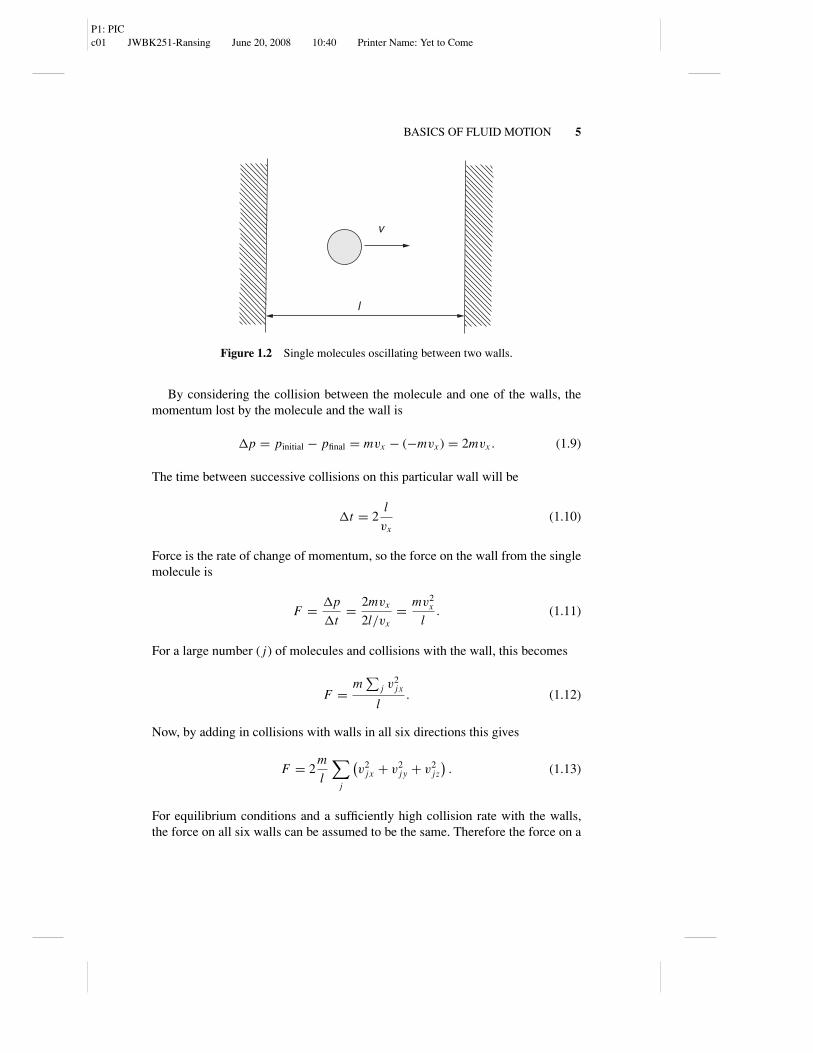
The pressure is explained by kinetic theory as arising from the force exerted bycolliding gas molecules on to the walls of the container [5]. To explain the me-chanics of pressure, consider a single molecule with velocity, v, along the x di-rection contained within two walls perpendicular to its direction of travel andseparated by length, l, as shown in Figure 1.2.



l

v

Figure 1.2 Single molecules oscillating between two walls.

By considering the collision between the molecule and one of the walls, themomentum lost by the molecule and the wall is

�p = pinitial − pfinal = mvx − (−mvx ) = 2mvx . (1.9)

The time between successive collisions on this particular wall will be

�t = 2l

vx(1.10)

Force is the rate of change of momentum, so the force on the wall from the singlemolecule is

F = �p

�t= 2mvx

2l/vx= mv2

x

l. (1.11)

For a large number ( j) of molecules and collisions with the wall, this becomes

F = m∑

j v2j x

l. (1.12)

Now, by adding in collisions with walls in all six directions this gives

F = 2m

l

∑j

(v2

j x + v2j y + v2

j z

). (1.13)

For equilibrium conditions and a sufficiently high collision rate with the walls,the force on all six walls can be assumed to be the same. Therefore the force on a



single wall becomes

F = 1

6

(2

m∑

j v2

l

)= m

∑j v2

3l, (1.14)

where v j is the velocity of molecule j in three dimensions. It is now possible totalk in terms of the average velocity of the molecules, (1/N )

∑j v2

j , which can be

represented by v2:

F = Nmv2

3l. (1.15)

This can then be divided by the area, A, of the wall to give the pressure

P = F

A= Nmv2

3l A. (1.16)

The cross-sectional area multiplied by length yields a volume, Al = V , whichwhen combined with Equation (1.2) yields

P = 13ρv2, (1.17)

thereby describing pressure as a function of density and kinetic energy ofmolecules, which, as shown in Equation (1.8), is in turn directly related to thetemperature of the system. As with temperature, at continuum scales the num-ber of molecules tends to infinity, and any fluctuations or statistical differencesbecome approximately zero. In this case both pressure and temperature may beconsidered as constant at any point in the fluid domain.

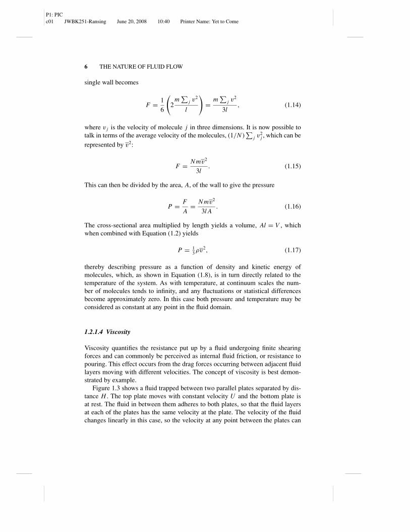
1.2.1.4 Viscosity

Viscosity quantifies the resistance put up by a fluid undergoing finite shearingforces and can commonly be perceived as internal fluid friction, or resistance topouring. This effect occurs from the drag forces occurring between adjacent fluidlayers moving with different velocities. The concept of viscosity is best demon-strated by example.

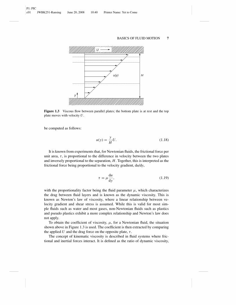
Figure 1.3 shows a fluid trapped between two parallel plates separated by dis-tance H . The top plate moves with constant velocity U and the bottom plate isat rest. The fluid in between them adheres to both plates, so that the fluid layersat each of the plates has the same velocity at the plate. The velocity of the fluidchanges linearly in this case, so the velocity at any point between the plates can



U

H u(y)

y

Figure 1.3 Viscous flow between parallel plates; the bottom plate is at rest and the topplate moves with velocity U .

be computed as follows:

u(y) = y

HU. (1.18)

It is known from experiments that, for Newtonian fluids, the frictional force perunit area, τ , is proportional to the difference in velocity between the two platesand inversely proportional to the separation, H . Together, this is interpreted as thefrictional force being proportional to the velocity gradient, du/dy,

τ = µdu

dy, (1.19)

with the proportionality factor being the fluid parameter µ, which characterizesthe drag between fluid layers and is known as the dynamic viscosity. This isknown as Newton’s law of viscosity, where a linear relationship between ve-locity gradient and shear stress is assumed. While this is valid for most sim-ple fluids such as water and most gases, non-Newtonian fluids such as plasticsand pseudo plastics exhibit a more complex relationship and Newton’s law doesnot apply.

To obtain the coefficient of viscosity, µ, for a Newtonian fluid, the situationshown above in Figure 1.3 is used. The coefficient is then extracted by comparingthe applied U and the drag force on the opposite plate, τ .

The concept of kinematic viscosity is described in fluid systems where fric-tional and inertial forces interact. It is defined as the ratio of dynamic viscosity,



µ, to the fluid density, ρ,

v = µ

ρ, (1.20)

Causes of viscosity Viscous effects occur due to internal friction between fluidlayers, and it is important to consider the nature and cause of this drag. Themolecules in a fluid are continuously moving and have little, if any, structure.Consequently, they are in constant molecular exchange between fluid layers. Thisexchange occurs via two mechanisms, the transfer of mass, by a fluid moleculephysically crossing between fluid layers, and the transfer of energy via interlayercollisions/potential energy interactions.

This constant exchange occurring over a sufficiently large number of collisionscauses energy and momentum to propagate smoothly throughout the fluid at arate governed by the physical properties of the molecular interactions and theconditions of the fluid. However, the condition of the fluid in terms of pressureand temperature causes different effects in liquids and gases.

Viscosity of gases In a gas, the molecules are widely spaced and interact rel-atively little, so an increase in temperature increases the kinetic energy of themolecules and viscosity increases as a result of increased mass transfer betweenlayers. According to the kinetic theory of gases [5], the viscosity is proportionalto the square root of the absolute temperature, This, however, is an exact solutionto an approximate model while in reality, the rate of increase of viscosity is muchhigher [3]. In gases, viscosity is found to be independent over the normal range ofpressures, with the exception of extremely high pressure.

Viscosity in liquids In liquids, which have much higher densities, the distancebetween molecules is much shorter and the cohesive/attractive forces betweenthem increase the viscous effect. The response to an increase in temperature, andhence kinetic energy, decreases the effect of these cohesive forces, which reducesthe viscosity. However, the increased molecular interchange between fluid lay-ers increases the viscosity [3]. The net result is that liquids show a reduction inviscosity for an increase in temperature.

Due to the close packing of the molecules in a liquid, high pressures also affectthe viscosity. At high pressures, the energy required for the relative movement ofa molecule is increased, causing an increase in viscosity.

1.2.2 Continuum Approximations

At distances above the micro scale, approximately ≥ 10−6 m, the number ofmolecules in the system can be in the order of millions! In these cases, the num-ber of molecular interactions occurring over length and time scales is also huge.Because of this, it can be considered acceptable to assume that the influence



of any individual molecular exchange/interaction is negligible as the number ofmolecules in any volume tends to infinity. The continuum assumption considersan infinite number of molecules in a domain and neglects their individual contri-butions. The interpretation of continuum is given as:

Continuum. A continuous thing, quantity, or substance; a continuous seriesof elements passing into each other [6].

If a fluid is considered as a continuum, then each part is considered as identical(i.e. the fluid is homogenous) to the next and infinitely divisible, and the molecularstructure of the fluid is ignored. This means that the fluid is assumed to have thesame properties even if the domain dimensions are 100 nm, 1 mm or 1 km.

By making the continuum assumption, molecular scale effects are neglectedand the bulk properties are defined by the physical observable relationships be-tween them. These properties can then be used to characterize fluid flows, as donein experiments by Reynolds [7] whose number, the Reynolds number, presents acriteria for dynamic similitude.

Re = ρuL

µ. (1.21)

The Reynolds number is the ratio of inertial (u/ρ) to viscous (µ/L) forces, whereL is the characteristic dimension of a flow with speed u. This can be used both todetermine kinematic and dynamic similitude for comparing scale models to realapplications and also to characterize the point of transition between laminar andturbulent flow (critical Reynolds number).

A large Reynolds number indicates that the inertial forces dominate the sys-tem, with a low viscosity causing the small scales of fluid motion to be relativelyundamped. A low Reynolds number flow, however, has high viscous forces, whichdamp out small scale motion.

The Reynolds number represents simple characterization of the behaviour ofa fluid system. To look more in depth at the measure and description of fluidbehaviour, a set of continuum governing equations is used. However, beforethese are considered it is important to set out the rules for the fluid mechan-ics interpretation of a continuum, which are known as the continuum assump-tions/approximations.

1.2.2.1 Continuum approximations

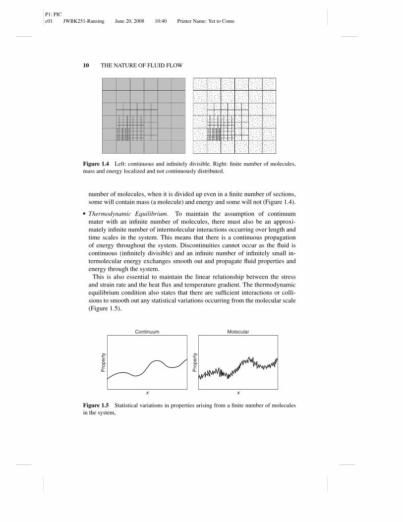
� Infinitely Divisible. The characteristic length of the fluid should be severalorders of magnitude larger than molecular diameters, such that the number ofmolecules in the system is large enough to be considered as approximately in-finite. By assuming an infinite number of molecules, the fluid is consideredhomogenous at all scales, and can be divided up/decomposed into an infinitenumber of identical sections. If the fluid is considered in terms of a finite



Figure 1.4 Left: continuous and infinitely divisible. Right: finite number of molecules,mass and energy localized and not continuously distributed.

number of molecules, when it is divided up even in a finite number of sections,some will contain mass (a molecule) and energy and some will not (Figure 1.4).

� Thermodynamic Equilibrium. To maintain the assumption of continuummater with an infinite number of molecules, there must also be an approxi-mately infinite number of intermolecular interactions occurring over length andtime scales in the system. This means that there is a continuous propagationof energy throughout the system. Discontinuities cannot occur as the fluid iscontinuous (infinitely divisible) and an infinite number of infinitely small in-termolecular energy exchanges smooth out and propagate fluid properties andenergy through the system.

This is also essential to maintain the linear relationship between the stressand strain rate and the heat flux and temperature gradient. The thermodynamicequilibrium condition also states that there are sufficient interactions or colli-sions to smooth out any statistical variations occurring from the molecular scale(Figure 1.5).

Molecular

Pro

pert

y

Continuum

Pro

pert

y

x x

Figure 1.5 Statistical variations in properties arising from a finite number of moleculesin the system,



If these conditions are met, the fluid system can be considered as a continuum.This is an important classification, as it means the flow can be approximated usingcontinuum laws.

The continuum laws can be applied in both simple analytical form, as in theBernoulli equation (inviscid flows),

P

ρ+ v2

2+ gh = constant, (1.22)

or for more complex situations that require numerical solution. For cases such assimple pipe flows, the Bernoulli equation can be of use where little informationis required. However, in complex systems or geometries, a more detailed analysisand interrogation is required. In this case, fluid behaviour can be simulated usinga set of conservative governing equations solved numerically. These simulations,based on the continuum assumptions and continuum scale observations and laws,provide a detailed and accurate model of fluid behaviour, where experiments aredifficult or expensive, or a greater amount of information is needed.

1.2.3 Continuum Scale Simulation

Both simple and complex fluid systems can be investigated, within the limits ofthe continuum assumptions, by sets of governing differential equations that de-scribe fluid behaviour. The mathematical solution of these equations throughouta fluid domain is known as computational fluid dynamics (CFD). The governingequations describe the mathematical representation of a physical model that isderived from experimental flow measurements and observations. These represen-tative equations are then replaced with an equivalent numerical description, whichis solved using numerical techniques for the dependent variables of velocity, den-sity, pressure and temperature. One of the most widely used sets of governingequations are the Navier–Stokes equations.

1.2.3.1 Navier–Stokes governing equations

The Navier–Stokes equations are a set of governing equations that describe thebehaviour of fluids in terms of continuous functions of space and time. Theystate that changes of momentum in the fluid are based on the product of the changein pressure and internal viscous dissipation forces acting internally. The schemeworks by not considering instantaneous values of the dependent variables, buttheir flux, which in mathematical terms is interpreted as the derivative of the vari-ables. The equation set is separated into three conservation laws for mass, energyand momentum.



Mass The conservation of mass, known as the continuity equation, is obtainedby considering the mass flux into and out of any elemental control volume withinthe flow field. In the Cartesian coordinate system, x , y, z, fluid velocities alongthose directions are u, v, w respectively. The continuity equation then becomes

δρ

δt+ δ(ρu)

δx+ δ(ρv)

δy+ δ(ρw)

δz= 0. (1.23)

The first term accounts for any change in density over time, while the rest of theterms describe the change in density in the x , y and z directions.

Energy The expression for the conservation of energy in a fluid system is

δ(ρe)

δt+ δ(ρue)

δx+ δ(ρve)

δy+ δ(ρwe)

δz

= ρQ + δ

δx

(kδT

δx

)+ δ

δy

(kδT

δy

)+ δ

δz

(kδT

δz

)

− P

(δu

δx+ δv

δy+ δw

δz

)− ϕ

(δu

δx+ δv

δy+ δw

δz

)2

+ µ

{2

[(δu

δx

)2

+(

δv

δy

)2

+(

δw

δz

)2]

+(

δv

δx+ δu

δy

)2

+(

δw

δy+ δv

δz

)2

+(

δu

δz+ δw

δx

)2}

, (1.24)

where ϕ is the bulk viscosity, Q is the heat added per unit mass, k is the thermalconductivity and e is the internal energy

Momentum The conservation of momentum equations are as follows:

δ(ρu)

δt+ δ(ρu2)

δx+ δ(ρuv)

δy+ δ(ρuw)

δz

= ρX − P

x+ δ

δx

{µ

[2δu

δx− 2

3

(δu

δx+ δv

δy+ δw

δz

)]}

+ δ

δy

[µ

(δu

δy

δv

δx

)]+ δ

δz

[µ

(δw

δx

δu

δz

)], (1.25)



δ(ρv)

δt+ δ(ρvu)

δx+ δ(ρv2)

δy+ δ(ρvw)

δz

= ρY − P

y+ δ

δy

{µ

[2δv

δy− 2

3

(δu

δx+ δv

δy+ δw

δz

)]}

+ δ

δz

[µ

(δv

δz

δw

δy

)]+ δ

δx

[µ

(δu

δy

δv

δx

)], (1.26)

δ(ρw)

δt+ δ(ρwu)

δx+ δ(ρwv)

δy+ δ(ρw2)

δz

= ρZ − P

z+ δ

δz

{µ

[2δw

δz− 2

3

(δu

δx+ δv

δy+ δw

δz

)]}

+ δ

δx

[µ

(δw

δx

δu

δz

)]+ δ

δy

[µ

(δv

δz

δw

δy

)], (1.27)

where X , Y and Z are components of body force.Equations (1.23) to (1.27) represent the Navier–Stokes set of conservation

equations used to compute fluid properties numerically. For these properties tobe used to simulate a fluid system, they need to be localized at discrete pointswithin the flow domain before they are solved using a numerical scheme.

1.2.3.2 Solving continuum equations

There are a number of schemes for solving the fluid conservation equations in asimulation environment, such as the finite difference, finite volume, finite element,boundary element, etc. However, the three most developed and widely used of thebunch will be considered: the finite difference method, the finite element methodand the finite volume method.

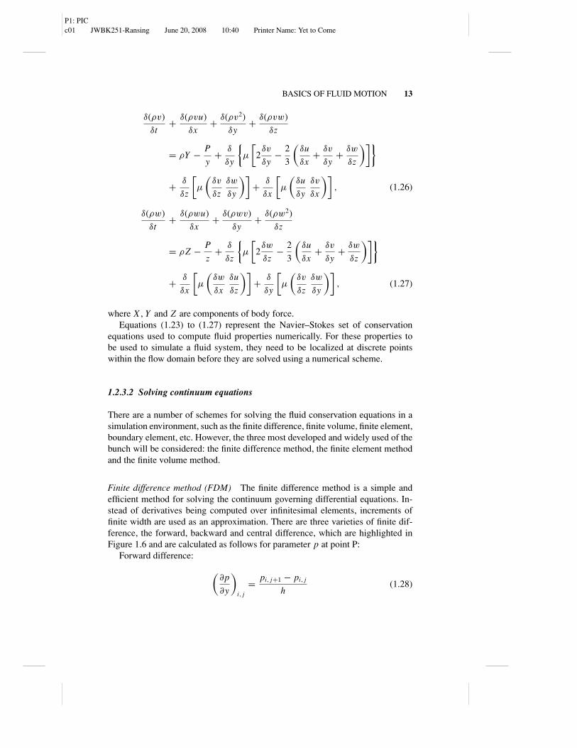
Finite difference method (FDM) The finite difference method is a simple andefficient method for solving the continuum governing differential equations. In-stead of derivatives being computed over infinitesimal elements, increments offinite width are used as an approximation. There are three varieties of finite dif-ference, the forward, backward and central difference, which are highlighted inFigure 1.6 and are calculated as follows for parameter p at point P:

Forward difference:

(∂p

∂y

)i, j

= pi, j+1 − pi, j

h(1.28)



y

h

h

x

P

i, j +1

i,j −1

i,j i−1,j i +1,j

Figure 1.6 Illustrating the finite difference method calculations at point P.

Backward difference: (∂p

∂y

)i, j

= pi, j − pi, j−1

h(1.29)

Central difference: (∂p

∂y

)i, j

= pi, j+1 − pi, j−1

2h(1.30)

Using this method the partial differential equations can be replaced with simplealgebraic equations that can be solved either iteratively or by matrix inversion.This can be implemented for fluid flow simulations to yield the values of the flowvariables at discrete points in the flow field. Due to the structures of the FDM,problems are limited to ones with simple boundaries where a structured mesh canbe used. For more complex problems, the finite element method allows for moreversatility but is much more complex.

Finite element method (FEM) The aim of the finite element method is to de-termine the values of the dependent variables of the conservative flow equations.The FEM achieves this by dividing the flow domain into a finite number of cellsor elements, each containing a small portion of the continuous fluid. At pointsplaced at the corners or sides of these elements, points that are known as nodes,the governing equations are evaluated (see Figure 1.7). Instead of working withthe differential equations directly, the FEM uses these nodes to discretize andevaluate the governing equations in an integral form using weighting functions.



Figure 1.7 Governing equations evaluated at nodes surrounding fluid elements.

Finite volume method (FVM) Similar to the finite element method, the FVMdiscretizes the flow domain into elemental control volumes surrounding a node.Flow parameters are then treated as fluxes between control volumes, and conser-vation is maintained in each element. This allows for better treatment of flowswith discontinuities such as shock waves.

1.2.3.3 Advantages

Continuum simulations are able to provide an accurate model for fluid behaviourin a wide range of applications and systems. The division of the flow field into dis-crete elements allows complex geometries to be simulated, and smaller elementscan be used to refine the solution in areas of high gradients or where a greateraccuracy is needed.

By approximating the fluid as a continuum and ignoring the underlying molec-ular behaviour, a great deal of computational effort is saved and accuracy has beenproved to be sufficient in many applications. The molecular information can beapproximated at these scales, as the molecular motion cancels out, yielding onlybulk properties at this scale.

Continuum simulations also have the flexibility to prescribe a wide variety ofboundary conditions capable of replicating almost any system, while still main-taining global conservation laws.

1.2.3.4 Limitations

Continuum mechanics, however, has its drawbacks. It is dependent on the gener-ation of the mesh of elements and nodes it uses in the approximation. The gen-eration of these meshes can be almost as time consuming and challenging as theactual simulation. These meshes can also have a significant effect on the solution,



either through resolution or the distribution of nodes, and must be generated withconsideration for the system of interest.

The scale of the system is also limited by the continuum approximations. Be-cause of the continuum approximations, the matter of interest must be uniformthroughout and infinitely divisible. This removes the ability to deal with discreteobjects, such as, at the top of the scale, extreme planetary systems and, at thelower end, molecules. As the continuum governing equations are approximate re-lationships which are approximated in their solution, careful validation and testingmust also be performed, which is true of any simulation method. Particular caremust also be taken close to the continuum limit.

The breakdown of these approximations in the meso scale region between thecontinuum and molecular scales was studied in detail and the transition from con-tinuum to molecular scale effects is explained in depth in later sections.

1.3 MOLECULAR MECHANICS

At very small scales (≤ 10−8), the mechanics of fluid take on an entirely dif-ferent form. The continuum approximations and laws are not valid as the num-ber of molecules in the system is of the order of tens to thousands. At thisscale the molecular interactions dominate the physics of the fluid, and it is de-batable whether fluid is an accurate description as it is better described as amolecular flow.

1.3.1 Molecular Properties

The properties at a molecular scale (∼ 10−9) are very different from those con-sidered at the bulk/continuum scale. At this scale, the characteristic length of theflow is comparable to the diameters of individual molecules. There is no conceptof bulk properties, and fluid-like motion is in the form of the motion of individualmolecules. The fluid is now not continuous, as the molecular centres representdiscontinuities in both density and energy.

The molecular chemistry of the making or breaking of bonds or changes tothe internal structure of molecules is not considered in this research, althoughit is important to understand the mechanisms by which molecules interact in achemically stable fluid.

A molecule is formed of an aggregate of two or more atoms bonded togetherby special bonding forces. The examination of interactions between bondedmolecules was first undertaken by a Dutch chemist, Johannes Diderik van derWaals, whose studies into noble gases led to the characterization of the forcesbetween molecules [8]. The van der Waals force was originally considered to


MOLECULAR MECHANICS 17

0.0045

0.0035

0.0025

−0.0025

0.0015

−0.0015

0.0005

−0.0005

Po

ten

tial

en

erg

y

Radius from molecule centre

0 1 2 3 4 5 6 7 8 9 10

Van der WaalsRepulsive, Pauli, forcesAttractive, London, forces

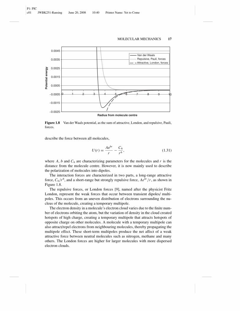
Figure 1.8 Van der Waals potential, as the sum of attractive, London, and repulsive, Pauli,forces.

describe the force between all molecules,

U (r ) = Aebr

r− C6

r6, (1.31)

where A, b and C6 are characterizing parameters for the molecules and r is thedistance from the molecule centre. However, it is now mainly used to describethe polarization of molecules into dipoles.

The interaction forces are characterized in two parts, a long-range attractiveforce, C6/r6, and a short-range but strongly repulsive force, Aebr/r , as shown inFigure 1.8.

The repulsive forces, or London forces [9], named after the physicist FritzLondon, represent the weak forces that occur between transient dipoles/ multi-poles. This occurs from an uneven distribution of electrons surrounding the nu-cleus of the molecule, creating a temporary multipole.

The electron density in a molecule’s electron cloud varies due to the finite num-ber of electrons orbiting the atom, but the variation of density in the cloud createdhotspots of high charge, creating a temporary multipole that attracts hotspots ofopposite charge on other molecules. A molecule with a temporary multipole canalso attract/repel electrons from neighbouring molecules, thereby propagating themultipole effect. These short-term multipoles produce the net affect of a weakattractive force between neutral molecules such as nitrogen, methane and manyothers. The London forces are higher for larger molecules with more dispersedelectron clouds.



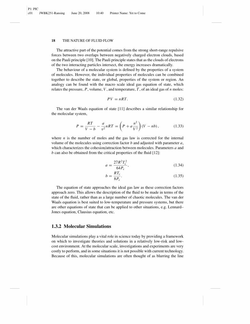
The attractive part of the potential comes from the strong short-range repulsiveforces between two overlaps between negatively charged electron clouds, basedon the Pauli principle [10]. The Pauli principle states that as the clouds of electronsof the two interacting particles intersect, the energy increases dramatically.

The behaviour of a molecular system is defined by the properties of a systemof molecules. However, the individual properties of molecules can be combinedtogether to describe the state, or global, properties of the system or region. Ananalogy can be found with the macro scale ideal gas equation of state, whichrelates the pressure, P , volume, V , and temperature, T , of an ideal gas of n moles:

PV = n RT . (1.32)

The van der Waals equation of state [11] describes a similar relationship forthe molecular system,

P = RT

V − b− a

v2n RT =

(P + a

n2

V 2

)(V − nb) , (1.33)

where n is the number of moles and the gas law is corrected for the internalvolume of the molecules using correction factor b and adjusted with parameter a,which characterizes the cohesion/attraction between molecules. Parameters a andb can also be obtained from the critical properties of the fluid [12]:

a = 27R2T 2c

64Pc, (1.34)

b = RTc

8Pc. (1.35)

The equation of state approaches the ideal gas law as these correction factorsapproach zero. This allows the description of the fluid to be made in terms of thestate of the fluid, rather than as a large number of chaotic molecules. The van derWaals equation is best suited to low-temperature and pressure systems, but thereare other equations of state that can be applied to other situations, e.g. Lennard–Jones equation, Clausius equation, etc.

1.3.2 Molecular Simulations

Molecular simulations play a vital role in science today by providing a frameworkon which to investigate theories and solutions in a relatively low-risk and low-cost environment. At the molecular scale, investigations and experiments are verycostly to perform, and in some situations it is not possible with current technology.Because of this, molecular simulations are often thought of as blurring the line


MOLECULAR MECHANICS 19

between experiment and simulation, as they can be used to investigate theoriesthat otherwise could not be tested.

Molecular simulation is the study of material/fluid by considering the individ-ual interactions of atoms or molecules, and will be described in detail in Chapter 2.General simulation schemes involve representative molecules interacting withsome sort of boundary and each other to achieve a change in position and mo-mentum. There are many different forms of simulation methods and techniquesthat can be applied to many different situations, each offering different advan-tages. The basic mechanism behind almost all molecular simulations is relativelybasic, relying on a system of particles that represent atoms or molecules that in-teract using Newton’s law,

F = ma, (1.36)

where the force acting on a particle, F , is equal to its mass, m, multiplied by itsacceleration, a. The force acting on any one of the many particles in the system isdetermined by the movement of those around it. There are two branches of molec-ular simulation, stochastic and deterministic. The deterministic approach is in theform of a molecular dynamic (MD) simulation, where the outcome could theo-retically be worked out. Stochastic methods, such as the Monte Carlo simulationmethod, have an element of unpredictability and chance and the result cannot beexactly calculated in advance; these will be discussed in more detail later. Despitethe deterministic approach of standard molecular dynamics, it remains a statisti-cal mechanics method, as system property values are developed from ensembleaverages over the system.

Molecular simulations rely on representative molecules interacting with eachother, so each molecule must possess individual properties that determine how itwill move in the next time step; these are position, r , and momentum, p, applied inthe number of dimensions present in the simulation. It is from these properties thatinteractions and collisions are found and evaluated, thus allowing the simulationto proceed. Given that the state of the whole system is governed by a function ofthe properties of all the individual particles, the concept of ‘phase space’ can beintroduced. At any time in the simulation, the state of the system can be definedby a single point in a 6N -dimensional ‘phase space’, where N is the number ofparticles in a three-dimensional system. Each three-dimensional particle containsinformation about its momentum (px , py , pz) and position (x , y, z) in each ofthe three dimensions, so for N particles there are 6N variables. As the simulationprogresses, the phase point will move throughout phase space, sampling moreof the regions accessible without violating any of the rules set at the start of thesimulation, such as constant energy, pressure or temperature.

In the following sections the basics behind simulations of molecular systemswill be described, before proceeding to a description of how it applies to real fluidflow problems and situations.



1.4 TYPES OF SIMULATION

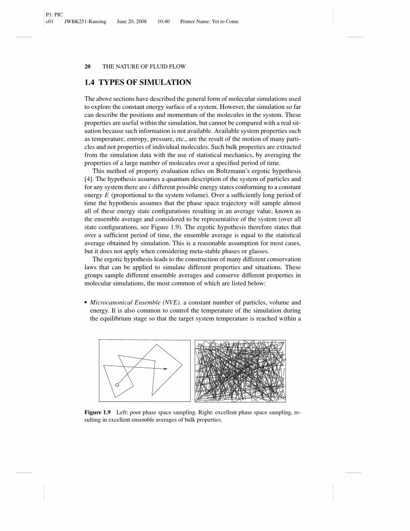
The above sections have described the general form of molecular simulations usedto explore the constant energy surface of a system. However, the simulation so farcan describe the positions and momentum of the molecules in the system. Theseproperties are useful within the simulation, but cannot be compared with a real sit-uation because such information is not available. Available system properties suchas temperature, entropy, pressure, etc., are the result of the motion of many parti-cles and not properties of individual molecules. Such bulk properties are extractedfrom the simulation data with the use of statistical mechanics, by averaging theproperties of a large number of molecules over a specified period of time.

This method of property evaluation relies on Boltzmann’s ergotic hypothesis[4]. The hypothesis assumes a quantum description of the system of particles andfor any system there are i different possible energy states conforming to a constantenergy E (proportional to the system volume). Over a sufficiently long period oftime the hypothesis assumes that the phase space trajectory will sample almostall of these energy state configurations resulting in an average value, known asthe ensemble average and considered to be representative of the system (over allstate configurations, see Figure 1.9). The ergotic hypothesis therefore states thatover a sufficient period of time, the ensemble average is equal to the statisticalaverage obtained by simulation. This is a reasonable assumption for most cases,but it does not apply when considering meta-stable phases or glasses.

The ergotic hypothesis leads to the construction of many different conservationlaws that can be applied to simulate different properties and situations. Thesegroups sample different ensemble averages and conserve different properties inmolecular simulations, the most common of which are listed below:

� Microcanonical Ensemble (NVE). a constant number of particles, volume andenergy. It is also common to control the temperature of the simulation duringthe equilibrium stage so that the target system temperature is reached within a

Figure 1.9 Left: poor phase space sampling. Right: excellent phase space sampling, re-sulting in excellent ensemble averages of bulk properties.


TYPES OF SIMULATION 21

suitable number of time steps. The simplest form of temperature control is toscale the velocities periodically, but this is not a truly isothermal method andmust be removed before the properties are collected.

Although energy is considered to be conserved, there will be slight fluctua-tions and the possibility of a small drift due to truncation and rounding errorsfrom the calculations.

This type of ensemble is useful for predicting thermodynamic responsefunctions.

� Canonical Ensemble (NVT). a constant number of particles, volume and tem-perature. As in the microcanonical ensemble, during the initialization stage thevelocities are scaled to the desired value for the set temperature. Although use-ful for initialization, velocity scaling is not suitable to use as a control for asimulation as it is crude and not a truly isothermal method. Therefore, otherthermostatic methods must be used to apply the temperature control, which willbe explained in detail in Chapter 3. This ensemble is used to perform confor-mational (spatial arrangements of a molecule) searches of models evaluated ina vacuum without periodic boundary conditions. Even when periodic boundaryconditions are used, this ensemble can be useful if pressure is not a significantfactor, as the constant temperature and volume provides less perturbation dueto the absence of pressure coupling.

� Isobaric–Isothermal Ensemble (NPT and NST).

– NPT: a constant number of particles, pressure and temperature. Tempera-ture is controlled using one of the thermostatic schemes detailed in Chap-ter 3 and the pressure is controlled by varying the volume of the system us-ing the Berendsen, Anderson or the Parrinello–Rahman schemes [13]. TheBerendsen and Anderson schemes work by varying the size of the system,while the Parrinello-Rahman scheme is also capable of varying the shape ofthe system.

– NST: a constant number of particles, stress and temperature. This is an ex-tension to the constant pressure ensemble, which adds extra control on thestress components xx , yy, zz, xy, yz and zx .

Both methods are mainly used in structural applications. NST can be used toevaluate stress/strain relationships and NPT is generally used when the correctpressure, volume and temperature are important.

� NPH and NSH.

– NPH: a constant number of particles, pressure and enthalpy. This ensem-ble is similar to the NVT ensemble, only the size on the cell is allowedto vary.



R

l

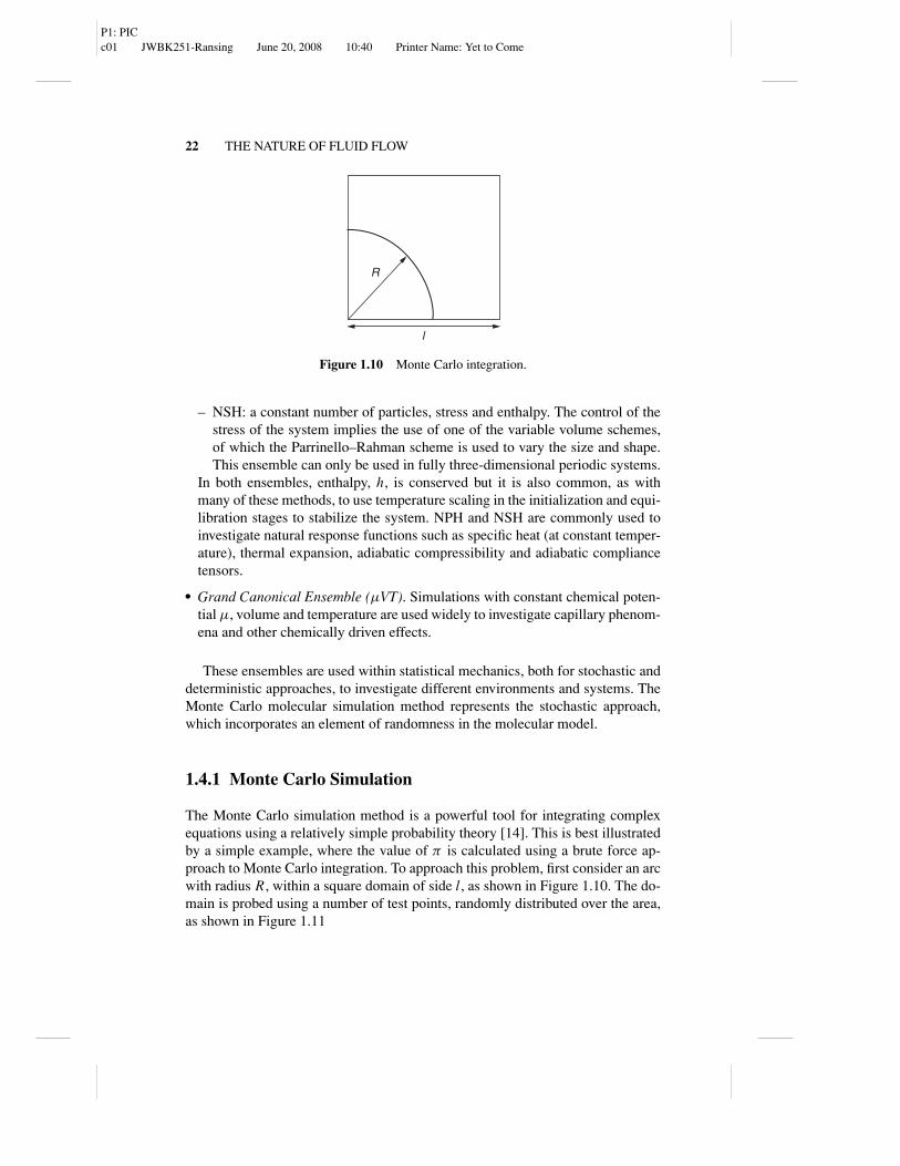
Figure 1.10 Monte Carlo integration.

– NSH: a constant number of particles, stress and enthalpy. The control of thestress of the system implies the use of one of the variable volume schemes,of which the Parrinello–Rahman scheme is used to vary the size and shape.This ensemble can only be used in fully three-dimensional periodic systems.

In both ensembles, enthalpy, h, is conserved but it is also common, as withmany of these methods, to use temperature scaling in the initialization and equi-libration stages to stabilize the system. NPH and NSH are commonly used toinvestigate natural response functions such as specific heat (at constant temper-ature), thermal expansion, adiabatic compressibility and adiabatic compliancetensors.

� Grand Canonical Ensemble (µVT). Simulations with constant chemical poten-tial µ, volume and temperature are used widely to investigate capillary phenom-ena and other chemically driven effects.

These ensembles are used within statistical mechanics, both for stochastic anddeterministic approaches, to investigate different environments and systems. TheMonte Carlo molecular simulation method represents the stochastic approach,which incorporates an element of randomness in the molecular model.

1.4.1 Monte Carlo Simulation

The Monte Carlo simulation method is a powerful tool for integrating complexequations using a relatively simple probability theory [14]. This is best illustratedby a simple example, where the value of π is calculated using a brute force ap-proach to Monte Carlo integration. To approach this problem, first consider an arcwith radius R, within a square domain of side l, as shown in Figure 1.10. The do-main is probed using a number of test points, randomly distributed over the area,as shown in Figure 1.11



Figure 1.11 Monte Carlo integration; domain is interrogated by random points, some ofwhich lie within the arc.

The area inside the arc is then estimated by the ratio of the number of pointsinside its constraints (squares) and the total number of points (squares + circles):

Squares

Circles + squares= area of arc

area of square, (1.37)

which becomes

Area of arc = Number of squares

Number of circles + number of squares× area of square.

(1.38)The equation for the area of an arc is known as π R2, so this becomes

π R2

4= squares

circles + squares× l2. (1.39)

Rearranging for π gives

π = squares

circles + squares

4l2

R2. (1.40)

Equation (1.40) relates the ratio of particles within the arc to the value of π .The accuracy of the estimation is mainly dependent on the number of points usedto probe the domain. This approach is known as the brute force approach, and isthe less sophisticated form of Monte Carlo integration, where there is an equalprobability for a sample point to be taken from anywhere within the domain.

Monte Carlo simulation uses elements from this technique to move themolecules in the system in the following way:

1. A molecule is selected at random from the system.

2. The molecule is then moved a random distance in a random direction.



3. The resulting change in potential energy of the whole system is then evaluatedand if it is reduced, the move is accepted.

4. Some failed moves are also accepted according to a probability value, P . Com-pletely rejected moves are ignored.

The distance a particle is moved is often scaled to alter the acceptance ratio ofmoves making the simulation more efficient.

When applied to molecular simulation there is a need to improve computa-tional efficiency by making certain approximations for solving equations on rela-tively inactive regions. It is at this point that importance sampling techniques areintroduced into the Monte Carlo method, as described by Metropolis et al. [15].

The Metropolis Monte Carlo method biases the contribution of each move tothe statistical average based on the Boltzmann factor. The probability of a particlebeing selected is also influenced by the Boltzmann factor as follows:

1. The overall system energy is calculated, Ei .

2. From the system, one molecule is picked out. The probability of selection foreach particle is determined by the probability parameter A.

3. The molecule is assigned a small perturbation, such as a small displacement inposition, and the new system energy is calculated, E j .

4. If the new system energy is smaller than the old system energy, accept theaddition of the perturbation.

5. If the new system energy is greater than the old system energy, accept the per-turbation with probability B = e−E j −Ei /kbT (note that β = e−E/kbT is the Boltz-mann factor).

6. Repeat steps 1 to 5.

This gives the probability value that an added perturbation will be accepted asA multiplied by B. Allowing a small proportion of moves that increase the systemenergy to be accepted provides a limited amount of protection against settling inmeta-stable configurations on quasi-equilibrium states. By doing this, the systemis pushed towards the configuration that is most likely to occur, thus speeding upthe simulation run time.

Another modified form of the Monte Carlo technique is the force biasedmethod [16]. This adds some extra calculation overheads into each molecule eval-uation to determine the resultant force acting on the particle by its neighbours,biasing the random move performed within the simulation. This also improvesthe computational efficiency as statistical averages need to sample fewer configu-rations.



Additional information on the Monte Carlo simulation method and its differentensembles can be found in the book by Gould et al. [17]. Gould provides examplesof Monte Carlo methods, focusing on its advantages at simulating phase changes,which has been used to good effect by Levesque et al. [18] applied to hydrogenstorage in carbon nanotubes.

1.4.2 Molecular Dynamics

Molecular dynamic (MD) simulations model fluid in two ways, with moleculesbeing represented as hard or soft spheres. Modelling with hard sphere modelsprovides a relatively simple approach to approximating a system of molecules butstill has valid applications, such as looking into the liquid–gas phase transitionand diffusion, and hard sphere fluids have a well-defined critical point. The draw-backs are mainly to do with the discontinuous nature of the model. The collisionsare performed instantaneously and spheres only interact repulsively, whereas realsystems have some form of attraction between particles. Because of this, it is alsoused for gas simulations where the distances between molecules are far greaterthan their diameter, and intermolecular interactions occur rarely. Despite thesedisadvantages, the model is still widely and successfully used, but care must betaken to ensure that it is appropriate to the situation being simulated.

A more realistic, but more complex and computationally demanding approach,is the soft sphere model. In this model, the long-range attractive and repulsiveforces are modelled as a continuous function of the separation between pairs ofmolecules. The use of a continuous interaction function improves the accuracy ofthe simulation at the cost of increasing the computational load.

1.4.3 Introduction to the Physics of MD Simulations

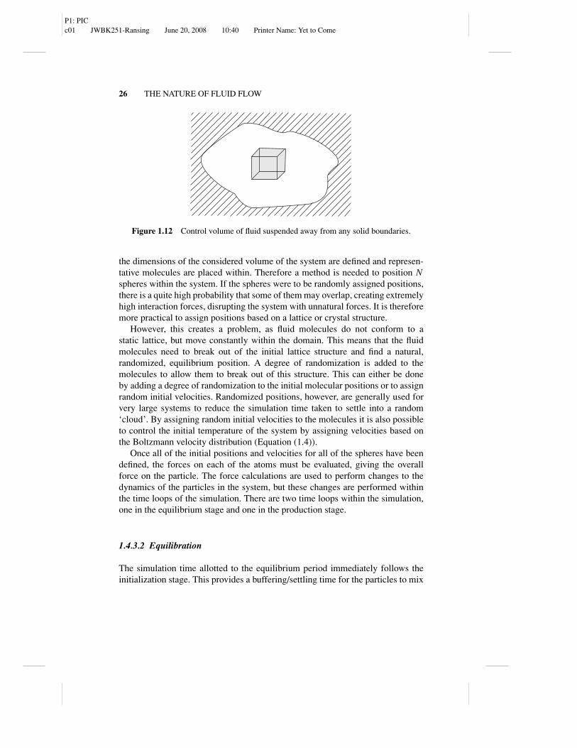
Molecular dynamic simulations work on the same basic principles regardless ofthe actual interaction laws (hard or soft spheres) and rely on the following threesteps: initialization, equilibrium and production. These stages are detailed belowfollowing the example of a molecular scale cubic cell suspended in a fluid awayfrom any physical boundaries, as shown in Figure 1.12.

1.4.3.1 Initialization

When the simulation is run, the first task performed is to define the problem; thisis known as initialization. This stage of the simulation accounts for only one timestep and is used to create the system of spheres based on a set of user-definedparameters. In the example used, a control volume suspended in a fluid of setvolume and density is simulated (Figure 1.12). The initialization stage is where



Figure 1.12 Control volume of fluid suspended away from any solid boundaries.

the dimensions of the considered volume of the system are defined and represen-tative molecules are placed within. Therefore a method is needed to position Nspheres within the system. If the spheres were to be randomly assigned positions,there is a quite high probability that some of them may overlap, creating extremelyhigh interaction forces, disrupting the system with unnatural forces. It is thereforemore practical to assign positions based on a lattice or crystal structure.

However, this creates a problem, as fluid molecules do not conform to astatic lattice, but move constantly within the domain. This means that the fluidmolecules need to break out of the initial lattice structure and find a natural,randomized, equilibrium position. A degree of randomization is added to themolecules to allow them to break out of this structure. This can either be doneby adding a degree of randomization to the initial molecular positions or to assignrandom initial velocities. Randomized positions, however, are generally used forvery large systems to reduce the simulation time taken to settle into a random‘cloud’. By assigning random initial velocities to the molecules it is also possibleto control the initial temperature of the system by assigning velocities based onthe Boltzmann velocity distribution (Equation (1.4)).

Once all of the initial positions and velocities for all of the spheres have beendefined, the forces on each of the atoms must be evaluated, giving the overallforce on the particle. The force calculations are used to perform changes to thedynamics of the particles in the system, but these changes are performed withinthe time loops of the simulation. There are two time loops within the simulation,one in the equilibrium stage and one in the production stage.

1.4.3.2 Equilibration

The simulation time allotted to the equilibrium period immediately follows theinitialization stage. This provides a buffering/settling time for the particles to mix



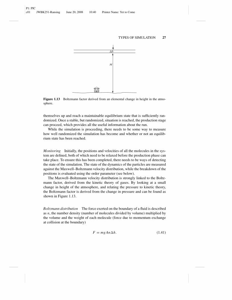
H

∆h

Figure 1.13 Boltzmann factor derived from an elemental change in height in the atmo-sphere.

themselves up and reach a maintainable equilibrium state that is sufficiently ran-domized. Once a stable, but randomized, situation is reached, the production stagecan proceed, which provides all the useful information about the run.

While the simulation is proceeding, there needs to be some way to measurehow well randomized the simulation has become and whether or not an equilib-rium state has been reached.

Monitoring Initially, the positions and velocities of all the molecules in the sys-tem are defined, both of which need to be relaxed before the production phase cantake place. To ensure this has been completed, there needs to be ways of detectingthe state of the simulation. The state of the dynamics of the particles are measuredagainst the Maxwell–Boltzmann velocity distribution, while the breakdown of thepositions is evaluated using the order parameter (see below).

The Maxwell–Boltzmann velocity distribution is strongly linked to the Boltz-mann factor, derived from the kinetic theory of gases. By looking at a smallchange in height of the atmosphere, and relating the pressure to kinetic theory,the Boltzmann factor is derived from the change in pressure and can be found asshown in Figure 1.13.

Boltzmann distribution The force exerted on the boundary of a fluid is describedas n, the number density (number of molecules divided by volume) multiplied bythe volume and the weight of each molecule (force due to momentum exchangeat collision at the boundary)

F = mg An�h. (1.41)



Therefore pressure becomes

�P = − F

A= −mg An�h

A, (1.42)

�P = −mgn�h. (1.43)

The ideal gas law can be rearranged for n:

Pv = NkbT, n = N

V= P

kbT, (1.44)

which when substituted into the expression for �P gives

�P = −mg�h

kbTP. (1.45)

Thus, for h → 0, ∫1

PdP = − mg

kbT

∫dh (1.46)

gives

P = P0e−mgh/kbT , (1.47)

where e−mgh/kbT is known as the Boltzmann factor. This form of the Boltzmannfactor has been derived from potential energy, and as potential energy, can bewritten as mgh, the factor can be rewritten as

β = e−EPE/kbT , (1.48)

where E is the energy. A similar derivation can be performed using kinetic energy,resulting in a Boltzmann factor of

β = e−EKE/kbT . (1.49)

This describes the probability that a molecule is at a certain energy level for aprescribed temperature, T . By normalizing probability values so they add to a unitvalue, the Boltzmann factor can be evaluated over a range of speeds to obtain the

Maxwell–Boltzmann distribution for speeds. Where speed v =√

v2x + v2

y + v2z ,

f (v) = 4π( m

2π RT

)2/3v2e−mv2/(2RT ). (1.50)



0.0016

0.0014

0.0012

0.001

0.0008

0.0006

0.0004

0.0002

00 200 400 600 800 1000 1200 1400 1600 1800 2000

1000 K

500 K

400 K

300 K

Pro

bab

ility

Molecule Speed (m/s)

Figure 1.14 Maxwell distribution of velocity for temperatures of 300 K, 400 K, 500 Kand 1000 K.

This velocity–probability distribution (Figure 1.14) can therefore be used toassess the dynamics of a simulation, by comparing the distribution of the resul-tant velocity of molecules with this distribution. This is an important test, as evenfor systems at steady state, as the velocity of individual particles does not remainconstant, they are constantly interacting and colliding with each other. It is sen-sible to consider the overall distribution of velocities within the system to get aview of how the system is behaving and how it is approaching equilibrium.

By monitoring the distribution of velocities and its resemblance to theMaxwell–Boltzmann distribution, a measure of the approach to equilibrium isdeveloped. It is then used to identify stability in the simulation. If the simulationis not stable, the temperature would fluctuate and the system would not be in equi-librium. It is therefore necessary to observe the development of the distributionover a period of time, ensuring that it converges with minimal oscillations. Thegraphs in Figure 1.14 show examples of the distribution at different temperatures.

The variations arise from statistical noise that occurs due to the finite numberof molecules in the simulation. The greater the number of molecules, the loweris the noise in the extracted distribution. For an infinite number of molecules,the distribution would be followed perfectly, going the possibility of a continuumdescription.

Other measured thermodynamic properties, such as pressure and density, arealso sensitive to the state of the system. By looking at these properties and seeinghow they behave is another tool in the identification of equilibrium and smoothrunning of the simulation. Properties are averaged over a period of time and need



time to adjust themselves to the correct, stable value. If some instabilities arepresent and the properties are not converging, the system cannot be in a steadystate.

The stability of a property does not just imply that the value remains approxi-mately constant, but it should also be able to recover its value after a small amountof perturbation, such as a temperature adjustment.

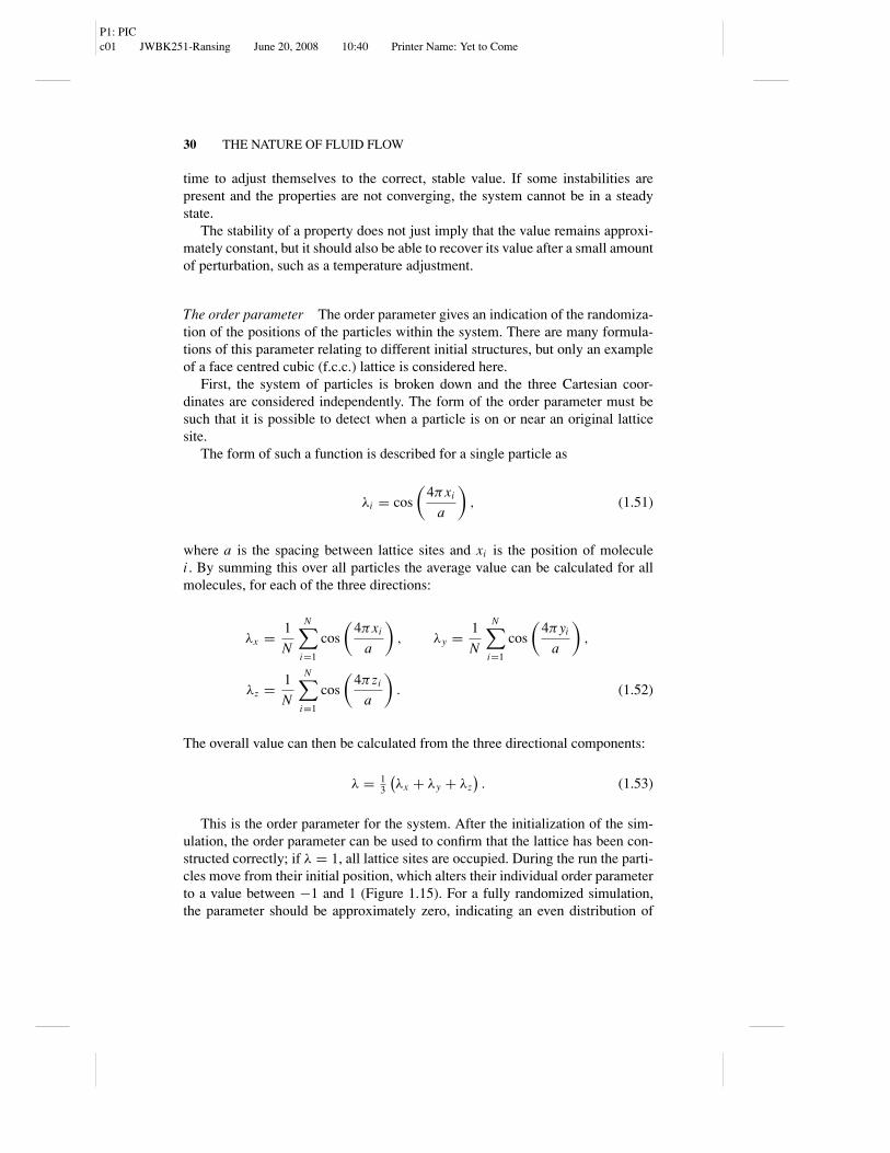
The order parameter The order parameter gives an indication of the randomiza-tion of the positions of the particles within the system. There are many formula-tions of this parameter relating to different initial structures, but only an exampleof a face centred cubic (f.c.c.) lattice is considered here.

First, the system of particles is broken down and the three Cartesian coor-dinates are considered independently. The form of the order parameter must besuch that it is possible to detect when a particle is on or near an original latticesite.

The form of such a function is described for a single particle as

λi = cos

(4πxi

a

), (1.51)

where a is the spacing between lattice sites and xi is the position of moleculei . By summing this over all particles the average value can be calculated for allmolecules, for each of the three directions:

λx = 1

N

N∑i=1

cos

(4πxi

a

), λy = 1

N

N∑i=1

cos

(4πyi

a

),

λz = 1

N

N∑i=1

cos

(4π zi

a

). (1.52)

The overall value can then be calculated from the three directional components:

λ = 13

(λx + λy + λz

). (1.53)

This is the order parameter for the system. After the initialization of the sim-ulation, the order parameter can be used to confirm that the lattice has been con-structed correctly; if λ = 1, all lattice sites are occupied. During the run the parti-cles move from their initial position, which alters their individual order parameterto a value between −1 and 1 (Figure 1.15). For a fully randomized simulation,the parameter should be approximately zero, indicating an even distribution of



1

−1

λia Lattice positions in one dimension

Figure 1.15 Order parameter relative to lattice positions.

particles between the bounds of the simulation. The order parameter can also beused to determine the point of solidification and the quality of the lattice, as usedby Radhakrishnan and Gubbins [19].

A successfully equilibrated system should be sufficiently randomized and havereached a stable equilibrium point from which the production phase can begin.The stable point should have the same global properties regardless of the initialpositions of the molecules, and can be tested by applying random noise to thepositions of the molecular lattice and examining several equilibration phases. Afully equilibrated system will have the following properties:

� Stable levels of kinetic, potential and total energy. Variations in energy levelsare to be expected, but there should be no drift in average values of energy.

� The order parameter should be zero, indicating that the molecules are suffi-ciently randomized.

� Velocities of all molecules should conform to velocity distributions for the settemperature for the system.

� Stable state which is independent of initial positions of molecules.

Although the above criteria help identify equilibrium, there is still a chance forundetected instabilities to be present, so care must be taken to be certain thata steady state has been reached. After sufficient randomization, the productionphase of the simulation can begin.

1.4.3.3 Production

After the successful randomization of the system of molecules, the productionphase can take place. This is basically an extension of the equilibrium phase tocalculate the properties of the stable system over a set period of time. As the sys-tem is assumed to be sufficiently equilibrated, some of the controlling factors andadjustments are removed to allow the simulation to progress freely. Although the



controls are removed, the parameters such as the order parameter and velocitydistribution are still monitored to check for anomalies. At the end of the equili-bration phase, all property averages are reset to zero so that when the productionphase starts, the properties are not affected by the approach to equilibrium and arethe result of the production phase only.

This is the stage of the simulation where the interrogation and investigation ofthe system may start. There are two main types of dynamic models used in simu-lation to describe molecular dynamics, hard sphere and soft sphere. They differ inthe way they handle interactions between particles. The hard sphere model consid-ers interactions as binary collisions, whereas the soft sphere approach considersthe molecules to be continually interacting via long-range potential functions withtheir neighbours.

1.4.4 Hard sphere model

Hard sphere simulations only interact by colliding with one another and exchang-ing linear momentum in a perfectly elastic way. The forces present in the hardsphere model are relatively simple and easy to calculate. As there are no long-range interactions, spheres only interact when they are colliding. The hard spheremodels are generally event driven, where the simulation time only steps forwardto the next event, or collision. This is based on the assumption that all sphereshave an initial position and velocity, and that sphere travels along the same direc-tion at a constant speed (as there is no acceleration), such that the position at anytime can be calculated as follows [4]:

ri (t) = ri (t0) + (t − t0)vi (t0) (1.54)

where ri and vi are the position (of the centre of the sphere) and velocity of particlei , t0 is the start time and t is the new time. As all molecules move in this way thetime until two spheres overlap, i.e. when a collision occurs, can be predicted,highlighting the deterministic nature of the molecular dynamics approach.

At any collision between two spheres, each with diameter σ , the distance be-tween the centres will be σ . Therefore a collision occurs between two moleculeswith position at time t , of r1(t) and r2(t), when

|r1(t) − r2(t)| = σ, (1.55)

which can be calculated as

[r1(t) − r2(t)]2 = σ 2. (1.56)



At this time, t , a collision is occurring and in a simulation of N molecules themolecules that are colliding next need to be determined. By substituting Equa-tion 1.54 for r1 and r2 in Equation (1.56) and rearranging for t , the time at whichthe two spheres will collide is given as

tc = t0 +(−v12r12) ±

√(v12r12)2 − v12(r2

12 − σ 2)

v212

, (1.57)

where

v12 = (tc − t0)v1 − (tc − t0)v2, (1.58)

r12 = r1(t) − r2(t). (1.59)

This gives the collision time, tc, for two spheres providing they are moving to-wards each other. Therefore, before tc is calculated, the state of the collision forthe colliding pair must be determined.

For example, take molecule 1 from the simulation and consider the possibilitythat it may collide with molecule 37. There are two basic possibilities, either theyare moving towards each other or away. Mathematically, this is described by theprojection of the velocity difference along the line of the centres of the spheresby finding the product of v12 and r12. If the result is less than zero, the spheres aremoving together:

v12r12 < 0. (1.60)

If the spheres satisfy this condition, they are said to be moving towards each other,but this does not guarantee a collision. To determine if they will collide we needto consider the limiting case where they come in contact as they pass each other.

By considering the one sphere to be fixed and the other to have velocity equalto the velocity difference, Figure 1.16 shows the limiting case for collision. Itcan be seen that, there must be a limiting value of θ that, if exceeded, ensure nocollisions occur and the spheres pass each other [4].

r12

v12

θσ

Figure 1.16 Hard sphere collision detection.



This collision test is evaluated for every possible colliding pair within the sys-tem by looping over all molecules and calculating the next collision time for each.From these times, a table of collision times is created containing predictions forwhen each sphere will have its next collision. The calculation of this table is thelast step in the initialization stage.

The table can then be used and updated in the equilibrium and productionstages to advance the simulation and evaluate the next collision.

Collisions are modelled as binary interactions, occurring instantaneously,where the molecules exchange linear momentum.

1.4.4.1 Time steps

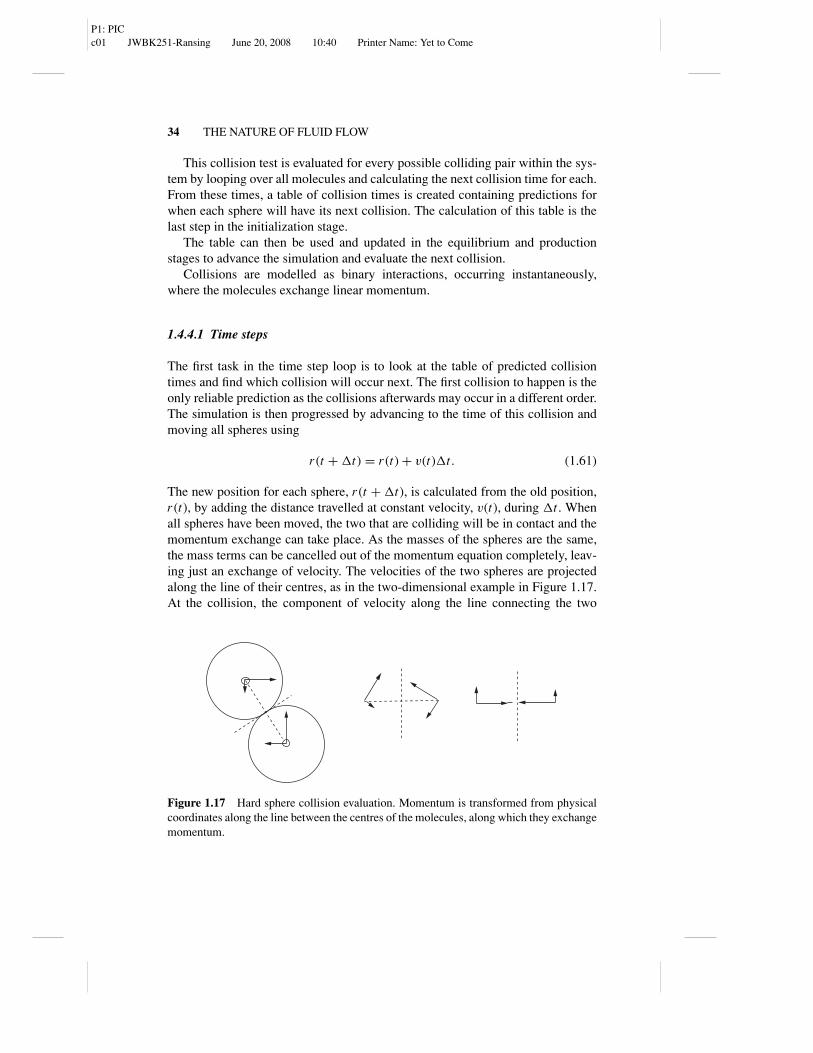
The first task in the time step loop is to look at the table of predicted collisiontimes and find which collision will occur next. The first collision to happen is theonly reliable prediction as the collisions afterwards may occur in a different order.The simulation is then progressed by advancing to the time of this collision andmoving all spheres using

r (t + �t) = r (t) + v(t)�t. (1.61)

The new position for each sphere, r (t + �t), is calculated from the old position,r (t), by adding the distance travelled at constant velocity, v(t), during �t . Whenall spheres have been moved, the two that are colliding will be in contact and themomentum exchange can take place. As the masses of the spheres are the same,the mass terms can be cancelled out of the momentum equation completely, leav-ing just an exchange of velocity. The velocities of the two spheres are projectedalong the line of their centres, as in the two-dimensional example in Figure 1.17.At the collision, the component of velocity along the line connecting the two

Figure 1.17 Hard sphere collision evaluation. Momentum is transformed from physicalcoordinates along the line between the centres of the molecules, along which they exchangemomentum.



centres is exchanged, while the component of velocity perpendicular to this lineremains the same for both spheres. The velocities of both spheres are updated andcan be used to update the prediction table for the next collision time for the pair.There is no need to update the table for all the molecules, as only the colliding pairexperience a change in velocity. The updated tables can then be used to predictthe time step to the next collision.

1.4.5 Soft sphere model

The soft sphere model of molecular interactions considers molecules to interactby exerting a force on each other relative to the distance between them. Theseinteractions occur continually, with each molecule having a ‘zone’ in which anyother molecule present is influenced. Hard spheres will only interact when contactis made.

The initialization stage starts as stated above, where the initial positions andvelocities have been defined for all molecules in the system. Force calculation forsoft sphere models is more complex due to the addition of long-range interactions.Particles in the system continually attract and repel their neighbours through apredefined potential function, as opposed to the instantaneous and perfectly elasticcollisions of the binary collisions described above.

This is best described with the use of Figure 1.18, where the centre particleis interacting with particles within a set radius, RC. The most common potentialused is the Lennard–Jones 12-6 potential, which provides an approximation of theattractive and repulsive forces experienced by nonbonded molecules.

RN

RC

Figure 1.18 Soft sphere interaction detection.



The potential functions are continuous and become weaker as the distancebetween molecules increases, so it is therefore convenient to set a limit to the‘zone of influence’ (typically around 2 to 3 times the interaction radius of themolecules) of any one molecule (outside which the potential is approximatelyzero). This finite limit cuts off the weak, long-range interactions between far-offparticles, interactions that can be approximated by ‘long-range correction fac-tors’ [4] to increase the efficiency of the simulation. Despite this streamlining,the process of finding a particle neighbour is time consuming and there needsto be an effective method of storing the lists of neighbouring particles for eachsphere.

Soft sphere molecular dynamics provides an accurate model for molecularscale fluids and is generally used for dense fluids, where the cohesive part of theintermolecular interaction plays a more important role. Travis and Gubbins [20]and Tuzun et al. [21] show good examples of general molecular simulations.Other applications include chemical gradient driven flows [22] and studies of poreroughness [23] on flow parameters.

1.5 EFFECTS AT MOLECULAR SCALE

In this section, the effect of scale on the mechanics of a fluid at molecular scaleare discussed along with the different mechanisms that are present which cannotbe modelled on a continuum scale. The most obvious effects are present in highlyporous media, where there is a high mix of fluid and solid molecules.

1.5.1 Phase Change in Confined Systems

The process of changing phases is in some cases modelled relatively well withhard spheres, but with soft sphere models when thawing, the melting temperatureis often overestimated by up to 30 % [24]. The melting temperature is the point atwhich solid and liquid can coexist, but for there to be liquid present, there needsto be a section within the simulation domain where the structure starts to breakdown (nucleation of the new phase). At any phase change a good indication is ajump in the caloric curve relating to the adsorption of latent heat.

If the system properties come close to the temperature and pressure of thephase boundary, the dynamics of the system can change quite substantially, andthis needs to be taken into consideration. The change between liquid and gas is notas drastic as the change between liquid and solid, where the molecules fall intoor out of a structured formation. As the temperature of the molecules is lowered,molecules possess less energy and do not interact with each other as strongly, andconsequently they move less and less. The kinetic energy of the particles thenreaches a point where, for a given density, they are kept in the same position by


EFFECTS AT MOLECULAR SCALE 37

all the other particles. At this point, the particles do not possess enough energyto break out of their position, due to the proximity of other molecules. Duringa phase change, energy is absorbed or discharged in the form of latent heat atconstant temperature; this is the extra amount of energy needed by the moleculesto break out of the lattice and start moving around the container.

Phase change is a well-understood mechanism, but the molecules behaveslightly differently when the solid/fluid is confined. Simulations of hard spherefluids confined between hard walls were found to exhibit quasi-one-dimensionalmotion near the wall [25], where the molecules near the walls were pushed upagainst the container and could only move approximately parallel to the wall.This effectively creates different phase behaviour parallel and perpendicular tothe boundary. The compressibility factor parallel and perpendicular was measuredusing the radial free space distribution function (RFSDF) within a Monte Carlosimulation of hard spheres [26]. The study showed that as the distance betweenthe plates was reduced from a separation to sphere diameter ratio of 21 to 3, thedifference between the compressibility factors was increased between the paralleland perpendicular directions (with respect to the wall). This indicates that there isalso a difference in pressure between the two components.

The RFSDF has components from both the compressibility factor and the orderparameter, so by looking at the order parameter the phase of the fluid can bedetermined as a function of distance from the wall. Molecules away from thewalls are still in the liquid phase and are free to move, but molecules closer tothe wall are trapped between a nonmoving boundary and the moving particlescolliding against them.

The quasi-one-dimensional motion combined with the difference in pressureresults in the phenomena of anisotropic phases, where close to the wall moleculesare in the solid phase perpendicular to the wall and in the liquid phase parallelto the wall. Taking this quasi-one-dimensional theory one step further, and con-straining a fluid within a cylindrical pore only two molecular diameters wide (be-tween centres of molecules within the wall), freezing of the fluid is not observedto occur. The study by Peterson et al. [27] showed that no phase transitions are ob-served in a single nano-pore with a diameter twice that of the molecule diameter(between the centres of wall molecules), right down to absolute zero. However,Radhakrishnan and Gubbins [28] showed that phase change was possible whenthe nano-tubes were arranged in a cluster, due to correlation effects. Using a grandcanonical Monte Carlo (GCMC) simulation (constant chemical potential, volumeand temperature) they first showed that a phase change was not observed in asingle pore; however, this also highlighted the problem of fluctuations in ther-modynamic properties due to the limited number of particles in the system. Theinvestigation then turned to simulating a hexagonal cluster of pores, and the samecluster surrounded by periodic images of itself. The walls were oxygen moleculesand the transported molecules were methane, and the periodic pore model showedthat clusters of pores do show evidence of freezing at a temperature of about 40 K.



x

z

y

L

Figure 1.19 Confined geometry for simulation of liquid–liquid phase coexistence, L =10.95, periodic boundary conditions along the x and y axes. Two parallel plates in the xyplane are separated by length L in the z direction.

The simulation also replicated the hysteresis effect of regular phase change, buthighlighted the importance of the correlation effect between pores.

In a Monte Carlo simulation of water, Meyer and Stanley [29] investigated thecoexistence of two liquid phases of water within a strongly confined geometry,shown in Figure 1.19. The theory of this is based on the fact that amorphous so-lidified water displays two distinct phases, one with a lower density than the other,and by extrapolating the transition line to a higher temperature to the meta-stableliquid region, there is a possibility of two liquid phases being present. This hasbeen shown for bulk liquids, so Meyer and Stanley [29] investigated the sametheory, where the geometry is confined as above. It was found that the pressuresnormal and parallel to the wall were different and, furthermore, at temperaturesbelow 230 K the pressure parallel to the wall was found to become density in-dependent, typical of the coexistence of phases of different densities in constantvolume simulations [30]. The pressure normal to the wall, however, remained den-sity dependent right down to absolute zero. They concluded that it was possiblefor these high and low density phases to coexist within the simulation.

A combination of these works was looked at by Gatica et al. [31] to investi-gate the adsorption of fluids within carbon nanotubes. As with the work above,adsorbed fluid was expected to exhibit one-dimensional or quasi-one-dimensionalbehaviour. The study found the corrugation experienced by an adsorbed moleculeto be much less when compared to planar graphite [31, 32], leading to fluid ad-sorbed on to the wall, showing what is known as a cylindrical shell phase. Whenthe density within the nanotube is increased significantly, the cylindrical shellphase solidifies and becomes similar to the incommensurate monolayer solid filmon graphite, which is well known and studied [33]. At some point there must be atransition between the solid and fluid, and at this threshold there must also be thepossibility of coexistence of the two phases. The solid ‘axial phase’ is recognizedwhen the fluid becomes confined close to the axis of the tube as the number of



molecules in the system is increased (hence increasing the density of the fluid).This axial phase transition operates in a similar way to capillary condensation andlayering transition. The layering transitions are known to occur at higher temper-ature, but the one-dimensionality of the system limits the transition to occur atT = 0 ◦C. It has also been shown that a bundle of adsorbing tubes exhibits corre-lation effects, which raises the transition temperature above zero [30, 34].

The work of Radhakrishnan and Gubbins [19] agrees with the above discussionof confined phase change, but applied to slit shaped pores. As with the cylindricalpores, fluids confined within slit shaped pores showed strong evidence of a thirdphase close to the walls. They investigated the effect of the wall–fluid interactionstrength on the phase change, varying it from strongly attractive to repulsive, withrespect to the fluid–fluid interaction strength.

Previous work by Miyahara and Gubbins [35] had already found that thestrength of the interaction affects the hysteresis loop of the freezing temperaturerelative to the bulk material. However, Maddox and Gubbins [36] also found thatthe reduced confinement of the fluid in slit pores, as opposed to cylindrical pores,leads to higher freezing temperatures.

The study found that for strongly attractive walls the layer of particles near-est the wall froze at a higher temperature than those in the middle of the pore,similar to many of the examples described above for cylindrical pores. However,as the interaction swings the other way, becoming repulsive, the freezing effectalso switches so that the centre of the pore freezes before the layer in contact withthe walls. This implies that there must be a level of attraction or repulsion wherethe fluid freezes at one temperature, making the intermediate shell phase meta-stable, or disappear completely. The attractive/repulsive interaction potentials atthe walls represent the difference between graphite carbon/silica walls, as carbonwalls are strongly attractive and silica walls are weakly repulsive. However, mostsilica-based porous materials have cylindrical pores.

Kim and Steele [37] also looked at phase change at solid boundaries, studyingthe effect corrugation had on the monolayer of methane on graphite. Their smallscale simulations of 289 molecules showed that increased corrugation leads topre-transitional effects that are not present in solidification against smooth walls.

1.5.2 Adsorption/Desorption in Pores

Adsorption is the process by which a fluid adheres in a thin film to a solid orliquid with which it has contact. As an example, the following discussion consid-ers the effect of the conditions for filling and emptying of a silicate nanotube, asstudied by Gelb [38]. The first thing to remember is that classical statistical me-chanics laws do not allow a first-order phase transition to take place within short-range one-dimensional systems, even for the case of meso scale pores, despitetheir three-dimensional structure. Bundles of pores or tubes add to the system’s



Figure 1.20 Phase regions for adsorption filling of a pore.

dimensionality, which alters the behaviour due to the long-range interactions. Thiscan result in a first-order change of phase within such a cluster due to the pres-ence of neighbouring tubes. These interpore effects are difficult to characterizein real materials and are therefore not, at present, widely investigated by simula-tions [28]. The filling of a pore involves three basic components, a high densityphase representing the filled part of the pore, a low density part representing themultilayer adsorption and the interface between the two, as shown in Figure 1.20.

As would be expected from continuum scale observations of surface tension,the interface between the ‘wet’ walls of the pore and the ‘filled’ region is almosthemispherical. Higher temperature adsorption results in a thicker layer at the wallsthrough the adsorption layer, resulting in a lower surface tension and an increasein the number of interfaces within the pore. The effect of inhomogeneity of phasesalong the length of a pore becomes negligible when there is no hysteresis presentbetween adsorption and desorption, and leads to a rounding-off of the phase tran-sition, similar to the effect of periodic boundaries on bulk fluid [38]. It is thereforeacceptable to think of the phase transition within nano scale pores as almost firstorder and apply standard transition thermodynamics, as long as the temperaturedoes not approach the critical point and the distance between phase interfaces iscomparable to the pore diameter. The term ‘critical point’ used in capillary con-fined fluids has a different meaning to that of a bulk fluid, and is used to describethe point at which adsorption/desorption hysteresis disappears. As a consequenceof the inhomogeneity along the pore, it is not possible to observe a critical pointin the bulk fluid sense, or its associated properties. At lower temperatures, the ad-sorption layer is thinner and the interfaces are further apart, so small periodic cellsare used whereas, for very high temperatures, the adsorption layer grows to suchan extent and the interfaces are so close together that only one phase is present.The hysteresis, with respect to chemical potential during filling and emptying, ispresent in both experiment and simulation, but its effects are more pronouncedin simulation, possibly due to the short time scale accessible. Longer pores havemore capacity to exhibit inhomogeneity along their length which can present dif-ferences in nucleation on new phases and hysteresis loops. Pores with closed endscan have the effect of the closed end acting as an already nucleated dense phasewhile filling and affect the hysteresis loop.

The simulations performed by Gelb [38] were for adsorption of xeon on silica.A simplified model for silica was used, with the surface molecules modelled by



Solid oxygenmolecules

Hollow pore

5.4 nm

8-108 nm

5.4 nm

Figure 1.21 Cylinder oxygen atoms removed from the system to create a pore.

oxygen. Silicone molecules are not present on the surface of silica and are weaklyinteracting and were therefore removed from the model. The pore was createdby defining a box, 5.4 nm square at one end with a length varying from 8 nm to108 nm, full of a standard configuration of oxygen atoms for silica and removinga cylindrical volume of atoms from the centre to create the desired pore geometry(Figure 1.21). A small amount of relaxation was applied to the system after theremoval of the cylinder in order to remove some of the translational symmetryexperienced by the use of smooth continuum walls, although this was done atthe cost of increasing the computational load of the simulation. Three geometrieswere explored in this investigation, a finite pore with two open ends, an infinitepore with periodic boundary conditions and a single-ended pore. The geometrieswere also modified in diameter and length for further comparison. The simula-tions were based on a grand canonical Monte Carlo (GCMC) method (constantchemical potential, volume and temperature) as it samples the correct ensemblefor adsorption/desorption simulations and has been found to be reliable, despiteinaccuracies when dealing with transport to and from the interface.

During the filling and emptying of long pores (108 nm) it was noted that equi-libration became extremely slow at the top of capillary rise and the bottom ofdesorption drop and required up to thirty times as many more moves than usual.During the desorption of the long open-ended pore, the interface between the twophases moves steadily away from the open end, and there was no evidence of nu-cleation of either phase away from the interface. Desorption within an open-endedpore often results from the nucleation of the low-density phase within the high-density region, resulting in ‘bubbles’ forming. However, in this case, the interfacealso moves at an almost constant velocity.



The filling of the single-ended pore shows the reverse happening; the closedend acts as an already nucleated phase and the interface moves up the pore towardsthe open end at a relatively steady rate. Open-ended ‘infinite’ pores do not have the‘head start’ of the closed end and must nucleate the start of the high-density phasebefore the filling process can properly begin. This means that capillary rise occursat a higher chemical potential than closed-ended pores. Because of this higherpotential, the closed-ended pore has a smaller width hysteresis loop than the open-ended tube, which also reduces the temperature at which hysteresis disappears.It was also found that the reduced hysteresis loop found with the single-endedpore occurs at a chemical potential almost exactly in the middle of the largerloop of the open-ended pore. Gelb [38] also noticed that at the ends of the pore,weaker repulsive interactions could be affecting the stability of the simulation asthe interface approached the ends of the tube.

Open-ended and infinite pores were also compared using two different porediameters of, 4 nm and 3 nm (see Figure 1.22). Although the hysteresis loop forthe open-ended pore was smaller than for the closed-ended pore, it is still smallerthan the loop for the periodic pore. The effects of the open-ended pore are moredramatic for the 4 nm diameter as a much higher chemical potential is neededto induce nucleation of a new phase, making the presence of the open end moreimportant. The hysteresis experienced by the open-ended pores for both diametersis mainly on the desorption drop and not on the adsorption side. However, thecapillary rise occurs at a slightly higher chemical potential, indicating that theopen ends may be stabilizing the low density phase at the ends.

The final investigation performed by Gelb [38] looked into the effect of chang-ing the length of the pore cell for the periodic/infinite pore. Three lengths weretested, 8 nm, 16 nm and 108 nm, and it was found that as the length was increased,the width of the hysteresis loop was reduced. This was attributed to the fact thatthe longer pores contained more density fluctuations, leading to a higher proba-bility of nucleation of a new phase. This, however, could have been due to poorsampling resolution as the difference is fairly small and is most pronounced ata reduced temperature of T̃ = 0.927. There was a fairly close agreement be-tween the two longest pores, of 8 nm and 108 nm, which could indicate that the

Finite, open ended pore Infinite, periodic pore

Figure 1.22 Infinite versus open pores.


SUMMARY 43

difference in the hysteresis loops is not affected when the length becomes signifi-cantly greater than the pore diameter.

Gelb’s [38] observations have been summarized below:

� Pore length has little effect on the adsorption/desorption hysteresis despite theadded probability of nucleation, but the effect is greatest when the length isclose to the pore diameter.

� Open ends on pores show much less desorption hysteresis for 3 nm diameterpores than for 4 nm diameter pores.

� Single-ended pores show almost no hysteresis due to the nucleation of phasesat the end of the pores. Density also fluctuates greatly at pressures near conden-sation.

� Interpore correlation effects could yield a ‘novel type of phase transition in twodimensions’.

The effect of the length of the tube is a fairly expected result. As long as thetube is long enough to separate the effects of the ends of the tube, the middle sec-tion shows little variation along its length. The difference in desorption hysteresisbetween pore sizes is mainly due to the nucleation of the ease of progression ofthe new phase, which is made easier by the effectively larger particles, due to thenarrower pore. The lack of hysteresis shown in single-ended pores is mainly dueto the closed end acting as a dense phase, giving a good start to phase nucleation.

1.6 SUMMARY

In this chapter a general overview of fluid behaviour on continuum and molecularscales was presented. The bulk, or continuum, properties have been discussedalong with their origins from molecular mechanics. Several methods for solvingfor these continuum properties were presented in terms of the governing equationsthat quantify the relationships between them.

On the molecular scale, the origin of intermolecular forces and interactions hasbeen presented and a wide variety of molecular simulation schemes have beendiscussed, from the deterministic molecular dynamics to the stochastic MonteCarlo method. Finally, the importance of these methods has been highlighted byconsidering the molecular examples in Section 1.5.

This chapter has shown the different approaches to fluid simulation that areneeded as the scales of the system changes. The meso scale lies in between thecontinuum and molecular scales and must use elements from both to capture cor-rectly the proper physics (from the molecular scale) and provide a description interms of useful fluid properties (as characterized on the continuum scale).

the nature of fluid flow · viscosity quantiﬁes the resistance put up by a ﬂuid undergoing...

Documents