the new upgraded interface of scada pro · 2018-07-23 · in the new upgraded scada pro, all...

CHAPTER 4 “TOOLS”

2

I. CONTENTS

I. THE NEW UPGRADED INTERFACE OF SCADA PRO ........................................................................... 3

II. DETAILED DESCRIPTION OF THE NEW INTERFACE ........................................................................... 4

TOOLS ................................................................................................................................................... 4 1. STRUCTURAL ELEMENTS .................................................................................................................... 4 1.1 RENUMBERING ........................................................................................................................... 4 1.2 ATTRIBUTE POINTS....................................................................................................................... 5 1.3 BEAM SEGMENTATION .................................................................................................................. 6 1.4 BEAM ON BEAM .......................................................................................................................... 7 1.5 BEAM-COLUMN CONNECTION ........................................................................................................ 9 1.6 BEAM BREAK ............................................................................................................................ 10 1.7 BEAM MERGING ....................................................................................................................... 10 1.8 COLUMNS ADJUSTMENT .............................................................................................................. 10 2. USC-WCS................................................................................................................................... 11 3. MODEL ....................................................................................................................................... 13 3.1 CALCULATION ........................................................................................................................... 13 3.2 BEAMS -> COLUMNS .................................................................................................................. 15 3.2.1 BEAMS TO COLUMNS CONVERSION:............................................................................................... 15 SIMULATION OF BASEMENT WALLS WITH STRIP FOOTING BEAMS ......................................................................... 16 3.2.2 SMITH MODEL .......................................................................................................................... 17 3.2.3 DIAGONALS .............................................................................................................................. 18 3.2.4 RIGID OFFSET CHANGE................................................................................................................ 18 3.2.5 PILES ...................................................................................................................................... 18 4. MEMBERS.................................................................................................................................... 21 4.1 SEGMENTATION ........................................................................................................................ 21 4.2 INTERSECTION ........................................................................................................................... 21 4.3 CHANGE DIRECTION: .................................................................................................................. 22 4.4 DIRECTION REDEFINITION: ........................................................................................................... 22 4.5 MEMBER MERGING ................................................................................................................... 23 4.6 BEAM-PLATE CONNECTION .......................................................................................................... 23 5. NODES ........................................................................................................................................ 24 5.1 REPLACEMENT .......................................................................................................................... 24 5.2 COINCIDENCE ........................................................................................................................... 24 5.3 BEAM-PLATE NODE COINCIDENCE ................................................................................................. 25 5.4 BEAM-PLATE NODE CONSTRAINT .................................................................................................. 25 5.5 MERGE ................................................................................................................................... 26 6. VARIOUS ..................................................................................................................................... 26 6.1 FIND LENGTH, ANGLE ................................................................................................................. 26 6.2 FIND AREA, PERIMETER ............................................................................................................... 26 6.3 ALIGNMENT ............................................................................................................................. 27 6.4 MATCH PROPERTIES ................................................................................................................... 28


3

I. THE NEW UPGRADED INTERFACE of SCADA Pro


4

II. DETAILED DESCRIPTION OF THE NEW INTERFACE

In the new upgraded SCADA Pro, all program commands are grouped into 12 Ribbons.

Tools

4th Ribbon called “Tools” includes the following six groups of commands:

1. Structural elements 2. UCS-WCS 3. Model 4. Members 5. Nodes 6. Various

1. Structural Elements

The command group “Structural Elements” contains commands related to the management of the components of the structure.

These commands apply to the physical elements (apart from “Renumbering” physical sections considering, as well as members and nodes).

1.1 Renumbering

This command is used to renumber the elements of the existing project. Select the command and the following dialog box is displayed:


5

Select the type of element from the drop-down list

Next, select the method of numbering/. Type the start number in the field “From” and the increasing step in the field “Step”. For "Auto" numbering, choose in which level you wish to apply the new numbering.

Activate “Uniform Renumbering along Y-Y” to apply it to columns of the selected levels. To apply changes, click "Apply", while for the "By Selection" option, continue by selecting sequentially the elements for renumbering.

No element must be numbered 0. In case that zero numbering occurs you will get an error

message in model checks . Use the “Renumbering” to fix the mistake.

1.2 Attribute Points

The command to change the attribute points of columns and beams.

How to use it:

Select the command and then select the attribute point of the column that you want it to remain fixed. The fixed point defines the characteristic point that will not change in case of changes of the cross section dimensions. The center of mass is the default fixed point of the columns. Concerning the beams, since you select the command, the fixed side is marked with a small triangle which is the centroid axis. Click on the side you want it to remain fixed.

This command is very useful for the OPTIMIZATION of the concrete structures and allows the points of the columns and the aligment of the beams during the cross-section variations to being kept fixed.


6

1.3 Beam segmentation

When you insert a continuous beam, the program automatically breaks it in individual beams, in the places that intersect with walls or columns. This happens because in the

“Switches” the “Auto Trim” checkbox is activated by default .

”Beam Segmentation” command matters only when the checkbox “Auto Trim” is inactive.

In this case, select the command and then the beam.

EXAMPLE

Suppose that you have a series of five (5) columns as shown in the following figure:


7

Insert a beam from (Κ1) to (Κ5) column. If “Auto trim” is inactive , the program considers that this beam is connected to (K1) and (K5) ignoring the intermediate columns K2, K3, K4. For the program to understand that there are columns in these specified positions, select the command “Level Tools” >> “Beam Segmentation” and then left click on the beam. The program identifies the columns in the intermediate positions, breaks the beam into sections and connects the generated beams with the columns.

1.4 Beam on beam

This command is used to create an indirect support between the beams. It is applied to the physical elements of the beams, that is before the mathematical model

is created Select the command and then left click on the first beam and then on the second beam. The individual cases are analyzed in the following examples:

EXAMPLE1

Aim: To create an indirect support between beam 1 and beam 2. Select the command and then the beams 1 and 2. After the creation of the mathematical model, the node of the indirect support will be generated, in position “A”.


8

EXAMPLE 2

Aim: The definition of a T-shaped indirect support of two beams. Draw the beam 1 and stop just before drawing beam 2. Select the command and click sequentially on the two beams. The order of the commands is of no significance. Then, since the mathematical model is created, the node of the indirect support will be created in position A (see Figure) and beam two will break in two parts 2a and 2b.

EXAMPLE 3

Aim: The definition of a “+” shaped indirect support between two beams. Draw beams 1 and 2. Select the command and click on the two beams sequentially. The order of the commands is of no significance. Then, since the mathematical model is created, the node of indirect support will be created, in position A (Figure) and the beams 1 and two will break in two parts each (1a, 1b, 2a, 2b).


9

EXAMPLE 4

Aim: The definition of a multiple indirect support between more beams.

Suppose that you want to place three or more beams on an indirect support node. First, create the node of indirect support between beams 1 and 2 (cross). Then, insert beam 3 and beam 4 and select again "Beam on Beam" command. Click sequentially on the two beams.

1.5 Beam-Column Connection

This command allows you to get the connection of the mathematical model of beams with columns, even if they are not connected directly.

It is applied to the physical elements of the beams, that is before the mathematical model

is created

How to use: Select the command “Beam-Column Connection” and the column to which you will connect the beam or beams. Select the first beam to be connected with the column (by clicking on a point from the middle to the edge near the column). Repeat by selecting, in the same way, all the beams that you want to connect to the column. Right, click to exit command.

If you connect the end of a beam to a column and try to connect the other end to the same column, the program will not make this connection (otherwise it would have a member with the same start and end node).

This command is similar to the previous, except for the fact that the connection does not require manual selection of the elements. The connection is made


10

automatically by the program, according to default-connecting criteria for beams and columns of the active floor.

1.6 Beam break

This command allows you to break a beam by defining either the number or the length of the segments .

Use the command to the physical element of the beams, before the mathematical model creation.

Select the command and type the number or the length of the segments. Then press the button “ΟΚ” and left click on the beam.

1.7 Beam Merging

This command allows you to merge the beams you broke before by using “Beam Break” command. Select the command and left click on the segments of the broken beam, one by one sequentially.

Remember: Use the command before the mathematical model creation.

1.8 Columns Adjustment

This command is used for the modification of the position and the shape of the cross-section of the columns. (This option operates in direct conjunction with the parametric column cross-sections).

EXAMPLE

Starting with a column as shown in Figure 1, align the horizontal side as shown in Figure 4.


11

Figure 1 Figure 2 Select the command. Left click on the top of the column (Figure 2) and the edge of the line (Figure 3). Right click to close the command.

Figure 3 Figure 4 The final shape of the column is depicted in Figure 4.

2. USC-WCS

The command group “USC-WCS” (user system coordinates-word system coordinates) allows determining user’s absolute coordinates. System switching is useful when you plan to draw on another level.


12

First, select to define the new coordinates system. In the dialog box type a name and press ΟΚ. Then indicate graphically 3 points for determining the level that defines the new coordinate system. Right click to complete.

Then select to apply the new coordinate system in your project.

Restore the WCS by choosing . EXAMPLE

You can create multiple UCS and through

the command “Select”, “Move” or “Delete” them.


13

3. Model

The command group “Model” contains commands that allow the user to create and manage the mathematical model of the structure.

3.1 Calculation

This command is used for the automatic calculation of the mathematical model of the project. That means an automatic simulation of the physical components (columns, beams, etc.) with linear members connected to nodes.

Insert all the physical elements of the project (columns, beams, etc.) by using the input commands, then edit and modify to complete the physical model. Then, select “Tools” >>”Model” >>”Calculation” to create the mathematical model. The following dialog box is displayed:

The first time you calculate the mathematical model, select the regulation for calculating the inertial and OK. If you want to modify the already calculated inertial changing regulation, simply select the other regulation and "Change Regulation".

You can create and delete the Mathematical Model as many times as you like. To delete the Mathematical Model use the Edit Layer window (see Basic / Layers-Levels)


14

: Activate the command “Calculation” and then press “OK” to receive the mathematical model. You can use this command every time you add a new physical element to your project.

: Activate the command “Redefinition” and then press “OK” to update the mathematical model considering possible changes in the physical model (i.e. displacements in beams or columns, cross-section geometric changes). It is optional because it is done automatically by the program.

: In case you made some changes on Rigid Offsets (after mathematical model creation) activate “Inertial” to keep the changes after “Calculation” or “Redefinition”. It is optional because this is done automatically by the program.

Activating the command allows the calculation of inertia by the method of Boundary Elements.


15

3.2 Beams -> Columns

The command group “Beams to Columns” contain commands that allow the following: - Simulation of the basement walls - Change of members’ rigid offsets

3.2.1 Beams To Columns Conversion:

To simulate basement walls (level 0) by using the “Beams to Columns Conversion” do the following:

- Insert a beam in the position of the wall, having the same thickness as the wall, on level 1.

- Select the command “Beams to Columns Conversion” and in the dialog box that is displayed activate the “No. Of Columns” or “Max Column Length”, and type the corresponding number, “OK”.

- Left click on the beam. It will be converted automatically and it will break into as many parts as the "No. of columns" or "Max column length" you have set.


16

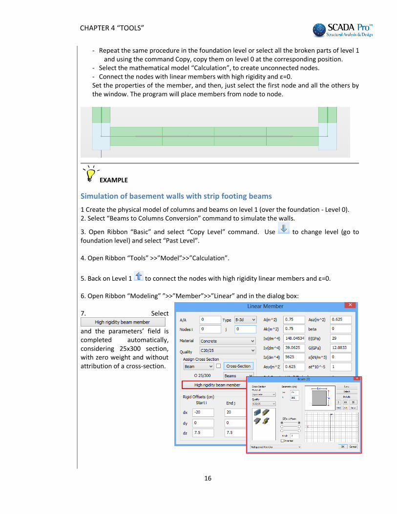
- Repeat the same procedure in the foundation level or select all the broken parts of level 1 and using the command Copy, copy them on level 0 at the corresponding position.

- Select the mathematical model “Calculation”, to create unconnected nodes. - Connect the nodes with linear members with high rigidity and ε=0. Set the properties of the member, and then, just select the first node and all the others by the window. The program will place members from node to node.

EXAMPLE

Simulation of basement walls with strip footing beams

1 Create the physical model of columns and beams on level 1 (over the foundation - Level 0). 2. Select “Beams to Columns Conversion” command to simulate the walls.

3. Open Ribbon “Basic” and select “Copy Level” command. Use to change level (go to foundation level) and select “Past Level”. 4. Open Ribbon “Tools” >>”Model”>>”Calculation”.

5. Back on Level 1 to connect the nodes with high rigidity linear members and ε=0. 6. Open Ribbon “Modeling” ”>>”Member”>>”Linear” and in the dialog box: 7. Select

and the parameters’ field is completed automatically, considering 25x300 section, with zero weight and without attribution of a cross-section.


17

8. Left click to connect the nodes, one by one. You can also use the

following button and connect automatically all the nodes included in the window. 9. Go to Level 0 (foundation). 10. Open Ribbon “View”>>”Display”>>”Switches” and deactivate “Auto Trim”. 11. Open Ribbon “Modeling”>>”Foundation” >>” Strip Footing Beams” and in the following dialog box: - Type the geometry

- Deactivate the checkbox “R. Offsets” 12. Insert the beam from one node to the next one.

3.2.2 Smith Model

According to this method, the wall is modeled with two linear members placed in “X” order. To implement “Model Smith” simulation:

1. Level 1: in the position of the wall put a beam with the same thickness 2. Level 0: put the Strip Footing Beams or Footing Connection Beam 3. Select ”Smith Model” 4. Left click on the beam that is going to change automatically.

The program inserts two linear members in “X” order between two columns and the

parameters A, Ak, Asy, asz, and Iz of the members, on the border of the simulated wall, are changed automatically.


18

3.2.3 Diagonals

Follow the “Smith Model” procedure. Based on the “Diagonals” method, the basement wall is modeled with two linear members placed in “X” order (diagonal order).

The main difference between the Smith Method and the Diagonals is that the second method simulates the wall, without changing the inertial characteristics of the members on the border, unlike the Smith method.

The basic precondition for using these two methods for simulating walls is the presence of the mathematical model and the presence of the beams that will be transformed in X linear members. These beams must have the same thickness as the simulated walls. Automatically the program calculates the rigid offsets of the members.

3.2.4 Rigid Offset Change

The command to define a new position of an elastic node at the beginning or the end of a mathematical member, modifying automatically the rigid offset of the connected member. Beam elastic node is the intersection point between the axis of the beam and the border line of the connected column. Column elastic node is the node at the center of mass of the cross-section. Select the command and the element to change the rigid offset. The program detects the elastic node. Left click to define the new position of the elastic node .

3.2.5 Piles The foundation piles included in the new version of SCADA Pro are circular reinforced concrete piles. Loads are transmitted through the pile tip on the ground while at the same time the lateral friction also works. Superstructure’s loads are transfered by the pile cap (simulated in SCADA Pro with finite surface elements) at the top of each pile and then on the ground.


19

Select the command and the following dialog box appears:

where you specify: The material and the grade.

In the circular cross-section pile, you can also attribute steel quality. However, only reinforced concrete piles will be designed.

Then define the diameter D of the pile and the total Length L. The step has to do with the parts into which the total pile will be split, to create the nodes where the side springs will be placed. Two transport springs will be placed in each node in the two vertical directions x and z. Finally, there is the Layer option to place the piles. Press «Soil Data» to open the dialog box:

where you specify the number of terrain zones and then, for each zone you select from the drop down list "Zone", you specify the data. Place the pile selecting a node from the pile cap.


20

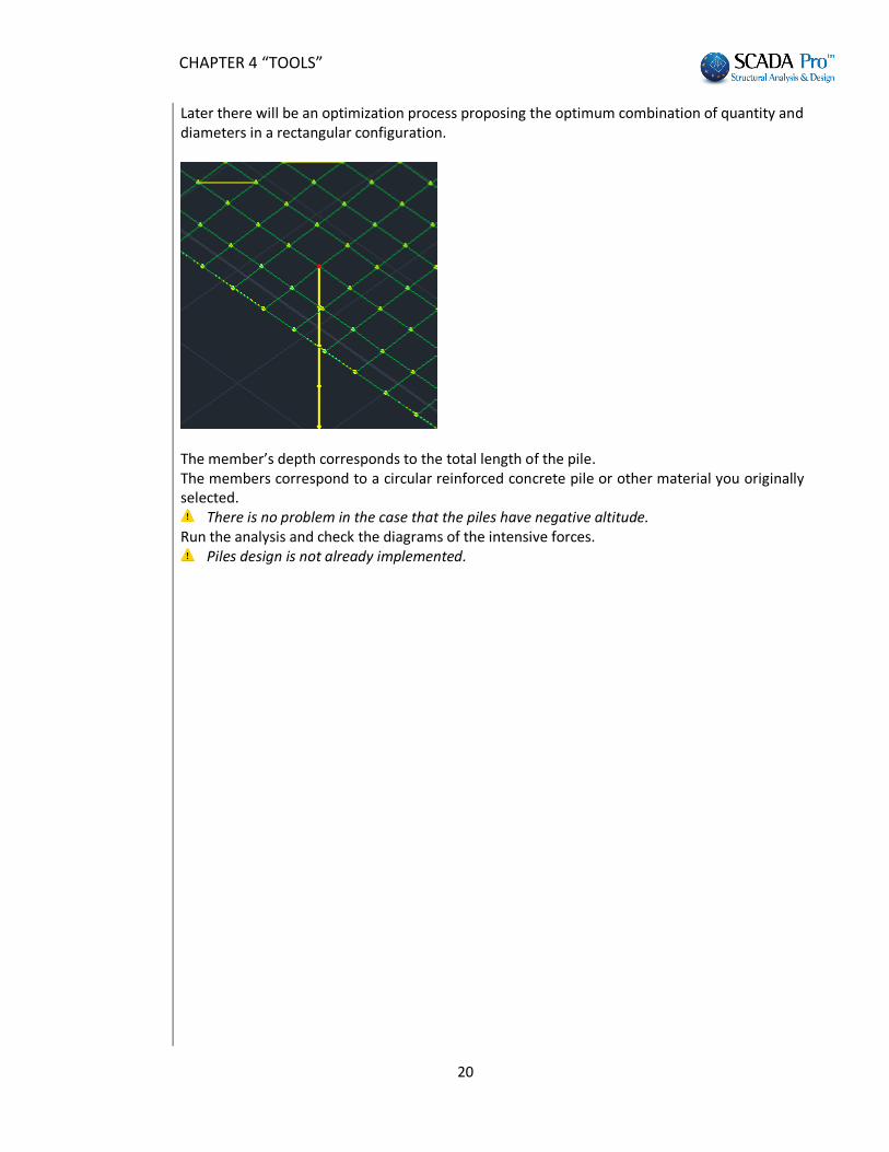
Later there will be an optimization process proposing the optimum combination of quantity and diameters in a rectangular configuration.

The member’s depth corresponds to the total length of the pile. The members correspond to a circular reinforced concrete pile or other material you originally selected.

There is no problem in the case that the piles have negative altitude. Run the analysis and check the diagrams of the intensive forces.

Piles design is not already implemented.


21

4. Members

The command group “Members” contains commands that allow the management and modification of the mathematical members: - Segmentation - Intersection - Change Direction - Direction redefinition - Member’s merging - Beam-Plate Connection

The basic precondition for these commands is that the members have been created using the

command "Modeling >> Elements >> Member >> Linear" with or without section attribution

or using the command "Templates".

4.1 Segmentation

This command allows the discretization of a linear member in individual members according to the number of the members or the length of each member. Select the command and the following dialog box is displayed:

Specify either the number of the segments or the maximum length of each segment. Then press the button “OK” and point the mouse on the member you want to break.

By selecting the command "Auto" all mathematical members of the structure, that intersect, break automatically. This option works only with mathematical members and needs to be used carefully because it breaks all crossing members.

4.2 Intersection

This command allows the segmentation of two linear members which intersect and create four new members and a node on the intersection point.


22

Select the command and the two linear members. The two members break into four members and a new node is created on the intersection point.

4.3 Change Direction:

Use the command to change the direction of the local axis of the members. Enable in "Switches" the Local Axes, select the command and left click on the member. Observe the change in the direction.

4.4 Direction Redefinition:

This command should be used if one or both of the following messages appear in the Model Checks Reports:

Error1678: column 21 has been assigned with the wrong orientation There are members with the wrong local axis

The first one, which is relative only to columns, has to do with the direction of their placement (the correct direction is from the bottom to the top), while the second is a general message concerning beams and columns, and especially for the beams, appears when they are not placed with the program conversion, from left to right and from top to bottom. So when the above messages appear, using the "Direction Redefinition" command the program corrects automatically the orientation for the entire model.


23

4.5 Member Merging

This command allows merging two or more members placed sequentially. The new member preserves the inertial properties of the first one. (Figure a).

Figure a Select the command and point on the mathematical members sequentially by starting always from the first member. The mathematical member obtained has the inertial properties of the first member. Then delete the intermediate nodes (Figure b1, b2).

Figure b1 Figure b2

4.6 Beam-Plate Connection

In a surface discretized with surface elements bounded by linear elements (ex. slab-beams), the connection between the two types of the element must be implemented.

This command works as described below:

First, break the linear member in some parts similar to the elements of the mesh on the edges.

Then, connect the nodes of the linear members with the closer mesh nodes by implementing rigid offsets.

Select the command, left click on the linear member and on the mesh element nodes, one by one or by using the window selection. Alternatively, choose between the following commands:

- Ribbon “Tools” >>”Members”>>” ”. Select border beams one by one and the connection is applied automatically.

- Ribbon “Tools” >> “Members”>>” ”. Just select the command and the program carries out the rest procedure automatically for the current level.


24

5. Nodes

The command group “Nodes” contains commands that allow the management and modification of the mathematical nodes: - Replacement - Coincidence - Beam-Plate Node Coincidence - Beam-Plate Node Constraint - Merge

5.1 Replacement

This command is used to replace one node with another and delete simultaneously the original node. Select the command and the node to be replaced. Then click on the replacement node (Fig. a) The first node is canceled and the member is connected with a rigid offset to the new node (Fig. b).

Fig. a Fig. b

5.2 Coincidence

Select the command and show two or more nodes. The program creates a new node, then cancel the others and connect the members with the new nodes with rigid offsets. Select the command, left click on the nodes and right click to exit the command.


25

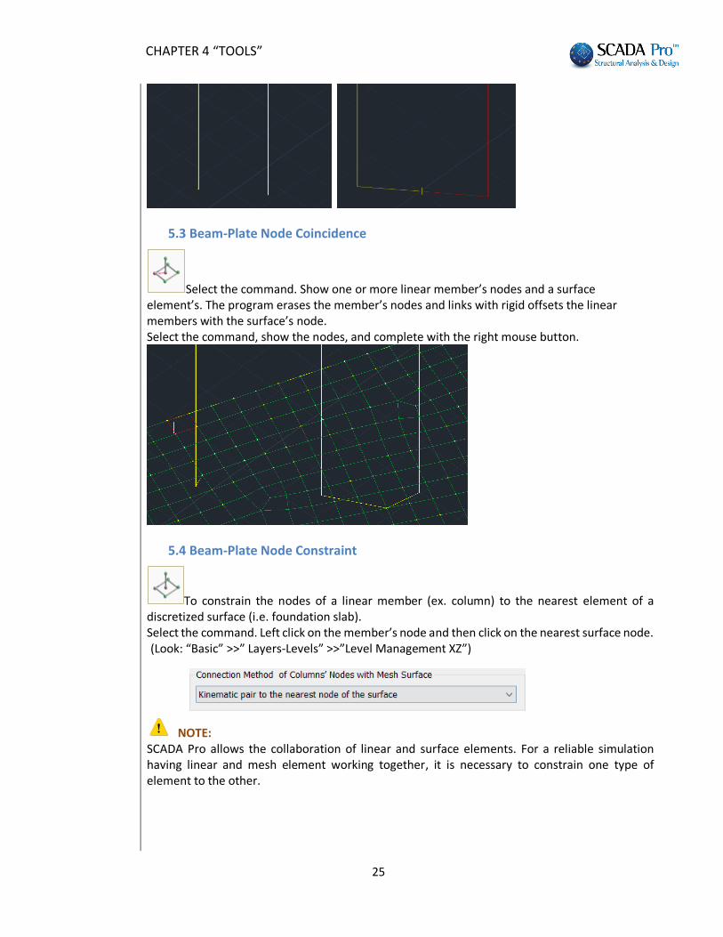
5.3 Beam-Plate Node Coincidence

Select the command. Show one or more linear member’s nodes and a surface element’s. The program erases the member’s nodes and links with rigid offsets the linear members with the surface’s node. Select the command, show the nodes, and complete with the right mouse button.

5.4 Beam-Plate Node Constraint

To constrain the nodes of a linear member (ex. column) to the nearest element of a discretized surface (i.e. foundation slab). Select the command. Left click on the member’s node and then click on the nearest surface node. (Look: “Basic” >>” Layers-Levels” >>”Level Management XZ”)

NOTE: SCADA Pro allows the collaboration of linear and surface elements. For a reliable simulation having linear and mesh element working together, it is necessary to constrain one type of element to the other.


26

5.5 Merge

Command to merge the nodes in small distances between them. Select the command and specify a distance value. Nodes at a distance less or equal to this will be merged, resulting in a single node.

6. Various

The command group "Various" contains the following commands: - Measurement (Length, Angle, Area, Perimeter) - Alignment

6.1 Find Length, Angle

This command is used to find the length, relative distances x, y, and z as well as the angle. Click the first point that defines the beginning. Then, while you move the mouse pointer, you can see on the status bar the distance L, the relative coordinates Dx, Dy and Dz and the angle

. Click the second point to read the relative values.

6.2 Find Area, Perimeter

This command is used to find area and perimeter. Select the command and the tops or the edges of the area. Then right click and in the status line you see the area, the coordinates of the mass center and the perimeter


27

6.3 Alignment

This command is used to align one object to another. Select “Alignment” and an object (e.g. a column) to align. Then select the line (or circle or point) for the alignment.

EXAMPLE 1 Consider the line (e) and the column 80x50. Select “Alignment”.

Left click first on the side (1) of the column and then on line (ε) to receive the first configuration. Left click first on the side (2) of the column and then on line (ε) to receive the second configuration.

EXAMPLE 2 Consider a beam (T1) and two columns (30x60). Select “Alignment”.

Left-click first on one central point of the upper side of the beam and then on the upper part of the two columns. Left-click first on the upper side of the beam, near the left column and on the upper part of left columns. Then left click, again, on the bottom side of the beam, near the right column and on the bottom part of the left column.

EXAMPLE 3 Consider two circular columns and a connection beam.


28

Left click on the upper side of the beam, near the edge (α) and on the column K2 (from (ε’) and further). Then left click, again, on the bottom side of the beam, near the edge (b) and on the column K1 (from (ε’’) and before), to receive the configuration.

6.4 Match Properties

This command allows you to attribute the properties of the object selected in other similar objects. Select the command and left click on an object to open the corresponding window containing the individual properties. Check the properties you want to assign and OK to close the window. Then, select (using any selection tools) similar objects to which you attributed the selected properties of the first object.

the new upgraded interface of scada pro · 2018-07-23 · in the new upgraded scada pro, all...

Documents