�

�

�

�

NOTICE: This is the author’s version of a work that was accepted for publication in Science of ComputerProgramming. Changes resulting from the publishing process, such as peer review, editing, corrections, structuralformatting, and other quality control mechanisms may not be reflected in this document. A definitive versionwas subsequently published in Science of Computer Programming, 64(2007):115-139.

DOI: http://dx.doi.org/10.1016/j.scico.2006.03.009

The Octahedron Abstract Domain

Robert Clariso 1,2

Estudis d’Informatica i MultimediaUniversitat Oberta de Catalunya (UOC)

Barcelona, Spain

Jordi Cortadella 2

Departament de Llenguatges i Sistemes InformaticsUniversitat Politecnica de Catalunya (UPC)

Barcelona, Spain

Abstract

An interesting area in static analysis is the study of numerical properties. Complexproperties can be analyzed using abstract interpretation, provided that an adequateabstract domain is defined. Each domain can represent and manipulate a family ofproperties, providing a different trade-off between the precision and complexity ofthe analysis. The contribution of this paper is a new numerical abstract domaincalled octahedron that represents constraints of the form (

∑xi −

∑xj ≥ k). The

implementation of octahedra is based on a new kind of decision diagrams calledOctahedron Decision Diagrams (OhDD).

Key words: Abstract Interpretation; Numerical Abstract Domains; RelationalAbstract Domains; Convex Polyhedra

1 Part of this research was performed while this author was at the Departament deLlenguatges i Sistemes Informatics of UPC.2 Supported by CICYT TIN 2004-07925 and the FPU grant AP2002-3862 from theSpanish Ministry of Education, Culture and Sports.

Preprint submitted to Elsevier Science 23 November 2006

1 Introduction

Abstract interpretation [9] defines a generic framework for the static analysisof dynamic properties of a system. This framework can be used, for instance,to analyze termination or to discover invariants in programs automatically.However, each analysis requires the framework to be parametrized for therelevant domain of properties being studied, e.g. numerical properties.

There is a wide spectrum of numerical abstract domains that can be used torepresent and manipulate properties. Some examples are intervals, octagonsand convex polyhedra. Each domain provides a different trade-off between theprecision of the properties that can be represented and the efficiency of themanipulation. An interesting problem in abstract interpretation is the studyof new abstract domains that are sufficiently expressive to analyze relevantproblems and allow an efficient implementation.

In this paper, a new numerical abstract domain called the octahedron abstractdomain is described. It can represent conjunctions of restricted linear inequal-ities called unit inequalities, of the form (

∑xi − ∑

xj ≥ k). A new kindof decision diagram called Octahedron Decision Diagram (OhDD) has beenspecifically designed to represent and manipulate this family of constraints ef-ficiently. The implementation of the octahedron abstract domain allows somedegree of optimization when the variables under study are non-negative. Sev-eral classes of interesting problems such as the study of the values of clocksor counters, or the analysis of the length or size of an element (string, list,. . . ) contain non-negative variables, so this optimization can be applied. Someexamples of problems that can be solved using unit inequalities over non-negative variables are the analysis of timed systems [1, 18], the analysis ofstring length in C programs [12] and the discovery of bounds on the size ofasynchronous communication channels. In other problems where variables areunconstrained, OhDD can still be used albeit with lower efficiency.

This paper is an extended version of the conference paper with the same titlepublished in the Static Analysis Symposium (SAS) 2004. In this extendedversion, further details are provided about the following areas: the canonicityof the representation, the implementation of the operations, the use of OhDDwith unrestricted variables and the potential benefits of dynamic reordering.

The remaining sections of the paper are organized as follows. Section 2 presentsrelated work in the definition of numerical domains for abstract interpreta-tion, and previous decision diagram techniques used to represent numericalconstraints. Section 3 defines the numerical domain of octahedra, and Section4 describes the data structure and its operations. This Section will also discussdifferent implementations depending on the class of variables being studied:

2

Table 1A comparison of numerical abstract domains based on inequality properties.

Abstraction Reference Constraints Example

Intervals [9] (k1 ≤ xi ≤ k2) k1, k2 ∈ Q 2 ≤ x ≤ 5

Difference Bound [11, 3] (k1 ≤ xi ≤ k2) k1, k2 ∈ Q 1 ≤ x ≤ 3

Matrices (DBMs) (xi − xj ≤ k) k ∈ Q x− y ≤ 5

Octagons [22] (± xi ± xj ≤ k) k ∈ Q 2 ≤ x + y ≤ 6

Two-variables [30] (c1 · x1 + c2 · x2 ≥ k) 3x− 2y ≥ 5

per-inequality c1, c2, k ∈ Q

Octahedra This paper (∑

xi −∑

xj ≥ k) x + z − y ≥ 5

k ∈ Q

Convex polyhedra [10, 17] (∑

ci · xi ≥ k) x + 3y − z ≥ 1

ci, k ∈ Q

Templates [29] Like convex polyhedra, but the set of

possible coefficients ci is established a priori.

unconstrained variables or non-negative variables. In Section 5, some possi-ble applications of the octahedron abstract domain are discussed, and someexperimental results are presented. Finally, Section 6 draws some conclusionsand suggests some future work.

2 Related Work

2.1 Numerical Abstract Domains

Abstract domain is a concept used to denote a computer representation for afamily of constraints, together with the algorithms to perform the abstractoperators such as union, intersection, widening or transfer functions. Sev-eral abstract domains have been defined for interesting families of numericalproperties, such as inequality , equality or modulo properties. The octahedronabstract domain belongs to the first category, inequalities. Other abstract do-mains based on inequalities are intervals, difference bound matrices, octagons,two-variables-per-inequality , and convex polyhedra. An example of these ab-stract domains and their relation to octahedra can be seen in Table 1.

Intervals are a representation for constraints on the upper or lower bound foreach variable, e.g. (k1 ≤ xi ≤ k2). Interval analysis is very popular due to its

3

simplicity and efficiency: an interval abstraction for n variables requires O(n)space, and all operations require O(n) time in the worst case. Octagons arean efficient representation for a system of inequalities on the sum or differenceof variable pairs, e.g. (±xi±xj ≤ k) and (xi ≤ k). The implementation of oc-tagons is based on difference bound matrices (DBM), a data structure used torepresent constraints on differences of pairs of variables, as in (xi−xj ≤ k) and(xi ≤ k). Efficiency is an advantage of this representation: the spatial cost forrepresenting constraints on n variables is O(n2), while the temporal cost is be-tween O(n2) and O(n3), depending on the operation. Convex polyhedra are anefficient representation for conjunctions of linear inequality constraints. Thisabstraction is very popular due to its ability to express precise constraints.However, this precision comes with a very high complexity overhead, which isunbounded in theory but exponential in practice [10]. This complexity has mo-tivated the definition of abstract domains such as two-variables-per-inequality ,which try to retain the expressiveness of linear inequalities with a lower com-plexity. However, currently there is no experimental data comparing the per-formance or the precision of this abstract domain to that of convex polyhedra,so it is unclear whether the lower theoretical complexity is noticeable from apractical point of view.

The abstract domain presented in this paper, octahedra, also attempts to keepsome of the flexibility of convex polyhedra with a lower complexity. Instead oflimiting the number of variables per inequality, the coefficients of the variablesare restricted to {−1, 0, +1}. From this point of view, octahedra provide aprecision that is between octagons and convex polyhedra. The precision ofoctahedra and the two-variables-per-inequality domain are not comparable.

The abstract domains presented so far are restricted to a specific subclass oflinear inequalities that is established in the definition of the domain. Instead,the domain of template constraints [29] allows the user to define the structureof the properties to be analyzed. This domain has a parameter: a ”template”matrix T describing the potential invariants. This matrix has one column pervariable, and one row for each potential invariant. The value of a position Tij

in this matrix describes the coefficient of the variable xj in the i-th invariant.Then, all the operations of the abstract domain are posed as linear program-ming (LP) problems, using the template matrix to define the constraints ofthe problems. The number of LP problems to be solved is polynomial in termsof the size of the template, i.e. the number of potential invariants.

In some sense, template constraints subsume all the other abstract domainsdescribed in this section. However, the more specialized domains may be moreefficient because they can exploit the structure of the constraints in the im-plementation. Furthermore, the template matrix may be very large, e.g. a(3n − 1)× n matrix for an octahedron with n variables, or even infinite, e.g.in the two-variables-per-inequality domain.

4

2.2 Decision diagrams

One possible implementation of octahedra is based on decision diagrams. De-cision diagram techniques have been applied successfully to several problemsin different application domains. Binary Decision Diagrams (BDD) [5] providean efficient mechanism to represent boolean functions. Zero Suppressed BDDs(ZDD) [21] are specially tuned to represent sparse functions more efficiently.Multi-Terminal Decision Diagrams (MTBDD) [15] represent functions fromboolean variables to reals, f : Bn → R.

The paradigm of decision diagrams has also been applied to the analysis ofnumerical constraints. Most of these approaches compare the value of nu-merical variables with constants or intervals, or compare the value of pairsof variables. Some examples of these representations are Difference DecisionDiagrams (DDD) [23], Region Encoding Diagrams (RED) [35], Numerical De-cision Diagrams (NDD) [13], and Clock Difference Diagrams (CDD) [4]. Al-though the individual constraints involve a maximum of two variables, thesediagrams can encode conjunctions and disjunctions of these constraints. Inother representations, each node encodes one complex constraint like a linearinequality. Some examples of these representations are Decision Diagrams withConstraints (DDC) [19] and Hybrid-Restriction Diagrams (HRD) [36]. Again,these diagrams can encode conjunctions and disjunctions of linear inequalities.Nevertheless, there is no sistematic procedure to combine the different con-straints in the diagram, detect redundancies and simplify the representation.The Octahedron Decision Diagrams described in this paper use an innovativeapproach to encode linear inequalities. This approach, presented in Section4, includes a procedure called saturation that combines and simplifies the in-equalities of the diagram. However, contrary to other decision diagrams, thereis a loss of precision when encoding the disjunction of constraints.

3 Octahedra

3.1 Definitions

The octahedron abstract domain is now introduced. In the same way as convexpolyhedra, an octahedron abstracts a set of vectors in Qn as a system oflinear inequalities satisfied by all these vectors. The difference between convexpolyhedra and octahedra is the family of constraints that are supported.

Definition 1 (Unit linear inequality) A linear inequality is a constraintof the form (c1 ·x1 + . . .+cn ·xn ≥ k) where the coefficients ci are in Q and the

5

x x

y

y

y y

x

y

x

y

x

y

x

x

y

x

(b)

(a)

321 4

Fig. 1. Examples of (a) octahedra and (b) non-octahedra over two variables.

constant term k is in Q ∪ {−∞}, e.g. (3x+2y−z ≥ −7). A linear inequalityis called unit if all coefficients are in {−1, 0, +1}, such as (x + y − z ≥ −7).

Definition 2 (Octahedron) An octahedron O over Qn is the set of solutionsto the system of m unit inequalities O = {X | AX ≥ B }, with the vectorB ∈ (Q ∪ {−∞})m and the matrix A ∈ {−1, 0, +1}m×n. Octahedra satisfy thefollowing properties:

(1) Convexity: An octahedron is a convex set, i.e. any segment between twopoints of the octahedron is fully within the octahedron.

(2) Closed for intersection: The intersection of two octahedra is also an oc-tahedron.

(3) Non-closed for union: In general, the union of two octahedra might not bean octahedron.

Figure 1(a) shows some examples of octahedra in a two-dimensional space. InFig. 1(b) there are several regions of space which are not octahedra, eitherbecause they are not connected (1), they are not convex (2), they cannot berepresented by a finite system of linear inequalities (3), or because they can berepresented as a system of linear inequalities, but not unit linear inequalities(4). Notice that in two-dimensional space all octahedra are octagons; octa-hedra can only show a better precision than octagons in higher-dimensionalspaces.

During the remaining of this paper, we will use C to denote a vector in{−1, 0, +1}n where n is the number of variables. Therefore, given a set ofvariables X, the expression (CT X ≥ k) denotes the unit linear inequality(c1 · x1 + . . . + cn · xn ≥ k).

Lemma 3 An octahedron over n variables can be represented by at most 3n−1non-redundant inequalities.

6

PROOF. Each variable can have at most three different coefficients in a unitlinear inequality. For n variables, there are at most 3n possible combinationsof unit coefficients, where one of them is an irrelevant unit inequality with 0in all coefficients. This means that if an octahedron has more than 3n−1 unitinequalities, some of them will only differ in the constant term, e.g. (CT X ≥k1) and (CT X ≥ k2). One of these inequalities is definitely redundant, namely,the one with the smaller constant. �

A problem when dealing with convex polyhedra and octahedra is the lack ofcanonicity of the systems of linear inequalities: the same polyhedron/octahedroncan be represented with different systems of inequalities. For example, bothsystems of inequalities (x = 3) ∧ (y ≥ 5) and (x = 3) ∧ (x + y ≥ 8) define thesame octahedron with different inequalities. Given a convex polyhedron, thereare algorithms to minimize the number of constraints in a system of inequal-ities, i.e. removing all constraints that can be derived as linear combinationsof others. However, in the previous example both representations are minimaland even then, they are different. Although it is possible to define a canonicalform for convex polyhedra [2], its complexity makes it impractical. Regard-ing octahedra, a canonical form for octahedra can be defined using the resultof Lemma 3. Even though the number of inequalities of this canonical formmakes an explicit representation impractical, symbolic representations basedon decision diagrams can manipulate sets of unit inequalities efficiently.

Definition 4 (Canonical form of octahedra) The canonical form of anoctahedron O ⊆ Qn is either (i) the empty octahedron or (ii) a system of3n − 1 unit linear inequalities, where in each inequality (CT X ≥ k), k is thetightest bound satisfied by O. This bound k may be −∞, i.e. the inequality isunbounded in the octahedron.

Theorem 5 Two octahedra O1 and O2 represent the same subset of Qn if andonly if they both have the same canonical form.

Proof We need to prove both directions of the if and only if. (→) Given aconstraint (CT X ≥ k), there is a single tightest bound to that constraint.Therefore, if two octahedra are equal, they will have the same bound for eachpossible linear constraint, and therefore, the same canonical form. �

(←) From its definition, an octahedron is completely characterized by itssystem of inequalities. If two octahedra O1 and O2 have the same canonicalform, then they satisfy exactly the same system of inequalities and thereforeare equal. �

7

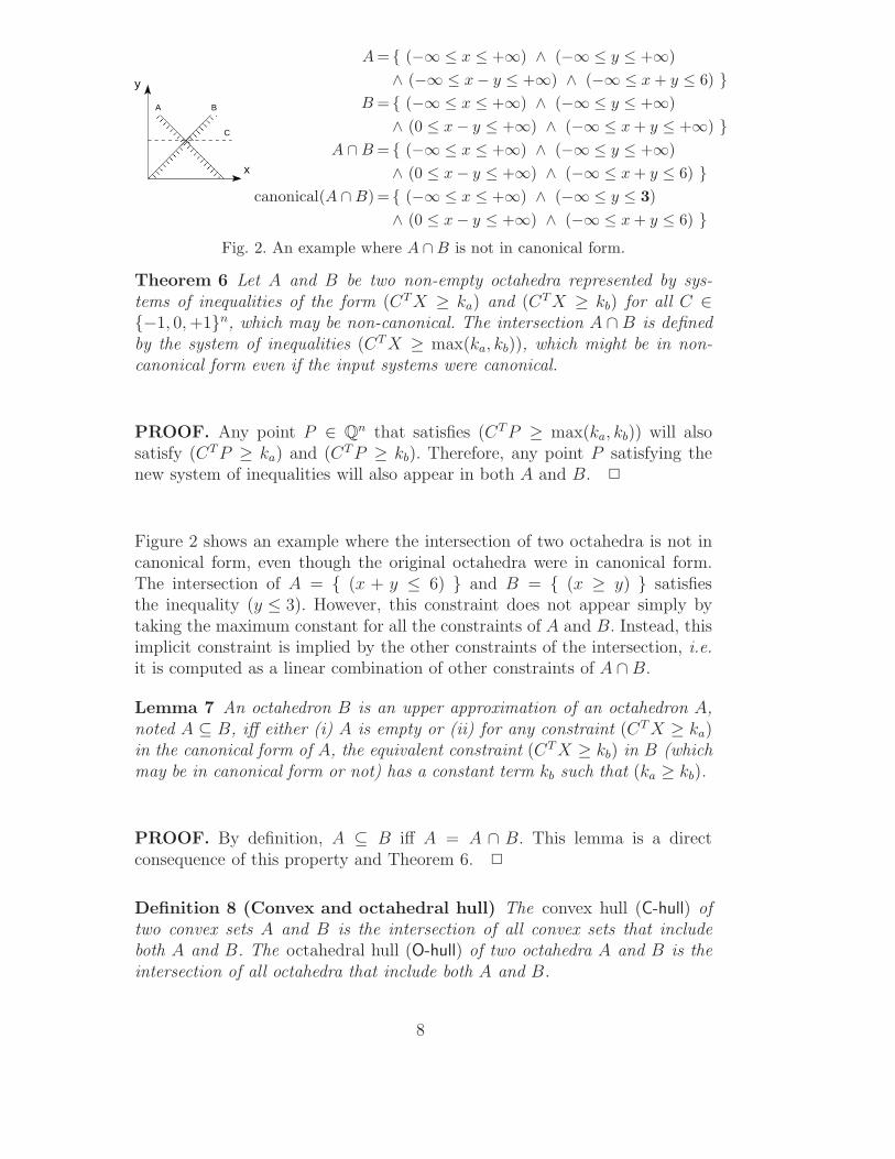
y

x������������������������������

������������������������������

������������������������������

������������������������������

A B

C

A = { (−∞ ≤ x ≤ +∞) ∧ (−∞ ≤ y ≤ +∞)∧ (−∞ ≤ x− y ≤ +∞) ∧ (−∞ ≤ x + y ≤ 6) }

B = { (−∞ ≤ x ≤ +∞) ∧ (−∞ ≤ y ≤ +∞)∧ (0 ≤ x− y ≤ +∞) ∧ (−∞ ≤ x + y ≤ +∞) }

A ∩B = { (−∞ ≤ x ≤ +∞) ∧ (−∞ ≤ y ≤ +∞)∧ (0 ≤ x− y ≤ +∞) ∧ (−∞ ≤ x + y ≤ 6) }

canonical(A ∩B) = { (−∞ ≤ x ≤ +∞) ∧ (−∞ ≤ y ≤ 3)∧ (0 ≤ x− y ≤ +∞) ∧ (−∞ ≤ x + y ≤ 6) }

Fig. 2. An example where A ∩B is not in canonical form.

Theorem 6 Let A and B be two non-empty octahedra represented by sys-tems of inequalities of the form (CTX ≥ ka) and (CTX ≥ kb) for all C ∈{−1, 0, +1}n, which may be non-canonical. The intersection A ∩ B is definedby the system of inequalities (CT X ≥ max(ka, kb)), which might be in non-canonical form even if the input systems were canonical.

PROOF. Any point P ∈ Qn that satisfies (CTP ≥ max(ka, kb)) will alsosatisfy (CT P ≥ ka) and (CT P ≥ kb). Therefore, any point P satisfying thenew system of inequalities will also appear in both A and B. �

Figure 2 shows an example where the intersection of two octahedra is not incanonical form, even though the original octahedra were in canonical form.The intersection of A = { (x + y ≤ 6) } and B = { (x ≥ y) } satisfiesthe inequality (y ≤ 3). However, this constraint does not appear simply bytaking the maximum constant for all the constraints of A and B. Instead, thisimplicit constraint is implied by the other constraints of the intersection, i.e.it is computed as a linear combination of other constraints of A ∩ B.

Lemma 7 An octahedron B is an upper approximation of an octahedron A,noted A ⊆ B, iff either (i) A is empty or (ii) for any constraint (CT X ≥ ka)in the canonical form of A, the equivalent constraint (CT X ≥ kb) in B (whichmay be in canonical form or not) has a constant term kb such that (ka ≥ kb).

PROOF. By definition, A ⊆ B iff A = A ∩ B. This lemma is a directconsequence of this property and Theorem 6. �

Definition 8 (Convex and octahedral hull) The convex hull (C-hull) oftwo convex sets A and B is the intersection of all convex sets that includeboth A and B. The octahedral hull (O-hull) of two octahedra A and B is theintersection of all octahedra that include both A and B.

8

x

y

x

y

x

y

O−hull(A,B)C−hull(A,B)

A U B

B

A

B

A

A

B

A = {(2 ≤ x ≤ 4) ∧ (4 ≤ y ≤ 7)}B = {(1 ≤ x ≤ 5) ∧ (1 ≤ y ≤ 3)}

C-hull = {(1 ≤ x ≤ 5) ∧ (1 ≤ y ≤ 7) ∧(4x− y ≥ 1) ∧ (−4x− y ≥ −23)}

O-hull = {(1 ≤ x ≤ 5) ∧ (1 ≤ y ≤ 7) ∧(x− y ≥ 5) ∧ (−x− y ≥ −11)}

Fig. 3. Overapproximations of the union: convex (C) and octahedral (O) hull.

Figure 3 shows an example of the convex and octahedral hulls of two octahedraA and B. Notice that the convex hull is always an upper approximation ofthe union, and the octahedral hull is always an upper approximation of theconvex hull, i.e. A ∪B ⊆ C-hull(A, B) ⊆ O-hull(A, B).

Theorem 9 Let A and B be two non-empty octahedra whose canonical formare respectively (CT X ≥ ka) and (CTX ≥ kb) for all C ∈ {−1, 0, +1}n.Then, the octahedral hull O-hull(A, B) is defined by the system of inequalities(CT X ≥ min(ka, kb)).

PROOF. Given a bound k for one inequality (CT X ≥ k) of O-hull(A, B),the proof can be split into two parts: proving that k ≤ min(ka, kb) and provingthat k ≥ min(ka, kb).

As the octahedral hull includes A and B, all points P ∈ A and P ∈ B shouldalso be in O-hull(A, B). Therefore, any point in A or B should satisfy theconstraints of O-hull(A, B). Given a constraint (CT X ≥ k), it is known thatpoints in A satisfy (CT X ≥ ka) and points in B satisfy (CTX ≥ kb). If bothsets of points must satisfy the constraint in O-hull(A, B), then k must satisfyk ≤ min(ka, kb).

On the other side, the octahedral hull is the least octahedron that includesA and B. Therefore, the bounds of each constraint should be as tight aspossible, i.e. as large as possible. If we know that k ≤ min(ka, kb) should holdfor a given unit inequality, the tightest bound for that inequality is preciselyk = min(ka, kb). As a corollary , the octahedral hull computed in this way isin canonical form. �

9

y

x

(3, 2)

(3, 3)

(1, 0)

(1, 1)

P

System of generators

P = {λ1 · (3, 3) + λ2 · (3, 2) + µ1 · (1, 1) + µ2 · (1, 0) |λ1 ≥ 0, λ2 ≥ 0, µ1 ≥ 0, µ2 ≥ 0, λ1 + λ2 = 1}

System of constraints

P = {(x, y) | (y ≥ 2) ∧ (x ≥ 3) ∧ (x− y ≥ 0)}Fig. 4. An example of a convex polyhedron (shaded area) and its double description.

3.2 Computing the Canonical Form

3.2.1 Preliminaries: Dual Representations of Polyhedra

Any convex polyhedron has two dual representations: the system of constraintsand the system of generators [6]. The system of constraints defines the poly-hedron as a conjunction of linear inequalities. Meanwhile, the system of gen-erators defines the polyhedron as the convex combination of a set of points(vertices) and the positive linear combination of a set of rays (vectors). Bothrepresentations are useful in the implementation of the abstract domain ofconvex polyhedra, as operations like intersection are trivial in the constraintrepresentation, while the convex hull is naturally expressed in the generatorrepresentation. Also, both representations can be minimized when the dual isavailable. Figure 4 shows an example of a convex polyhedron and its doubledescription.

There is a procedure that translates from one representation into the other.This procedure was described in [6], and further improved in [14, 34]. Givena system of c constraints over Qd, the computation of the dual representationrequires O(c�

d2�) time [20]. Furthermore, even if we consider only minimized

representations, the size of a representation can grow exponentially with thistranslation. For example, an hypercube in d-dimensions is defined by 2d con-straints but it has 2d vertices. The worst case is achieved by cyclic polytopes[20], which have up to O(c�

d2�) vertices with a system of inequalities with c

constraints.

3.2.2 The algorithm

The computation of the canonical form of octahedra will be based on thegenerator representation of the octahedron. The pseudocode for a possible al-gorithm is presented in Figure 6. The output of the algorithm should be eitherthe empty octahedron or the bounds for each of the 3d− 1 unit inequalities ofthe canonical form.

The algorithm is based on the two following observations. First, a ray is a

10

y y

x x

P P

x≥ 3

y≥ 2

x + y≥ 5

x− y≥ 0

(a)

−x≥−∞−y≥−∞

−x− y≥−∞−x + y≥−∞

(b)

Fig. 5. (a) Bounded unit inequalities, (b) unbounded unit inequalities.

vector that represents a direction of unbounded growth in the octahedron,i.e. no constraint can impose a bound that “crosses” the ray. Therefore, aunit inequality will be unbounded in an octahedron O if it crosses one of therays of O. And second, if a unit inequality is bounded, its tightest bound willoccur in one of the vertices of the octahedron. Figure 5 shows an exampleof these observations in the system of generators from Figure 4. All the unitinequalities that cross the rays are unbounded as shown in Fig. 5(b). On theother hand, all the bounded inequalities achieve the tightest bound in one ofthe vertices of the octahedron, as shown in Fig. 5(a).

If a unit inequality is defined as (CT X ≥ k), it is possible to determinewhether it crosses a ray r using the scalar product: if (CT · r < 0), then theunit inequality crosses the ray. For example, the ray (1, 0) is crossed by theinequality (−x + y ≥ k) because (−1, 1)T · (1, 0) = (−1) · 1 + 1 · 0 = −1.Also, given a vertex v, the tightest bound k achieved by a unit inequality(CT X ≥ k) can be computed as k = CT · v. For instance, the bound of theinequality (x−y ≥ k) in a vertex (3, 2) is (1,−1)T · (3, 2) = 1 ·3+(−1) ·2 = 1.

3.2.3 Complexity

For an octahedron over Qd with v vertices and r rays, the algorithm requiresO(d · (v + r) · 3d) time. The space requirement is O(d · (v + r + 3d)) in theworst case. We can establish upper bounds for v and r in terms of d. Forexample, we know that r ≤ 2d as further rays would be redundant in termsof positive linear combinations. With respect to v, a possible upper bound isv ≤ (3d − 1)�

d2�, as there are at most 3d − 1 non-redundant inequalities. It is

possible that a better bound can be established by taking into account thatall constraints are unit inequalities, but currently this is an open problem.

11

Function Canonical form(O)Input: An octahedron O defined as a system of inequalities over d variables.Output: The canonical form of O, which is either the empty octahedron (if O isempty) or the canonical system of 3d − 1 unit inequalities for O.

Compute the system of generators of O: the set of vertices V and rays Rif V = ∅ then

return emptyendif{ Compute the bound of each inequality in the canonical form }for each unit inequality C ∈ {−1, 0,+1}d in O do{ Evaluate the rays for this inequality }unbounded := falsefor each ray r ∈ R do

unbounded := (CT · r < 0)?if unbounded then

breakendif

endforif unbounded then

tightest bound := −∞else{ Evaluate all the vertices for this inequality }{ Keep the tightest bound satisfied by all vertices }tightest bound := +∞for each vertex v ∈ V do

new bound := CT · v{ (CT ·X ≥ new bound) holds for this vertex }tightest bound := min ( new bound, tightest bound ){ (CT ·X ≥ tightest bound) holds for all vertices visited so far }

endforendifbounds[ C ] = tightest bound{ bounds[ C ] = k means (CT ·X ≥ k) }

endforreturn bounds

Fig. 6. Pseudocode to compute the canonical form of an octahedron.

The complexity of these algorithms makes the computation of the canonicalform impractical. Even though the canonical form is useful to define the se-mantics of the operations, it is not practical for the implementation. Instead ofthe canonical form, we will define a relaxed version called the saturated form.Operations performed using the saturated form may lose some precision, while

12

always yielding an upper approximation of the exact result.

3.2.4 Canonicity in other abstract domains

The problem of computing a canonical form appears in other abstract do-mains as well. In domains based on inequality properties, it might be possibleto compute a tighter bound to a constraint by combining several other con-straints. A possible way to compute the canonical form consists in calculatingall possible combinations of constraints.

In the case of DBMs and octagons, only pairwise combinations of constraintsshould be considered. The algorithms that compute the canonical form in theseabstract domains require O(n3) time [11, 22] when variables are rational.

A canonical form for template constraints can also be computed. This com-putation requires solving c linear programming (LP) problems, where c is thenumber of linear inequalities in the template. Given a template for all pos-sible unit constraints, it is also possible to use this method to compute thecanonical form of an octahedron. However, this method requires solving 3d−1LP problems so, like the algorithm presented in this paper, it is impracticalexcept for small values of d.

Convex polyhedra also have a canonical form [2], but the complexity of itscomputation is very high. For instance, it involves discovering all redundantconstraints in the system of inequalities, which can be posed as several LPproblems.

3.3 Abstractions of Octahedra

As it was shown in the previous section, the canonical form of an octahedronprovides a useful mechanism to define operations such as the test for inclu-sion, the intersection or the octahedral hull. However, it is not convenient toimplement the operations using the canonical form.

On the other hand, octahedra are defined in the context of abstract interpre-tation of numerical properties. In this context, the problem is the abstractionof a set of values in Qn, and the main concern is ensuring that the abstractionis an upper approximation of the concrete set of values. Thus, as long as anupper approximation can be guaranteed, an exact representation of octahe-dra is not required, as octahedra are already abstractions of more complexsets. Keeping this fact in mind, efficient algorithms that operate with upperapproximations of the canonical form can be designed.

13

The first step is the definition of a relaxed version of the canonical form,which is called saturated form 3 . While the canonical form has the tightestbound in each of its inequalities, the bounds in the saturated form may bemore relaxed. A system of unit inequalities is in saturated form as long as thebounds imposed by the sum of any pair of constraints in the system appearexplicitly. For example, a saturated form of the octahedron (a ≥ 3)∧ (b ≥ 0)∧(c ≥ 0)∧ (b−c ≥ 7)∧ (a + b ≥ 8)∧ (a + c ≥ 6) can be defined by the followingsystem of inequalities:

(a ≥ 3) ∧ (b ≥ 7) ∧ (c ≥ 0) ∧ (a + b ≥ 10) ∧ (a + c ≥ 6) ∧ (b + c ≥ 7)

∧ (b− c ≥ 7) ∧ (a + b− c ≥ 10) ∧ (a + b + c ≥ 13)

where the constraints with a bound of −∞ have been removed for brevity.In this example, saturation has exposed explicitly that (a + b ≥ 10). Thisinequality is the sum of (a ≥ 3), (b− c ≥ 7) and (c ≥ 0).

A saturated form O∗ of an octahedron O = { X | AX ≥ B } can be computedusing an iterative procedure called saturation. At each step of this procedure,a sum between two unit inequalities is computed. If this sum has a tighterbound than the one already known, the bound is updated, and so on until afixpoint is reached. The formal description of saturation is the following:

(1) Initialize the system of 3n − 1 unit inequalities for all possible valuesof the coefficients C ∈ {−1, 0, +1}n. The bound k of a given inequality(CT X ≥ k) is chosen as:

k =

b if CT X ≥ b appears in AX ≥ B and C �≥ 0n.

−∞ otherwise

(2) Select two inequalities CT1 X ≥ k1 and CT

2 X ≥ k2 such that k1 > −∞and k2 > −∞. Let us define C∗ = C1 + C2 and k∗ = k1 + k2.

(3) If C∗ �∈ {−1, 0, +1}n return to step 2.(4) If CT

∗ X ≥ k appears in the system of inequalities with k ≥ k∗, return tostep 2.

(5) Replace the inequality CT∗ X ≥ k by CT

∗ X ≥ k∗.(6) Repeat steps 2-5 until:• A fixpoint is reached or• An inequality CT

∗ X ≥ k with C = 0n and k > 0 is found. In this case,the octahedron is empty.

3 In the context of a system of constraints, the term saturated is usually used witha different meaning: to denote constraints which cannot become tighter withoutchanging the set of solutions. In this paper we will only use the term to refer to thesaturated form, even though some inequalities in this form may be non-saturated.

14

The implementation of the saturation algorithm will differ slightly from thisdefinition: in step 2, instead of choosing a pair of inequalities and computingthe sum, the implementation will select all possible pairs of unit inequalitiesand compute the sum simultaneously. This operation can be performed effi-ciently in the decision diagram. In any case, it does not affect the terminationof the algorithm.

Theorem 10 Let O = {X | AX ≥ B} be a non-empty octahedron. Thesaturation algorithm applied to O terminates.

PROOF. Each step of the saturation algorithm defines a tighter bound foran inequality of the octahedron. The new inequality (CT

3 X ≥ k′3) is obtained

from two previously known inequalities (CT1 X ≥ k1) and (CT

2 X ≥ k2), so thatC3 = C1 +C2 and k′

3 = k1 +k2, and k′3 > k3, where k3 is the previously known

bound for the inequality. If inequalities 1 and 2 were computed in previousrounds of the saturation algorithm, this dependency chain can be expanded,e.g. if inequality 2 comes from inequalities 4 and 5, then C3 = C1+C4+C5 andk′

3 = k1 + k4 + k5. Non-termination of the saturation algorithm implies thatthere will be infinitely many sums of pairs of inequalities. Ignoring the bound k,there are only finitely many inequalities over n variables. Therefore, it is alwayspossible to find a step that computes a bound k′

j that depends on a previouslyknown bound kj , i.e. Cj = Cj+

∑Cl and k′

j = kj+∑

kl. As Cj−Cj =∑

Cl = 0n

and k′j − kj =

∑kl > 0, the linear combination ((

∑Cl)

T X ≥ (∑

kl)) isequivalent to (0 > 0), which implies that O is empty. �

The fixpoint in saturation may not be reached if the octahedron is empty.For example, the octahedron in Fig. 7(a) is empty because the sum of thelast four inequalities is (0 ≥ 4). The saturation algorithm applied to thisoctahedron does not terminate. Adding the constraints in top-down orderallows the saturation algorithm to produce (x2 − x4 ≥ 5), which can again beused to produce (x2−x4 ≥ 9) and so on. Even then, the saturation algorithmis used to perform the emptiness test because of three reasons:

• There are special kinds of octahedra for which termination is guaranteed.For instance, if all inequalities describe constraints between symbols (allconstant terms are zero), saturation is guaranteed to terminate. This occursbecause any sum among unit constraints will either leave a constant as 0,or replace a −∞ constant by a 0.• The conditions required to build an octahedron for which the saturation al-

gorithm does not terminate are complex and artificial, and therefore we ex-pect them to occur rarely in practical examples. Note that non-terminationmay arise only for some systems of unit inequalities that define an emptyoctahedron.

15

• Another reason is the good behavior of the saturation procedure in practi-cal examples. If the input is an octahedron obtained by performing minorchanges to previously saturated octahedra, e.g. the intersection of two sat-urated octahedra, typically very few iterations are required to reach thefixpoint. This makes the prediction of non-termination possible in practice.

Even if the saturation algorithm terminates, in some cases it might fail todiscover the tightest bound for an inequality. For example, in the octahedronin Fig. 7(b), saturation will fail to discover the constraint (x1−x2+x3+x4+x5+x6 ≥ 6), as any sum of two inequalities will yield a non-unit linear inequality.Therefore, given a constraint (CT X ≥ ks) in the saturated form, the bound kc

for the same inequality in the canonical form may be different, kc �≤ ks. Butkc ≥ ks always holds, as kc is the tightest bound for that inequality. In thissense, the result will always be an upper approximation of the exact canonicalresult, as kc ≥ ks is the exact definition for upper approximation of octahedra(Lemma 7)

Several operations which have been defined for the canonical form can also beused in the saturated form. For instance, the definition of the intersection inTheorem 6 did not require that the operands were in canonical form. Regardingthe union, we were able to prove in Theorem 9 that the octahedral hull is incanonical form if the two initial octahedra are in canonical form. A similarresult holds for octahedra in saturated form.

Lemma 11 Given two octahedra A and B in saturated form, the union im-plemented as (CT X ≥ min(ka, kb)) is also saturated.

PROOF. The result can only be non-saturated if we can find three inequal-ities (CT

1 X ≥ k1), (CT2 X ≥ k2) and (CT

3 X ≥ k3) such that the first twocan be combined to produce the third (C1 + C2 = C3) with a tighter bound(k1 + k2 > k3). Considering the relationship between these bounds and thebounds of A and B in the same inequalities C1, C2 and C3, we can definek1 = min(ka

1 , kb1), k2 = min(ka

2 , kb2), k3 = min(ka

3 , kb3). As A is saturated, we

know that (ka3 ≥ ka

1 + ka2), and conversely for B, (kb

3 ≥ kb1 + kb

2). Therefore, weknow that k3 = min(ka

3 , kb3) ≥ min(ka

1 +ka2 , k

b1 +kb

2). Proving that the result issaturated is then reduced to checking that (k1 + k2 ≤ k3), which is equivalentto: min(ka

1 , kb1) + min(ka

2 , kb2) ≤ min(ka

1 + ka2 , k

b1 + kb

2). This property can bechecked using a proof by cases. �

16

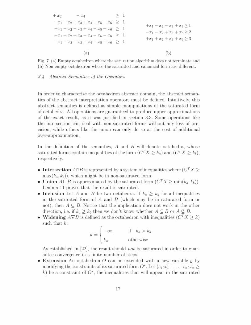
+ x2 − x4 ≥ 1−x1 − x2 + x3 + x4 + x5 − x6 ≥ 1+x1 − x2 − x3 + x4 − x5 + x6 ≥ 1+x1 + x2 + x3 − x4 − x5 − x6 ≥ 1−x1 + x2 − x3 − x4 + x5 + x6 ≥ 1

+x1 − x2 − x3 + x4≥ 1−x1 − x2 + x3 + x5≥ 2+x1 + x2 + x3 + x6≥ 3

(a) (b)

Fig. 7. (a) Empty octahedron where the saturation algorithm does not terminate and(b) Non-empty octahedron where the saturated and canonical form are different.

3.4 Abstract Semantics of the Operators

In order to characterize the octahedron abstract domain, the abstract seman-tics of the abstract interpretation operators must be defined. Intuitively, thisabstract semantics is defined as simple manipulations of the saturated formof octahedra. All operations are guaranteed to produce upper approximationsof the exact result, as it was justified in section 3.3. Some operations likethe intersection can deal with non-saturated forms without any loss of pre-cision, while others like the union can only do so at the cost of additionalover-approximation.

In the definition of the semantics, A and B will denote octahedra, whosesaturated forms contain inequalities of the form (CT X ≥ ka) and (CT X ≥ kb),respectively.

• Intersection A∩B is represented by a system of inequalities where (CT X ≥max(ka, kb)), which might be in non-saturated form.• Union A∪B is approximated by the saturated form (CTX ≥ min(ka, kb)).

Lemma 11 proves that the result is saturated.• Inclusion Let A and B be two octahedra. If ka ≥ kb for all inequalities

in the saturated form of A and B (which may be in saturated form ornot), then A ⊆ B. Notice that the implication does not work in the otherdirection, i.e. if ka �≥ kb then we don’t know whether A ⊆ B or A �⊆ B.• Widening A∇B is defined as the octahedron with inequalities (CT X ≥ k)

such that k:

k =

−∞ if ka > kb

ka otherwise

As established in [22], the result should not be saturated in order to guar-antee convergence in a finite number of steps.• Extension An octahedron O can be extended with a new variable y by

modifying the constraints of its saturated form O∗. Let (c1 ·x1+. . .+cn ·xn ≥k) be a constraint of O∗, the inequalities that will appear in the saturated

17

form of the extension are:

c1 · x1 + . . . + cn · xn − 1 · y ≥ −∞c1 · x1 + . . . + cn · xn + 0 · y ≥ k

c1 · x1 + . . . + cn · xn + 1 · y ≥ −∞If the new variable is known to be non-negative, the last constraint can bechanged to a more precise (c1 · x1 + . . . + cn · xn + 1 · y ≥ k) as the knownbound k cannot be decreased by adding a non-negative value.• Projection A projection of an octahedron O removing a dimension xi can

be performed by removing from its saturated form O∗ all inequalities wherexi has a coefficient that is not zero.• Unit linear assignment A unit linear assignment [xi :=

∑mj=1 cj ·xj ] with

coefficients ci ∈ {−1, 0, +1} can be defined using the following steps:· Extend the octahedron with a new variable t.· Intersect the octahedron with the octahedron (t =

∑mj=1 cj · xj)

· Project the variable xi.· Rename t as xi.

3.5 Impact of the conservative inclusion test

Several operations defined using the saturated form cause a loss of precisionbecause they do not use the tightest possible bound in each inequality. Thisloss of precision is always an upper approximation: the most precise result isincluded in the octahedron produced by the operators. In the context of ab-stract interpretation, upper approximations are acceptable: instead of studyingthe exact set of states of a system, an upper approximation of state space iscomputed. A possible way to perform this computation is called increasingchain: initially, our state space S0 only contains the initial states. Each it-eration after the first attempts to discover new reachable states that can beaccessed from previously reached states. The new states are added to statespace, which grows after each iteration: (S0 ⊆ S1 ⊆ S2 ⊆ . . .). The analysisterminates when a fixpoint is reached, i.e. when Si+1 ⊆ Si.

However, the inclusion operator defined for saturated forms is not accurate:even if A ⊆ B, the answer may be inconclusive when the saturation procedurefails to discover the tightest bound for an inequality. In this section, we discusswhether this has any effect on the termination of an abstract interpretationanalysis. Our claim is that even with this inclusion operator, the analysis canbe guaranteed to terminate, even though there may be a loss of precision.

Let us consider the following scenario: after the iteration i+1 of an increasinganalysis, the fixpoint Si+1 ⊆ Si has been reached but the test of inclusion doesnot give a conclusive answer. In this situation, there must be one constraint

18

(CT X ≥ k) in the solutions such that ki+1 < ki, where kj is the bound of theinequality in Sj . The saturated form of Si+1 is unable to compute the tightestbound ki for that inequality. However, after another iteration (i+2), the statespace Si+2 will satisfy Si+1 ⊆ Si+2, because the analysis is an increasing hain.Therefore, the coefficient ki+2 will always be ki+2 ≤ ki+1. Hence, in Si+2 itdoes not matter that the saturated form is unable to compute the tightestbound for (CT X ≥ k). We can conclude that the analysis will terminate, eventhough more iterations may be required. However, in practical examples, thistheoretical scenario does not seem to arise, as constraints tend to be generatedin a structured way that allows saturation to obtain good approximations ofthe exact canonical form.

4 Octahedra Decision Diagrams

4.1 Overview

The constraints of an octahedron can be represented compactly using a spe-cially devised decision diagram representation. This representation is calledOctahedron Decision Diagram (OhDD). Intuitively, it can be described as aMulti-Terminal Zero-Suppressed Ternary Decision Diagram:

• Ternary : Each non-terminal node represents a variable xi and has threeoutput arcs, labelled as {−1, 0, +1}. Each arc represents a coefficient of xi

in a linear constraint.• Multi-Terminal [15]: Terminal nodes can be constants in R ∪ {−∞}. The

semantics of a path σ from the root to a terminal node k is the linearconstraint (c1 · x1 + c2 · x2 + . . . + cn · xn ≥ k), where ci is the coefficient ofthe arc taken from the variable xi in the path σ.• Zero-Suppressed [21]: If a variable does not appear in any linear constraint,

it also does not appear in the OhDD. This is achieved by using specialreduction rules as it is done in Zero-Suppressed Decision Diagrams.

The reduction rules of decision diagrams have an essential role: ensuring thatthe representation is canonical and efficient. In the context of octahedra,canonicity means that saturated octahedra with the same system of inequali-ties are encoded by the same OhDD. Furthermore, a careful choice of reductionrules may decrease the size of the decision diagram, improving both memoryand CPU time for all operations. In the case of OhDD, two reduction rules aredefined: one for octahedra with unbounded variables and another speciallytuned for octahedra with non-negative variables. In both cases, the overallmanipulation of OhDD is the same, with only small changes in the implemen-tation. These issues will be described in detail in the following section.

19

−3

z

0

−

−,0,+

+

x

y

0

−

−0+

0,+

z

2

x≥ 2

y≥ 0

z≥ 0

x + y≥ 3

x− z≥ 2

x + y − z≥ 2

x + y + z≥ 3

Fig. 8. An example of a OhDD. On the right, the constraints of the octahedron.

Figure 8 shows an example of an OhDD and the octahedron it represents onthe right, using reduction rules for non-negative variables. The shadowed pathhighlights one constraint of the octahedron, (x + y − z ≥ 2). All constraintsthat end in a terminal node with −∞ represent constraints with an unknownbound, such as (x− y ≥ −∞). As the OhDD represents the saturated form ofthe octahedron, some redundant constraints such as (x + y + z ≥ 3) appearexplicitly.

This representation based on decision diagrams provides three main advan-tages. First, decision diagrams provide many opportunities for reuse. For ex-ample, nodes in a OhDD can be shared. Furthermore, different OhDD canshare internal nodes, leading to a greater reduction in the memory usage.Second, the reduction rules avoid representing the zero coefficients of the lin-ear inequalities. Finally, symbolic algorithms on OhDD can deal with sets ofinequalities instead of one inequality at a time. All these factors combinedimprove the efficiency of operations with octahedra.

4.2 Definitions

Definition 12 (Octahedron Decision Diagram - OhDD) An OctahedronDecision Diagram is a tuple (V, G) where V is a finite set of positive real-valuedvariables, and G = (N ∪ K, E) is a labeled single rooted directed acyclic graphwith the following properties. Each node in K, the set of terminal nodes, islabeled with a constant in Q ∪ {−∞}, and has no outgoing arcs. Each noden ∈ N is labeled with a variable v(n) ∈ V , and it has three outgoing arcs,labeled −, 0 and +.

By establishing an order among the variables of the OhDD, the notion of or-dered OhDD can be defined. The intuitive meaning of ordered is the same asin BDDs, that is, in every path from the root to the terminal nodes, the vari-ables of the decision diagram always appear in the same order. For example,the OhDD in Fig. 8 is an ordered OhDD.

20

−

D

D

0,+ −

v

zero coefficient

reduction

−

A B C

0 +

v

X Y

− − 0 + +

A B C

v v

0

X Y

−

A B C

0 +

v

X Y

− − 0 + +

A B C

v v

0

X Y

−

Disomorphic subgraph

reduction

isomorphic subgraph

reduction

D

v

zero coefficient

reduction0 −,+(a)

(b)

Fig. 9. Reduction rules: (a) Unconstrained variables, (b) non-negative variables.

Definition 13 (Ordered OhDD) Let � be a total order on the variables Vof a OhDD. The OhDD is ordered if, for any node n ∈ N , all of its descendantsd ∈ N satisfy v(d) � v(n).

In the same way, the notion of a reduced OhDD can be introduced. However,the reduction rules will be different in order to take advantage of the structureof the constraints. In an octahedron, most variables will not appear in allthe constraints. Avoiding the representation of these variables with a zerocoefficient would improve the efficiency of OhDD. This can be achieved as inZDDs by using a special reduction rule.

Let us consider an octahedron like (x− y ≥ 4). Other variables, e.g. z, do notaffect the bound of the constraint. For example, as there is no informationabout z, constraints that involve x, y and z will have a bound like −∞, like(x − y + z ≥ −∞) or (x − y − z ≥ −∞). This scenario can be described asfollows: there is a node n in the OhDD with a variable z, where the outgoingarcs − and + point towards −∞, and the 0 arc points to a node m. In thiscase, the node n can be replaced by node m to avoid encoding the irrelevantvariable z. This reduction rule is displayed in Figure 9(a).

If the variables are known to be non-negative, the reduction rule can be refined.For example, in the case of a constraint like (x − y ≥ 4) and an irrelevantvariable z, the constraints where the variable z appears are (x − y + z ≥ 4)and (x−y−z ≥ −∞). Contrary to the previous case with arbitrary variables,the constraint (x− y + z ≥ 4) has now a known bound as (z ≥ 0). Therefore,the reduction rule should be rephrased to take into account this information:there should be a node n in the OhDD with a variable z, where the outgoingarc − points to −∞ and both the 0 and + arcs point to a node m. Then, thenode n can be replaced by m. Figure 9(b) depicts this alternative reductionrule. Remarkably, using this reduction rule, the set of constraints stating that“any sum of variables is greater or equal to zero” is represented as the singleterminal node 0.

Figure 9 shows an example of the two alternatives, together with the otherreduction rule, which merges isomorphic subgraphs of the decision diagram.

21

(x ≥ 0) ∧ (y ≥ 0) ∧ (z ≥ 0) ∧ (x + y ≥ 3) ∧ (x + z ≥ 3)

x

y

z

− 0

z

y

− 0 3 − 3

z

−

− −

0,+− − +

00,+

+− 0

0 0,+−

+− −

x

z

y

− 0 3

0

− 3

−

− +

0

0

+− 0

− +

x

y

−

z

y

z

− 0

z

y

− 0 3 − 3

z

−,0,+ 0,+− − +

0−0,+

+− 0

−

0 0,+−

+−,0,+

(a)

(b) (c)

Fig. 10. Comparison of reduction rules. On the top, the octahedron being encoded.On the bottom, (a) OhDD with reduction rule 1 - isomorphic subgraphs, (b) OhDDwith reduction rule 2 - unconstrained variables and (c) OhDD with reduction rule3 - non-negative variables.

Notice that contrary to BDDs, nodes where all arcs have the same target willnot be reduced (unless the three arcs point to −∞). It is possible to haveboth types of variables in the same OhDD, using the suitable reduction rulefor each variable.

Definition 14 (Reduced OhDD) A reduced OhDD is an ordered OhDD wherenone of the following rules can be applied:

(1) Reduction of isomorphic subgraphs: Let D1 and D2 be two isomorphicsubgraphs of the OhDD. Merge D1 and D2.

(2) Reduction of zero coefficients (with unconstrained variables): Let n ∈ Nbe a node with the − and + arcs going to the terminal −∞, and with thearc 0 pointing to a node m. Replace n by m. Or

(3) Reduction of zero coefficients (with non-negative variables): Let n ∈ Nbe a node with the − arc going to the terminal −∞, and with the arcs 0and + pointing to a node m. Replace n by m.

22

Figure 10 shows the effect of the different reduction rules on a OhDD. Inthis case, the octahedron being represented is (x ≥ 0) ∧ (y ≥ 0) ∧ (z ≥ 0) ∧(x + y ≥ 3)∧(x + z ≥ 3). The detection of isomorphic subgraphs is illustratedin Figure 10(a). To improve the clarity of the Figure, terminal nodes with thesame constant value have not been collapsed into a single node. As all thevariables in this example are non-negative, the two alternative reduction rules2 and 3 can be compared, as shown in Figures 10(b) and (c). Notice thatthe reduction that assumes non-negative variables produces a more compactrepresentation. Therefore, whenever all the variables in a problem are known tobe non-negative, reduction rule number 3 should be used instead of reductionrule number 2.

4.3 Implementation of the Operations

The octahedra abstract domain and its operations have been implemented asOhDD on top of the CUDD decision diagram package [32]. Each operation onoctahedra performs simple manipulations such as computing the maximumor the minimum between two systems of inequalities, where each inequality isencoded as a path in a OhDD.

Two concepts from BDDs are used to present the implementation of the op-erations. First, the top variable of a OhDD is the variable that appears in theroot of the OhDD. Two OhDD may have different top variables, because somevariables are not encoded when the reduction rules are applied. Given severalordered OhDD, the top variable among all of them is the one which appearsbefore in the ordering. The other concept is the term cofactor from Booleanalgebra. The two cofactors of a Boolean formula f(x1, . . . , xn) : Bn → B arethe pair of formulas obtained by replacing variable xi by constants 0 and 1respectively inside f . In a BDD, the cofactors of a node f with respect tothe top variable are the two children of f . In the context of OhDD, the termcofactor is also used to denote the children of a node. Each node f of thedecision diagram has three cofactors f−, f 0 and f+ with respect to a variablex. Each cofactor denotes the set of inequalities in f where the variable x has agiven coefficient, i.e. f 0 contains all the inequalities where x does not appear.The cofactors of a OhDD f with respect to the top variable are the targetsof the three arcs −, 0 and +, while the cofactors for the other variables aredefined by the chosen reduction rule.

The operations on octahedra can be implemented as recursive procedures on aOhDD. The algorithm may take as arguments one or more decision diagrams,depending on the operation. All these recursive algorithms share the sameoverall structure:

23

(1) Check if the call is a terminal case, e.g. all arguments are constant decisiondiagrams. In that case, the result can be computed directly.

(2) Look up the cache to see if the result of this call was computed previouslyand is available. In that case, return the precomputed result.

(3) Select the top variable t in all the arguments according to the ordering.The algorithm will only consider this variable during this call, leaving therest of the variables to be handled by the subsequent recursive calls.

(4) Obtain the cofactors of t in each of the arguments of the call.(5) Perform recursive calls on the cofactors of t.(6) Combine the results of the different calls into the new top node for vari-

able t.(7) Store the result of this recursive call in the cache. Future calls to this

method with the same arguments will use the cached result instead ofrepeating the computation.

(8) Return the result to the caller.

The saturation algorithm is a special case: all sums of pairs of constraintsare computed by a single traversal; but if new inequalities have been discov-ered, the traversal must be repeated. The process continues until a fixpoint isreached. Even though this fixpoint might not be reached, as seen in Fig. 7, thenumber of iterations required to saturate an octahedron tends to be very low(1-4 iterations) if it is derived from saturated octahedra, e.g. the intersectionof two saturated octahedra.

These traversals might have to visit 3n inequalities/paths in the OhDD in theworst case. However, as OhDD are directed graphs, many paths share nodes somany recursive calls will have been computed previously, and the results willbe reused without the need to recompute. The efficiency of the operations ondecision diagrams depends upon two very important factors. The first one isthe order of the variables in the decision diagram. Intuitively, each call shouldperform as much work as possible. Therefore, the variables that appear earlyin the decision diagram should discriminate the result as much as possible. Asecond factor in the performance of these algorithms is the effectivity of thecache to reuse previously computed results.

4.3.1 Reduction rules

In order to implement the reduction rules, two basic operations should bedefined. First, how to obtain the OhDD for the three cofactors (coefficients)of a given variable. And second, how to build a new OhDD from the threecofactors of a given variable. Figure 11 shows the pseudocode for these twoprocedures, called DD GetCofactors and DD CombineCofactors.

The only remarkable aspect of DD GetCofactors is how to compute the cofac-

24

Function DD GetCofactors(var, f)Input: An OhDD f over non-negative variables and a variable var. If var appearsin the decision diagram f , it must appear as the top variable.Output: The 3 cofactors of f for variable var, < f−, f0, f+ >.

if DD IsConstant(f) ∨ DD TopVariable(f) �= var then< f−, f0, f+ > := < −∞, f, f >

else< f−, f0, f+ > := < DD NegArc(f), DD ZeroArc(f), DD PosArc(f) >

endifreturn < f−, f0, f+ >

Function DD CombineCofactors(var, f−, f0, f+)Input: The three cofactors of a OhDD for a given variable var. Any variable inthe cofactors must appear after var in the ordering.Output: A OhDD where < f−, f0, f+ > are the three cofactors for variable var.

if f0 = f+ ∧ f− = −∞ thenreturn f0

elsereturn DD UniqueNode(var, f−, f0, f+)

endif

Fig. 11. Implementation of the reduction rules for non-negative variables.

tors of a variable that does not appear in a OhDD. If a variable is missing, itmeans that it has been reduced. In a OhDD with non-negative variables, thismeans that its negative cofactor is −∞ while its positive and zero cofactor areequal to the OhDD. A similar implementation produces the reduction rules forunconstrained variables.

Regarding DD CombineCofactors , its pseudocode assumes that there is a pro-cedure called DD UniqueNode that detects isomorphic nodes in the decisiondiagram, so if an isomorphic node already exists it is returned, otherwise anew one is created instead. This operation is typically provided by all decisiondiagram packages [5].

4.3.2 Saturation

The saturation procedure can be implemented symbolically. Instead of choos-ing two constraints and computing its linear combination, the linear combi-nation of a whole set of constraints is computed in one step. Figures 12 and13 show the pseudocode that performs this saturation.

25

Function Saturate(f)Input: A OhDD f .Output: The saturation of the OhDD f .

doold := fres := SaturateRecur(f , f)f := MaximumRecur(f , res){ Emptiness test - find a constraint (0 ≥ k) with (k > 0) }aux := fwhile ¬DD IsConstant(aux) do

aux := DD ZeroArc(aux)endwhileif aux > 0 then return +∞ endif

until f = oldreturn res

Fig. 12. Pseudocode of the saturation procedure and the emptiness test.

The recursive saturation algorithm SaturateRecur computes the linear combi-nation of its two parameters. Intuitively, the computation is split according tothe top variable of the decision diagram. The only cases relevant to our compu-tation are those where the top variable will have a coefficient in {−1, 0, +1} inthe result of the linear combination. For example, the linear combination hasa coefficient +1 if one of the arguments has coefficient 0 and the other has co-efficient +1. The remaining variables of the linear combination are computedrecursively using the same algorithm.

Saturation is performed by computing these linear combinations and addingthem to the system of inequalities until a fixpoint is reached. This compu-tation is described in the procedure Saturate in Figure 12. Notice that aftercomputing each set of linear combinations, they are added to the OhDD usingthe maximum operator, which in OhDD corresponds to the intersection. If aconstraint of the form (0 ≥ k) with (k > 0) appears during the computationof the fixpoint, then we know that the octahedron is empty.

In order to encode the empty octahedron, an additional terminal node is usedin our implementation: +∞. This terminal was not presented in Definition 12to separate the concept of OhDD from implementation issues. Intuitively, anyconstraint with a constant term of +∞, i.e. (±x1 ± . . .± xn ≥ +∞) is false,so the semantics of the decision diagram is preserved. Moreover, choosing thisterminal node to encode empty octahedra is also natural in the following sense:

26

Function SaturateRecur(f , g)Input: Two OhDD called f and g.Output: The OhDD describing the pairwise linear combinations of f and g, ignoringconstraints with a coefficient outside {−1, 0,+1}.

{ Terminal cases }if DD IsConstant(f) ∧ DD IsConstant(g) then

return DD Sum(f , g)endifif f = +∞ ∨ g = +∞ then return +∞ endifif f = −∞ ∨ g = −∞ then return −∞ endif

{ Lookup the result in the cache }res := DD CacheLookup(SaturateRecur, f , g)if res �= null then return res endiftop := DD TopVariable(f , g)< f−, f0, f+ > := DD GetCofactors(top, f)< g−, g0, g+ > := DD GetCofactors(top, g)

{ The shorthand MAX(a,b) is used instead of MaximumRecur(a,b) }

{ Recursive calls for top coefficient = −1 }res− := MAX( SaturateRecur(f−, g0), SaturateRecur(f0, g−) )

{ Recursive calls for top coefficient = 0 }res0 := MAX( MAX( SaturateRecur(f0, g0), SaturateRecur(f+, g−) ),

SaturateRecur(f−, g+) )

{ Recursive calls for top coefficient = +1 }res+ := MAX( SaturateRecur(f+, g0), SaturateRecur(f0, g+) )

{ Combine the cofactors and update the cache }res := DD CombineCofactors(top, res−, res0, res+)DD CacheInsert(SaturateRecur, f , g, res)return res

Fig. 13. Pseudocode of one iteration of the saturation procedure.

• Neutral element of the union: The union is implemented using the minimumoperator so +∞ is the neutral element.• Absorbent element of the intersection: The intersection is implemented using

the maximum operator so +∞ is the absorbent element.

It would also have been possible to encode empty octahedra in a different

27

Function MaximumRecur(f , g)Input: Two OhDD called f and g.Output: An OhDD that has, at the bottom of each path from the root to theterminal nodes, the maximum terminal found in the same path in f and g.

{ Terminal cases }if f = g then return f endifif f = +∞ ∨ g = −∞ then return f endifif f = −∞ ∨ g = +∞ then return g endifif DD IsConstant(f) ∧ DD IsConstant(g) then

return DD Max(f , g)endif

{ Lookup the result in the cache }res := DD CacheLookup(MaximumRecur, f , g)if (res �= null) then return res endif

{ Recursive calls for each cofactor }top := DD TopVariable(f , g)< f−, f0, f+ > := DD GetCofactors(top, f)< g−, g0, g+ > := DD GetCofactors(top, g)

{ The shorthand MAX(a,b) is used instead of MaximumRecur(a,b) }<res−, res0, res+ > := < MAX(f−, g−), MAX(f0, g0), MAX(f+, g+) >

{ Combine the cofactors and update the cache }res := DD CombineCofactors(top, res−, res0, res+)DD CacheInsert(MaximumRecur, f , g, res)return res

Function Intersection(f , g)Input: Two OhDD called f and g.Output: The intersection of f and g.

res := MaximumRecur(f , g)return Saturate(res)

Fig. 14. Pseudocode of the intersection procedure.

way, i.e. adding a boolean variable to OhDD stating whether the octahedron isempty or not. Our approach was chosen for convenience in the implementationof the operations.

28

Function ProjRecur(f , v)Input: A OhDD called f and a variable v.Output: An OhDD that is equal to f except in all nodes labeled with variable v.If there is a node labeled with variable v inside f , it is replaced in the result byone of its children, the one targeted by the arc labeled with coefficient 0.

{ Terminal cases }if DD IsConstant(f) then return f endif

top := DD TopVariable(f);< f−, f0, f+ > := DD GetCofactors(top, f){ Test if this is the variable to be projected }if v = top then return f0 endif{ Test if v precedes top in the top-down variable order. }if v ≤ top then{ Variable v does not appear inside f , it should have appeared before. }return f

endif

{ Lookup the result in the cache }res := DD CacheLookup(MaximumRecur, f , v)if res �= null then return res endif

{ Recursive calls for each cofactor }< res−, res0, res+ > := < ProjRecur(f−, v), ProjRecur(f0, v), ProjRecur(f+, v) >

{ Combine the cofactors and update the cache }res := DD CombineCofactors(top, res−, res0, res+)DD CacheInsert(MaximumRecur, f , g, res)return res

Function Projection(f , v)Input: A OhDD called f and a variable v.Output: The OhDD computed from f after projecting variable v. The projection ofthis variables ”forgets” all the constraints where the variable has a coefficient otherthan zero.

{ Assumption: f is in saturated form. Otherwise we should saturate it here. }res := ProjectRecur(f , g)return Saturate(res)

Fig. 15. Pseudocode of the projection procedure.

29

4.3.3 Other operations

The intersection of two octahedra has been defined as the union of the setsof constraints of both octahedra, choosing the maximum constant for thoseconstraints that appear in both octahedra. In a OhDD, constraints that donot appear in an octahedron are represented by the terminal −∞. Therefore,the intersection of OhDD can be implemented by taking the maximum of thetwo arguments for each path between the root and the terminal nodes. Thepseudocode that computes this maximum is shown in Fig. 14. The result ofthis operation is not necessarily saturated.

The same concept can be applied to the union of octahedra. The union can becomputed as the minimum of the two arguments for each path between theroot and the terminal nodes.

The projection can also be implemented symbolically, as it is shown in Figure15. The concept behind the implementation is the following: this operationshould remove all inequalities where a variable v has a non-zero coefficient.Any inequality where v has a non-zero coefficient will appear in the OhDDas a node labeled with that variable. These nodes have a child, the target ofthe arc labeled with 0, that represents the inequalities where v appears witha coefficient 0. Therefore, the implementation of projection can be summa-rized as follows: traverse the OhDD until a node n labeled with variable v isdiscovered; replace the reference to n with a reference to n0.

Extension, adding a new variable to a OhDD that does not participate inany inequality, is a trivial operation due to the choice of the reduction rules.Both the reduction rules for unconstrained and non-negative variables detectvariables which do not participate in an inequality and remove them from thediagram. Therefore, extending a OhDD with a new variable does not changethe diagram in any way; we only need to decide the position of the new variablein the top-down variable order.

Other operations can be defined similarly or be rewritten in terms of theintersection and the union. For instance, an approximate inclusion test (f ⊆g)? can be rewritten as (f = f∩g)?, using an intersection plus an equality test,which compares whether the top nodes of the decision diagram are equal.

30

5 Applications of the Octahedron Abstract Domain

5.1 Motivating Application

Asynchronous circuits [24] are a class of circuits where there is no globalclock to synchronize its different components. Asynchronous circuits replacethe global clock by a local handshake between components, gaining severaladvantages such as lower power consumption. However, the absence of a clockmakes the verification of asynchronous circuits more complex, since the cor-rectness of the circuit is more dependent on timing constraints. This meansthat the correctness of the circuit depends on the delays of its gates and wires.

In many asynchronous circuits implementing control logic, the timing con-straints that arise are unit inequalities. Intuitively, they correspond to con-straints of the type

(δ1 + · · ·+ δi︸ ︷︷ ︸delay(path1)

)− (δi+1 + · · ·+ δn︸ ︷︷ ︸delay(path2)

) ≥ k

indicating that certain paths in the circuit must be longer than other paths.In very rare occasions, coefficients different from ±1 are necessary. A typicalcounterexample would be a circuit where one path must be c times longerthan another one, e.g. a fast counter.

Figure 16(a) depicts a D flip-flop [27]. Briefly stated, a D flip-flop is a 1-bitregister. It stores the data value in signal D whenever there is a rising edgein the clock signal CK. The output Q of the circuit is the value which wasstored in the last clock rising edge. We would like to characterize the behaviorof this circuit in terms of the internal gate delays. The flip-flop has to becharacterized with respect to three parameters (see Figure 16(b)):

• Setup time, noted as Tsetup, is the amount of time that D should remainstable before a clock rising edge.• Hold time, noted as Thold , is the amount of time that D should remain stable

after a clock rising edge.• Delay or clock-to-output time, noted as TCK→Q , is the amount of time re-

quired by the latch to propagate a change in the input D to the outputQ.

The timing analysis algorithm is capable of deriving a set of sufficient linearconstraints that guarantee the correctness of the circuit’s behavior. This be-havior will be correct if the output Q matches the value of D in the last clockrising edge. Formally, this property can be stated as:

31

T setup T hold

T CK −> Q

HIT

T LO

(a) (b)

CK

D

Qg1

g2g3

g4

CK

Q

DTCK→Q ≤ D2 + D3 + D4

Tsetup > D1 + D2 − d2

Thold > D2 + D3

THI > D2 + D3 + D4

THI > Thold

TLO > Tsetup

d1 > D2

(c)

Fig. 16. (a) Implementation of a D flip-flop [27], (b) description of variables thatcharacterize any D flip-flop and (c) sufficient constraints for correctness for anydelay of the gates.

The value of Q after a delay TCK→Q from CK ’s rising edge must be equalto the value of D CK’s rising edge.

Any behavior not fulfilling this property is considered to be a failure. Fig. 16(c)reports the set of sufficient timing constraints derived by the algorithm. Eachgate gi has a symbolic delay in the interval [di, Di]. Notice that the timingconstraints are unit inequalities.

Timing verification has been performed on several asynchronous circuits fromthe literature. This verification can be seen as the analysis of a set of clockvariables, and the underlying timing behavior can be modeled as assignmentsand guards on these variables [7]. The analysis of clock variables has beenperformed using two different numerical abstractions: convex polyhedra andoctahedra. The implementation of polyhedra uses the New Polka polyhedralibrary [26], while the library of OhDD is implemented on top of the CUDDpackage [32]. Table 2 shows a comparison of the experimental results for someexamples. All these examples were verified successfully using both octahedraand polyhedra, as all relevant constraints were unit linear inequalities. For allthese cases, the execution time of convex polyhedra and octahedra is com-parable, while the memory usage for octahedra is lower. For each example,we provide the number of different states (configurations) of the circuit, thenumber of clock and delay variables of the abstractions and the execution timerequired by the analysis with each abstraction.

The difference in memory usage is quantified in the next example, an asynchro-nous pipeline with different number of stages and an environment running at afixed frequency. The processing time required by each stage i has a processingtime bounded by an interval, with unknown upper and lower bound [di, Di].Whenever a stage finishes its computation, it sends the result to the nextstage if it is empty. The safety property being verified in this case was “theenvironment will never have to wait before sending new data to the pipeline”,i.e. whenever the environment sends new data to the pipeline, the first stage

32

Table 2Experimental results using convex polyhedra and octahedra.

# of # of Polyhedra OhDD

Example States variables CPU Memory CPU Memory

nowick 60 30 0.5s 82Mb 0.1s 9Mb

sbuf-read-ctl 74 31 1.2s 83Mb 1.4s 10Mb

rcv-setup 72 27 2.1s 83Mb 8.3s 21Mb

alloc-outbound 82 39 1.3s 83Mb 0.2s 10Mb

ebergen 83 27 1.3s 83Mb 1.7s 11Mb

mp-forward-pkt 194 29 1.9s 85Mb 3.8s 20Mb

chu133 288 26 1.3s 85Mb 1.0s 13Mb

is empty. Fig.17 shows the pipeline, with an example of a correct and incor-rect behavior. The tool discovers that correct behavior can be ensured if thefollowing holds:

dIN > D1 ∧ . . . ∧ dIN > DN ∧ dIN > DOUT

where Di is the delay of stage i, and dIN and DOUT refer to environmentdelays. This property is equivalent to:

dIN > max(D1, . . . , DN , DOUT )

Therefore, the pipeline is correct if the environment is slower than the sloweststage of the pipeline. Both the polyhedra and octahedra abstract domain areable to discover this property. This example is interesting because it exhibitsa very high degree of concurrency. The verification times and memory usagefor different lengths of the pipeline can be found in Table 3. Notice thatthe memory consumption of OhDD is lower than that of convex polyhedra.This reduction in memory usage is sufficient to verify larger pipelines (n = 6stages) not verifiable with our convex polyhedra implementation. Using convexpolyhedra, the verification tool runs out of memory. Memory usage remainsrelatively low during the execution (about 450Mb) but reaches a peak of morethan 1.7Gb after 8 hours of CPU time; the peak in memory usage occursduring one of the transformations between dual representations of polyhedra.However, the reduction in memory usage achieved by octahedra comes at theexpense of an increase in the execution time, which is spent minimizing thedecision diagrams.

33

Table 3Experimental results for the pipeline example.

# of # of # of Polyhedra OhDD

stages States variables CPU Time Memory CPU Time Memory

2 36 20 0.6s 64Mb 1.0s 5Mb

3 108 24 2.0s 67Mb 17.0s 8Mb

4 324 28 13.5s 79Mb 4m 9.0s 39Mb

5 972 32 4m 19.2s 147Mb 1h 6m 14.0s 57Mb

6 2916 36 – – 39h 44m 18.0s 83Mb

ack

req

ack

reqIN

ack

req OUT

(b)

(c)

(a)

Fig. 17. (a) Asynchronous pipeline with N=3 stages, (b) correct behavior of thepipeline and (c) incorrect behavior. Dots represent data elements.

5.2 Additional experiments

The experimental results presented so far have been computed with OhDDusing the reduction rules for non-negative variables (NNV). Also, a predefinedtop-down variable order has been used. The order for variables has been chosenmanually, where the variables which are likely to appear in many constraintsare placed near the top of the diagram. In this section, we illustrate the per-fomance of OhDD with different settings. The example used to perform thecomparison is the asynchronous pipeline depicted in Figure 17.

For the first comparison, we have implemented the reduction rules for uncon-strained variables (UV) discussed in Section 4.2. This change affects a verysmall part of the implementation, namely the methods GetCofactors and Com-bineCofactors which have been presented in Figure 11. Intuitively, these reduc-tion rules should have a worse performance in problems where variables maybe non-negative, as they cannot avoid representing constraints like (x1 ≥ 0)or (x1 + x2 ≥ 0) explicitly. Table 4 shows the experimental results with thesealternative reduction rules. These results confirm the intuition: the decisiondiagrams using the UV rules are larger, using more memory and requiringmore CPU time to be traversed. The difference becomes more noticeable asthe number of variables becomes larger, because the number of redundant in-equalities grows exponentially with the number of variables. For instance, in asystem with three non-negative variables that satisfy (x1−x2 ≥ 3) the follow-

34

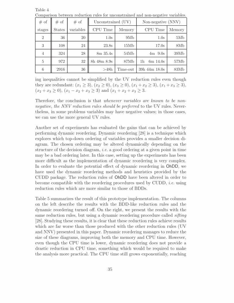
Table 4Comparison between reduction rules for unconstrained and non-negative variables.

# of # of # of Unconstrained (UV) Non-negative (NNV)

stages States variables CPU Time Memory CPU Time Memory

2 36 20 1.0s 9Mb 1.0s 5Mb

3 108 24 23.8s 15Mb 17.0s 8Mb

4 324 28 8m 35.4s 54Mb 4m 9.0s 39Mb

5 972 32 8h 48m 8.9s 87Mb 1h 6m 14.0s 57Mb

6 2916 36 >48h Time-out 39h 44m 18.0s 83Mb

ing inequalities cannot be simplified by the UV reduction rules even thoughthey are redundant: (x1 ≥ 3), (x2 ≥ 0), (x3 ≥ 0), (x1 +x2 ≥ 3), (x1 +x3 ≥ 3),(x2 + x3 ≥ 0), (x1 − x2 + x3 ≥ 3) and (x1 + x2 + x3 ≥ 3.

Therefore, the conclusion is that whenever variables are known to be non-negative, the NNV reduction rules should be preferred to the UV rules. Never-theless, in some problems variables may have negative values; in those cases,we can use the more general UV rules.

Another set of experiments has evaluated the gains that can be achieved byperforming dynamic reordering. Dynamic reordering [28] is a technique whichexplores which top-down ordering of variables provides a smaller decision di-agram. The chosen ordering may be altered dynamically depending on thestructure of the decision diagram, i.e. a good ordering at a given point in timemay be a bad ordering later. In this case, setting up the experiments has beenmore difficult as the implementation of dynamic reordering is very complex.In order to evaluate the potential effect of dynamic reordering in OhDD, wehave used the dynamic reordering methods and heuristics provided by theCUDD package. The reduction rules of OhDD have been altered in order tobecome compatible with the reordering procedures used by CUDD, i.e. usingreduction rules which are more similar to those of BDDs.

Table 5 summarizes the result of this prototype implementation. The columnson the left describe the results with the BDD-like reduction rules and thedynamic reordering turned off. On the right, we present the results with thesame reduction rules, but using a dynamic reordering procedure called sifting[28]. Studying these results, it is clear that these reduction rules achieve resultswhich are far worse than those produced with the other reduction rules (UVand NNV) presented in this paper. Dynamic reordering manages to reduce thesize of these diagrams, improving both the memory and CPU time. However,even though the CPU time is lower, dynamic reordering does not provide adrastic reduction in CPU time, something which would be required to makethe analysis more practical. The CPU time still grows exponentially, reaching

35

Table 5Evaluation of dynamic reordering in OhDD using the CUDD package.

# of # of # of No reordering Dynamic reordering

stages States variables CPU Time Memory CPU Time Memory

2 36 20 1.2s 6Mb 1.0s 5Mb

3 108 24 34.7s 16Mb 25.2s 8Mb

4 324 28 13m 19.4s 55Mb 7m 1.7s 39Mb

5 972 32 > 12h Time-out 7h 14m 14.0s 57Mb

unacceptable values very quickly. The reason behind the low gains achievedwith dynamic reordering seems to be that the initial order chosen for thevariables of the OhDD was good, due to our knowledge about the kind ofconstraints likely to appear in the analysis of a timed system. Nevertheless,the improvements achieved in other applications where a good ordering cannotbe established a priori may be relevant enough to make dynamic reorderingan essential feature of OhDD.

5.3 Other Applications

In general, the octahedron abstract domain may be interesting in any analysisproblem where convex polyhedra can be used. Many times, the precision ob-tained with convex polyhedra is very good, but the efficiency of the analysislimits the applicability. In these scenarios, using octahedra might be adequateas long as unit linear inequalities provide sufficient information for the specificproblem. If the variables involved in the analysis are positive, the suitabilityof octahedra becomes even more noticeable. Some examples of areas of appli-cations are the following:

• Static discovery of bounds in the size of asynchronous communication chan-nels : Many systems communicate using a non-blocking semantics, wherethe sender does not wait until the receiver is ready to read the message. Inthese systems, each channel requires a buffer to store the pending messages.Allocating these buffers statically would improve performance but it is notpossible, as the amount of pending messages during execution is not knownin advance. Analysis with octahedra could discover these bounds statically.The analysis of the bounds of these channels can be performed using octa-hedra. Furthermore, the size of a channel is always positive, so the reductionrule for non-negative variables can be used in the analysis. This problem isrelated to the problem of structural boundedness of a Petri Net [25], wherean upper bound on the number of tokens that can be in each place of thePetri Net must be found.

36

• Analysis of timed systems: Clocks and delays are restricted to positive valuesin many types of models. Octahedra can be used to analyze these valuesand discover complex properties such as timing constraints or worst-caseexecution time (WCET).• Analysis of string length in programs [12]: Checking the absence of buffer

overflows is important in many scenarios, specially in the applications wheresecurity is critical, e.g. an operating system. C programs are prone to er-rors related to the manipulation of strings. Several useful constraints on thelength of strings can be represented with octahedra. For instance, a con-straint on the concatenation of two strings can be strlen(strcat(s1, s2)) =strlen(s1) + strlen(s2).• Analysis of term size in logic programs [33], which can be used among other

things to prove termination of logic programs [31].• Proof of mutual exclusion and other synchronization properties among con-

current processes: many high-level synchronization constraints can be ex-pressed easily as properties on counter (semaphore) variables [16]. For in-stance, mutual exclusion among n processes can be represented with con-straints like (x1 + . . . + xn ≤ 1), where xi = 1 if the process i is inside thecritical section, and xi = 0 otherwise.

6 Conclusions and future work

A new numerical abstract domain called octahedron has been presented. Thisdomain can represent and manipulate constraints on the sum or differenceof an arbitrary number of variables. In terms of precision, this abstraction isbetween octagons and convex polyhedra. Regarding complexity, the worst casecomplexity of octahedra operations over n variables is O(3n) in memory, andO(3n) in execution time in addition to the cost of saturation. However, worst-case performance is misleading due to the use of a decision diagram approach.For instance, BDDs have a worst-case complexity of O(2n), but they have avery good behavior in many real examples. Performance in this case dependson factors such as the ordering of the variables in the decision diagram, theeffectiveness of the cache and the nature of the problem to be solved. Inthe experimental results of OhDD, memory consumption was shown to besmaller than that of our convex polyhedra implementation. Running time wascomparable to that of convex polyhedra in small and medium-sized examples,while in more complex examples the execution time was worse. This showsthat OhDD trade speed for a reduction in memory usage. Dynamic reorderingcan be used to improve both memory and time, but only by a small margin.

Future work in this area will try to improve the execution time of octahedraoperations. An area where there is room for improvement is the current bot-tleneck of the representation, the saturation procedure. Another direction of

37

research is the design of alternative implementations of the octahedron ab-stract domain. For instance, as the set of coefficients is limited and small,each unit inequality can be stored efficiently using bit-vectors. Experimentalresults using a bit-vector implementation have been reported in [8].

Acknowledgements

The authors would like to thank the referees for their insightful commentswhich have enhanced the final version of this paper.

References

[1] R. Alur and D. L. Dill. A theory of timed automata. Theoretical ComputerScience, 126(2):183–235, 1994.

[2] D. Avis, K. Fukuda, and S. Picozzi. On canonical representations ofconvex polyhedra. In Proc. Int. Conf on Mathematical Software, pages350–360. World Scientific, 2002.

[3] R. Bagnara. Data-Flow Analysis for Constraint Logic-Based Languages.PhD thesis, University of Pisa, 1997.

[4] G. Behrmann, K. G. Larsen, J. Pearson, C. Weise, and W. Yi. Efficienttimed reachability analysis using clock difference diagrams. In Proc. In-ternational Conference on Computer Aided Verification, pages 341–353,1999.

[5] R. E. Bryant. Graph-based algorithms for Boolean function manipulation.IEEE Transactions on Computers, C-35(8):677–691, 1986.

[6] N. Chernikova. Algoritm for discovering the set of all solutions of alinear programming problem. U.S.S.R. Computational Mathematics andMathematical Physics, 6(8):282–293, 1964.

[7] R. Clariso and J. Cortadella. Verification of timed circuits with symbolicdelays. In Proc. of Asia and South Pacific Design Automation Conference,pages 628–633, 2004.

[8] R. Clariso and J. Cortadella. Verification of concurrent systems withparametric delays using octahedra. In Proc. International Conferenceon Application of Concurrency to System Design, pages 122–131. IEEEComputer Society Press, 2005.

[9] P. Cousot and R. Cousot. Abstract interpretation: a unified lattice modelfor static analysis of programs by construction or approximation of fix-points. In Proc. of the ACM Symposium on Principles of ProgrammingLanguages, pages 238–252. ACM Press, 1977.

[10] P. Cousot and N. Halbwachs. Automatic discovery of linear restraints

38

among variables of a program. In Proc. of the ACM Symposium on Prin-ciples of Programming Languages, pages 84–97. ACM Press, 1978.

[11] D. L. Dill. Timing assumptions and verification of finite-state concurrentsystems. In Automatic Verification Methods for Finite State Systems,LNCS 407, pages 197–212. Springer-Verlag, 1989.

[12] N. Dor, M. Rodeh, and M. Sagiv. CSSV: towards a realistic tool for stat-ically detecting all buffer overflows in C. In Proc. of the ACM SIGPLANConference on Programming Language Design and Implementation, pages155–167. ACM Press, 2003.

[13] E. Asarin, M. Bozga, A. Kerbrat, O. Maler, M. Pnueli, and A. Rasse. Datastructures for the verification of timed automata. In Hybrid and Real-Time Systems, pages 346–360, Grenoble, France, 1997. Springer Verlag,LNCS 1201.

[14] F. Fernandez and P. Quinton. Extension of Chernikova’s algorithm forsolving general mixed linear programming problems. Technical Report437, IRISA, 1988.

[15] M. Fujita, P. C. McGeer, and J. C.-Y. Yang. Multi-terminal binary de-cision diagrams: An efficient data structure for matrix representation.Formal Methods in System Design, 10(2/3):149–169, 1997.

[16] A. J. Gerber. Process synchronization by counter variables. SIGOPSOperating Systems Review, 11(4):6–17, 1977.

[17] N. Halbwachs, Y.-E. Proy, and P. Roumanoff. Verification of real-timesystems using linear relation analysis. Formal Methods in System Design,11(2):157–185, 1997.

[18] T. A. Henzinger. The Temporal Specification and Verification of Real-Time Systems. PhD thesis, Stanford University, 1991.

[19] C. Mauras. Symbolic simulation of interpreted automata. In 3rd Work-shop on Synchronous Programming, 1996.

[20] P. McMullen. The maximum number of faces of a convex polytope. Math-ematica, (17):179–184, 1970.

[21] S. Minato. Zero-supressed BDDs for set manipulation in combinatorialproblems. In Proc. ACM/IEEE Design Automation Conference, pages272–277. ACM Press, 1993.

[22] A. Mine. The octagon abstract domain. In Proc. of Analysis, Slicing andTranformation (in Working Conference on Reverse Engineering), pages310–319. IEEE CS Press, 2001.

[23] J. Møller, J. Lichtenberg, H. R. Andersen, and H. Hulgaard. Differencedecision diagrams. In Computer Science Logic, The IT University ofCopenhagen, 1999.

[24] D. Muller and W. Bartky. A theory of asynchronous circuits. In Proc. In-ternational Symposium on the Theory of Switching, pages 204–243. Hard-ware University Press, 1959.

[25] T. Murata. State equation, controllability and maximal matchings ofPetri nets. IEEE Transactions on Automatic Control, AC-22(3):412–416,1977.

39

[26] New Polka: Convex Polyhedra Library.http://www.irisa.fr/prive/bjeannet/newpolka.html.

[27] C. Piguet et al. Memory element of the Master-Slave latch type, con-structed by CMOS technology. US Patent 5,748,522, 1998.

[28] R. Rudell. Dynamic variable ordering for ordered binary decision dia-grams. In Proc. International Conference on Computer-Aided Design,pages 42–47. IEEE Computer Society Press, 1993.

[29] S. Sankaranarayanan, H. Sipma, and Z. Manna. Scalable analysis oflinear systems using mathematical programming. In Proc. of Interna-tional Conference on Verification, Model Checking and Abstract Interpre-tation, number 3385 in Lecture Notes in Computer Science, pages 21–47.Springer-Verlag, 2005.

[30] A. Simon, A. King, and J. M. Howe. Two Variables per Linear Inequalityas an Abstract Domain. In Proc. of Logic Based Program Developmentand Transformation, LNCS 2664, pages 71–89. Springer-Verlag, 2002.

[31] K. Sohn and A. Van Gelder. Termination detection in logic programs us-ing argument sizes (extended abstract). In Proc. of the ACM Symposiumon Principles of Database Systems, pages 216–226. ACM Press, 1991.

[32] F. Somenzi. CUDD: Colorado university decision diagram package. Avail-able online at http://vlsi.colorado.edu/~fabio/CUDD.

[33] A. van Gelder. Deriving constraints among argument sizes in logic pro-grams (extended abstract). In Proc. of the ACM Symposium on Principlesof Database Systems, pages 47–60. ACM Press, 1990.

[34] H. L. Verge. A note on Chernikova’s algorithm. Technical Report 635,IRISA, 1992.

[35] F. Wang. Efficient data structure for fully symbolic verification of real-time software systems. In Proc. of Tools and Algorithms for Constructionand Analysis of Systems, pages 157–171. Springer-Verlag, 2000.

[36] F. Wang. Symbolic parametric safety analysis of linear hybrid systemswith BDD-like data-structures. In Proc. International Conference onComputer Aided Verification. Springer-Verlag, 2004.

40