the of critical › pdf › hep-th › 9507044.pdfhep-th/9507044 7 jul 95 the sp ectrum of critical...
TRANSCRIPT

hep-
th/9
5070
44
7 Ju
l 95
The spectrum of critical exponents
in (
~
�
2
)
2
{theory in d = 4� � dimensions
| Resolution of degeneracies
and hierarchical structures
Stefan K. Kehrein
�
Institut f�ur Theoretische Physik,
Ruprecht{Karls{Universit�at,
D-69120 Heidelberg, Germany
June 18, 1995
Abstract
The spectrum of critical exponents of the N{vector model in 4� � di-
mensions is investigated to the second order in �. A generic class of
one{loop degeneracies that has been reported in a previous work is
lifted in two{loop order. One{ and two{loop results lead to the conjec-
ture that the spectrum possesses a remarkable hierarchical structure:
The naive sum of any two anomalous dimensions generates a limit point
in the spectrum, an anomalous dimension plus a limit point generates
a limit point of limit points and so on. An in�nite hierarchy of such
limit points can be observed in the spectrum.
�
E{mail: [email protected]
1

1 Introduction
Relatively little is known about properties of the spectrum of critical exponents in
d > 2 dimensional �eld theories. Conformal symmetry yields insu�cient constraints for
exact solutions in d > 2 dimensions and one has to rely on perturbation expansions. In two
recent publications [6, 7] we have therefore studied the spectrum of critical exponents of the
full operator algebra of composite operators in the critical N{vector model in d = 4 � � di-
mensions in the �{expansion. In one{loop order, a solution of the spectrum problem in terms
of an operator V of anomalous dimensions could be given. The diagonalization of V is a stan-
dard exercise, though it is still nontrivial to make general statements about the spectrum [7].
For an alternative approach and further information about the spectrum see also ref. [3].
Somehow surprising was the result derived from V that there exists an in�nite degeneracy
in the spectrum of non{derivative composite operators. That is an in�nite number of non{
derivative eigenoperators (quasiprimary operators
1
) have vanishing anomalous dimensions in
order �. In fact, in a sense made precise in ref. [7], for a given number of elementary �elds
in the composite operator and an increasing number of gradients, the one{loop spectrum of
anomalous dimensions is dominated by this eigenvalue zero. This raised the question about
the nature of these degeneracies.
In order to address this question in this paper, the one{loop calculation is extended to
two{loop order for a particularly interesting subalgebra C
sym
of the full operator algebra.
Again one can derive a spectrum{generating operator that encodes all the information about
two{loop eigenoperators and anomalous dimensions in C
sym
. The generic case will turn out
to be the resolution of the one{loop degeneracies in two{loop order.
In combination with the previous results in one{loop order, this leads to the observation
of a remarkable structure of limit points in the spectrum: One notices that the sum of any
two eigenvalues in the spectrum generates a limit point in the spectrum. In this manner a
naive sum rule for anomalous dimensions is recovered that generates limit points. Though
this is essentially a conjecture, it can be proven explicitly for a small number of �elds and is
numerically very well supported in the general case. An interesting hierarchical structure of
the spectrum follows naturally from this conjecture consisting of limit points of limit points
of . . . (and so on).
The structure of this paper is as follows. In section 2 we brie y sum up the one{loop
results from our previous papers [6, 7] that are relevant for the purpose of this work. The
calculation in extended to two{loop order in section 3. Using our notion of a spectrum{
1
We use the term \quasiprimary" in analogy to 2d CFTs for non{derivative eigenoperators, that is these
operators are not the total spatial derivative of another operator. Clearly it is not possible to extend the
concept of primary operators in a similar manner for d > 2.
1

generating operator, it is straightforward to obtain eigenoperators and critical exponents in
two{loop order. This is worked out in section 4 and we will see how the one{loop degeneracies
are resolved. In addition, explicit evaluation of some critical exponents in the �{expansion
provides a valuable consistency check by comparison with 1=N{expansions by Lang and
R�uhl [12]. Since (
~
�
2
)
2
{theory describes the disordered phase and the nonlinear �{model
the ordered phase of the same second order phase transition, the critical exponents of all
observables should be consistent in both expansion schemes. The conjecture regarding the
hierarchical limit point structure of the spectrum is discussed in section 5. Section 6 is
concerned with the structure of the two{loop eigenoperators explaining some new features as
compared to one{loop order. The conclusions are summed up in section 7.
2 Results in one{loop order
Let us brie y sum up some results of our previous papers [6, 7]. This will also de�ne our
notation.
The N{vector model in d = 4� � dimensions is de�ned by the Lagrangian
L =
1
2
(@
~
�)
2
+
1
2
m
2
0
~
�
2
+
g
0
4!
(
~
�
2
)
2
(1)
with the N{component �eld
~
� = (�
1
; . . . ; �
N
). In this work we restrict ourselves to the case
N > 1 and we will only be interested in a subalgebra C
sym
of composite operators introduced
in ref. [7]. This subalgebra allowed for the most complete classi�cation in one{loop order [7]
and will also lead to a manageable though still rather lengthy two{loop calculation. We
expect that it still shows the generic features of the �eld structure of the N{vector model.
Composite operators in C
sym
transform according to the following Young frames under
internal SO(N) and spatial SO(4) rotations
SO(N) 1 2 . . . n
SO(4) 1 2 . . . l (2)
where n denotes the number of elementary �elds and l the number of gradients in the com-
posite operator. n and l will generally have these meanings in the sequel. Operators in C
sym
can be written as
O(t;h; c) = t
i
1
...i
n
h
�
1
...�
l
O
i
1
...i
n
�
1
...�
l
(c) (3)
where t
i
1
...i
n
and h
�
1
...�
l
are both completely symmetric and traceless tensors corresponding
to SO(N) and SO(4) structure, resp. Therefore C
sym
contains no redundant operators with
unphysical critical exponents (compare ref. [7]). The tensor operator O
i
1
...i
n
�
1
...�
l
(c) is a composite
2

operator in the elementary �elds �
i
1
; . . . ; �
i
n
with spatial derivatives @
�
1
; . . . ; @
�
l
. It can
generally be expressed like
O
i
1
...i
n
�
1
...�
l
(c) =
X
fl
1
;...;l
n
j l
j
�0;
P
l
j
=lg
c
l
1
...l
n
l
1
! � . . . � l
n
!
� @
�
1
. . .@
�
l
1
�
i
1
@
�
l
1
+1
. . .@
�
l
1
+l
2
�
i
2
� . . . � @
�
l�l
n
+1
. . .@
�
l
�
i
n
(4)
with coe�cients c
l
1
...l
n
. The factorials are introduced for later convenience. Due to the
restriction to C
sym
we need only consider completely symmetric coe�cients c
l
1
...l
n
. Therefore
the tensor operators O
i
1
...i
n
�
1
...�
l
(c) can be mapped one to one on vectors in a Hilbert space
O
i
1
...i
n
�
1
...�
l
(c) ! j(c)>=
X
fl
1
;...;l
n
j l
j
�0;
P
l
j
=lg
c
l
1
...l
n
a
y
l
1
a
y
l
2
. . . a
y
l
n
j> (5)
with creation operators a
y
j
corresponding to multiplication with an elementary �eld with
j gradients acting on it
�
�
1
...�
j
i
def
=
1
j!
@
�
1
. . .@
�
j
�
i
! a
y
j
: (6)
The indices i and �
1
; . . . ; �
j
are omitted on the rhs since all indices are summed over with
completely symmetric tensors in eq. (3) anyway. The corresponding annihilation operator a
j
is de�ned as the partial derivative with respect to the �eld �
�
1
...�
j
i
and therefore a
j
and a
y
j
0
obey Bose commutation relations
[a
j
; a
y
j
0
] = �
jj
0
; [a
j
; a
j
0
] = [a
y
j
; a
y
j
0
] = 0: (7)
j> in eq. (5) is a (formal) \zero �elds" state.
The creation/annihilation operator notation is convenient since one can easily express the
spectrum{generating operator V
(1lp)
in terms of them. In one{loop order we have shown in
ref. [7]
V
(1lp)
=
1
6
1
X
l=0
1
l+ 1
l
X
j;k=0
a
y
j
a
y
l�j
a
k
a
l�k
: (8)
Eigenvectors j> of V
(1lp)
with eigenvalue � correspond via eqs. (5) and (3) to one{loop
eigenoperators O(t;h; c), t
i
1
...i
n
and h
�
1
...�
l
arbitrary completely symmetric and traceless
tensors, with critical exponent
x = l+ n
�
1�
�
2
�
+ ~g
c
� �+O(�
2
): (9)
Here ~g denotes a rescaled dimensionless coupling constant [23]
~g = N
d
�
��
g
0
N
d
=
2
(4�)
d=2
�(d=2)
; (10)
3
� the usual mass scale of dimensional regularization. Up to order � the critical coupling is
~g
c
= �
6
N + 8
+O(�
2
): (11)
V
(1lp)
encodes the complete information about the one{loop spectrum of critical exponents
and eigenoperators in C
sym
in a compact form.
Properties of this spectrum have been worked out in detail in ref. [7]. Let us just sum up
some results that will be relevant for comparison with the two{loop results:
� All eigenvalues � in eq. (9) are real and nonnegative, that is one{loop anomalous
dimensions make composite operators \more" irrelevant.
� The symmetry group of V
(1lp)
is SO(2,1) left over from the full conformal symmetry
group in four dimensions SO(5,1). Its generators are
D =
1
X
j=0
(j + 1) a
y
j+1
a
j
D
y
=
1
X
j=0
(j + 1) a
y
j
a
j+1
(12)
S =
1
X
j=0
(j + 1=2) a
y
j
a
j
corresponding to spatial derivatives, special conformal transformations and dilatations,
resp.
� The spectrum consists of conformal blocks each generated by a conformally invariant
eigenoperator (quasiprimary operator) annihilated by D
y
D
y
j>= 0: (13)
The number d
n;l
of conformally invariant operators with n �elds and l gradients can be
expressed in terms of a generating function
1
X
l=0
d
n;l
x
l
=
1
n
Q
i=2
(1� x
i
)
(14)
and increases asymptotically like l
n�2
=(n!(n� 2)!) for �xed n.
� The number of eigenvalues zero for conformally invariant operators with n �elds and
l gradients is given by d
n;l�n(n�1)
. For large l \almost" all eigenvalues are zero for any
�xed number of �elds.
We attempt to �nd out whether these features are generic or an artefact of the relatively
simple one{loop approximation by extending the calculation to two{loop order in the next
section.
4
3 The operator for critical exponents in two{loop order
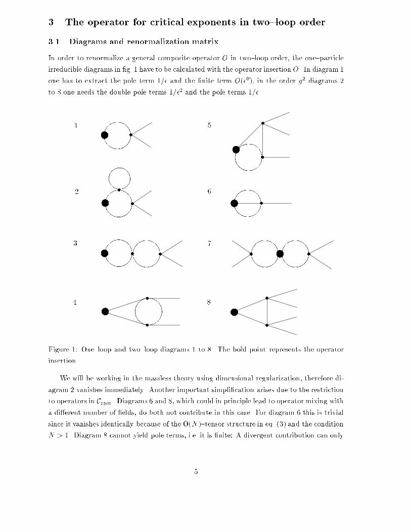
3.1 Diagrams and renormalization matrix
In order to renormalize a general composite operator O in two{loop order, the one{particle
irreducible diagrams in �g. 1 have to be calculated with the operator insertion O. In diagram 1
one has to extract the pole term 1=� and the �nite term O(�
0
), in the order g
2
diagrams 2
to 8 one needs the double pole terms 1=�
2
and the pole terms 1=�.
&%
'$
&%
'$
&%
'$
&%
'$
w
&%
'$
&%
'$
w
&%
'$
w
&%
'$
&%
'$
z
z
z
z
z
z
1
2
3
4
5
6
7
z
��
��
8
z
s
s
s
s
s
s
s
s
s
s
ss
s
s
Figure 1: One{loop and two{loop diagrams 1 to 8. The bold point represents the operator
insertion.
We will be working in the massless theory using dimensional regularization, therefore di-
agram 2 vanishes immediately. Another important simpli�cation arises due to the restriction
to operators in C
sym
. Diagrams 6 and 8, which could in principle lead to operator mixing with
a di�erent number of �elds, do both not contribute in this case. For diagram 6 this is trivial
since it vanishes identically because of the O(N){tensor structure in eq. (3) and the condition
N > 1. Diagram 8 cannot yield pole terms, i.e. it is �nite: A divergent contribution can only
5

w
�
�
�
�1
P
P
P
Pq
}
�
�
�
�:
.
.
.
O
p =)
p
1
p
2
p
n
ext
Diagrams
1 to 8
Figure 2: Composite operator insertion in a vertex function with n
ext
external legs.
occur if internal momenta generated by gradients in the composite operator cancel one of the
propagators in the denominator. Since operators in C
sym
are traceless in the spatial indices,
this cannot happen here.
We are left with the calculation of diagrams 1,3,4,5 and 7 for a general operator insertion
from C
sym
. The details of this lengthy calculation can be found in the appendix. The main
problem is to �nd expressions for the coe�cients multiplying the pole terms which exhibit
the dependence on the operator insertion in a simple manner.
The pole terms determine the renormalization factors of the composite operators in a
standard way. Renormalized and bare vertex functions are connected via the renormalization
matrix Z
A
k
A
j
�
R
A
k
(p
1
; . . . ; p
n
ext
; p)Z
A
k
A
j
Z
�n
ext
=2
�
= �
B
A
j
(p
1
; . . . ; p
n
ext
; p): (15)
Here �
R
A
k
denotes the renormalized vertex function with operator insertion A
k
, similarly
�
B
A
j
for the bare vertex function. n
ext
is the number of external legs, p
1
; . . . ; p
n
ext
are the
associated external momenta and p is the momentum of the operator insertion, compare
�g. 2. Z
�
in eq. (15) is the wave{function renormalization factor [23]
Z
�
= 1�
~
g
2
�
N + 2
144
+O(~g
3
): (16)
The renormalization factor in eq. (15) expressed in terms of creation and annihilation oper-
ators follows from the Feynman diagrams calculated in appendix A
Z Z
�n
ext
=2
�
= 1 + ~gX + ~g
2
Y +O(~g
3
)
) Z = 1 + ~gX + ~g
2
Y �
n
ext
2
~g
2
�
N + 2
144
+O(~g
3
) (17)
with
X = �
1
6
1
X
l=0
l
X
k;j=0
1
l + 1
a
y
j
a
y
l�j
a
k
a
l�k
(18)
�
�
1
�
+
1
2
ln
�
2
(p
j
+ p
l�j
)
2
�
1
2
+ (S
l+1
�
1
2
S
k
�
1
2
S
l�k
) +O(�)
�
6

from eq. (78). S
j
is the sum
S
j
=
j
X
k=1
1
k
: (19)
The lengthy expression for Y is the sum of the contributions in order ~g
2
and can be found in
the appendix, eq. (79). Z
A
k
A
j
is now equivalent to the matrix element < A
k
jZjA
j
> in this
creation/annihilation language.
In eq. (18) p
j
denotes the momentum of the �eld generated by a
y
j
. Similar logarithms
of momenta can also be found in the expression for Y . However, one can get rid of these
logarithms by a suitable subtraction scheme. Instead of the renormalization factor in eq. (17)
we use the equivalent factor
Z = (1� ~gX
fin
)
�
1 + ~gX + ~g
2
Y �
n
ext
2
~g
2
�
N + 2
144
�
+ O(~g
3
)
= 1 + ~gX
pole
+ ~g
2
(Y �X
fin
X
pole
)�
n
ext
2
~g
2
�
N + 2
144
+O(~g
3
): (20)
Here X
fin
is the �nite part of X from eq. (18) and X
pole
the pole term
X
pole
= �
1
6�
1
X
l=0
1
l+ 1
l
X
k;j=0
a
y
j
a
y
l�j
a
k
a
l�k
(21)
X
fin
= X �X
pole
: (22)
One can check in a straightforward calculation that all renormalization scale dependent log-
arithms in the combination Y �X
fin
X
pole
cancel.
3.2 The two{loop mixing matrix in C
sym
The mixing matrix (more precisely: mixing operator) follows in the usual manner from the
renormalization matrix
M =
�
N
d
�(~g)
d
d~g
Z
�
Z
�1
: (23)
With the �{function [23]
N
d
�(~g) = �� ~g +
N + 8
6
~g
2
+ O(~g
3
) (24)
this is
M
(2lp)
=
n
2
~g
2
N + 2
72
� � ~gX
pole
+ � ~g
2
X
2
pole
+ ~g
2
N + 8
6
X
pole
�2� ~g
2
(Y �X
fin
X
pole
) + O(~g
3
); (25)
where we have made use of the fact that in all vertex functions contributing here the numer
of external �elds is equal to the number of �elds in the composite operator n
ext
= n. All
7

double pole terms in (25) cancel as they should do. By combining the appropriate terms one
�nally �nds after some lengthy but simple algebra
M
(2lp)
=
n
2
� + ~g
c
V
(1lp)
+ ~g
2
c
�
V
(2lp)
2
+ V
(2lp)
3
�
+O(�
3
) (26)
at the critical point [23]
~g
c
= �
6
N + 8
+ �
2
18(3N + 14)
(N + 8)
3
+O(�
3
): (27)
� follows from wave{function renormalization
� = �
2
N + 2
2(N + 8)
2
+ O(�
3
): (28)
In eq. (26) V
(1lp)
is the already known one{loop term eq. (8)
V
(1lp)
=
1
6
1
X
l=0
1
l+ 1
l
X
k;j=0
a
y
j
a
y
l�j
a
k
a
l�k
: (29)
The two{loop terms can be split up in a two{particle interaction operator
V
(2lp)
2
= �
N + 6
36
1
X
l=0
l
X
k;j=0
1
l+ 1
�
h
1�
1
2(l+ 1)
+
1
2
I(k < j)(S
k
� S
j
) +
1
2
I(k > j)(S
l�k
� S
l�j
)
i
� a
y
j
a
y
l�j
a
k
a
l�k
(30)
with
I(true) = 1; I(false) = 0 (31)
and the three{particle interaction part given by
V
(2lp)
3
= �
1
9
1
X
l=0
l
X
k
1
;j
1
=0
l�k
1
X
k
2
=0
l�j
1
X
j
2
=0
1
j
1
+ j
2
+ 1
1
k
1
+ k
2
+ 1
�
h
1
2
(S
l�k
1
�k
2
� S
l+1
)
+(S
k
1
+k
2
+1
�
1
2
S
k
1
�
1
2
S
k
2
) I(k
1
+ k
2
+ j
1
+ j
2
� l)
+
1
2
(S
l�j
1
�j
2
� S
l�k
1
�k
2
�j
1
�j
2
�1
) I(k
1
+ k
2
+ j
1
+ j
2
< l)
i
� a
y
j
1
a
y
j
2
a
y
l�j
1
�j
2
a
k
1
a
k
2
a
l�k
1
�k
2
: (32)
Notice that possible four{particle interaction terms have cancelled in eq. (25).
Eq. (26) is the key computational result of this paper. A right eigenvector j(c)> ofM
(2lp)
with n �elds and l gradients
M
(2lp)
j(c)>= � j(c)> (33)
8

corresponds to a two{loop eigenoperatorO(t;h; c) of the renormalization ow with anomalous
dimension � as explained in sect. 2. Its critical exponent is
x = n
�
1�
�
2
�
+ l + �+O(�
3
): (34)
One can introduce an operator of critical exponents X to code (34) into a compact expression
X =
�
1�
�
2
+
�
2
�
^
N +
^
L+ ~g V
(1lp)
+ ~g
2
�
V
(2lp)
2
+ V
(2lp)
3
�
(35)
to be evaluated at the critical point ~g = ~g
c
. Here
^
N gives the number of �elds
^
N =
1
X
l=0
a
y
l
a
l
(36)
and
^
L the number of gradients
^
L =
1
X
l=0
l a
y
l
a
l
: (37)
4 Eigenoperators and critical exponents
4.1 General properties of the operator of critical exponents
The operator X in eq. (35) encodes the complete two{loop spectrum of critical exponents and
the corresponding eigenoperators in C
sym
. In this sense it gives the solution of the universal
properties of the N{vector model in this subspace in two{loop order. Before we go on to
obtain explicit information about the spectrum, let us establish some general properties of X .
First of all, M
(2lp)
commutes with the operators S and the derivative operator D from
eq. (12). The commutator with S is trivial and the commutator withD follows from unbroken
translation invariance (it can also be checked in a lengthy calculation). Hence
[S;X ] = 0
[D;X ] = �D: (38)
In one{loop order the commutator [D; V
(1lp)
] = 0 immediately implied the existence of an-
other symmetry operator D
y
since V
(1lp)
is hermitean. In two{loop order this simple argu-
ment no longer holds sinceM
(2lp)
is not hermitean: Both V
(2lp)
2
and V
(2lp)
3
are non{hermitean.
Therefore the naive/canonical representation of the conformal group induced by D;D
y
and S
is no longer a symmetry group on the operator algebra beyond one{loop order.
However, it can be shown [19] that it is possible to modify the canonical representation
by terms in order � yielding the explicit representation of the conformal symmetry group
on C
sym
in two{loop order. For the purpose of this paper it will be su�cient to argue that
one only needs to �nd the non{derivative eigenoperators of X that due to eq. (38) generate
the whole spectrum.
9

Another property that cannot be extended beyond one{loop order is the lower bound zero
for the anomalous dimensions [6] following from
V
(1lp)
� 0: (39)
E.g. operators without gradients with n �elds
t
i
1
...i
n
�
i
1
� . . . � �
i
n
; t
i
1
...i
n
symmetric and traceless (40)
are easily seen to be eigenoperators of X with critical exponent
x =
�
1�
�
2
+ �
2
N + 2
4(N + 8)
2
�
n+
�
�
N + 8
� �
2
N
2
� 4N � 36
2(N + 8)
3
�
n(n� 1)
��
2
2
(N + 8)
2
n(n � 1)(n� 2) +O(�
3
) (41)
in agreement with former results [5]. For a �xed positive � this exponent can become arbi-
trarily negative for a large number of �elds since the term proportional to n
3
comes with a
minus sign. However, this implies no danger for the stability of the nontrivial �xed point
since the term proportional to n
4
in order �
3
is known to give a positive contribution [18]. It
is after all not surprising that the asymptotic �{expansion generates terms with alternating
signs in di�erent orders.
In contrast for the 2 + �{expansion in the N{vector model the situation is more worri-
some. Both one{loop [20] and two{loop calculations [2] make a class of operators with many
gradients more and more relevant for a given positive �. This stability problem for the non-
trivial �xed point in the 2 + � expansion remains so far unresolved and seems to be generic
for 2 + � expansions in all models [9, 10, 21, 14].
4.2 Results for two �elds
For composite operators with n = 2 �elds and l gradients the critical exponents have already
been calculated in the pioneering work of Wilson [22] up to order �
2
. These results are
rederived here in our formalism as a consistency check. In addition we also obtain the
explicit structure of the eigenoperators that cannot be found in the calculational scheme of
ref. [22].
O(N) symmetric and traceless tensors:
Non{derivative composite operators only exist for an even number of gradients l. Diagonal-
ization of X yields:
� l = 0 : Eigenoperator t
i
1
i
2
�
i
1
�
i
2
, t
i
1
i
2
symmetric and traceless, with critical exponent
x = 2� �
N + 6
N + 8
� �
2
N
2
� 18N � 88
2(N + 8)
3
+ O(�
3
): (42)
10

� l = 2; 4; . . . : Eigenoperator t
i
1
i
2
h
�
1
...�
l
T
�
1
...�
l
i
1
i
2
, t
i
1
i
2
and h
�
1
...�
l
symmetric and traceless,
where
T
�
1
...�
l
i
1
i
2
=
l
X
k=0
(�1)
k
�
l
k
�
2
@
�
1
. . .@
�
k
�
i
1
@
�
k+1
. . .@
�
l
�
i
2
�~g
N + 6
6
1
l(l+ 1)
@
�
1
. . .@
�
l
(�
i
1
�
i
2
)
+~g
l�2
X
p=2
even
c
l;p
@
�
p+1
. . .@
�
l
T
�
1
...�
p
i
1
i
2
+O(~g
2
): (43)
with critical exponent
x = 2
�
1�
�
2
+
�
2
�
+ l � �
2
N + 6
(N + 8)
2
1
l(l+ 1)
+O(�
3
): (44)
The coe�cients c
l;p
in the eigenoperators with l = 4; 6; . . . are arbitrary. They result
from the one{loop degeneracy of the anomalous dimensions for l = 2; 4; . . . and can only
be �xed in a three{loop calculation.
The one{loop degeneracies in the spectrum are completely lifted by the terms in order �
2
in
eq. (44) as already known from ref. [22]. A characteristic new feature is the spatial derivative
of �
i
1
�
i
2
in the eigenoperator in order ~g. Hence the eigenoperators are not invariant with
respect to D
y
from eq. (12)
D
y
T
�
1
...�
l
i
1
i
2
(0) 6= 0; (45)
that is they are not canonically conformal invariant operators. We come back to this point
in sect. 6.
O(N) scalar tensors:
Since diagram 6 does not contribute for n = 2, one can also deal with O(N) scalar tensors in
this special case by using the appropriate combinatorial factors for the other diagrams. The
operator of critical exponents on this subspace is
X
�
�
�
n=2
= 2
�
1�
�
2
+
�
2
�
+ l + ~g
N + 2
12
1
X
l=0
1
l+ 1
l
X
j;k=0
a
y
j
a
y
l�j
a
k
a
l�k
�~g
2
N + 2
12
1
X
l=0
l
X
k;j=0
1
l+ 1
a
y
j
a
y
l�j
a
k
a
l�k
(46)
�
h
1�
1
2(l+ 1)
+
1
2
I(k < j)(S
k
� S
j
) +
1
2
I(k > j)(S
l�k
� S
l�j
)
i
Like for the O(N) symmetric and traceless case one derives:
11

� l = 0 : Eigenoperator
~
�
2
with critical exponent
x = 2� �
6
N + 8
+ �
2
(N + 2)(13N + 44)
2(N + 8)
3
+ O(�
3
): (47)
� l = 2; 4; . . . : Eigenoperator h
�
1
...�
l
�
T
�
1
...�
l
, h
�
1
...�
l
symmetric and traceless, where
�
T
�
1
...�
l
=
l
X
k=0
(�1)
k
�
l
k
�
2
(@
�
1
. . .@
�
k
~
�) � (@
�
k+1
. . .@
�
l
~
�)
�~g
1
l(l+ 1)
@
�
1
. . .@
�
l
~
�
2
+~g
l�2
X
p=2
even
�c
l;p
@
�
p+1
. . .@
�
l
�
T
�
1
...�
p
+O(~g
2
): (48)
with critical exponent
x = 2
�
1�
�
2
+
�
2
�
+ l � �
2
N + 2
2(N + 8)
2
6
l(l+ 1)
+O(�
3
): (49)
The same remarks as for the O(N) symmetric and traceless tensors hold here too. In
particular the critical exponents are consistent with ref. [22].
The special case with l = 2 gradients deserves some attention. In this case the critical
exponent equals the dimension of space
x = d (50)
and the corresponding scaling eigenoperator is proportional to the stress tensor
�
(m
1
;m
2
)
= h
(m
1
;m
2
)
��
�
@
�
~
� � @
�
~
��
�
1
6
�
~g
36
�
@
�
@
�
~
�
2
�
+O(~g
2
) (51)
as it should be. The magnetic quantum numbers m
1;2
= �1=2 label the symmetric and trace-
less tensors h
(m
1
;m
2
)
��
and correspond to the two SO(3) sectors of the rotation group SO(4).
The renormalized stress tensor follows via the renormalization matrix Z and one can show
after a short calculation
�
R (m
1
;m
2
)
= h
(m
1
;m
2
)
��
�
@
�
~
� � @
�
~
��
�
1
6
�
~g
36
�
1 +
~g
�
N + 2
12
�
�
@
�
@
�
~
�
2
�
+O(~g
2
�
0
) +O(~g
3
): (52)
This is consistent with the alternative de�nition of the renormalized stress tensor to be the
response of the renormalized action in curved space with respect to a variation of the metric
(for the two{loop renormalized action of scalar �
4
{theory in curved space compare ref. [13]).
12

4.3 More complicated composite operators
It is not very illuminating to write down a complete list of eigenvalues of the operator of
critical exponents for n > 2. All this information is contained in our operator X anyway. We
will only concentrate on some important features of the two{loop spectrum.
Comparison with 1=N{expansions:
The nonlinear �{model describes the second order phase transition in the universality class
of the N{vector model coming from the ordered low{temperature phase. The (
~
�
2
)
2
{theory
describes this transition coming from the high{temperature phase. Critical exponents of
observables should therefore be consistent in the 1=N{expansion in the nonlinear �{model
and the 4� � expansion here. This idea has e.g. been successfully tested for the elementary
�eld and the energy density in refs. [16, 17]. Since Lang and R�uhl have derived a scheme
to obtain critical exponents for composite operators in the 1=N{expansion in the nonlinear
�{model for 2 < d < 4 dimensions [12], it requires little extra work to check consistency
also for more complicated composite operators. Besides this o�ers a valuable test for the
correctness of the lengthy calculations in both approaches.
Tables 1 and 2 contain the critical exponents for the �rst non{derivative eigenoperators
with n = 3 and n = 4 �elds. We use the notation
x = n
�
1�
�
2
+
�
2
�
+ l+ ~g
c
�
(1lp)
+ ~g
2
c
�
N + 6
36
�
(2lp)
2
+
1
9
�
(2lp)
3
�
+ O(�
3
) (53)
where the coe�cients �
(1lp)
; �
(2lp)
2
and �
(2lp)
3
follow from V
(1lp)
; V
(2lp)
2
and the three particle
interaction V
(2lp)
3
, resp.
Gradients �
(1lp)
�
(2lp)
2
�
(2lp)
3
l = 0 1 �3 �3
l = 2 5=9 �16=9 �7=54
l = 3 1=6 �13=12 �5=96
l = 4 7=15 �203=150 61=1500
l = 5 2=9 �391=360 �91=1080
l = 6 3=7 �5189=4410 541=6860
0 �5=18 0
Table 1: Non{derivative eigenoperators with n = 3 �elds and l � 6 gradients. The critical
exponents follows with eq. (53).
In the 1=N{expansion Lang and R�uhl obtained the critical exponents of composite op-
erators with transformation properties (2) as continuous functions of the space dimension d
13

Gradients �
(1lp)
�
(2lp)
2
�
(2lp)
3
l = 0 2 �6 �12
l = 2 13=9 �79=18 �265=54
l = 3 1 �7=2 �5=2
Table 2: Non{derivative eigenoperators with n = 4 �elds and l � 3 gradients.
for 2 < d < 4. One can expand these exponents to second order in � for d = 4 � � and
compare the resulting coe�cients with the coe�cients in order N
0
and 1=N in eq. (53). We
found perfect agreement of �
(1lp)
and �
(2lp)
2
for all composite operators contained in tables 1
and 2.
2
The coe�cient �
(2lp)
3
only contributes in order 1=N
2
and cannot be compared there-
fore. The agreement of factors like �
5189
4410
�
2
N
gives good enough reason to expect consistency
for general l; n.
Resolution of degeneracies with eigenvalue zero:
A surprising result in one{loop order are the degeneracies of eigenoperators with vanishing
anomalous dimensions [7]. For two �elds it was already well known that these degeneracies
are lifted in order �
2
(compare sect. 4.2). In general we will �nd the same resolution for
n > 2 �elds.
Tables 3 and 4 collect the �rst critical exponents for non{derivative eigenoperators with
�
(1lp)
= 0. One can easily establish
V
(1lp)
j>= 0 ) < jV
(2lp)
3
j>= 0 (54)
by using the structure of the eigenoperators with one{loop eigenvalue zero as found in closed
form in ref. [7]. Hence �
(2lp)
3
= 0 and only �
(2lp)
2
is tabulated.
Except for the case n = 3 with l = 6 or l = 8 gradients all one{loop degeneracies are
resolved. In fact this resolution of degeneracies holds as far as we have tested it on a computer
(up to at least l = 22 for arbitrary n).
Resolution of degeneracies with nonzero eigenvalues:
We observed another class of generic degeneracies for n = 4 �elds and an odd number of
gradients in ref. [7]. The complete solution for this part of the spectrum was recently given
by Derkachov and Manashov in ref. [3]. In two{loop order we again notice from table 5 that
the degeneracies are lifted. This also holds as far as we have tested it (up to at least l = 22).
2
I thank K. Lang for making the explicit values of the 1=N{coe�cients based on the works cited in ref. [12]
available to me.
14

Gradients �
(2lp)
2
l = 6 �5=18
l = 8 �5=18
�
still degenerate
l = 9 �79=672
l = 10 �23=84
l = 11 �2599=21600
l = 12 �0:268 . . .
�0:0642 . . .
Table 3: The �rst non{derivative eigenoperators with n = 3 �elds and vanishing one{loop
eigenvalue �
(1lp)
= 0 () �
(2lp)
3
= 0).
Gradients �
(2lp)
2
l = 12 �251=675
l = 14 �731=1944
l = 15 �5897=16200
l = 16 �0:379 . . .
�0:188 . . .
Table 4: The �rst non{derivative eigenoperators with n = 4 �elds and vanishing one{loop
eigenvalue �
(1lp)
= 0 () �
(2lp)
3
= 0).
Gradients �
(1lp)
�
(2lp)
2
�
(2lp)
3
l = 3 1 �7=2 �5=2
l = 5 1 �199=60 �161=60
l = 7 1 �451=140 �389=140
1=3 �109=60 3=20
l = 9 1 �5317=1680 �4763=1680
1=3 �477=280 11=105
5=9 �8249=5040 �1109=15120
Table 5: Non{derivative eigenoperators with n = 4 �elds and an odd number of gradients
l � 9.
15

5 A conjecture about the structure of the spectrum
Let us put the information about the spectrum of anomalous dimensions together that we
have obtained here and in refs. [6, 7]. Its graphical representation in �g. 3 leads to the
following conjecture:
Let �
1
be the anomalous dimension of a non{derivative eigenoperator with
n
1
�elds, �
2
likewise for an eigenoperator with n
2
�elds. Then � = �
1
+ �
2
is a limit point in the spectrum of anomalous dimensions with n
1
+ n
2
�elds.
A similar conjecture has been formulated independently by Derkachov and Manashov in
ref. [3].
3
We will later see how this gives rise to a remarkable in�nite hierarchical structure
of the spectrum.
The intuitive idea behind the conjecture follows an idea due to Parisi [1]. He argued that
for composite operators like � @
�
1
. . .@
�
l
� in the limit of large spin l ! 1, no further sub-
tractions are necessary besides the wave function renormalization of the elementary �elds �.
Intuitively a large angular momentum \e�ectively" separates two space points. It seems to
be possible to generalize this conjecture in the following manner: Let O
1
(O
2
) be a non{
derivative eigenoperator from C
sym
with anomalous dimension �
1
(�
2
) consisting of n
1
(n
2
)
�elds and l
1
(l
2
) gradients. Consider the composite operator made up of O
1
and O
2
P
l
[O
1
; O
2
] =
l
X
k=0
m
l
k
(D
k
O
1
) (D
l�k
O
2
) (55)
with coe�cients m
l
k
chosen as to make P
l
[O
1
; O
2
] canonically conformal invariant
m
l
k
= (�1)
k
�
l
k
�
1
(k � 1 + 2l
1
+ n
1
)! (l� k � 1 + 2l
2
+ n
2
)!
: (56)
For �nite l, P
l
[O
1
; O
2
] will generally not be an eigenoperator. But for l!1 it approximates
better and better a one{loop eigenoperator with an anomalous dimension � given by the
naive sum of �
1
and �
2
� = �
1
+ �
2
: (57)
In this sense the derivatives D in eq. (55) \divide" the two parts of the composite opera-
tor P
l
[O
1
; O
2
].
Though a closed proof of the above statement cannot be given, numerical calculations
with eq. (55) strongly support these intuitive ideas for general n in one{loop order. It is easy
to check this and we will refrain from giving a lengthy list of explicit examples. One problem
in the proof is the existence of the composite operators P
l
[O
1
; O
2
], since the sum in eq. (55)
3
I thank the authors for informing me of their work prior to publication.
16

6
�� n
�
2
h
�
6
N+8
i
0
1
n = 1
�
i
1
n = 2
�
i
1
�
i
2
(
l=1
l=2
.
.
.
T
�
1
...�
l
i
1
i
2
n = 3
�
i
1
�
i
2
�
i
3
P
1
[�
i
1
�
i
2
; �
i
3
]
(
n = 4
�
i
1
�
i
2
�
i
3
�
i
4
P
1
[�
i
1
�
i
2
; �
i
3
�
i
4
]
(
Figure 3: Anomalous dimensions � with wave function renormalization subtracted for non{
derivative eigenoperators from C
sym
, eq. (2) with n = 1 to n = 4 �elds. Full lines denote
discrete eigenvalues, dashed lines are limit points in the spectrum. The linethickness of the
dashed lines indicates the hierarchy of limit points. O(�
2
){splittings are qualitatively depicted
with the brackets (only shown for the smallest eigenvalues). n = 4 also includes results from
ref. [3]. For further explanations see text.
can vanish for particular values of l. In two{loop order things are more complicated since in
general the coe�cients m
l
k
are modi�ed by terms in order � making numerical calculations
more involved. Still the results are in very good agreement with the conjecture.
It is interesting to notice that a similar structure of \limit points" can also be found in
1=N{expansions: Since anomalous dimensions depend continuously on d in 1=N{expansions,
it is more precise to speak of limit curves then. These have been observed for various classes
of composite operators in ref. [11]. Hence one might expect that the conjecture holds to all
orders in the 4� � expansion.
Let us be more explicit by looking at composite operators with n = 1 to n = 4 �elds
from C
sym
, where the above ideas can in some cases be shown exactly. The anomalous
dimensions � of these non{derivative operators are plotted in �g. 3. For convenience the
contribution n �=2 coming from wave function renormalization has been subtracted every-
17

where. In general only the order � part of the anomalous dimension is depicted, except for
the lowest{lying eigenvalues where a qualitative impression of the order �
2
{splittings is given
by the brackets. If one neglects these two{loop e�ects, �g. 3 is also the spectrum of anomalous
dimensions in scalar �
4
{theory in units of [�].
� n = 2 : Going from left to right in the �gure, the anomalous dimension of the elementary
�elds goes over in the family T
�
1
...�
l
i
1
i
2
for n = 2. According to the conjecture � = 2�
�
i
= �
appears as a limit point there indicated by the dashed line. It is approached by the
discrete eigenvalues belonging to the eigenoperators T
�
1
...�
l
i
1
i
2
from eq. (44). One other
eigenvalue belonging to �
i
1
�
i
2
appears.
� n = 3 : In agreement with the conjecture, there is the limit point P
1
[�
i
1
�
i
2
; �
i
3
] for three
�elds. In �g. 3 this is the dashed line with � = �
2
N+8
+O(�
2
). The discrete eigenvalues
approaching it have already been worked out in ref. [6] in closed form. Close to the
limit point the eigenvalues lie very densely and are indicated by the hatched areas.
Furthermore each of the formerly discrete eigenvalues belonging to T
�
1
...�
l
i
1
i
2
can be com-
bined with an elementary �eld and becomes a limit point. The discrete eigenvalues
approaching these limit points are not shown. In this manner a limit point of limit
points is generated for � = 3
�
2
and depicted by the thicker dashed line.
� n = 4 : Only the largest of the discrete eigenvalues belonging to �
i
1
�
i
2
�
i
3
�
i
4
is shown
here. In addition it has already been observed in ref. [7] that the discrete eigenvalues for
three �elds appear here again with in�nite multiplicities. Derkachov and Manashov have
given a proof for this [3] and in addition shown that there is another limit point with � =
�
4
N+8
+ O(�
2
). According to the conjecture this can be identi�ed as P
1
[�
i
1
�
i
2
; �
i
3
�
i
4
]
in �g. 3. The other limit points with � > O(�
2
) obviously come from the combination
of an elementary �eld with an eigenoperator with three �elds.
Order �
2
{corrections resolve the in�nite multiplicities and turn them into true limit
points: If one does the two{loop calculation for su�ciently large l, one �nds good
evidence that eq. (57) holds in two{loop order too. Hence the former P
1
[�
i
1
; �
i
2
�
i
3
]
turns into a limit point of limit points here. Similarly for � = 2� one now �nds a limit
point of limit points of limit points.
It should be remarked that the above remarks have been proven in order � in refs. [6, 7, 3].
In order �
2
and for n = 3; 4 the numerical evidence based on explicit diagonalizations is very
good for non{degenerate subspaces. For subspaces that are degenerate in one{loop order,
e.g. the lowest{lying eigenvalues, the approach to the limit points is slow (though steady)
and an analytic proof would be desirable. In any case for a general number of �elds some
di�erent technique will be necessary to prove the conjecture.
18

Summing up, one would propose that for an increasing number of �elds n, higher and
higher hierarchies of limit points are generated by the rules
sum of two discrete eigenvalues �! limit point
sum of a discrete eigenvalue and a limit point �! limit point of limit points
and so on. This produces an interesting in�nite hierarchical structure in the spectrum of
anomalous dimensions. For n!1 the spectrum might even have fractal properties.
6 Conformal covariance in real space
6.1 Two{point correlation functions of composite operators
So far we have mainly been concerned with the spectrum of anomalous dimensions. In this
section follows a short aside discussing the structure of the respective eigenoperators. The
generic new feature in two{loop order are \anomalous" (i.e. order �) terms in the eigenoper-
ators, compare for example eqs. (43) or (48). We want to demonstrate how this is connected
with the idea of conformal symmetry, which is expected at the critical point of the N{vector
model, thereby going beyond the well{established concept of global scale invariance. The
most complete and rigorous treatment of this point is due to Sch�afer [15].
4
One important consequence of conformal invariance is that two non{derivative eigenoper-
ators with di�erent critical exponents are uncorrelated in a two{point function at the critical
point
x
A
1
6= x
A
2
) < A
R
1
(r
1
)A
R
2
(r
2
)>
c
= 0: (58)
Here A
R
i
are the renormalized eigenoperators. In principle the theorem (58) was already
stated by Ferrara, Gatto and Grillo [4], but only in ref. [15] it became clear why the re-
striction to non{derivative eigenoperators is necessary. Of course all total spatial derivatives
of A
1
and A
2
are also uncorrelated after x
A
1
6= x
A
2
has been shown for the non{derivative
eigenoperators.
The terms in order � in the two{loop eigenoperators will now turn out to be exactly the
necessary correction terms to make eq. (58) hold to order �. In fact one can use eq. (58) as an
alternative starting point to calculate these anomalous terms. It should be noted that such
terms in the eigenoperators are no more \anomalous" than the anomalous dimension in the
4
In fact Sch�afer establishes some conditions under which global scale invariance implies local scale invariance
(i.e. conformal invariance). To the best of our knowledge there is no proof in the literature that all these
conditions are actually ful�lled in the N{vector model, in particular his condition (Kii) regarding possible
surface terms. Still we consider it plausible.
19

critical exponent. With respect to special conformal transformations they play a similar role
like anomalous dimensions with respect to dilatations.
Let us make these points more explicit. We will calculate the two{point correlation
function for composite operators up to terms in order �. For the purpose of this section it
will prove to be su�cient to consider operators from C
sym
that couple to maximum spin. One
can achieve this by doing the calculation for composite operators A
1
; A
2
with structure (68)
A
1;2
= t
(1;2)
i
1
...i
n
1;2
�
�
1
. . .�
�
l
1;2
A
i
1
...i
n
1;2
�
1
...�
l
1;2
(c
(1;2)
); (59)
A
i
1
...i
n
1;2
�
1
...�
l
1;2
(c
(1;2)
) like in eq. (4) and � = (i=2; 0; 0; 1=2).
It is easy to see that up to order g, non{vanishing contributions in the two{point func-
tion (58) of O(N){traceless tensors can only arise for the same number n of �elds in both
A
1
and A
2
. Details of the calculation of the two{point correlation function for renormalized
eigenoperators are worked out in appendix B. The result is
< A
R
1
(r
1
)A
R
2
(r
2
)>
c
=
2
l
1
+l
2
+2n(1��=2)
(4�)
nd=2
(� � r)
l
1
(�� � r)
l
2
(r
2
)
l
1
+l
2
+n(1��=2)
�
��
1� ~g
�
�
A
1
~g
c
+
�
A
2
~g
c
�
�
ln(� r)� ln 2�
1
2
(2)
�
�
A
(0)
0
+
�
� + ~g
�
�
A
1
~g
c
+
�
A
2
~g
c
��
A
(0)
�
�
4
3
~g A
(1)
�
�
+~g O(�) + O(~g
2
) (60)
with r = r
2
�r
1
. �
A
1
; �
A
2
are the anomalous dimensions of A
1
; A
2
, resp., and the amplitudes
A
(0)
0
, A
(0)
�
, A
(1)
�
can be found in appendix B. The correct scaling behaviour follows as usual
by exponentiating logarithms.
6.2 Composite operators with two �elds
O(N) symmetric and traceless tensors:
Consider the operator S
l
= t
(1)
i
1
i
2
�
�
1
. . .�
�
l
S
�
1
...�
l
i
1
i
2
for even l with
S
�
1
...�
l
i
1
i
2
=
l
X
k=0
(�1)
k
�
l
k
�
2
@
�
1
. . .@
�
k
�
i
1
@
�
k+1
. . .@
�
l
�
i
2
+ ~g c
l;0
@
�
1
. . .@
�
l
(�
i
1
�
i
2
) (61)
where c
l;0
is some arbitrary coe�cient. S
l
is a one{loop eigenoperator for arbitrary c
l;0
, but
in two{loop order the correct scaling behaviour requires according to eq. (43)
c
l;0
= �
N + 6
6
1
l(l+ 1)
: (62)
Alternatively conformal covariance says
<
�
S
l
�
R
(0)
�
t
(2)
i
1
i
2
�
i
1
�
i
2
�
R
(r)>
c
!
= 0: (63)
20

From eq. (60) one �nds after some calculation
<
�
S
l
�
R
(0)
�
t
(2)
i
1
i
2
�
i
1
�
i
2
�
R
(r)>
c
=
X
i
1
;i
2
t
(1)
i
1
i
2
t
(2)
i
1
i
2
�
�
2�
l
� ~g
2
3l
+ ~g c
l;0
2(l+ 1)
�
+~g O(�) + O(~g
2
)
!
= 0; (64)
therefore
~g c
l;0
=
1
l(l+ 1)
�
~g
3
� �
�
(65)
in agreement with eq. (62) at the critical point.
The anomalous terms in the two{loop eigenoperators can in this manner be derived from
an order g calculation: The coupling to the spatial derivative of �
i
1
�
i
2
in the eigenoperator
can be uniquely �xed by requiring that the eigenoperator is uncorrelated with �
i
1
�
i
2
, eq. (63).
In a similar manner one could derive all the other anomalous terms c
l;p
in eq. (43) by requiring
< S
R
l
(0) S
R
p
(0)>
c
= 0: (66)
O(N) scalar tensors:
For O(N) scalar tensors with two �elds we have also been able to �nd the scaling eigenop-
erators in sect. 4.2. Besides di�ering combinatorial factors, the calculation of the two{point
function runs along the same lines as in appendix B. Again one can see explicitly that eq. (58)
holds for all correlation functions of the operators
�
T
�
1
...�
l
from eq. (48) with
~
�
2
. In particular
this is true for the correlation function of stress tensor (52) and energy density
< �
R (m
1
;m
2
)
(r
1
)
�
~
�
2
�
R
(r
2
)>
c
= 0 +O(�
2
): (67)
This property holds only for the coe�cient of the improvement term @
�
@
�
~
�
2
in the stress
tensor that we have found in sect. 4.2.
6.3 More complicated composite operators
So far we have looked at correlation functions of non{derivative operators where already the
canonical critical exponents were di�erent. A new feature arises for n > 2 �elds since then
one can have linearly independent non{derivative operators with the same number of �elds
and gradients. In this case the critical exponents in eq. (58) only di�er by terms in order �
or higher.
Due to the generally very complicated structure of the two{loop eigenoperators for n > 2,
we cannot give closed formulas here. However, we have checked explicitly that the two{
point correlation functions of all the composite operators in tables 1 to 5 with each other are
consistent with theorem (58).
21

7 Conclusions
The spectrum of anomalous dimensions in the operator subalgebra C
sym
of the N{vector
model has been investigated to order �
2
in the d = 4 � � expansion. This analysis became
possible using the concept of a spectrum{generating operator introduced in ref. [6]. The
complete spectrum is encoded in the spectrum{generating operator and it is straightforward
to extract anomalous dimensions and the corresponding eigenoperators.
An interesting consistency check in its own right is provided by comparison of critical
exponents in the �{expansion here with results from 1=N{expansions in the nonlinear �{
model for 2 < d < 4 dimensions by Lang and R�uhl [12]. Due to the resolution of one{loop
degeneracies in two{loop order, we make the same observation as in the 1=N{expansion
that generically quasiprimary operators (non{derivative eigenoperators) generate indepen-
dent conformal blocks. Another consistency check sensitive to the structure of the eigenop-
erators was provided by testing conformal covariance of two{point correlation functions of
composite operators in sect. 6. Anomalous terms in the eigenoperators are found to play a
similar role with respect to special conformal transformations as anomalous dimensions with
respect to dilatations.
A key observation in this work is the in�nite hierarchical structure in the spectrum as
depicted in �g. 3. Such a structure follows naturally from the conjecture that for any two
eigenoperators O
1
; O
2
, one can construct approximate eigenoperators P
l
[O
1
; O
2
] as in eq. (55)
that become exact eigenoperators in the limit l!1. The anomalous dimension is then just
given by the naive sum of the two constituent anomalous dimensions. The intuitive idea
behind this conjecture is that the two constituents O
1
; O
2
become \separated" for large l.
These ideas have been numerically and analytically well{supported, though a general proof
is still an open problem. A similar conjecture was formulated independently by Derkachov
and Manashov [3].
Thus the spectrum of this well{investigated d dimensional �eld theory seems to possess
a fascinating in�nite hierarchical structure of limit points that allows for fractal properties
in the limit of a large number of �elds n ! 1. It is an interesting question whether such
properties of spectra could play a role in many{particle physics since this spectrum also has
a simple interpretation as a local interaction problem on a certain two{dimensional manifold
(compare the appendix of ref. [7]).
The author is indebted to F. Wegner for a great number of valuable and stimulating
discussions. This provided many new insights on numerous occasions during the progress of
this work. I would also like to thank K. Lang, S.E. Derkachov and A.N. Manashov for various
valuable discussions and for making their results available to me prior to publication.
22

Appendix A Two{loop calculations
A.1 Diagram 1
The one{loop diagram 1 in �g. 1 has to be evaluated for a general operator insertion O from
C
sym
. This one diagram is derived in more detail in order to demonstrate the typical steps
of the calculation.
Due to SO(4) symmetry it is su�cient to do this calculation for the spatial tensor compo-
nent with the smallest magnetic quantum numbers that can be written as (compare eq. (3))
O(t;h
(�l=2;�l=2)
; c) = t
i
1
...i
n
h
(�l=2;�l=2)
�
1
...�
l
O
i
1
...i
n
�
1
...�
l
(c) (68)
with
h
(�l=2;�l=2)
�
1
...�
l
=
1
l!
�
�
1
� . . . ��
�
l
(69)
and the vector
� = (i=2; 0; 0; 1=2): (70)
� has the important property
�
2
= 0 (71)
that will simplify the calculation considerably.
For an operator insertion of this type the contribution of the one{loop diagram in �g. 4
follows by closing any two legs of the composite operator with the loop. Each such term leads
to an integral
I
1
(l
1
; l
2
) = 8�
�
�
g
0
4!
�
Z
d
d
q
(2�)
d
(� � q)
l
1
(� � (p� q))
l
2
q
2
(q � p)
2
(72)
where l
1
and l
2
are the number of gradients (� �@) at the resp. legs of the composite operator.
For traceless and symmetric O(N){tensors the combinatorial factor is 8 as included in eq. (72).
This simple momentum integral can be evaluated by Laplace transformation and
&%
'$
z
s
Q
Q
Q
Qs
�
�
��3
-
-
p
1
p
2
= p� p
1
p =)
l
1
l
2
p� q
q
Figure 4: 1{Loop diagram with an operator insertion with total momentum p
23

Z
d
d
q
(2�)
d
(� � q)
j
e
�� q
2
+2 p�q
=
1
(4�)
d=2
�
�j�d=2
(� � p)
j
e
p
2
=�
(73)
where the property �
2
= 0 has been used. One �nds
I
1
(l
1
; l
2
) = �
g
0
3 (4�)
d=2
(p
2
)
�=2
�(
�
2
) (� � p)
l
1
+l
2
B(l
1
+ 1�
�
2
; l
2
+ 1�
�
2
): (74)
Now we should use the renormalized coupling constant here instead of the bare coupling g
0
.
It is convenient to rescale as de�ned in eq. (10). The renormalized coupling constant is then
~g Z
~g
with the renormalization factor [23]
Z
~g
= 1 +
N + 8
6
~g
�
+ O(~g
2
): (75)
Inserting everything in eq. (74) and expanding in � yields
I
1
(l
1
; l
2
) =
�
�
~g
3
�
1
�
+
1
2
ln
�
2
p
2
�
1
2
+ (S
l
1
+l
2
+1
�
1
2
S
l
1
�
1
2
S
l
2
) +O(�)
�
�
~g
2
3
N + 8
6
�
1
�
2
+
1
2�
ln
�
2
p
2
�
1
2�
+
1
�
(S
l
1
+l
2
+1
�
1
2
S
l
1
�
1
2
S
l
2
) +O(�
0
)
�
�
�
l
1
! l
2
!
(l
1
+ l
2
+ 1)!
(� � p)
l
1
+l
2
+O(~g
3
) (76)
with the sums S
j
de�ned in eq. (19). Summed over all legs of the composite operator this
gives the contribution of the one{loop diagram to the renormalization factor connecting
renormalized and bare vertex functions in eq. (15) in the creation/annihilation operator
language
h
Z Z
�n
ext
=2
�
i
Diagram 1
=
1
2
1
X
l=0
l
X
k;j=0
I
1
(k; l� k)
j! (l� j)!
k! (l� k)!
a
y
j
a
y
l
1
+l
2
�j
a
k
a
l�k
: (77)
The factorials follow from the normalization chosen in eq. (6). The contribution in order ~g
gives the operator X in the de�nition of eq. (17)
X = �
1
6
1
X
l=0
l
X
k;j=0
1
l + 1
a
y
j
a
y
l�j
a
k
a
l�k
(78)
�
�
1
�
+
1
2
ln
�
2
(p
j
+ p
l�j
)
2
�
1
2
+ (S
l+1
�
1
2
S
k
�
1
2
S
l�k
) +O(�)
�
Here p
j
denotes the momentum carried by the elementary �eld generated by a
y
j
. Contribu-
tions in order ~g
2
come from diagrams 1,3,4,5,7
Y = Y
1
+ Y
3
+ Y
4
+ Y
5
+ Y
7
(79)
From eq. (76) one obtains
Y
1
= �
N + 8
36
1
X
l=0
l
X
k;j=0
1
l + 1
a
y
j
a
y
l�j
a
k
a
l�k
�
h
1
�
2
+
1
2�
ln
�
2
(p
j
+ p
l�j
)
2
�
1
2�
+
1
�
(S
l+1
�
1
2
S
k
�
1
2
S
l�k
) + O(�
0
)
i
: (80)
24

&%
'$
z s
Q
Q
Q
Qs
�
�
�
�3
p
1
p
2
= p� p
1
p =)
l
1
l
2
s
&%
'$
Figure 5: Diagram 3 with an operator insertion with total momentum p
A.2 Diagram 3
The two{loop diagram in �g. 5 has the structure of a product of two one{loop diagrams. The
loop integral is therefore simply
I
3
(l
1
; l
2
) = I
1
(l
1
; l
2
) � I
1
(0; 0): (81)
Hence its contribution to the operator Y de�ned in eq. (79) is
Y
3
=
1
18
1
X
l=0
l
X
k;j=0
1
l+ 1
a
y
j
a
y
l�j
a
k
a
l�k
�
h
1
�
2
+
1
�
ln
�
2
(p
j
+ p
l�j
)
2
+
1
�
(S
l+1
�
1
2
S
k
�
1
2
S
l�k
) + O(�
0
)
i
: (82)
A.3 Diagram 4
With the notation in �g. 6 we have to evaluate the following integral
I
4
(l
1
; l
2
) = 32(N + 6)�
�
g
2
0
4!
2
�
Z
d
d
q
1
(2�)
d
d
d
q
2
(2�)
d
(� � (q
1
+ p
1
)
l
1
(� � (p
2
� q
1
))
l
2
(q
1
+ p
1
)
2
(q
1
� p
2
)
2
q
2
2
(q
1
+ q
2
)
2
: (83)
This calculation is somehow lengthy though standard. Details can be found in ref. [8]. We
just quote the result
I
4
(l
1
; l
2
) = ~g
2
N + 6
18
l
1
! l
2
!
(l
1
+ l
2
+ 1)!
�
�
�
1
2�
2
+
1
2�
ln
�
2
p
2
+
1
2�
(2S
l
1
+l
2
+1
� S
l
1
� S
l
2
)�
1
4�
S
l
1
+l
2
+1
�
[� � p]
l
1
+l
2
+
1
4�
l
1
+l
2
X
u=1
l
1
+l
2
�u
X
i;j=0
1
u
�
l
1
+ l
2
u
�
�
j
u+ i� l
2
��
l
1
+ l
2
� j
l
2
� i
� �
l
1
+ l
2
j
�
� (� � p
1
)
j
(� � p
2
)
l
1
+l
2
�j
+O(�
0
)
�
+O(~g
3
): (84)
In creation/annihilation operator language this gives in eq. (79)
25

&%
'$
z
s
s
-
-
�
�
�
�1
P
P
P
Pq
�
�
�
�
�
�
�
P
P
P
P
P
P
P
6
?
p
2
= p� p
1
p
1
q
1
+ q
2
q
2
p =)
p
2
� q
1
p
1
+ q
1
l
1
l
2
Figure 6: Diagram 4 with an operator insertion with total momentum p
Y
4
=
N + 6
36
1
X
l=0
l
X
k;j=0
1
l + 1
a
y
j
a
y
l�j
a
k
a
l�k
�
�
1
2�
2
+
1
2�
ln
�
2
(p
j
+ p
l�j
)
2
�
1
4�
S
l+1
+
1
�
(S
l+1
�
1
2
S
k
�
1
2
S
l�k
)
+
1
4�
�
S
l
+ I(k < j) (S
k
� S
j
) + I(k > j) (S
l�k
� S
l�j
)
�
+ O(�
0
)
�
(85)
with the notation
I(true) = 1; I(false) = 0: (86)
In deriving eq. (85) from eq. (84) we have used
l
1
+l
2
X
u=1
l
1
+l
2
�u
X
i=0
1
u
�
l
1
+ l
2
u
�
�
j
u+ i� l
2
��
l
1
+ l
2
� j
l
2
� i
�
= S
l
1
+l
2
+ I(l
1
< j) (S
l
1
� S
j
) + I(l
1
> j) (S
l
2
� S
l
1
+l
2
�j
) (87)
as can be shown after some algebra.
A.4 Diagram 5
With the notation in �g. 7 we have to evaluate the following integral
I
5
(l
1
; l
2
; l
3
) = 64�
�
g
2
0
4!
2
�
�
Z
d
d
q
1
(2�)
d
d
d
q
2
(2�)
d
((� � (q
1
+ q
2
))
l
1
(� � (�q
1
))
l
2
(� � (p� q
2
))
l
3
(q
1
+ q
2
)
2
q
2
1
(q
2
� p
1
)
2
(p� q
2
)
2
: (88)
Details of the calculation can be found in ref. [8]. I
5
(l
1
; l
2
; l
3
) evaluates to
I
5
(l
1
; l
2
; l
3
) =
~g
2
9
l
1
! l
2
! l
3
!
l
1
+ l
2
+ 1
�
"
�
1
2�
2
+
1
2�
ln
�
2
p
2
2
�
1
2�
+
1
2�
S
l
1
+l
2
+1
�
1
4�
S
l
1
�
1
4�
S
l
2
�
�
l
1
+l
2
X
a=0
1
(l
1
+ l
2
� a)! (a+ l
3
+ 1)!
(� � p
1
)
l
1
+l
2
�a
(� � p
2
)
a+l
3
26

&%
'$
wz
s
s -
P
P
P
Pq
�
�
�
�1
�
�
��
�
�
�
�
6
-
p
1
p
2
= p� p
1
p =)
q
1
+ q
2
q
2
� p
1
p� q
2
l
1
l
3
l
2
�
q
1
Figure 7: Diagram 5 with an operator insertion with total momentum p
+
1
2�
l
1
+l
2
X
a=0
2S
a+l
3
+1
� S
a
� S
l
3
(l
1
+ l
2
� a)! (a+ l
3
+ 1)!
(� � p
1
)
l
1
+l
2
�a
(� � p
2
)
a+l
3
�
1
4�
l
1
+l
2
+l
3
X
a=0
S
l
1
+l
2
+l
3
+1
� S
l
3
(l
1
+ l
2
+ l
3
� a)! (a+ 1)!
(� � p
1
)
l
1
+l
2
+l
3
�a
(� � p
2
)
a
+
1
4�
l
3
�1
X
a=0
S
l
1
+l
2
+l
3
�a
� S
l
3
�a�1
(l
1
+ l
2
+ l
3
� a)! (a+ 1)!
(� � p
1
)
l
1
+l
2
+l
3
�a
(� � p
2
)
a
+O(�
0
)
#
+ O(~g
3
): (89)
This gives the contribution Y
5
in eq. (79)
Y
5
=
1
9
1
X
l=0
l
X
k
1
;j
1
=0
l�k
1
X
k
2
=0
l�j
1
X
j
2
=0
1
j
1
+ j
2
+ 1
1
k
1
+ k
2
+ 1
a
y
j
1
a
y
j
2
a
y
l�j
1
�j
2
a
k
1
a
k
2
a
l�k
1
�k
2
�
�
�
1
2�
2
+
1
2�
ln
�
2
(p
j
1
+ p
j
2
)
2
�
1
2�
+
1
2�
(S
k
1
+k
2
+1
�
1
2
S
k
1
�
1
2
S
k
2
)
+
1
�
(S
j
1
+j
2
+1
�
1
2
S
k
1
+k
2
+j
1
+j
2
�l
�
1
2
S
l�k
1
�k
2
)
�
I(k
1
+ k
2
+ j
1
+ j
2
� l)
�
1
4�
(S
l+1
� S
l�k
1
�k
2
)
+
1
4�
(S
l�j
1
�j
2
� S
l�k
1
�k
2
�j
1
�j
2
�1
) I(k
1
+ k
2
+ j
1
+ j
2
< l)
�
: (90)
A.5 Diagram 7
Diagram 7 in �g. 8 is trivial since its contribution can be written as a product of one{loop
diagrams
I
7
(l
1
; l
2
; l
3
; l
4
) = I
1
(l
1
; l
2
) � I
1
(l
3
; l
4
): (91)
This gives the following term in eq. (79)
27

&%
'$
z
s
Q
Q
Q
Qs
�
�
�
�3
l
1
l
2
&%
'$
sQ
Q
Q
Qk
�
�
�
�+
l
3
l
4
=) p
1
p
2
(=
Figure 8: Diagram 7 with an operator insertion with total momentum p = p
1
+ p
2
Y
7
=
1
72
1
X
l
1
;l
2
;l
3
;l
4
=0
l
1
+l
2
X
j
1
=0
l
3
+l
4
X
j
2
=0
1
l
1
+ l
2
+ 1
1
l
3
+ l
4
+ 1
� a
y
j
1
a
y
l
1
+l
2
�j
1
a
y
j
2
a
y
l
3
+l
4
�j
2
a
l
1
a
l
2
a
l
3
a
l
4
(92)
�
�
1
�
2
+
1
�
ln
�
2
(p
j
1
+ p
l
1
+l
2
�j
1
)
2
�
1
�
+
1
�
(2S
l
3
+l
4
+1
� S
l
3
� S
l
4
)
�
:
Appendix B Two{point correlation functions
The two diagrams in �g. 9 contribute to the two{point correlation function of two composite
operators with the same number of �elds n up to order g
< A
1
(r
1
)A
2
(r
2
)>
c
= < A
1
(r
1
)A
2
(r
2
)>
(0)
| {z }
order ~g
0
+< A
1
(r
1
)A
2
(r
2
)>
(1)
| {z }
order ~g
+O(~g
2
): (93)
The operator A
1
(A
2
) has l
1
(l
2
) gradients and a structure as de�ned in eq. (59). For the
renormalized operators follows
< A
R
1
(r
1
)A
R
2
(r
2
)>
c
=
�
1 +
~g
�
�
�
A
1
~g
c
+
�
A
2
~g
c
��
< A
1
(r
1
)A
2
(r
2
)>
(0)
+ < A
1
(r
1
)A
2
(r
2
)>
(1)
+O(~g
2
) (94)
with anomalous dimensions �
A
1
; �
A
2
. It is a standard exercise to evaluate the two diagrams
in �g. 9 (for details see ref. [8]). One �nds
< A
1
(r
1
)A
2
(r
2
)>
(0)
=
2
l
1
+l
2
+2n(1��=2)
(4�)
nd=2
(� � r)
l
1
(�� � r)
l
2
(r
2
)
l
1
+l
2
+n(1��=2)
� t A
(0)
(95)
with r = r
2
� r
1
,
t =
N
X
i
1
;...;i
n
=1
t
(1)
i
1
...i
n
t
(2)
i
1
...i
n
(96)
28

< A
1
(r
1
)A
2
(r
2
)>
(0)
=
.
.
.
A
1
(r
1
) A
2
(r
2
)
z z
< A
1
(r
1
)A
2
(r
2
)>
(1)
=
.
.
.
A
1
(r
1
) A
2
(r
2
)
z zs
.
.
.
Figure 9: Diagrams contributing to the two{point correlation function of two composite
operators up to order g.
and the amplitude
A
(0)
=
X
fj
1
;...;j
n
g
fj
0
1
;...;j
0
n
g
c
(1)
j
1
...j
n
c
(2)
j
0
1
...j
0
n
X
�2S
n
n
Y
s=1
�
�
j
�(s)
+ j
0
s
+ 1�
�
2
�
j
�(s)
! j
0
s
!
: (97)
Calculating the contribution in order ~g is more tedious
< A
1
(r
1
)A
2
(r
2
)>
(1)
= �
4
3
~g
2
l
1
+l
2
+2n(1��=2)
(4�)
nd=2
(� � r)
l
1
(�� � r)
l
2
(r
2
)
l
1
+l
2
+n(1��=2)
�
�
1
�
+ ln(� r)� ln 2�
1
2
(2)+ O(�)
�
� t A
(1)
(98)
with
A
(1)
=
X
fj
1
;...;j
n
g
fj
0
1
;...;j
0
n
g
c
(1)
j
1
...j
n
c
(2)
j
0
1
...j
0
n
X
i
1
<i
2
i
0
1
<i
0
2
�
�
j
i
1
+ j
i
2
+ j
0
i
0
1
+ j
0
i
0
2
+ 2�
3
2
�
�
�
B
�
j
i
1
+ 1�
�
2
; j
i
2
+ 1�
�
2
�
j
i
1
! j
i
2
!
B
�
j
0
i
0
1
+ 1�
�
2
; j
0
i
0
2
+ 1�
�
2
�
j
0
i
0
1
! j
0
i
0
2
!
�
X
�2S
M
0
!M
n
Y
q=1
q 6=i
0
1
;i
0
2
�
�
j
�(q)
+ j
0
q
+ 1�
�
2
�
j
�(q)
! j
0
q
!
: (99)
S
n
is the usual permutation group and S
M
0
!M
denotes all mappings between the sets
M = f1; . . . ; ng n fi
1
; i
2
g ; M
0
= f1; . . . ; ng n fi
0
1
; i
0
2
g: (100)
The 1=�{pole terms cancel for one{loop eigenoperators. If one expands the amplitudes in
powers of �
A
(0)
= A
(0)
0
+ �A
(0)
�
+O(�
2
)
A
(1)
= A
(1)
0
+ �A
(1)
�
+O(�
2
); (101)
29

this gives the relation
�
�
A
1
~g
c
+
�
A
2
~g
c
�
A
(0)
0
=
4
3
A
(1)
0
: (102)
Combining everything yields for the two{point correlation function of renormalized eigenop-
erators
< A
R
1
(r
1
)A
R
2
(r
2
)>
c
=
2
l
1
+l
2
+2n(1��=2)
(4�)
nd=2
(� � r)
l
1
(�� � r)
l
2
(r
2
)
l
1
+l
2
+n(1��=2)
�
��
1� ~g
�
�
A
1
~g
c
+
�
A
2
~g
c
�
�
ln(� r)� ln 2�
1
2
(2)
�
�
A
(0)
0
+
�
� + ~g
�
�
A
1
~g
c
+
�
A
2
~g
c
��
A
(0)
�
�
4
3
~g A
(1)
�
�
+~g O(�) + O(~g
2
): (103)
30

References
[1] C.G. Callan and D.J. Gross, Phys. Rev. D8 (1973) 4383
[2] G. E. Castilla and S. Chakravarty, Phys. Rev. Lett. 71 (1993) 384
[3] S.E. Derkachov and A.N. Manashov, The spectrum of the anomalous dimensions of the
composite operators in �{ expansion in the scalar �
4
{theory, preprint HEP{TH 9505110,
St. Petersburg State University (1995)
[4] S. Ferrara, A.F. Gatto and R. Grillo, Nuov. Cim. 12A (1972) 959
[5] A. Houghton and F. J. Wegner, Phys. Rev. A10 (1974) 435
[6] S.K. Kehrein, F.J. Wegner and Y.M. Pismak, Nucl. Phys. B402 (1993) 669
[7] S.K. Kehrein and F. Wegner, Nucl. Phys. B424 (1994) 521
[8] S.K. Kehrein, Doctoral thesis, University of Heidelberg (1994)
[9] V.E. Kravtsov, I.V. Lerner and V.I. Yudson, Zh. Eksp. Teor. Fiz. 94 (1988) 255; Sov.
Phys. JETP 67 (1988) 1441
[10] V.E. Kravtsov, I.V. Lerner and V.I. Yudson, Phys. Lett. A134 (1989) 245
[11] K. Lang and W. R�uhl, Nucl. Phys. B400 (1993) 597
[12] K. Lang and W. R�uhl, Z. Phys. C63 (1994) 531 and the references therein.
[13] M. L�uscher, Ann. Phys. 142 (1982) 359
[14] H. Mall and F.J. Wegner, Nucl. Phys. B393 (1993) 495
[15] L. Sch�afer, J. Phys. A9 (1976) 377
[16] A.N. Vasil'ev, Yu. M. Pismak and Yu. R. Khonkonen, Teor. Mat. Fiz. 46 (1981) 157;
Theor. & Math. Phys. 46 (1981) 104
[17] A.N. Vasil'ev, Yu. M. Pismak and Yu. R. Khonkonen, Teor. Mat. Fiz. 47 (1981) 291;
Theor. & Math. Phys. 47 (1981) 465
[18] D.J. Wallace and R.K.P. Zia, J. Phys. C8 (1975) 839
[19] F. Wegner, private communication
[20] F.J. Wegner, Z. Phys. B78 (1990) 33
[21] F.J. Wegner, Nucl. Phys. B354 (1991) 441
31

[22] K.G. Wilson, Phys. Rev. D7 (1973) 2911
[23] J. Zinn-Justin, Quantum Field Theory and Critical Phenomena (Clarendon Press, Ox-
ford, 1990)
32