Faculty of Technology and Science

David Ström

The Open Mapping Theorem for

Analytic Functions

and some applications

Mathematics D-level thesis, 20p

Date: 2006-05-23

Supervisor: Ilie Barza

Examiner: Alexander Bobylev

Karlstads universitet 651 88 Karlstad Tfn 054-700 10 00 Fax 054-700 14 60

Information@kau.se www.kau.se

The Open Mapping Theorem for Analytic Functions and some applications

This thesis deals with the Open Mapping Theorem for analytic functions on domains

in the complex plane: A non-constant analytic function on an open subset of the

complex plane is an open map.

As applications of this fundamental theorem we study Schwarz’s Lemma and its

consequences concerning the groups of conformal automorphisms of the unit disk

and of the upper halfplane.

In the last part of the thesis we indicate the first steps in hyperbolic geometry.

Satsen om öppna avbildningar för analytiska funktioner och några tillämpningar

Denna uppsats behandlar satsen om öppna avbildningar för analytiska funktioner på

domäner i det komplexa talplanet: En icke-konstant analytisk funktion på en öppen

delmängd av det komplexa talplanet är en öppen avbildning.

Som tillämpningar på denna fundamentala sats studeras Schwarz’s lemma och dess

konsekvenser för grupperna av konforma automorfismer på enhetsdisken och på det

övre halvplanet.

I uppsatsens sista del antyds de första stegen inom hyperbolisk geometri.

ii

Contents:

Introduction . . . . . . . . . . . . . . . . . . . . . . . . . . . . . . . . . . . . 1 Definitions and terminology . . . . . . . . . . . . . . . . . . . . . . . . . . . 2

Chapter 1 1.1 Laurent’s Theorem . . . . . . . . . . . . . . . . . . . . . . . . . . . 4 1.2 Cauchy’s Residue Theorem . . . . . . . . . . . . . . . . . . 4 1.3 The Argument Principle . . . . . . . . . . . . . . . . . . 5 1.4 Rouché’s Theorem . . . . . . . . . . . . . . . . . . . . . . . . . . . 7 1.5 The Identity Theorem for a Disk . . . . . . . . . . . . . . . . . . 8 1.6 The Open Mapping Theorem . . . . . . . . . . . . . . . . . . 9 1.7 The Maximum Modulus Principle . . . . . . . . . . . . . . . . . . 11 1.7.1 The Minimum Modulus Principle . . . . . . . . . . . . . . . . . . 12 1.8 The Maximum Modulus Theorem . . . . . . . . . . . . . . . . . . 13 1.9 Schwarz’s Lemma . . . . . . . . . . . . . . . . . . . . . . . . . . . 14

Chapter 2 2.1 The Group of Möbius Transformations of Ĉ . . . . . . . . . 15 2.2 The Conformal Group of the Unit Disk . . . . . . . . . 16 2.3 The Conformal Group of the Upper Half-Plane . . . . . . . . . 19 2.4 The First Steps in Hyperbolic Geometry . . . . . . . . . 22 2.4.2 The Hyperbolic Distance Function . . . . . . . . . . . . . . . . . . 27 2.4.3 Isometries of H . . . . . . . . . . . . . . . . . . . . . . . . . . . 28

References . . . . . . . . . . . . . . . . . . . . . . . . . . . . . . . . . . . . 30

iii

MOTTO: “Because of its simple and explicit formulation it is one of the most useful

general theorems in the theory of functions. As a rule all proofs based on

the maximum principle are very straightforward, and preference is quite

justly given to proofs of this kind.” Lars V Ahlfors

Introduction

The thesis is divided into two chapters.

In the first chapter we present the detailed proof of The Open Mapping Theorem,

with its first major corollaries: The Maximum Modulus Principle for analytic functions,

The Maximum Modulus Theorem and Schwarz’s Lemma.

In the second chapter we study some rudiments on general Möbius transformations

of the Riemann sphere, and identify the groups of conformal automorphisms of the

unit disk, D1, and of the upper half-plane, H.

Finally, we present the fundamental elements of the hyperbolic geometry on H,

following the model indicated by H. Poincaré.

I want to thank my supervisor Ilie Barza for guiding me through this fascinating area

in complex analysis. I also want to thank my fellow students Fredrik Jonsson and

Anna Persson for their support and encouragement.

David Ström Skoghall, 23 maj 2006

- 1 -

Definitions and terminology

The ball with center z0∈C and radius r > 0 is the set of all z∈C : |z − z0| < r.

The ball is also called disk and equivalent notations are Br(z0), B(z0,r) or Dr(z0).

The punctured disk excludes the center, z0 ; Dr’(z0) = { z∈C : 0 < |z − z0| < r }

The closed disk includes the boundary, |z − z0| = r ; rD (z0) = { z∈C : |z − z0| ≤ r }

A subset of C is called a neighborhood of z0∈C, if it contains a ball B(z0,r).

A set is open if it is a neighborhood of each of its elements, i.e.

the set X C is open if (∀ ) z∈X, (⊂ ∃ ) r > 0 : Dr(z) ⊂ X.

The set X C is closed if its complement C \ X is open. ⊂

The interior of X, denoted oX is the largest open set contained in X.

The closure of X, denoted X is the smallest closed set containing X.

The boundary of X, denoted ∂X is X \ oX .

The set X C is bounded if ( ∃ ) r > 0 : X ⊂ D⊂ r(0).

A subset of C is compact, if it is closed and bounded.

A subset of C is connected if it cannot be represented as the union of two disjoint,

non-empty, relatively open sets.

Theorem: A non-empty open set in the plane is connected if and only if any two of

its points can be joined by a polygon which lies in the set. (See [1], p.56)

A non-empty, open, connected subset of C is called a region or a domain.

The closure of a region is called a closed region.

A region G is defined as simply connected if every closed path in G is homotopic to

a null path in G, i.e. it can be shrunk (inside G) to a point in G. (See [2], p.143)

- 2 -

In the following, f is a complex valued function on the region G, i.e. f : G → C.

f is called continuous in z0∈G if = f(z0zz

)z(flim→

0), i.e. for every ε > 0, there exists a

δ > 0 such that for every z∈G with |z − z0| < δ we have |f(z) − f(z0)| < ε.

f is called continuous, if it is continuous in every point of G.

f is called derivable in z0∈G if 0

0

zz zz)z(f)z(flim

0 −−

→ exists in C.

The limit is denoted f´(z0) and is called the derivative of f in z0.

f is called analytic in z0∈G if f´(z) exists for every z in some neighborhood of z0.

f is called analytic, if it is analytic in every point of G.

The curve γ with parametrization z : [a,b] → C is called smooth if the function z is

derivable in every point t∈[a,b] and z´ : [a,b] C is continuous. →

The curve γ is called piecewise smooth if z is continuous and there exists

a partition Δ : a = t0 < t1 < ... < t k-1 < t k < ... < tn = b such that the restrictions

of z to each interval [t k-1, t k], 1 ≤ k ≤ n, is smooth i.e. it is derivable and its

derivative is continuous.

The curve γ is closed if z(a) = z(b).

The curve γ is simple if z : [a,b] → C is injective.

The curve γ is simple closed if γ is closed and the restriction of z to [a,b [ is injective.

The Jordan Curve Theorem: Let γ be a simple closed curve in C. Then the set C \ γ has exactly two connected

components, one bounded and one unbounded, and γ is their common boundary.

We say that a piecewise smooth, simple closed curve is positively oriented if the

bounded component lies to the left of z´(t) when t varies from a to b, except for the

points where z´(t) does not exist.

- 3 -

1.1 Laurent’s Theorem

A function f, analytic in the annulus D = { z : r < | z – z0 | < R } can be written

f(z) = for all z∈D, with a∑∞

−∞=

−n

n0n )zz(a n = dw

)zw()w(f

iπ21

C1n

0∫ +−

for all n∈Z,

where C is any piecewise smooth, positively oriented, simple closed curve in D,

surrounding z0.

(See [3], p.327)

z0. R

r

D For an isolated singular point z0, the annular domain with

r = 0 is a punctured disk DR’(z0) and the coefficient in 1a−

the Laurent series is called the residue of f(z) at z0.

We see that, for n = –1, Laurent’s Theorem leads to:

Res { f(z), z0 } := a -1 = dw)w(fiπ2

1

C∫

Fig 1.1 The annulus D centered at z0. 1.2 Cauchy’s Residue Theorem

Let D be a simply connected domain and C a piecewise smooth, positively oriented,

simple closed curve lying entirely within D. If f is analytic on and within C, except at

a finite number of isolated singular points z1, z2, z3, ... , zn within C, then

∫C

dz)z(f = 2πi ∑ . =

n

1kk }zf(z),{Res

(See [3], p.347)

z. C

1

z2

z3

zn

.

.

. . .

D

.

Fig 1.2 Isolated singular points inside C.

- 4 -

Remarks (See [3], pp.337-339)

An analytic function f, has a zero of order n in a point z0 def⇔

f(z0) = f´(z0) = f´´(z0) = . . . = f (n-1)(z0) = 0 and f n(z0) ≠ 0.

A function f, analytic in some disk Dr(z0), has a zero of order n at z0

⇔ f can be written f(z) = (z – z0)n Φ(z), where Φ is analytic at z0 and Φ(z0) ≠ 0.

An isolated singular point zp is a pole of order m cdef⇔ -m , m ≥ 1, is the first non-zero

coefficient in the Laurent series expansion of the function around zp.

A function f, analytic in a punctured disk Dr’(zp), has a pole of order m, m ≥ 1, at zp

f can be written f(z) = (z – z⇔ p)-m g(z), where g is analytic at zp and g(zp) ≠ 0.

1.3 The Argument Principle

Suppose that f is analytic in a domain D, except at a finite number of poles.

Let C be a piecewise smooth, positively oriented, simple closed curve in D,

which does not pass through any pole or zero of f and whose inside lies in D.

Then iπ2

1 dz)z(f)z´(f

C∫ = N0 – Np

N0 = total number of zeros of f inside C.

Np = total number of poles of f inside C.

All zeros and poles are counted with multiplicities (orders).

Fig 1.3 The zeros z0 and poles zp of f, inside C:

z0 1 is of order n1 zp 1 is of order m1 z0 2 is of order n2 zp 2 is of order m2

. . . . . .

z0 r is of order nr zp s is of order ms

= N∑=

r

1kkn 0 ∑

=

s

1kkm = Np

. z0 1

D

z. 0 2

z. p s

. . .

. z0 r

. . .

. . zp 1

zp 2

C

- 5 -

PROOF (After [3], pp.363-364)

The integrand )z(f)z´(f is analytic on and inside C, except at the zeros and poles of f.

Case I: If z0 is a zero of order n, f can be written f(z) = (z – z0)n Φ(z), where Φ is

analytic at z0 and Φ(z0) ≠ 0.

We get 0n

0

1-n0

n0

z - zn

(z)Φ´(z)Φ

(z)Φ )z - (z(z)Φ )z - (zn ´(z)Φ )z - (z

)z(f)z´(f

+=+

= .

Thus Res {)z(f)z´(f , z0 } = n, the multiplicity of z0 as a zero of f.

Case II: If zp is a pole of order m, f can be written f(z) = (z – zp)-m g(z), where g is

analytic at zp and g(zp) ≠ 0.

In this case pm-

p

1-m-p

-mp

z - zm

(z)g´(z)g

(z)g )z - (z(z)g )z - (zm ´(z)g )z - (z

)z(f)z´(f

−=−

=

and Res {)z(f)z´(f , zp } = – m, the negative multiplicity of zp as a pole of f.

According to Cauchy’s Residue Theorem, for r zeros and s poles of f, we get

∫C

dz)z(f)z´(f = 2πi ∑∑

== ⎭⎬⎫

⎩⎨⎧

+⎭⎬⎫

⎩⎨⎧ s

1kkp

r

1kk0 z,

)z(f)z´(fsReiπ2z,

)z(f)z´(fsRe =

= = 2πi (N∑∑==

−+s

1kk

r

1kk miπ2niπ2 0 – Np).

Thus iπ2

1∫C

dz)z(f)z´(f = N0 – Np as stated. ☺

- 6 -

1.4 Rouché’s Theorem

Let f and g be analytic functions defined in a simply connected domain D.

Suppose |f(z) – g(z)| < |f(z)| for every z∈γ, where γ is a piecewise smooth,

simple closed curve in D.

Then f and g have the same number of zeros (counting multiplicities) inside γ.

PROOF (After [3], pp.365-366)

|f(z) – g(z)| < |f(z)| for every z∈γ ⇒ |f(z)| > 0 and g(z) ≠ 0 for every z∈γ.

Division by |f(z)| gives |F(z) – 1| < 1, where F(z) = )z(f)z(g .

The image of γ under the map w = F(z) is a

1

|w – 1| = 1

w = F(γ) closed, piecewise smooth curve (need not be

simple) lying in the open disk |w – 1| < 1.

The function w1 is analytic for Re (w) > 0.

Thus, by Cauchy’s theorem, we have ∫)γ(F

wdw = 0. Fig 1.4 The image of γ.

Since w = F(z), we get 0 = ∫)γ(F

wdw = ∫

γ)z(F)z´(F dz,

where )z(F)z´(F =

[ ] )z(f)z(g

)z(f)z´(f)z(g)z(f)z´(g

2− =

)z(f)z´(f

)z(g)z´(g

− .

Thus ∫γ

)z(F)z´(F dz = ∫ ⎟⎟

⎠

⎞⎜⎜⎝

⎛−

γ)z(f)z´(f

)z(g)z´(g dz = 0 ⇔

⇔ ∫γ

)z(f)z´(f dz = ∫

γ)z(g)z´(g dz ⇔

⇔ N0(f) – Np(f) = N0(g) – Np(g), by the Argument Principle (1.3).

But Np(f) = Np(g) = 0, since both f and g are analytic, and thus we have

N0(f) = N0(g) as stated. ☺

- 7 -

1.5 The Identity Theorem for a Disk

Suppose that f is analytic in the disk Dr(a) and that f(a) = 0.

Then either f is identically zero in the disk or the zero at a is isolated, i.e.

( ) δ > 0 such that 0 < |z – a| < δ ⇒ f(z) ≠ 0. ∃

PROOF (After [2], p.179)

Since f is analytic in the disk Dr(a), by Taylor’s Theorem we can write

f(z) = with c∑∞

=

−0n

nn )az(c n = !n

)a(f n for every z∈ Dr(a).

Either the coefficients cn = 0, for every n ≥ 0, and f is identically zero in the disk Dr(a)

or, in the second case, there exists a smallest integer m ≥ 1 with cm ≠ 0 and

f(z) = (z – a)m ∑∞

=

−−mn

mnn )az(c = (z – a)m g(z) for every z∈Dr(a).

The Taylor series for g has a radius of convergence at least r, and it follows that g is

analytic in the disk Dr(a).

g is continuous at a, i.e.

for every ε > 0, there exists a δ > 0 such that |z – a| < δ |g(z) – g(a)| < ε. ⇒

Since g(a) = cm ≠ 0, we can choose an ε ≤ |g(a)| and get |g(z) – g(a)| < |g(a)| for every

z∈Dδ(a).

The inequality implies that g(z) ≠ 0 for every z∈Dδ(a).

Thus 0 < |z – a| < δ ⇒ f(z) = (z – a)m g(z) ≠ 0.

So either f is identically zero in the disk, or the zero at a is isolated. ☺

- 8 -

1.6 The Open Mapping Theorem

Suppose that f is analytic and non-constant in an open set G. Then f(G) is open.

PROOF (After [2], p.190)

Choose an arbitrary a∈G. Since f is analytic and non-constant in G,

f – f(a) has an isolated zero at a, by the Identity Theorem (1.5).

Choose a radius r, such that the closed disk rD (a) = { z : |z – a| ≤ r } is a subset of G

and f – f(a) is non-zero for every z on the circle Γ = { z : |z – a| = r }.

Let m := inf { |f(z) – f(a)| : z∈Γ }

Since Γ is a compact set and |f – f(a)| is a continuous, real-valued function, according

to a theorem of Weierstrass there exists a z0∈Γ such that m = |f(z0) – f(a)|.

z0∈Γ ⇒ f(z0) – f(a) ≠ 0 ⇒ m > 0

For every w∈Dm(f(a)) and z∈Γ we have

|f(z) – f(a)| ≥ m > |f(a) – w| = |(f(a) – f(z)) + (f(z) – w)| ⇒

⇒ |(f(z) – f(a)) – (f(z) – w)| < |f(z) – f(a)|

Rouché’s Theorem states that f – f(a) and f – w have the same number of zeros,

counted according to their multiplicities, inside Γ.

Since f – f(a) has a zero at a, f – w has at least one zero inside Γ, i.e. in Dr(a).

If this zero is at b∈Dr(a), we have w = f(b)∈f(Dr(a)).

It follows that Dm(f(a)) f(D⊆ r(a)) since w was an arbitrary element of Dm(f(a)).

For every a∈G, we have f(a)∈Dm(f(a)) f(D⊆ r(a)) f(G). ⊆

Thus f(G) is a neighborhood to each of its elements, and by definition f(G) is open.

☺

- 9 -

f(a). m

f(Dr(a))

f(G)

r a .

G Γ

b.

w.

Fig 1.6a The open set G, an arbitrary Fig 1.6b The images under f of G and of Dr(a), element a, one circle Γ, where and an arbitrary point w∈Dm(f(a)), f – f(a) ≠ 0 and a point b where m = inf {|f(z) – f(a)| : z∈Γ}. such that f(b) = w.

- 10 -

1.7 The Maximum Modulus Principle

If f is a non-constant, analytic function in a domain D,

then |f| can have no local maximum in D.

PROOF

Suppose there exists a z0∈D, local maximum of |f|, i.e.

( ) r > 0 : D∃ r(z0) ⊂ D with |f(z)| ≤ |f(z0)| (∀ ) z∈Dr(z0).†

By the Open Mapping Theorem w0 = f(z0) is an inner point of f(Dr(z0)), i.e.

( ) ρ > 0 : D∃ ρ(w0) f(D⊂ r(z0)).

In the disk Dρ(w0) there are points w, such that |w| > |w0|, e.g.

for w = w0 + 0 wArgie2ρ we get |w| = |w0 + 0 wArgie

2ρ | = |w0| +

2ρ > |w0|.

But w∈Dρ(w0) ⊂ f(Dr(z0)) ⇒ ( ) z∃ ∈Dr(z0) : |f(z)| > |f(z0)| in contradiction with †.

Thus our supposition was false and consequently |f| cannot have a local maximum

in D. ☺

D

. z0

r

Arg w0

f(D)

f(Dr(z0))

. ρ

w0 w .

0 Fig 1.7a A supposed local maximum Fig 1.7b The image under f of D and Dr(z0). of |f|, i.e. there exists a r > 0 w0 = f(z0) and w = f(z)∈f(Dr(z0)). such that |f(z)| ≤ |f(z0)| for |w| > |w0| ⇔ |f(z)| > |f(z0)| every z in Dr(z0).† in contradiction with †.

- 11 -

1.7.1 Corollary 1: The Minimum Modulus Principle

If f is a nowhere zero, non-constant, analytic function in a domain D,

then |f| can have no local minimum in D.

PROOF

Suppose there exists a z0∈D, local minimum of |f|, then

( ) r > 0 : D∃ r(z0) ⊂ D with |f(z)| ≥ |f(z0)| (∀ ) z∈Dr(z0).

Define the function g : D C, g(z) = →)z(f

1 , g is analytic since f(z) ≠ 0 in D.

A local minimum of |f| corresponds to a local maximum of |g|, since

|f(z)| ≥ |f(z0)| |g(z)| ≤ |g(z⇔ 0)| (∀ ) z∈Dr(z0).

g is a non-constant, analytic function in the domain D and by the Maximum

Modulus Principle, |g| can have no local maximum in D.

Consequently |f| can have no local minimum in D. ☺

1.7.2 Corollary 2

If f is a non-constant, analytic function in a domain D,

then Re(f) has no local maxima and no local minima in D.

PROOF (After [4], p.192)

Define the functions g : D C, g(z) = e→ f(z)

u : D R, u(z) = Re(f(z)). →

Because f is non-constant and analytic in D, so is g and also g1 : D → C, since g ≠ 0.

By the Maximum Modulus Principle, neither |g| nor g1 can have local maxima in D.

|g| = |ef(z)| = eRe(f(z)) = eu and g1 = e –u, and it follows that

u = Re(f) can have no local maximum and no local minimum in D. ☺

- 12 -

1.8 The Maximum Modulus Theorem

A non-constant function f is defined and continuous on a bounded, closed region K.

If f is analytic in the interior of K,

then the maximum value of |f(z)| in K must occur on the boundary of K.

(See [5], p.192)

PROOF

By a theorem of Weierstrass, since K is compact, ( ∃ ) z0∈K : |f(z)| ≤ |f(z0)| (∀ ) z∈K.

Suppose that this maximum is attained in an interior point, i.e. z0∈oK .

It would then be the global maximum of the restriction of f to K , o

in contradiction with the Maximum Modulus Principle.

Thus we have z0∈K \ K = ∂K, the boundary of K. ☺ o

Remark: A maximum at an interior point is possible if we drop the condition of

f being non-constant.

Then f(z) = f(z0) for each z∈ . oK

By continuity of f, f(z) = f(z0) also on ∂K,

and thus f is constant for every z∈K.

.

∂K

Int K = K o

z0

f(K)

. f(z0)

f(∂K)

o

Fig 1.8 Example of a bounded closed region K, and its image under a non-constant function f, analytic on the interior of K and continuous on K. The maximum of |f| is attained in z0.

- 13 -

1.9 Schwarz’s Lemma

If f is analytic in the disk D1 = { z∈C : |z| < 1 } and satisfies the conditions |f(z)| ≤ 1

and f(0) = 0, then |f(z)| ≤ |z| and |f´(0)| ≤ 1.

If |f(z)| = |z| for some z ≠ 0, or if |f´(0)| = 1, then

there exists a constant c∈C, |c| = 1 such that f(z) = cz for every z∈D1.

(See [1], p.135)

PROOF

Define the function g : D1 → C, g(z) = z

)z(f .

The singularity at z = 0 is removable and g(0) = z

)z(flim0z→

= 0z

)0(f)z(flim0z −

−→

= f´(0).

Thus the function g : D1 C, g(z) = →⎪⎩

⎪⎨⎧

=

≠

0z)0´(f

0zz

)z(f is analytic.

On the circle |z| = r, 0 < r < 1, we have |g(z)| = |z||)z(f| =

r|)z(f| ≤

r1 .

In the closed disk |z| ≤ r the maximum of |g(z)| is attained on the boundary |z| = r,

by the Maximum Modulus Theorem, i.e. |z| ≤ r ⇒ |g(z)| ≤ r1 .

Let rn := 1 – n2

1 (n ≥ 1). We have rn →1 as n → ∞ .

( ) z∈D∀ 1, ( ) m ≥ 1 : |z| ≤ r∃ m ≤ rn < 1 (∀ ) n ≥ m |g(z)| ≤ ⇒nr1 (∀ ) n ≥ m.

n → ∞ ⇒nr1 →1 and we have |g(z)| ≤

nn r1lim

∞→ = 1 for every z∈D1.

|g(z)| = |z||)z(f| ≤ 1 and f(0) = 0, so |f(z)| ≤ |z| (∀ ) z∈D1 and |f´(0)| = |g(0)| ≤ 1.

If |f(z)| = |z| for some z ≠ 0 or if |f´(0)| = 1, then |g(z)| = 1 inside the disk |z| < 1,

i.e. the maximum is attained at an interior point of D1.

Then, by the Maximum Modulus Principle, g is a constant function:

g(z) = c, c∈C, |c| = 1.

In D1 we get f(z) = cz = eiθz, θ∈R. ☺

- 14 -

2.1 The Group of Möbius Transformations of Ĉ

A Möbius transformation is a function, m : Ĉ Ĉ = C ∪ {→ ∞ },

m : z → m(z) = dczbaz

++ ; a,b,c,d∈C and ad – bc ≠ 0, Mm := , ≠ 0. ⎟⎟

⎠

⎞⎜⎜⎝

⎛ca

db

mMdet

c = 0 m(z) = αz + β ; α,β∈C and m(⇒ ∞ ) := ∞

c ≠ 0 ⇒ m(–cd ) := and m(∞ ) := ∞

∞→zlim

db

czaz

++ =

ca .

The set of all Möbius transformations is denoted Möb+.

(See [6], pp.22-23, pp.36-37) We will show that Möb+ is a group under composition of functions: First we check that Möb+ is stable under ○, i.e. m1,m2∈Möb+ m⇒ 1○m2∈Möb+.

Let m1(z) := dczbaz

++ ; a,b,c,d∈C and ad – bc ≠ 0, , ≠ 0. ⎟⎟

⎠

⎞⎜⎜⎝

⎛=

dcba

M 1m 1mMdet

and m2(z) := hgzfez

++ ; e,f,g,h∈C and eh – fg ≠ 0, , ≠ 0. ⎟⎟

⎠

⎞⎜⎜⎝

⎛=

hgfe

M 2m 2mMdet

We get (m1○m2)(z) = m1(m2 (z)) = )dhcf(z)dgce()bhaf(z)bgae(

++++++ ,

2121 mmmm MMdhcfdgcebhafbgae

M ×=⎟⎟⎠

⎞⎜⎜⎝

⎛++++

=o and

21 mmMdet o = = )MM(det 21 mm × 21 mm MdetMdet ⋅ ≠ 0.

We see that m1○m2∈Möb+ and since m1 and m2 was arbitrary elements of Möb+,

the set of Möbius transformations is stable under composition of functions.

The neutral element of Möb+ is n(z) = z, . ⎟⎟⎠

⎞⎜⎜⎝

⎛=

1001

Mn

It remains to show that each element of Möb+ is invertible.

Let w := m(z) = dczbaz

++ ; a,b,c,d∈C and ad – bc ≠ 0.

Then z = m -1(w) = acwbdw

+−− ; da – bc ≠ 0, , det ≠ 0. ⎟⎟

⎠

⎞⎜⎜⎝

⎛−

−=−

acbd

M 1m 1mM −

We have m -1(w) = acwbdw

+−−

∈Möb+ for every m∈Möb+.

Thus (Möb+,○) is a group. ☺

- 15 -

2.2 The Conformal Group of the Unit Disk

Let us consider the set G of all Möbius transformations g : Ĉ Ĉ of the form →

g(z) = za1

aze θi

−− where θ∈R, a∈C, |a| < 1.

We can formulate the following important statements:

(G,○) is a subgroup of (Möb+,○). (2.2.1)

If g∈G, then g(D1) = D1. (2.2.2)

If h : D1 D→ 1 is analytic and bijective, then there exists a g∈G such

that h = g| i.e. h is the restriction to D1D 1 of an element in G. (2.2.3)

PROOF of 2.2.1

G contains the neutral element of Möb+, n(z) = z, corresponding to θ = 0, a = 0.

We must check that G is stable under ○, i.e. (∀ ) g1,g2∈G : g1○g2∈G.

(g1○g2)(z) =

za1azea1

aza1

azee

2

2θi1

12

2θi

θi

2

2

1

−−

−

−−−

= 22

221

θi21

θi12

211θi

2θi

θi

eaazeaza1zaaaeazee

+−−+−− =

= z)eaa(eaa1

)eaea(z)eaae(22

121121

θi12

θi21

θi1

)θθ(i2

θi21

)θθ(i

+−++−+ ++

:= zδγβzα

−− =

zγδ1αβz

γα

−

−.

Note that γ ≠ 0. We check the coefficients;

γα =

γγγα = 2

θi21

)θθ(i

γ

γ)eaa1(e 221 −+ + =

2

)θθ(i

γγe 21

⎟⎟

⎠

⎞

⎜⎜

⎝

⎛+ = := , φ∈R. )γArg2θθ(i 21e −+ φie

αβ =

121

121

θi21

)θθ(i

θi1

)θθ(i2

eaaeeaea

++

+

+ =

2

2

θi21

θi12

eaa1eaa

−

−

++ :=

zw1zw

++ := b, where w = a2 and z = 2θi1ea −

γδ =

2

2

θi21

θi12

eaa1eaa

++ =

zw1zw

++ = b .

We must check that |b| < 1.

- 16 -

b = 2

2

θi21

θi12

eaa1eaa

−

−

++ =

zw1zw

++ . We see that |w| < 1 and |z| < 1.

We get successively: 0 < (1 – |w|2)(1 – |z|2) ⇔ |w|2 + |z|2 < 1 + |w|2|z|2 ⇔

⇔ zwzwzzww1zwzwzzww +++<+++ ⇔ )zw1)(zw1()zw)(zw( ++<++ ⇔

⇔ )zw1)(zw1()zw)(zw( ++<++ ⇔ 22 zw1zw +<+ ⇔

zw1zw

++ = |b| < 1.

We have (g1○g2)(z) = zb1

bze φi

−− , φ∈R, b∈C, |b| < 1, for arbitrary g1,g2∈G.

g1○g2∈G and thus G is stable under composition of functions.

Finally for every g∈G its inverse function g -1: Ĉ → Ĉ must belong to G.

Let w := g(z) = za1

aze θi

−− where θ∈R, a∈C, |a| < 1.

Then z = g -1(w) = wea1

aewe θi

θiθi

−−

++ :=

wb1bwe θi

−−− where – θ∈R, b = – aeiθ∈C,

|b| = |a||eiθ| < 1, so g -1∈G for each g∈G. Thus (G,○) is a subgroup of (Möb+,○). ☺

2.2.2 If g∈G, then g(D1) = D1.

PROOF of 2.2.2 (After [4], p.197) We want to check that |z| < 1 |g(z)| < 1 for every g⇔ ∈G.

|g(z)|2 =

2θi

za1aze

−−

= 2

2

za1

az

−

− =

)za1)(za1()az)(az(

−−−− = 22

22

zazaza1

aazzaz

+−−

+−−.

We have |g(z)| < 1 ⇔ |g(z)|2 = 22

22

zazaza1

aazzaz

+−−

+−− < 1 ⇔

⇔ 22 aazzaz +−− < 22 zazaza1 +−− ⇔

⇔ 0 < 1 – |z|2 – |a|2 + |a|2|z|2 = (1 – |z|2)(1 – |a|2). Since |a| < 1, we have 1 – |a|2 > 0 ⇒ 1 – |z|2 > 0 ⇔ |z|2 < 1 ⇔ |z| < 1. We get |g(z)| < 1 |z| < 1 or g(z)⇔ ∈D1 ⇔ z∈D1. That is g(D1) = D1. ☺

- 17 -

2.2.3 If h : D1 → D1 is analytic and bijective, then ( ∃ ) g∈G : h = g| . 1D

PROOF of 2.2.3 (After [4], p.211) We shall denote the group of conformal representations of the unit disk by (K,○).

K := { h : D1 → D1| h analytic and bijective }

For an arbitrary h∈K, let b := h(0) and define f : D1 → D1, f(z) := )z(hb1

b)z(h−

− .

Define Φ : D1 → D1, Φ(z) := zb1bz

−− where |b| < 1, since b = h(0)∈D1.

Φ is analytic since the denominator is never zero for |z| < 1.

Since both h and Φ are analytic in D1, so is their composite f = Φ ○ h.

Furthermore we know that |f(z)| < 1 in D1 and f(0) = Φ(h(0)) = Φ(b) = 0,

so we get |f(z)| |z| by Schwarz’s Lemma.≤ †

f : z w = f(z) is bijective. ( ∃ ) f→ ⇒ -1: D1 → D1, w z = f→ -1(w).

f -1(w) is analytic, |f -1(w)| < 1 and f -1(0) = 0 so, by Schwarz’s Lemma,

|f -1(w)| |w| and since w = f(z), we have |z| ≤ ≤ |f(z)|.††

From † and †† we get |f(z)| = |z| for each z∈D1 and thus, by Schwarz’s Lemma,

f(z) = cz, where c is a complex constant with |c| = 1.

f(z) = )z(hb1

b)z(h−

− = cz ⇔

h(z) = zbc1

bczc++ :=

za1aze θi

−− with θ∈R, a := bc− , |a| = |c||b| < 1.

Thus every conformal representation of the unit disk, h∈K, is the restriction to D1 of

an element in G.

☺

- 18 -

2.3 The Conformal Group of the Upper Half-Plane

The upper half-plane H := { z∈C : Im(z) > 0 }.

The map f : H H is a conformal representation (analytic and bijective) →

if and only if f has the form f(z) = dczbaz

++ where a,b,c,d∈R and ad – bc > 0.

PROOF ( ) ⇐

Let f : Ĉ Ĉ, f(z) := →dczbaz

++ , where a,b,c,d∈R, ad – bc > 0.

f(R { }) = R ∪ { }, i.e. f maps the extended real axis onto itself, since a,b,c,d∈R. ∪ ∞ ∞

For every z = x + iy : x,y∈R, f(z) = 22

2

dczy)bcad(i

dczacy)dcx)(bax(

+

−+

+

+++ and since

Im(z) > 0 Im(f(z)) > 0, we see that f(H) = H. ⇔

The restriction f : H H is bijective and analytic. → ( ) ⇒

Let f : H H be an arbitrary conformal representation. →

Let T : Ĉ Ĉ, T(z) := →iziz

+− . We know that T(H) = D1.

Thus the restriction T : H → D1 is a conformal representation.

Its inverse is T-1 : D1 → H, T-1(z) = 1ziiz

−−− .

We get the following mapping scheme:

H H f

T T T and f are conformal representations.

D1 D1 h

Thus T ○ f ○ T-1 := h : D1 → D1 is also

a conformal representation.

According to (2.2.3), there exists a,c∈C, |a| < 1, |c| = 1,

such that h(z) = za1

azc−− for every z∈D1.

Thus every conformal representation f : H H can be written as f = T→ -1 ○ h ○ T.

- 19 -

Since the matrices of T-1, h and T are

⎟⎟⎠

⎞⎜⎜⎝

⎛−−−

=−11ii

M 1T , ⎟⎟⎠

⎞⎜⎜⎝

⎛−

−=

1aacc

Mh and , we get ⎟⎟⎠

⎞⎜⎜⎝

⎛ −=

i1i1

MT

=××= − ThTf MMMM 1 ⎟⎟⎠

⎞⎜⎜⎝

⎛

+++−−−+++−−+−

−)a1()a1(c)a1(i)a1(ic

)a1(i)a1(ic)a1()a1(ci := ⎟⎟⎠

⎞⎜⎜⎝

⎛−

δγβα

i .

If α ≠ 0, f(z) = αδz)αγ(

αβz+

+ . Checking the coefficients yields:

=−−−+−

=−+−++−−

== 2

22

2 α)caca(i)cc(i)aa(i2

α)a1acc)(aiiiacic(

αααβ

αβ

∈−+

= 2

2

α)caIm(2)cIm(2)aIm(4 R,

=−−−−−

=−+−+−−

== 2

22

2 α)caca(i)cc(i)acac(i2

α)a1acc)(aiiiacic(

αααγ

αγ

∈−−

= 2

2

α)caIm(2)cIm(2)acIm(4 R,

=+−++−

=−+−+++

== 2

22

2 α)caca()cc()aa(22

α)a1acc)(a1acc(

αααδ

αδ

∈−+−

= 2

22

α

)caRe(2)cRe(2a22R.

If α = 0, we get f(z) = δzγ

β+

= βδz)βγ(

1+

.

=+−+++−

=−−++−−

== 2

22

2 β)caca()cc()aa(22

β)iaiacici)(aiiiacic(

βββγ

βγ

∈−++−

= 2

22

β

)caRe(2)cRe(2a22R,

- 20 -

=−+−+−

=−−++++

== 2

22

2 β)caca(i)cc(i)acac(i2

β)iaiacici)(a1acc(

βββδ

βδ

∈++

= 2

2

β)caIm(2)cIm(2)acIm(4 R.

Thus every conformal representation f : H H can be written f(z) = →dczbaz

++ with real

coefficients a,b,c,d.

Finally ad – bc > 0, since we have Im(z) = y > 0 ⇔ Im(f(z)) = 2dczy)bcad(

+

− > 0.

☺

Remark: The elements of Möb+ with real coefficients and ad – bc > 0 form a subgroup denoted

Möb+(H).

- 21 -

2.4 The First Steps in Hyperbolic Geometry

Hyperbolic geometry is the non-Euclidean geometry obtained by replacing Euclides

5th axiom, the parallell postulate, with the hyperbolic postulate:

For every line L and every point P not on L, at least two distinct lines exist which pass

through P and do not intersect L.

Hyperbolic geometry was discovered by N.I. Lobachevsky, J. Bolyai and C.F. Gauss

in the early 19th century. E. Beltrami in 1868 and later F. Klein were able to prove that

the 5th axiom is not derivable from the other four.

Several models for the hyperbolic plane are in use. The half-plane model presented

here was created by Henri Poincaré around 1880:

The hyperbolic plane is the upper half-plane: H = { z∈C : Im(z) > 0 }.

The hyperbolic points are the elements of H.

The hyperbolic lines are either Euclidean half-lines parallell to the 0y-axis, i.e.

L = { z = x0 + iy : x0∈R, y > 0 }

or Euclidean half-circles centered on the 0x-axis, i.e.

L = { z∈H : |z – a| = r > 0, a∈R }.

xx0 0

y

a – r a a + r

Fig 2.4a The two types of hyperbolic lines.

- 22 -

The element of arc-length considered by Poincaré is:

ds := y

dydxy

dz 22 +=

(See [6], pp.62-68)

For a smooth curve γ, defined by γ : [a,b] H, γ(t) = x(t) + iy(t), we define its

hyperbolic length by

→

lH(γ) = := ∫γ

ds dt)t(y

)t(y)t(xb

a

22

∫+ &&

.

xx0

z1 = x0 + iy1

z2 = x0 + iy2

γ0

y Example: z1 = x0 + iy1, z2 = x0 + iy2, y1 ≤ y2

Fig 2.4b The curve γ0.

γ0 : [0,1] → H,

γ0(t) = (1 – t ) z1 + t z2 = x0 + i [(1 – t ) y1 + t y2] = x0 + i [ y1 + t (y2 – y1)]

lH(γ0) = dt)t(y

)yy(1

0

212∫

− = dt

)yy(tyyy1

0 121

12∫ −+− = ( ) 1t

0t121 )yy(tyln ==−+ = ln y2 – ln y1 =

= 1

2yyln .

Thus the H-length of the line segment with endpoints z1 = x0 + iy1 and z2 = x0 + iy2,

z1,z2∈H, is 1

2yyln .

- 23 -

2.4.1 Theorem

The line segment γ0 : [0,1] → H, γ0(t) = (1 – t ) z1 + t z2 where z1 = x0 + iy1 and

z2 = x0 + iy2 is the curve with the least hyperbolic length among the curves γ, which

are piecewise smooth and join z1 with z2.

PROOF

First consider every smooth curve γ : [0,1] H, γ(t) = x(t) + iy(t) such that →

γ(0) = z1 = x0 + iy1, γ(1) = z2 = x0 + iy2, suppose that y1 ≤ y2.

lH(γ) = dt)t(y

)t(y)t(x1

0

22

∫+ &&

≥ dt)t(y

)t(y1

0

2

∫&

= dt)t(y)t(y1

0∫&

≥ dt)t(y)t(y1

0∫&

= 1

2yyln = lH(γ0).

In the case y1 > y2, interchange the points z1 and z2.

For the piecewise smooth curve γ : [0,1] → H, γ(t) = x(t) + iy(t),

project each smooth segment γn : [tn-1,tn] → H, onto the 0y-axis.

Γn : [tn-1,tn] H, Γ→ n(t) = i Im(γn(t)) = iy(t).

Rename start and end-points, z0 = x0 + iy0 and zk = x0 + iyk, respectively.

With this notation Γ1(0) = iy0, Γn(tn) = iyn, for every n, 1 ≤ n ≤ k, and Γk(1) = iyk.

For each segment lH(γn) = dt)t(y

)t(y)t(xn

1n

t

t

22

∫−

+ && ≥

1n

nyyln

− = lH(Γn).

We get lH(γ) = lH(γ1) + lH(γ2) + ... + lH(γk) ≥ lH(Γ1) + lH(Γ2) + ... + lH(Γk) ≥ lH(γ0).

Thus lH(γ) ≥ lH(γ0) for all piecewise smooth curves joining z1 and z2, with equality if

and only if x´(t) is strictly zero and either y´(t) ≥ 0 or y´(t) ≤ 0 for every t∈[0,1].

☺

- 24 -

One defines the hyperbolic distance, dH : H × H R, →

as usual in Riemannian geometry; (∀ ) z1,z2∈H

dH(z1,z2) := inf { lH(γ) : γ is a piecewise smooth curve joining z1 and z2. }.

For the cross-ratio [ ]:= 321 z,z,z,z23

13

1

2zzzz

zzzz

−−

−− , we have [ ]∞,z,z,z 21 =

1

2zzzz

−− .

Particularly: [ ]∞++ ,iyx,iyx,x 20100 = )iyx(x)iyx(x

100

200+−+− =

1

2yy .

dH(x0 + iy1, x0 + iy2) = 1

2yyln = [ ]∞++ ,iyx,iyx,xln 20100 , according to (2.4.1).

What about dH(z1,z2) with arbitrary z1,z2 ∈H?

Suppose that Re(z1) < Re(z2).

.

..

a a1 a2

.γ0

z1 z0

z2

x

If z1 = x1 + iy1, z2 = x2 + iy2 with x1 < x2,

we have the Euclidean line of the points equidistant to z1 and z2

passing through z0 = x0 + iy0 = 2

xx 21 + + i2

yy 21 + with the slope k = 12

12yyxx

−−

− and

intersecting the 0x-axis at the point a = kyx 0

0 − = k2yy

2xx 2121 +

−+ =

21

22

21

xxzz

21

−−

.

Thus ( !) a∈R such that |z∃ 1 – a| = |z2 – a| := r.

The Euclidean circle Γ, with center a and radius r intersects the 0x-axis in a1 and a2.

If γ = Γ∩ H, then γ is the H-line through z1 and z2 and we can find a m∈Möb+ such

that m(a1) = 0, m(z1) = iα, m(z2) = iβ and m(a2) = ∞ ; α,β∈R, β > α > 0.

Namely m(z) = 2

1azaz

−−

− .

- 25 -

m(z) has real coefficients, , det M⎟⎟⎠

⎞⎜⎜⎝

⎛−

−=

2

1m a1

a1M m = a2 – a1 > 0.

Thus, according to (2.3), we have m∈Möb+(H).

m(γ) = 0y-axis, since m(R ∪ {∞ }) = R ∪ { ∞ } and γ⊥ 0x-axis.

iβ = m(z2)

x

y

.

.

iα = m(z1)

0 = m(a1)

m(γ0)

The curve with least H-length joining m(z1) and m(z2) is m(γ0), from (2.4.1).

dH(m(z1),m(z2)) = dH(iα,iβ) = [ ]∞,βi,αi,0ln = [ ])a(m),z(m),z(m),a(mln 2211 =

[ ]2211 a,z,z,aln .

We get the following fundamental formula:

dH(z1,z2) := [ ]2211 a,z,z,aln for z1,z2∈H.

Remark: If Re(z1) = Re(z2) we get the cross-ratio = 1

2yy .

- 26 -

2.4.2 Theorem

dH : H × H R, (z→ 1,z2) d→ H(z1,z2) is a distance function on H, i.e.

( ) z∀ 1,z2,z3∈H

(1) dH(z1,z2) ≥ 0, dH(z1,z2) = 0 z⇔ 1 = z2

(2) dH(z1,z2) = dH(z2,z1)

(3) dH(z1,z2) ≤ dH(z1,z3) + dH(z3,z2) with equality if and only if z3 lies on the H-line

through z1 and z2, between z1 and z2.

PROOF

(1) If z1 ≠ z2 we have lH(γ0) > 0. Thus z1 ≠ z2 d⇒ H(z1,z2) > 0.

If z1 = z2 we have dH(z1,z2) = 0,

Thus dH(z1,z2) = 0 ⇔ z1 = z2.

(2) dH(z2,z1) = [ ]1122 a,z,z,aln = [ ]2211 a,z,z,aln = dH(z1,z2)

(3) Take three arbitrary points z1,z2,z3∈H.

w1

w2

w3

.

.

.

Map z1 and z2 on the 0y-axis by w = m(z),

m∈Möb+(H).

By (2.4.1) dH(w1,w2) ≤ dH(w1,w3) + dH(w3,w2).

Thus dH(z1,z2) ≤ dH(z1,z3) + dH(z3,z2), by (2.4.2) and

we have equality if and only if w3 lies on the 0y-axis

between w1 and w2, i.e. z3 lies on the H-line

through z1 and z2, between z1 and z2.

This completes the proof that dH(z1,z2) is a distance function on H.

☺

- 27 -

2.4.3 Theorem

The conformal representations f : H → H, f(z) = dczbaz

++ , a,b,c,d∈R, ad – bc > 0

are isometries of the hyperbolic plane, i.e.

dH(f(z1),f(z2)) = dH(z1,z2) for every z1,z2∈H.

PROOF

If z1 = z2 we have dH(f(z1),f(z2)) = dH(z1,z2) = 0.

If z1 ≠ z2, z1 and z2 both lie on an uniqe hyperbolic line with limits on the extended

real axis in a1 and a2. If Re(z1) = Re(z2) we have a2 = ∞ .

The extension of f to f : Ĉ → Ĉ, takes a1 and a2 onto the extended real axis.

f maps H-lines onto H-lines, so f(z1) and f(z2) both lie on the hyperbolic line with limits

in f(a1) and f(a2).

dH(f(z1),f(z2)) = [ ] [ ])a(f),z(f),z(f),a(fln 2211 = 2211 a,z,z,aln = dH(z1,z2).

☺

Remark 1:

The indirectly conformal maps, g : H → H, g(z) = dzcbza

++ , a,b,c,d∈R, ad – bc < 0

are also isometries of the hyperbolic plane.

Remark 2:

The group of isometries of H consists precisely of the two previous classes of maps.

- 28 -

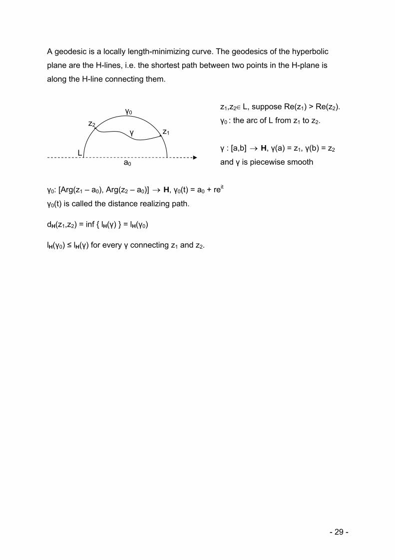
A geodesic is a locally length-minimizing curve. The geodesics of the hyperbolic

plane are the H-lines, i.e. the shortest path between two points in the H-plane is

along the H-line connecting them.

z1,z2∈L, suppose Re(z1) > Re(z2).

z1

z2

. .

γ0

L a0

γ

γ0 : the arc of L from z1 to z2.

γ : [a,b] → H, γ(a) = z1, γ(b) = z2

and γ is piecewise smooth

γ0: [Arg(z1 – a0), Arg(z2 – a0)] H, γ→ 0(t) = a0 + reit

γ0(t) is called the distance realizing path.

dH(z1,z2) = inf { lH(γ) } = lH(γ0)

lH(γ0) ≤ lH(γ) for every γ connecting z1 and z2.

- 29 -

References:

[1] Lars V. Ahlfors, Complex analysis, 3rd Ed, McGraw-Hill, 1979,

ISBN 0-07-000657-1

[2] H.A. Priestley, Complex analysis, 2nd Ed, Oxford University Press,

2003, ISBN 0-19-852562-1

[3] Dennis G. Zill, Patrick D. Shanahan, A first course in complex analysis with applications, Jones and Bartlett Publishers, 2003,

ISBN 0-7637-1437-2

[4] Stephen D. Fisher, Complex variables, 2nd Ed,

Wadsworth & Brooks/Cole, 1990, ISBN 0-534-13260-X

[5] A. David Wunsch, Complex variables with applications, 2nd Ed,

Addison-Wesley, 1994, ISBN 0-201-12299-5

[6] James W. Anderson, Hyperbolic geometry, Springer-Verlag, 1999,

ISBN 1-85233-156-9

- 30 -