Vision Res. Vol. 32, No. 7, pp. 1271-1284, I992 0042.6989192 $5.00 + 0.00

Printed in Great Britain. All rights reserved Copyright CT: 1992 Pergamon Press Ltd

The Optics of the Spherical Fish Lens W. S. JAGGER*

Received I7 October 1991

The optical design of the fish eye is particularly simple because immersion renders the cornea optically ineffective and the lens is nearly spherical in shape. Measurements have shown that an approximately parabolic gradient of refractive index exists within the lens. If full internal and external spherical symmetry of the lens applies, the geometrical-optical. behaviour of the lens is then a function only of the refractive index of the surrounding medium, that of the lens core and cortex, and of the form of the index gradient. The theoretical optical performance of models of the spherical fish lens is calculated by means of the ray-tracing program Drishti as a basis for understanding the optical design of real fish and aquatic eyes. Models based on the gradients proposed by earlier workers are shown to be unable to predict reported spherical aberration and image quality. A model of the fish lens with a poiynomial gradient is proposed that yields spherical aberration, image quality and chromatic aberration similar to that reported for the fish.

Fish Lens Optics Model Refractive index gradient Image quality Spherical aberration Chromatic aberration

INTRODUCTION

In the fish eye, the lens alone must perform the task of producing a good retinal image because immersion renders the cornea optically ineffective. The fish lens accomplishes this with two types of refractive processes. First, rays are refracted at the boundary of the lens with its surrounding homogeneous medium, at which a step of refractive index occurs. Second, rays within the lens follow curved paths, concave to the lens centre, as a result of its internal refractive index gradient. The first process is a function of the lens surface shape, and of the indices of the lens cortex and of the surrounding medium. The second process is a function of the cortical and core indices, and of the form of the gradient of refractive index. Compared to a homogeneous lens of the same paraxial power, this second process allows use of material of lower index, and it introduces additional degrees of design freedom that can allow the formation of an image of suitable quality.

The relative simplicity of the optics of the fish eye was recognised in the last century, and several treatments of a spherical inhomogeneous lens have appeared since. Maxwell (1854) considered a spherically symmetric lens of infinite size with an index gradient of the form:

n(u) = n(0)*aZ/(a’ + 72)

where n is refractive index, r is the distance from the centre, and a is a constant. He showed that this lens images points within it perfectly onto conjugate points opposite the centre such that object and image points lie on a diameter, the product of the object and image distances from the centre equals a’, and all rays within

*Department of Ecology and Evolutionary Biology, Monash

University, Clayton, Victoria 3168, Australia.

the lens follow circular paths. Although this lens is quite different from a fish lens, Maxwell conjectured that a finite sphere of this kind placed in water would offer a minimum of aberration, and that it might be possible to correct it chromatically.

Luneburg (1944) found a similar solution for a finite spherical lens, although he did not suggest it might apply to the fish lens. This lens, of unit radius, immersed in a homogeneous medium of index matching that of the lens cortex, forms a perfect image of a distant external object on the posterior surface of the lens. The Luneburg lens gradient has the form:

n(r)=J_

Fletcher, Murphy and Young (1954) found special solutions for the fish lens gradient, with infinite object distance and image placement outside the lens at various positions corresponding to the range observed in the fish eye. However, they also required that the cortical index match that of the surrounding medium. The gradients they present are solutions to an integral equation, and are expressed numerically.

Mattheissen (1882) measured the focal length (FL) of the lenses of ten fish species, and found that it averaged 2.55 times the lens radius (R), with variation between 2.40 and 2.82. This average value of the ratio FL/R, which corresponds to a relative aperture orf number of about f/l .275, has become known as Mattheissen’s ratio, and has generally been confirmed by others (Sadler, 1973), although Sroczyfiski (1975, 1976, 1977, 1978, 1979) found lower values for five species of fresh water fish between 2.19 for the roach and 2.44 for the pike. The full reported range of values of this ratio is therefore from 2.19 to 2.82, with individual species exhibiting smaller ranges. Mattheissen’s measurements (1880) of

1271

I271 W. S. JAGGER

index distribution within a lens of radius R by means of a refractometer on small samples showed an increase towards the centre that followed an approximately parabolic rule of the form:

n (r) = X0,, - (NC,,, - Nctx) . (r/R)*

Typical values he reported are 1.336 for the eye media (Nmed), 1.38 for the cortical index (No), and 1.51 for the core index (IV,,,). Mattheissen used the concept of total index, which is that index a homogeneous lens would require to have the same paraxial focal length as an inhomogeneous lens of the same shape. He showed mathematically that a spherical lens with a parabolic gradient of index can achieve the same power as a homogeneous lens of the same shape if the value of its core index lies halfway between the cortex index and the total index. When applied to real lenses, Mattheissen’s ray formulas did not predict aplanatic performance, and he (Mattheissen, 1893) explored means to improve their predictive ability. He suggested an elliptical gradient form which yielded less spherical aberration than the parabolic gradient, but still showed strong undercorrec- tion for rays incident near the edge of the lens.

Fernald and Wright (1983) claimed that the fish lens had a large homogeneous index core of 0.674 of the lens radius on the basis of the behaviour of laser beams refracted by intact and partially peeled lenses. However, Campbell and Sands (1984) disputed their conclusions, and argued that such a lens would be afflicted with unacceptably large spherical aberration. They showed by means of ray tracing that a gradient of refractive index should exist throughout the lens. Axelrod, Lerner and Sands (1988) measured the entrance and exit apertures of a series of laser beams passing through goldfish lenses. They concluded that the refractive index gradient inside the lens was smooth, with a form similar to the parabola of Mattheissen. Their estimates of core and cortical indices lay in the range 1.55-1.57 and 1.36-1.38.

Further detailed measurements of focal length and spherical aberration for rays incident at six zones, or distances from the central incident ray (Sroczynski, 1975, 1976, 1977, 1978, 1979) show that the isolated fish lens is well corrected except for the outer zones, which tend toward over-correction, and then swing sharply toward undercorrection at the highest zones. He found the entrance aperture radius of fish lenses to be about 0.95 of the radius. Sivak and Kreuzer (1983), on the basis of measurements at two or three zones, found undercor- rection in goldfish and perch and better correction in the rock bass. Pumphrey (1961) reported he was unable to detect chromatic aberration in the fish, but measure- ments by Sroczynski show a large paraxial chromatic focal length difference between 436 and 630 nm of about 4.5% for the brown trout (Sroczynski, 1978) and the perch (Sroczynski, 1979), and 5% for the rainbow trout (Sroczynski, 1976). Mandelman and Sivak (1983) also reported strong chromatic aberration in the rock bass. The highest reported behaviourally determined visual acuity measurements show that the tuna can discrimi- nate a grating of 8 c/deg (Nakamura, 1968), while the

range of acuities reported for other fish decreases from this to about one-quarter this value (Douglas & Hawryshyn, 1990).

This work presents calculations of the optical proper- ties of the spherically symmetric model fish lens with realistic values of core, cortex and surrounding medium indices as a basis for understanding the optical design of real fish and aquatic eyes.

METHODS

The general case of the optics of a gradient index lens in a homogeneous medium is too complex to allow exact analytic solutions describing ray trajectories to be found, although Mattheissen (1880, 1893) found approximate solutions for the case of the spherical fish lens with parabolic, Maxwellian and elliptical index gradients in a medium of index below that of the lens cortex. However, numerical methods used to trace ray paths through the lens can predict the optical behaviour of specific cases to any desired accuracy. The program Drishti (Sands, 1984), developed to calculate the optical properties of eyes (Hughes, 1986), was used to trace rays through the inhomogenous spherical model fish lens of unit radius. This program has been used to calculate optical properties of models of the rat eye (Campbell & Hughes, 1981), the cat lens (Jagger, 1990), the cat eye (Jagger, Sands & Hughes, 1992) and the human eye (Jagger & Hughes, 1989). Correct function of this program was assured by conventional checks, including the prediction of zero aberration of the original Luneburg lens. Spheri- cal aberration was calculated by tracing a meridional fan of incident rays through the lens. Aberrations that are functions of field angle, such as third-order coma, third-order oblique astigmatism, and lateral chromatic aberration do not occur in a spherically symmetric system, and can be neglected when treating the lens alone. The size of the image at best focus is found by minimising the root-mean-square radius (R,,) of a pencil of rays. This radius is a measure of the width of the point spread function (if this function is a Gaussian, R,, is equal to 0.86 of the radius at half-maximum), and is an inverse measure of image quality. Terminology used is that of modern optical engineering (Smith, 1966). According to this usage, the spherical aberration of a biconvex glass lens is negative, or undercorrected. This sign convention differs from that of some optometric literature.

RESULTS

The image surface of the spherical fish lens is spherical and concentric with the lens (although some real fish retinas deviate from this shape), and the important aberrations are spherical aberration and longitudinal chromatic aberration. Spherical aberration is expressed here as longitudinal spherical aberration. This is measured as the distance from the paraxial focus to the crossing of two rays that are parallel before encountering the lens, the first of which passes through the lens centre

OPTICS OF THE SPHERICAL FISH LENS 1273

and is undeviated, while the second ray is incident upon the lens at a zone located height h from the central ray.

Refractive index values within the fish lens have been measured by Mattheissen (1880, 1885) and Axelrod et al. (1988), and typical values at 589 nm to be used here for a model lens are N,&, 1.336; N,,,, 1.38; and I?,,, 1.52.

The gradients proposed by Maxwell (1854), Luneburg (1944) and Fletcher et al. (1954) can be adapted to the case of the fish lens, although the fish lens differs from the original conditions for which these gradients were derived. Maxwell’s infinite lens did not consider refrac- tion at the fish lens boundary. Also, an infinitely distant object would have been imaged infinitesimally small, as the rule of image formation of the Maxwell lens differs from that of more conventional lenses. The Luneburg lens also does not account for refraction at the lens boundaries, and its image lies on the lens posterior surface. The gradient of Fletcher et al. places object and image at appropriate locations, but the lens cortical index is that of the surrounding medium.

Model fish lenses of unit radius incorporating the Maxwell, Luneburg, Fletcher et al. and Mattheissen (I 880, 1893) gradients must inco~orate boundary con- ditions requiring the index at r = 0 to equal the core index, and that at Y = 1 to be equal to the cortical index. The final forms of these gradients are then:

Maxwell

n(r) = X0,*[1/(1 f KlZl.X-r*)l

where K,,, = (NC,, /NC,, ) - 1;

Luneburg

n (r ) = [NC,, . $--Tc7li,ii-

where i(l,,,, = J2-11 - (~~~~/~~~~~~I;

Fletcher, Murphy and Young

n(r) = N,.,,;(l + 0.6218*K*r2 + 1.8075eK*r4

- 7.2453.K# + 14.2087.K.r*

- 12.7280.K.ri0 + 4.3353.K.r12).

The numerical solution these authors present for a focal length of 2.5 times the lens radius has a core index 1.1371 times the cortical index, which equals the medium index. The more realistic case examined here, of core and cortical indices 1.52 and 1.38, with medium index 1.336, demands this ratio to be 1.1014. To achieve this, their gradient was truncated at radius 0.9404, and fit to a twelfth-degree polynomial where the polynomial co- efficients were found by least squares fitting and

K = (X,, PC,,) - 1.

Mattheissen parabola

n(r) = N,,,.(l + K.r2).

Mattheissen ellipse (fit to an eighth-degree polynomial)

n(r) = N,,,;(l + 0.85683+K.r’+ 0.08978.K.r’

+ 0.04495.K.r6 + 0.00841*K,r81.

u Lens radius

1 .o

FIGURE 1. Fish lens model refractive index gradients. The ordinate

is refractive index, and the abscissa is distance from the centre of a lens

of unit radius. From left to right, the curves represent the Maxwell,

Mattheissen parabola, Luneburg, Mattheissen ellipse, improved poly-

I

It is possible to find, by an optimisation procedure adjusting polynomial coefficients, an improved fish lens index gradient that takes surface refraction into account, with realistic object and image distances. This gradient, expressed as a polynomial, reduces the total spherical aberration to a small value up to the 0.95 zone for the index values given above:

n(r) = N,,,,(l + 0.8200.K*r”

+ 0.3000.K*rh - 0.1200*K+rx)

where K = (NC,, /IV,,,,) - 1.

Spherical symmetry requires that these gradients be independent of the sign of r and hence only even powers of r appear in their poIynomia1 expressions. While the parabolic gradient proposed by Mattheissen can be described as 100% second-degree polynomial, the im- proved gradient consists of 82% second-degree, 30% sixth-degree, and 12% eighth-degree polynomial terms. The gradient of Fletcher et al. (1954) is described by a twelfth-degree polynomial, with large coe~cients of both signs.

Figure 1 shows the shapes of the various gradients treated here. From left to right, in order of increasing

Ncore

N

Ncortex

nomial, and Fletcher el al. gradients.

1274 W. S. JAGGER

1.56

Ncore

1.52

1.48

1.643

1.56

NCOW

1.52

1.48

L MaxweIl

/

1.34

/ I I

1.38 Ncortex 1.42

(c 1

‘-I -, ---.

1 -I 3sp,

_

t ) Luneburg -

t /

1.34 1.38 Ncortex 1.42

Ncore

1.52

1.48

1.60

1.56

1.52

1.48

lb)

i __ /--I lid, Mattheissen parabola

I / I

1.34 1.38 Ncortex 1.42

(d)

;--”

I i

;’ _... c r.__ -.-

i -t ,

ic------ i I i

/ _.__.-- c

I

/---- _

f c F---T,

? .

1

t / /

i

7

:- ’ I

7 i

, i I

7 ’ --,

’ i f

‘i \ ‘\\ I

/

Mattheissen ellipse

/ I L’ , / I

1.34 1.38 Ncortex 1.42

Fig 2. (a-d) Capiion on facing page.

OPTiCS OF THE SPHERICAL FISH LENS 1275

1.60

1.56

NCOW

1.52

I .48

1.34 1.38 Ncortex 1.42

Ncore

I .52

I .48

Fletcher et al.

I I / I

1.34 1.28 Ncortex 1.42

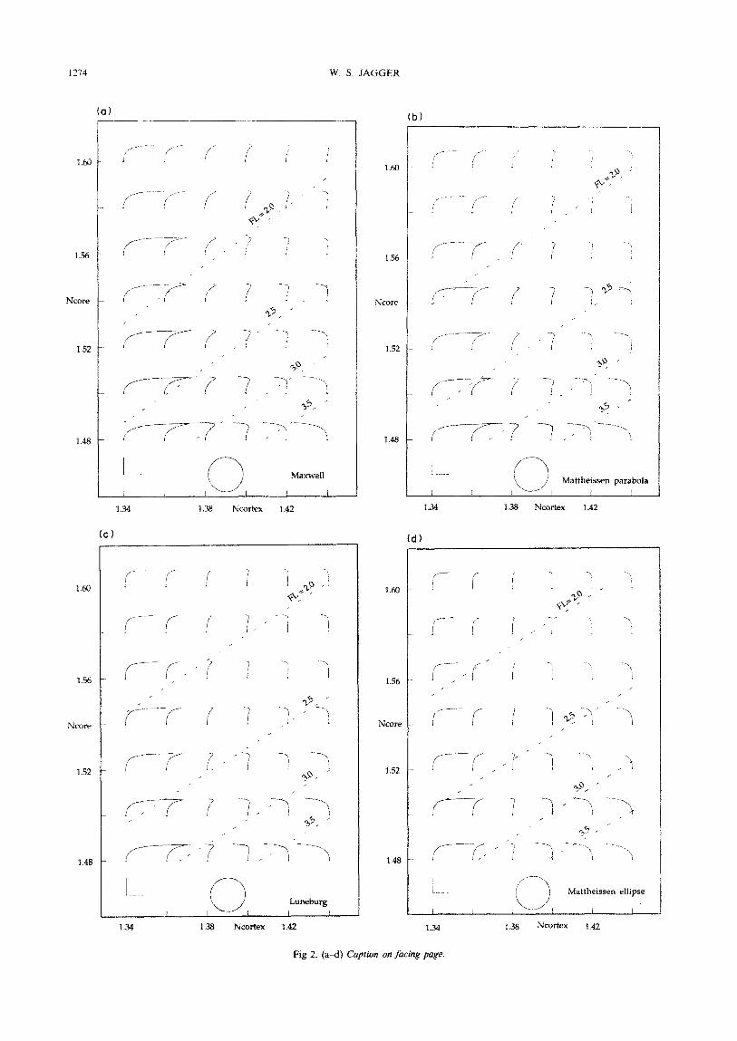
FIGURE 2. Individual curves of longitudinal spherical aberration up to incident ray height 0.975 for various values of core and cortical index of the model fish lens. For each curve. the unit length calibration bars for aberration (horizontal) and lens zone (vertical) are identical (lower left), and the circular outline of the lens of unit radius to which they apply is also shown below at the same scale. This set of curves is plotted in the plane of core index (ordinate) and cortical index (abscissa). Dashed lines indicate constant paraxial focal length. Refractive index gradients used in each lens model are: (a) Maxwell, (b)

Mattheissen parabola, (c) Luneburg, (d) Mattheissen ellipse, (e) improved polynomial gradient, (f) Fletcher et al.

area under each curve, they are the gradients of Maxwell, Mattheissen (parabola), Luneburg, Mattheis- sen (ellipse) the improved polynomial, and Fletcher et al. If a particular gradient form and surrounding medium index is assumed, only the lens parameters N,, and NC,, are free, and it is possible to map the spherical aberration curves for each gradient as a function of these two parameters in the plane they define (Fig. 2). Also shown in these figures are lines defining constant paraxial focal lengths.

The general behaviour of spherical aberration over this plane is similar for these gradients. At low Nftx, overcorrection of spherical aberration occurs, while at high NC,, , this aberration becomes undercorrected. In the intermediate region, however, instead of complete correction, complex curves appear for each gradient. As N EOE is increased, the magnitude of the aberration decreases, although complete correction does not occur for any pair of NC,, and N,,,, . However, for the improved polynomial gradient, this complex curve is nearly straight at the index values of interest, except for the highest zone, indicating better image quality. The lines of constant paraxial focal length show that the focal length decreases as N,,, increases, and increases as NC,, increases. VR 3217-E

For the core and cortical indices 1.52 and 1.38, the paraxial focal length for each gradient increases during the progression of curves from left to right in Fig. 1: 2.38 (Maxwell), 2.44 (Mattheissen parabola), 2.48 (Luneburg), 2.55 (Mattheissen ellipse), 2.59 (improved polynomial) and 2.68 (Fletcher et cd.). Also, the spherical aberration at a specific value of core and cortical index shifts from overcorrection to undercorrection as the area under the gradient curve increases, During this progression, the lines of constant paraxial focal length shift upward.

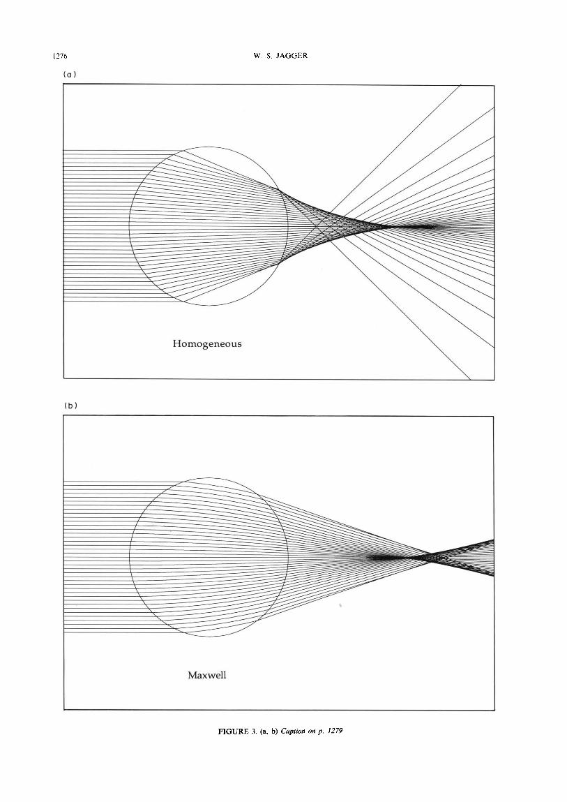
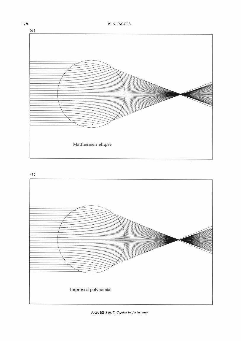
Figure 3 shows ray paths through models of a spheri- cal homogeneous lens of paraxial focus length 2.5 and index 1.67 (the total index of Mattheissen) and of spherical lenses possessing Maxwell, Mattheissen, Luneburg, improved polynomial, and Fletcher et al. gradients for NCOre 1.52 and NC, 1.38. Mattheissen’s prediction that the core index (1.52) lies halfway between the total index (1.67) and the cortical index (1.38) is nearly confirmed. Image quality for the homogeneous lens is clearly very poor and for the Maxwell, Mattheis- sen parabola, and Luneburg gradients it is poor, although somewhat better for the Mattheissen ellipse and the gradient of Fletcher et al. The best imaging occurs for the improved polynomial gradient lens.

I276 W. S. JAGGER

(a)

Homogeneous

(b)

Maxwell

FIGURE 3. (a, b) Caption on p. 1279

OPTICS OF THE SPHERICAL FISH LENS

(cl

Mattheissen parabola

(d 1

Luneburg

FIGURE 3. (c, d) ~~pti~~ on p. 1279

127X W. S. JAGGER

(e)

Mattheissen ellipse

Improved polynomial

FIGURE 3 (e, f) Caprion on facing page.

OPTICS OF THE SPHERICAL FISH LENS 1279

(cl)

Fletcher et al.

FIGURE 3. Ray paths through model lenses incorporating different refractive index gradients. Rays are spaced at incident ray height intervals of 0.05, up to 0.95. The lens model core index is I .52, and the cortical index is 1.38, except for the homogeneous model, of index 1.67. (a) Homogeneous; (b) gradient of Maxwell; (c) parabolic gradient of Mattheissen; (d) gradient of Luneburg; (e) elliptical gradient of Mattheissen; (f) improved polynomial gradient; (g) gradient of Fletcher et nl.

Figure 4(a) is a logarithmic plot of the rms radius (R,,) of the focussed image of an infinitely distant point object as a function of pupil radius up to 0.95 for the improved polynomial gradient, and for those of Maxwell, Luneburg, ~attheissen and Fletcher er al. The horizontal line at R,, 2 min of arc corresponds to the estimated R,, required to permit the highest reported acuity for the fish, 8 c/deg in the tuna. This estimate is based on equating twice the R,, to one-half the period of the grating detected. This is somewhat arbitrary, and a larger R,, may also be acceptable, depending on the contrast discrimination ability of the animal. The improved polynomial gradient offers this R,, at 0.93 and smaller pupil radius, while the other gradients permit this resolution only for pupils stopped to much smaller diameters.

As the object moves closer, the size of the best focussed image for pupil size 0.95 increases and hence image quality decreases for the six gradients considered [Fig. 4(b)]. The fractional increase is small for the Naxwell, ~attheissen and Luneburg gradients as the object moves in to 10 times the lens radius. The improved polynomial gradient shows a more rapid increase in focussed image size as the object distance becomes small, but its curve still remains well below those of the other gradients.

Figure 5(a) shows the longitudinal spherical aberra- tion curve of the improved polynomial gradient lens model, while Fig. 5(b) shows the change to this curve upon increase of the index of the surrounding medium by 0.003 to 1.339. This increase in index corresponds approximately to a doubling of solute concentration. Overcorrection of the lens results, with degradation of the focussed R,, at 0.95 pupil aperture from 2.7 to 5.4min of arc.

A small shape change in the lens has little effect on its optical behaviour. Figure 5(c) shows the longitudinal spherical aberration of a lens shortened axially by 2%, becoming an oblate spheroid. In a plane containing the axis, the originally circular surface curves and internal isoindicial curves become ellipses. The R,, at 0.95 pupil dia increases slightly from 2.7 to 2.8 min of arc.

The curve of Fig. 5(d) is the spherical aberration of the improved polynomial lens with a model fish cornea of constant thickness 0.2 {in units of the lens radius), anterior radius 2.0, located 0.3 anterior of the lens and having index 1.4. This cornea causes slight overcorrec- tion, and the curve is coincident with that of the lens flattened axially by 2%. The R,, at the 0.95 zone also increases from 2.7 to 2.8 min of arc.

The chromatic aberration of the fish lens is a function of the dispersion of the surrounding medium and of the

W. S. JAGGER

30

R=%

arc min

IO

////I /Mktheissen ellipse /

// Improved polynomiali

0 0.2 Il.4 0.6 0.8

Pupil Radius

(a)

I

ca

I I I

too0 ICQ 10 object Distance

(b)

FIGURE 4. (a) Root-mean-square image radius (R,) of each model as a function of pupil radius for each lens model type. The horizontal line indicates R,, = 2 arc min. the approximate value required for the highest acuity reported for a fish, 8 c,/deg (tuna, Nakamura. 1968). (b) R,, as a function of object distance (expressed in lens radii) for each lens model gradient for

a pupil radws of 0.95.

OPTICS OF THE SPHERICAL FISH LENS 1281

I /

0.2 / I

0.2 / I /

FIGURE 5. Sensitivity of the longitudinal spherical aberration of the fish lens model with the improved polynomial gradient to small changes in the index of the medium, to a small axial shortening, and to the presence of a cornea. (a) Unaltered improved polynomial model. (b) Immersed in medium of index 1.339, an increase of 0.003. (c)

1 I I

Shortened axially by 2%. (d) With a cornea of index 1.4.

lens substance. Jagger (1990) measured the dispersion curves of cat lens substance, which do not extend to the high index of the fish lens core. Sivak and Mandelman (1983) also measured lens dispersion for various animals. Srocyznski (1976) measured the longitudinal chromatic aberration of the rainbow trout, and found a difference in focal length of about 5% between 440 and 640nm. Assuming that the dispersion of fish lens cortical substance is the same as that of the cat, it is possible to find the dispersion curve of fish lens core substance that results in the chromatic aberration found by Srocyznski. Figure 6(a) shows the dispersion curves of the surround- ing medium, of cat lens cortical substance of index 1.38 at 589 nm, and of fish lens core material of index 1.52 at 589 nm calculated to yield the chromatic aberration observed by Sroczynski. The Abbe number, an inverse measure of dispersion (Smith, 1966), is 55 for the medium, 50 for the cortex, and 38 for the lens core. Using a similar procedure, it is possible to calculate the hypothetical lens core dispersion curve that would yield a lens free of longitudinal chromatic aberration. The broken line shows this dispersion curve, with Abbe number 68.

Figure 6(b) shows the curve of longitudinal chromatic aberration calculated for a model lens possessing these dispersions. The chromatic aberration reported by Scroczynski (1976) for the rainbow trout lens is indicated by points on this curve. The broken line shows the

variation of paraxial focal length with wavelength of a lens with the hypothetical dispersion of Fig. 6(a) chosen to correct chromatic aberration.

DISCUSSION

Image quality of the lens models

The lens gradients of Maxwell and Luneburg fail to produce a sharp image when applied to a realistic model of the fish lens. Because they were originally conceived for other object and image locations, and do not con- sider the refraction at the boundary of the lens with the surrounding medium, the resulting spherical aberration causes poor image quality. Fletcher et al. (1954) claimed

2.M1

FL

2.56

2.48

1.54

1.52

1.50

.

.

1.40

N

1.38

1.3h

1.34

tbl

(al

Cortex

Medium

I 450

I I 5co 550 Wavelength, nm

I I 600 650

FIGURE 6. (a) Dispersion curves for the model fish lens with the improved polynomial gradient. The curve of the bathing medium is that of water at 20°C (Houstoun, 1934), increased by 0.003 to account for salt content, yielding 1.336 at 589 nm. The dispersion curve of the lens cortex is a second-order fit to data measured on the cat lens from Jagger (1990), with value 1.38 at 589 nm. The core dispersion curve is calculated to yield the fish longitudinal chromatic aberration reported by Sroczynski (19X), whose measured points are shown in (b). The dashed line is the dispersion curve of core substance that would be required to correct lon~tudinal chromatic aberration. The solid curve of(b) is the paraxial focal length of the model fish lens calculated using the dispersion curves of (a). Points shown on this curve are those measured by Sroczynski (1976) for the rainbow trout. The dashed line is the paraxial focal length of a model lens with the hypothetical core dispersion curve shown in (a) that results in correction of longitudinal

chromatic aberration

12x2 W. S. JAGGER

that their own gradient offered good image quality for a fish lens with realistic object and image locations, with, however, cortical index equal to that of the medium. This neglect of refraction at the step of index at the boundary of the real lens also results in uncorrected spherical aberration and inadequate image quality. Mattheissen (1880) chose his parabolic gradient because it offered a simple description of his limited data. However, this gradient also fails to produce adequate image quality, either because his data were insufficiently accurate or his fit to the data was not good enough. It would be a remarkable coincidence if a simple parabolic gradient produced good image quality in this complex system; in general more degrees of design freedom would be required. Mattheissen (1893) realised this, and explored the optics of an elliptical gradient. This gradient yields better image quality than the parabolic gradient, but still leaves room for improvement.

The form of the improved polynomial index gradient, which yields acceptable image quality, differs relatively little from these other gradients (Fig. 1). and high precision index measurements would be required to distinguish between them. The improved polynomial gradient was found by using the additional degrees of freedom offered by a polynomial function of higher degree to minimise spherical aberration. Although the power contributed by refraction at the lens surface is only about one-sixth the power contributed by the gradient, the components of spherical aberration from each process are of similar magnitude and opposite sign and result in a small total abe~ation. However, spherical aberration becomes undercorrected even for this gradi- ent near the edge of the lens. Because this aberration changes so rapidly near the lens edge, light is spread over a large area, causing broad veiling rather than widening of the point image. In addition, internal reflection and scattering can be expected to minimise the effects of these edge rays, limiting the entrance pupil radius to about 0.95 (Sroczynski, 1975). The fish iris is usually immobile, and the pupil is nearly the same size as the lens. If the iris were slightly smaller than the lens diameter, it would also cut off these edge rays.

Measured spherical aberration and focal length, and the behaviour of the lens model with the improved polynomial gradient

Several features of the optical behaviour of the model fish lens with the improved gradient agree with detailed measurements reported by Sroczynski for five species of fresh water fish (pike, 1975; rainbow trout, 1976; Roach, 1977; brown trout, 1978; perch, 1979). All the spherical aberration curves he measured show a sharp hook to undercorrection near the highest zone (about 0.95), and all but the pike show overcorrection at high zones (about 0.7-0.95). This behaviour is displayed by the model fish lens [Fig. 5(a)], The size of the deviation of the measured spherical aberration curves from a straight line is about 2% of the focal length (excepting the undercorrected hook at high zones). The model fish lens exhibits a figure about a third this size, and corresponds to the high

acuity reported for the tuna; a larger aberration is readily produced by altering the model gradient slightly to degrade its performance. In addition, Sroczynski found that as the measured ratio FL/R decreases, the correction of spherical aberration improves, and the sharp hook to undercorrection occurs at a higher zone. The value of FL/R is inversely related to the size of the animal (pike) and to the lens size (perch).

These relations between FL/R, spherical aberration and the zone at which the undercorrected hook occurs can be understood in terms of the model lens if it is assumed that lens core index increases as the animal grows, as has been observed in the cat (Jagger, unpub- lished observations), perhaps as a result of increasing core dehydration. Figure 2(e) then shows that as the core index of the model fish lens increases, FL/R also decreases, its spherical aberration becomes better corrected, and the hook towards undercorrection occurs at higher zones. Sroczynski (1979) found that as the perch lens grew from 1.7 to 5.7 mm dia, FL/R decreased from 2.5 to 2.3, with a decrease in spherical aberration. Figure 2(e) indicates that in the model fish lens, this decrease in FL/R with concomitant improvement in spherical aberration would result from an increase in NC,, of about 0.025.

Sensitivity of lens performance to optical parameters

The spherical aberration and hence image quality of the model fish lens is very sensitive to index gradient shape and cortical index, while it is less sensitive to core index, a small variation in lens shape, realistic variation in medium index, and the presence of a cornea (Figs 2 and 5). For the model lens of core index 1.52 and cortical index 1.38, the progression through the gradient forms of Fig. 1 in the direction of curves with increasing convexity (from left to right) results in overcorrected spherical aberration progressing to undercorr~tion~ with an optimal intermediate form, the improved poly- nomial gradient. A feedback mechanism sensing retinal image quality and controlling lens refractive structure may exist, and it is possible to speculate about how this might function. The relatively dense core of the fish lens would be expected to hold a nearly constant index over periods short compared to the animal’s life, while the metabolically more active cortical layers would also maintain a constant cortical index by active control of their water content. If the cortical cells perform a gatekeeper role to control the total amount of water within the lens, this water might be partitioned by a radially increasing concentration of hydrophilic groups in the concentric fibre layers of the lens to form the smooth gradient of index. Decreasing the total amount of water in the lens would cause the curve to become more convex and vice versa, allowing fine tuning of the gradient shape and hence image quality. Fine tuning of lens image quality in this manner would require a control signal originating in the retinal mosaic, with the goal of maintaining some degree of cone undersampling throughout growth (Snyder, Bossomaier & Hughes, 1986).

OPTICS OF THE SPHERICAL FISH LENS 1283

Although the improved polynomial gradient described

here was optimised for only one set of medium, core and

cortical indices, its spherical aberration and hence image

quality is relatively insensitive to core index [Fig. 2(e)], and it is reasonable to expect that the medium index does not change greatly in different cases. Different optimal gradients for real fish lenses need then only occur for different values of cortical index. Slightly different gradi- ents for other index values have been found that offer similar optical performance, and it is likely that a gradient offering adequate image quality exists for any

set of realistic index values.

Chromatic aberration and the resulting image degradation

The chromatic aberration of the fish lens is quite large, in contradiction to Maxwell’s speculation that it might be corrected. Correction of longitudinal chromatic aberration could be achieved if, instead of a core Abbe number of 38, as calculated to yield the observed chromatic focus difference, the core substance had much less dispersion, with Abbe number about 68 (Fig. 6). This would require lens material dispersion to decrease with index. The large magnitude of the aberration is

apparently the result of lens material whose dispersion increases with index. Similar increase in dispersion with increasing index was reported for various animals (Sivak & Mandelman, 1983) and for the cat (Jagger, 1990).

Although the core substance is solid, its index value of 1.52 and Abbe number 38 place it outside the range of

glasses (Smith, 1966). The retinal image of a white point of light can be focussed for only one wavelength. Its image will consist of a series of concentric disks corresponding to each out-of-focus wavelength. The effect of this image degradation will depend upon ocular absorbing pigments (Muntz, 1976) and photoreceptor pigment absorption spectra of the animal, and its central integration of colour information. Sunlight that reaches fish at any significant depth becomes more blue and narrowed in spectral bandwidth because of absorption and scattering (Lythgoe, 1979) and this effect will also decrease the impact of high lens chromatic aberration.

Focal length and image quality of the lens during growth

The design of the spherical fish lens is independent of its absolute size; that is, the lens of unit radius treated here may be of any real dimension, and its geometrical- optical behaviour will remain the same, offering the same image quality, expressed in c/deg. However, as a real lens grows, it does not necessarily scale perfectly, and the ratio of the focal length to the lens radius (FL/R), and the image quality may not remain constant. In addition, the spacing of the retinal receptor elements may change during growth.

Baerends, Bennema and Vogelzang (1960) reported that during growth of a cichlid fish, linear cone spacing remained nearly constant, behavioural acuity increased, while lens size increased and FL/R decreased somewhat. This decrease in FL/R is similar to that reported by Sroczynski (1975, 1979) discussed above. Hairston, Li and Easter (1982) also found that the linear spacing of

sunfish cones changed little during growth, while

behaviourally measured acuity increased. Apparently

the growing fish uses the increasing focal length and

hence increasing linear image size of the growing eye together with constant linear cone spacing to improve its

acuity. However, during growth in the cat, potential acuity measured by angular subtense of retinal beta- ganglion cell dendritic trees remains constant outside the

area centralis, but increases within the area centralis (Wong & Hughes, 1988).

Less is known about image quality during growth. In

the cat, Bonds and Freeman (1978) found that image quality increased rapidly during the first weeks of life before stabilising at the adult value. Some undersam-

pling by the cone mosaic might be expected in the adult animal (Snyder et al., 1986). In the fish, if the image quality (expressed in c/deg) remains constant during

growth, and the cone linear spacing does not change, young fish must tolerate much more cone undersam- pling, and photoreceptors would be more readily visible

(Jagger, 1985; Land & Snyder, 1985) in young animals than in older animals.

If image quality is controlled during growth by an

open loop system (with no feedback), this case may apply. However, if information from the cone mosaic is used in a closed loop system to control image quality and maintain constant retinal sampling, the image quality of the lens may improve with growth. This follows because of the coarse angular spacing of the mosaic (in cones/deg) in the young animal, and the finer spacing in the older animal. Information required to produce a lens of high image quality in the young lens would not be available because of the coarse cone spacing.

Very small lenses will be affected by diffraction, a physical-optical effect, which limits angular resolution to about 30 c/deg per mm of entrance aperture diameter. A fish lens able to resolve 8 c/deg would be diffraction limited if it were less than about 0.3 mm in diameter.

REFERENCES

Axelrod, D., Lerner, D. & Sands, P. J. (1988). Refractive index within

the lens of a goldfish eye determined from the paths of thin laser

beams. Vision Research, 28, 57-65. Baerends, G. P., Bennema, B. E. & Vogelzang, A. A. (I 960). ijber die

Anderung der Sehscharfe mit dem Wachstum bei Aequidens

portalegrensis (Hensel) (Pisces, Ciclidae). Zoologische Jahrhiicher (Physiologic), 88, 67-78.

Bonds, A. B. & Freeman, R. D. (1978). Development of optical quality

in the kitten eye. Vision Research, 18, 391-398. Campbell, M. C. W. & Hughes, A. (1981). An analytic, gradient index

schematic lens and eye for the rat which predict aberrations for finite

pupils. Vision Research, 21, 1129-I 148. Campbell, M. C. W. & Sands, P. J. (1984). Optical quality during

crystalline lens growth. Nature, 312, 291-292. Douglas, R. H. & Hawryshyn, C. W. (1990). In Douglas. R. H. &

Djamgoz, M. B. A. (Eds), The visual .xystem qffish (pp. 373418). London: Chapman & Hall.

Fernald, R. D. & Wright, S. E. (1983). Maintenance of optical quality

during crystalline lens growth. Nature, 301. 618420. Fletcher, A., Murphy, T. & Young, A. (1954). Solutions of two optical

problems. Proceedings of the Royal Society of London A, 223, 216-225.

I284 W S. JAGGER

Hairston. N. G. Jr, Li, K. T. & Easter, S. S. Jr (1982). Fish vision and the detection of planktonic prey. Science, 218, 1240-1242.

Houstoun, R. A. (1934). A rreofire on light. London: Longmans, Green.

Hughes, A. (1986). The schematic eye comes of age. In Pettigrew, J. G.. Sanderson. K. J. & Levick, W. R. (Eds), Vi.wu/ neuroscierwe

(pp. 60-89). Cambridge: Cambridge University Press. Jagger. W. S. (1985). Visibility of photoreceptors in the intact living

cane toad eye. Vision Research, 2s. 729-73 I. Jagger, W. S. (1990). The refractive structure and optical properties of

the isolated crystalline lens of the cat. Vision Research, 30, 723-738.

Jagger, W. S. & Hughes, A. (1989). An aspheric gradient index model of the human eye. Neuroscience Letters (Suppl.), 34, SIOO.

Jagger, W. S., Sands. P. J. & Hughes, A. (1992). Wide-angle, aspheric. gradient index modelling of the optics of the cat eye. In preparation.

Land, M. F. & Snyder, A. W. (1985). Cone mosaic observed through natural pupil of live vertebrate. Vision Reseurch, 25. 1519.-I 523.

Luneburg, R. K. (1944). Mathematical theory of oprics. Berkeley. Calif.: University of California Press.

Lythgoe. J. N. (1979). The ecology of vision. Oxford: Clarendon Press. Mandelman, T. & Sivak, J. G. (1983). Longitudinal chromatic aberra-

tion of the vertebrate eye. Vision Research. 2-3. 1555-1559. Mattheissen, L. (1880). Untersuchungen iiber den Aplanatismus und

die Periscopie der Krystalllinsen in den Augen der Fische. Pptigers

Archiv, 21, 287-307.

Mattheissen. L. (I 882). Ueber die Beziehungen, welche zwischen dem Brechungsindex des Kerncentrums der Krystalllinse und den Dimen- sionen des Auges bestehen. Pfliigers Archiv. 27, 510-523.

Mattheissen. L. (1885). Ueber Begriff und Auswerthung des sogenan- nten Totalindex der Krystalllinse. Pptgers Archiv, 36. 72. 100.

Mattheissen, L. (1893). X. Beitrige zur Dioptrik der Krystall-Linse. Zeitschrifr fir vergleichende Augenheilkunde. 7, IO2 146.

Maxwell, J. C. (1854). Solutions of problems. Cambridge and Dublin

Mathematical Journal, 8, 188-195. Reprinted in Niven. W. D. (Ed.), The scientific papers of James Clerk Maxwell (Vol. I) 1890. Cambridge: Cambridge University Press.

Muntz, W. R. A. (1976). The visual consequences of yellow filtering pigments in the eyes of fishes occupying different habitats. In Evans. G. C.. Bainbridge, R. & Rackham, 0. (Eds), Light us an ecological

fucror: II. Oxford: Blackwell.

Nakamura, E. L. (1968). Visual acuity of yellowtin tun;t. I’~runmc.~ albucares. FAO Fi.sh Report. 62. 463 468.

Pumphrey, R. J. (1961). Concerning vision. In Ramsey. J. A. L Wigglesworth, V. 8. (Eds), T/I~ (,el/ und orgunism. C‘ambridgc: Cambridge University Press.

Sadler. J. D. (1973). The focal length of the fish eye lens and visual acuity. Vision Reseurch, 1.7. 417 423.

Sands, P. J. (1984). Drishti. a computer program ior analysing sym- metrical optical systems incorporating inhomogeneous media. Tech- nlcal Report 8, Canberra: CSIRO Divison of Computing Research.

Sivak, J. G. & Kreuzer. R. 0. (1983). Spherical aberration of the crystalline lens. Vi.Gon Research. 2.1, 59-70.

Sivak. J. G. & Mandelman, T. (1983). Chromatic dispersion of the ocular media. Vi.Gon Reseurch, 22. 997 1003.

Smith. W. J. (1966). .Cfodern opt~cul engineertng. New York: McGraw Hill.

Snyder, A. W.. Bossomaier, 1. R. J. & Hughes. A. (1986). Optical image quality and the cone mosaic. Science. 231. 499. 501.

Sroczyfiski. S. (1975). Die sphlrische Aberration der Augenlinse des Hechts (E.sos iuc2u.s L.). Zoologishc Juhrhiicher (Physiologic). 79.

547 558.

Sroczy6ski. S. (1976). Die chromatische Aberration der Augenlinse der Regenbogenforelle (Salmo gairdneri Rich.). Zoologische Jahrbticher

(Physiologic). 80. 432450.

Sroczytiski. S. (1977). Spherical aberration of crystalline lens in the roach. Rutilus rutilur L. Journal of Comparative Physiology A, 121.

135 144.

Sroczyriski, S. (I 978). Die chromatische Aberration der Augenlinse der Bachforelle (Salmo truttu furio L.). Zoologishe Jahrhiicher (Physiolo-

gie). 82, 113-133. Sroczyriski, S. (1979). Das optische System des Auges des

Flussbarsches (Percu @viatilis L.). Zoologische Jahrbiicher (Physi-

ologic), 83. 224 -252.

Wong, R. 0. L. & Hughes. A. (1988). Development of visual resolution in the cat retina. Neuroscience Lvtters (SuppI.). 30. Sl41.

Acknowledgements--The author wishes to thank W. R. A. Muntz and A. Hughes for helpful discussions. This work was supported by Australian Research Council Grant No. A09031258 and the Ema and Victor Hasselblad Foundation.