the pauli-lubanski vector in a group-theoretical … · the pauli-lubanski vector in a...
TRANSCRIPT
The Pauli-Lubanski Vector in a Group-Theoretical Approach
to Relativistic Wave Equations
by
Nathan A. Lanfear
A Dissertation Presented in Partial Fulfillmentof the Requirements for the Degree
Doctor of Philosophy
Approved June 2016 by theGraduate Supervisory Committee:
Sergei Suslov, Co-ChairBrett Kotschwar, Co-Chair
Rodrigo PlatteDmitry Matyushov
Hendrik KuiperCarl Gardner
ARIZONA STATE UNIVERSITY
August 2016
ABSTRACT
Chapter 1 introduces some key elements of important topics such as; quantum mechanics,
representation theory of the Lorentz and Poincare groups, and a review of some basic rela-
tivistic wave equations that will play an important role in the work to follow. In Chapter 2,
a complex covariant form of the classical Maxwell’s equations in a moving medium or at
rest is introduced. In addition, a compact, Lorentz invariant, form of the energy-momentum
tensor is derived. In chapter 3, the concept of photon helicity is critically analyzed and its
connection with the Pauli-Lubanski vector from the viewpoint of the complex electromag-
netic field, E+ iH. To this end, a complex covariant form of Maxwell’s equations is used.
Chapter 4 analyzes basic relativistic wave equations for the classical fields, such as Dirac’s
equation, Weyl’s two-component equation for massless neutrinos and the Proca, Maxwell
and Fierz-Pauli equations, from the viewpoint of the Pauli-Lubanski vector and the Casimir
operators of the Poincare group. A connection between the spin of a particle/field and
consistency of the corresponding overdetermined system is emphasized in the massless
case. Chapter 5 focuses on the so-called generalized quantum harmonic oscillator, which
is a Schrodinger equation with a time-varying quadratic Hamiltonian operator. The time
evolution of exact wave functions of the generalized harmonic oscillators is determined
in terms of the solutions of certain Ermakov and Riccati-type systems. In addition, it is
shown that the classical Arnold transform is naturally connected with Ehrenfest’s theorem
for generalized harmonic oscillators. In Chapter 6, as an example of the usefulness of the
methods introduced in Chapter 5 a model for the quantization of an electromagnetic field
in a variable media is analyzed. The concept of quantization of an electromagnetic field
in factorizable media is discussed via the Caldirola-Kanai Hamiltonian. A single mode
of radiation for this model is used to find time-dependent photon amplitudes in relation
to Fock states. A multi-parameter family of the squeezed states, photon statistics, and the
uncertainty relation, are explicitly given in terms of the Ermakov-type system.
i

“Physical laws should have mathematical beauty.” — P. A. M. Dirac
ii

ACKNOWLEDGMENTS
Sincere thanks go to my fiancee for being so supportive during this time! I would also
like to thank my mother, sister, and all my siblings and family, who live far across the coun-
try, for being so understanding of my occasional visits, which were usually far too short,
during this long endeavour. Many sincere thanks go to my outstanding mentor, Dr. Sergei
Suslov who has helped to transform me from a very curious student into a researcher. His
help in organizing conferences at which I made valuable connections was much appreci-
ated, and so was his help in obtaining support. Thanks also go to my co-advisor, Dr. Brett
Kotschwar, who on many occasions has given me valuable advice and encouragement.
Many thanks go to all my committee members for their helpful comments and suggestions
over the years. I would also like to thank ASU, the School of Mathematical and Statistical
Sciences, and our director Dr. Al Boggess for an extraordinary amount of support. All of
this has helped tremendously in my research and has helped me to attend conferences to
share my projects. Many thanks to Dr. Svetlana Roudenko for all her encouragement over
the years, for helping to organize wonderful conferences and workshops, and for helping to
secure support. Thanks also go to my advisor’s former students whose work has guided my
own to some extent and whose encouragement has been invaluable to my success. Thanks
also go to Dr. Gerald Goldin for his encouraging comments and suggestions regarding
work I presented at a conference in Munich, Germany. All of these people and many others
have been outstandingly helpful! Many thanks to Renate Mittelmann for all her technical
support, which has without a doubt been essential. Last but not least, thanks also go to
Debbie Olson and Jennifer May for help with many organizational details over the years
that helped to keep me and many other students on track. My apologies to anyone I have
not listed; a number of people have contributed to my success over the years and I thank
you all very much!
iii

TABLE OF CONTENTS
CHAPTER Page
1 INTRODUCTION . . . . . . . . . . . . . . . . . . . . . . . . . . . . . . . . . . . . . . . . . . . . . . . . . . . . . . 1
1.1 Notation . . . . . . . . . . . . . . . . . . . . . . . . . . . . . . . . . . . . . . . . . . . . . . . . . . . . . . . . . . 2
1.2 A Brief Discussion on Quantum Mechanics . . . . . . . . . . . . . . . . . . . . . . . . . . 4
1.3 Representation Theory and the Lorentz and Poincare Groups . . . . . . . . . . 6
1.3.1 Homogeneous Lorentz Group . . . . . . . . . . . . . . . . . . . . . . . . . . . . . . . 7
1.3.2 Inhomogeneous Lorentz (Poincare) Group . . . . . . . . . . . . . . . . . . . . 9
1.4 A Brief Review of Some Relativistic Wave Equations . . . . . . . . . . . . . . . . . 10
1.4.1 Klein-Gordon-(Fock) Equation . . . . . . . . . . . . . . . . . . . . . . . . . . . . . . 10
1.4.2 Dirac Equation . . . . . . . . . . . . . . . . . . . . . . . . . . . . . . . . . . . . . . . . . . . . . 12
1.4.3 Weyl Equation . . . . . . . . . . . . . . . . . . . . . . . . . . . . . . . . . . . . . . . . . . . . . 14
1.4.4 Maxwell Equation . . . . . . . . . . . . . . . . . . . . . . . . . . . . . . . . . . . . . . . . . . 15
1.4.5 Proca Equation . . . . . . . . . . . . . . . . . . . . . . . . . . . . . . . . . . . . . . . . . . . . . 17
1.4.6 Einstein Equation . . . . . . . . . . . . . . . . . . . . . . . . . . . . . . . . . . . . . . . . . . 18
2 COMPLEX ELECTRODYNAMICS . . . . . . . . . . . . . . . . . . . . . . . . . . . . . . . . . . . . . 20
2.1 Maxwell’s Equations in 3D-Complex Form . . . . . . . . . . . . . . . . . . . . . . . . . . 21
2.2 Hertz Symmetric Stress Tensor . . . . . . . . . . . . . . . . . . . . . . . . . . . . . . . . . . . . . 22
2.3 “Angular Momentum” Balance . . . . . . . . . . . . . . . . . . . . . . . . . . . . . . . . . . . . . 27
2.4 Complex Covariant Form of Macroscopic Maxwell’s Equations . . . . . . . . 28
2.5 Dual Electromagnetic Field Tensors . . . . . . . . . . . . . . . . . . . . . . . . . . . . . . . . . 30
2.6 Covariant Derivation of Energy-Momentum Balance Equations . . . . . . . . 32
2.6.1 Preliminaries . . . . . . . . . . . . . . . . . . . . . . . . . . . . . . . . . . . . . . . . . . . . . . 32
2.6.2 Proof . . . . . . . . . . . . . . . . . . . . . . . . . . . . . . . . . . . . . . . . . . . . . . . . . . . . . 33
2.7 Covariant Derivation of Angular Momentum Balance . . . . . . . . . . . . . . . . . 35
2.8 Transformation Laws of Complex Electromagnetic Fields . . . . . . . . . . . . . 36
iv
CHAPTER Page
2.9 Material Equations, Potentials, and Energy-Momentum Tensor for Mov-
ing Isotropic Media . . . . . . . . . . . . . . . . . . . . . . . . . . . . . . . . . . . . . . . . . . . . . . . . 40
2.9.1 Material Equations . . . . . . . . . . . . . . . . . . . . . . . . . . . . . . . . . . . . . . . . . 40
2.9.2 Potentials . . . . . . . . . . . . . . . . . . . . . . . . . . . . . . . . . . . . . . . . . . . . . . . . . . 42
2.9.3 Hertz’s Tensor and Vectors . . . . . . . . . . . . . . . . . . . . . . . . . . . . . . . . . . 43
2.9.4 Energy-Momentum Tensor . . . . . . . . . . . . . . . . . . . . . . . . . . . . . . . . . . 45
2.10 Real vs Complex Lagrangians . . . . . . . . . . . . . . . . . . . . . . . . . . . . . . . . . . . . . . 45
2.10.1 Complex Forms . . . . . . . . . . . . . . . . . . . . . . . . . . . . . . . . . . . . . . . . . . . . 46
2.10.2 Real Form . . . . . . . . . . . . . . . . . . . . . . . . . . . . . . . . . . . . . . . . . . . . . . . . . 47
2.11 Formulas from Vector Calculus . . . . . . . . . . . . . . . . . . . . . . . . . . . . . . . . . . . . . 48
2.12 Dual Tensor Identities . . . . . . . . . . . . . . . . . . . . . . . . . . . . . . . . . . . . . . . . . . . . . 49
2.13 Proof of Identities (2.63) . . . . . . . . . . . . . . . . . . . . . . . . . . . . . . . . . . . . . . . . . . . 51
3 THE PAULI-LUBANSKI VECTOR AND PHOTON HELICITY . . . . . . . . . . . 53
3.1 Transformation Laws and Generators . . . . . . . . . . . . . . . . . . . . . . . . . . . . . . . . 54
3.2 The Pauli-Lubanski Vector and Maxwell’s Equations in Vacuum . . . . . . . 56
3.3 Examples . . . . . . . . . . . . . . . . . . . . . . . . . . . . . . . . . . . . . . . . . . . . . . . . . . . . . . . . . 58
3.4 Helicity . . . . . . . . . . . . . . . . . . . . . . . . . . . . . . . . . . . . . . . . . . . . . . . . . . . . . . . . . . 60
3.5 Covariant Harmonic Wave Solutions . . . . . . . . . . . . . . . . . . . . . . . . . . . . . . . . 62
3.6 Discrete Transformations and Polarization . . . . . . . . . . . . . . . . . . . . . . . . . . . 63
4 PAULI-LUBANSKI VECTOR AND RELATIVISTIC WAVE EQUATIONS . 66
4.1 Dirac Equation . . . . . . . . . . . . . . . . . . . . . . . . . . . . . . . . . . . . . . . . . . . . . . . . . . . . 69
4.1.1 Gamma Matrices, Bispinors, and Transformation Laws . . . . . . . . 69
4.1.2 Generators and Commutators . . . . . . . . . . . . . . . . . . . . . . . . . . . . . . . . 73
4.1.3 Balance Conditions and Energy-Momentum Tensors . . . . . . . . . . . 74
v
CHAPTER Page
4.1.4 Variants of Dirac’s Equation . . . . . . . . . . . . . . . . . . . . . . . . . . . . . . . . . 75
4.1.5 Covariance and Transformation of Generators . . . . . . . . . . . . . . . . . 77
4.1.6 Hamiltonian and Energy Balance . . . . . . . . . . . . . . . . . . . . . . . . . . . . 79
4.1.7 The Pauli-Lubanski Vector and Dirac’s Equation for a Free Par-
ticle . . . . . . . . . . . . . . . . . . . . . . . . . . . . . . . . . . . . . . . . . . . . . . . . . . . . . . . 79
4.1.8 Relativistic Definition of Spin for Dirac Particles . . . . . . . . . . . . . . 80
4.2 Weyl Equation for Massless Neutrinos . . . . . . . . . . . . . . . . . . . . . . . . . . . . . . . 81
4.2.1 Rotations, Boosts, and their Generators . . . . . . . . . . . . . . . . . . . . . . . 82
4.2.2 The Pauli-Lubanski Vector and Weyl’s Equation . . . . . . . . . . . . . . . 83
4.2.3 Covariance . . . . . . . . . . . . . . . . . . . . . . . . . . . . . . . . . . . . . . . . . . . . . . . . 84
4.2.4 An Alternative Derivation . . . . . . . . . . . . . . . . . . . . . . . . . . . . . . . . . . . 86
4.3 Proca Equation . . . . . . . . . . . . . . . . . . . . . . . . . . . . . . . . . . . . . . . . . . . . . . . . . . . . 87
4.3.1 Massive Vector Field . . . . . . . . . . . . . . . . . . . . . . . . . . . . . . . . . . . . . . . 87
4.3.2 An Alternative “Bispinor” Derivation . . . . . . . . . . . . . . . . . . . . . . . . 89
4.3.3 Maxwell’s Equations vs Proca Equation . . . . . . . . . . . . . . . . . . . . . . 90
4.4 Complex Vector Field . . . . . . . . . . . . . . . . . . . . . . . . . . . . . . . . . . . . . . . . . . . . . . 90
4.4.1 Vector Covariant Form . . . . . . . . . . . . . . . . . . . . . . . . . . . . . . . . . . . . . . 91
4.4.2 Commutators . . . . . . . . . . . . . . . . . . . . . . . . . . . . . . . . . . . . . . . . . . . . . . 92
4.4.3 Lorentz Invariance . . . . . . . . . . . . . . . . . . . . . . . . . . . . . . . . . . . . . . . . . 93
4.4.4 Vector Covariant Form vs Traditional Form of Maxwell’s Equa-
tions . . . . . . . . . . . . . . . . . . . . . . . . . . . . . . . . . . . . . . . . . . . . . . . . . . . . . . 93
4.4.5 An Alternative Form of Maxwell’s Equations . . . . . . . . . . . . . . . . . 94
4.5 On Spinor Forms of Maxwell’s Equations . . . . . . . . . . . . . . . . . . . . . . . . . . . . 95
4.5.1 Spinor Covariant Form. . . . . . . . . . . . . . . . . . . . . . . . . . . . . . . . . . . . . . 96
vi
CHAPTER Page
4.5.2 Traditional Spinor Form of Maxwell’s Equations . . . . . . . . . . . . . . 97
4.6 Massive Symmetric Four-tensor Field . . . . . . . . . . . . . . . . . . . . . . . . . . . . . . . 98
4.6.1 Group-Theoretical Derivation . . . . . . . . . . . . . . . . . . . . . . . . . . . . . . . 98
4.6.2 An Alternative Gauge Condition . . . . . . . . . . . . . . . . . . . . . . . . . . . . . 101
4.6.3 Fierz-Pauli vs Maxwell’s Equations . . . . . . . . . . . . . . . . . . . . . . . . . . 102
4.6.4 Fierz-Pauli vs Linearized Einstein’s Equations . . . . . . . . . . . . . . . . 103
4.7 Summary . . . . . . . . . . . . . . . . . . . . . . . . . . . . . . . . . . . . . . . . . . . . . . . . . . . . . . . . . 104
5 WAVE FUNCTIONS FOR GENERALIZED HARMONIC OSCILLATORS . 105
5.1 Transforming Generalized Harmonic Oscillators into Autonomous Form 106
5.2 Green’s Function and Wavefunctions . . . . . . . . . . . . . . . . . . . . . . . . . . . . . . . . 108
5.3 Solution to Ermakov-type System . . . . . . . . . . . . . . . . . . . . . . . . . . . . . . . . . . . 110
5.4 Solution of the Ermakov-type Equation . . . . . . . . . . . . . . . . . . . . . . . . . . . . . . 113
5.5 Ehrenfest Theorem Transformations . . . . . . . . . . . . . . . . . . . . . . . . . . . . . . . . . 114
5.6 Conclusion . . . . . . . . . . . . . . . . . . . . . . . . . . . . . . . . . . . . . . . . . . . . . . . . . . . . . . . 115
6 A MODEL FOR RADIATION FIELD QUANTIZATION IN MEDIA . . . . . . . 116
6.1 Exact Wave Functions and the Ermakov-type System . . . . . . . . . . . . . . . . . 118
6.2 The Uncertainty Relation and Squeezing . . . . . . . . . . . . . . . . . . . . . . . . . . . . . 119
6.3 Photon Statistics . . . . . . . . . . . . . . . . . . . . . . . . . . . . . . . . . . . . . . . . . . . . . . . . . . 121
REFERENCES . . . . . . . . . . . . . . . . . . . . . . . . . . . . . . . . . . . . . . . . . . . . . . . . . . . . . . . . . . . . . . . 125
vii
Chapter 1
INTRODUCTION
In this chapter we will briefly review some important topics that are relevant to this
dissertation. No attempt has been made to give a complete and detailed description of each
area, but instead to just introduce and discuss certain aspects of the theories that will be
most relevant in the work to follow.
In section 1.1, we introduce some notations that will be used throughout. In section
1.2, we will briefly review some important fundamentals of quantum mechanics including:
Hamiltonians, the Schrodinger equation, the Heisenberg uncertainty principle, Ehrenfest’s
Theorem, and the unitary transformation between the Schrodinger and Heisenberg pictures
of quantum mechanics. In section 1.3, the representation theory of the Poincare and Lorentz
groups will be discussed. This will be very important in the sections on relativistic wave
equations and spin and angular momentum of elementary particles. Section 1.4 gives a
brief review of several fundamental relativistic wave equations that will be visited again in
relation to the Pauli-Lubanski vector and the representation theory of the Poincare group in
a later chapter.
In Chapter 2, a complex version of electrodynamics is introduced. We discuss a com-
plex covariant form of the classical Maxwell’s equations, in a moving medium or at rest. A
compact, Lorentz invariant, form of the energy-momentum tensor is derived.
Chapter 3 addresses a common misconception in the literature and the standard quan-
tum field theory textbooks on an operator relation used to define helicity of massless parti-
cles. In accomplishing this, it is shown that Maxwell’s equations in vacuum can, in fact, be
derived through the representation theory of the Poincare group with the help of the Pauli-
Lubanski vector. The definition of helicity, as it is traditionally given in particle physics, is
1
discussed and the simplest covariant helicity states are constructed. The chapter concludes
with some remarks regarding polarized waves and a discussion on the complex Maxwell
equations in vacuum and discrete transformations.
Chapter 4 emphasizes the role of the Pauli-Lubanski vector for several major relativistic
wave equations. The work in this chapter was motivated by a result of Chapter 3, that
Maxwell’s equation can be derived through the representation theory of the Poincare group
with the help of the Pauli-Lubanski vector. The chapter begins by introducing a variant
version of Dirac’s equation, which takes the form of a certain overdetermined system of
partial differential equations. Next, there is a discussion on the Pauli-Lubanski vector and
Dirac’s equation in vacuum, and lastly the relativistic definition of spin for Dirac particles.
The chapter continues on to cover, in a similar manner, the Weyl, Proca, Maxwell, and
Fierz-Pauli equations. In addition, the spinor form of Maxwell’s equations is mentioned in
a covariant form, along with its traditional form.
In Chapter 5, we change gears to discuss the exact wave functions for a generalized
harmonic oscillator, which is a Schrodinger equation whose Hamiltonian is a general time-
dependent quadratic operator of position and momentum. Green’s function is found with
help from the Ermakov-type system, which is also introduced in this chapter. The chapter
concludes by outlining Ehrenfest’s theorem and how it relates to the generalized harmonic
oscillators.
Lastly, in Chapter 6, an application of the results from Chapter 5 helps to study a certain
model for the quantization of an electromagnetic field in variable media. The exact wave
function for the model is found, the uncertainty relation and squeezed states are discussed,
and lastly the photon statistics are explicitly given.
1.1 Notation
• Natural units, where the fundamental constants c = h = 1, will generally be used.
2

• Latin indices i, j,k, ... run over spatial coordinate labels, i, j,k = 1,2,3.
• Greek indices µ,ν ,ρ, ... run over the four spacetime coordinate labels µ,ν ,ρ =
0,1,2,3.
• The flat Minkowski spacetime metric tensor is denoted ηµν = diag(1,−1,−1,−1).
• The curved spacetime metric tensor is denoted gµν , but in most places we are work-
ing in flat spacetime where this notation is used to indicate the Minkowski metric
instead. Any place such a notation is used it will be indicated.
• The the totally anti-symmetric Levi-Civita symbol in three and four dimensions is
denoted by epqr and eµνστ , respectively. The convention e123 = +1 and e0123 = +1
is used.
• Three-dimensional spatial vectors are indicated by a boldface letter, e.g. A.
• A contravariant four-vector is denoted with an upper index xµ and a covariant four-
vector with a lower index xµ .
• The relation between contravariant and covariant vectors is given by the metric ten-
sor, xµ = ηµνxν .
• The spacetime interval ds2 = dxµdxµ = dt2−dx2−dy2−dz2.
• The four-gradient operator is denoted ∂µ =(
∂
∂ t ,∇)=(
∂
∂ t ,∂
∂x ,∂
∂y ,∂
∂ z
).
• For the contravariant four-gradient ∂ µ = ηµν∂ν =(
∂
∂ t ,−∇
).
• The d’Alembert operator is = ηµν∂µ∂ν = ∂µ∂ µ = ∂ 2.
• The four-momentum of a particle is given by pµ = (E,p).
• Sometimes the notation p · x = px = pµxµ = Et−p ·x is used.
3

1.2 A Brief Discussion on Quantum Mechanics
In classical mechanics, the Hamiltonian,
H(p,x) = T +V where T = T (p) =p2
2mand V =V (x), (1.1)
represents the total energy of a closed system. Here the functions T (p) and V (x) represent
the kinetic and potential energies respectively. The variable p represents the generalized
momenta and x the generalized coordinates. These state variables depend on time and the
time evolution of the system is given by the Hamilton equations,
x =∂H∂ p
=pm
(1.2)
p =−∂H∂x
=−dV (x)dx
. (1.3)
The variables p and x completely describe the state of the system. The equations (1.2)-
(1.3) are derived from the Lagrangian formalism of classical mechanics, see any standard
classical mechanics text for details.
In quantum mechanics, the Hamiltonian is obtained by replacing the variables p and
x by the operators p= hi
∂
∂x and x= x. These are operators on an infinite dimensional Hilbert
space, which is the setting of quantum mechanics. It is a postulate of quantum mechanics
that the state of the quantum system at time t is given by a wavefunction ψ (x, t), which is
represented by a vector in an infinite dimensional Hilbert space. The time evolution of the
quantum system is given by the Schrodinger equation,
ih∂ψ (x, t)
∂ t= Hψ (x, t) where H =
p2
2m+V (x). (1.4)
Here the kinetic and potential energies are given in terms of the operators p and x.
4
A general variable quadratic Hamiltonian,
H = a(t)p2 +b(t)x2 + c(t)x p− id(t)− f (t)x−g(t)p, (1.5)
where a, b, c, d, f and g are suitable real-valued functions of time t only, will be discussed
later. In most places it will be clear from the context when we are dealing with an opera-
tor and for this reason the hat, O, above operators will usually be left out. A measurable
quantity, often called an observable, in quantum mechanics corresponds to a self-adjoint
operator, and the possible outcomes of measurements to values in the spectrum of the oper-
ator. The action of an operator on a wave function yields an eigenvalue, when it exists, that
corresponds to the particular quantity being measured. Examples of such operators include
the position, momentum, and energy operators. The expectation value of an operator with
respect to a normalized quantum state ψ gives the statistical mean of the measurements
performed on ψ:
〈A〉=∞∫−∞
ψ∗AψdV.
The Heisenberg uncertainty principle is of great importance to quantum mechanics, in gen-
eral: given two non-commuting self-adjoint operators A and B such that [A,B] = ih, the
following inequality is satisfied
〈∆A〉〈∆B〉 ≥ h/2, (1.6)
where 〈∆A〉=√〈A2〉−〈A〉2 and 〈∆B〉=
√〈B2〉−〈B〉2 is the uncertainty, or standard de-
viation, of the respective operators. Typically, this statement is given for the position A = x
and momentum B = p operators; although, this relation holds true for any conjugate oper-
ators that satisfy the given hypothesis. As a result, this statement says that if the measured
value of one of the operators, say A, is known precisely, then the value of the operator B
is infinitely uncertain. There are especially important quantum states that minimize the
relation (1.6), known as coherent states or, more generally, squeezed coherent states. The
5
term squeezed is used to described the coherent states whose oscillating variances⟨(∆A)2⟩
and⟨(∆B)2⟩ become smaller than the ’static’ vacuum state, for which
⟨(∆A)2⟩ =
⟨(∆B)2⟩
= h/2. The Ehrenfest theorem gives the time-evolution of the expectation value of an oper-
ator, A, according to the formula
ddt〈A〉= 1
ih〈[A,H]〉+
⟨∂A∂ t
⟩.
Finally, one may move back and forth between the Schrodinger and Heisenberg pictures of
quantum mechanics, transferring the time-dependence from the wave functions to the op-
erators or vice versa, using a unitary transformation. The equivalence of these two pictures
of quantum mechanics will be useful below when calculating the photon statistics. In the
Heisenberg picture of quantum mechanics the state vectors are time-independent, while the
observable operators instead depend on time and satisfy the Heisenberg equation of motion
ddt
A(t) =ih[H,A(t)]+
(∂A∂ t
)H. (1.7)
The subscript on the last term, ∂A∂ t indicates that it has undergone the unitary transformation
along with the operator A
A(t) = eiHt/hAe−iHt/h,
for a time-independent Hamiltonian. For a time-dependent Hamiltonian a more general
unitary operator should be used, see [118]. Note that taking the expectation value of the
Heisenberg equation yields the Ehrenfest theorem.
1.3 Representation Theory and the Lorentz and Poincare Groups
The purpose of this section is to introduce some notations that will be used in the work
to follow, along with a brief review of some important topics regarding the Lorentz and
Poincare groups and their representations. The main body of work takes place in the
Minkowski space MMM = (R4,g), where g = gµν = diag(1,−1,−1,−1) is the Minkowski
6

metric. When working in a curved spacetime we instead reserve the symbol g for the met-
ric tensor and use instead the symbol η for the Minkowski metric. A reminder of many of
the notations will be given in the sections as they are needed, although a list has already
been provided in the introduction. A classification program for relativistic wave equa-
tions through the representation theory of the inhomogeneous Lorentz (Poincare) group was
started by Bargmann and Wigner in 1948, [12]. Chapter 4 follows the work of Bargmann
and Wigner with a classification program of relativistic wave equations from the represen-
tation theory of the Poincare group, where these equations appear in this framework as a
statement of consistency of certain overdetermined systems of partial differential equations.
In particular Dirac’s equation, Weyl’s two-component equation for massless neutrinos, and
the Proca, Maxwell and Fierz-Pauli equations are studied from the viewpoint of the Pauli-
Lubanski vector.
1.3.1 Homogeneous Lorentz Group
The Lorentz group O(1,3) is the group of all linear transformations of R4 that preserve
the Lorentz inner product xµyµ = gµνxνyµ . That is, given Λ ∈ O(1,3):
(Λx)µ(Λy)µ = gµν (Λνσ xσ )
(Λ
µ
κ yκ)= xµyµ for all x,y. (1.8)
Or in matrix form,
Λ†gΛ = g, (1.9)
where g is the Minkowski metric. The group O(1,3) has four connected components, which
can be seen by the following. Taking the determinant on both sides of the equation (1.9) it
is clear that detΛ = ±1. If detΛ = 1, the element Λ is called special. The equation (1.8)
implies that
Λµ
κ gµνΛνσ = gκσ , (1.10)
7
and setting κ = σ = 0 one gets
(Λ00)
2 = 1+3
∑j=1
(Λj0)
2 ≥ 1. (1.11)
This shows that we either have Λ00 ≥ 1 or Λ0
0 ≤ −1. The transformations Λ ∈ O(1,3)
such that Λ00 ≥ 1 are called orthochronous, meaning that they do not change the direction
of time. A special orthochronous Lorentz transformation is called proper. The set of
special transformations forms the special Lorentz group, denoted SO(1,3), and the set of
orthochronous transformations forms the orthochronous Lorentz group, O+(1,3). Then the
restricted Lorentz group (or proper Lorentz) group,
SO+(1,3) = SO(1,3)∩O+(1,3), (1.12)
is the connected component of the identity in O(1,3). The Lorentz group is a six-dimensional
Lie group and local coordinates may be introduced in it with the exponential map
Λ = exp(
θλ µmλ µ/2), (1.13)
where θλ µ is an anti-symmetric 4x4 matrix and the infinitesimal generators,(mλ µ
)α
β= gµα
δλ
β−gλα
δµ
β, mλ µ =−mµλ , (1.14)
satisfy the Lie algebra
[mλ µ ,mρσ ] = gλρmµσ −gµρmλσ +gµσ mλρ −gλσ mµρ . (1.15)
The universal covering of SO+(1,3) is a two-valued complex representation, denoted SL(2,C),
which is a connected Lie group. Representations of connected Lie groups can be studied
by algebraic methods. If T is any representation of SO+(1,3), where the elements of the
group have the form (1.13),
T (Λ) = exp(
iθλ µXλ µ/2), (1.16)
8

the linear operators Xλ µ = −X µλ are called the generators of the representation T , and
they satisfy the commutation relation of the Lie algebra,
[Xλ µ ,Xρσ ] =−i(
gλρX µσ −gµρXλσ +gµσ Xλρ −gλσ X µρ
). (1.17)
Finding all representations of the commutation rule (1.17) is equivalent to finding the
representations of the restricted Lorentz group, SO+(1,3). The restricted Lorentz group
has finite dimensional and infinite dimensional representations; however, it has no finite-
dimensional unitary representations other than the identity representation T (Λ) ≡ 1. In
the work to follow, we only concern ourselves with the finite-dimensional representa-
tions (four-vector, spinor, bispinor, four-tensor, etc...) of SO+(1,3), which act on finite-
dimensional vector spaces; elements of these spaces transform according to the correspond-
ing representation.
1.3.2 Inhomogeneous Lorentz (Poincare) Group
The Poincare group is the set of all homogeneous Lorentz transformations, O(1,3)
together with the group of translations, R4. That is, the ten-dimensional Lie group
P = R4 oO(1,3), (1.18)
which is why it is sometimes referred to as the inhomogeneous Lorentz group. The action
of an element (a,Λ) ∈P on x ∈ R4 is given by,
x′µ = Λ
µ
ν xν +aµ . (1.19)
As with the Lorentz group, the Poincare group also has four connected components. Similar
to the Lorentz group the component of the identity is
R4 oSO+(1,3), (1.20)
9

and the covering group is R4oSL(2,C). In addition to the generators in the Lie algebra for
the Lorentz group, the generator of translation, Pµ must be added to give the Lie algebra
of the Poincare group:
[Xλ µ ,Xρσ ] =−i(
gλρX µσ −gµρXλσ +gµσ Xλρ −gλσ X µρ
), (1.21)
[Pµ ,Pν ] = 0, (1.22)
[X µν ,Pσ ] = i(gνσ Pµ −gµσ Pν) . (1.23)
The classification of all the irreducible unitary representations of the inhomogeneous Lorentz
group can be formulated in terms of finding the all representations of the commutation rules
of this algebra by self-adjoint operators, see for example [231]. For more details on the
Lorentz and Poincare groups, see [15], [29], [187].
1.4 A Brief Review of Some Relativistic Wave Equations
1.4.1 Klein-Gordon-(Fock) Equation
The Klein-Gordon equation describes particles with no spin, which are called scalar
particles. We denote such a particle by φ , which has only one component. The Klein-
Gordon equation can be derived starting from the relativistic energy-momentum relation
(in units with h = c = 1),
E2−p2 = m2. (1.24)
Substituting the differential operators E → i ∂
∂ t and p→−i∇ in (1.24) and operating on φ
we obtain the Klein-Gordon equation,(∂ 2
∂ t2 −∇2)
φ +m2φ = 0, (1.25)
or in covariant form (+m2)
φ = 0. (1.26)
10

It should also be noted here, that since the Klein-Gordon equation expresses the relativistic
relation between energy, momentum, and mass, it must hold for particles of any spin. An-
other interesting fact is that the well-known Schrodinger equation, from quantum mechan-
ics, is the non-relativistic approximation to the Klein-Gordon equation, see for example
[184]. The four-vector jµ = (ρ, j), satisfies the continuity equation
∂µ jµ =∂ρ
∂ t+div j = 0, (1.27)
where
ρ =i
2m
(φ∗∂φ
∂ t− ∂φ∗
∂ tφ
)(1.28)
j =1
2im(φ∗∇φ − (∇φ)∗φ) , (1.29)
where the asterisk ∗ stands for complex conjugation. Here, we consider φ to be complex-
valued, which corresponds to charged particles. If instead φ were real-valued, (1.28)-(1.29)
would be identically zero. Real-valued φ corresponds instead to electrically neutral parti-
cles. However, the major problem here is that the quantity (1.28) is not positive-definite
since one can choose initial conditions on φ and ∂φ/∂ t to make it negative. Alternatively,
to see this, one may substitute a plane-wave φ = Ne−ipµ xµ
= Ne−i(Et−p·x) in (1.28) to find
that
ρ = 2|N|2E, (1.30)
from which it follows ρ may take negative values, since the energy E in (1.24) can be
positive or negative. Hence ρ cannot be interpreted as a probability density and one can
no longer interpret the Klein-Gordon equation as an equation for a single particle, [184].
This trouble with the Klein-Gordon equation is resolved by reinterpreting it instead as a
field equation for a field φ instead of a single particle. Upon quantization of the field
a successful particle theory may be recovered. The problem of negative energy, which
11

becomes a severe problem for an interacting particle, is also overcome by treating φ as a
quantum field.
1.4.2 Dirac Equation
The Dirac equation is a relativistic wave equation that was derived by Paul Dirac in
1928. The Dirac equation describes massive spin-1/2 particles such as, for example, elec-
trons, protons, and quarks. In its covariant form the Dirac equation is written
iγµ∂µψ−mψ = 0. (1.31)
Here the Dirac/gamma matrices are γµ =(γ0,γγγ
), γµ = gµνγν =
(γ0,−γγγ
), and γ5 =
−γ5 = iγ0γ1γ2γ3, where
γγγ =
0 σσσ
−σσσ 0
, γ0 =
I 0
0 −I
, γ5 =
0 I
I 0
(1.32)
and σσσ = (σ1,σ2,σ3) are the standard 2×2 Pauli matrices [168], [214]. The familiar anti-
commutation relations,
γµ
γν + γ
νγ
µ = 2gµν , γµ
γ5 + γ
5γ
µ = 0 (µ,ν = 0,1,2,3) , (1.33)
hold. (Most of the results here will not depend on a particular choice of gamma matrices,
but it is always useful to have an example in mind.) The four-vector notation, xµ = (t,r) ,
∂µ = ∂/∂xµ , and ∂ α = gαµ∂µ in natural units c = = 1 with the standard metric, gµν =
gµν = diag(1,−1,−1,−1) , in the Minkowski space-time (R4 ,g) are utilized throughout,
see [19], [28], [29], [157], [21].
In this notation, the transformation law of a bispinor wave function,
ψ (x) =
ψ1
ψ2
ψ3
ψ4
∈ C4 , (1.34)
12
under a proper Lorentz transformation, is given by
ψ′ (x′)= SΛψ (x) , x′ = Λx, (1.35)
together with the rule,
S−1Λ
γµSΛ = Λ
µ
νγν , (1.36)
for the sake of covariance of the Dirac equation (1.31).
As is well known, a general solution of the latter matrix equation has the form
S = SΛ = exp(−1
4θµνΣ
µν
), θµν =−θνµ , (1.37)
Σµν = (γµ
γν − γ
νγ
µ)/2.
For the conjugate bispinor,
ψ (x) = ψ† (x)γ
0, ψ′ (x′)= ψ (x)S−1
Λ, x′ = Λx, (1.38)
the Dirac equation (1.31) takes the form
i∂µψγµ +mψ = 0. (1.39)
(For more details see classical accounts [6], [19], [28], [71], [99], [158], [173], [184], [187],
[21], [226].) Using the two equations (1.31) and (1.39) on can easily show that the Dirac
current is conserved. Indeed, for the Dirac current jµ = ψγµψ = (ρ, j) one has
∂µ jµ = (∂µψ)γµψ +ψγµ(∂µψ)
= imψψ− imψψ = 0.
Thus showing the probability density and probability current are conserved for the Dirac
equation. A more general discussion of the conservation laws is given in Chapter 5. Note
that in the Dirac equation the probability density is positive,
ρ = j0 = ψγ0ψ = ψ
†ψ =
4
∑i=1|ψi|2 > 0.
13
However, the energy may still take positive or negative values in the Dirac equation. This
predicted the existence of an electron with positive charge called a positron, the antiparticle
of an electron, which was eventually discovered. Actually, Dirac’s theory predicted the
existence of antiparticles for all spin-1/2 particles. The existence of these antiparticles
necessitated the abandonment of the Dirac equation as a single-particle equation and for it
to instead be interpreted as a field equation, [184].
1.4.3 Weyl Equation
The Dirac equation can be written in terms of two Weyl spinors, φ and χ , under the
transformation,
γµ → γ
′µ = UγµU−1, ψ → ψ
′ =
φ
χ
=Uψ, (1.40)
U =1√2
I I
I −I
=U−1.
Through this transformation Dirac’s equation (1.31) takes a familiar block form,
i
0 ∂0−σσσ ·∇
∂0 +σσσ ·∇ 0
φ
χ
= m
φ
χ
(1.41)
(see, for example, [71], [158], and [173]). In the massless limit m→ 0, this system decou-
ples,
∂0φ +(σσσ ·∇)φ = 0, ∂0χ− (σσσ ·∇)χ = 0, (1.42)
resulting in Weyl’s two-component equations for massless neutrinos. This eponymous
equation was introduced by Hermann Weyl in 1929 to describe massless spin-1/2 parti-
cles, [187], [228]. Weyl’s equation was rejected because it was incompatible with parity
conservation, which reverses the sign of helicity, [99]. Later this objection was deemed
not serious since neutrinos are involved in weak interactions which do not conserve parity,
14
[131], [234]. It should be noted that the 2015 Nobel Prize in Physics was award to Arthur
B. McDonald and Takaaki Kajita for the discovery of neutrino oscillations, which shows
that neutrinos do have mass, see [149], [105], and [175] by Pontecorvo for the original
work on neutrino physics.
The Weyl equation can be written in a familiar covariant form, see [173], [187], [173],
by setting σ µ = (σ0 = I,σ1,σ2,σ3) and σ µ = (σ0 = I,−σ1,−σ2,−σ3) , to cast (1.42) into
the form:
σµ
∂µφ = 0, σµ
∂µφ = 0. (1.43)
Here, the Weyl spinors,
φ (x) =
φ1
φ2
∈ C2 , (1.44)
transform under the proper orthochronous Lorentz group as follows
φ′ (x′)= SΛφ (x) , x′ = Λx, SΛσ
µS−1Λ
= Λµ
ν σν , (1.45)
to ensure the covariance of the Weyl equation (1.43).
1.4.4 Maxwell Equation
In 1861, James Clerk Maxwell published his famous equations that now go by his name.
Maxwell’s equations together with the Lorentz force law form the foundation of classical
electrodynamics. In their 3D vector form Maxwell’s vacuum equations are given by
divB = 0, curlE+∂B∂ t
= 0 (1.46)
divE = ρ, curlB− ∂E∂ t
= j, (1.47)
where we have used Heaviside-Lorentz rationalized units. In this section we show how
Maxwell’s equations can be written in covariant form by following to some extent the
treatment in the quantum field theory textbook by Lewis H. Ryder, [184]. The divergence
15
equation in the homogeneous Maxwell equations (1.46) is a statement that there are no
magnetic charges and the second equation known as Faraday’s Law says that a changing
magnetic field induces an electric field. The divergence equation in the pair of inhomoge-
neous Maxwell equations (1.47), known as Gauss’s Law, says that the total charge inside a
closed surface may be obtained by integrating the normal component of E over the surface.
The second equation states that a current or a changing electric field generates a magnetic
field; this equation is Ampere’s Law with an additional time-derivative of E introduced by
Maxwell.
It is convenient to introduce the scalar potential φ and vector potential A that satisfy
B = curlA, E =−∂A∂ t−∇φ , (1.48)
and by which the homogeneous Maxwell equations (1.46) are automatically satisfied. Com-
bining these into the four-vector Aµ = (φ ,A) and defining
Fµν =−Fνµ = ∂µAν −∂
νAµ , (1.49)
one can verify that Fµν has the following block matrix form
Fµν =
0 −E p
Eq −epqrBr
(1.50)
or
Fµν =
0 −E1 −E2 −E3
E1 0 −B3 B2
E2 B3 0 −B1
E3 −B2 B1 0
,
where p,q,r = 1,2,3 and epqr = epqr is the three-dimensional totally anti-symmetric Levi-
Civita symbol with e123 = 1. The electromagnetic field tensor Fµν transforms under
Lorentz transformations as a second rank tensor:
F ′µν = Λµ
σ Λντ Fστ . (1.51)
16

Note also that Maxwell’s equations are invariant under the gauge transformation
Aµ → Aµ +∂ µ χ , where χ is a scalar function, which can be checked using (1.48) or (1.49).
The set of four equations (1.46)-(1.47) can be written as a pair of covariant tensorial equa-
tions; one is written in terms of the electromagnetic field tensor and the other one in terms
of its corresponding dual four-tensor which is defined by
Fµν =12
eµνστFστ =
0 −Bp
Bq −epqrEr
, (1.52)
where µ,ν ,σ ,τ = 0,1,2,3 and eµνστ =−eµνστ is the four-dimensional totally anti-symmetric
Levi-Civita symbol with e0123 = 1. Note that the dual four-tensor Fµν may be obtained
from Fµν by substituting E→ B and B→−E. In covariant form, Maxwell’s equations are
given by
∂µFµν = jν (1.53)
∂µ Fµν = 0, (1.54)
where jν = (ρ, j) is the four-current density. The equations (1.53) and (1.54) contain the
inhomogeneous (1.47) and homogeneous (1.46) Maxwell equations, respectively. Note that
in light of the antisymmetry of the Levi-Civita symbol, the equation (1.54) implies
∂λ Fµν +∂
µFνλ +∂νFλ µ = 0, (1.55)
It can be checked that this latter equation follows directly from (1.49). The familiar wave
equation for the four-potential Aµ under the choice of the Lorenz gauge, ∂µAµ = 0,
Aν = jν , (1.56)
is obtained by substituting (1.49) in (1.53).
1.4.5 Proca Equation
The Proca equations were introduced by Alexandru Proca in 1936, [176], to describe
massive spin-1 particles called massive vector bosons. The intermediate force particles
17
of the weak interaction, the W and Z bosons, are an example of such particles. Proca’s
equations generalize Maxwell’s equations and are given by
Fµν =−Fνµ = ∂µAν −∂
νAµ , ∂µFµν +m2Aν = jν , (1.57)
where jν = (ρ, j) is the four-current density. Proca’s equation is not invariant under the
gauge transformation, Aµ → Aµ + ∂ µ χ , where χ is a scalar function, as can be seen from
the mass term in (1.57). This gauge invariance is restored in the massless limit, m→ 0,
by which Proca’s equations are reduced to Maxwell’s equations. In addition, for the Proca
field, the Lorenz gauge condition,
∂µAµ = 0, (1.58)
always holds due to the antisymmetry of the electromagnetic field tensor and the conserva-
tion of four-current, ∂ν jν = 0. In light of this fact, one may combine equations (1.57) to
obtain:
Aν +m2Aν = jν , (1.59)
where = ∂µ∂ µ = ∂ 2
∂ t2 −∇2, is the d’Alembert operator. Once again, in the limit m→ 0,
this yields the equation (1.56). The condition (1.58) reduces the degrees of freedom by one
therefore leaving the four component potential Aµ with three independent components,
which one would expect for a massive particle.
1.4.6 Einstein Equation
In 1915, Albert Einstein first published his famous field equations and theory of general
relativity [59]. Einstein’s equation is a nonlinear tensorial equation that relates the curvature
of space-time to the energy-momentum tensor of matter in space-time:
Rµν −12
gµνR = 8πGTµν . (1.60)
Here, gµν is the symmetric metric tensor on a curved spacetime manifold, Tµν is the energy-
momentum tensor, Rµν the Ricci tensor, and R = gµνRµν is the Ricci scalar (the trace of
18
the Ricci tensor), for more details see, for example, [36], [37], [157]. Another useful form
of Einstein’s equation is obtained by taking the trace of (1.60) which yields R = −8πGT ,
so that
Rµν = 8πG(
Tµν −12
T gµν
). (1.61)
It follows from this that Einstein’s equation takes the following simple form in vacuum,
when Tµν = 0:
Rµν = 0. (1.62)
Note that in this section g refers to the metric tensor on a curved manifold, whereas η
will refer to the metric tensor ηµν = diag(1,−1,−1,−1) of the flat Minkowski spacetime.
This notation is useful when one wishes to linearize the Einstein equation about the flat
Minkowski spacetime metric – to analyze, for example, the Einstein equation in a weak
gravitational field. By considering only the first-order term in a series expansion of the
metric tensor gµν ,
gµν = ηµν +hµν , (1.63)
one obtains the linearized Einstein equation in vacuum
∂µ∂σ hσν +∂ν∂
σ hσ µ −∂µ∂νh (1.64)
−∂2hµν −ηµν
(∂σ ∂τhστ −∂
2h)= 0.
General relativity theory predicts the existence of gravitational waves, which can seen by
solving the linearized Einstein equation, [36]. In fact, the gravitational waves produced
from a binary black hole merger have recently been detected at LIGO, [1]. One should also
consider the massless spin-2 hypothetical particle, called the graviton, that corresponds to
gravitational waves. To describe such a particle a symmetric second rank tensor is needed.
A discussion for a massive spin-2 particle and its relation to the Einstein equation is pro-
vided in Chapter 5.
19

Chapter 2
COMPLEX ELECTRODYNAMICS
Although a systematic study of electromagnetic phenomena in media is not possi-
ble without methods of quantum mechanics, statistical physics and kinetics, in practice
a standard mathematical model based on phenomenological Maxwell’s equations provides
a good approximation to many important problems. As is well-known, one should be able
to obtain the electromagnetic laws for continuous media from those for the interaction of
fields and point particles [49], [47], [107], [124], [137], [155], [210]. As a result of the
hard work of several generations of researchers and engineers, the classical electrodynam-
ics, especially in its current complex covariant form, undoubtedly satisfies Dirac’s criteria
of mathematical beauty, being a state of the art mathematical description of nature.
In macroscopic electrodynamics, the volume (mechanical or ponderomotive) forces,
acting on a medium, and the corresponding energy density and energy flux are introduced
with the help of the energy-momentum tensors and differential balance relations [63], [87],
[124], [170], [205], [210]. These forces occur in the equations of motion for a medium or
individual charges and, in principle, they can be experimentally tested [88], [164], [174],
[211] (see also the references therein). But interpretation of the results should depend on
the accepted model of the interaction between the matter and radiation.
In this chapter, an original complex version of Minkowski’s phenomenological elec-
trodynamics (at rest or in a moving medium) is presented without assuming any particular
form of material equations as far as possible. A compact covariant derivation of the energy-
momentum balance equation and the angular momentum balance equations are introduced
and may be important for future research, such as the covariant quantization of radiation
in a non-uniform medium/cavity, as well as for pedagogical purposes. The conservation
20

laws and quantization of the electromagnetic field will be discussed in this covariant ap-
proach elsewhere. Lorentz invariance of the corresponding differential balance equations is
emphasized in view of long-standing uncertainties about the electromagnetic stresses and
momentum density, the so-called “Abraham-Minkowski controversy” (see, for example,
[13], [33], [52], [60], [63], [86], [87], [88], [47], [98], [124], [145], [146], [161], [163],
[164], [170], [171], [174], [178], [193], [204], [208], [211], [215], [216], [217] and the
references therein).
The chapter is organized as follows. In sections 2 to 4, we describe the 3D-complex
version of Maxwell’s equations and derive the corresponding differential balance density
laws for the electromagnetic fields. Their covariant extensions are given in sections 5 to
9. The case of a moving medium is discussed in section 10 and complex Lagrangians are
introduced in section 11. Some useful tools are collected in sections (2.12)-(2.14) for the
reader’s benefit.
2.1 Maxwell’s Equations in 3D-Complex Form
Traditionally, the macroscopic Maxwell equations in a fixed frame of reference are
given by
curlE =−1c
∂B∂ t
(Faraday) , divB = 0 (no magnetic charge) (2.1)
curlH =1c
∂D∂ t
+4π
cjfree (Biot&Savart) , divD = 4πρfree (Coulomb)1. (2.2)
Here, E is the electric field, D is the displacement field; H is the magnetic field, B is the in-
duction field. These equations, which are obtained by averaging of microscopic Maxwell’s
equations in the vacuum, provide a good mathematical description of electromagnetic phe-
nomena in various media, when complemented by the corresponding material equations.
1From this point, we shall write ρfree = ρ and jfree = j. A detailed analysis of electromagnetic laws for
continuous media from those for point particles is given in [47] (statistical description of material media).
21

In the simplest case of an isotropic medium at rest, one usually has
D = εE, B = µH, j = σE, (2.3)
where ε is the dielectric constant, µ is the magnetic permeability, and σ describes the con-
ductivity of the medium (see, for example, [3], [14], [18], [33], [34], [49], [58], [62], [81],
[47], [100], [124], [137], [165], [170], [197], [205], [207], [209], [210] for fundamentals
of classical electrodynamics).
Introduction of two complex fields
F = E+ iH, G = D+ iB (2.4)
allows one to rewrite the phenomenological Maxwell equations in the following compact
formic
(∂G∂ t
+4πj)= curlF, j = j∗, (2.5)
divG = 4πρ, ρ = ρ∗, (2.6)
where the asterisk stands for complex conjugation (see also [14], [115] and [188]). As we
shall demonstrate, different complex forms of Maxwell’s equations are particularly conve-
nient for study of the corresponding “energy-momentum” balance equations for the elec-
tromagnetic fields in the presence of the “free” charges and currents in a medium.
2.2 Hertz Symmetric Stress Tensor
We begin from a complex 3D-interpretation of the traditional symmetric energy-momentum
tensor [170]. By definition,
Tpq =1
16π
[FpG∗q +F∗p Gq +FqG∗p +F∗q Gp (2.7)
− δpq (F ·G∗+F∗ ·G)]= Tqp (p,q = 1,2,3)
22

and the corresponding “momentum” balance equation,(ρE+
1c
j×B)
p+
∂
∂ t
[1
4πc(D×B)
]p
(2.8)
=∂Tpq
∂xq+
116π
[curl(F×G∗+F∗×G)]p
+1
16π
(Fq
∂G∗q∂xp−Gq
∂F∗q∂xp
+F∗q∂Gq
∂xp−G∗q
∂Fq
∂xp
),
can be obtained from Maxwell’s equations (2.5)–(2.6) as a result of elementary but rather
tedious vector calculus calculations usually omitted in textbooks. (We use Einstein sum-
mation convention unless otherwise stated.)
Proof. Indeed, in a 3D-complex form,
∂
∂xq
(FpG∗q +FqG∗p−δpqF ·G∗
)(2.9)
=∂Fp
∂xqG∗q +Fp
∂G∗q∂xq
+∂Fq
∂xqG∗p +Fq
∂G∗p∂xq− ∂
∂xp
(FqG∗q
)= Fq
(∂G∗p∂xq−
∂G∗q∂xp
)+
(∂Fp
∂xq−
∂Fq
∂xp
)G∗q
+Fp divG∗+G∗p divF
= Fp divG∗− (F× curlG∗)p +G∗p divF−(G∗× curlF)p
in view of an identity [205]:
(A× curlB)p = Aq
(∂Bq
∂xp−
∂Bp
∂xq
). (2.10)
Taking into account the complex conjugate, we derive
12
∂
∂xq
[FpG∗q +F∗p Gq +FqG∗p +F∗q Gp−δpq (F ·G∗+F∗ ·G)
](2.11)
=12(FdivG∗−G∗× curlF+F∗ divG−G× curlF∗)p
+12(GdivF∗−F∗× curlG+G∗ divF−F× curlG∗)p
as our first important fact.
23

On the other hand, in view of Maxwell’s equations (2.5)–(2.6), one gets
FdivG∗−G∗× curlF (2.12)
= 4πρF+ic
(∂G∂ t×G∗+4πj×G∗
)and, with the help of its complex conjugate,
FdivG∗−G∗× curlF+F∗ divG−G× curlF∗ (2.13)
= 4πρ (F+F∗)+ic
∂
∂ t(G×G∗)+
4πic
j×(G∗−G) ,
or
12(FdivG∗−G∗× curlF+F∗ divG−G× curlF∗) (2.14)
= 4π
(ρE+
1c
j×B)+
1c
∂
∂ t(D×B) ,
providing the second important fact. (Up to the constant, the first term in the right-hand
side represents the density of Lorentz’s force acting on the free charges and currents in the
medium under consideration [204], [205].)
In view of (2.14) and (2.11), we can write
4π
(ρE+
1c
j×B)
p+
1c
∂
∂ t(D×B)p (2.15)
=12
∂
∂xq
[FpG∗q +F∗p Gq +FqG∗p +F∗q Gp−δpq (F ·G∗+F∗ ·G)
]− 1
2(GdivF∗−F∗× curlG+G∗ divF−F× curlG∗)p
=14
∂
∂xq
[FpG∗q +F∗p Gq +FqG∗p +F∗q Gp−δpq (F ·G∗+F∗ ·G)
]− 1
4(GdivF∗−F∗× curlG+G∗ divF−F× curlG∗)p
+14(FdivG∗−G∗× curlF+F∗ divG−G× curlF∗)p
= 4π∂Tpq
∂xq+
14(FdivG∗−G∗ divF+F∗ divG−GdivF∗)p
+14(F× curlG∗−G∗× curlF+F∗× curlG−G× curlF∗)p .
24
Finally, in the last two lines, one can utilize the following differential vector calculus iden-
tity,
[AdivB−BdivA+A× curlB−B× curlA− curl(A×B)]p (2.16)
= Aq∂Bq
∂xp−Bq
∂Aq
∂xp,
see (2.123), with A = F, B = G∗ and its complex conjugates, in order to obtain (2.8) and/or
(2.22), which completes the proof. (An independent proof will be given in section 7.)
Derivation of the corresponding differential “energy” balance equation is much simpler.
By (2.5),
F · ∂G∗
∂ t+F∗ · ∂G
∂ t+4πj · (F+F∗) =
ci
div(F×F∗) (2.17)
in view of a familiar vector calculus identity (2.119):
div(A×B) = B · curlA−A · curlB. (2.18)
In a traditional form,
14π
(E · ∂D
∂ t+H · ∂B
∂ t
)+ j ·E+div
( c4π
E×H)= 0 (2.19)
(see, for example, [49], [205]), where one can substitute
E · ∂D∂ t
+H · ∂B∂ t
=12
∂
∂ t(E ·D+H ·B) (2.20)
+12
(E · ∂D
∂ t−D · ∂E
∂ t+H · ∂B
∂ t−B · ∂H
∂ t
).
As a result, 3D-differential “energy-momentum” balance equations are given by
∂
∂ t
(E ·D+H ·B
8π
)+div
( c4π
E×H)+ j ·E (2.21)
+1
8π
(E · ∂D
∂ t−D · ∂E
∂ t+H · ∂B
∂ t−B · ∂H
∂ t
)= 0
25
and
− ∂
∂ t
[1
4πc(D×B)
]p+
∂Tpq
∂xq−(
ρE+1c
j×B)
p(2.22)
+1
8π[curl(E×D+H×B)]p
+1
8π
(E · ∂D
∂xp−D · ∂E
∂xp+H · ∂B
∂xp−B · ∂H
∂xp
)= 0,
respectively (see also [88], [145]). The real form of the symmetric stress tensor (2.7),
namely,
Tpq =1
8π
[EpDq +EqDp +HpBq +HqBp (2.23)
−δpq (E ·D+H ·B)]
(p,q = 1,2,3) ,
is due to Hertz [170].
Equations (2.21)–(2.22) are related to a fundamental concept of conservation of me-
chanical and electromagnetic energy and momentum. Here, these balance conditions are
presented in differential forms in terms of the corresponding local field densities. They can
be integrated over a given volume in R3 in order to obtain, in a traditional way, the corre-
sponding conservation laws of the electromagnetic fields (see, for example, [122], [124],
[207], [209], [210]). These laws made it necessary to ascribe a definite linear momentum
and energy to the field of an electromagnetic wave, which can be observed, for example, as
the light pressure.
Note. At this point, the Lorentz invariance of these differential balance equations is not
obvious in our 3D-analysis. But one can introduce the four-vector xµ = (ct,r) and try to
match (2.21)–(2.22) with the expression,
∂
∂xνT ν
µ =∂T 0
µ
∂x0+
∂T qµ
∂xq(µ,ν = 0,1,2,3; p,q = 1,2,3) , (2.24)
as an initial step, in order to guess the corresponding four-tensor form. An independent
covariant derivation will be given in section 7.
26

Note. In an isotropic nonhomogeneous variable medium (without dispersion and/or com-
pression), when D = ε (r, t)E and B = µ (r, t)H, the “ponderomotive forces” in (2.21) and
(2.22) take the form [205]:
E · ∂D∂xν−D · ∂E
∂xν+H · ∂B
∂xν−B · ∂H
∂xν(2.25)
=∂ε
∂xνE2 +
∂ µ
∂xνH2 =
1c
(∂ε
∂ tE2 +
∂ µ
∂ tH2)
E2∇ε +H2∇µ
,
which may be interpreted as a four-vector “energy-force” acting from an inhomogeneous
and time-variable medium. Its covariance is analyzed in section 7.
2.3 “Angular Momentum” Balance
The 3D-“linear momentum” differential balance equation (2.22), can be rewritten in a
more compact form,
∂Tpq
∂xq= Fp +
∂Gp
∂ t,
−→G =
14πc
(D×B) , (2.26)
with the help of the Hertz symmetric stress tensor Tpq = Tqp defined by (2.23). A “net
force” is given by
Fp =
(ρE+
1c
j×B)
p− 1
8π[curl(E×D+H×B)]p (2.27)
− 18π
(E · ∂D
∂xp−D · ∂E
∂xp+H · ∂B
∂xp−B · ∂H
∂xp
).
In this notation, we state the corresponding differential balance equation as follows
∂Mpq
∂xq= Tp +
∂Lp
∂ t,
−→L = r×
−→G ,
−→T = r×
−→F , (2.28)
where the “field angular momentum density” is defined by
−→L =
14πc
r×(D×B) (2.29)
27
and the “flux of angular momentum” is described by the following tensor [100]:
Mpq = eprsxrTsq. (2.30)
(Here, epqr is the totally anti-symmetric Levi-Civita symbol with e123 =+1). An elemen-
tary example of conservation of the total angular momentum is discussed in [205].
Proof. Indeed, in view of (2.26), one can write
∂Mpq
∂xq= eprsTsr + eprsxr
∂Tsq
∂xq(2.31)
= epqrxqFr +∂
∂ t
(epqrxqGr
),
which completes the proof.
Note. Once again, in 3D-form, the Lorentz invariance of this differential balance equation
for the local densities is not obvious. An independent covariant derivation will be given in
section 8.
2.4 Complex Covariant Form of Macroscopic Maxwell’s Equations
With the help of complex fields F=E+ iH and G=D+ iB, we introduce the following
anti-symmetric four-tensor,
Qµν =−Qνµ =
0 −G1 −G2 −G3
G1 0 iF3 −iF2
G2 −iF3 0 iF1
G3 iF2 −iF1 0
(2.32)
and use the standard four-vectors, xµ =(ct,r) and jµ =(cρ, j) for contravariant coordinates
and current, respectively.
Maxwell’s equations then take the covariant form [115], [128]:
∂
∂xνQµν =− ∂
∂xνQνµ =−4π
cjµ (2.33)
28
with summation over two repeated indices. Indeed, in block form, we have
∂Qµν
∂xν=
∂
∂xν
0 −Gq
Gp iepqrFr
=
−divG =−4πρ
1c
∂G∂ t
+ icurlF =−4π
cj
, (2.34)
which verifies this fact. The continuity equation,
0≡ ∂ 2Qµν
∂xµ∂xν=−4π
c∂ jµ
∂xµ, (2.35)
or in the 3D-form,∂ρ
∂ t+div j = 0, (2.36)
describes conservation of the electrical charge. The latter equation can also be derived in
the complex 3D-form from (2.5)–(2.6).
Note. In vacuum, when G = F and ρ = 0, j = 0, one can write
Qµν = Fµν − i2
eµνστFστ , gµσ gντQστ = Qµν . (2.37)
As a result, the following self-duality property holds
eµνστQστ = 2iQµν , 2iQµν = eµνστQστ (2.38)
(see, for example, [27], [117] and section (2.13)). Two covariant forms of Maxwell’s equa-
tions are given by
∂νQµν = 0, ∂νQµν = 0, (2.39)
where ∂ ν = gνµ∂µ , ∂µ = ∂/∂xµ and gµν = gµν =diag(1,−1,−1,−1) . The last equation
can be derived from a more general equation, involving a rank three tensor,
gααeαµντ∂νQτβ −gααeβ µντ∂
νQτα =−i∂µQαβ (2.40)
(α,β = 0,1,2,3 are fixed; no summation is assumed over these two indices), which is
related to the Pauli-Lubanski vector from the representation theory of the Poincare group
[115]. Different spinor forms of Maxwell’s equations are analyzed in [117] (see also the
references therein).
29
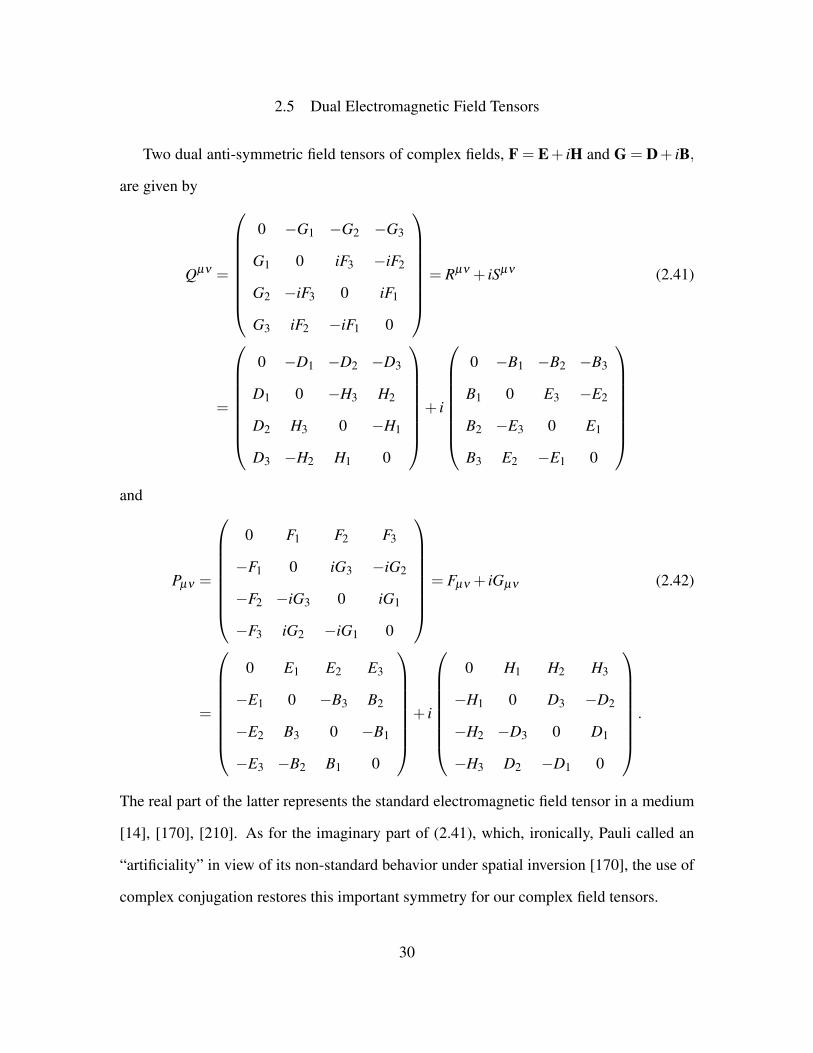
2.5 Dual Electromagnetic Field Tensors
Two dual anti-symmetric field tensors of complex fields, F = E+ iH and G = D+ iB,
are given by
Qµν =
0 −G1 −G2 −G3
G1 0 iF3 −iF2
G2 −iF3 0 iF1
G3 iF2 −iF1 0
= Rµν + iSµν (2.41)
=
0 −D1 −D2 −D3
D1 0 −H3 H2
D2 H3 0 −H1
D3 −H2 H1 0
+ i
0 −B1 −B2 −B3
B1 0 E3 −E2
B2 −E3 0 E1
B3 E2 −E1 0
and
Pµν =
0 F1 F2 F3
−F1 0 iG3 −iG2
−F2 −iG3 0 iG1
−F3 iG2 −iG1 0
= Fµν + iGµν (2.42)
=
0 E1 E2 E3
−E1 0 −B3 B2
−E2 B3 0 −B1
−E3 −B2 B1 0
+ i
0 H1 H2 H3
−H1 0 D3 −D2
−H2 −D3 0 D1
−H3 D2 −D1 0
.
The real part of the latter represents the standard electromagnetic field tensor in a medium
[14], [170], [210]. As for the imaginary part of (2.41), which, ironically, Pauli called an
“artificiality” in view of its non-standard behavior under spatial inversion [170], the use of
complex conjugation restores this important symmetry for our complex field tensors.
30
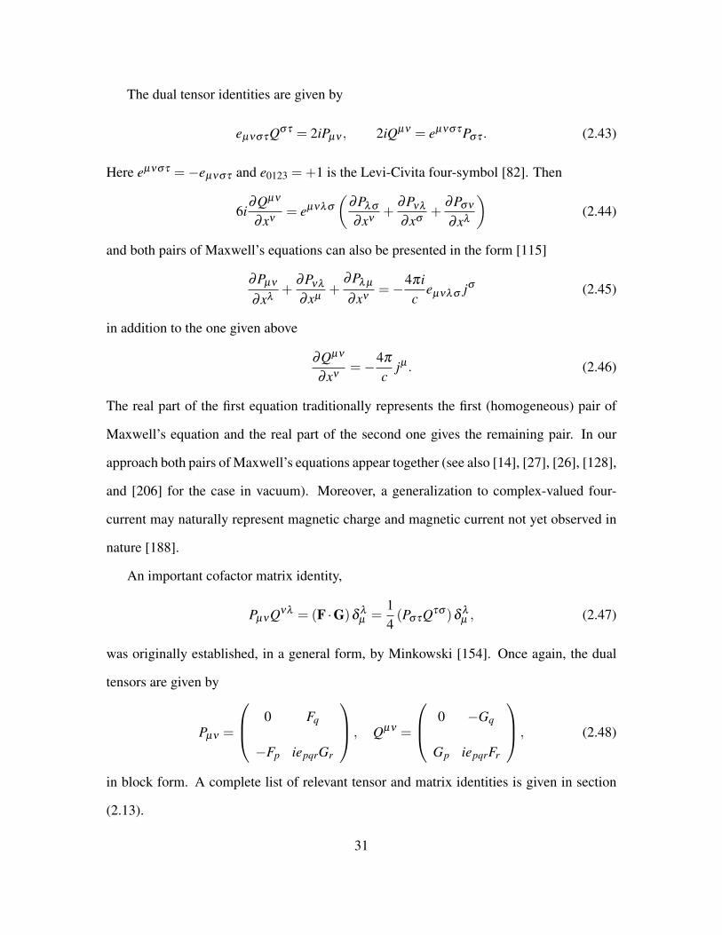
The dual tensor identities are given by
eµνστQστ = 2iPµν , 2iQµν = eµνστPστ . (2.43)
Here eµνστ =−eµνστ and e0123 =+1 is the Levi-Civita four-symbol [82]. Then
6i∂Qµν
∂xν= eµνλσ
(∂Pλσ
∂xν+
∂Pνλ
∂xσ+
∂Pσν
∂xλ
)(2.44)
and both pairs of Maxwell’s equations can also be presented in the form [115]
∂Pµν
∂xλ+
∂Pνλ
∂xµ+
∂Pλ µ
∂xν=−4πi
ceµνλσ jσ (2.45)
in addition to the one given above
∂Qµν
∂xν=−4π
cjµ . (2.46)
The real part of the first equation traditionally represents the first (homogeneous) pair of
Maxwell’s equation and the real part of the second one gives the remaining pair. In our
approach both pairs of Maxwell’s equations appear together (see also [14], [27], [26], [128],
and [206] for the case in vacuum). Moreover, a generalization to complex-valued four-
current may naturally represent magnetic charge and magnetic current not yet observed in
nature [188].
An important cofactor matrix identity,
PµνQνλ = (F ·G)δλµ =
14(PστQτσ )δ
λµ , (2.47)
was originally established, in a general form, by Minkowski [154]. Once again, the dual
tensors are given by
Pµν =
0 Fq
−Fp iepqrGr
, Qµν =
0 −Gq
Gp iepqrFr
, (2.48)
in block form. A complete list of relevant tensor and matrix identities is given in section
(2.13).
31
2.6 Covariant Derivation of Energy-Momentum Balance Equations
2.6.1 Preliminaries
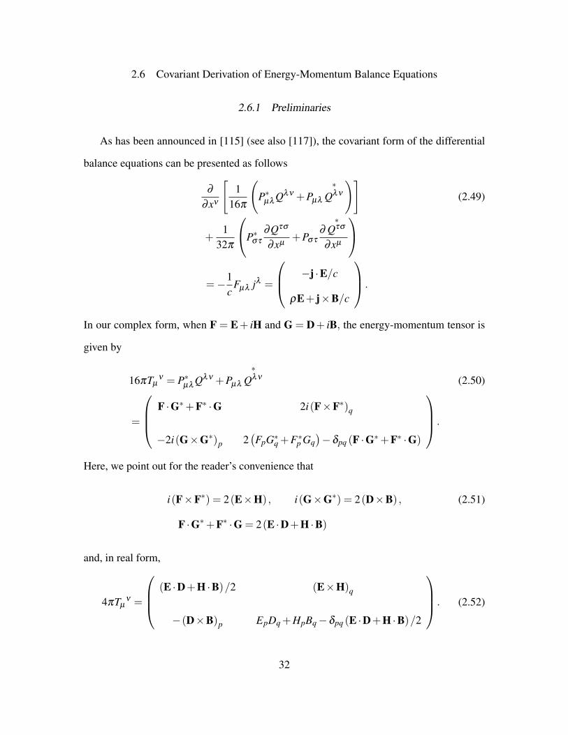
As has been announced in [115] (see also [117]), the covariant form of the differential
balance equations can be presented as follows
∂
∂xν
[1
16π
(P∗
µλQλν +Pµλ
∗Qλν
)](2.49)
+1
32π
P∗στ
∂Qτσ
∂xµ+Pστ
∂
∗Qτσ
∂xµ
=−1
cFµλ jλ =
−j ·E/c
ρE+ j×B/c
.
In our complex form, when F = E+ iH and G = D+ iB, the energy-momentum tensor is
given by
16πTµν = P∗
µλQλν +Pµλ
∗Qλν (2.50)
=
F ·G∗+F∗ ·G 2i(F×F∗)q
−2i(G×G∗)p 2(FpG∗q +F∗p Gq
)−δpq (F ·G∗+F∗ ·G)
.
Here, we point out for the reader’s convenience that
i(F×F∗) = 2(E×H) , i(G×G∗) = 2(D×B) , (2.51)
F ·G∗+F∗ ·G = 2(E ·D+H ·B)
and, in real form,
4πTµν =
(E ·D+H ·B)/2 (E×H)q
−(D×B)p EpDq +HpBq−δpq (E ·D+H ·B)/2
. (2.52)
32
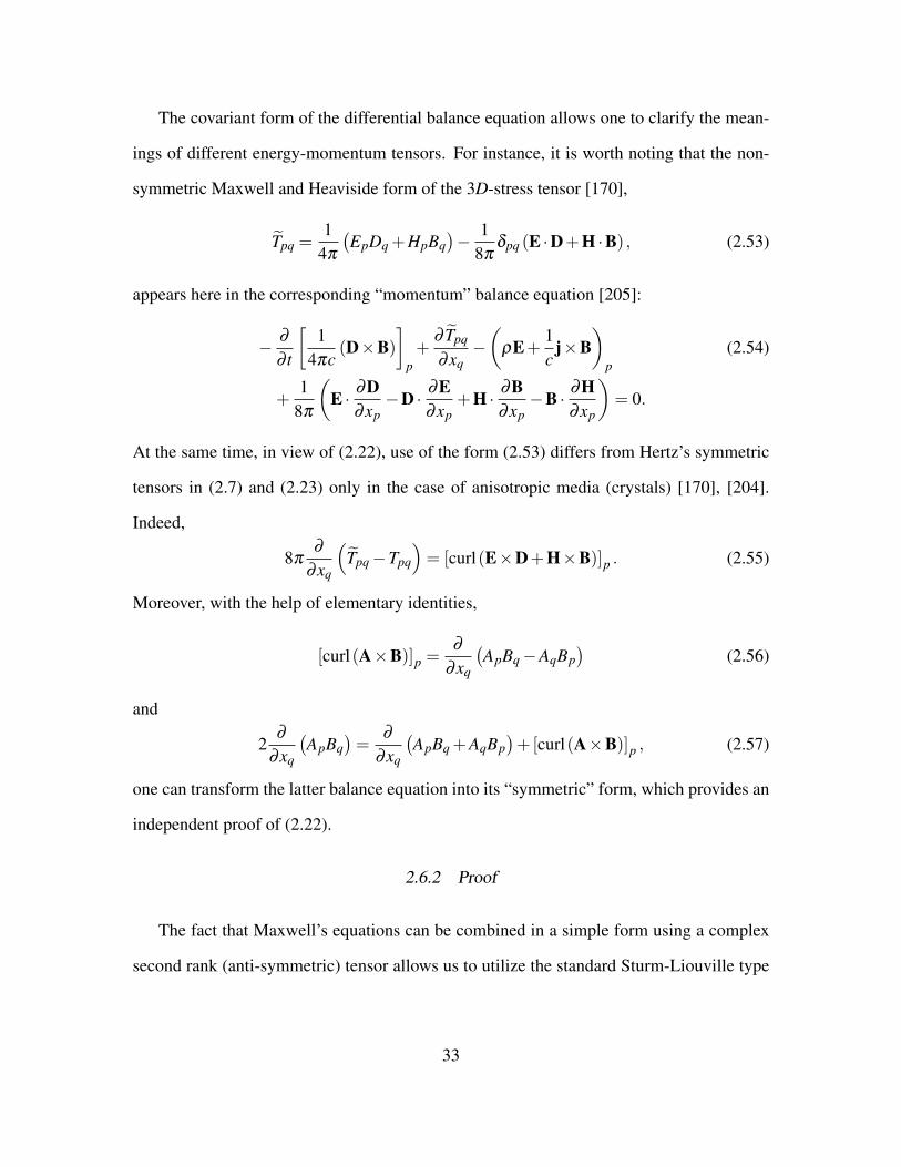
The covariant form of the differential balance equation allows one to clarify the mean-
ings of different energy-momentum tensors. For instance, it is worth noting that the non-
symmetric Maxwell and Heaviside form of the 3D-stress tensor [170],
Tpq =1
4π
(EpDq +HpBq
)− 1
8πδpq (E ·D+H ·B) , (2.53)
appears here in the corresponding “momentum” balance equation [205]:
− ∂
∂ t
[1
4πc(D×B)
]p+
∂ Tpq
∂xq−(
ρE+1c
j×B)
p(2.54)
+1
8π
(E · ∂D
∂xp−D · ∂E
∂xp+H · ∂B
∂xp−B · ∂H
∂xp
)= 0.
At the same time, in view of (2.22), use of the form (2.53) differs from Hertz’s symmetric
tensors in (2.7) and (2.23) only in the case of anisotropic media (crystals) [170], [204].
Indeed,
8π∂
∂xq
(Tpq−Tpq
)= [curl(E×D+H×B)]p . (2.55)
Moreover, with the help of elementary identities,
[curl(A×B)]p =∂
∂xq
(ApBq−AqBp
)(2.56)
and
2∂
∂xq
(ApBq
)=
∂
∂xq
(ApBq +AqBp
)+[curl(A×B)]p , (2.57)
one can transform the latter balance equation into its “symmetric” form, which provides an
independent proof of (2.22).
2.6.2 Proof
The fact that Maxwell’s equations can be combined in a simple form using a complex
second rank (anti-symmetric) tensor allows us to utilize the standard Sturm-Liouville type
33
argument in order to establish the energy-momentum differential balance equations in co-
variant form. Indeed, by adding matrix equation
P∗µλ
(∂Qλν
∂xν=−4π
cjλ
)(2.58)
and its complex conjugate
Pµλ
∂
∗Qλν
∂xν=−4π
cjλ
(2.59)
one gets
P∗µλ
∂Qλν
∂xν+Pµλ
∂
∗Qλν
∂xν=−8π
cFµλ jλ . (2.60)
A simple decomposition,
f∂g∂x
=12
∂
∂x( f g)+
12
(f
∂g∂x− ∂ f
∂xg)
(2.61)
with f = P∗µλ
and g = Qλν (and their complex conjugates), results in
∂
∂xν
[1
16π
(P∗
µλQλν +Pµλ
∗Qλν
)](2.62)
+1
16π
[(P∗
µλ
∂Qλν
∂xν−
∂Pµλ
∂xν
∗Qλν
)+(c.c.)
]=−1
cFµλ jλ .
By a direct substitution, one can verify that
Zµ = P∗µλ
∂Qλν
∂xν−
∂Pµλ
∂xν
∗Qλν =
12
P∗στ
∂Qτσ
∂xµ(2.63)
=−12
∗Qστ ∂Pτσ
∂xµ= F∗ · ∂G
∂xµ−G∗ · ∂F
∂xµ.
(An independent covariant proof of these identities is given in section (2.14)) Finally, in-
troducing
16πXµ = Zµ +Z∗µ , (2.64)
we obtain (2.49) with the explicitly covariant expression for the ponderomotive force (2.25),
which completes the proof.
34
As a result, the covariant energy-momentum balance equation is given by
∂
∂xνTµ
ν +Xµ =−1c
Fµλ jλ , (2.65)
in a compact form. If these differential equations are written for a stationary medium,
then the corresponding equations for moving bodies are uniquely determined, since the
components of a tensor in any inertial coordinate system can be derived by a proper Lorentz
transformation [170].
2.7 Covariant Derivation of Angular Momentum Balance
By definition, xµ = gµνxν =(ct,−r) and Tµλ =Tµνgνλ , where gµν =diag(1,−1,−1,−1)
= ∂xµ/∂xν . In view of (2.65), we derive
∂
∂xν
(xλ Tµ
ν − xµTλν)=(Tµλ −Tλ µ
)(2.66)
−(xλ Xµ − xµXλ
)− 1
c
(xλ Fµν − xµFλν
)jν
as a required differential balance equation.
With the help of familiar dual relations (2.127), one can get another covariant form of
the angular momentum balance equation:
∂
∂xν
(eµλστxσ Tτ
ν
)+ eµλστTστ (2.67)
+ eµλστxσ Xτ +1c
eµλστxσ Fτν jν = 0µλ .
In 3D-form, the latter relation can be reduced to (2.28)–(2.30).
Indeed, when µ = 0 and λ = p = 1,2,3, one gets
− 14πc
∂
∂ t
[epqrxq (D×B)r
]+
∂
∂xs
(epqrxqTrs
)(2.68)
+ epqrTqr + epqrxq (Xr +Yr) = 0,
where−Y= ρE+j×B/c is the familiar Lorentz force. Substitution, Trs =Trs+(
Trs−Trs
),
results in (2.28) in view of identity (2.55). The remaining cases, when µ,ν = p,q = 1,2,3,
35
can be analyzed in a similar fashion. In 3D-form, the corresponding equations can be
reduced to (2.21) and (2.54). Details are left to the reader.
Thus the angular momentum law has the form of a local balance equation, not a con-
servation law, since in general the energy-momentum tensor will not be symmetric [47].
Due to the asymmetry of this energy-momentum tensor a torque, for instance, may occur,
which cannot be compensated for by a change in the electromagnetic angular momentum.
Although this result may perhaps seem peculiar it is not in contradiction with experiment
according to [170].
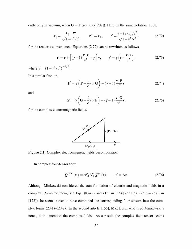
2.8 Transformation Laws of Complex Electromagnetic Fields
Let v be a constant real velocity vector representing uniform motion of one frame of
reference with respect to another one. Let us consider the following orthogonal decompo-
sitions,
F = F‖+F⊥, G = G‖+G⊥, (2.69)
such that our complex vectors
F‖,G‖
are collinear with the velocity vector v and F⊥,G⊥
are perpendicular to it (Figure 1). The Lorentz transformation of electric and magnetic
fields E,D,H,B take the following complex form
F′‖ = F‖, G′‖ = G‖ (2.70)
and
F′⊥ =F⊥−
ic(v×G)√
1− v2/c2, G′⊥ =
G⊥−ic(v×F)√
1− v2/c2. (2.71)
Although this transformation was found by Lorentz, it was Minkowski who realized that
this is the law of transformation of the second rank anti-symmetric four-tensors [138],
[154]; a brief historical overview is given in [170].) This complex 3D-form of the Lorentz
transformation of electric and magnetic fields was known to Minkowski (1908), but appar-
36
ently only in vacuum, when G = F (see also [207]). Here, in the same notation [170],
r′‖ =r‖−vt√1− v2/c2
, r′⊥ = r⊥, t ′ =t− (v · r)/c2√
1− v2/c2, (2.72)
for the reader’s convenience. Equations (2.72) can be rewritten as follows
r′ = r+[(γ−1)
v · rv2 − γt
]v, t ′ = γ
(t− v · r
c2
), (2.73)
where γ =(1− v2/c2)−1/2
.
In a similar fashion,
F′ = γ
(F− i
cv×G
)− (γ−1)
v ·Fv2 v (2.74)
and
G′ = γ
(G− i
cv×F
)− (γ−1)
v ·Gv2 v, (2.75)
for the complex electromagnetic fields.
Figure 2.1: Complex electromagnetic fields decomposition.
In complex four-tensor form,
Q′ µν (x′)= Λµ
σ ΛντQστ (x) , x′ = Λx. (2.76)
Although Minkowski considered the transformation of electric and magnetic fields in a
complex 3D-vector form, see Eqs. (8)–(9) and (15) in [154] (or Eqs. (25.5)–(25.6) in
[122]), he seems never to have combined the corresponding four-tensors into the com-
plex forms (2.41)–(2.42). In the second article [155], Max Born, who used Minkowski’s
notes, didn’t mention the complex fields. As a result, the complex field tensor seems
37

only to have appeared, for the first time, in [128] (see also [206]). The complex identity,
F ·G = invariant under the similarity transformation, follows from Minkowski’s determi-
nant relations (2.146)–(2.148).
Figure 2.2: Example of moving frame velocity.
Example. Let ek3k=1 be an orthonormal basis in R3 . We choose v = ve1 and write
x′µ = Λµ
νxν with
Λµ
ν =
γ −βγ 0 0
−βγ γ 0 0
0 0 1 0
0 0 0 1
, β =
vc, γ =
1√1−β 2
(2.77)
for the corresponding Lorentz boost (Figure 2). In view of (2.76), by matrix multiplication
38
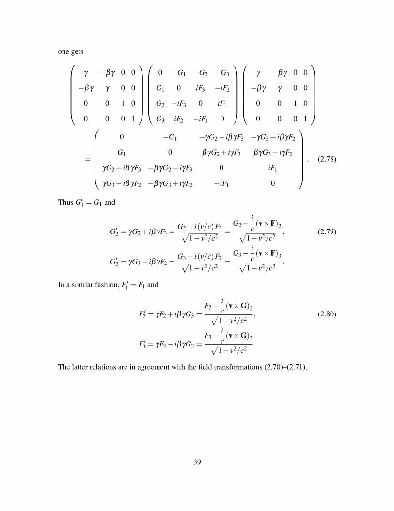
one gets
γ −βγ 0 0
−βγ γ 0 0
0 0 1 0
0 0 0 1
0 −G1 −G2 −G3
G1 0 iF3 −iF2
G2 −iF3 0 iF1
G3 iF2 −iF1 0
γ −βγ 0 0
−βγ γ 0 0
0 0 1 0
0 0 0 1
=
0 −G1 −γG2− iβγF3 −γG3 + iβγF2
G1 0 βγG2 + iγF3 βγG3− iγF2
γG2 + iβγF3 −βγG2− iγF3 0 iF1
γG3− iβγF2 −βγG3 + iγF2 −iF1 0
. (2.78)
Thus G′1 = G1 and
G′2 = γG2 + iβγF3 =G2 + i(v/c)F3√
1− v2/c2=
G2−ic(v×F)2√
1− v2/c2, (2.79)
G′3 = γG3− iβγF2 =G3− i(v/c)F2√
1− v2/c2=
G3−ic(v×F)3√
1− v2/c2.
In a similar fashion, F ′1 = F1 and
F ′2 = γF2 + iβγG3 =F2−
ic(v×G)2√
1− v2/c2, (2.80)
F ′3 = γF3− iβγG2 =F3−
ic(v×G)3√
1− v2/c2.
The latter relations are in agreement with the field transformations (2.70)–(2.71).
39
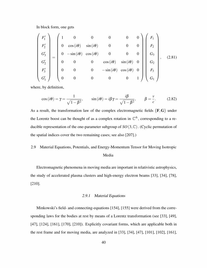
In block form, one gets
F ′1
F ′2
G′3
G′2
F ′3
G′1
=
1 0 0 0 0 0
0 cos(iθ) sin(iθ) 0 0 0
0 −sin(iθ) cos(iθ) 0 0 0
0 0 0 cos(iθ) sin(iθ) 0
0 0 0 −sin(iθ) cos(iθ) 0
0 0 0 0 0 1
F1
F2
G3
G2
F3
G1
, (2.81)
where, by definition,
cos(iθ) = γ =1√
1−β 2, sin(iθ) = iβγ =
iβ√1−β 2
, β =vc. (2.82)
As a result, the transformation law of the complex electromagnetic fields F,G under
the Lorentz boost can be thought of as a complex rotation in C6 , corresponding to a re-
ducible representation of the one-parameter subgroup of SO(3,C) . (Cyclic permutation of
the spatial indices cover the two remaining cases; see also [207].)
2.9 Material Equations, Potentials, and Energy-Momentum Tensor for Moving Isotropic
Media
Electromagnetic phenomena in moving media are important in relativistic astrophysics,
the study of accelerated plasma clusters and high-energy electron beams [33], [34], [78],
[210].
2.9.1 Material Equations
Minkowski’s field- and connecting-equations [154], [155] were derived from the corre-
sponding laws for the bodies at rest by means of a Lorentz transformation (see [33], [49],
[47], [124], [161], [170], [210]). Explicitly covariant forms, which are applicable both in
the rest frame and for moving media, are analyzed in [33], [34], [47], [101], [102], [161],
40

[166], [170], [182], [183], [207], [210] (see also the references therein). In standard nota-
tion,
β = v/c, γ =(1−β
2)−1/2, v = |v| , κ = εµ−1, (2.83)
one can write [33], [34], [49], [210]:
D = εE+κγ2
µ
[β
2E− vc2 (v ·E)+
1c(v×B)
], (2.84)
H =1µ
B+κγ2
µ
[−β
2B+vc2 (v ·B)+
1c(v×E)
].
In covariant form, these relations are given by
Rλν = ελνστFστ =
12
(ε
λνστ − ελντσ
)Fστ (2.85)
=14
(ε
λνστ − ελντσ + ε
νλτσ − ενλστ
)Fστ
(see [32], [33], [34], [101], [102], [182], [183], [210] and the references therein). Here,
ελνστ =
1µ
(gλσ +κuλ uσ
)(gντ +κuνuτ) = ε
νλτσ (2.86)
is the four-tensor of electric and magnetic permeabilities and
uλ = (γ,γv/c) , uλ uλ = 1 (2.87)
is the four-velocity of the medium ([182], [183], a computer algebra verification of these
relations is given in [127]). In a complex covariant form,(Qµν +
∗Qµν
)= ε
µνστ
(Pστ +
∗Pστ
). (2.88)
In view of (2.85) and (2.128)–(2.129), we get
Qµν =
(ε
µνστ − i2
eµνστ
)Fστ , Pµν =
(δ
λµ δ
ρ
ν −i2
eµνστεστλρ
)Fλρ , (2.89)
in terms of the real-valued electromagnetic field tensor.
41

2.9.2 Potentials
In practice, one can choose
Fστ =∂Aτ
∂xσ− ∂Aσ
∂xτ, (2.90)
for the real-valued four-vector potential Aλ (x) . Then
∂νQλν = ελνστ
∂ν (∂σ Aτ −∂τAσ )−i2
eλνστ∂ν (∂σ Aτ −∂τAσ )
=1µ
(gλσ +κuλ uσ
)(gντ +κuνuτ)∂ν (∂σ Aτ −∂τAσ )
by (2.86). Substitution into Maxwell’s equations (2.46) or (2.45) results in(gλσ +κuλ uσ
)−[∂
τ∂τ +κ (uτ
∂τ)2]
Aσ (2.91)
+∂σ (∂ τAτ +κuνuτ∂νAτ) =−
4πµ
cjλ ,
where −∂ τ∂τ = −gστ∂σ ∂τ = ∆− (∂/c∂ t)2 is the D’Alembert operator. In view of an
inverse matrix identity,(gλρ −
κ
1+κuλ uρ
)(gλσ +κuλ uσ
)= δ
σρ , (2.92)
the latter equations take the form2
[∂
τ∂τ +κ (uτ
∂τ)2]
Aσ −∂σ (∂ τAτ +κuνuτ∂νAτ) (2.93)
=4πµ
c
(gσλ −
κ
1+κuσ uλ
)jλ .
Subject to the subsidiary condition,
∂τAτ +κuνuτ
∂νAτ = (gντ +κuνuτ)∂νAτ = 0, (2.94)
these equations were studied in detail for the sake of development of the phenomenological
classical and quantum electrodynamics in a moving medium (see [31], [32], [33], [34],2Equations (2.90) and (2.93), together with the gauge condition (2.94), may be considered as the funda-
mentals of the theory [101]. Our complex fields are given by (2.89).
42
[166], [182], [177], [183], [210] and the references therein). In particular, Green’s functions
of the photon in a moving medium was studied in [101], [182], [177] (with applications to
quantum electrodynamics).
2.9.3 Hertz’s Tensor and Vectors
We follow [33], [34], [210] with somewhat different details. The substitution,
Aµ (x) =(
κ
1+κuµuλ −δ
µ
λ
)∂σ Zλσ (x) (2.95)
(a generalization of Hertz’s potentials for a moving medium [33], [210]), into the gauge
condition (2.94) results in Zλσ =−Zσλ , in view of(gνµ +κuνuµ
)∂
νAµ
=(gνµ +κuνuµ
)( κ
1+κuµuλ −δ
µ
λ
)∂
ν∂σ Zλσ
=−gνλ ∂ν∂σ Zλσ =−∂λ ∂σ Zλσ ≡ 0.
Then, equations (2.93) take the form[∂
τ∂τ +κ (uτ
∂τ)2]
∂σ Zλσ =−4πµ
cjλ . (2.96)
Indeed, the right-hand side of (2.93) is given by[∂
τ∂τ +κ (uτ
∂τ)2]
Aσ =[∂
τ∂τ +κ (uτ
∂τ)2]
gσ µAµ
=[∂
τ∂τ +κ (uτ
∂τ)2]
gσ µ
(κ
1+κuµuλ −δ
µ
λ
)∂σ Zλσ
=[∂
τ∂τ +κ (uτ
∂τ)2](
κ
1+κuσ uλ −gσλ
)∂σ Zλσ
=4πµ
c
(gσλ −
κ
1+κuσ uλ
)jλ
and the matrix is invertible.
Finally, with the help of the standard substitution,
jλ = c∂σ pλσ , pλσ =−pσλ (2.97)
43
(in view of ∂λ jλ = c∂λ ∂σ pλσ ≡ 0), we arrive at[∂
τ∂τ +κ (uτ
∂τ)2]
Zλν =−4π pλν . (2.98)
Here, by definition,
pλν =
0 p1 p2 p3
−p1 0 −m3 m2
−p2 m3 0 −m1
−p3 −m2 m1 0
(2.99)
is an anti-symmetric four-tensor [33], [34], [210]. The “electric” and “magnetic” Hertz
vectors, Z(e) and Z(m), are also introduced in terms of a single four-tensor,
Zλν =
0 Z(e)1 Z(e)
2 Z(e)3
−Z(e)1 0 −Z(m)
3 Z(m)2
−Z(e)2 Z(m)
3 0 −Z(m)1
−Z(e)3 −Z(m)
2 Z(m)1 0
. (2.100)
In view of (2.95), for the four-vector potential, Aλ = (ϕ,A) , we obtain
ϕ =−(
1− κγ2
1+κ
)∇ ·Z(e)+
κγ2
(1+κ)cv ·
(∂Z(e)
c∂ t+∇×Z(m)
)(2.101)
and
A =∂Z(e)
c∂ t+∇×Z(m) (2.102)
+κγ2v
(1+κ)c2
[c∇ ·Z(e)+
∂
c∂ t
(v ·Z(e)
)+v ·
(∇×Z(m)
)].
Then, equations (2.98) take the form[∂
τ∂τ +κ (uτ
∂τ)2]
Z(e) =−4πµp,[∂
τ∂τ +κ (uτ
∂τ)2]
Z(m) =−4πµm (2.103)
and, for the four-current, jλ = (cρ, j) , one gets
ρ =−∇ ·p, j =∂p∂ t
+ c∇×m (2.104)
44

(see [33], [34], [210] for more details).
The Hertz vector and tensor potentials, for a moving medium and at rest, were utilized
in [33], [34], [67], [81], [106], [205], [210], [218] (see also the references therein). Many
classical problems of radiation and propagation can be consistently solved by using these
potentials.
2.9.4 Energy-Momentum Tensor
In the case of the covariant version of the energy-momentum tensor given by (2.50),
the differential balance equations under consideration are independent of the particular
choice of the frame of reference. Therefore, our relations (2.89) are useful for derivation of
the expressions for the energy-momentum tensor and the ponderomotive force for moving
bodies from those for bodies at rest which were extensively studied in the literature. For
example, one gets
4πTµν = Fµλ ε
λνστFστ +14
δνµ Fστε
στλρFλρ (2.105)
with the help of (2.85) and (2.137).
2.10 Real vs Complex Lagrangians
In modern presentations of the classical and quantum field theories, the Lagrangian
approach is usually utilized.
45
2.10.1 Complex Forms
We introduce two quadratic “Lagrangian” densities
L0 = L ∗0 =
12
(PστQτσ +P∗στ
∗Qτσ
)(2.106)
=i4
eστκρ
(PστPκρ −P∗στP∗κρ
)= FστRτσ −GστSτσ = 2FστRτσ
= 4(E ·D−H ·B)
and
L1 =−L ∗1 = P∗στQτσ =
12
(P∗στQτσ −Pστ
∗Qτσ
)(2.107)
=i2
eστκρPστP∗κρ = 4i(E ·B−H ·D) .
Then, by formal differentiation,
∂L0
∂Pαβ
= Qβα ,∂L0
∂P∗αβ
=∗
Qβα (2.108)
and∂L1
∂P∗αβ
= Qβα ,∂L ∗
1∂Pαβ
=∗
Qβα (2.109)
in view of (2.130).
The complex covariant Maxwell equations (2.33) take the forms
∂
∂xν
(∂L0
∂Pνµ
)=−4π
cjµ ,
∂
∂xν
(∂L1
∂Pνµ
)=
4π
cjµ (2.110)
and the covariant energy-momentum balance relations (2.49) are given by
∂
∂xν
[1
16π
(P∗
µλ
∂L0
∂Pνλ
+Pµλ
∂L0
∂P∗νλ
)](2.111)
+1
32π
[P∗στ
∂
∂xµ
(∂L0
∂Pστ
)+Pστ
∂
∂xµ
(∂L0
∂P∗στ
)]=−1
cFµλ jλ
46
and
∂
∂xν
[1
16π
(Pµλ
∂L1
∂Pνλ
+P∗µλ
∂L ∗1
∂Pνλ
)](2.112)
+1
32π
[Pστ
∂
∂xµ
(∂L1
∂Pστ
)+P∗στ
∂
∂xµ
(∂L ∗
1∂P∗στ
)]=
1c
Fµλ jλ
in terms of the complex Lagrangians under consideration, respectively.
Finally, with the help of the following densities,
L0 = L0−4π
cjνAν , L1 = L1 +
4π
cjνAν , (2.113)
one can derive analogs of the Euler-Lagrange equations for electromagnetic fields in media:
∂
∂xν
(∂L0,1
∂Pνµ
)−
∂L0,1
∂Aµ
= 0. (2.114)
In the case of a moving isotropic medium, a relation between Pνµ and Aµ is given by our
equations (2.89)–(2.90).
2.10.2 Real Form
Taking the real and imaginary parts, Maxwell’s equations (2.46) can be written as fol-
lows
∂νRµν =−4π
cjµ , ∂νSµν = 0. (2.115)
Here,
−6∂νSµν = eµνλσ (∂νFλσ +∂σ Fνλ +∂λ Fσν)≡ 0,
with the help of (2.44) and (2.90). Thus the second set of equations is automatically satis-
fied when we introduce the four-vector potential. For the inhomogeneous pair of Maxwell’s
equations, the Lagrangian density is given by
L =14
FστRτσ − 4π
cjσ Aσ (2.116)
=14
FστετσλρFλρ −
4π
cjσ Aσ ,
47

in view of (2.85). Then, for “conjugate momenta” to the four-potential field Aµ , one gets
∂L∂(∂νAµ
) = ∂L∂Fστ
∂Fστ
∂(∂νAµ
) = Rµν (2.117)
and the corresponding Euler-Lagrange equations take a familiar form
∂ν
(∂L
∂(∂νAµ
))− ∂L∂Aµ
= 0. (2.118)
The latter equation can also be derived with the help of the least action principle [170],
[207], [209]. The corresponding Hamiltonian and quantization are discussed in [94], [101],
[182] among other classical accounts.
In conclusion, it is worth noting the role of complex fields in quantum electrodynam-
ics, quadratic invariants and quantization (see, for instance, [4], [27], [26], [54], [101],
[102], [110], [114], [182], [177], [183], [209], [223]). The classical and quantum theory of
Cherenkov radiation is reviewed in [5], [30], [31], [87], [204]. For paraxial approximation
in optics, see [81], [112], [143], [142] and the references therein. Maxwell’s equations in
the gravitational field are discussed in [36] [82]. One may hope that our detailed mathe-
matical consideration of several aspects of macroscopic electrodynamics will be useful for
future investigations and pedagogy.
2.11 Formulas from Vector Calculus
Among useful differential relations are
∇ · (A×B) = B · (∇×A)−A · (∇×B) . (2.119)
∇ · ( f A) = (∇ f ) ·A+ f (∇ ·A) . (2.120)
∇× ( f A) = (∇ f )×A+ f (∇×A) . (2.121)
A · (∇× ( f ∇×B))−B · (∇× ( f ∇×A)) (2.122)
= ∇ · ( f (B× (∇×A)−A× (∇×B))) .
48
A(∇ ·B)−B(∇ ·A)+A× (∇×B)−B× (∇×A) (2.123)
−∇× (A×B) =3
∑α=1
A2α∇
(Bα
Aα
)=−
3
∑α=1
B2α∇
(Aα
Bα
).
(See also [3], [188] and [209].)
2.12 Dual Tensor Identities
In this chapter, eµνστ = −eµνστ and e0123 = +1 is the Levi-Civita four-symbol [82]
with familiar contractions:
eµνστeµκλρ =−
∣∣∣∣∣∣∣∣∣∣δ ν
κ δ ν
λδ ν
ρ
δ σκ δ σ
λδ σ
ρ
δ τκ δ τ
λδ τ
ρ
∣∣∣∣∣∣∣∣∣∣, (2.124)
eµνστeµνλρ =−2
∣∣∣∣∣∣∣δ σ
λδ σ
ρ
δ τ
λδ τ
ρ
∣∣∣∣∣∣∣=−2(
δσ
λδ
τρ −δ
σρ δ
τ
λ
), (2.125)
eµνστeµνσρ =−6δτρ , eµνστeµνσρ =−24. (2.126)
Dual second rank four-tensor identities are given by [82]:
eµνστAστ = 2Bµν , eµνστBστ = Aνµ −Aµν . (2.127)
In particular,
Qµν = Rµν + iSµν = Rµν − i2
eµνστFστ , (2.128)
Pµν = Fµν + iGµν = Fµν −i2
eµνστRστ . (2.129)
eµνστQστ = 2iPµν , 2iQµν = eµνστPστ . (2.130)
2Rµν = eµνστGστ , −2Sµν = eµνστFστ . (2.131)
2Gµν =−eµνστRστ , 2Fµν = eµνστSστ . (2.132)
49
PµνQµν = 2FµνRµν − i2(eµνστFµνFστ + eµνστRµνRστ
). (2.133)
By direct calculation,
FµνRµν = 2(H ·B−E ·D) , (2.134)
eµνστFµνFστ = 8E ·B, eµνστRµνRστ = 8H ·D. (2.135)
As a result,14
PµνQµν = H ·B−E ·D− i(E ·B+H ·D) . (2.136)
An important decomposition,
P∗µλ
Qλν +Pµλ
∗Qλν = 2
(Fµλ Rλν +Gµλ Sλν
)(2.137)
= 4Fµλ Rλν +δνµ FστRστ
= 4Fµλ Rλν −2δνµ (E ·D−H ·B) ,
is complemented by an identity,
Pµλ Qλν +P∗µλ
∗Qλν =
14
(PστQτσ +P∗στ
∗Qτσ
)δ
νµ (2.138)
=12(E ·D−H ·B)δ
νµ .
In matrix form,
PQ = (F + iG)(R+ iS) = (FR−GS)+ i(FS+GR) , (2.139)
P∗Q = (F− iG)(R+ iS) = (FR+GS)+ i(FS−GR) . (2.140)
Here,
FS =14
Tr(FS) I = (E ·B) I, (2.141)
GR =14
Tr(GR) I = (H ·D) I. (2.142)
FR−GS =12
Tr(FR) I = (E ·D−H ·B) I, (2.143)
50

FR+GS = 2FR− 12
Tr(FR) I (2.144)
= 2FR− (E ·D−H ·B) I.
Tr(FR+GS) = 0, (2.145)
where I =diag(1,1,1,1) is the identity matrix.
Also,
PQ = QP = (F ·G) I, (2.146)
detP = detQ =−(F ·G)2 (2.147)
and
F ·G = (E+ iH) · (D+ iB) (2.148)
= (E ·D−H ·B)+ i(E ·B+H ·D) .
Other useful dual four-tensor identities are given by [82]:
eµνστAνστ = 6Bµ , Aµνλ = eµνλσ Bσ . (2.149)
In particular,
6i∂Qµν
∂xν= eµνλσ
(∂Pλσ
∂xν+
∂Pνλ
∂xσ+
∂Pσν
∂xλ
), (2.150)
and∂Pµν
∂xλ+
∂Pνλ
∂xµ+
∂Pλ µ
∂xν= ieµνλσ
∂Qστ
∂xτ(2.151)
(see also [115]).
2.13 Proof of Identities (2.63)
In view of (2.43), or (2.130), and (2.151), we can write(∂Pµν
∂xλ+
∂Pνλ
∂xµ+
∂Pλ µ
∂xν= ieµνλσ
∂Qστ
∂xτ
) ∗Qλν , (2.152)
51

or
2∗
Qλν∂Pµν
∂xλ+
∗Qλν ∂Pνλ
∂xµ
= i
(eµνλσ
∗Qλν
)∂Qστ
∂xτ=−2P∗µσ
∂Qστ
∂xτ
by (2.130). Therefore,
P∗µλ
∂Qλν
∂xν−
∂Pµλ
∂xν
∗Qλν =−1
2
∗Qστ ∂Pτσ
∂xµ. (2.153)
In addition, with the help of (2.130) one gets
2i(
P∗στ
∂Qτσ
∂xµ
)= P∗στeτσλν ∂Pλν
∂xµ
= eστνλ P∗στ
∂Pλν
∂xµ=−2i
( ∗Qστ ∂Pτσ
∂xµ
),
which completes the proof.
52
Chapter 3
THE PAULI-LUBANSKI VECTOR AND PHOTON HELICITY
In this chapter, a classical concept of photon helicity is investigated from the viewpoint
of the Pauli-Lubanski vector. This problem is considered from first principles of the repre-
sentation theory of the Poincare group. In particular, a misconception in the definition of
helicity for a massless particle, in which a linear relation, w = λ p, is used in standard quan-
tum field theory textbooks is discovered. In addition, as a result, this analysis also leads to
a new approach, introduced here, for the derivation of Maxwell’s equations in vacuum. All
physically interesting unitary ray representations of the proper orthochronous inhomoge-
neous Lorentz group (known nowadays as the Poincare group) were classified by Wigner
[231] and, since then, this approach has been utilized for the mathematical description of
mass and spin of an elementary particle. By definition, the Pauli-Lubanski pseudo-vector1
is given by
wµ =12
eµνστ pνMστ , pµwµ = 0, (3.1)
where pµ is the relativistic linear momentum operator and Mστ are the corresponding an-
gular momentum operators. The mass and spin of a particle are defined in terms of two
quadratic invariants (Casimir operators of the Poincare group) as follows
p2 = pµ pµ = m2, w2 = wµwµ =−m2s(s+1) , m > 0 (3.2)
(see, for example, [11], [12], [29], [121], [133], [139], [140], [141], [181], [184], [185],
[187] and the references therein; we use the standard notations that were mentioned in the
introduction and are repeated here for convenience).1The pseudo-vector nature can be seen by the fact that w′µ = det(Λ)Λσ
µ wσ , which follows from
p′ν = Λνκ pκ , M′στ = Λσ
α Λτ
βMαβ , and the determinant identity det(Λ)eκγαβ = eµνστ Λ
µ
κ Λνγ Λσ
α Λτ
β.
53

For the massless fields, when m= 0, one gets w2 = p2 = pw= 0, and the Pauli-Lubanski
vector should be proportional to p : 2
wµ = λ pµ (3.3)
(acting on the corresponding eigenstates [160], [184]). The number λ is called the helicity
of the representation and the value s = |λ | is sometimes called the spin of a particle with
zero mass [29], [184], [185], [187]. One of the goals of this chapter is to show that, in the
case of the electromagnetic field, the sign of the constant λ in the latter equation is fixed
by the condition that the classical Maxwell equations hold.
As a result, instead of being given by the constant of proportionality in relation (3.3),
the helicity of the photon should be defined, as it is traditionally done in particle physics, by
λ = k ·M/k0, where k = (k0,k) and M is the photon angular momentum (k2 = k20−k2 = 0).
But one needs a proper realization of the action of these operators on the photon field tensor
in covariant form [154], [155]; or, in 3D-form, on the complex electromagnetic field vector
F = E+ iH discussed in [14], [16], [24], [26], [122], [128], [154], [181], [188], [191],
[192], [206], [224]. The sign of the constant λ = ±1 is fixed then by a “continuity”, in
view of the invariance of the upper(lower) light cone under a proper Lorentz transformation
(see, for example, [29], [121] and [212]).
3.1 Transformation Laws and Generators
Under the Lorentz transformation [29], [154], [157], [181],
U (Λ)Qµν (xρ) := Q′µν
(Λ
κρxρ
)= Λ
µ
σ Λντ Qστ (xρ) , (3.4)
2This assumption was made by Bargmann and Wigner [12] for the massless limit of the spinor wave
equation for particles with an arbitrary integer or half-integer spin proposed by Dirac [51] (see also [74],
[75], [113], [169], [48] and the references therein). The pseudo-vector (3.1) was introduced, in a slightly
different notation, by Eqs. (4.a)–(4.b) of Ref. [12].
54

where the summation is assumed over any two repeated indices3. We shall use the follow-
ing six 4×4 matrices (α,β = 0,1,2,3 are fixed):
Λ(θαβ
)= exp
(−θαβ mαβ
), mαβ =−mβα , (3.5)(
mαβ
)µ
ν= gαµ
δβ
ν −gβ µδ
αν .
for the corresponding one-parameter subgroups of the proper Lorentz group [29], [157],
[187] with the standard metric, gµν = gµν =diag(1,−1,−1,−1) , in the Minkowski space-
time. The 4-angular momentum operators,
Mαβ = xβ∂
α − xα∂
β , ∂α = gακ
∂κ , (3.6)
can be derived as follows
Mαβ Qµν :=−[
ddθαβ
Qµν
(Λ
κρ
(θαβ
)xρ
)]∣∣∣∣θαβ=0
(3.7)
=(
mαβ
)µ
σQσν +Qµτ
(mαβ
)ν
τ
with (mαβ
)µ
ν=−
dΛµ
ν
(θαβ
)dθαβ
∣∣∣∣∣θαβ=0
= gαµδ
β
ν −gβ µδ
αν . (3.8)
In matrix form,
Mαβ Q = mαβ Q+Q(
mαβ
)T, (3.9)
where Q = Qµν and mT is the transposed matrix. The latter equations (3.7), (3.8), and (3.9)
define the action of the infinitesimal operators on the complex field tensor,
MστQαβ = gσαQτβ −gταQσβ +gσβ Qατ −gτβ Qασ , (3.10)3Although Minkowski considered the transformation of electric and magnetic fields in a complex 3D
vector form, see Eqs. (8)–(9) and (15) in [154] (or Eqs. (25.5)–(25.6) in [122]), he seems never to have
combined the corresponding 4-tensors into the complex forms (2.41)–(2.42). In the second article [155],
Max Born, who used Minkowski’s notes, didn’t mention the complex fields. As a result, the complex field
tensor seems only to have appeared, for the first time, in [128] (see also [206]).
55

in the form that is required in equation (3.15) below.
In a similar fashion, for the products of the generators,
Mαβ Mγδ Qµν =(
mγδ
)µ
κ
(mαβ
)κ
σQσν +
(mαβ
)µ
σ
(mγδ
)ν
ρQσρ (3.11)
+(
mγδ
)µ
κ
(mαβ
)ν
τQκτ +
(mγδ
)ν
ρ
(mαβ
)ρ
τQµτ ,
or, in matrix form,
Mαβ Mγδ Q =(
mγδ mαβ
)Q−
((mγδ mαβ
)Q)T
(3.12)
+mαβ Q(
mγδ
)T−(
mαβ Q(
mγδ
)T)T
.
As a result, [Mαβ , Mγδ
]:= Mαβ Mγδ −Mγδ Mαβ (3.13)
= gαγMβδ −gαδ Mβγ +gβδ Mαγ −gβγMαδ ,
which follows from (3.7)–(3.8) and can be verified, once again, by using (3.6).
Finally, introducing the infinitesimal operators M =(M23,M31,M12) and
N =(M01,M02,M03) for the rotations and boosts, respectively, one can get
N2Q =−M2Q = 2Q, (M ·N)Q =−2iQ. (3.14)
The Casimir operators of the proper Lorentz group are given by (M+ iN)2 /4 = 0 and
(M−iN)2 /4 =−2 in the space of complex anti-symmetric tensors under consideration. In
view of M2 = −s(s+1) = −2, we may say that the spin of the photon is equal to one.
(Here, we have chosen real-valued generators; see also [10], [12], [85], [181], [187] and
[226] for more details on the Lorentz group representations.)
3.2 The Pauli-Lubanski Vector and Maxwell’s Equations in Vacuum
As follows from the representation theory of the Poincare group [12], [29] and the
geometry of the Minkowski space-time [156], [160], for the case of massless particles, the
56

Pauli-Lubanski vector should be collinear to the operator of the 4-linear momentum. For a
classical electromagnetic field, this relation takes the form
12
eµνστ∂ν
(MστQαβ
)=−i∂µQαβ , (3.15)
and by (3.10), we find that
gααeαµντ∂νQτβ −gββ eβ µντ∂
νQτα =−i∂µQαβ (3.16)
(α,β = 0,1,2,3 are fixed; no summation is assumed over these two indices). By a direct,
but rather tedious evaluation, one can verify that the latter equation, which is written in
terms of a third rank 4-tensor, is equivalent to the original system of Maxwell equations in
vacuum, ∂νQµν = 0. As a result, the helicity of the photon4, or a harmonic circular classical
electromagnetic wave, cannot be defined as an undetermined sign, or an extra ±1 factor, in
the right hand side of equation (3.15) as it is stated in standard textbooks on the quantum
field theory [12], [29], [184], [185], [187].
In view of (3.15), for the rotations and boosts, M =(M23,M31,M12) and
N =(M01,M02,M03) , respectively, the following standard equations hold
(∇ ·M)Q = i∂0Q, ∂0 =1c
∂
∂ t(3.17)
and
∂0MQ+(∇×N)Q = i∇Q, (3.18)
where Q = Qαβ =−Qβα is the complex field tensor and the actions of operators M and N
on this tensor are explicitly defined by (3.10).
Note. In vacuum, when G=F and ρ = 0, j= 0, two different covariant forms of Maxwell’s
equations are given by
∂νQµν = 0, ∂νPµν = 0, (3.19)
4Multiple meanings of the word “photon” are analyzed in [111].
57

where ∂ ν = gνµ∂µ = gνµ∂/∂xµ . The second equation follows from (3.16), when one takes
µ = β and sums over β = 0,1,2,3 with the help of (2.43). As another useful consequence
of our equation (3.16), one can directly show that the d’Alembert operator annihilates any
component of the complex field tensor in vacuum,
∂µ
∂µQαβ =
(1c2
∂ 2
∂ t2 −∆
)Qαβ =Qαβ = 0, (3.20)
thus de-coupling the system. It is worth noting that, in covariant form, our derivation does
not require any formula of 3D-vector calculus. (The general theory of relativistic-invariant
equations is studied in classical accounts [12], [22], [50], [51], [74], [75], [85], [113], [144],
[169], [176]; see also [27], [89], [139], [140], [141], [48] and the references therein.)
3.3 Examples
In a matrix form, equation (3.17) can be rewritten as follows
0 −∂2G3 +∂2G3 ∂1G3−∂3G1 −∂1G2 +∂2G1
∂2G3−∂2G3 0 i(∂1F2−∂2F1) i(∂1F3−∂3F1)
−∂1G3 +∂3G1 −i(∂1F2−∂2F1) 0 i(∂2F3−∂3F2)
∂1G2−∂2G1 −i(∂1F3−∂3F1) −i(∂2F3−∂3F2) 0
=+ic
∂
∂ t
0 −G1 −G2 −G3
G1 0 iF3 −iF2
G2 −iF3 0 iF1
G3 iF2 −iF1 0
, (3.21)
or 0 −(curlG)q
(curlG)p iepqr (curlF)r
=ic
∂
∂ t
0 −Gq
Gp iepqrFr
, (3.22)
58
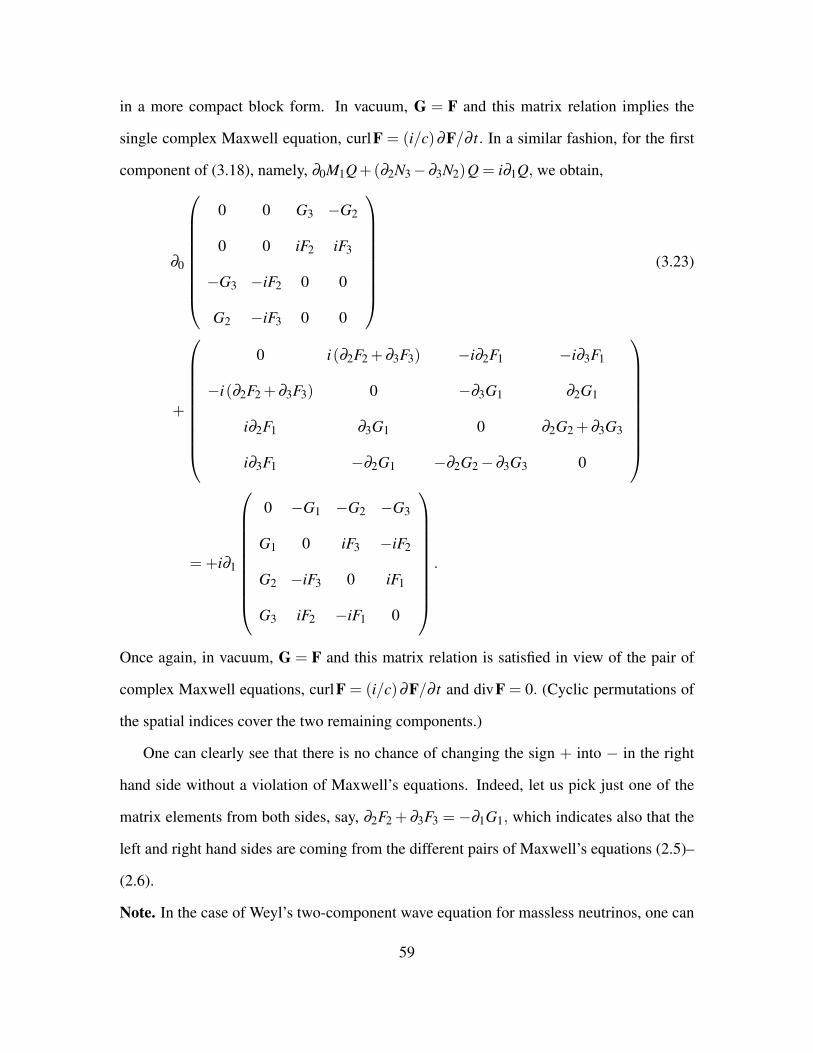
in a more compact block form. In vacuum, G = F and this matrix relation implies the
single complex Maxwell equation, curlF = (i/c)∂F/∂ t. In a similar fashion, for the first
component of (3.18), namely, ∂0M1Q+(∂2N3−∂3N2)Q = i∂1Q, we obtain,
∂0
0 0 G3 −G2
0 0 iF2 iF3
−G3 −iF2 0 0
G2 −iF3 0 0
(3.23)
+
0 i(∂2F2 +∂3F3) −i∂2F1 −i∂3F1
−i(∂2F2 +∂3F3) 0 −∂3G1 ∂2G1
i∂2F1 ∂3G1 0 ∂2G2 +∂3G3
i∂3F1 −∂2G1 −∂2G2−∂3G3 0
=+i∂1
0 −G1 −G2 −G3
G1 0 iF3 −iF2
G2 −iF3 0 iF1
G3 iF2 −iF1 0
.
Once again, in vacuum, G = F and this matrix relation is satisfied in view of the pair of
complex Maxwell equations, curlF = (i/c)∂F/∂ t and divF = 0. (Cyclic permutations of
the spatial indices cover the two remaining components.)
One can clearly see that there is no chance of changing the sign + into − in the right
hand side without a violation of Maxwell’s equations. Indeed, let us pick just one of the
matrix elements from both sides, say, ∂2F2 +∂3F3 = −∂1G1, which indicates also that the
left and right hand sides are coming from the different pairs of Maxwell’s equations (2.5)–
(2.6).
Note. In the case of Weyl’s two-component wave equation for massless neutrinos, one can
59
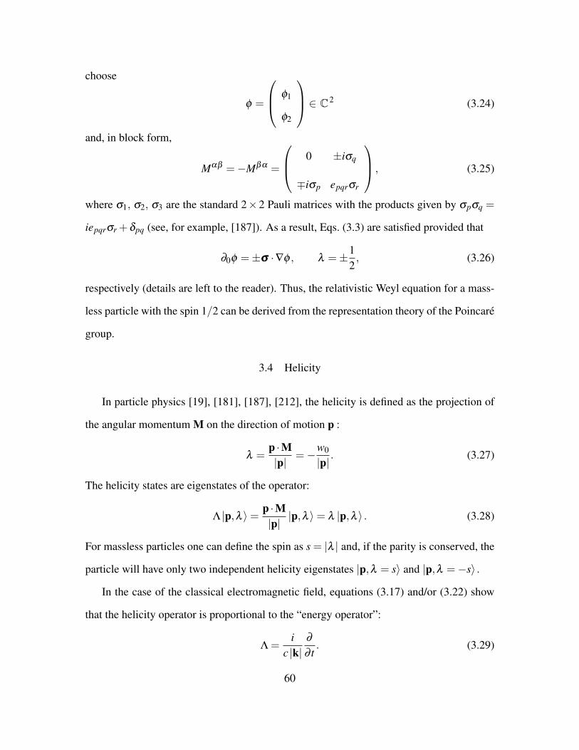
choose
φ =
φ1
φ2
∈ C2 (3.24)
and, in block form,
Mαβ =−Mβα =
0 ±iσq
∓iσp epqrσr
, (3.25)
where σ1, σ2, σ3 are the standard 2×2 Pauli matrices with the products given by σpσq =
iepqrσr +δpq (see, for example, [187]). As a result, Eqs. (3.3) are satisfied provided that
∂0φ =±σσσ ·∇φ , λ =±12, (3.26)
respectively (details are left to the reader). Thus, the relativistic Weyl equation for a mass-
less particle with the spin 1/2 can be derived from the representation theory of the Poincare
group.
3.4 Helicity
In particle physics [19], [181], [187], [212], the helicity is defined as the projection of
the angular momentum M on the direction of motion p :
λ =p ·M|p|
=−w0
|p|. (3.27)
The helicity states are eigenstates of the operator:
Λ |p,λ 〉= p ·M|p||p,λ 〉= λ |p,λ 〉 . (3.28)
For massless particles one can define the spin as s = |λ | and, if the parity is conserved, the
particle will have only two independent helicity eigenstates |p,λ = s〉 and |p,λ =−s〉 .
In the case of the classical electromagnetic field, equations (3.17) and/or (3.22) show
that the helicity operator is proportional to the “energy operator”:
Λ =i
c |k|∂
∂ t. (3.29)
60

As a result, these two operators have common eigenstates, |k,λ 〉 = Qµν , in the space of
complex anti-symmetric 4-tensors of the second rank. (The simplest covariant helicity
states will be constructed in the next section.)
On the other hand, in 3D-complex electrodynamics, one can take the complex vector
field |k,λ 〉= F = E+ iH and choose the following real-valued spin matrices [214]:
s1 =
0 0 0
0 0 −1
0 1 0
, s2 =
0 0 1
0 0 0
−1 0 0
, s3 =
0 −1 0
1 0 0
0 0 0
, (3.30)
such that[sp,sq
]= spsq− sqsp = epqrsr and s2
1 + s22 + s2
3 =−2. Then
(∇ · s)F := ∂1 (s1F)+∂2 (s2F)+∂3 (s3F) (3.31)
= ∂1
0 0 0
0 0 −1
0 1 0
F1
F2
F3
+∂2
0 0 1
0 0 0
−1 0 0
F1
F2
F3
+∂3
0 −1 0
1 0 0
0 0 0
F1
F2
F3
=
∂2F3−∂3F2
∂3F1−∂1F3
∂1F2−∂2F1
= curlF.
Once again, our representation (3.29) for the helicity operator holds in view of the Maxwell
equation in vacuum, curlF = (i/c)∂F/∂ t.
Note. In view of (3.29), the traditional definition of helicity (3.28) is related to separation
of variables in Maxwell’s equations. Letting Qµν = q(t)Zµν (r) , one gets
0 =∂Qµν
∂xν=
1c
∂Qµ0
∂ t+
∂Qµ p
∂xp=
1c·q(t)Zµ0 (r)+q(t)
∂Zµ p (r)∂xp
, (3.32)
or
−·qcq
Zµ0 =∂Zµ p
∂xp, q = e−iωt , (3.33)
61
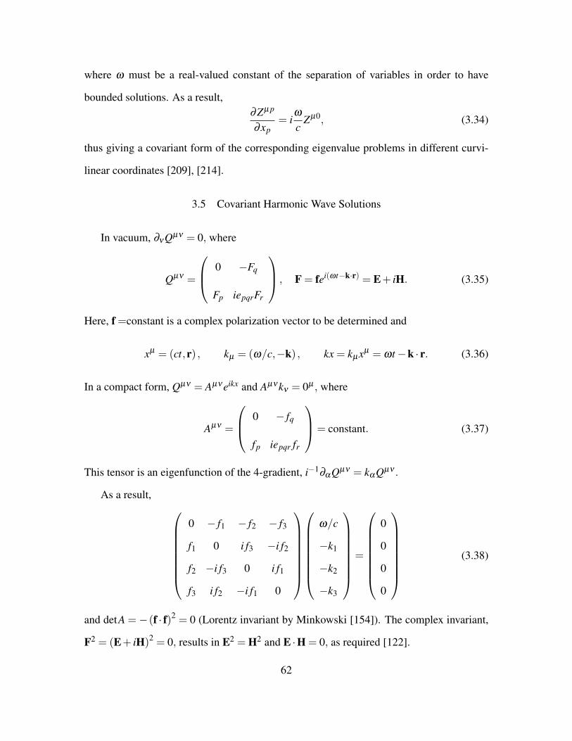
where ω must be a real-valued constant of the separation of variables in order to have
bounded solutions. As a result,∂Zµ p
∂xp= i
ω
cZµ0, (3.34)
thus giving a covariant form of the corresponding eigenvalue problems in different curvi-
linear coordinates [209], [214].
3.5 Covariant Harmonic Wave Solutions
In vacuum, ∂νQµν = 0, where
Qµν =
0 −Fq
Fp iepqrFr
, F = fei(ωt−k·r) = E+ iH. (3.35)
Here, f =constant is a complex polarization vector to be determined and
xµ = (ct,r) , kµ = (ω/c,−k) , kx = kµxµ = ωt−k · r. (3.36)
In a compact form, Qµν = Aµνeikx and Aµνkν = 0µ , where
Aµν =
0 − fq
fp iepqr fr
= constant. (3.37)
This tensor is an eigenfunction of the 4-gradient, i−1∂αQµν = kαQµν .
As a result,
0 − f1 − f2 − f3
f1 0 i f3 −i f2
f2 −i f3 0 i f1
f3 i f2 −i f1 0
ω/c
−k1
−k2
−k3
=
0
0
0
0
(3.38)
and detA =−(f · f)2 = 0 (Lorentz invariant by Minkowski [154]). The complex invariant,
F2 = (E+ iH)2 = 0, results in E2 = H2 and E ·H = 0, as required [122].
62

In 3D-form, the latter system of linear equations gives an eigenvalue problem:
ik× f =ω
cf, f · f = 0. (3.39)
The eigenvalues are∣∣∣∣∣∣∣∣∣∣−ω/c −ik3 ik2
ik3 −ω/c −ik1
−ik2 ik1 −ω/c
∣∣∣∣∣∣∣∣∣∣=
ω
c
(k2
1 + k22 + k2
3−ω2
c2
)= 0. (3.40)
The case ω = 0, when f = k, does not satisfy the second condition f2 = 0 unless k = 0.
Therefore, there are only two eigenvectors f, f∗, corresponding to ω/c = ±k =
±√
k21 + k2
2 + k23 :
f =k× (lll×k)+ ik (k× lll)
k√
2 |k× lll|, f∗ = f|k→−k , (3.41)
respectively [26]. Here, lll is an arbitrary real vector that is not collinear to k (k 6=constant lll)
and f · f∗ = 1. (A similar eigenvalue problem occurs in the mean magnetic field generation,
called αΩ-dynamo, in cosmic astrophysics [78].)
Example. Let ek3k=1 be an orthonormal basis in R3 . One can choose lll = e1 and k = ke3.
Then
f =e1 + ie2√
2, f∗ =
e1− ie2√2
(3.42)
(see [26], [122], and [209] for more details).
3.6 Discrete Transformations and Polarization
The complex Maxwell equations in vacuum,
ic
∂F∂ t
= curlF, divF = 0, (3.43)
are invariant under the following discrete transformations: spatial inversion P: F(r, t)→
F∗ (−r, t) ; time reversal T: F(r, t)→ F∗ (r,−t) ; and space-time inversion PT: F(r, t)→
63
F(−r,−t) . They, together with the identity transformation, correspond to the four con-
nected components of the Poincare group. These transformations form the so-called Klein
group Identity,P,T,PT , with the following Cayley table.
* I P T PT
I I P T PT
P P I PT T
T T TP I P
PT PT T P I
The action of this group generates the following four circularly polarized waves (ω =
+ck):
F1 = fei(k·r−ωt), F2 = f∗e−i(k·r+ωt) = F∗1|t→−t = TF1 (3.44)
and
F3 = fe−i(k·r−ωt) = F1|r→−r,t→−t = (PT)F1, (3.45)
F4 = f∗ei(k·r+ωt) = F∗3|t→−t = TF3 = PF1.
They represent right- and left-handed circularly polarized waves moving along the vector
k in opposite directions. One can easily verify that the solutions F1,F2 correspond to
λ =+1 and F3,F4 have λ =−1. Also, F1 ·F3 = f2 = 0 and F2 ·F4 =(f2)∗ = 0. These
four solutions are linearly independent.
Example. The standard circular, elliptic, and linear polarizations of the classical electro-
magnetic waves occur as a result of superposition of the complex solutions under consid-
eration. With the help of the polarization vectors (3.42), one gets
F = c1F1 +F3
2+ c2
F1−F3
2= E+ iH (3.46)
= c1e1 cos(k · r−ωt)− c2e2 sin(k · r−ωt)
+ i[c2e1 cos
(k · r−ωt− π
2
)− c1e2 sin
(k · r−ωt− π
2
)],
64
where c1 = c∗1 and c2 = c∗2. For the elliptic polarization, we choose |c1| > |c2| or |c1| <
|c2| ; the linear polarization arises, for instance, if c1 6= 0 and c2 = 0 (see [122] and [209],
problems 2.128–2.134, for more details).
In conclusion, it is worth noting that, here, we have only discussed the classical electro-
magnetic field in vacuum. Different aspects of the “photon paradigm” are emphasized in
[111]. The photon wave functions are dealt with in [6], [19], [23], [24], [57], [80], [187].
For quantization in the complex form, see [23], [25], [27], [26] and the references therein.
(General quantization procedures are discussed, for example, in [27], [29], [110], [114],
[118], [158], [159], [184], [185], [187], [189], [209].) Coherent states of light and dynam-
ical invariants are reviewed in [53], [54], [55], [110], [189]. The squeezed states of the
photons and atoms in a cavity and their relations with so-called “missing” solutions for the
harmonic oscillator are analyzed in [119], [134], [136]. Professor Toptygin kindly pointed
out an intrinsic importance of the helicity concept from the sub-atomic world (parity viola-
tion in beta decay [180], [234]) to cosmic astrophysics (possible amplification of galactic
magnetic fields by the turbulent dynamo mechanism [17], [78], [213]). Last but not least,
organic compounds appear often in the form of only one of two stereoisomers. As a result,
in optically active biological substances, these molecules rotate polarized light to the left
[93], thus creating another old unexplained puzzle.
65

Chapter 4
PAULI-LUBANSKI VECTOR AND RELATIVISTIC WAVE EQUATIONS
Inspired by the results from the previous chapter, we continue with a study of the role of
the Pauli-Lubanski vector for other major relativistic wave equations, including the Dirac,
Weyl, Proca, Fierz-Pauli, and once again Maxwell equations. Different realizations of these
equations are also given. The relativistic definition of spin is analyzed in this framework
as a statement of the consistency of certain overdetermined systems of partial differential
equations. Another important result that follows is a new linear relation related to Dirac’s
equation that is discussed here and introduced in the article [117] of which this chapter is
based. This linear relation provides a means by which the spin of a Dirac particle can be
introduced in a covariant form using the second Casimir operator of the Poincare group.
Here it is reiterated that all physically interesting representations of the proper or-
thochronous inhomogeneous Lorentz group (known nowadays as the Poincare group) were
classified by Wigner [231] and, since then, this approach has been utilized for the mathe-
matical description of mass and spin of an elementary particle. To this end, once again, the
Pauli-Lubanski pseudo-vector is used,
wµ =12
eµνστ pνMστ , pµwµ = 0, (4.1)
where pµ is the relativistic linear momentum operator and Mστ are the angular momen-
tum operators, or generators of the proper orthochronous Lorentz group, with summation
over repeated indices. (We use Einstein summation convention unless stated otherwise.)
The mass and spin of a particle are defined in terms of two quadratic invariants (Casimir
operators of the Poincare group) as follows
p2 = pµ pµ = m2, w2 = wµwµ =−m2s(s+1) , (4.2)
66
when m > 0 (see, for example, [11], [12], [15], [29], [139], [140], [141], [181], [184],
[185], [187], [194] and the references therein; throughout the chapter we use the standard
notations in the Minkowski space-time R4 and the natural units c = = 1).
For the massless fields, when m= 0, one gets w2 = p2 = pw= 0, and the Pauli-Lubanski
vector should be proportional to p : 1
wµ = λ pµ (4.3)
(acting on common eigenstates [160], [184]). The number λ is sometimes called the helic-
ity of the representation and the value s = |λ | is called the spin of a particle with zero mass
[29], [184], [185], [187]. Although the concept of helicity is discussed in most textbooks
on quantum field theory, a practical implementation of this definition of the spin of a mass-
less particle deserves a certain clarification. As is shown in the previous chapter, in the
case of the electromagnetic field in vacuum, the sign of the constant λ in the latter equation
is fixed, otherwise violating the classical Maxwell equations. Thus, for the photon, or a
harmonic circular classical electromagnetic wave2, the latter equation allows one to intro-
duce the field equations and spin, but not the helicity, when a certain choice of eigenstates
is required. A similar situation occurs in the case of Weyl’s equation for massless neutri-
nos. (In Ref. [115], we do not discuss the equation for a graviton, another massless spin-2
particle; it will be analyzed elsewhere; cf. [108], [157], [159], [170] and our discussion in
section 7.)
The theory of relativistic-invariant wave equations is studied, from different perspec-
tives, in numerous classical accounts [12], [15], [22], [50], [51], [74], [75], [85], [113],1This assumption was made by Bargmann and Wigner [12] for the massless limit of the spinor wave
equation for particles with an arbitrary integer or half-integer spin proposed by Dirac [51] (see also [74],
[75], [113], [169] and the references therein). The pseudo-vector (4.1) was introduced, in a slightly different
notation, by Eqs. (4.a)–(4.b) of Ref. [12].2Multiple meanings of the word “photon” are analyzed in [111].
67
[144], [169], [176], [228] (see also [27], [139], [140], [141] and the references therein).
Nonetheless, in our opinion, the importance of the Pauli-Lubanski vector for conventional
relativistic equations, which allows one to derive all of them directly from the postulated
transformation law of the corresponding classical field in pure group-theoretical terms,
is not fully appreciated. In this chapter, we would like to start from Dirac’s relativistic
electron, or any free relativistic particle with a nonzero mass and spin 1/2, which can be
described by a bispinor wave function. Our analysis shows that an analog of the linear
operator relation (4.3) takes the form,
wµ =12(
pµ +mγµ
)γ5, (4.4)
provided that the Dirac equation,(γµ pµ −m
)ψ = 0, holds, when the corresponding overde-
termined system of equations is consistent. This automatically implies that s = 1/2, in the
covariant form, by definition (4.2). (We were not able to find the operator relation (4.4) in
the extensive literature on Dirac’s equation.)
In the rest of the chapter, a similar program is utilized, in a systematic way and from
first principles, for other familiar relativistic wave equations. Once again, we postulate the
transformation law of the field in question (a law of nature) and, with the help of the corre-
sponding Lorentz generators, evaluate the action of the Pauli-Lubanski vector on the field in
order to compute, eventually, not one, but both Casimir operators (4.2). If a linear relation,
similar to (4.3) or (4.4), does exist, one obtains an overdetermined PDE system, which can
be reduced to the corresponding relativistic wave equation by a matrix version of Gaussian
elimination [84]. We show that this approach allows one to derive equations of motion for
the most useful classical fields, including the Weyl, Proca, Fierz-Pauli, and Maxwell equa-
tions in vacuum, as a statement of consistency for the original overdetermined systems. At
the moment, we shall not discuss relativistic wave equations for particles with an arbitrary
spin, such as the Bargmann-Wigner equations, Majorana equations, and/or the (first order)
68
Duffin-Kemmer equations which also describe spin-0 and spin-1 fields (see, for example,
[15], [28], [90] and [21] for more details; the case of the Klein-Gordon equation, or the
relativistic Schrodinger equation [186], is, of course, obvious).
We have also entirely concentrated on four dimensions. A more general group-theoretical
approach to the relativistic wave equations, which allows one to include higher dimensions
and spins, is formulated in [15] with the help of induced representations of the semi-direct
products of separable, locally compact groups. Spinors in arbitrary dimensions are also
discussed in [194].
4.1 Dirac Equation
In this section, for the reader’s convenience, we summarize once again some basic facts
about Dirac’s equation and then discuss its relation with the Pauli-Lubanski vector (4.4).
To this end, a familiar bispinor representation of the proper orthochronous Lorentz group
SO+ (1,3) is used.
4.1.1 Gamma Matrices, Bispinors, and Transformation Laws
We shall use the following Dirac matrices: γµ =(γ0,γγγ
), γµ = gµνγν =
(γ0,−γγγ
), and
γ5 =−γ5 = iγ0γ1γ2γ3, where
γγγ =
0 σσσ
−σσσ 0
, γ0 =
I 0
0 −I
, γ5 =
0 I
I 0
(4.5)
and σσσ = (σ1,σ2,σ3) are the standard 2×2 Pauli matrices [168], [214]. The familiar anti-
commutation relations,
γµ
γν + γ
νγ
µ = 2gµν , γµ
γ5 + γ
5γ
µ = 0 (µ,ν = 0,1,2,3) , (4.6)
hold. (Most of the results here will not depend on a particular choice of gamma matrices,
but it is always useful to have an example in mind.) The four-vector notation, xµ = (t,r) ,
69

∂µ = ∂/∂xµ , and ∂ α = gαµ∂µ in natural units c = = 1 with the standard metric, gµν =
gµν = diag(1,−1,−1,−1) , in the Minkowski space-time R4 are utilized throughout the
chapter [19], [28], [29], [157], [21].
In this notation, the transformation law of a bispinor wave function3,
ψ (x) =
ψ1
ψ2
ψ3
ψ4
∈ C4 , (4.7)
under a proper Lorentz transformation, is given by
ψ′ (x′)= SΛψ (x) , x′ = Λx, (4.8)
together with the rule,
S−1Λ
γµSΛ = Λ
µ
νγν , (4.9)
for the sake of covariance of the celebrated Dirac equation,
iγµ∂µψ−mψ = 0. (4.10)
As is well known, a general solution of the latter matrix equation has the form
S = SΛ = exp(−1
4θµνΣ
µν
), θµν =−θνµ , (4.11)
Σµν = (γµ
γν − γ
νγ
µ)/2
(with summation over every two repeated indices; see, for example, [99], [158]) and, in
turn,
S−1Λ
ΣµνSΛ = Λ
µ
σ ΛντΣ
στ . (4.12)
3The relativistic wave equation for a massive spin 1/2 particle was proposed by Dirac [50], when only
tensor representations of the Lorentz group were known. Thus, the problem of covariance of Dirac’s equation
gave rise to a new class of representations of the Lorentz group, namely, the spinor representations [15].
70

In explicit form,
Σµν =
12(γµ
γν − γ
νγ
µ) =
0 αq
−αp −iepqrΣr
(4.13)
=
0 α1 α2 α3
−α1 0 −iΣ3 iΣ2
−α2 iΣ3 0 −iΣ1
−α3 −iΣ2 iΣ1 0
,
where, by definition,
ΣΣΣ =
σσσ 0
0 σσσ
, ααα =
0 σσσ
σσσ 0
. (4.14)
Their familiar product identities,
ΣpΣq = iepqrΣr +δpq, αpαq = iepqrΣr +δpq, (4.15)
αpΣq = Σpαq = iepqrαr +δpqγ5,
hold.
Setting nnn = e1,e2,e3 for each of the unit vectors in the directions of the mutually
orthogonal coordinate axes, one can write in compact form:
SR = eiθ(nnn···ΣΣΣ)/2 = cosθ
2+ i(nnn ···ΣΣΣ)sin
θ
2, (nnn ···ΣΣΣ)2 = I (4.16)
and
SL = e−ϑ(nnn···ααα)/2 = coshϑ
2− (nnn ···ααα)sinh
ϑ
2, (nnn ···ααα)2 = I (4.17)
with tanhϑ = v, in the cases of rotations and boosts, respectively [15], [158].
The important dual four-tensor identities,
ieµνστΣστ = 2γ5Σµν , ieµνστ
γ5Σµν = 2Σστ , (4.18)
71
can be directly verified. Here, eµνστ = −eµνστ and e0123 = +1 is the Levi-Civita symbol
[29], [82].
For the conjugate bispinor,
ψ (x) = ψ† (x)γ
0, ψ′ (x′)= ψ (x)S−1
Λ, x′ = Λx, (4.19)
the Dirac equation (4.10) takes the form
i∂µψγµ +mψ = 0. (4.20)
(For more details see classical accounts [6], [19], [28], [71], [99], [158], [173], [184], [187],
[21], [226].)
Examples. In particular, for the boost in the plane(x0,x1) , when
SL = e−(ϑ/2)Σ01= e−(ϑ/2)α1 = cosh
ϑ
2−α1 sinh
ϑ
2(4.21)
with tanhϑ = v, one can easily verify by matrix multiplication that
e(ϑ/2)α1
γ0
γ1
γ2
γ3
e−(ϑ/2)α1 =
coshϑ −sinhϑ 0 0
−sinhϑ coshϑ 0 0
0 0 1 0
0 0 0 1
γ0
γ1
γ2
γ3
. (4.22)
In a similar fashion, for the rotation in the plane(x1,x2) :
SR = e−(θ/2)Σ12= ei(θ/2)Σ3 = cos
θ
2+ iΣ3 sin
θ
2(4.23)
and
e−i(θ/2)Σ3
γ0
γ1
γ2
γ3
ei(θ/2)Σ3 =
1 0 0 0
0 cosθ sinθ 0
0 −sinθ cosθ 0
0 0 0 1
γ0
γ1
γ2
γ3
. (4.24)
(See [15], [158] for further details.)
72

4.1.2 Generators and Commutators
In the fundamental representation of the proper orthochronous Lorentz group, we shall
choose the following six 4× 4 real-valued matrices (α,β = 0,1,2,3 are fixed with no
summation):
Λ(θαβ
)= exp
(−θαβ mαβ
), mαβ =−mβα , (4.25)(
mαβ
)µ
ν= gαµ
δβ
ν −gβ µδ
αν
for the corresponding one-parameter subgroups of rotations and boosts [29], [115], [157],
[187]. Then, differentiation of a particular expression (for the corresponding tensor opera-
tor [15]),
eθαβ Σαβ /2γ
µe−θαβ Σαβ /2 =(
e−θαβ mαβ)µ
νγ
ν , (4.26)
at θαβ = 0 results in
[Σ
αβ , γµ
]:= Σ
αβγ
µ − γµ
Σαβ = 2
(gβ µ
γα −gαµ
γβ
), (4.27)
which can be independently verified with the help of (4.6).
In a similar fashion, the action of four-angular momentum operators4,
Mαβ = xβ∂
α − xα∂
β , ∂α = gακ
∂κ , (4.28)
on Dirac’s bispinors (4.7) can be derived directly from the transformation law as follows
Mαβψ :=−
[d
dθαβ
ψ′ (
Λµ
ν
(θαβ
)xν)]∣∣∣∣
θαβ=0(4.29)
=−(
ddθαβ
e−θαβ Σαβ /2)∣∣∣∣
θαβ=0ψ (x) =
12
Σαβ
ψ
4We follow [115]. Traditionally, the four-angular momentum used here is replaced as follows
Mαβ →−iMαβ , to make it Hermitian; see, for example, [29].
73

(see also [99] for a slightly different derivation). A familiar commutator,
[Σ
αβ , Σστ
]= 2
(gβσ
Σατ −gβτ
Σασ +gατ
Σβσ −gασ
Σβτ
), (4.30)
can be readily verified with the help of (4.27) and/or independently derived from (4.12).
These results are independent of our choice of the gamma matrices representation.
4.1.3 Balance Conditions and Energy-Momentum Tensors
We shall use a familiar notation for the partial derivatives [29],
D pψ (x) :=
∂ p0+p1+p2+p3
∂xp00 ∂xp1
1 ∂xp22 ∂xp3
3ψ (x0,x1,x2,x3) , D0
ψ (x) := ψ (x) (4.31)
where p= (p0, p1, p2, p3) is an ordered set of non-negative integers pµ ≥ 0. It follows from
the Dirac equations (4.10) and (4.20) that
∂µ [(Dpψ (x))γ
µ (Dqψ (x))] = 0, (4.32)
or, for a finite multi-sum,
∂µ
[∑p,q
cp,qDpψγ
µDqψ
]= 0, (4.33)
which can be thought of as a “master” differential balance condition set.
Indeed, in view of D r∂µ = ∂µD r, one gets
iγµ∂µ (D
qψ) = m(Dq
ψ) , i∂µ (Dpψ)γ
µ =−m(D pψ) . (4.34)
Let us multiply the first (second) equation by D pψ (Dqψ) from the left (right) and add the
results. Then
i∂µ (Dpψγ
µDqψ) = i∂µ (D
pψ)γ
µDqψ + iD p
ψγµ
∂µ (Dqψ)
= m(−D pψDq
ψ +D pψDq
ψ)≡ 0.
74
Among important special cases of (4.32) are the following important identities:
∂µ jµ (x) = 0, jµ (x) = ψ (x)γµ
ψ (x) , (4.35)
corresponding to the total charge conservation, and
∂µ [ψ (x)γµ
∂νψ (x)] = 0, ∂µ [∂νψ (x)γµ
ψ (x)] = 0. (4.36)
Therefore, one can introduce the energy-momentum tensor, such that ∂µT µ
ν (x) = 0, in two
different forms
T µ
ν := iψγµ
∂νψ, T µ
µ = mψψ (4.37)
and/or
T µ
ν :=i2[ψγ
µ (∂νψ)− (∂νψ)γµ
ψ ] , T µ
µ = mψψ. (4.38)
As is well-known, all quantities of physical interest can be derived from the energy-momentum
tensor [28], [187].
4.1.4 Variants of Dirac’s Equation
In view of (4.10) and (4.6),
iγµγ
ν∂νψ = mγ
µψ, (4.39)
γµ
γν =
12(γµ
γν − γ
νγ
µ)+12(γµ
γν + γ
νγ
µ) = Σµν +gµν ,
and, as a result, we obtain an overdetermined but very convenient form of Dirac’s system:
i(Σµν +gµν)∂νψ = mγµ
ψ. (4.40)
On the one hand, in a 3D “vector” form,
i∂0ψ = (−iααα ·∇+mβ )ψ, β = γ0 (= c = 1, ∂0 = ∂/∂ t) (4.41)
and
−i∂0αααψ +(∇×ΣΣΣ)ψ = (i∇+mγγγ)ψ. (4.42)
75
It is worth noting that the latter vectorial equation in our overdetermined system (4.41)–
(4.42) can be obtained by matrix multiplication, from the first one, in view of familiar
relations:
αpαq = iepqrΣr +δpq, αααβ =−γγγ. (4.43)
On the other hand, by letting pµ = i∂µ , one gets
(Σµν +gµν) pνψ = mγµ
ψ (4.44)
and applying the momentum operator pµ to the both sides:
p2ψ = (Σµν +gµν) pµ pνψ = mγ
µ pµψ, (4.45)
in view of Σµν pµ pν = 0. If p2ψ = m2ψ, we derive, once again, that γµ pµψ = mψ. There-
fore both forms of the Dirac system, (4.10) and (4.40), are equivalent and every component
of the bispinor (4.7) does satisfy the d’Alembert equation,
(∂
µ∂µ +m2)
ψ =(∂
2tt −∆+m2)
ψ =(+m2)
ψ = 0, (4.46)
as required by (4.2).
In a similar fashion, for the conjugate bispinor (4.19) one can obtain
i∂νψ (Σµν −gµν) = mψγµ (4.47)
and our equations (4.40) and (4.47) results in the following balance relation:
i∂ν (ψΣµν
ψ)+ i [ψ∂µ
ψ− (∂ µψ)ψ ] = 2mψγ
µψ, (4.48)
which, in turn, implies a familiar conservation law, ∂µ jµ (x) = 0, for the four-current,
jµ (x) = ψ (x)γµψ (x) , in view of ∂µ∂ν (ψΣµνψ) ≡ 0 and ∂µ [ψ∂ µψ− (∂ µψ)ψ ] ≡ 0.
(The latter equation gives a differential balance condition on its own.)
The following identity,
i∂ν
(ψΣ
µνγ
λψ
)= 2iψγ
µ∂
λψ− i
[ψγ
λ∂
µψ− (∂ µ
ψ)γλ
ψ
], (4.49)
76

can be obtained with the help of (4.40), (4.47) and (4.27). The latter shows how the differ-
ence between two forms of the energy-momentum tensor (4.37) and (4.38) can be written
as the four-divergence of a given tensor. Moreover, one can write
T µν := iψγµ
∂νψ = mgµν
ψψ +mψΣµν
ψ− iψγµ
Σνλ
∂λ ψ (4.50)
and
T µν :=i2[ψγ
µ (∂ νψ)− (∂ ν
ψ)γµ
ψ ] (4.51)
= mgµνψψ− i
2
[ψγ
µΣ
νλ∂λ ψ +(∂λ ψ)Σ
νλγ
µψ
]in view of (4.40) and (4.47).
4.1.5 Covariance and Transformation of Generators
The relativistic invariance of the Dirac equation is a fundamental consequence of (4.8)–
(4.10); see for example, [19], [28], [99], [158], [21] and [187]. Covariance of system (4.40)
can be derived, in a similar fashion, by invoking (4.12). The details are left to the reader
(see also section 5.3).
It is worth noting that from the four-tensor character of Σµν , in (4.12), follow the trans-
formation laws for the generators of rotations and boosts. Let us assume that the velocity
vector vvv, for going over to a moving frame of reference, has the direction of one of the co-
ordinate axes, say eaa=1,2,3 . Consider also “orthogonal decompositions”, ΣΣΣ = ΣΣΣ‖+ΣΣΣ⊥
and ααα = ααα‖+ααα⊥, in the corresponding parallel and perpendicular directions, respectively.
Then, under the Lorentz transformation,
S−1Λ
ΣΣΣ‖SΛ = ΣΣΣ‖, S−1Λ
ααα‖SΛ = ααα‖ (4.52)
and
S−1Λ
ΣΣΣ⊥SΛ =ΣΣΣ⊥− i(vvv×ααα)√
1− v2, S−1
Λααα⊥SΛ =
ααα⊥− i(vvv×ΣΣΣ)√1− v2
, (4.53)
77

by analogy with the transformations of electromagnetic fields in classical electrodynamics
[115], [116], [21], [209].
The corresponding invariants [158] are given by
I1 = ΣµνΣµν =−2
(ααα
2 +ΣΣΣ2)=−12 (4.54)
and
I2 = eµνστΣµν
Σστ =−8iααα ·ΣΣΣ =−2iΣµν
Σµνγ5 =−2iI1γ5 = 24iγ5, (4.55)
in view of the first identity (4.18). The invariant nature of the helicity and relativistic
rotation of the particle spin [158] can be naturally explained from these transformations.
Example. If vvv = ve1, we set ΣΣΣ‖ = Σ1, ΣΣΣ⊥ = Σ2,Σ3 and ααα‖ = α1, ααα⊥ = α2,α3 for
the boost SL given by (4.21). By the transformation law (4.52), one gets S−1Σ1S = Σ1,
S−1α1S = α1, which is evident. In view of (4.53), the following matrix identities,
S−1Σ2S =
Σ2 + ivα3√1− v2
, S−1Σ3S =
Σ3− ivα2√1− v2
(4.56)
and
S−1α2S =
α2 + ivΣ3√1− v2
, S−1α3S =
α3− ivΣ2√1− v2
, (4.57)
hold. Indeed, in the first relation,
S−1Σ2S =
(cosh
ϑ
2+α1 sinh
ϑ
2
)Σ2
(cosh
ϑ
2−α1 sinh
ϑ
2
)= Σ2 cosh2 ϑ
2+(α1Σ2−Σ2α1)cosh
ϑ
2sinh
ϑ
2−α1Σ2α1 sinh2 ϑ
2
= Σ2 coshϑ + iα3 sinhϑ =Σ2 + ivα3√
1− v2,
provided tanhϑ = v. Verifications of the remaining identities are similar.
78
4.1.6 Hamiltonian and Energy Balance
The energy-momentum (density) four-vector is given by T 0ν and, in view of (4.50) and
(4.41), one gets
T 00 = iψγ0∂
0ψ = mψψ− iψγ
0Σ
0p∂pψ (4.58)
= ψ† (−iααα ·∇+mβ )ψ = ψ
†Hψ.
Here,
i∂0ψ = Hψ, H =−iααα ·∇+mβ , (4.59)
which presents a familiar Hamiltonian form of the Dirac equation. The differential balance
equation take the form
∂0
(ψ
†Hψ
)+div
(ψ
†αααHψ
)= 0, (4.60)
where αααH = ∇×ΣΣΣ− i∇−mγγγ in view of (4.43).
4.1.7 The Pauli-Lubanski Vector and Dirac’s Equation for a Free Particle
One can easily see that equation (4.40) is related to the Pauli-Lubanski vector in view
of the dual identities (4.18). Indeed,
Σµν =
i2
eµνστ (γ5Σστ) , γ5Σστ = Σστγ5, (4.61)
andi2
eµνστγ5Σστ pνψ =−gµν (pν −mγν)ψ.
By “index manipulations”,
12
eµνστ (i∂ ν)(−iΣστ)ψ =12
eµνστ∂νΣ
στψ (4.62)
= γ5(i∂µ −mγµ
)ψ =
(i∂µ +mγµ
)γ5ψ
79
with the help of familiar properties of the gamma matrices, namely, γ25 = I and γ5γµ =
−γµγ5. As a result, we arrive at the following equations,
12
eµνστ∂ν (γσ
γτψ) =
(i∂µ +mγµ
)γ5ψ, (4.63)
with summation over any two repeated indices.
The latter equation can also be obtained in view of (4.29), by letting pµ = i∂µ in oper-
ator relation (4.4). Once again, our goal is to emphasize that both overdetermined systems
(4.40) and (4.63), which are related to the Pauli-Lubanski vector, are equivalent to Dirac’s
equation in vacuum (4.10).
In components, by (4.63), for the rotations ΣΣΣ and boosts ααα the following standard equa-
tions hold
i(∇ ·ΣΣΣ)ψ = (i∂0 +mγ0)γ5ψ (4.64)
and
i∂0ΣΣΣψ− (∇×ααα)ψ = (i∇−mγγγ)γ5ψ, (4.65)
respectively. Once again, this system is overdetermined and by a proper matrix multiplica-
tion, each of the four equations (4.64)–(4.65) can be reduced to a single Dirac’s equation.
We leave the details to the reader.
4.1.8 Relativistic Definition of Spin for Dirac Particles
In view of (4.4) and (4.2), one gets
4wµwµ =(
pµ +mγµ
)γ5 (pµ +mγ
µ)γ5
=(
pµ +mγµ
)γ
25 (pµ −mγ
µ)
= pµ pµ −m2γµγ
µ =−3m2,
where s(s+1) = 3/4, or s = 1/2, in covariant form.
80

On the other hand, introducing the familiar generators MMM = (i/2)ΣΣΣ and NNN = (1/2)ααα
for the rotations and boosts, respectively, one gets
NNN2 =−MMM2 = 3/4, MMM ·NNN = i(3/4)γ5. (4.66)
In view of ΣΣΣγ5 = γ5ΣΣΣ = ααα , in the complex space of the bispinors under consideration, we
arrive at
MMM±iNNN ===i2(1∓ γ5)ΣΣΣ (4.67)
and the Casimir operators of the proper orthochronous Lorentz group are given by
(MMM±iNNN)2 /4 = −3(1∓ γ5)2 /16 = −3(1∓ γ5)/8. Here, MMM2 = −s(s+1) = −3/4, which
implies, once again, that the spin is equal to 1/2 (we have chosen real-valued boost gen-
erators; see also [10], [12], [15], [29], [85], [181], [187] and [226] for more details on the
Lorentz group representations).
Miscellaneous. In addition,
12
eµνστ∂ν (γµ
γσ
γτψ) = 3iγ5
γν∂νψ = 3mγ
5ψ, (4.68)
in view of familiar relations:
γ5 =
i4!
eµνστγµ
γνγ
σγ
τ , γ5γµ =
i3!
eµνστγνγ
σγ
τ (4.69)
(see, for example, [158]).
4.2 Weyl Equation for Massless Neutrinos
The complex unimodular matrix group SL(2,C) is a two-fold universal covering group
of the Lorentz group SO(1,3) (see, for example, [15], [29], [85], [181]). In this section,
we shall use this connection in order to analyze the two-component spinor field associated
with Weyl’s equation.
81

4.2.1 Rotations, Boosts, and their Generators
Let us consider the fundamental representation of SL(2,C) , namely, we take a spinor
field,
φ (x) =
φ1
φ2
∈ C2 , (4.70)
and postulate the transformation law under the proper orthochronous Lorentz group as
follows
φ′ (x′)= SΛφ (x) , x′ = Λx, SΛ = exp
(14
θµνΣµν
). (4.71)
Explicitly, these transformations include rotations,
SR = eiθ(nnn···σσσ)/2 = cosθ
2+ i(nnn ···σσσ)sin
θ
2, (nnn ···σσσ)2 = I (4.72)
about the coordinate axes nnn = e1,e2,e3 , and boosts,
SL = e−ϑ(nnn···σσσ)/2 = coshϑ
2− (nnn ···σσσ)sinh
ϑ
2, nnn =
vvvv
(4.73)
in the directions nnn = e1,e2,e3 , respectively, when the familiar relations,
v = tanhϑ , coshϑ =1√
1− v2, sinhϑ =
v√1− v2
(c = 1) , (4.74)
hold. (Here, σ1, σ2, σ3 are the Pauli matrices with the products given by σpσq = iepqrσr +
δpq and eaa=1,2,3 is an orthonormal basis in R3 .)
The action of the generators Mαβ = xβ ∂ α − xα∂ β takes the form
Mαβφ (x) :=−
(d
dθαβ
φ′ (Λx)
)∣∣∣∣θαβ=0
(4.75)
=−(
dSdθαβ
)∣∣∣∣θαβ=0
φ (x) =−12
Σαβ
φ (x)
for the corresponding one-parameter subgroups: SΛ = exp(
θαβ Σαβ/2)(α,β = 0,1,2,3
are fixed with no summation).
82

In block form, the generators of this spinor representation are given by5
Σαβ =−Σ
βα =
0 −σq
σp iepqrσr
=
0 −σ1 −σ2 −σ3
σ1 0 iσ3 −iσ2
σ2 −iσ3 0 iσ1
σ3 iσ2 −iσ1 0
(4.76)
and the following self-duality identity holds
eµνστΣστ = 2iΣµν = 2igµσ gντΣ
στ , (4.77)
where
Σαβ = gαµgβνΣµν =
0 σq
−σp iepqrσr
=
0 σ1 σ2 σ3
−σ1 0 iσ3 −iσ2
−σ2 −iσ3 0 iσ1
−σ3 iσ2 −iσ1 0
(4.78)
stated here for the reader’s convenience.
4.2.2 The Pauli-Lubanski Vector and Weyl’s Equation
Letting λ =−1/2 in (4.3), one gets
eµνστ (i∂ ν)(−iMστ)φ =−12
eµνστ∂νΣ
στφ =−i∂µφ (4.79)
by (4.75). With the help of (4.77), we finally arrive at the following overdetermined system:
Σµν
∂νφ = ∂µ
φ , (4.80)
which takes the explicit form,
−(σσσ ·∇)φ = ∂0φ , (4.81)
∂0σσσφ + i(∇×σσσ)φ =−∇φ .
5Another choice of the generators in the transformation laws (4.71)–(4.73), corresponds to ϑ →−ϑ ; see,
for example, [187].
83

The latter vectorial equation can be obtained from the first one by matrix multiplication
with the help of familiar products of the Pauli matrices. Moreover, in (4.3), only the value
λ =−1/2 results in a consistent system, defining the spin as s = |λ |= 1/2.
Thus, the relativistic two-component Weyl equations for a massless particle with the
spin 1/2, namely, ∂0φ +(σσσ ·∇)φ = 0, can be derived from the representation theory of the
Poincare group with the aid of the Pauli-Lubanski vector6.
4.2.3 Covariance
Equations (4.80) are covariant under a proper Lorentz transformation. In view of the
laws (4.71) one gets
S−1Λ
ΣστSΛ = Λ
σµΛ
τνΣ
µν (4.82)
and12
[Σ
αβ , Σγδ
]= gαγ
Σβδ −gαδ
Σβγ +gβδ
Σαγ −gβγ
Σαδ . (4.83)
(cf. Sections 5.2–5.3).
On the other hand, with the help of the Pauli-Lubanski vector, from (4.79) one can get,
12
eµνστ∂′ν
Σστ
φ′ = i∂ ′µφ
′, (4.84)
in the new system of coordinates, when φ ′ (x′) = Sφ (x) and x′ = Λx. Let us multiply both
sides of the latter equation by S−1Λµ
λfrom the left and then use (4.82) together with the
two convenient transformations,
S∂λ φ = Λµ
λ∂′µφ′, ∂
′νφ′ = Λ
νκS∂
κφ , (4.85)
6Some authors, see for example, [184], [185], suggest that an empirical condition is required in order to
quantize the value of spin for a massless particle by (4.3). As we have just demonstrated, for Weyl’s equation,
it is a misconception. Indeed, the full relativistic analysis automatically includes the quantization rule of the
corresponding spin and helicity as a consistency condition of the overdetermined system (4.80).
84

which can be readily verified with the aid of
(Λ−1)λ
νΛ
ντ = δ
λτ ,
(Λ−1)λ
ν= gλσ
Λµ
σ gµν . (4.86)
As a result,
(detΛ)eλκρχ∂κ
Σρχ
φ = i∂λ φ , (4.87)
in view of the following determinant identity [158]:
eµνστΛµ
λΛ
νκΛ
σρΛ
τχ = (detΛ)eλκρχ . (4.88)
This consideration reveals the pseudo-vector character of the Pauli-Lubanski operator.
Note. Weyl’s equation (4.81) was originally introduced in [228] and then quickly re-
jected [169], being “resurrected” only after the discovery of parity violation in beta decay
[180], [234]. (The experimentally detected oscillation among the different flavors of neu-
trinos leads us to believe that they are not massless after all [105], [149], [175].)
Let vvv, the velocity vector of the moving frame of reference, lie along one of the co-
ordinate axes, say eaa=1,2,3 . Also, let σσσ = σσσ‖+σσσ⊥ be the corresponding “orthogonal
decomposition” in parallel and perpendicular directions, respectively. These components
transform as,
S−1Λ
σσσ‖SΛ = σσσ‖, S−1Λ
σσσ⊥SΛ =σσσ⊥− i(vvv×σσσ)√
1− v2, (4.89)
under a Lorentz transformation, thus resembling the transformations of electromagnetic
fields in classical electrodynamics [115], [116], [154], [21], [209].
Example. Let vvv = ve1. Then σσσ‖ = σ1, σσσ⊥ = σ2,σ3 and
SL = e−(ϑ/2)σ1 = coshϑ
2−σ1 sinh
ϑ
2, S−1
L = e(ϑ/2)σ1 = coshϑ
2+σ1 sinh
ϑ
2. (4.90)
By the transformation law (4.89), one should get S−1σ1S = σ1, which is obvious, and
S−1σ2S =
σ2 + ivσ3√1− v2
, S−1σ3S =
σ3− ivσ2√1− v2
(4.91)
85
for the corresponding Lorentz boost. Let us directly verify, for instance, the first relation.
Indeed,
S−1σ2S =
(cosh
ϑ
2+σ1 sinh
ϑ
2
)σ2
(cosh
ϑ
2−σ1 sinh
ϑ
2
)= σ2 cosh2 ϑ
2+(σ1σ2−σ2σ1)cosh
ϑ
2sinh
ϑ
2−σ1σ2σ1 sinh2 ϑ
2
= σ2 coshϑ + iσ3 sinhϑ =σ2 + ivσ3√
1− v2,
provided that tanhϑ = v. The proof of the last identity is similar.
As is well-known, under spatial rotations the set of three Pauli matrices σσσ transform as
a 3D vector. For instance,
e−i(θ/2)σ3
σ1
σ2
σ3
ei(θ/2)σ3 =
cosθ sinθ 0
−sinθ cosθ 0
0 0 1
σ1
σ2
σ3
. (4.92)
4.2.4 An Alternative Derivation
Denoting, σ µ = (σ0 = I,σ1,σ2,σ3) , one can rewrite Weyl’s equation in a more familiar
form [173], [187]:
σµ
∂µφ = 0. (4.93)
Then, under the Lorentz transformations,
S†Λ
σµSΛ = Λ
µ
νσν (4.94)
and (Σ
αβ
)†σ
µ +σµ
Σαβ = 2
(gβ µ
σα −gαµ
σβ
), (4.95)
which also implies the covariance7.
7Relations of this spinor representation with Maxwell’s equations are discussed in section 6.2.
86
Examples. In particular, one can easily verify that
e−(ϑ/2)σ1
σ0
σ1
σ2
σ3
e−(ϑ/2)σ1 =
coshϑ −sinhϑ 0 0
−sinhϑ coshϑ 0 0
0 0 1 0
0 0 0 1
σ0
σ1
σ2
σ3
, (4.96)
with tanhϑ = v, and
e−i(θ/2)σ3
σ0
σ1
σ2
σ3
ei(θ/2)σ3 =
1 0 0 0
0 cosθ sinθ 0
0 −sinθ cosθ 0
0 0 0 1
σ0
σ1
σ2
σ3
(4.97)
for the corresponding boost and rotation, respectively.
4.3 Proca Equation
The fundamental four-vector representation of the proper orthochronous Lorentz group
SO+ (1,3) is related to the relativistic wave equation for a massive particle with spin 1.
4.3.1 Massive Vector Field
The relativistic equation of motion for a real or complex four-vector field Aµ =(A0,A
)with a positive mass m > 0 can be derived in a natural way with the help of the Pauli-
Lubanski vector. By definition,
wµAα =12
eµνστ∂νMστAα =
12
eµνστ∂ν
((mστ)α
ρAρ
)(4.98)
=12
eµνστ∂ν (gσαAτ −gταAσ ) =−gανeµνστ∂
σ Aτ ,
where the matrix form of the generators (4.25) has been used. The standard decomposition,
∂µAν =
12(∂ µAν −∂
νAµ)+12(∂ µAν +∂
νAµ) ,
87

followed by the dual tensor relation,
Fµν = ∂µAν −∂
νAµ , eµνστFστ =−2Gµν , (4.99)
gives the explicit action of the Pauli-Lubanski operator on the four-vector field:
wµAα = gανGµν = gµνGνα , wµAα = Gµα . (4.100)
It is worth noting that this results in a second rank four-tensor.
In a similar fashion, for the squared operator,
w2Aα = wµ(wµAα
)=
12
eµνστ∂ν (MστGµα) . (4.101)
But, in view of (4.7) of [115],
MστGµα = gσ µGτα −gτµGσα +gσαGµτ −gταGµσ , (4.102)
and with the help of a companion dual tensor identity, eµνστGστ = 2Fµν , looking for a
spin-1 particle one gets
w2Aα = gσα∂
ν(eνσ µτGµτ
)= 2gσα
∂ν (Fνσ ) = 2∂νFνα =−2m2Aα
as a consequence of (4.2). As a result, we have arrived at the Proca equation for a vector
particle with a finite mass [176],
∂νFνµ +m2Aµ = 0, Fµν = ∂µAν −∂
νAµ , (4.103)
directly from the representation theory of the Poincare group. In view of w2 =−m2s(s+1)
=−2m2, one concludes that the spin of the particle is equal to one.
Moreover,
∂µAµ = 0, Aµ =−m2Aµ , m > 0, (4.104)
in view of
0≡ ∂µ∂νFνµ =−m2∂µAµ (4.105)
88
and
∂νFνµ = ∂ν (∂νAµ −∂
µAν) = ∂ν∂νAµ =−m2Aµ . (4.106)
The massless case of the Proca equation, m = 0, reveals a gauge invariance. If Aµ → A′µ =
Aµ +∂µ f , then F ′µν = ∂µ (Aν +∂ν f )−∂ν
(Aµ +∂µ f
)= Fµν .
4.3.2 An Alternative “Bispinor” Derivation
Let us consider a second rank bispinor of the form8 Q = Aλ γλ = Aλ γλ , whereγλ
λ=0,1,2,3
are the standard gamma matrices. We shall use the following transformation
law for a proper Lorentz transformation,
Q′(x′)= SΛQ(x)S−1
Λ, x′ = Λx, (4.107)
where the matrix SΛ is given by (4.11), as in the case of Dirac’s equation. Then Aλ must
be a four-vector. Indeed,
Q′ = Aλ δλσ
(Sγ
σ S−1)= (gτλ Aλ Λντ
)gµν
[Λ
µ
σ
(Sγ
σ S−1)]= A′νγν , (4.108)
A′ν = ΛντAτ ,
in view of an “inversion” of (4.9), Λµ
σ
(Sγσ S−1)= γµ , and the familiar property: AµBµ =
invariant or
gµνΛµ
σ Λντgτλ = δ
λσ . (4.109)
In this “bispinor representation”, the action of generators of the corresponding one-
parameter subgroups is given by
Mαβ Q :=−(
ddθαβ
Q′ (Λx))∣∣∣∣
θαβ=0=
12
(Σ
αβ Q−QΣαβ
). (4.110)
By letting Q = γλ Aλ , one gets:
Mαβ Q =(
gβλγ
α −gαλγ
β
)Aλ ,
8This is the so-called “Feynman slash” notation from quantum electrodynamics [71].
89
in view of the familiar commutator (4.27). As a result, we obtain wµQ = Gµτγτ for the
action of the Pauli-Lubanski operator on the bispinor Q, which also follows from (4.100).
One gets, in a similar fashion, that
w2Q =12
eµνστ∂ν
(MστGµλ
)γλ , (4.111)
where equation (4.102) holds, once again, in view of the transformation law of the four-
tensor Gµλ . As a result, Proca’s equation follows.
4.3.3 Maxwell’s Equations vs Proca Equation
For the real-valued vector potential Aµ and m= 0, the Proca equation (4.103) is reduced
to the Maxwell equations in vacuum. Indeed, in view of the dual relation,
6∂νGµν =−eµνστ (∂νFστ +∂σ Fτν +∂τFνσ ) = 0, (4.112)
both pairs of Maxwell’s equations can be written together in the following complex form
∂νQµν = 0, Qµν = Fµν − i2
eµνστFστ , (4.113)
with the help of a self-dual complex four-tensor [27], [115]:
2iQµν = eµνστQστ , eµνστQστ = 2iQµν . (4.114)
The corresponding overdetermined system of Maxwell’s equations in vacuum, which is
related to the Pauli-Lubanski vector, is investigated in [115]; see equation (5.2) there and
section 5.5 below. (Two different spinor forms of Maxwell’s equation will be discussed in
section 6.)
4.4 Complex Vector Field
Finally, we would like to discuss the fundamental representation for the complex or-
thogonal group SO(3,C) in connection with Maxwell’s equations in vacuum.
90
4.4.1 Vector Covariant Form
As is well-known, the transformation laws of the complex electromagnetic field F(rrr, t)=
E + iH ∈ C3 in vacuum can be written in terms of SO(3,C) rotations. In addition to
the standard rotations of the frame of reference, the Lorentz transformations are equiva-
lent to rotations through imaginary angles thus preserving the relativistic invariant F2 =
E2 +H2 + 2iE ·H, which can be thought of as a “complex length” of this vector [122],
[154]. In these transformations, F′ (x′) = SΛF(x) , x′ = Λx, (or F ′p (x′) = apqFq (x) for a
given complex orthogonal matrix), one can choose SR = e−ω(n·s) and SL = e−iυ(n·s) for the
rotations and boosts, respectively. Here, n = e1,e2,e3 , when eaa=1,2,3 is an orthonor-
mal basis in R3 , and s1, s2, s3 are the real-valued spin matrices [214]:
s1 =
0 0 0
0 0 −1
0 1 0
, s2 =
0 0 1
0 0 0
−1 0 0
, s3 =
0 −1 0
1 0 0
0 0 0
, (4.115)
such that[sp,sq
]= spsq− sqsp = epqrsr and s2
1 + s22 + s2
3 = −2. (In this representation the
matrices MMM = s and NNN = is obey the commutation law of the generators of the proper
orthochronous Lorentz group.)
It can be directly verified that the corresponding generators,
Σαβ =−Σ
βα =
0 isq
−isp epqrsr
=
0 is1 is2 is3
−is1 0 s3 −s2
−is2 −s3 0 s1
−is3 s2 −s1 0
, (4.116)
form a self-dual four-tensor
2iΣµν = eµνστΣστ , eµνστΣ
στ = 2iΣµν . (4.117)
As a result, in this realization, Mαβ F = mαβ F and, in view of (4.3) and (4.117), we arrive
91
at the set of overdetermined equations:
(Σµν +gµν)∂νF = 0, (4.118)
where
S−1Λ
ΣµνSΛ = Λ
µ
σ ΛντΣ
στ , x′µ = Λµ
σ xσ , F′(x′)= SΛF(x) (4.119)
under a proper Lorentz transformation. Once again, the latter equations, that, as we shall
see later, determine the complete dynamics of the electromagnetic field in vacuum, are
obtained here by a pure group-theoretical consideration up to an undetermined sign of the
fixed constant in (4.3).
4.4.2 Commutators
For a one-parameter transformation in the plane (α,β ) , when
Λ(θαβ
)= exp
(−θαβ mαβ
),
(mαβ
)µ
ν= gαµ
δβ
ν −gβ µδ
αν (4.120)
and
SΛ = exp(−θαβ Σ
αβ
), θαβ =−θβα (4.121)
(α,β = 0,1,2,3 are fixed), one gets
eθαβ Σαβ
Σµνe−θαβ Σαβ
= Λµ
σ
(θαβ
)Λ
ντ
(θαβ
)Σ
στ . (4.122)
The differentiation(d/dθαβ
)∣∣θαβ=0 , results in a familiar law,
[Σ
αβ , Σµν
]:= Σ
αβΣ
µν −Σµν
Σαβ (4.123)
= gανΣ
β µ −gβνΣ
αµ +gαµΣ
βν −gβ µΣ
αν ,
which can be directly verified in components with the help of commutators of the spin
matrices (4.115) that form the four-tensor (4.116).
92
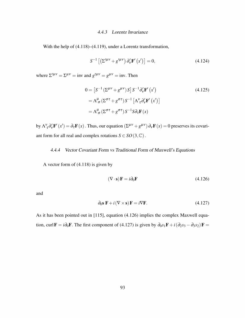
4.4.3 Lorentz Invariance
With the help of (4.118)–(4.119), under a Lorentz transformation,
S−1 [(Σ′µν +g′µν
)∂′νF′(x′)]
= 0, (4.124)
where Σ′µν = Σµν = inv and g′µν = gµν = inv. Then
0 =[S−1 (Σµν +gµν)S
]S−1
∂′νF′(x′)
(4.125)
= Λµ
σ (Σστ +gστ)S−1 [Λ
ντ∂′νF′(x′)]
= Λµ
σ (Σστ +gστ)S−1S∂τF(x)
by Λντ∂ ′νF′ (x′) = ∂τF(x) . Thus, our equation (Σµν +gµν)∂νF(x) = 0 preserves its covari-
ant form for all real and complex rotations S ∈ SO(3,C) .
4.4.4 Vector Covariant Form vs Traditional Form of Maxwell’s Equations
A vector form of (4.118) is given by
(∇ · s)F = i∂0F (4.126)
and
∂0s F+ i(∇× s)F = i∇F. (4.127)
As it has been pointed out in [115], equation (4.126) implies the complex Maxwell equa-
tion, curlF = i∂0F. The first component of (4.127) is given by ∂0s1F+ i(∂2s3−∂3s2)F =
93
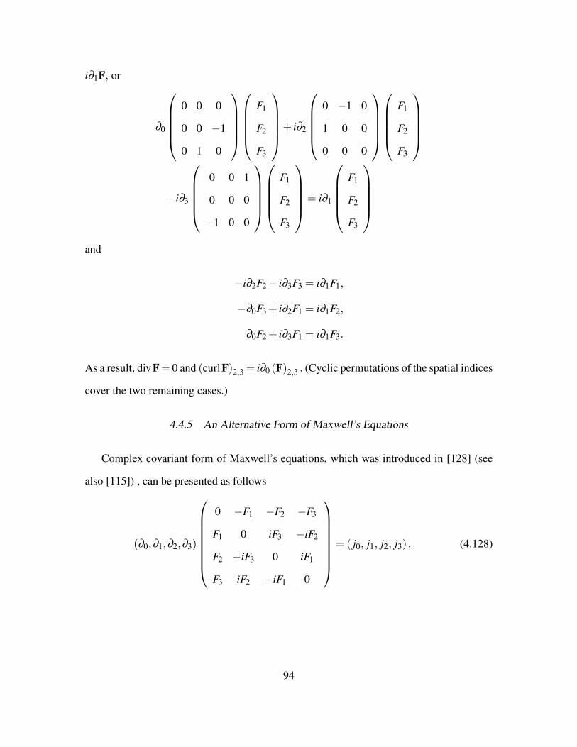
i∂1F, or
∂0
0 0 0
0 0 −1
0 1 0
F1
F2
F3
+ i∂2
0 −1 0
1 0 0
0 0 0
F1
F2
F3
− i∂3
0 0 1
0 0 0
−1 0 0
F1
F2
F3
= i∂1
F1
F2
F3
and
−i∂2F2− i∂3F3 = i∂1F1,
−∂0F3 + i∂2F1 = i∂1F2,
∂0F2 + i∂3F1 = i∂1F3.
As a result, divF= 0 and (curlF)2,3 = i∂0 (F)2,3 . (Cyclic permutations of the spatial indices
cover the two remaining cases.)
4.4.5 An Alternative Form of Maxwell’s Equations
Complex covariant form of Maxwell’s equations, which was introduced in [128] (see
also [115]) , can be presented as follows
(∂0,∂1,∂2,∂3)
0 −F1 −F2 −F3
F1 0 iF3 −iF2
F2 −iF3 0 iF1
F3 iF2 −iF1 0
= ( j0, j1, j2, j3) , (4.128)
94

or ∂Q = j, by matrix multiplication. Here, ∂ = (∂0,∂1,∂2,∂3) , j = ( j0, j1, j2, j3) , and
J = (J1,J2,J3) such that
Q = F ·J = F1
0 −1 0 0
1 0 0 0
0 0 0 i
0 0 −i 0
(4.129)
+F2
0 0 −1 0
0 0 0 −i
1 0 0 0
0 i 0 0
+F3
0 0 0 −1
0 0 i 0
0 −i 0 0
1 0 0 0
.
These matrices are transformed as a dual complex vector in C3 ,
ΛJpΛT = aqpJq, (4.130)
under a proper Lorentz transformation. In infinitesimal form,
mαβ J+J(
mαβ
)T=(
Σαβ
)TJ, (4.131)
which gives an alternative representation of the group SO(3,C) in a subspace of complex
4×4 matrices. (Details are left to the reader.)
As a result, ΛQΛT = Q′ and, in “new” coordinates, ∂ ′Q′ = j′, provided that ∂ ′ =
∂(Λ−1) and j′ = jΛT .
4.5 On Spinor Forms of Maxwell’s Equations
In conclusion, the complex matrix group SL(2,C) has a representation of the proper
orthochronous Lorentz group SO+ (1,3) by the second rank spinors.
95
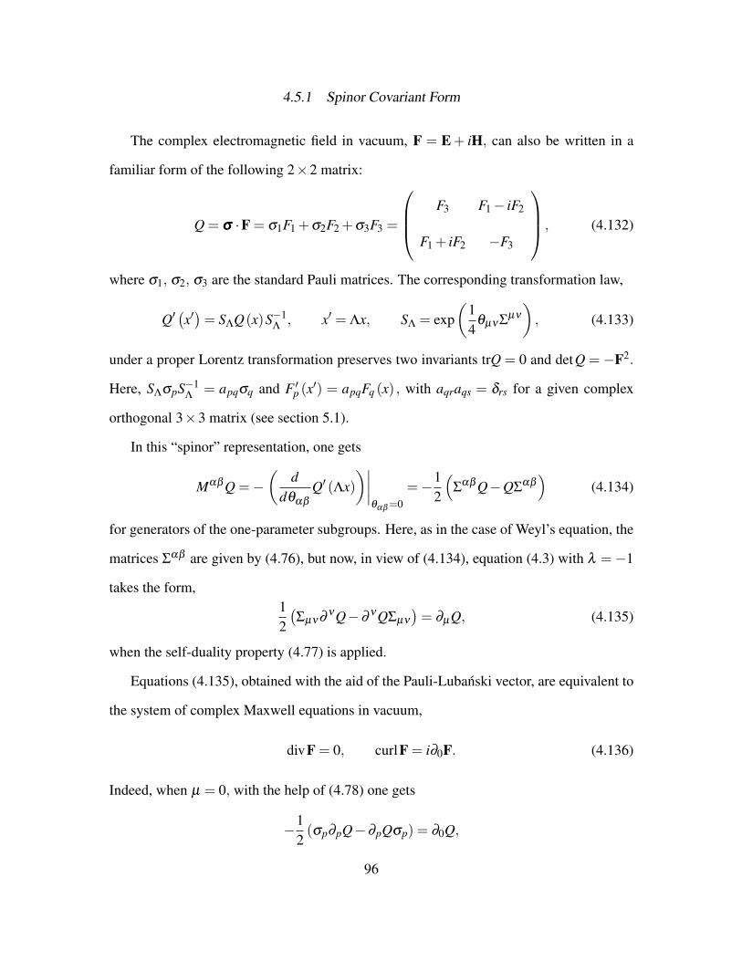
4.5.1 Spinor Covariant Form
The complex electromagnetic field in vacuum, F = E+ iH, can also be written in a
familiar form of the following 2×2 matrix:
Q = σσσ ·F = σ1F1 +σ2F2 +σ3F3 =
F3 F1− iF2
F1 + iF2 −F3
, (4.132)
where σ1, σ2, σ3 are the standard Pauli matrices. The corresponding transformation law,
Q′(x′)= SΛQ(x)S−1
Λ, x′ = Λx, SΛ = exp
(14
θµνΣµν
), (4.133)
under a proper Lorentz transformation preserves two invariants trQ = 0 and detQ = −F2.
Here, SΛσpS−1Λ
= apqσq and F ′p (x′) = apqFq (x) , with aqraqs = δrs for a given complex
orthogonal 3×3 matrix (see section 5.1).
In this “spinor” representation, one gets
Mαβ Q =−(
ddθαβ
Q′ (Λx))∣∣∣∣
θαβ=0=−1
2
(Σ
αβ Q−QΣαβ
)(4.134)
for generators of the one-parameter subgroups. Here, as in the case of Weyl’s equation, the
matrices Σαβ are given by (4.76), but now, in view of (4.134), equation (4.3) with λ =−1
takes the form,12(Σµν∂
νQ−∂νQΣµν
)= ∂µQ, (4.135)
when the self-duality property (4.77) is applied.
Equations (4.135), obtained with the aid of the Pauli-Lubanski vector, are equivalent to
the system of complex Maxwell equations in vacuum,
divF = 0, curlF = i∂0F. (4.136)
Indeed, when µ = 0, with the help of (4.78) one gets
−12(σp∂pQ−∂pQσp) = ∂0Q,
96

or
−(σpσq−σqσp
)∂pFq = 2∂0 (σrFr) ,
which gives the second complex Maxwell equation (4.136) in view of the commutation
relation,[σp,σq
]= 2iepqrσr.
When µ = p = 1,2,3, in a similar fashion,
2∂pQ = ∂0Qσp−σp∂0Q+ iepqr(∂qQσr−σr∂qQ
), (4.137)
and letting Q = Fsσs, we obtain
2∂p (Fsσs) = (σsσp−σpσs)∂0Fs
+ iepqr (σsσr−σrσs)∂qFs.
Evaluation of the commutators,
σs∂pFs = iesplσl∂0Fs + epqreslrσl∂qFs, (4.138)
and a familiar identity,
epqreslr =
∣∣∣∣∣∣∣δps δpl
δqs δql
∣∣∣∣∣∣∣= δpsδql−δplδqs, (4.139)
result in the system of Maxwell’s equations (4.136).
4.5.2 Traditional Spinor Form of Maxwell’s Equations
Equations (4.135), that are obtained here with the help of the Pauli-Lubanski vector,
give an alternative (vacuum) version of the spinor form of Maxwell’s equations,
(∂0 +σσσ ·∇)(σσσ ·F) = j0 +σσσ · j, (4.140)
97
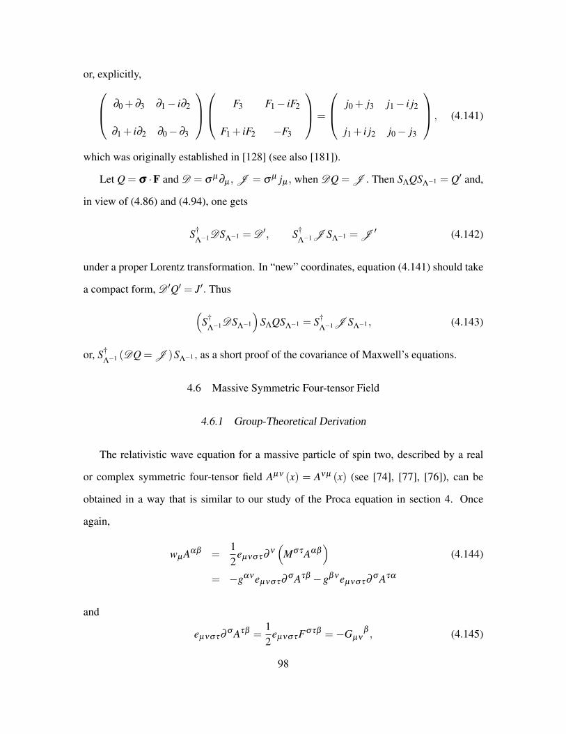
or, explicitly, ∂0 +∂3 ∂1− i∂2
∂1 + i∂2 ∂0−∂3
F3 F1− iF2
F1 + iF2 −F3
=
j0 + j3 j1− i j2
j1 + i j2 j0− j3
, (4.141)
which was originally established in [128] (see also [181]).
Let Q = σσσ ·F and D = σ µ∂µ , J = σ µ jµ , when DQ = J . Then SΛQSΛ−1 = Q′ and,
in view of (4.86) and (4.94), one gets
S†Λ−1DSΛ−1 = D ′, S†
Λ−1J SΛ−1 = J ′ (4.142)
under a proper Lorentz transformation. In “new” coordinates, equation (4.141) should take
a compact form, D ′Q′ = J′. Thus(S†
Λ−1DSΛ−1
)SΛQSΛ−1 = S†
Λ−1J SΛ−1, (4.143)
or, S†Λ−1 (DQ = J )SΛ−1, as a short proof of the covariance of Maxwell’s equations.
4.6 Massive Symmetric Four-tensor Field
4.6.1 Group-Theoretical Derivation
The relativistic wave equation for a massive particle of spin two, described by a real
or complex symmetric four-tensor field Aµν (x) = Aνµ (x) (see [74], [77], [76]), can be
obtained in a way that is similar to our study of the Proca equation in section 4. Once
again,
wµAαβ =12
eµνστ∂ν
(MστAαβ
)(4.144)
= −gανeµνστ∂σ Aτβ −gβνeµνστ∂
σ Aτα
and
eµνστ∂σ Aτβ =
12
eµνστFστβ =−G β
µν , (4.145)
98
where, by definition, Fστβ = ∂ σ Aτβ −∂ τAσβ and eµνστFστβ =−2G β
µν . Thus
wµAαβ = gανG β
µν +gβνG αµν , (4.146)
or
wµAαβ = Gµαβ +Gµβα , wµAαβ = Gµαβ +Gµβα (4.147)
and
w2Aαβ = wµ
(wµAαβ
)= wµGµαβ +wµGµβα . (4.148)
In a similar fashion, one can show that
wµGµαβ = 2∂νFναβ +∂νFνβα (4.149)
+∂α
(Fβστgστ
)−gαβ
∂ν (Fνστgστ) ,
as a result of an elementary but rather tedious four-tensor algebra calculation with the help
of a familiar relation
eµνστeµκλρ =−
∣∣∣∣∣∣∣∣∣∣δ ν
κ δ ν
λδ ν
ρ
δ σκ δ σ
λδ σ
ρ
δ τκ δ τ
λδ τ
ρ
∣∣∣∣∣∣∣∣∣∣. (4.150)
For a massive spin-2 field, the second Casimir operator is equal to w2Aαβ =−6m2Aαβ ,
and we obtain
∂νFναβ +∂νFνβα − 23
gαβ∂ν (Fνστgστ) (4.151)
+13
∂α
(Fβστgστ
)+
13
∂β (Fαστgστ) =−2m2Aαβ ,
where
Fναβ = ∂νAαβ −∂
αAνβ =−Fανβ , (4.152)
Fνστgστ = ∂νA−∂τAντ , A = gστAστ ,
and Fαβγ +Fβγα +Fγαβ = 0 provided Aαβ = Aβα .
99
In terms of potentials, one gets
∂2Aαβ − 2
3
(∂
α∂νAνβ +∂
β∂νAνα
)+
13
∂α
∂β A (4.153)
−13
gαβ(∂
2A−∂µ∂νAµν)=−m2Aαβ ,
with ∂µ∂νAµν = 0, if m > 0, in view of
0≡ w2 (∂µ∂νAµν
)= ∂µ∂ν
(w2Aµν
)=−6m2
∂µ∂νAµν .
The same results can be derived by differentiation from (4.151) or, independently, with the
help of an operator identity
w2 =−12
∂2 (MστMστ)−∂µ∂
ν (Mµσ Mσν) .
Moreover, equation (4.153) is reduced to
2(
∂α
∂νAνβ +∂β
∂νAνα
)−∂
α∂
β A+gαβ∂
2A = 0 (4.154)
with the help of the first Casimir operator, ∂ 2Aαβ =−m2Aαβ . Multiplication of (4.154) by
gαβ with contraction over two repeated indices results in ∂ 2A = 0. Then A = 0, due to
0 = ∂2A = ∂
2 (gµνAµν)= gµν∂
2 (Aµν) =−m2A, m > 0.
Thus, the system of wave equations for a massive spin-2 particle has the form
∂2Aµν +m2Aµν = 0, ∂
α
(∂νAνβ
)+∂
β (∂νAνα) = 0, (4.155)
subject to A = gµνAµν = ∂µ∂νAµν = 0. It is worth noting, once again, that we have derived
these equations by using the Pauli-Lubanski vector and the relativistic definition of mass
and spin in terms of Casimir operators of the Poincare group.
In the massless limit m→ 0, instead of (4.155), one has ∂ 2Aµν = 0 and ∂ 2A = 0 subject
to
∂α
(∂νAνβ − 1
4∂
β A)+∂
β
(∂νAνα − 1
4∂
αA)=
12
gαβ∂µ∂νAµν , (4.156)
100
in a similar fashion. Moreover, if m= 0, equation (4.151) is invariant under a familiar gauge
transformation Aαβ → A′αβ
+∂α fβ +∂β fα provided that ∂ ν (∂ν fα −∂α fν) = 0 (Maxwell’s
equations in vacuum).
4.6.2 An Alternative Gauge Condition
In view of the following identity,
∂α
(∂νAνβ − 1
4∂
β A)+∂
β
(∂νAνα − 1
4∂
αA)
= ∂α
∂νAνβ +∂β
∂νAνα − 12
∂α
∂β A,
one can impose another condition,
4∂νAµν −∂µA = 0, (4.157)
in order to simplify (4.153):
∂2Aµν − 1
4gµν
∂2A =−m2Aµν . (4.158)
Moreover, by contraction,9
0≡ ∂2A− 1
4gµνgµν
∂2A =−m2A, A = gστAστ = 0,
if m > 0. As a result, we obtain
∂2Aµν +m2Aµν = 0, ∂νAµν = ∂νAνµ = 0. (4.159)
These equations were originally introduced by Fierz and Pauli [74], [77], [76] with the help
of a Lagrangian approach. It is worth noting that our equations (4.155) are necessary and
sufficient with the relativistic definition of mass and spin-2 of the field in question, whereas
traditional equations (4.159) give only sufficient conditions.
9Condition A = 0 is not required in the massless limit.
101
In addition, it should be noted that from (4.155) subject to A= gµνAµν = ∂µ∂νAµν = 0,
it follows that
∂2 (∂νAνµ)+m2 (∂νAνµ) = 0, ∂
α
(∂ν∂β Aνβ
)+∂
2 (∂νAνα) = 0.
Combining the latter equations, in turn, gives ∂νAνµ = 0 for m > 0. On the other hand,
if the original Fierz-Pauli equations (4.159) are satisfied, then the equations (4.155) also
hold.
4.6.3 Fierz-Pauli vs Maxwell’s Equations
When m = 0, one gets
∂νFµνα = ∂ν (∂µAνα −∂
νAµα) = ∂µ (∂νAνα)−∂
2Aµα = 0, (4.160)
subject to (4.159). In addition,
∂λ Fστα +∂σ Fτλα +∂τFλσα = 0, (4.161)
which follows from definition. These facts allow one to represent the massless Fierz-Pauli
equations in terms of the third rank field tensor, somewhat similar to classical electrody-
namics. Indeed, by analogy with Maxwell’s equations, we obtain
∂νFµνα = 0, ∂νGµνα = 0 (4.162)
in view of 2Gµνα =−eµνστF αστ and
∂νGµνα =−16
eµνστ (∂νF αστ +∂σ F α
τν +∂τF ανσ ) = 0
(for every fixed α = 0,1,2,3).
Finally, both pairs of these equations can be combined together in the following com-
plex form
∂νQµνα = 0, Qµνα = Fµνα − i2
eµνστF αστ , (4.163)
102
with the help of a self-dual complex four-tensor:
2iQµνα = eµνστQ αστ , eµνστQστα = 2iQ α
µν . (4.164)
The covariant field “energy-momentum” tensor and the corresponding differential balance
equation,∂
∂xν
(Q∗
µλσQλνσ +Qµλσ
∗Qλνσ
)= 0, (4.165)
can be derived in a complete analogy with complex electrodynamics [115], [116].
4.6.4 Fierz-Pauli vs Linearized Einstein’s Equations
In general relativity, the linearized equations for a weak gravitational field [61], [96],
namely,
∂µ∂σ hσν +∂ν∂
σ hσ µ −∂µ∂νh (4.166)
−∂2hµν −gµν
(∂σ ∂τhστ −∂
2h)= 0,
describe small deviations from the flat Minkowski metric, gµν = diag(1,−1,−1,−1) , on
the pseudo-Riemannian manifold subject to a gauge condition
2∂νhµν −∂µh = 0, h = gστhστ (4.167)
(see, for example, [46], [69], [76], [82], [97], [108], [122], [157], [167], [219], [220], [225],
[227], [229], [232], [237], and the references therein for more details).
Our calculations have shown that linearized Einstein’s equations (4.166) do not coin-
cide with the massless limit of the spin-2 particle wave equation (4.153). But they can be
reduced to the massless case of the Fierz-Pauli equations (4.159) in view of an additional
condition (4.167) on a certain solution set. In the literature, this fact is usually interpreted as
spin-2 for a graviton although, from the group-theoretical point of view, this massless limit
yet requires certain analysis of helicity, say similar to the one in electrodynamics [115],
which will be discuss elsewhere.
103
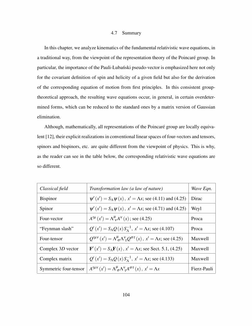
4.7 Summary
In this chapter, we analyze kinematics of the fundamental relativistic wave equations, in
a traditional way, from the viewpoint of the representation theory of the Poincare group. In
particular, the importance of the Pauli-Lubanski pseudo-vector is emphasized here not only
for the covariant definition of spin and helicity of a given field but also for the derivation
of the corresponding equation of motion from first principles. In this consistent group-
theoretical approach, the resulting wave equations occur, in general, in certain overdeter-
mined forms, which can be reduced to the standard ones by a matrix version of Gaussian
elimination.
Although, mathematically, all representations of the Poincare group are locally equiva-
lent [12], their explicit realizations in conventional linear spaces of four-vectors and tensors,
spinors and bispinors, etc. are quite different from the viewpoint of physics. This is why,
as the reader can see in the table below, the corresponding relativistic wave equations are
so different.
Classical field Transformation law (a law of nature) Wave Eqn.
Bispinor ψ ′ (x′) = SΛψ (x) , x′ = Λx; see (4.11) and (4.25) Dirac
Spinor ψ ′ (x′) = SΛψ (x) , x′ = Λx; see (4.71) and (4.25) Weyl
Four-vector A′µ (x′) = Λµ
νAν (x) ; see (4.25) Proca
“Feynman slash” Q′ (x′) = SΛQ(x)S−1Λ
, x′ = Λx; see (4.107) Proca
Four-tensor Q′µν (x′) = Λµ
σ ΛντQστ (x) , x′ = Λx; see (4.25) Maxwell
Complex 3D vector F′ (x′) = SΛF(x) , x′ = Λx; see Sect. 5.1, (4.25) Maxwell
Complex matrix Q′ (x′) = SΛQ(x)S−1Λ
, x′ = Λx; see (4.133) Maxwell
Symmetric four-tensor A′µν (x′) = Λµ
σ ΛντAστ (x) , x′ = Λx Fierz-Pauli
104
Chapter 5
WAVE FUNCTIONS FOR GENERALIZED HARMONIC OSCILLATORS
In this chapter, the time-dependent Schrodinger equation for the most general variable
quadratic Hamiltonians is transformed into a standard autonomous form. As a result, the
time evolution of exact wave functions of generalized harmonic oscillators is determined
in terms of the solutions of certain Ermakov and Riccati-type systems. The Ermakov-type
system is introduced here (see also [125]) and has become a major mathematical tool for
paraxial optics and radiation field quantization in variable media with applications to quan-
tum optics and possibly to the study of gravitational wave detection. In addition, it is shown
that the classical Arnold transform is naturally connected with Ehrenfest’s theorem for gen-
eralized harmonic oscillators. Quantum systems with variable quadratic Hamiltonians are
called the generalized harmonic oscillators (see [20], [41], [53], [54], [68], [73], [92],
[129], [132], [148], [151], [233], [235], [238] and references therein). These systems have
attracted substantial attention over the years because of their great importance in many ad-
vanced quantum problems. Examples are coherent states and uncertainty relations, Berry’s
phase, quantization of mechanical systems and Hamiltonian cosmology. More applica-
tions include, but are not limited to charged particle traps and motion in uniform magnetic
fields, molecular spectroscopy and polyatomic molecules in varying external fields, crys-
tals through which an electron is passing and exciting the oscillator modes, and other mode
interactions with external fields. Quadratic Hamiltonians have particular applications in
quantum electrodynamics because the electromagnetic field can be represented as a set of
forced harmonic oscillators [73].
A goal of this chapter is to construct exact wave functions for generalized (driven) har-
monic oscillators [20], [39], [92], [129], [132], [233], [235], in terms of Hermite polyno-
105

mials by transforming the time-dependent Schrodinger equation into an autonomous form
[238]. The relationship with certain Ermakov and Riccati-type systems, which seems to be
missing in the available literature in general, is investigated. A group theoretical approach
to a similar class of partial differential equations is discussed in Refs. [2], [38], [44], [83],
[153], [179] (see also [200], [201] and references therein). Some applications to the nonlin-
ear Schrodinger equation can also be found in Refs. [45], [103], [104], [109], [120], [172],
[199] and [203].
5.1 Transforming Generalized Harmonic Oscillators into Autonomous Form
We consider the one-dimensional time-dependent Schrodinger equation
i∂ψ
∂ t= Hψ, in (5.1)
where the variable Hamiltonian H = Q(p,x) is an arbitrary quadratic of two operators
p =−i∂/∂x and x, namely,
iψt =−a(t)ψxx +b(t)x2ψ− ic(t)xψx− id (t)ψ− f (t)xψ + ig(t)ψx, (5.2)
(a, b, c, d, f and g are suitable real-valued functions of time only). We shall refer to
these quantum systems as the generalized (driven) harmonic oscillators. Some examples,
a general approach and known elementary solutions can be found in Refs. [39], [40], [41],
[43], [53], [70], [72], [73], [132], [135], [150], [198], [233] and [235]. In addition, a case
related to Airy functions is discussed in [126] and Ref. [42] deals with another special case
of transcendental solutions.
The following is our first result.
Lemma 5.1.1 The substitution
ψ =ei(α(t)x2+δ (t)x+κ(t))√
µ (t)χ (ξ ,τ) , ξ = β (t)x+ ε (t) , τ = γ (t) (5.3)
106

transforms the non-autonomous and inhomogeneous Schrodinger equation (5.2) into the
autonomous form
−iχτ =−χξ ξ + c0ξ2χ (c0 = 0,1) (5.4)
provided thatdα
dt+b+2cα +4aα
2 = c0aβ4, (5.5)
dβ
dt+(c+4aα)β = 0, (5.6)
dγ
dt+aβ
2 = 0 (5.7)
anddδ
dt+(c+4aα)δ = f +2gα +2c0aβ
3ε, (5.8)
dε
dt= (g−2aδ )β , (5.9)
dκ
dt= gδ −aδ
2 + c0aβ2ε
2. (5.10)
Here
α =1
4aµ ′
µ− d
2a. (5.11)
Proof Differentiating ψ = µ−1/2 (t)eiS(x,t)χ (ξ ,τ) with S = α (t)x2 + δ (t)x+κ (t) , ξ =
β (t)x+ ε (t) and τ = γ (t) yields
ie−iSψt =
1√
µ
[−(α′x2 +δ
′x+κ′)
χ + i((
β′x+ ε
′)χξ + γ
′χτ −
µ ′
2µχ
)], (5.12)
e−iSψx =
1√
µ
[i(2αx+δ )χ +β χξ
](5.13)
and
e−iSψxx =
1√
µ
[(2iα− (2αx+δ )2
)χ +2i(2αx+δ )β χξ +β
2χξ ξ
]. (5.14)
Substituting into
iψt = −aψxx +(b− c0aβ
4)x2ψ− icxψx− idψ (5.15)
−(
f +2c0aβ3ε)
xψ + igψx− c0aβ2ε
2ψ + c0aβ
2ε
2ξ
2ψ
107
and using system (5.5)–(5.10), results in Eq. (5.4). A computer algebra proof is given in
[112].
Our transformation (5.3) provides a new interpretation to system (5.5)–(5.10) originally
derived in Ref. [39] when c0 = 0 by integrating the corresponding Schrodinger equation
via the Green function method (see also [202] for an eigenfunction expansion). Here, we
discuss the case c0 6= 0 as its natural extension.
The substitution (5.11), which has been already used in [39], appears here from a new
“transformation perspective”. It now reduces the inhomogeneous equation (5.5) to the
second order ordinary differential equation
µ′′− τ (t)µ
′+4σ (t)µ = c0 (2a)2β
4µ, (5.16)
that has the familiar time-varying coefficients
τ (t) =a′
a−2c+4d, σ (t) = ab− cd +d2 +
d2
(a′
a− d′
d
). (5.17)
(The reader should be convinced that this derivation is rather straightforward.)
When c0 = 0, equation (5.5) is called the Riccati nonlinear differential equation [222],
[230]; consequently, the system (5.5)–(5.10) shall be referred to as a Riccati-type system.
(Similar terminology is used in [201] for the corresponding parabolic equation.) Now if
c0 = 1, equation (5.16) can be reduced to a generalized version of the Ermakov nonlinear
differential equation (5.50) (see, for example, [41], [66], [130], [202] and references therein
regarding Ermakov’s equation) and we shall refer to the corresponding system (5.5)–(5.10)
with c0 6= 0 as an Ermakov-type system.
5.2 Green’s Function and Wavefunctions
Two particular solutions of the time-dependent Schrodinger equation (5.2) are useful
in physical applications. Using standard oscillator wave functions for equation (5.4) when
108

c0 = 1 (for example, [79], [123] and/or [152]) results in the solution
ψn (x, t) =ei(αx2+δx+κ)+i(2n+1)γ√
2nn!µ√
πe−(βx+ε)2/2 Hn (βx+ ε) , (5.18)
where Hn (x) are the Hermite polynomials [162], provided that the solution of the Ermakov-
type system (5.5)–(5.10) is available.
The Green function of generalized harmonic oscillators has been constructed in the
following fashion in Ref. [39]:
G(x,y, t) =1√
2πiµ0 (t)exp[i(α0 (t)x2 +β0 (t)xy+ γ0 (t)y2 +δ0 (t)x+ ε0 (t)y+κ0 (t)
)].
(5.19)
The time-dependent coefficients α0, β0, γ0, δ0, ε0, κ0 satisfy the Riccati-type system (5.5)–
(5.10) (c0 = 0) and are given as follows [39], [198], [202]:
α0 (t) =1
4a(t)µ ′0 (t)µ0 (t)
− d (t)2a(t)
, (5.20)
β0 (t) =−λ (t)µ0 (t)
, λ (t) = exp(−∫ t
0(c(s)−2d (s)) ds
), (5.21)
γ0 (t) =1
2µ1 (0)µ1 (t)µ0 (t)
+d (0)2a(0)
(5.22)
and
δ0 (t) =λ (t)µ0 (t)
∫ t
0
[(f (s)− d (s)
a(s)g(s)
)µ0 (s)+
g(s)2a(s)
µ′0 (s)
]ds
λ (s), (5.23)
ε0 (t) = −2a(t)λ (t)µ ′0 (t)
δ0 (t)+8∫ t
0
a(s)σ (s)λ (s)(µ ′0 (s)
)2 (µ0 (s)δ0 (s)) ds (5.24)
+2∫ t
0
a(s)λ (s)µ ′0 (s)
(f (s)− d (s)
a(s)g(s)
)ds,
κ0 (t) =a(t)µ0 (t)
µ ′0 (t)δ
20 (t)−4
∫ t
0
a(s)σ (s)(µ ′0 (s)
)2 (µ0 (s)δ0 (s))2 ds (5.25)
−2∫ t
0
a(s)µ ′0 (s)
(µ0 (s)δ0 (s))(
f (s)− d (s)a(s)
g(s))
ds
109
(δ0 (0) = −ε0 (0) = g(0)/(2a(0)) and κ0 (0) = 0) provided that µ0 and µ1 are standard
solutions of equation (5.16) with c0 = 0 corresponding to the initial conditions µ0 (0) =
0, µ ′0 (0) = 2a(0) 6= 0 and µ1 (0) 6= 0, µ ′1 (0) = 0. (Proofs of these facts are outlined in
Refs. [39], [42] and [198]. See also important previous works [54], [148], [233], [235],
[238] and references therein for more details.)
Hence, the corresponding Cauchy initial value problem can be solved (formally) by the
superposition principle:
ψ (x, t) =∫
∞
−∞
G(x,y, t)ψ (y,0) dy (5.26)
for some suitable initial data ψ (x,0) = ϕ (x) (see Refs. [39], [198] and [202] for further
details).
In particular, using the wave functions (5.18) we get the integral
ψn (x, t) =∫
∞
−∞
G(x,y, t)ψn (y,0) dy, (5.27)
and this can be evaluated by
∫∞
−∞
e−λ 2(x−y)2Hn (ay) dy (5.28)
=
√π
λ n+1
(λ
2−a2)n/2Hn
(λax
(λ 2−a2)1/2
), Reλ
2 > 0,
which is an integral transform equivalent to Eq. (30) on page 195 of Vol. 2 of Ref. [64] (the
Gauss transform of Hermite polynomials), or Eq. (17) on page 290 of Vol. 2 of Ref. [65].
5.3 Solution to Ermakov-type System
As shown in the previous section, the time evolution of the wave functions (5.18) is de-
termined in terms of the solution to the initial value problem for the Ermakov-type system.
In this section, formulas (5.18)–(5.19) and (5.27)–(5.28) shall be used in order to solve the
general system (5.5)–(5.10) when c0 6= 0 along with the uniqueness property of the Cauchy
110
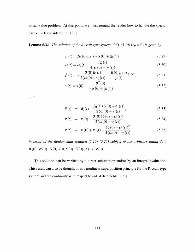
initial value problem. At this point, we must remind the reader how to handle the special
case c0 = 0 considered in [198].
Lemma 5.3.1 The solution of the Riccati-type system (5.5)–(5.10) (c0 = 0) is given by
µ (t) = 2µ (0)µ0 (t)(α (0)+ γ0 (t)) , (5.29)
α (t) = α0 (t)−β 2
0 (t)4(α (0)+ γ0 (t))
, (5.30)
β (t) =− β (0)β0 (t)2(α (0)+ γ0 (t))
=β (0)µ (0)
µ (t)λ (t) , (5.31)
γ (t) = γ (0)− β 2 (0)4(α (0)+ γ0 (t))
(5.32)
and
δ (t) = δ0 (t)−β0 (t)(δ (0)+ ε0 (t))
2(α (0)+ γ0 (t)), (5.33)
ε (t) = ε (0)− β (0)(δ (0)+ ε0 (t))2(α (0)+ γ0 (t))
, (5.34)
κ (t) = κ (0)+κ0 (t)−(δ (0)+ ε0 (t))
2
4(α (0)+ γ0 (t))(5.35)
in terms of the fundamental solution (5.20)–(5.25) subject to the arbitrary initial data
µ (0) , α (0) , β (0) 6= 0, γ (0) , δ (0) , ε (0) , κ (0).
This solution can be verified by a direct substitution and/or by an integral evaluation.
This result can also be thought of as a nonlinear superposition principle for the Riccati-type
system and the continuity with respect to initial data holds [198].
111

Hence, the solution (5.29)–(5.35) implies the following asymptotics established in [198]:
α0 (t) =1
4a(0) t− c(0)
4a(0)− a′ (0)
8a2 (0)+O (t) , (5.36)
β0 (t) =−1
2a(0) t+
a′ (0)4a2 (0)
+O (t) , (5.37)
γ0 (t) =1
4a(0) t+
c(0)4a(0)
− a′ (0)8a2 (0)
+O (t) , (5.38)
δ0 (t) =g(0)
2a(0)+O (t) , ε0 (t) =−
g(0)2a(0)
+O (t) , (5.39)
κ0 (t) = O (t) (5.40)
as t → 0 for sufficiently smooth coefficients of the original Schrodinger equation (5.2).
Therefore,
G(x,y, t) ∼ 1√2πia(0) t
exp
[i(x− y)2
4a(0) t
](5.41)
×exp[−i(
a′ (0)8a2 (0)
(x− y)2 +c(0)
4a(0)(x2− y2)− g(0)
2a(0)(x− y)
)]as t→ 0 (where f ∼ g as t→ 0, if limt→0 ( f/g) = 1). This corrects an errata in Ref. [39] .
Finally, we present the extension to a general case when c0 6= 0. Our main result is the
following. Computer algebra proofs of these results can be found in [112].
Lemma 5.3.2 The solution of the Ermakov-type system (5.5)–(5.10) when c0 = 1(6= 0) is
given by
µ = µ (0)µ0
√β 4 (0)+4(α (0)+ γ0)
2, (5.42)
α = α0−β20
α (0)+ γ0
β 4 (0)+4(α (0)+ γ0)2 , (5.43)
β =− β (0)β0√β 4 (0)+4(α (0)+ γ0)
2=
β (0)µ (0)µ (t)
λ (t) , (5.44)
γ = γ (0)− 12
arctanβ 2 (0)
2(α (0)+ γ0), a(0)> 0 (5.45)
112

and
δ = δ0−β0ε (0)β 3 (0)+2(α (0)+ γ0)(δ (0)+ ε0)
β 4 (0)+4(α (0)+ γ0)2 , (5.46)
ε =2ε (0)(α (0)+ γ0)−β (0)(δ (0)+ ε0)√
β 4 (0)+4(α (0)+ γ0)2
, (5.47)
κ = κ (0)+κ0− ε (0)β3 (0)
δ (0)+ ε0
β 4 (0)+4(α (0)+ γ0)2 (5.48)
+(α (0)+ γ0)ε2 (0)β 2 (0)− (δ (0)+ ε0)
2
β 4 (0)+4(α (0)+ γ0)2
in terms of the fundamental solution (5.20)–(5.25) subject to the arbitrary initial data
µ (0) , α (0) , β (0) 6= 0, γ (0) , δ (0) , ε (0) , κ (0) .
Following are the steps to the sketch of the proof. Evaluate the integral (5.27) with the
help of (5.28) by completing the square and simplify. Use the uniqueness property of the
Cauchy initial value problem. One can also verify our solution by a direct substitution into
the system (5.5)–(5.10) when c0 = 1. These elementary but rather tedious calculations are
left to the reader (the use of a computer algebra system is helpful at certain steps).
Furthermore, the asymptotics (5.36)–(5.40) together with our formulas (5.42)–(5.48)
result in the continuity with respect to initial data:
limt→0+
µ (t) = µ (0) , limt→0+
α (t) = α (0) , etc. (5.49)
Thus the transformation property (5.42)–(5.48) allows us to find a solution of the initial
value problem in terms of the fundamental solution (5.20)–(5.25) and it may be referred to
as a nonlinear superposition principle for the Ermakov-type system.
5.4 Solution of the Ermakov-type Equation
Starting from (5.16)–(5.17) when c0 = 1, and using (5.44) we arrive at
µ′′− τ (t)µ
′+4σ (t)µ = (2a)2 (β (0)µ (0)λ )4µ−3, (5.50)
113
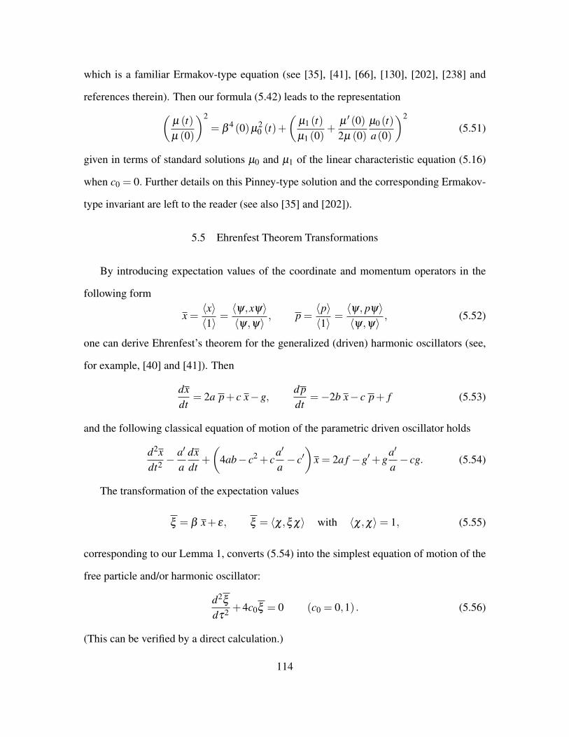
which is a familiar Ermakov-type equation (see [35], [41], [66], [130], [202], [238] and
references therein). Then our formula (5.42) leads to the representation(µ (t)µ (0)
)2
= β4 (0)µ
20 (t)+
(µ1 (t)µ1 (0)
+µ ′ (0)2µ (0)
µ0 (t)a(0)
)2
(5.51)
given in terms of standard solutions µ0 and µ1 of the linear characteristic equation (5.16)
when c0 = 0. Further details on this Pinney-type solution and the corresponding Ermakov-
type invariant are left to the reader (see also [35] and [202]).
5.5 Ehrenfest Theorem Transformations
By introducing expectation values of the coordinate and momentum operators in the
following form
x =〈x〉〈1〉
=〈ψ,xψ〉〈ψ,ψ〉
, p =〈p〉〈1〉
=〈ψ, pψ〉〈ψ,ψ〉
, (5.52)
one can derive Ehrenfest’s theorem for the generalized (driven) harmonic oscillators (see,
for example, [40] and [41]). Then
dxdt
= 2a p+ c x−g,d pdt
=−2b x− c p+ f (5.53)
and the following classical equation of motion of the parametric driven oscillator holds
d2xdt2 −
a′
adxdt
+
(4ab− c2 + c
a′
a− c′
)x = 2a f −g′+g
a′
a− cg. (5.54)
The transformation of the expectation values
ξ = β x+ ε, ξ = 〈χ,ξ χ〉 with 〈χ,χ〉= 1, (5.55)
corresponding to our Lemma 1, converts (5.54) into the simplest equation of motion of the
free particle and/or harmonic oscillator:
d2ξ
dτ2 +4c0ξ = 0 (c0 = 0,1) . (5.56)
(This can be verified by a direct calculation.)
114
Remark An exact transformation of a linear second-order differential equation into the
equation of motion of free particle was discussed by Arnold [9]. An extension of the later
to the case of the time-dependent Schrodinger equation had been considered, for exam-
ple, in Ref. [238] and recently it has been reproduced as the quantum Arnold transforma-
tion in [7] and [91] (see also [2], [38], [44], [83], [120], [153], [179], [201] and [203]
for similar transformations of nonlinear Schrodinger and other equations of mathematical
physics). We elaborate on a relation of the quantum Arnold transformation for the general-
ized (driven) harmonic oscillators with a Riccati-type system when c0 = 0 (transformation
to the free particle) and consider an extension of this transformation (in terms of solutions
of the corresponding Ermakov-type system) to the case c0 = 1 (transformation to the clas-
sical harmonic oscillator [238]).
5.6 Conclusion
In this chapter, we have determined the time evolution of the wave functions of gen-
eralized (driven) harmonic oscillators (5.18), known for their great importance in many
advanced quantum problems [73], in terms of the solution to the Ermakov-type system
(5.5)–(5.10) by means of a variant of the nonlinear superposition principle (5.42)–(5.48).
In this approach, the standard solutions of equation (5.16) with c0 = 0 should be found
analytically or numerically. Moreover, the classical Arnold transformation is related to
Ehrenfest’s theorem. Numerous examples, the corresponding coherent states, dynamic in-
variants, eigenfunction expansions and transition amplitudes [53], [54], [126], [129], [132],
[148], [147], [202] will be discussed elsewhere.
115
Chapter 6
A MODEL FOR RADIATION FIELD QUANTIZATION IN MEDIA
The quantization of an electromagnetic field in an inhomogeneous and time variable
medium is discussed via the Caldirola-Kanai Hamiltonian. This model was also discussed
from a different perspective in [41]. Here, we describe a multi-parameter family of squeezed
states for this standard model of damping in non-relativistic quantum mechanics and dis-
cuss the uncertainty relation. The time-dependent photon statistics for the Caldirola-Kanai
Hamiltonian are given explicitly in the Schrodinger picture in terms of the solution of the
Ermakov-type system, see Chapter 5 or [125]. The Caldirola-Kanai Hamiltonian arises
naturally through the quantization of the electromagnetic field from Maxwell’s equations
in a medium with certain properties that will be specified below.
For the quantization of a classical Hamiltonian system one replaces canonically con-
jugate coordinates and momenta by time-dependent operators qλ (t) and pλ (t) that satisfy
the commutation relations
[qλ (t),qµ(t)] = [pλ (t), pµ(t)] = 0, [qλ (t), pµ(t)] = ihδλ µ . (6.1)
The time-evolution of these operators is determined by the Heisenberg equation of motion
ddt
qλ (t) =ih[qλ (t),H ],
ddt
pλ (t) =ih[pλ (t),H ], (6.2)
For the phenomenological Maxwell equations in linear, dispersive, time-varying media,
namely
curlE =−1c
∂B∂ t
, divD = 4πρ, (6.3)
curlH =1c
∂D∂ t
+4π
cj, divB = 0, (6.4)
116
D = ε(r, t)E, B = µ(r, t)H, j = σ(r, t)E, (6.5)
the continuity equation,
∂ρ
∂ t+div j =
∂ρ
∂ t+
4πσ
ερ +D ·grad
(σ
ε
)= 0, (6.6)
has the stationary solution ρ ≡ 0 under the condition grad(σ/ε) = 0.
With the help of the vector A and scalar ϕ potentials,
B = curlA, E =−1c
∂A∂ t
+gradϕ, (6.7)
the Maxwell equations can be reduced to the gauge condition
1c
div(
ε∂A∂ t
)= div(ε gradϕ) (6.8)
and the single second-order generalized wave equation
curl(µ−1 curlA
)+
1c2
∂
∂ t
(ε
∂A∂ t
)+
4πσ
c2∂A∂ t
=1c
∂
∂ t(ε gradϕ)+
4πσ
cgradϕ. (6.9)
Here, we consider the factorized (real-valued) dielectric permittivity, the magnetic perme-
ability, and the conductivity (tensors)
ε(r, t) = ξ (t)ε(r), µ(r, t) = η(t)µ(r), σ(r, t) = χ(t)σ(r) (6.10)
(the case σ ≡ 0 was discussed in [56]). Under the imposed condition grad(σ/ε) = 0, one
can choose 4πσ = ε without loss of generality.
The solution of the classical problem for a given single mode, υ say, has the form
A(r, t) = u(r)q(t), ϕ(r, t) = (k/c)dqdt
φ(r)
(k is a constant), and
B = qcurlU, D =−ξ
cdqdt
εU, (6.11)
117

provided that
curl(
1µ
curlU)= υ
2εU, U = u− k gradφ ,
d2qdt2 +
ξ ′+χ
ξ
dqdt
+c2υ2
ξ ηq = 0, υ = constant, (6.12)
and certain required boundary conditions are satisfied on the boundary of the cavity (see
[56], [57], for more details).
Thus we can choose c = d = f = g = 0 and
a =1
2ξe−
∫(χ/ξ )dt , b =
c2υ2
2ηe∫(χ/ξ )dt (6.13)
in the Hamiltonian
H = a(t)p2 +b(t)x2 + c(t)x p− id(t)− f (t)x−g(t)p. (6.14)
For a general approach see [4], [118], [114].
6.1 Exact Wave Functions and the Ermakov-type System
Motivated by (6.3)-(6.14), we consider the time-dependent Schrodinger equation in one
dimension with the Caldirola-Kanai Hamiltonian,
iψt =ω0
2
(−e−2λ t
ψxx + x2 e2λ tψ
)+ iεxψx, (6.15)
which has the following square integrable solution (wave function)
ψn (x, t) =ei(α(t)x2+δ (t)x+κ(t)+γ(t))√
2nn!µ (t)√
πe−(β (t)x+ε(t))2/2Hn (β (t)x+ ε(t)) , (6.16)
where α,β ,γ,δ ,κ,and ε are determined by the Ermakov-type system (5.5)–(5.10) and are
given explicitly on the next page:
118

µ (t) = µ (0)e−(λ−ε)t√
β 40 ω2
0 sin2(ωt)+((2α0ω0 +λ − ε)sin(ωt)+ω cos(ωt))2
α (t) = e2λ t ν cos(2ωt)+ωω0(4α2
0 +β 40 −1
)sin(2ωt)/4+α0ω2−ν
β 40 ω2
0 sin2(ωt)+((2α0ω0 +λ − ε)sin(ωt)+ω cos(ωt))2
β (t) =β0ωeλ t√
β 40 ω2
0 sin2(ωt)+((2α0ω0 +λ − ε)sin(ωt)+ω cos(ωt))2,
γ (t) = γ0−12
arctanω0β 2
0 tan(ωt)ω +(2α0ω0 +λ − ε) tan(ωt)
,
δ (t) = ωeλ t ω0ε0β 30 sin(ωt)+δ0 ((2α0ω0 +λ − ε)sin(ωt)+ω cos(ωt))
β 40 ω2
0 sin2(ωt)+((2α0ω0 +λ − ε)sin(ωt)+ω cos(ωt))2 ,
ε (t) =ε0 ((2α0ω0 +λ − ε)sin(ωt)+ω cos(ωt))−β0δ0ω0 sin(ωt)√
β 40 ω2
0 sin2(ωt)+((2α0ω0 +λ − ε)sin(ωt)+ω cos(ωt))2,
κ (t) = κ0 + sin2 (ωt)ω2
0 ε0β 20 (α0ε0−β0δ0)−ω2
0 α0δ 20 +ω0 (λ − ε)
(β 2
0 ε20 −δ 2
0)/2
β 40 ω2
0 sin2(ωt)+((2α0ω0 +λ − ε)sin(ωt)+ω cos(ωt))2
+sin(2ωt)
4ω0ω
(β 2
0 ε20 −δ 2
0)
β 40 ω2
0 sin2(ωt)+((2α0ω0 +λ − ε)sin(ωt)+ω cos(ωt))2
(µ0 > 0, α0, β0 6= 0, γ0, δ0, ε0, κ0 are real initial data).
Here ν = (λ − ε)ω0(4α2
0 +β 40 +1
)/4+α0ω2
0 and ω =√
ω20 − (λ − ε)2 > 0. This system
also provides a solution to the Hamiltonian described above for the quantization in the limit
ε → 0. This solution can be verified by a direct substitution, for example with the aid of
the Mathematica computer algebra system. The solution (6.16) agrees with the result for
the quantum harmonic oscillator found in [119] in the limit λ ,ε → 0 (υ → α0ω2).
6.2 The Uncertainty Relation and Squeezing
A quantum state is said to be “squeezed” if its oscillating variances 〈(∆p)2〉 and 〈(∆x)2〉
become smaller than the variances of the “static” vacuum state 〈(∆p)2〉 = 〈(∆x)2〉 = 1/2
(with h = 1). If the minimum value of the product is equal to 1/4, then the state is called
a minimum-uncertainty squeezed state (see, for example, [57], [95], [190], [195], [196],
119

[221], [236]).
For the standard deviations in terms of the Ermakov-type system, one gets
σp = 〈(∆p)2〉=(
n+12
)4α2 +β 4
β 2 , σx = 〈(∆x)2〉=(
n+12
)1
β 2 , (6.17)
σpx =12〈(∆p∆x+∆x∆p)〉=
(n+
12
)2α
β 2 ,
and the uncertainty relation is
〈(∆p)2〉〈(∆x)2〉=(
n+12
)2(1+
4α2
β 2
)≥ 1
4, (6.18)
which agrees with the fundamental Heisenberg uncertainty relation.
From this relation one can see that the minimum uncertainty squeezed states occur for
n = 0 precisely at the moments when α (tmin) = 0.
The uncertainty relation (6.18) attains its minimum value, min[〈(∆p)2〉〈(∆x)2〉
]=
14
,
if
cos(2ωt + sφ) =υ−α0ω2√
ν2 +ω2ω20(1−4α2
0 −β 40)2, (6.19)
where
φ = cos−1(
ν/
√ν2 +ω2ω2
0(1−4α2
0 −β 40)2)
and s = sign(ωω0
(1−4α2
0 −β 40)/4).
The following are explicit formulas for the variances (6.17) in the case n = 0 :
120
σx =e−2λ t
2β 20 ω2
(β
40 ω
20 sin2 (ωt)+(ω cos(ωt)+(2α0ω0 +λ − ε)sin(ωt))2
)
σp =e2λ t
(β 4
0 ω20 +4
(α0ω2−ν +ν cos(2ωt)+ωω0
(4α2
0 +β 40 −1
)sin(2ωt)/4
)2)
2β 20 ω2
(β 4
0 ω20 sin2 (ωt)+(ω cos(ωt)+(2α0ω0 +λ − ε)sin(ωt))2
)σpx =
1β 2
0 ω2
(α0ω
2−ν +ν cos(2ωt)+ωω0(4α
20 +β
40 −1
)sin(2ωt)/4
).
6.3 Photon Statistics
Here we focus only on a single mode of radiation with the annihilation and creation
operators given by
a =1√2ω
(ω q+ i p) , a† =1√2ω
(ω q− i p) ,[a, a†
]= 1. (6.20)
The time-dependent photon amplitudes with respect to the Fock basis are are evaluated
with the help of the unitary operator
U(t) = ei(a† a)θ e(
e2iϕ a 2−e−2iϕ(a†)2)
τ/2eξ ∗ a−ξ a†e2i(a† a)γ , (6.21)
which may be used to expand the wave function in terms of the Fock number states in an
abstract Hilbert space via the squeeze and displacement operators in the form
|ψn (t)〉=∞
∑m=0
(e2iγ
[(∞
∑k=0
SmkDkn
)]eimθ
)|m〉 . (6.22)
The expansion (6.22) provides a way to compute the time-dependent photon amplitudes ex-
plicitly in terms of the Ermakov-type system using the squeeze and displacement operators.
121

The parameters of (6.21) are determined by
tanθ =e2λ t (2α0ω2−2ν +2ν cos(2ωt)−ωω0
(1−4α2
0 −β 40)
sin(2ωt)/2)
e2λ tβ 20 ω2 +ω (ω2 +ρ)/2+ω (ω2−ρ)cos(2ωt)/2+ω2 (2αω +λ − ε)sin(2ωt)
,
tan2ϕ =2e2λ tβ 2
0 ω2(
β 20 ω2e2λ t +ωω2
0 ζ (t))
tan(θ)
e4λ tβ 40 ω4−ω2ω4
0 ζ 2 (t)−(β 2
0 ω2e2λ t +ωω20 ζ (t)
)2 tan2 (θ),
4 [coshτ]2 =1
β 20 ω3 (2β
20 ω
3 + e−2λ t (ω
2 +ρ)(
ω2 + e4λ t
)/2
+(
e−2λ t (ω
2−ρ)/2ω
20 − e4λ t (
ω2 +ρ−2ω
2 (4α20 +β
40)))
cos(2ωt)/2
+e−2λ tω
2 (2αω0 +λ − ε)+ e4λ t ((4α20 +β
40)(ε−λ )ω0−2α0ω
20)/ω0)
4 [sinhτ]2 =1
β 20 ω3 (−2β
20 ω
3 + e−2λ t (ω
2 +ρ)(
ω2 + e4λ t
)/2
+(
e−2λ t (ω
2−ρ)/2ω
20 − e4λ t (
ω2 +ρ−2ω
2 (4α20 +β
40)))
cos(2ωt)/2
+e−2λ tω
2 (2αω0 +λ − ε)+ e4λ t ((4α20 +β
40)(ε−λ )ω0−2α0ω
20)/ω0)
where ρ = ω20(4α2
0 +β 40)+4α0ω0 (λ − ε)+ω2
0 and
ζ (t) = ρ/2ω20 +(2ω
2−ρ)
cos(2ωt)/2ω20 +ω (2α0ω0 +λ − ε)sin(2ωt)/ω
20 .
The equations determine the matrix elements of the squeeze operator (see below) as the
arguments of the hypergeometric function.
For the Hamiltonian in (6.15) the matrix elements of the displacement operator are
given by
Dmn (ξ ) =⟨
m∣∣∣eξ ∗ a−ξ a†
∣∣∣n⟩ (6.23)
= e−|ξ |2/2 (−ξ )m (ξ ∗)n
√m!n!
2F0
(−n,−m;− 1
|ξ |2
),
122
where the parameter ξ in terms of solutions of the Ermakov-type system is given by
ξ =(β0ε0− iδ0)
((2α0ω0 +λ − ε− iβ 2
0 ω0)
sin(ωt)+ω cos(ωt))
√2β0
√β 4
0 ω20 sin2(ωt)+((2α0ω0 +λ − ε)sin(ωt)+ω cos(ωt))2
, (6.24)
which in turn completely determines the time-evolution of the displacement operator.
In a similar fashion, the matrix elements of the squeeze operator can be readily evalu-
ated by using the expression:
Smn (α,β ) =
⟨m∣∣∣∣e(e2iϕ a 2−e−2iϕ(a†)
2)
τ/2∣∣∣∣n⟩ (6.25)
=
√m!n!π
2m+n coshτ
(−e−2iϕ sinhτ
)(m−n)/2(coshτ)−(m+n)/2
Γ(m−n
2 +1)
Γ(n
2 +1)
Γ(n+1
2 +1)
× 2F1
(1−n)/2, −n/2
1+(m−n)/2; −sinh2
τ
, m≥ n.
With the help of familiar transformations of the terminating hypergeometric functions [8],
one may obtain the non-vanishing matrix elements as follows
Smn (α,β ) =(−1)m/2 e−i(m−n)ϕ
√coshτ
[(1/2)m/2 (1/2)n/2
(m/2)!(n/2)!
]1/2
(6.26)
× (tanhτ)(m+n)/22F1
−n/2, −m/2
1/2; − 1
sinh2τ
,
if m, n are even and
Smn (α,β ) = 2(−1)(m−1)/2 e−i(m−n)ϕ
sinhτ√
coshτ
[(3/2)m−1
2(3/2) n−1
2(m−12
)!(n−1
2
)!
]1/2
(6.27)
× (tanhτ)(m+n)/22F1
(1−n)/2, (1−m)/2
3/2; − 1
sinh2τ
,
if m, n are odd. The arguments of the hypergeometric function are given explicitly in terms
of the Ermakov-type system provided above.
123
In conclusion, in this short chapter we have discussed a specific model which arises
naturally in the quantization of the electromagnetic field in inhomogeneous and time vari-
able media. This exactly solvable model, which will be elaborated on more elsewhere, and
its photon statistics provide a nice example of the usefulness of the Ermakov-type system
discussed in Chapter 5.
124

REFERENCES
[1] B. Abbott, R. Abbott, T. Abbott, M. Abernathy, F. Acernese, K. Ackley, C. Adams,T. Adams, P. Addesso, R. Adhikari, et al. Observation of gravitational waves from abinary black hole merger. Physical review letters, 116(6):061102, 2016.
[2] M. J. Ablowitz and P. A. Clarkson. Solitons, Nonlinear Evolution Equations andInverse Scattering, volume 149. Cambridge university press, 1991.
[3] M. Abraham. The Classical Theory of Electricity and Magnetism. Blackie & Son,Glasgow, 1948. Translation of the Eighth German Edition.
[4] P. Acosta-Humanez, S. Kryuchkov, E. Suazo, and S. K. Suslov. Degenerate paramet-ric amplification of squeezed photons: Explicit solutions, statistics, means and vari-ances. Journal of Nonlinear Optical Physics & Materials, 24(02):1550021, 2015.
[5] G. N. Afanasiev. Vavilov-Cherenkov and Synchrotron Radiation: Foundations andApplications. Kluwer, Dordrecht, 2004.
[6] A. Akhiezer and V. Berestetskii. Quantum Electrodynamics. Interscience, New York,1965.
[7] V. Aldaya, F. Cossio, J. Guerrero, and F. Lopez-Ruiz. The quantum Arnold transfor-mation. J. Phys. A: Math. Theor., 44(065302), 2011.
[8] G. E. Andrews, R. Askey, and R. Roy. Special Functions. Cambridge UniversityPress, Cambridge., 1999.
[9] V. Arnold. Geometrical Methods in the Theory of Ordinary Differential Equations.Springer–Verlag, Berlin, Cambridge, 1998.
[10] V. Bargmann. Irreducible unitary representations of the Lorentz group. Annals ofMathematics, 48:568–640, 1947.
[11] V. Bargmann. On unitary ray representations of continuous groups. Annals of Math-ematics, 59:1–46, 1954.
[12] V. Bargmann and E. P. Wigner. Group theoretical discussion of relativistic waveequations. Proceedings of the National Academy of Sciences, 34(5):211–223, 1948.
[13] S. M. Barnett. Resolution of the Abraham-Minkowski dilemma. Physical reviewletters, 104(7):070401, 2010.
[14] A. O. Barut. Electrodynamics and Classical Theory of Fields and Particles. Dover,New York, 1980.
125

[15] A. O. Barut and R. Raczka. Theory of Group Representations and Applications, 2ndEd, volume 2. Singapore: World Scientific, 1986.
[16] H. Bateman. The Mathematical Analysis of Electrical and Optical Wave-motion.Cambridge: Cambridge University Press, 1915.
[17] R. Beck. Galactic and extragalactic magnetic fields–a concise review. Astrophysicsand Space Sciences Transactions, 5(1):43–47, 2009.
[18] R. Becker. Electromagnetic Fields & Interactions. Blaisdell Pub. Co., New York,1964.
[19] V. B. Berestetskii, E. M. Lifshitz, and V. Pitaevskii. Relativistic quantum theory.pt. 2. Course of theoretical physics-Pergamon International Library of Science,Technology, Engineering & Social Studies, Oxford: Pergamon Press, 1974, editedby Landau, Lev Davidovich (series); Lifshitz, EM (series), 1, 1974.
[20] M. Berry. Classical adiabatic angles and quantum adiabatic phase. J. Phys. A: Math.Gen., 18(1):15–27, 1985.
[21] H. A. Bethe, F. De Hoffmann, and S. S. Schweber. Mesons and Fields, Vol 1.Evanston, Illinois; Elmsford, New York: Row, Peterson and Company, 1955.
[22] H. Bhabha. Relativistic wave equations for the elementary particles. Reviews ofModern Physics, 17(2-3):200, 1945.
[23] I. Bialynicki-Birula. On the wave function of the photon. Acta Physica Polonica-Series A General Physics, 86(1):97–116, 1994.
[24] I. Bialynicki-Birula. Photon wave function. In E. Wolf, editor, Progress in Optics,volume 36, pages 245–94. Amsterdam: Elsevier, 1996.
[25] I. Bialynicki-Birula. Photon as a quantum particle. Acta Phys. Pol. B, 37:935–46,2006.
[26] I. Bialynicki-Birula and Z. Bialynicka-Birula. The role of the Riemann–Silbersteinvector in classical and quantum theories of electromagnetism. Journal of Physics A:Mathematical and Theoretical, 46(5):053001, 2013.
[27] I. Biaynicki-Birula and Z. Biaynicki-Birula. Quantum Electrodynamics. Oxford,New York: Pergamon, PWN-Polish Scientific Publishers, 1975.
[28] N. Bogoliubov and D. Shirkov. Introduction to the Theory of Quantized Fields, 3rdEd. New York: Wiley, 1980.
[29] N. N. Bogolubov, A. I. Logunov A A, Oksak, and I. T. Todorov. General Principlesof Quantum Field Theory, volume 10. Dordrecht: Kluwer, 1990.
126
[30] B. M. Bolotovskii. Theory of Vavilov-Cherenkov effect (i–ii). Usp. Fiz. Nauk,62(3):201–246, 1957.
[31] B. M. Bolotovskii. Vavilov-Cherenkov radiation: its discovery and application.Phys.–Usp., 52(11):1099–1110, 2009.
[32] B. M. Bolotovskii and A. A. Rukhadze. Field of a charged particle in a movingmedium. Sov. Phys. JETP, 10(5):958–961, 1960.
[33] B. M. Bolotovskii and S. N. Stolyarov. Current status of the electrodynamics ofmoving media (infinite media). Sov. Phys.–Usp., 6:875–895, 1975.
[34] B. M. Bolotovskii and S. N. Stolyarov. The Fields of Emitting Sources in MovingMedia in: Einstein’s Collection 1978–1979. Nauka, Moscow, 1983. pp. 173–277[In Russian].
[35] J. Carinena and J. de Lucas. A nonlinear superposition rule for solutions of theMilne–Pinney equation. Phys. Lett. A, 372(33):5385–5389, 2008.
[36] M. Carmeli. Classical Fields: General Relativity and Gauge Theory. Wiley Inter-science: John Wiley & Sons, 1982.
[37] S. M. Carroll. Spacetime and Geometry. An Introduction to General Relativity.Addison–Wesley, 2004.
[38] P. A. Clarkson. Painleve analysis for the damped, driven nonlinear Schrodingerequation. Proc. Roy. Soc. Edin., 109A:109–126, 1988.
[39] R. Cordero-Soto, R. Lopez, E. Suazo, and S. Suslov. Propagator of a charged particlewith a spin in uniform magnetic and perpendicular electric fields. Lett. Math. Phys.,84(2-3):159–178, 2008.
[40] R. Cordero-Soto, E. Suazo, and S. K. Suslov. Models of damped oscillators inquantum mechanics. Journal of Physical Mathematics, 1(S090603), 2009.
[41] R. Cordero-Soto, E. Suazo, and S. K. Suslov. Quantum integrals of motion forvariable quadratic Hamiltonians. Annals of Physics, 325(9):1884–1912, 2010.
[42] R. Cordero-Soto and S. K. Suslov. The degenerate parametric oscillator and Ince’sequation. Journal of Physics A: Mathematical and Theoretical, 44(1):015101, 2010.
[43] R. Cordero-Soto and S. K. Suslov. Time reversal for modified oscillators. Theoreti-cal and Mathematical Physics, 162(3):286–316, 2010.
[44] M. Craddock. Fundamental solutions, transition densities and the integration of Liesymmetries. Journal of Differential Equations, 246(6):2538–2560, 2009.
127
[45] F. Dalfovo, S. Giorgini, L. P. Pitaevskii, and S. Stringari. Theory of Bose-Einsteincondensation in trapped gases. Reviews of Modern Physics, 71(3):463, 1999.
[46] T. Damour. General relativity today. In Gravitation and experiment - PoincareSeminar ed, pages 1–49. Basel: Birkhauser, 2007.
[47] S. R. de Groot and L. G. Suttorp. Foundations of Electrodynamics. North-Holland,Amsterdam, 1972.
[48] J. De Wet. On the spinor equations for particles with arbitrary spin and rest masszero. Physical Review, 58(3):236, 1940.
[49] V. I. Denisov. Introduction to electrodynamics of material media. Izd. MGU,Moscow State University, Moscow, 1989. [In Russian].
[50] P. A. Dirac. The quantum theory of the electron. In Proceedings of the Royal Societyof London A: Mathematical, Physical and Engineering Sciences, volume 117, pages610–624. The Royal Society, 1928.
[51] P. A. Dirac. Relativistic wave equations. Proceedings of the Royal Society of London.Series A, Mathematical and Physical Sciences, 155(886):447–459, 1936.
[52] I. Dodin and N. Fisch. Axiomatic geometrical optics, Abraham-Minkowski contro-versy, and photon properties derived classically. Physical Review A, 86(5):053834,2012.
[53] V. Dodonov, I. Malkin, and V. Man’ko. Integrals of the motion, green functions, andcoherent states of dynamical systems. International Journal of Theoretical Physics,14(1):37–54, 1975.
[54] V. Dodonov and V. Man’ko. Invariants and correlated states of nonstationary sys-tems. Trudy FIAN, 183:71–181, 1987. [in Russian]; English translation publishedby Nova Science, Commack, New York, 1989, pp. 103-261.
[55] V. Dodonov and V. Man’ko. (ed) 2003 Nonclassical states in quantum optics: briefhistorical review Theory of Nonclassical States of Light (London: Taylor and Fran-cis), 2003.
[56] V. V. Dodonov, A. B. Klimov, and D. E. Nikonov. Quantum phenomena in nonsta-tionary media. Physical Review A, 47(5):4422–4429., 1993.
[57] S. M. Dutra. Cavity Quantum Electrodynamics: The Strange Theory of Light in aBox. John Wiley & Sons, 2005.
[58] A. Einstein. Zur Electrodynamik der bewegter Korper. Ann. Phys., 17:891–921,1905.
128

[59] A. Einstein. Die feldgleichungen der gravitation. Sitzungsberichte der KoniglichPreußischen Akademie der Wissenschaften (Berlin), Seite 844-847., 1915.
[60] A. Einstein. Eine neue formale Deutung der Maxwellschen Feldgleichungen derElektrodynamik. Wiley Online Library, 1916.
[61] A. Einstein. Naherungsweise Integration der Feldgleichungen der Gravitation.Sitzungsber. Kon. Preuß. Akad. Wiss. zu Berlin, 1:688–696, 1916.
[62] A. Einstein and J. Laub. Uber die elektromagnetischen Grundgleichungen fur be-wegte Korper. Annalen der Physik, 331(8):532–540, 1908.
[63] A. Einstein and J. Laub. Uber die im elektromagnetischen Felde auf ruhende Korperausgeubten ponderomotorischen Krafte. Annalen der Physik, 331(8):541–550, 1908.
[64] A. Erdelyi. Higher Transcendental Functions, Vols. I–III, A. Erdelyi, ed. McGraw–Hill, 1953.
[65] A. Erdelyi. Tables of Integral Transforms, Vols. I–II, A. Erdelyi, ed. McGraw–Hill,1954.
[66] P. V. Ermakov. Second-order differential equations: conditions of complete inte-grability. Applicable Analysis and Discrete Mathematics, 2(2):123–145, 2008. seealso Appl. Anal. Discrete Math., 2 (2008) #2, 123–145 for English translation ofErmakov’s original paper.
[67] E. A. Essex. Hertz vector potentials of electromagnetic theory. Am. J. Phys.,45(11):1099–1101, 1977.
[68] L. D. Faddeev. The Feynman integral for singular Lagrangians. Theoretical andMathematical Physics, 1(1):3–18, 1969. [In Russian].
[69] L. D. Faddeev. The energy problem in Einstein’s theory of gravitation (Dedicated tothe memory of VA Fock). Soviet Physics Uspekhi, 25(3):130, 1982.
[70] R. Feynman. The Principle of Least Action in Quantum Mechanics, Ph. D. thesis,Princeton University. 1942. reprinted in: “Feynman’s Thesis – A New Approach toQuantum Theory” , (L. M. Brown, Editor) World Scientific Publishers, Singapore,2005, pp. 1–69.
[71] R. Feynman. The Theory of Fundamental Processes. Cambridge: Perseus, 1998.
[72] R. P. Feynman. Space-time approach to non-relativistic quantum mechanics. Re-views of Modern Physics, 20(2):367, 1948. reprinted in: “Feynman’s Thesis – ANew Approach to Quantum Theory” , (L. M. Brown, Editor), World Scientific Pub-lishers, Singapore, 2005, pp. 71–112.
129
[73] R. P. Feynman and A. R. Hibbs. Quantum Mechanics and Path Integrals. McGraw–Hill, 1965.
[74] M. Fierz. Uber die relativistische Theorie kraftefreier Teilchen mit beliebigem Spin.Helv. Phys. Acta, 12(3), 1939.
[75] M. Fierz. Uber den Drehimpuls von Teilchen mit Ruhemasse null und beliebigemSpin. Helv. Phys. Acta, 13:45–60, 1940.
[76] M. Fierz and W. Pauli. On relativistic wave equations for particles of arbitrary spinin an electromagnetic field. Proceedings of the Royal Society of London. Series A,Mathematical and Physical Sciences, pages 211–232, 1939.
[77] M. Fierz and W. Pauli. Uber die relativistische Fieldgleichungen von Teilchen mitbeliebigem Spin in elektromagnetischen Feld. Helv. Phys. Acta, 12:297–300, 1939.
[78] G. D. Fleishman and I. Toptygin. Cosmic Electrodynamics: Electrodynamics andMagnetic Hydrodynamics of Cosmic Plasmas. Springer, 2013.
[79] S. Flugge. Practical Quantum Mechanics. Springer–Verlag, Berlin, 1999.
[80] V. Fock. La mecanique des photons Compt. Rend. 190 1399–1401; reprinted inEnglish: The mechanics of photons, Fock V A 2004 Selected Works: QuantumMechanics and Quantum Field Theory eds L D Faddeev, L A Khalfin and I V Ko-marov (Boca Raton, London, New York, Washington, D. C.: Chapman & Hall/CRC)pp 183–185. 190:1399–1401, 1930.
[81] V. A. Fock. Electromagnetic Diffraction and Propagation Problems. PergamonPress, 1965.
[82] V. A. Fock. The Theory of Space, Time, and Gravitation. New York: Pergamon,1965.
[83] L. Gagnon and P. Winternitz. Symmetry classes of variable coefficient nonlin-ear Schrodinger equations. Journal of Physics A: Mathematical and General,26(23):7061–7076, 1993.
[84] F. Gantmacher. The Theory of Matrices, Vol 1. Providence, Rhode Island: AMSChelsea, 2000.
[85] I. Gel’fand, R. A. Minlos, and Z. Y. Shapiro. Representations of the Rotation andLorentz Groups and their Applications. New York: Pergamon, 1963.
[86] V. L. Ginzburg. The laws of conservation of energy and momentum in emission ofelectromagnetic waves (photons) in a medium and the energy-momentum tensor inmacroscopic electrodynamics. Physics-Uspekhi, 16(3):434–439, 1973.
130

[87] V. L. Ginzburg. Applications of Electrodynamics in Theoretical Physics and Astro-physics, 2nd Edition. Gordon and Breach, New York, 1989.
[88] V. L. Ginzburg and V. Ugarov. Remarks on forces and the energy-momentum tensorin macroscopic electrodynamics. Physics-Uspekhi, 19(1):94–101, 1976.
[89] G. A. Goldin and V. M. Shtelen. On Galilean invariance and nonlinearity in electro-dynamics and quantum mechanics. Physics Letters A, 279(5):321–326, 2001.
[90] W. Greiner. Relativistic Quantum Mechanics: Wave Equations, 3rd Edn. Berlin,Heidelberg, New York: Springer, 2000.
[91] J. Guerrero, F. F. Lopez-Ruiz, V. Aldaya, and F. Cossio. Harmonic states for the freeparticle. arXiv:1010.5525v3 [quant-ph], 1 Jul 2011.
[92] J. H. Hannay. Angle variable holonomy in adiabatic excursion of an integrableHamiltonian. Journal of Physics A: Mathematical and General, 18(2):221, 1985.
[93] E. Hecht. Optics, 4th edition. Addison-Wesley, San Francisco, 3, 2002.
[94] W. Heisenberg. The Physical Principles of the Quantum Theory. Dover, Universityof Chicago Press, Chicago., 1930.
[95] R. W. Henry and S. C. Glotzer. A squeezed-state primer. Am. J. Phys, 56(4):318–328, 1988.
[96] D. Hilbert. Die Grundlagen der Physik (Zweite Mitteilung). Math. Ann., 92:1–32,1924.
[97] L. Iorio. Editorial for the special issue 100 years of chronogeometrodynamics: Thestatus of the Einstein’s theory of gravitation in its centennial year. Universe, 1(1):38–81, 2015.
[98] W. Israel and J. M. Steward. Progress in relativistic thermodynamics and electro-dynamics of continous media, in: General Relativity and Gravitation (One hundredyears after the birth of Albert Einstein) (A. Held, ed.), vol. 2, pp. 491–525,. PlenumPress, New York, 1980.
[99] C. Itzykson and J.-B. Zuber. Quantum Field Theory. New York: Dover, 2005.
[100] J. D. Jackson. Classical Electrodynamics, Second Edition. John Wiley & Sons, NewYork, London, Sydney, 1962.
[101] J. Jauch and K. Watson. Phenomenological quantum-electrodynamics. PhysicalReview, 74(8):950–957, 1948.
[102] J. Jauch and K. Watson. Phenomenological quantum electrodynamics. part ii. inter-action of the field with charges. Phys. Rev., 74(10):1485–1493, 1948.
131
[103] Y. Kagan, E. Surkov, and G. Shlyapnikov. Evolution of a Bose-condensed gas undervariations of the confining potential. Physical Review A, 54(3):R1753–R1756, 1996.
[104] Y. Kagan, E. Surkov, and G. Shlyapnikov. Evolution of a Bose gas in anisotropictime-dependent traps. Physical Review A, 55(1):R18–R21., 1997.
[105] T. Kajita. Discovery of atmospheric neutrino oscillations, nobel lecture.December 8; http://www.nobelprize.org/nobel prizes/physics/laureates/2015/kajita-lecture.html, 2015.
[106] L. Kannenberg. A note on the Hertz potentials in electromagnetism. Am. J. Phys.,18(4):370–372, 1987.
[107] A. N. Kaufman. Maxwell equations in nonuniformly moving media. Annals ofPhysics, 18(2):264–273, 1962.
[108] I. Khriplovich. General Relativity. New York: Springer, 2005.
[109] Y. S. Kivshar, T. J. Alexander, and S. K. Turitsyn. Nonlinear modes of a macroscopicquantum oscillator. Physics Letters A, 278(1):225–230, 2001.
[110] J. R. Klauder and E. C. G. Sudarshan. Fundamentals of Quantum Optics. New York,Amsterdam: Benjamin, 1968.
[111] D. N. Klyshko. Quantum optics: quantum, classical, and metaphysical aspects.Physics-Uspekhi, 37(11):1097, 1994. See also: Annals of the New York Academy ofSciences vol. 755 Fundamental Problems in Quantum Theory April 1995 pp 13–27.
[112] C. Koutschan, E. Suazo, and S. K. Suslov. Fundamental laser modes in paraxialoptics: from computer algebra and simulations to experimental observation. Appl.Phys. B, 121(3):315–336, 2015.
[113] H. Kramers, F. Belinfante, and J. Lubanski. Uber freie teilchen mit nichtver-schwindender masse und beliebiger spinquantenzahl. Physica, 8(7):597–627, 1941.
[114] C. Krattenthaler, S. I. Kryuchkov, A. Mahalov, and S. K. Suslov. On the problemof electromagnetic-field quantization. International Journal of Theoretical Physics,52(12):4445–4460, 2013.
[115] S. I. Kryuchkov, N. A. Lanfear, and S. Suslov. The Pauli-Lubanski vector, complexelectrodynamics, and photon helicity. Phys. Scripta, 90:074065 (8pp), 2015.
[116] S. I. Kryuchkov, N. A. Lanfear, and S. K. Suslov. Complex form of classical andquantum electrodynamics. http://arxiv.org/pdf/1604.01876.pdf, 2016.
[117] S. I. Kryuchkov, N. A. Lanfear, and S. K. Suslov. The role of the Pauli–Lubanskivector for the Dirac, Weyl, Proca, Maxwell and Fierz–Pauli equations. PhysicaScripta, 91(3):035301, 2016.
132
[118] S. I. Kryuchkov, E. Suazo, and S. K. Suslov. On photon statistics in variable media.2014. (arxiv.org/abs/1401.2924v2).
[119] S. I. Kryuchkov, S. K. Suslov, and J. M. Vega-Guzman. The minimum-uncertaintysqueezed states for atoms and photons in a cavity. Journal of Physics B: Atomic,Molecular and Optical Physics, 46(10):104007, 2013. (IOP Select and Highlight of2013).
[120] A. Kundu. Integrable nonautonomous Schrodinger equations are equivalent to thestandard autonomous equation. Phys. Rev. E., 79:015601(R), 2009.
[121] G. Kuznetsov, M. Liberman, A. Makarov, and Y. A. Smorodinskii. Helicity andunitary representations of the Lorentz group. Sov. J. Nucl. Phys., 10(370-376), 1970.reprinted in Smorodinskii Ya A 2006 Selected Works 2nd edn (Moscow: YPCC,Classics of Science) pp 300–311 [in Russian].
[122] L. Landau and E. M. Lifshitz. The Classical Theory of Fields 4th edn. Oxford:Butterworth-Heinenann, 1975.
[123] L. D. Landau and E. M. Lifshitz. Quantum Mechanics: Nonrelativistic Theory.Pergamon Press, Oxford, 1977.
[124] L. D. Landau and E. M. Lifshitz. Electrodynamics of Continuous Media, 2nd Ed.Pergamon, Oxford, New York, Beijing, Frankfurt, 1989.
[125] N. Lanfear, R. M. Lopez, and S. K. Suslov. Exact wave functions for generalizedharmonic oscillators. Journal of Russian Laser Research, 32(4):352–361, 2011.
[126] N. Lanfear and S. K. Suslov. The time-dependent Schrodinger equation, Riccatiequation and Airy functions. arXiv:0903.3608v5 [math-ph], 22 Apr 2009.
[127] N. A. Lanfear. Mathematica notebook: ComplexElectrodynamics.nb.
[128] O. Laporte and G. E. Uhlenbeck. Applications of spinor analysis to the Maxwell andDirac equations. Physical Review, 37(11):1380, 1931.
[129] P. Leach. Berry’s phase and wavefunctions for time-dependent Hamilton systems.Journal of Physics A: Mathematical and General, 23(12):2695–2699, 1990.
[130] P. Leach and S. Andriopoulos. The Ermakov equation: a commentary. ApplicableAnalysis and Discrete Mathematics, 2(2):146–157, 2008.
[131] T.-D. Lee and C.-N. Yang. Question of parity conservation in weak interactions.Physical Review, 104(1):254, 1956.
[132] C. F. Lo. Coherent-state propagator of the generalized time-dependent parametricoscillator. EPL (Europhysics Letters), 24(5):319–323, 1993.
133
[133] J. Lomont and H. E. Moses. Simple realizations of the infinitesimal generators ofthe proper orthochronous inhomogeneous Lorentz group for mass zero. Journal ofMathematical Physics, 3(3):405–408, 1962.
[134] R. Lopez, S. Suslov, and J. Vega-Guzman. Reconstructing the Schrodinger groups.Physica Scripta, 87(3):038112, 2013.
[135] R. M. Lopez and S. K. Suslov. The Cauchy problem for a forced harmonic oscillator.Revista mexicana de fısica E, 55(2):196–215, 2009. see also arXiv:0707.1902v8[math-ph] 27 Dec 2007.
[136] R. M. Lopez, S. K. Suslov, and J. M. Vega-Guzman. On a hidden symmetry ofquantum harmonic oscillators. Journal of Difference Equations and Applications,19(4):543–554, 2013.
[137] H. A. Lorentz. The Theory of Electrons and Its Applications to the Phenomena ofLight and Radiant Heat, volume 29. BG Teubner, 1916.
[138] H. A. Lorentz, A. Einstein, and H. Minkowski. Das Relativitatsprinzip, eine Samm-lung von Abhandlungen , Teubner, Leipzig, Berlin, 1913; English translation in:A. Einstein et al, The Principle of Relativity, A Collection of Original Papers on theSpecial and General Theory of Relativity 4th edn. Dover, New York, 1932.
[139] J. Lubanski. Sur le spin des particules elementaires. Physica, 8(1):44–52, 1941.
[140] J. Lubanski. Sur la theorie des particules elementaires de spin quelconque. i. Phys-ica, 9(3):310–324, 1942.
[141] J. Lubanski. Sur la theorie des particules elementaires de spin quelconque. ii. Phys-ica, 9(3):325–338, 1942.
[142] A. Mahalov and S. Suslov. Solution of paraxial wave equation for inhomogeneousmedia in linear and quadratic approximation. Proceedings of the American Mathe-matical Society, 143(2):595–610, 2015.
[143] A. Mahalov and S. K. Suslov. An “Airy gun”: Self-accelerating solutions of thetime-dependent Schrodinger equation in vacuum. Physics Letters A, 377(1):33–38,2012.
[144] E. Majorana. Teoria relativistica di particelle con momento intrinseco arbitrario. IlNuovo Cimento (1924-1942), 9(10):335–344, 1932. reprinted in English: Relativis-tic theory of particles with arbitrary intrinsic angular momentum, Majorana E 2006Scientific Papers ed J F Bassani (Berlin, Heidelberg, New York: Springer) pp 150–159.
[145] V. P. Makarov and A. A. Rukhadze. Force acting on a substance in an electromag-netic field. Phys.–Usp., 52(9):937–943, 2009.
134

[146] V. P. Makarov and A. A. Rukhadze. Negative group velocity electromagnetic wavesand the energy-momentum. Phys.–Usp., 54(12):1285–1296, 2011.
[147] I. Malkin, V. Man’ko, and D. Trifonov. Linear adiabatic invariants and coherentstates. Journal of Mathematical Physics, 14(5):576–582, 1973.
[148] I. A. Malkin and V. I. Man’ko. Dynamical Symmetries and Coherent States of Quan-tum Systems. Nauka, Moscow, 1979. [In Russian].
[149] A. B. McDonald. The sunbury neutrino observatory: Observa-tion of flavor change for solar neotrinos,nobel lecture. December 8;http://www.nobelprize.org/nobel prizes/physics/laureates/2015/mcdonald-lecture.html, 2015.
[150] M. Meiler, R. Cordero-Soto, and S. K. Suslov. Solution of the Cauchy prob-lem for a time-dependent Schrodinger equation. Journal of Mathematical Physics,49(7):072102 : 1–27, 2008. see also arXiv: 0711.0559v4 [math-ph] 5 Dec 2007.
[151] S. Menouar, M. Maamache, and J. R. Choi. An alternative approach to exact wavefunctions for time-dependent coupled oscillator model of charged particle in variablemagnetic field. Annals of Physics, 325(8):1708–1719, 2010.
[152] E. Merzbacher. Quantum Mechanics, 3rd Ed. John Wiley & Sons, New York, 1998.
[153] J. Miller, W. Symmetry and Separation of Variables, Encyclopedia of Mathematicsand Its Applications, Vol. 4. Addison–Wesley Publishing Company, Reading, MA.,1977.
[154] H. Minkowski. Die Grundlagen fur die elektromagnetischen Vorgange in bewegtenKorpern. Nachr. Konig. Ges. Wiss. Gottingen, math.-phys. Kl., pages 53–111, 1908.
[155] H. Minkowski. Eine Ableitung der Grundgleichungen fur die elektromagnetischenVorgange in bewegten Korpern vom Standpukt der Electronentheorie. Math. Ann.,68:526–556, 1908.
[156] H. Minkowski. Jahresbericht der Deutschen Mathematiker-Vereinigun, chapterRaum und Zeit, pages 75–88. 1909.
[157] C. W. Misner, K. S. Thorne, and J. A. Wheeler. Gravitation. San Francisco: Free-man, 1973.
[158] A. Moskalev. Relativistic Field Theory. St. Peterburg: PIYaF RAN, 2006. [InRussian].
[159] V. Mukhanov and S. Winitzki. Introduction to Quantum Effects in Gravity. Cam-bridge University Press, 2007.
135
[160] G. L. Naber. The Geometry of Minkowski Spacetime: An introduction to the math-ematics of the special theory of relativity, volume 92. Springer Science & BusinessMedia, 2012.
[161] V. Nesterenko and A. Nesterenko. Symmetric energy-momentum tensor: the Abra-ham form and the explicitly covariant formula. J. Math. Phys., 57(3):032901 (14pp),2016.
[162] A. F. Nikiforov, S. K. Suslov, and V. B. Uvarov. Classical Orthogonal Polynomialsof a Discrete Variable. Springer–Verlag, Berlin, New York., 1991.
[163] Y. N. Obukhov. Electromagnetic energy and momentum in moving media. Annalender Physik, 17(9-10):830–851, 2008.
[164] Y. N. Obukhov and F. W. Hehl. Electromagnetic energy–momentum and forces inmatter. Physics Letters A, 311(4):277–284, 2003.
[165] W. K. H. Panofsky and M. Phillips. Classical Electricity and Magnetism, SecondEdition. Addison-Wesley, Reading, London, 1962.
[166] C. Papas. Theory of Electromagnetic Wave Propagation. Dover, New York, 2011.
[167] E. Parker and C. Taubes. On Witten’s proof of the positive energy theorem. Comm.Math. Phys., 84:223–238, 1982.
[168] W. Pauli. Contributions mathematiques a la theorie des matrices de dirac. In Annalesde l’institut Henri Poincare, volume 6, pages 109–136, 1936.
[169] W. Pauli. Relativistic field theories of elementary particles. Reviews of ModernPhysics, 13(3):203, 1941.
[170] W. Pauli. Relativity Theory. Oxford: Pergamon, 1958.
[171] V. Pavlov. On discussions concerning the problem of ponderomotive forces. SovietPhysics Uspekhi, 21(2):171, 1978.
[172] V. M. Perez-Garcia, P. J. Torres, and G. D. Montesinos. The method of moments fornonlinear Schrodinger equations: theory and applications. SIAM Journal on AppliedMathematics, 67(4):990–1015, 2007.
[173] M. Peskin and D. Schroeder. An Introduction to Quantum Field Theory. Boulder:Westview Press, 1995.
[174] R. N. C. Pfeifer, T. A. Nieminen, N. R. Heckenberg, and H. Rubinsztein-Dunlop.Momentum of an electromagnetic wave in dielectric media. Rev. Mod. Phys.,79:1197–1216, 2007.
136
[175] B. Pontecorvo. Pages in the development of neutrino physics. Soviet Physics Us-pekhi, 26(12):1087, 1983.
[176] A. Proca. Sur la theorie ondulatoire des electrons positifs et negatifs. J. phys. radium,7(8):347–353, 1936.
[177] M. I. Riazanov. Radiative corrections to Compton scattering taking into accountpolarization of the surrounding medium. Sov. Phys. JETP, 7(5):869–875, 1958.
[178] G. L. J. A. Rikken and B. A. van Tiggelen. Observation of the intrinsic Abrahamforce in time-varying magnetic and electric fields. Phys. Rev. Lett., 108(23):230402(4pp), 2012.
[179] S. Rosencrans. Perturbation algebra of an elliptic operator. Journal of MathematicalAnalysis and Applications, 56(2):317–329, 1976.
[180] A. Roy. Discovery of parity violation: breakdown of a symmetry principle. Reso-nance, 6:32–43, 2001.
[181] Y. B. Rumer and A. Fet. Group Theory and Quantized Fields. Nauka, Moscow,1977. [In Russian].
[182] M. Ryazanov. Phenomenological study of the effect of nonconducting medium inquantum electrodynamics. Soviet Phys. JETP, 5, 1957.
[183] M. I. Ryazanov. Covariant Formulation of Phenomenological Quantum Electrody-namics, in: Topics in Theoretical Physics. Atomizdat, Moscow, 1958. pp. 75–86 [InRussian].
[184] L. H. Ryder. Quantum Field Theory. Cambridge university press, 1996.
[185] F. Scheck. Quantum Physics. Berlin, Heidelberg, New York: Springer, 2007.
[186] L. I. Schiff. Quantum Mechanics 3rd. New York: McGraw-Hill, 1968. (pp 61–62).
[187] S. Schweber. An Introduction to Relativistic Quantum Field Theory. Evanston,Illinois; Elmsford, New York: Row, Peterson and Company, 1961.
[188] J. Schwinger, L. L. DeRoad, Jr., K. A. Milton, and W.-y. Tsai. Classical Electrody-namics. Perseus Books, Reading, Massachusetts, 1998.
[189] M. Scully and M. Zubairy. Quantum Optics. Cambridge: Cambridge UniversityPress, 1997.
[190] E. Shchukin, T. Kiesel, and W. Vogel. Generalized minimum-uncertainty squeezedstates. Physical Review A, 79(4):043831, 2009.
137

[191] L. Silberstein. Elektromagnetische grundgleichungen in bivektorieller behandlung.Annalen der Physik, 327(3):579–586, 1907.
[192] L. Silberstein. Nachtrag zur Abhandlung uber Elektromagnetische Grundgleichun-gen in bivektorieller Behandlung. Annalen der Physik, 329(14):783–784, 1907.
[193] D. V. Skobel’tsyn. The momentum-energy tensor of the electromagnetic field. Sov.Phys.–Usp., 16(3):381–401, 1973.
[194] M. F. Sohnius. Introducing supersymmetry. Physics reports, 128(2):39–204, 1985.
[195] D. Stoler. Equivalence classes of minimum uncertainty packets. Physical Review D,1(12):3217, 1970.
[196] D. Stoler. Equivalence classes of minimum-uncertainty packets. ii. Physical ReviewD, 4(6):1925, 1971.
[197] J. A. Stratton. Electromagnetic Theory. McGraw Hill, New York and London., 1941.
[198] E. Suazo and S. K. Suslov. Cauchy problem for Schrodinger equation with variablequadratic Hamiltonians. under preparation.
[199] E. Suazo and S. K. Suslov. Soliton-like solutions for the nonlinear Schrodingerequation with variable quadratic Hamiltonians. Journal of Russian Laser Research,33(1):63–83, 2012.
[200] E. Suazo, S. K. Suslov, and J. M. Vega-Guzman. The Riccati differential equationand a diffusion-type equation. New York J. Math, 17:225–244, 2011.
[201] E. Suazo, S. K. Suslov, and J. M. Vega-Guzman. The Riccati system and a diffusion-type equation. Mathematics, 2(2):96–118, 2014.
[202] S. K. Suslov. Dynamical invariants for variable quadratic Hamiltonians. PhysicaScripta, 81(5):055006, 2010.
[203] S. K. Suslov. On integrability of nonautonomous nonlinear Schrodinger equations.Proceedings of the American Mathematical Society, 140(9):3067–3082, 2012.
[204] I. E. Tamm. Radiation induced by uniformly moving electrons. J. Phys. USSR,1(5–6):439–454, 1939.
[205] I. E. Tamm. Fundamentals of the Theory of Electricity. Mir, Moscow, 1979.
[206] N. Taylor. A simplified form of the relativistic electromagnetic equations. AustralianJournal of Chemistry, 5(3):423–429, 1952.
[207] Y. P. Terletskii and Y. P. Rybakov. Electrodynamics, 2nd Edn. Vysshaya Skola,Moscow, 1990.
138

[208] M. Testa. The momentum of an electromagnetic wave inside a dielectric. Ann. Phys.,336(1):1–11, 2013.
[209] I. N. Toptygin. Foundations of Classical and Quantum Electrodynamics. Weinheim:Wiley-VCH, 2014.
[210] I. N. Toptygin. Electromagnetic Phenomena in Matter: Statistical and QuantumApproaches. Weinheim: Wiley-VCH, 2015.
[211] I. N. Toptygin and K. Levina. Energy-momentum tensor of the electromagnetic fieldin dispersive media. Phys.–Usp., 186(2):146–158, 2016. [In Russian].
[212] S. Troshin and N. Tyurin. Spin Phenomena in Particle Interactions. Singapore, NewJersey, London, Hong Kong: World Scientific.
[213] J. P. Vallee. Cosmic magnetic fields–as observed in the universe, in galactic dy-namos, and in the milky way. New Astronomy Reviews, 48(10):763–841, 2004.
[214] D. Varshalovich, A. Moskalev, and V. Khersonskii. Quantum Theory of AngularMomentum. Singapore, New Jersey, Hong Kong: World Scientific, 1988.
[215] V. G. Veselago. Energy, linear momentum, and mass transfer by an electromagneticwave in a negative-refraction medium. Phys.–Usp., 52(6):649–654, 2009.
[216] V. G. Veselago. Waves in metamaterials: their role in physics. Phys.–Usp.,54(11):1161–1165, 2011.
[217] V. G. Veselago and V. V. Shchavlev. Force acting on a substance in an electromag-netic field. Phys.–Usp., 53(3):317–318, 2010.
[218] M. B. Vinogradova, O. V. Rudenko, and A. P. Sukhorukov. Theory of Waves, SecondEdition. Nauka, Moscow, 1990. [In Russian].
[219] V. Vizgin and Y. A. Smorodinskiı. From the equivalence principle to the equationsof gravitation. Phys. Usp., 22:489–513., 1979.
[220] R. Wald. General Relativity. Chicago: University of Chicago Press, 1984.
[221] D. F. Walls and G. J. Milburn. Quantum Optics. Springer, Berlin, Heidelberg, 2008.
[222] G. N. Watson. A Treatise on the Theory of Bessel Functions, Second Edition. Cam-bridge University Press, Cambridge, 1944.
[223] K. M. Watson and J. M. Jauch. Phenomenological quantum electrodynamics. part iii.dispersion. Phys. Rev., 75(8):1249–1261, 1949.
[224] H. Weber. Die partiellen Differentialgleichungen der mathematischen Physik nachRiemann’s Vorlesungen Bd 2. Braunschweig: Friedrich Vieweg und Sohn, 1901.S 348.
139
[225] S. Weinberg. Gravitation and Cosmology: Principles and Applications of the Gen-eral Theory of Relativity. New York: Wiley, 1972.
[226] S. Weinberg. The Quantum Theory of Fields, Vol 1, volume 2. Cambridge: Cam-bridge University Press, 1998.
[227] S. Weinberg. Cosmology. Oxford: Oxford University Press, 2008.
[228] H. Weyl. Gravitation and the electron. Proc. Nat. Acad. Sci. U.S.A., 15:323–334.,1929.
[229] H. Weyl. How far can one get with a linear field theory of gravitation in flat space-time? Amer. J. Math., 66:591–604., 1944.
[230] E. T. Whittaker and G. N. Watson. A Course of Modern Analysis, 4th Ed. CambridgeUniversity Press, Cambridge., 1927.
[231] E. Wigner. On unitary representations of the inhomogeneous Lorentz group. Annalsof Mathematics, pages 149–204, 1939.
[232] E. Witten. A new proof of the positive energy theorem. Comm. Math. Phys., 80:381–402, 1981.
[233] K. B. Wolf. On time-dependent quadratic quantum Hamiltonians. SIAM Journal onApplied Mathematics, 40(3):419–431, 1981.
[234] C.-S. Wu, E. Ambler, R. Hayward, D. Hoppes, and R. P. Hudson. Experimental testof parity conservation in beta decay. Physical review, 105(4):1413, 1957.
[235] K. H. Yeon, K. K. Lee, C. I. Um, T. F. George, and L. N. Pandey. Exact quantumtheory of a time-dependent bound quadratic Hamiltonian system. Physical ReviewA, 48(4):2716–2720., 1993.
[236] H. P. Yuen. Two-photon coherent states of the radiation field. Physical Review A,13(6):2226, 1976.
[237] V. Zakharov. Gravitational Waves in Einstein’s Theory. New York: Wiley, 1973.
[238] A. V. Zhukov. Exact quantum theory of a time-dependent system with quadraticHamiltonian. Physics Letters A, 256(5–6):325–328, 1999.
140