the persistence of teacher-induced learning gains
DESCRIPTION
In this paper, we develop a simple statistical framework to empirically assess the persistence of treatment effects in education. To begin, we present a simple model of student learning that incorporates permanent as well as transitory learning gains. Using this model, we demonstrate how the parameter of interest (the persistence of a particular measurable education input) can be recovered via instrumental variables as a particular local average treatment effect. We initially motivate this strategy in the context of teacher quality, but then generalize the model to consider educational interventions more generally. Using administrative data that links students and teachers, we construct measures of teacher effectiveness and then estimate the persistence of these teacher value-added measures on student test scores. We find that teacher-induced gains in math and reading achievement quickly erode.TRANSCRIPT

CLOSUP Working Paper Series Number 15
February 2009
THE PERSISTENCE OF TEACHER-INDUCED LEARNING GAINS
Brian A. Jacob
University of Michigan
Lars Lefgren Brigham Young University
David Sims
Brigham Young University
This paper is available online at http://closup.umich.edu
Any opinions, findings, conclusions, or recommendations expressed in this material are those of the author(s) and do not necessarily reflect the view of the Center for Local, State, and Urban Policy or any sponsoring agency
Center for Local, State, and Urban Policy Gerald R. Ford School of Public Policy
University of Michigan

THE PERSISTENCE OF TEACHER-INDUCED LEARNING GAINS
Brian A. Jacob
University of Michigan
Lars Lefgren Brigham Young University
David Sims
Brigham Young University Abstract: Educational interventions are often narrowly targeted and temporary, and evaluations often focus on the short-run impacts of the intervention. Insofar as the positive effects of educational interventions fadeout over time, however, such assessments may be misleading. In this paper, we develop a simple statistical framework to empirically assess the persistence of treatment effects in education. To begin, we present a simple model of student learning that incorporates permanent as well as transitory learning gains. Using this model, we demonstrate how the parameter of interest – the persistence of a particular measurable education input – can be recovered via instrumental variables as a particular local average treatment effect. We initially motivate this strategy in the context of teacher quality, but then generalize the model to consider educational interventions more generally. Using administrative data that links students and teachers, we construct measures of teacher effectiveness and then estimate the persistence of these teacher value-added measures on student test scores. We find that teacher-induced gains in math and reading achievement quickly erode. In most cases, our point estimates suggest a one-year persistence of about one-fifth and rule out a one-year persistence rate higher than one-third. We thank Henry Tappen for excellent research assistance. We thank Scott Carrell, John DiNardo, Jonah Rockoff, Jesse Rothstein and Douglas Staiger as well as seminar participants at Brigham Young University and the University of California, Davis for helpful comments. All remaining errors are our own. The views expressed herein are those of the author(s) alone. © 2008 by Brian A. Jacob, Lars Lefgren, and David Sims. All rights reserved. Short sections of text, not to exceed two paragraphs, may be quoted without explicit permission provided that full credit, including © notice, is given to the source.
2
1. Introduction
Educational interventions are often narrowly targeted and temporary, such as
class size reductions in kindergarten or summer school in selected elementary grades.
Because of financial, political and logistical constraints, evaluations of such programs
often focus exclusively on the short-run impacts of the intervention. Insofar as the
treatment effects are immediate and permanent, short-term evaluations will provide a
good indication of the long-run impacts of the intervention. However, prior research
such as the Currie and Thomas work on Head Start (1995) suggests that the positive
effects of educational interventions may fadeout over time. Failure to account for this
fadeout can dramatically change the assessment of the program impact and/or cost
effectiveness.
Unfortunately, advocates and policymakers often neglect to consider the
persistence of particular interventions in calculating expected benefits. This is
particularly true in the area of teacher effectiveness. In recent years, there has been a
virtual explosion in interest among researchers and policymakers on the extent to which
teacher performance varies across individuals and schools, and a number of districts and
states are experimenting with ways to use teacher “value-added” measures in the design
of hiring, certification, compensation, tenure and accountability policies. An oft-cited
claim is that matching a student with a stream of good teachers (one standard deviation
above the average teacher) for five years in a row would be enough to completely
eliminate the achievement gap between poor and non-poor students (Rivkin, Hanushek
and Kain 2005). This prognosis, however, depends crucially on the persistence of teacher
effects.
3
In this paper, we develop a simple statistical framework to empirically assess the
persistence of treatment effects in education. To begin, we present a simple model of
student learning that incorporates permanent as well as transitory learning gains. Using
this model, we demonstrate how the parameter of interest – the persistence of a particular
measurable education input – can be recovered via instrumental variables as a particular
local average treatment effect (Imbens and Angrist 1994). We initially motivate this
strategy in the context of teacher quality, but then generalize the model to consider
educational interventions more generally.
The focus of this paper on the persistence of teacher effects is distinct from
another concern – namely, that teacher value-added measures estimated from
observational data are biased indicators of true teacher contributions to student learning
due to the non-random sorting of students and teachers. Fade out of measured teacher
effectiveness is likely even if one could obtain a completely unbiased measure of teacher
performance. Indeed, as we discuss in more detail below, it is likely that any bias in our
value-added measures stemming from non-random sorting will lead our estimates, which
are already quite small, to overstate persistence.
While many researchers address the issue of bias arising in the estimation of
teacher effects, only a few empirical papers have explicitly explored the persistence of
teacher-induced learning gains or other educational interventions. Our paper extends the
persistence literature by developing a generalized framework that allows comparison of
persistence across education programs and relative to sensible benchmarks. We provide a
method to estimate persistence that is intuitive and computationally simpler than earlier
models such as Lockwood et al. (2007).

4
Using an administrative data set that links teachers to student achievement scores,
we construct measures of teacher value-added and estimate the persistence of value-
added effects on student test scores. We find that gains in math and reading test scores
due to the teacher quickly erode. In most cases, our point estimates suggest a one-year
persistence of about one-fifth and rule out a one-year persistence rate higher than one-
third. Our results are robust to a number of specification checks and suggest that this
depreciation applies to almost all student groups. Comparisons with the general
persistence of student ability suggest teacher influence is only a third as persistent as
student knowledge and skills in general. Further estimates suggest that about one-eighth
of the original student gains from a high value-added teacher persist over two years.
There are many reasons why measured teacher effects might fade out. Some
reasons may not be a source of concern – e.g., if contemporaneous achievement tests do
not perfectly capture the knowledge a student has learned in prior years. Other reasons,
such as the student’s quickly forgetting material that was taught in one period, may be
more troubling. Still other reasons, such as compensating behavior on the part of
teachers and parents, raise complicated questions about the organization of schools and
the design of curriculum and instruction. While we are not able to identify the specific
causes of fadeout in our analysis, we discuss the potential causes and how they would
impact the interpretation of our estimates.
In general, our evidence suggests that even if value-added models of teacher
quality are econometrically modified to work well in measuring one period gains, the
results will still be misleading in policy evaluation if that single period measure is taken
as an indication of the long-run increase in knowledge. This is not to say that teacher-

5
induced learning gains are less persistent than other common educational interventions
(we view this as an open question), but rather to emphasize that a fair analysis should
measure the benefits of long-run as opposed to transitory gains in student knowledge.
The remainder of the paper proceeds as follows. Section 2 discusses the
motivation for examining the persistence of teacher value-added, section 3 introduces the
statistical model of student learning, section 4 outlines the data, section 5 presents the
results, section 6 contains a short discussion, while section 7 concludes.
2. Background
A. Teacher value-added
Despite a widespread belief among education practitioners and the public about
the important role of teachers in promoting student achievement, an initial generation of
research widely confirmed the Coleman Report’s conclusion that there was little
association between measurable teacher characteristics and student achievement
(Coleman et al. 1966). Indeed, with the exception of a notable improvement in teacher
performance associated with the first year or two of experience (Hanushek 1997)
researchers were left to justify why schools and teachers “don’t seem to matter”
(Goldhaber and Brewer 1997).
More recently, the growing availability of longitudinal, student achievement data
linked to teachers has allowed researchers to calculate sophisticated value-added models
that attempt to isolate an individual teacher’s contribution to student learning. These
studies consistently find substantial variation in teacher effectiveness. For example, the
findings of Rockoff (2004) and Rivkin, Hanushek and Kain (2005) both suggest a one
6
standard deviation increase in teacher quality improves student math scores at least 0.1-
0.15 standard deviations. Aaronson, Barrow and Sander (2007) find similar results using
high school data. In comparison, this suggests that a one standard deviation increase in
teacher quality, as measured by value-added, improves contemporary student test scores
as much as a 4-5 student decrease in class size.
The results of these studies have led many researchers and policymakers to
promote policies to increase the effectiveness of classroom teachers, such as
compensation policy and tenure reviews (Doran and Izumi 2004, McCaffrey et al. 2004).
Given the poor record of single year test scores (Kane and Staiger 2002) or even principal
evaluations (Jacob and Lefgren 2008) in differentiating among certain regions of the
teacher quality distribution, the increasing use of value-added measures seems likely
wherever the data requirements can be met.
However, this research measuring the specific contribution of teachers to student
achievement is only one strand of a broader literature utilizing value-added estimation.
The cumulative nature of knowledge suggests that a current test score is in fact a function
of student characteristics combined with the characteristics and policy innovations of all
schools and classrooms the student has been in to date. This creates a serious risk that
unmeasured past factors will bias estimates of any non-experimental intervention. The
most common response since Boardman and Murnane (1979) has been the value-added
approach whereby the researcher accounts for the past achievement of a student, either by
using a within student model differenced across time, or by controlling for a lagged test
score measure. This type of specification was widely believed to substantially reduce the
chance of bias due to historical omitted variables (Hanushek 2003).

7
A number of recent studies (Andrabi et al. 2008, McCaffrey et al. 2004, Rothstein
2007, Todd and Wolpin 2003, 2006) have highlighted the strong assumptions of the
value-added teacher model and suggested they are unlikely to hold in observational
settings. The most important of these assumptions in our present context is that the
assignment of students to teachers is random. Indeed given random assignment of
students to teachers, many of the uncertainties regarding precise functional form become
less important. If students are not assigned randomly to teachers, positive outcomes
attributed to a given teacher may simply result from teaching better students. In
particular, Rothstein (2007) raises disturbing questions about the validity of current
teacher value-added measurements, showing that the current performance of students can
be predicted by the value-added of their future teachers.
However, in a recent attempt to validate observationally derived value-added
methods with experimental data, Kane and Staiger (2008) were unable to reject the
hypothesis that the observational estimates were unbiased predictions of student
achievement in many specifications. Indeed, one common result seems to be that models
which control for lagged test scores, such as our model, tend to perform better than gains
models. While we are still concerned about the possible consistency of our value-added
estimates in the presence of possible non-random matching of students to teachers, we
will argue that at a minimum our estimates still present a useful upper bound to the true
persistence of teacher effects on student achievement.

8
B. Persistence
While there are a host of possible explanations for the fade-out of teacher
influence, or other educational intervention, it is useful to classify them into two groups;
those that involve mismeasurement of student knowledge and those that involve
structural elements of the educational system. The first class of explanations centers on
the proxy nature of test scores as reflections of true student knowledge. That is, test
scores mismeasure student knowledge both in one period and over time for a variety of
reasons. If tests fail to measure knowledge in a cumulative fashion then knowledge may
falsely appear to fadeout as an artifact of test structure. For example, to the extent that the
knowledge and skills involved in geometry and algebra are largely distinct, then the
effect of an excellent Algebra teacher may appear to fadeout in the following year when
the student is tested on geometry. In this case, the apparent fadeout would not be real in
the sense of a loss of knowledge or skills, but would rather be an artifact of the test
construction. On the other hand, certain test management skills may be persistently
helpful in taking multiple choice tests, but may have no social value beyond that narrow
application. Teacher cheating to raise student test scores, such as that observed by Jacob
and Levitt (2003) in Chicago would also fall under this heading.
The second class of explanations involves actual changes to student knowledge as
a consequence of student, family, and school behavior. For example, students may forget
some of the information that they learned in earlier classes. This may be due to the way in
which this material was taught (e.g., through a focus on memorization rather than deeper,
conceptual understanding). Even in the best case, some forgetting may be inevitable due

9
to physiological constraints, which could be compounded by a lack of complementary
investment on the part of students.
This class of explanations also includes possible compensatory actions taken by
school teachers and administrators as suggested by Rothstein (2007). To the extent that
teachers target their curriculum and instruction to the median student ability level in their
class, or perhaps even to those students who are below some minimum threshold, a
student that enters a class further ahead may regress to the classroom median over the
course of the school year. Similarly, if teachers and administrators dynamically select
students for remedial programs on the basis of annual performance, then the provision of
supplemental services to lower-achieving students may generate observed fadeout. In
both of the examples above, the fadeout would be generated by the catching up of certain
students rather than the falling back of others.
Despite the multiple channels by which fadeout might occur, Todd and Wolpin
(2003) note that most early value-added studies implicitly make a strong assumption by
restricting the rate of decay of an input induced achievement gain to either zero or a
constant. More importantly, the model as commonly specified does not recognize that the
rate of decay might depend on the nature of the input. This is important since previous
research on the long-term impacts of educational interventions suggest decay may vary
widely by type of program. For example, long-term follow up studies of some programs
the Tennessee class size experiment (Nye, Hedges and Konstantopoulos 1999; Krueger
and Whitmore 2001) or the Perry preschool project (Barnett 1985) suggest that both had
enduring measurable effects, in the latter case decades after the intervention. On the other
hand, evaluations of other similar programs such as head start (Currie and Thomas 1995)

10
or grade retention for sixth graders (Jacob and Lefgren 2004) find no measurable effects
on students a few years later. Furthermore, these studies provide no systematic way to
think about comparing persistence across programs, or to test hypotheses about
persistence. Most commonly, persistence is inferred as the informal ratio of coefficients
from separate regressions.
Much of the early research on teacher value-added also fails to consider the
importance of persistence either as an absolute policy parameter or relative to other
programs. Counterfactual comparisons, such as the Rivkin, Hanushek and Kain (2005)
five good teachers scenario assume perfect persistence of student gains due to teacher
quality and treat test score increases from this source as equivalent to those due to
increased parental investment or innate student ability.
The first paper to explicitly consider the issue of persistence in the effect of
teachers on student achievement was a study by McCaffery et al. (2004). Although their
primary objective is to test the stability of teacher value-added models to various
modeling assumptions, they also provide parameter estimates from a general model that
explicitly considers the one and two year persistence of teacher effects on math scores for
a sample of 678 third through fifth graders from five schools in a large suburban district.
Their results suggest one year persistence of 0.2 to 0.3 and two year persistence of 0.1.
However, due to the small sample the standard errors on ear of these parameter estimates
was approximately 0.2.
In a later article, Lockwood et al. (2007) produce a Bayesian formulation of this
same model which they use to estimate persistence measures for a cohort of
approximately 10,000 students from a large urban school district over five years. Using

11
this computationally demanding methodology they produce persistence estimates that are
in all cases below 0.25 with relatively small confidence intervals that exclude zero and
appear very similar for both reading and mathematics. They also note that use of models
which assume perfect persistence produce significantly different teacher value-added
estimates.
These results have combined with a general increase in both the academic interest
in and the policy relevance of teacher value-added measures to produce a new group of
contemporary papers that recognize the importance of persistence although it is not the
primary focus of their research. For example, Kane and Staiger (2008) use a combination
of experimental and non-experimental data from Los Angeles to examine the degree of
bias present in value-added estimates due to non-random assignment of students to
teachers. They note that coefficient ratios taken from their results imply a one year math
persistence of one-half and a language arts persistence of 60-70 percent. Similarly,
Rothstein (2007) mentions the importance of measuring fadeout and presents evidence of
two-year persistence rates of approximately one-half in “classroom effects” for a cohort
of North Carolina students.
Our paper goes beyond this literature in by considering a generalized framework
that allows comparison of persistence measures across education programs and relative to
sensible benchmarks. It provides a method to estimate persistence that is intuitive and
computationally simpler than earlier models such as Lockwood et al. (2007). Furthermore
we use multiple cohorts to allow us to disentangle one year classroom shocks from
teacher effects.
12
3. A Statistical Model
This section outlines a simple model of student learning that incorporates
permanent as well as transitory learning gains. Our goal is to explicitly illustrate how
learning in one period is related to knowledge in subsequent periods. Using this model,
we demonstrate how the parameter of interest, the persistence of a particular measurable
education input, can be recovered via instrumental variables as a particular local average
treatment effect (Imbens and Angrist 1994). We initially motivate this strategy in the
context of teacher quality, but then generalize the model to consider educational
interventions.
A. Base Model
In order to control for past student experiences, education researchers often
employ empirical strategies that regress current achievement on lagged achievement,
namely
(1) 1t t tY Yβ ε−= + ,
with the common result that the OLS estimate of beta is less than one. This result is
typically given one of two interpretations. One explanation is that the lagged
achievement score is measured with error due to factors such as guessing, test conditions,
or variation in the set of tested concepts. A second explanation involves the depreciation
or decay of knowledge over time, which is typically assumed to be constant.
In order to explore the persistence of knowledge, it is useful to more carefully
articulate the learning process underlying these test scores. To begin, suppose that true
13
knowledge in any period is a linear combination of what we describe as “long-term” and
“short-term” knowledge, which we label with the subscripts l and s. With a t subscript to
identify time period, this leads to the following representation:
(2). , ,t l t s tY y y= + .
As the name suggests, long-term knowledge remains with an individual for
multiple periods, but is allowed to decay over time. Specifically, we assume that it
evolves according to the following process:
(3) , , 1 , ,l t l t l t l ty yδ θ η−= + + ,
whereδ indicates the rate of decay and is assumed to be less than one in order to make ly
stationary.1 The second term, ,l tθ , represents a teacher’s contribution to long -term
knowledge in period t. The final term, ,l tη , represents idiosyncratic factors affecting
long-term knowledge.
In contrast, short-term knowledge reflects skills and information a student has in
one period that decay entirely by the next period. 2 Short-run knowledge evolves
according to the following process:
(4) , , ,s t s t s ty θ η= + ,
which mirrors equation (3) above when δ , the persistence of long-term knowledge, is
zero. Here, the term ,s tθ represents a teacher’s contribution to the stock of short-term
knowledge and ,s tη captures other factors that affect short-term performance.
1 This assumption can be relaxed if we restrict our attention to time-series processes of finite duration. In such a case, the variance of ,l ty would tend to increase over time. 2 The same piece of information may be included as a function of either long-term or short-term knowledge. For example, a math algorithm used repeatedly over the course of a school year may enter long-term knowledge. Conversely, the same math algorithm, briefly shown immediately prior to the administration of an exam, could be considered short-term knowledge.

14
The same factors that affect the stock of long-term knowledge could also impact
the amount of short-term knowledge. For example, a teacher may help students to
internalize some concepts, while only briefly presenting others immediately prior to an
exam. The former concepts likely form part of long-term knowledge while the latter
would be quickly forgotten. Thus it is likely a given teacher affects both long and short-
term knowledge, though perhaps to different degrees.
While they may suggest different underlying reasons for knowledge fade-out,
observed variation in knowledge due to measurement error and observed variation due to
the presence of short-run (perfectly depreciable) knowledge are observationally
equivalent in this model. For example, both a teacher cheating on behalf of students and
a teacher who effectively helps students internalize a concept which is tested in only a
single year would appear to increase short-term as opposed to long-term knowledge, but
so would a student deterministically forgetting material of a particular nature.3
Consequently the model and our persistence estimates do not directly distinguish between
short-run knowledge that is a consequence of limitations in the ability to measure
achievement and short-run knowledge that would have real social value if the student
retained it.
In most empirical contexts, the researcher only observes the total of long- and
short-run knowledge, , ,t l t s tY y y= + , as is the case when one can only observe a single test
score. For simplicity we initially assume that ,l tθ , ,l tη , ,s tθ , and ,s tη are independently
3 This presupposes that understanding the concept does not facilitate the learning of a more advanced concept which is subsequently tested. For example, even though simple addition may only be tested in early grades, mastery of such material would facilitate the learning of more advanced methods.

15
and identically distributed, although we will relax this assumption later.4 It is then
straightforward to show that when considering this composite test score in the typical
“value-added” regression model given by equation (1), the OLS estimate of β converges
to:
(5) ( ) ( )( )2 2 2
2 2 2 2 2 2ˆlim
1l l l
l s s s l l
yOLS
y y
p θ η
θ η θ η
σ σ σβ δ δ
σ σ δ σ σ σ σ
+= =
+ − + + +.
Thus, OLS identifies the persistence of long-run knowledge multiplied by the fraction of
variance in total knowledge attributable to long-run knowledge. In other words, one
might say that the OLS coefficient measures the average persistence of observed
knowledge. The formula above also illustrates the standard attenuation bias result if we
reinterpret short-term knowledge as measurement error.
This model allows us to leverage different identification strategies to recover
alternative parameters of the data generating process. Suppose, for example, that we
estimate equation (3) using instrumental variables with a first-stage relationship given by:
(6) 1 2t t tY Yπ ν− −= + ,
where lagged achievement is regressed on twice-lagged achievement. We will refer to
the estimate of β from this identification strategy as ˆLRβ , where the subscript is an
abbreviation for long-run. It is again straightforward to show that this estimate converges
to:
(7) ( )ˆlim LRp β δ= ,
4 Note that both the process for long-run and short-run knowledge accumulation are stationary implying children have no upward learning trajectory. This is clearly unrealistic. The processes, however, can be reinterpreted as deviations from an upward trend.

16
which is simply the persistence of long-run knowledge. Our estimates suggest that this
persistence is close to one.
Most importantly, consider what happens if we instrument lagged knowledge,
1tY − , with the lagged teacher’s contribution (value-added) to total lagged knowledge. The
first stage is given by:
(8) 1 1t t tY π ν− −= Θ + ,
where the teacher’s total contribution to lagged knowledge is a combination of her
contribution to long- and short-run lagged knowledge, 1 , 1 , 1t l t s tθ θ− − −Θ = + . In this case, the
second stage estimate, which we refer to as V̂Aβ converges to:
(9) ( )2
2 2ˆlim l
l s
VAp θ
θ θ
σβ δ
σ σ=
+.
The interpretation of this estimator becomes simpler if we think about the dual role of
teacher quality in our model. Observed teacher value-added varies for two reasons: the
teacher’s contribution to long-term knowledge and her contribution to short-term
knowledge. Given our estimates of δ are roughly equal to one, V̂Aβ approximates the
fraction of variation in teacher quality attributable to long-term knowledge creation.
Fundamentally, the differences in persistence identified by the three estimation
procedures above are a consequence of different sources of identifying variation. For
example, estimation of ˆOLSβ generates a persistence measure that reflects all sources of
variation in knowledge, from barking dogs to parental attributes to policy initiatives. On
the other hand, an instrumental variables strategy isolates variation in past test scores due
to a particular factor or intervention. Consequently, the estimated persistence of

17
achievement gains can vary depending on the chosen instrument, as each identifies a
different local average treatment effect. In our example, V̂Aβ measures the persistence in
test scores due to variation in teacher value-added in isolation from other sources of test
score variation while ˆLRβ measures the persistence of long-run knowledge, that is
achievement differences due to prior knowledge.
This suggests a straightforward generalization: to identify the coefficient on
lagged test score using an instrumental variable strategy, one can use any factor that is
orthogonal to tε as an instrument for 1ity − in identifyingβ . Thus, for any educational
intervention for which assignment is uncorrelated to the residual, one can recover the
persistence of treatment-induced learning gains by instrumenting lagged performance
with lagged treatment assignment. Within the framework above, suppose that
lt l ttreatθ γ= and st s ttreatθ γ= , where lγ and sγ reflect the treatment’s impact on long
and short-term knowledge respectively.5 In this case, instrumenting lagged observed
knowledge with lagged treatment assignment yields an estimator which converges to the
following:
(10) ( )ˆlim lTREAT
l s
pγ
β δγ γ
=+
.
The estimator reflects the persistence of long-term knowledge multiplied by the fraction
of the treatment-related test score increase attributable to gains in long-term knowledge.
Beyond the assurance that we are recovering the parameter of interest, our
approach has a number of advantages over the informal examination of coefficient ratios
often used to think about persistence. First, it is computationally simple and provides a 5 While treat could be a binary assignment status indicator, it could also specify a continuous policy variable such as educational spending or class size.

18
straightforward way to conduct inference on persistence measures through standard t- and
f-tests.6 Second, the estimates of ˆLRβ and ˆ
OLSβ serve as intuitive benchmarks in
understanding the relative importance of teacher value-added in creating long-term
knowledge. They allow us to examine the persistence of policy induced learning shocks
relative to the respective effects of transformative learning and a “business as usual”
index of educational persistence. Furthermore, because these benchmarks are similar to
those of other studies they give us some confidence that our results are not driven by a
test scaling effect. Finally, the methodology can be applied to compare persistence among
policy treatments including those that that may be continuous or on different scales such
as hours of tutoring versus number of students in a class.
B. Extensions
Returning to our examination of the persistence of teacher-induced learning gains,
we relax some assumptions regarding our data generating process to highlight alternative
interpretations of our estimates as well as threats to identification. First, consider a
setting in which an intervention’s effect on long and short-term knowledge are not
independent. In that case V̂Aβ converges to:
(11) ( ) ( )( )
( )2
2 2 2
cov , cov ,ˆlim2cov ,
l
l s
l s lVA
l s
p θ
θ θ
σ θ θ θβ δ δ
σ σ θ θ σΘ
+ Θ= =
+ +.
While δ maintains the same interpretation, the remainder of the expression is equivalent
to the coefficient from a bivariate regression of lθ on Θ . In other words, it captures the
6 In our framework a test of the hypothesis that different educational interventions have different rates of persistence can be implemented as a standard test of over-identifying restrictions.

19
rate at which a teacher’s impact on long-term knowledge increases with the teacher’s
contribution to total measured knowledge.
Another interesting consequence of relaxing this independence assumption is that
VAβ need not be positive. In fact, if ( ) 2cov ,ll s θθ θ σ< − , VAβ will be negative. This can
only be true if 2 2l sθ θσ σ< . This would happen if observed value-added captured primarily
a teacher’s ability to induce short-term gains in achievement and this is negatively
correlated to a teacher’s ability to raise long-term achievement. Although this is an
extreme case, it is clearly possible and serves to highlight the importance of
understanding the long-run impacts of teacher value-added.7
Although, relaxing the independence assumption does not violate any of the
restrictions for satisfactory instrumental variables identification, VAβ can no longer be
interpreted as a true persistence measure. Instead, it identifies the extent to which
teacher-induced achievement gains predict subsequent achievement.
However, there are some threats to identification that we initially ruled out by
assumption. For example, suppose that ( ), ,cov , 0l t l tθ η ≠ , as would occur if school
administrators systematically allocate children with unobserved high learning to the best
teachers. The opposite could occur if principals assign the best teachers to children with
the lowest learning potential. In either case the effect on our estimate depends on the
sign of the covariance, since:
(12) ( ) ( )2
2 2
cov ,ˆlim l
l s
l lVAp θ
θ θ
σ θ ηβ δ
σ σ+
=+
.
7 Jacob and Levitt (2003) find evidence of teacher cheating in Chicago. This cheating, which led to large observed performance increases, was correlated to poor actual performance in the classroom.
20
If students with the best idiosyncratic learning shocks are matched with high quality
teachers, the estimated degree of persistence will be biased upwards. In the context of
standard instrumental variables estimation, lagged teacher quality fails to satisfy the
necessary exclusion restriction because it affects later achievement through its correlation
with unobserved educational inputs. To address this concern, we show the sensitivity of
our persistence measures to the inclusion of student-level covariates, which would be
captured in the lη term.
Another potential problem is that teacher value-added may be correlated over
time for an individual student. If this correlation is positive (i.e. motivated parents
request effective teachers every period), the measure of persistence will be biased
upwards. One can test the importance of this problem, however, by seeing how the
coefficient estimates change when we control for current teacher effectiveness.
4. Data
A. The Sample
To measure the persistence of teacher-induced learning gains, we use data from
the 1998-9 to 2004-5 school years for a mid-size school district located in the western
United States.8 The elemental unit of observation is the individual student, for whom
common demographic information such as race, ethnicity, free lunch and special
education status, as well as standardized achievement test scores is available. We can
track these students over time and link them to each of their teachers, creating a panel of
8 The district has requested to remain anonymous.

21
student level observations. This allows us to calculate a value-added measure of teacher
effectiveness specific to each student to use in our regressions.
In this district, students in grades 1-6 take a set of “Core” exams in reading and
math. These multiple-choice, criterion-referenced exams cover topics that are closely
linked to the district learning objectives. While student achievement results have not
been directly linked to rewards or sanctions until recently, the results of the Core exams
are distributed to parents via teacher conferences or the mail and published annually. Our
methodology requires a lagged year of test scores to capture the student’s prior
performance and a further lag to serve as a potential instrument for long-run student
ability. This leads us to restrict the sample to grades 3-6 which have twice lagged
achievement test scores available. Because this district uses tracking by ability groups for
some mathematics instruction, we restrict math scores to untracked classrooms.
Furthermore, sixth grade math classes use different evaluation measures based on the
students math level, and are thus excluded from the analysis.
There may be some concern that the available test scores do not have the nice
psychometric properties of the normal curve equivalent or grade equivalent measures
often used in educational studies. It is likely that the different grade test score measures
are not directly comparable in a strict adding up sense. To account for this, we use a
normalized test score measure, scaled to report standard deviation units relative to the
district, as the outcome variable, and also show that robustness checks with percentile
ranked scores yield similar results. Furthermore, in contrast to informal measures of
persistence, our methodology provides a scaling feature in the form of the ˆLRβ and ˆ
OLSβ
benchmark estimates. These allow us to compare persistence due to teacher value-added

22
with other sorts of persistence measured in terms of the same tests and hence the same
scale. Also, the agreement of these benchmark estimates with those in the literature
suggests that scaling does not appreciably affect our conclusions.
The summary statistics of Table 1 show that although the Grade 3-6 students in
the district are predominantly white (76 percent), there is a reasonable degree of
heterogeneity in other dimensions. For example, close to half of all students in the
district (44 percent) receive free or reduced price lunch, and about 10 percent have
limited English proficiency.9 Although we do not use teacher characteristics in the
analysis, along observable dimensions the teachers constitute a fairly close representation
of elementary school teachers nationwide.
B. Estimating teacher value-added.
To measure the persistence of teacher-induced learning gains we must first
estimate teacher value-added. Consider a learning equation of the following form.
(13) 1ijt it it j jt ijttest test Xβ θ η ε−= + Γ + + + ,
where ittest is a test score for individual i in period t, itX is a set of potentially time
varying covariates, jθ captures teacher value-added, jtη reflects period specific
classroom factors that affect performance (e.g., test administered on a hot day or
unusually good chemistry between the teacher and students), and itε is a mean zero
residual.
9 Achievement levels in the district are almost exactly at the average of the nation, with students scoring at the 49th percentile on the Stanford Achievement Test.

23
There are two concerns regarding our estimates of teacher value-added. The first,
discussed earlier, is that the value-added measures may be inconsistent due to the non-
random assignment of students to teachers. The second is that the imprecision of our
estimates may affect the implementation of our strategy. Standard fixed effects
estimation of teacher value-added rely on test score variation due to classroom-specific
learning shocks, jtη , as well as student specific residuals, ijtε . Because of this, the
estimation error in teacher value-added will be correlated to contemporaneous student
achievement and fail to satisfy the necessary exclusion restrictions for consistent
instrumental variables identification.
To avoid this problem, we estimate the value-added of a student’s teacher that
does not incorporate information from that student’s cohort. Specifically, we estimate a
separate regression for each year by grade cell, and recording the teacher value-added
estimates. In each regression, we control for a linear measure of the student’s prior
achievement in the subject along with the student’s age, race, gender, free-lunch
eligibility, special education placement, limited English proficiency status, and then
measures of class size and school fixed effects. Then for each student we compute an
average of his teacher’s value-added measures across all years in which that student was
not in the teacher’s classroom. The estimation error of the resulting value-added
measures will be uncorrelated to unobserved classroom-specific determinants of the
reference student’s achievement.
Table 2 presents summary measures of these value-added metrics. Although they
are approximately mean zero by design, the dispersion for our normalized scores is close
to that found in previous studies such as Rockoff (2004) and Aaronson, Barrow and

24
Sander (2007). As discussed later, the results of our estimation are robust to various
specifications of the initial value-added equation. And as previously suggested, it is
likely that non-random sorting of students to teachers will bias our estimates upwards,
leading us to overstate persistence.
5. Results
This section presents the results of our estimation of the persistence of teacher
value-added induced learning. Table 3 considers the baseline case where we examine
persistence after one year in a specification with the full student and classroom controls
including race, gender, free lunch eligibility, special education status and limited English
status as well as school and year fixed effects. We also control for grade fixed effects
and allow the slopes of all covariates and instruments to vary by grade (the coefficient on
lagged achievement is constrained to be the same for all students). Instrumental
Variables estimates of long-run learning persistence use twice lagged test scores and an
indicator for a missing twice lagged score as excluded instruments. Estimates of the
persistence of teacher value-added use the previously calculated value-added measures
interacted with grade dummies as excluded instruments.
Our estimate of the general persistence of knowledge from the least squares
regression procedure is 0.66 for reading and 0.62 for math, suggesting that two-thirds of a
general gain in student level test scores is likely to persist after a year.10 Due to the
presence of demographic controls, this estimate differs subtly from ˆOLSβ , the measure of
persistence from all sources detailed in our statistical model. Namely, the above estimate
10 This estimate of persistence from all sources is comparable to that of other recent studies such as Todd and Wolpin (2006) and Sass (2006).

25
captures only the persistence due to sources of variation orthogonal to the included
demographic controls. In practice, the difference is minor, as regressions that omit all
controls except year and grade effects provide coefficient estimates of 0.72 for reading
and 0.67 for math. In contrast, the estimate of ˆLRβ , suggests that variation in test scores
caused by prior (long-run) learning is almost completely maintained.
When compared against these baselines, the achievement gains due to a high
value-added teacher are more ephemeral, with point estimates suggesting that only about
one-fifth of the initial gain is preserved after the first year. However, our results also
statistically reject the hypothesis of zero persistence at conventional significance levels.11
For the latter two coefficient estimates, the table also reports the F-statistic of the
instruments used in the first stage. In all cases, the instruments have sufficient power to
make a weak instruments problem unlikely.
Table 4 considers the persistence of achievement after two years. The estimation
strategy is analogous to that of Table 3, except that the coefficient of interest is now that
of the second lag of student test scores. All instruments are also lagged an additional
year. In all cases, most of the gains that persist in the first year continue in the second.12
In reading, persistence in test score increases from all sources and persistence of gains
due to teacher value-added drop 6-9 percentage points from their one year levels. Math
scores drop by 3-6 percentage points. In both cases the drop in persistence of gains from
teacher value-added appears to be slightly larger, although not distinguishable
statistically. Long-term learning continues to demonstrate nearly perfect persistence.
11 Reported standard errors are corrected for classroom level clustering. 12 There is a sample disparity between the 1 year and 2 year persistence estimates since the latter do not contain third graders due to the need for an additional lag of test scores.

26
It is slightly surprising that after losing four-fifths of the gains from teacher value-
added in the first year, students in the next year only lose a few percentage points. This
suggests that our data-generating model is a good approximation to the actual learning
environment in that much of the achievement gain maintained beyond the first year may
be permanent. However, most of the overall gain attributed to value-added is still a
temporary one-period increase.
These results are largely consistent with the published evidence on persistence
presented by McCaffery et al. (2004) and Lockwood et al. (2007). Both find one- and
two- year persistence measures between 0.1 and 0.3. However, our estimates are smaller
than those of contemporary papers by Rothstein (2007) and Kane and Staiger (2008),
which both suggest persistence rates of one-half or greater.
Table 5 presents a series of robustness checks for our estimation of V̂Aβ . The
primary obstacle to identifying a true measure of the persistence of teacher value-added is
the possible non-random assignment of students to teachers, both contemporaneously,
and in prior years. Although we attempt to deal with this possibility with a value-added
model and the inclusion of student and peer characteristics in the regression, it is still
possible that we fail to account for systematic variation in the assignment of students to
teachers. Row (2) of Table 5 presents estimates of the persistence of value-added when
all controls except for school, grade and year fixed effects are dropped from the
regression model. In all cases the coefficient estimates increase, suggesting that there is
positive selection on observables. This matches with our priors that the assignment
system may favor highly invested parents by assigning their students to better teachers.
However, if there exists a positive selection on unobservables that is not controlled for by

27
our estimation strategy, then V̂Aβ is actually an upper bound for the true effect. Thus the
most likely identification failure suggests an even lower persistence than we find in
Tables 3 and 4.
The remainder of the table suggests that our estimates are quite robust to changes
in the regression model. Row 3 adds contemporary classroom fixed effects with only a
slight attenuation of the estimated coefficients, suggesting that principals are not likely
compensating students for past teacher assignments. The next three rows consider the
impact of modifying the procedure for estimating teacher value-added measures. The first
uses a gains specification as opposed to lag specification of value-added while the second
further normalizes those gains by the initial score and the third uses only students in the
middle of the achievement distribution to calculate teacher value-added to minimize the
possible influence of outliers. This last check produces a large increase in the coefficient
for the two-year persistence of math scores. Otherwise all the estimates represent only
small deviations from the baseline. The final specification check measures all test
performance in percentiles of the district distribution and finds the same substantial
persistence pattern.
There seems to be a clear pattern of evidence for small, non-zero levels of teacher
value-added persistence. However, these measured effects are averages across a
heterogeneous population of students. Table 6 considers the degree to which the
persistence estimates differ across years, grades and some student characteristics. For
each characteristic group, we present a chi-squared statistics for a test of the null
hypothesis that the coefficients are equal across all groups.

28
The first panel considers the symmetry of persistence for negative versus positive
teacher shocks. In other words, it examines whether the test score consequences of
having an uncommonly bad teacher are more lasting than the benefits of having an
exceptionally good teacher. We are unable to reject equal persistence values for both
sides of the teacher distribution.13
The next panel considers differences across test years. Thus the row for the year
1999 captures the one-year persistence of knowledge gained in the 1998 school year and
so forth. While the hypothesis of coefficient inequality is formally rejected for the one-
year math persistence only, there appears to be a cross year pattern for all other test score
categories. In general, the 1999, 2002-3 and 2005 have measured effects near the
baseline, 2004 has effects well above the baseline and 2000 and 2001 have widely
ranging estimated effects including some negative estimates. While it is certainly possible
that this is due to actual changes in the persistence across years it also seems possible that
some of the difference may be due to differences in the test instrument or institutional
factors across years.
The third panel considers cross grade differences. In reading, we reject the
hypothesis that persistence is the same across grades, while we fail to reject this
hypothesis for math persistence. The pattern of coefficients is consistent with the case in
which the carryover in curriculum from one grade to the next may vary across grades.
No matter how good the teacher is, if they are not teaching knowledge that will play a
13 To perform this comparison, we divide teachers into terciles on the basis of their value-added. When examining the impact of being assigned a teacher in the top third, we instrument lagged value-added with a dummy variable that takes on a value of 1 if prior year teacher was in the top third of the value-added distribution. We include in the second stage a dummy variable indicating whether the prior year teacher was in the bottom third. Thus we exploit only variation due to assignment to a teacher in the top third of value-added relative to the middle third (the omitted category). When looking at the impact of assignment to a poor teacher, we do the opposite.

29
direct role in the next year’s exams we will see little persistence. Furthermore, the large
significant coefficient on the one-year reading persistence for fourth graders, and the two
year persistence coefficient for fifth graders suggests that the third grade reading
curriculum presents greater opportunities for teachers to convey long-run knowledge than
the curricula of other grades. To the degree that math algorithms tend to have more
general long-term uses compared to what students may do in a reading class, this is not
surprising.
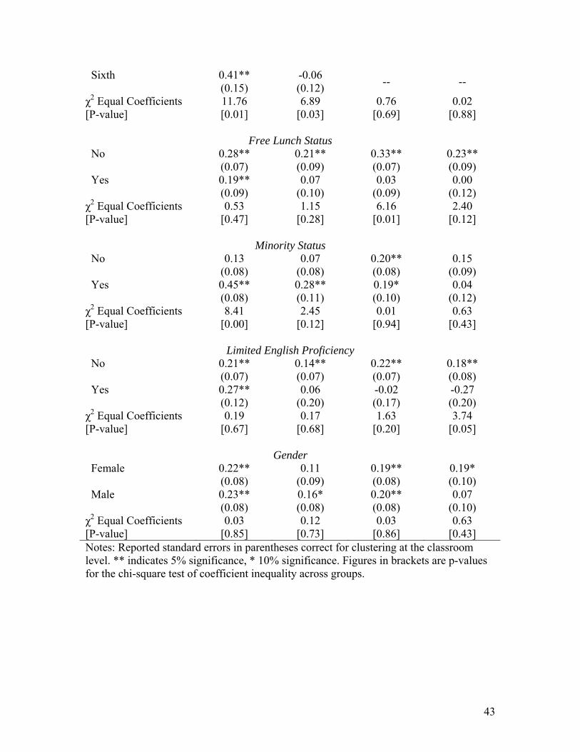
The final four panels of the table consider the heterogeneity of persistence across
groups of students with different observable characteristics. In all cases, students eligible
for free lunch had lower estimated persistence measures than ineligible students, although
the difference is only significant for one-year math scores. Although this appears to
suggest that disadvantaged students derive less persistent benefits from teacher value-
added, the following two panels suggest the true situation is much more complicated.
Minority students, for example, have a statistically significant advantage in measured
persistence for reading scores, while limited English proficient students have a negative
point estimate of persistence (although we can not reject the hypothesis of no persistence)
for teacher value-added using math scores, but no such disparity in reading. There is no
apparent pattern of differing results across gender groups.
6. Discussion
After decades of pessimism concerning the lack of connection between the
measurement of observable teacher characteristics and student achievement, the use of
value-added methods has led to renewed optimism about the ability to measure, reward

30
and provide incentives for teacher effectiveness. The primary claim of the teacher value-
added literature is that teacher quality matters a great deal for student achievement. This
claim is based on consistent findings of a large dispersion in teachers’ ability to influence
contemporary student test scores. However, our results indicate that contemporary
teacher value-added measures may overstate the ability of teachers, even exceptional
ones, to influence the ultimate level of student knowledge since they conflate variation in
short-term and long-term knowledge. Given that a school’s objective is to increase the
latter, the importance of teacher value-added measures as currently estimated may be
substantially less than the teacher value-added literature indicates. Note that this does not
mean the average level of teacher value-added is unimportant, rather that the variation in
the distribution of existing teacher value-added is less informative than contemporary test
gains suggest.
Nevertheless, our results suggest there is some long-run persistence to the gains
induced by teacher value-added, even if it is small compared to the persistence of test
score gains from all sources. Hence, it seems likely that improving teacher value-added
will improve the long-run outcomes of students. Further research comparing the
persistence of value-added with other potential educational interventions is needed to
better understand the relevant policy tradeoffs.
As discussed earlier, our statistical model will capture knowledge fadeout
stemming from a variety of different sources, ranging from poor measurement of student
knowledge to structural elements in the education system that lead to real knowledge
depreciation. Although it is impossible in the present context to definitively label one or
more explanations as verified, we can make some progress in this area. For example,
31
many of the compensatory theories suggest teachers aim to instruct at a specific,
relatively low point on their class distribution or that principals adjust class assignment to
compensate for past experiences. Our results, however, provide evidence to suggest that
these stories may be a poor fit for explaining fadeout in our district. First, we show that
controlling for the quality of the contemporary teacher does not change conclusions about
persistence. Also, there is very little correlation in our data between the value-added of
students’ lagged and twice lagged teachers such as one would expect if there were some
sort of cyclical, compensating assignment scheme. Finally, the first panel of Table 6
suggests a symmetrical relationship between student catch-up from below average
teachers and fall back from good teachers.
Another potential explanation is that the results are an artifact of test scores that
are improperly scaled. However, as mentioned above, the benchmark measures in this
paper (i.e., the OLS estimate on lagged achievement and the IV estimate on lagged
achievement that uses twice-lagged achievement as the instrument) come from the same
test scaling. Given that these measures agree with the broader literature, it does not seem
likely that scaling drives the results. In any case, the benchmarks suggest that regardless
of test mechanism, student test score changes due to teacher value-added are only one-
fifth as persistent as those due to long-run knowledge.
Should the particular explanation for fadeout change how we should think about
the policy possibilities of value-added? To examine this, consider under what
circumstances exceptional teachers could have widespread and enduring effects in ways
that belie our estimates. Three criteria would have to be met: The knowledge that
students could obtain from these exceptional teachers would have to be (1) valuable to

32
the true long-run outcomes of interest (such as wages or future happiness), (2) retained by
the student, and (3) not be tested on future exams. To the degree that all three of these
conditions exist, the implications of this analysis should be tempered.
While it is certainly possible that these conditions are all met, we believe it is
unlikely that the magnitude of fadeout we observe can be completely (or even mostly)
explained by these factors. For example, there are few instances in the mathematics of
early grades when knowledge is not cumulative. Although fourth grade exams may not
include exercises designed to measure subtraction ability, that ability is implicitly tested,
for example, in problems that require long division. Furthermore, suppose that teachers
are cheating on behalf of students or simply teaching them better techniques for specific
test items that have no general meaning outside the test. At that point, the measured
knowledge on the test is not socially valuable in some ultimate sense and a value-added
policy based on that test score should account for fadeout in the same way it would if the
fadeout was due to student forgetfulness.
7. Conclusion
In this paper, we develop a simple statistical framework to empirically assess the
persistence of treatment effects in education. We present a simple model of student
learning that incorporates permanent as well as transitory learning gains, and then
demonstrate that an intuitive and computationally simple instrumental variables estimator
can recover the persistence parameter.
The econometric framework we use to measure the persistence of teacher induced
learning gains is more broadly applicable. It can be used to the measure the persistence

33
of any educational intervention. Relative to the methods previously used, our approach
allows simple statistical inference, clear comparison across policies, and clearly relates to
the empirical results to the assumed data generating process.
Using administrative data that links teachers to student achievement scores over
multiple years, we calculate value-added measures of teacher effectiveness and use the
methods outlined above to determine the persistence of teacher effects. We find that
teacher-induced test score gains have low persistence relative to the variation in test
scores generated by all sources and the variation induced by long-run learning. Our
estimates suggest that only about one-fifth of the test score gain from a high value-added
teacher remains after a single year. Given our standard errors, we can rule out one-year
persistence rates above one-third. After two years, about one-eighth of the original gain
persists. The observed fadeout is comparable for both math and reading, and is robust to
several specification checks. Furthermore, any positive selection on observables in the
teacher-student matching process suggests that our estimates may be overly optimistic.
Previous researchers have referenced a counterfactual world in which a series of
high value-added effects for a hypothetical student with a string of good teachers may be
simply added together. Given this scenario, researchers and policymakers have
advocated the widespread use of such value-added measures in a variety of education
policies including teacher compensation and teacher/school accountability. Our results
suggest some caution should be taken in focusing on such measures of teacher
effectiveness. If value-added test score gains do not persist over time, adding up
consecutive gains does not correctly account for the benefits of higher value-added
teachers. Of course, the same caution should be attached to any educational intervention.
34
Hence, the broader implication from this work is that researchers and policymakers
should make greater effort to track the long-run impact of education policies and
programs.

References
Aaronson, Daniel, Lisa Barrow, and William Sander. (2007) Teachers and Student Achievement in the Chicago Public High Schools. Journal of Labor Economics 25 (1), 95-135. Andrabi, Tahir, Tishnu Das, Asim I. Khwaja, and Tristan Zajonc (2007) “Do Value-Added Estimates Add Value? Accounting for Learning Dynamics” mimeo. Barnett, W. S. (1985). Benefit-Cost Analysis of the Perry Preschool Program and Its Policy Implications. Educational Evaluation and Policy Analysis (7). 333-342. Boardman, A. & Murnane, R. (1979), .Using panel data to improve estimates of the determinants of educational achievement., Sociology of Education 52 (2), 113-121. Coleman, James S., et al. (1966). Equality of educational opportunity. Washington, DC: U.S. Government Printing Office. Currie, Janet., and Duncan Thomas. (1995) Does Head Start Make A Difference?, The American Economic Review 85 (3), 341-364. Doran, H. & Izumi, L. (2004). Putting Education to the Test: A Value-Added Model for California., San Francisco: Pacific Research Institute. Goldhaber, Dan D., and Dominic J. Brewer. (1997). Why don't school and teachers seem to matter? Journal of Human Resources 32, no. 3:505–23. Hanushek, Eric A. (1997). Assessing the effects of school resources on student performance: An update. Education Evaluation and Policy Analysis 19:141–64. Hanushek, Eric A. (2003), .The failure of input-based schooling policies., Economic Journal 113, 64-98. Imbens, Guido W & Angrist, Joshua D, (1994). "Identification and Estimation of Local Average Treatment Effects," Econometrica, Econometric Society, vol. 62(2), pages 467-75, March. Jacob, Brian A. and Lars Lefgren. (2008) Can Principals Identify Effective Teachers? Evidence on Subjective Performance Evaluation in Education. Journal of Labor Economics 26, 101-136.. Jacob, Brian A. and Lars Lefgren. (2007). What Do Parents Value in Education? An Empirical Investigation of Parents’ Revealed Preferences for Teachers. Quarterly Journal of Economics 122, 1603-1637.

36
Jacob, Brian A., and Lars Lefgren. (2004). Remedial Education and Student Achievement: A Regression-Discontinuity Analysis. Review of Economics and Statistics (86). 226-44. Jacob, Brian A. and Steven Levitt, (2003). Rotten Apples: An Investigation of the Prevalence and Predictors of Teacher Cheating. Quarterly Journal of Economics 118. 843-77. Kane, Thomas J., and Douglas O. Staiger. (2008). Are Teacher-Level Value-Added Estimates Biased? An Experimental Validation of Non-Experimental Estimates. Mimeo March 17. Kane, Thomas J., and Douglas O. Staiger. (2002). The promises and pitfalls of using imprecise school accountability measures. Journal of Economic Perspectives 16, no. 4:91–114. Krueger, Alan B., and Diane M. Whitmore. (2001). The Effect of Attending a Small Class in the Early Grades on College-Test Taking and Middle School Test Results: Evidence from Project STAR. Economic Journal (111). 1-28.
Lockwood, J. R., Daniel F. McCaffrey, Louis T. Mariano, and Claude Setodji. (2007) Bayesian Methods for Scalable Multivariate Value-Added Assessment. Journal of Educational and Behavioral Statistics (32). 125 - 150.
McCaffrey, Daniel F., J. R. Lockwood, Daniel Koretz, Thomas A. Louis, and Laura Hamilton (2004) “Models for Value-Added Modeling of Teacher Effects” Journal of Educational and Behavioral Statistics, Vol. 29, No. 1, Value-Added Assessment Special Issue., Spring, pp. 67-101. Nye, Barbara, Larry V. Hedges, and Spyros Konstantopoulos. (1999). The Long-Term Effects of Small Classes: A Five-Year Follow-Up of the Tennessee Class Size Experiment. Educational Evaluation and Policy Analysis (21). 127-142 Rivkin, Steven G., Eric A. Hanushek, and John F. Kain. (2005). Teachers, schools, and academic achievement. Econometrica 73, no. 2:417–58. Rockoff, Jonah E., (2004) “The impact of individual teachers on student achievement: evidence from panel data,” American Economic Review. 247-252. Rothstein, Jesse. (2007). Do Value-added Models add value? Tracking, Fixed Effects and Causal Inference. Mimeo. November 20. Sass, T. (2006). Charter schools and student achievement in Florida. Education Finance and Policy 1(1), 91-122. Todd, P. & Wolpin, K. (2003), .On the Speci.cation and Estimation of the Production Function for Cognitive Achievement., Economic Journal 113, 3-33.

37
Todd, P. & Wolpin, K. (2006), .The Production of Cognitive Achievement in Children: Home, School and Racial Test Score Gaps., Philadelphia, PA: University of Pennsylvania, PIER Working Paper pp. 4-19.

38
Table 1: Summary Statistics Variable Mean
(Std. dev.) Normalized Reading Score -0.018
(0.985)
Normalized Math Score 0.026 (0.976)
Reading Percentile Score 0.476 (0.280)
Math Percentile Score 0.489 (0.280)
Student Fraction Male 0.505 (0.500)
Student Fraction Free Lunch 0.436 (0.496)
Student Fraction Minority 0.239 (0.427)
Student Fraction Special Ed. 0.083 (0.276)
Student Fraction Limited English 0.101 (0.301)
Student Age 10.921 (1.157)
Grade 4 0.263 (0.440)
Grade 5 0.246 (0.430)
Grade 6 0.217 (0.412)
Notes: Test scores are normalized relative to the standard deviation for all students in the district.

39
Table 2: Summary of Teacher Value-added Measures Measure Mean
(Std. Dev.) Reading normalized value-added of student’s Teacher (t-1) 0.016
(0.212)
Math normalized value-added of student’s Teacher (t-1) 0.027 (0.294)
Reading normalized value-added of student’s Teacher (t-2) 0.011 (0.229)
Math normalized value-added of student’s Teacher (t-2) 0.009 (0.304)
Notes: Test scores are normalized relative to the standard deviation for all students in the district.

40
Table 3: Estimates of the One-Year Persistence of Achievement Reading Math ˆ
OLSβ ˆLRβ V̂Aβ ˆ
OLSβ ˆLRβ V̂Aβ
Prior Year Achievement Coefficient
0.66** (0.01)
0.98** (0.02)
0.22** (0.06)
0.62** (0.01)
0.98** (0.02)
0.19** (0.06)
F-Statistic of Instruments [p-value] -- 1,412
[0.00] 48
[0.00] -- 839 [0.00]
65 [0.00]
Observations 18,240 18,240 18,240 14,182 14,182 14,182 R-Squared 0.59 0.51 0.44 0.51 0.41 0.36 Notes: Reported standard errors in parentheses correct for clustering at the classroom level. ** indicates 5% significance, * 10% significance. Table 4: Estimates of the Two-Year Persistence of Achievement Reading Math ˆ
OLSβ ˆLRβ V̂Aβ ˆ
OLSβ ˆLRβ V̂Aβ
Two Year Prior Achievement Coefficient
0.60** (0.01)
0.95** (0.03)
0.13** (0.06)
0.59** (0.02)
0.97** (0.04)
0.13 (0.08)
F-Statistic of Instruments [p-value] -- 961
[0.00] 55
[0.00] -- 439 [0.00]
63 [0.00]
Observations 10,216 10,216 10,216 7,104 7,104 7,104 R-Squared 0.54 0.44 0.36 0.49 0.37 0.31 Notes: Reported standard errors in parentheses correct for clustering at the classroom level. ** indicates 5% significance, * 10% significance.

41
Table 5: Robustness Checks Reading Math 1 Year
Persistence 2 Year
Persistence 1 Year
Persistence 2 Year
Persistence
(1) Baseline 0.22** (0.06)
0.13** (0.06)
0.19** (0.06)
0.13 (0.08)
(2) Controlling Only for Grade, School, and Year in Second Stage
0.32** (0.06)
0.23** (0.06)
0.22** (0.06)
0.19** (0.08)
(3) Controlling for Classroom Fixed Effects in Second Stage
0.19** (0.05)
0.14** (0.06)
0.12** (0.05)
0.11* (0.07)
(4) Value-Added Estimated Using Achievement Gains
0.15** (0.07)
0.11 (0.07)
0.08 (0.07)
0.08 (0.09)
(5) Value-Added Estimated Using Achievement Gains Normalized by Initial Score
0.16** (0.06)
0.10 (0.07)
0.16** (0.07)
0.14* (0.08)
(6) Value-Added Estimated Using Students in Middle of Achievement Distribution
0.15** (0.07)
0.14** (0.06)
0.18** (0.07)
0.24** (0.08)
(7) Test Performance Measured in Percentiles of District Performance
0.17** (0.07)
0.14** (0.05)
0.18** (0.05)
0.14** (0.06)
Notes: Reported standard errors in parentheses correct for clustering at the classroom level. ** indicates 5% significance, * 10% significance.

42
Table 6: Heterogeneity of Persistence of Teacher Induced Achievement Reading Math 1 Year
Persistence 2 Year
Persistence 1 Year
Persistence 2 Year
Persistence Baseline 0.22**
(0.06) 0.13** (0.06)
0.19** (0.06)
0.13 (0.08)
Positive vs. Negative Teacher Shocks
Top Third of Teacher Quality Compared to Middle Third
0.16 (0.12)
0.21 (0.13)
0.15 (0.21)
0.15 (0.14)
Bottom Third of Teacher Quality Compared to Middle Third
0.42 (0.16)
0.10 (0.20)
0.15 (0.10)
0.14 (0.17)
χ2 Equal Coefficients [P-value]
0.99 [0.32]
0.16 [0.69]
0.00 [0.99]
0.00 [0.98]
Year
1999 0.33** (0.10) -- 0.39**
(0.08) --
2000 -0.08 (0.18)
0.30** (0.14)
-0.21 (0.19)
0.25** (0.10)
2001 0.13 (0.10)
0.00 (0.17)
0.08 (0.13)
0.00 (0.14)
2002 0.31** (0.14)
0.15 (0.10)
0.01 (0.13)
0.16 (0.15)
2003 0.30** (0.12)
0.07 (0.19)
0.32** (0.09)
0.13 (0.15)
2004 0.47** (0.12)
0.16 (0.13)
0.32** (0.14)
0.27** (0.13)
2005 0.37** (0.15)
0.16 (0.17)
0.41** (0.13)
0.02 (0.22)
χ2 Equal Coefficients [P-value]
9.22 [0.16]
2.07 [0.84]
15.23 [0.02]
3.46 [0.63]
Grade
Third 0.14 (0.12) -- 0.18
(0.13) --
Fourth 0.38** (0.09)
0.08 (0.16)
0.23** (0.08)
0.14 (0.13)
Fifth -0.19 (0.16)
0.28** (0.07)
0.06 (0.18)
0.12 (0.09)
43
Sixth 0.41** (0.15)
-0.06 (0.12) -- --
χ2 Equal Coefficients [P-value]
11.76 [0.01]
6.89 [0.03]
0.76 [0.69]
0.02 [0.88]
Free Lunch Status
No 0.28** (0.07)
0.21** (0.09)
0.33** (0.07)
0.23** (0.09)
Yes 0.19** (0.09)
0.07 (0.10)
0.03 (0.09)
0.00 (0.12)
χ2 Equal Coefficients [P-value]
0.53 [0.47]
1.15 [0.28]
6.16 [0.01]
2.40 [0.12]
Minority Status
No 0.13 (0.08)
0.07 (0.08)
0.20** (0.08)
0.15 (0.09)
Yes 0.45** (0.08)
0.28** (0.11)
0.19* (0.10)
0.04 (0.12)
χ2 Equal Coefficients [P-value]
8.41 [0.00]
2.45 [0.12]
0.01 [0.94]
0.63 [0.43]
Limited English Proficiency
No 0.21** (0.07)
0.14** (0.07)
0.22** (0.07)
0.18** (0.08)
Yes 0.27** (0.12)
0.06 (0.20)
-0.02 (0.17)
-0.27 (0.20)
χ2 Equal Coefficients [P-value]
0.19 [0.67]
0.17 [0.68]
1.63 [0.20]
3.74 [0.05]
Gender
Female 0.22** (0.08)
0.11 (0.09)
0.19** (0.08)
0.19* (0.10)
Male 0.23** (0.08)
0.16* (0.08)
0.20** (0.08)
0.07 (0.10)
χ2 Equal Coefficients [P-value]
0.03 [0.85]
0.12 [0.73]
0.03 [0.86]
0.63 [0.43]
Notes: Reported standard errors in parentheses correct for clustering at the classroom level. ** indicates 5% significance, * 10% significance. Figures in brackets are p-values for the chi-square test of coefficient inequality across groups.