the physics of magnetic resonance imaging fys … physics of magnetic resonance imaging fys-kjm 4740...
TRANSCRIPT

The Physics of Magnetic Resonance Imaging
FYS-KJM 4740
Atle Bjørnerud Department of Physics
University of Oslo March 2008

FYS-KJM 4740 - The Physics of MRI 2
Preface I (2006) Magnetic Resonance Imaging (MRI) is probably the most powerful medical imaging technology today, combining great versatility with superb contras resolution. It is probably also the most demanding and challenging modality from a physics point of view. It is therefore a challenging and daunting task to attempt to give a ‘complete’ overview of the field of MR physics in a one-term course. In fact, this is not possible and some priorities have to be made about what to include and what to leave out. This compendium is the result of such a selection process where I have tried to cover the basic physics of MRI within the areas I believe are most important to get started as a researcher in the MR-field. Some important topics are still missing which should really have been included; especially related to hardware, coil design and parallel imaging techniques. Hopefully these topics will be better covered in a future revision. The compendium is, to a large extent based on the excellent textbook by Vlaardingerbroek and den Boer, but I have also used many other sources of information. I have included all relevant literature sources in a ‘Further Reading’ list at the end of each chapter. Most of the figures related to dynamic magnetisation behaviour are based on self-made simulations (from the Bloch equations) since I often had to convince myself that the theory made sense in reality… I would like to acknowledge Sven Månsson (Malmø) for letting me use some of his figures and extracts from a book chapter we wrote together some years ago. Also, thanks to Kyrre Eeg Emblem and Oliver Geier at Rikshospitalet Univ. Hosp and Arvid Morell and Lars Johansson at Uppsala Univ. Hosp for providing some of the MR images used in the compendium. Enjoy!
Oslo, 15 March 2006
Atle Bjørnerud

FYS-KJM 4740 - The Physics of MRI 3
Preface II (2008) Have now added chapters on Contrast agents (theory and advanced applications)
as well as diffusion weighted imaging (DWI, DTI). Further, several figures have been modified and a fair amount of spelling mistakes and other errors have been corrected (probably still some left so please let me know whenever you spot errors in the text!)
Oslo, May 2008 Atle Bjørnerud

FYS-KJM 4740 - The Physics of MRI 4
1. The Bloch equation, excitation and relaxation ........................................................... 7
1.1. Introduction .......................................................................................................... 7
1.2. Non-selective RF excitation ................................................................................. 8
1.3. Relaxation........................................................................................................... 13
1.3.1. T1 relaxation ............................................................................................... 13
1.3.2. T2 relaxation ............................................................................................... 14
1.3.3. Relaxation and MR signal behaviour .......................................................... 15
1.4. Further reading – Chapter 1 ............................................................................... 17
2. Image Formation ....................................................................................................... 18
2.1. Slice-selective RF excitation .............................................................................. 18
2.2. The k-space ........................................................................................................ 22
2.3. Effects of discrete sampling ............................................................................... 27
2.4. Further reading – Chapter 2 ............................................................................... 32
3. Pulse sequences – an introduction ............................................................................ 33
3.1. The Gradient Echo (GRE) sequence .................................................................. 34
3.2. The Spin Echo (SE) sequence ............................................................................ 37
4. MR signal behaviour and image contrast.................................................................. 39
4.1. Spin Echo signal behaviour ................................................................................ 39
4.2. T1-weighted (Spoiled) Gradient Echo signal behaviour .................................... 44
4.3. Multi-slice and 3D acquisitions.......................................................................... 50
4.3.1. 2D multi-slice acquisitions ......................................................................... 50
4.3.2. 3D acquisitions............................................................................................ 51
4.4. Further reading – Chapter 4 ............................................................................... 53
5. Steady state sequences .............................................................................................. 54
5.1. Eight-ball echo ................................................................................................... 54
5.2. Stimulated echo .................................................................................................. 55
5.3. Steady state signal behaviour ............................................................................. 58
5.4. Steady state GRE sequences .............................................................................. 62
5.4.1. Large net-gradient surface .......................................................................... 64
5.4.2. Balanced GRE – TrueFISP ......................................................................... 65
5.4.3. T1-GRE – Spoiled GRE.............................................................................. 68
5.1. Transient signal response ................................................................................... 70
5.2. Further reading – Chapter 5 ............................................................................... 72
6. Accelerated k-space trajectories ............................................................................... 73
6.1. Fast Spin Echo (FSE) ......................................................................................... 74
6.2. Echo Planar imaging (EPI) ................................................................................. 81
6.2.1. Artifacts in EPI sequences .......................................................................... 82
6.3. Spiral imaging .................................................................................................... 86
6.4. Further reading – Chapter 6 ............................................................................... 87
7. Magnetisation preparation ........................................................................................ 88
7.1. Selective tissue suppression ............................................................................... 91
7.2. Influence of excitation pulses on the magnetization curve ................................ 92
8. Image quality, signal, contrast and noise .................................................................. 94
8.1. Signal versus noise ............................................................................................. 94
8.2. Signal versus contrast ......................................................................................... 96
8.3. Practical measurements of SNR and CNR ......................................................... 98

FYS-KJM 4740 - The Physics of MRI 5
8.4. Partial k-space sampling................................................................................... 101
8.4.1. Partial echo acquisition ............................................................................. 101
8.4.2. Reduced matrix acquisition....................................................................... 102
8.5. Further reading – Chapter 8 ............................................................................. 103
9. Off-resonance effects .............................................................................................. 104
9.1. Magnetic susceptibility .................................................................................... 104
9.1.1. Diamagnetism ........................................................................................... 105
9.1.2. Paramagnetism .......................................................................................... 106
9.2. Implications for imaging .................................................................................. 106
9.2.1. Intravoxel dephasing – signal loss ............................................................ 107
9.2.2. Off-resonance effects – geometric distortions .......................................... 109
9.2.3. Water-fat shift ........................................................................................... 114
9.3. Further reading – Chapter 9 ............................................................................. 116
10. Spins in motion .................................................................................................... 117
10.1. Phase dispersion due to flow ........................................................................ 117
10.2. Flow compensation ....................................................................................... 119
10.3. Flow artifacts ................................................................................................ 122
10.3.1. Flow voids ............................................................................................. 122
10.3.2. Misregistration ...................................................................................... 122
10.3.3. Effects of pulsatile flow ........................................................................ 125
10.4. Further reading – Chapter 10 ........................................................................ 126
11. MR Contrast Agents ............................................................................................ 127
11.1. Classification of MR contrast agents ............................................................ 127
11.1.1. Magnetic properties ............................................................................... 127
11.1.2. Biodistribution ....................................................................................... 129
11.1.3. Image enhancement ............................................................................... 129
11.2. Contrast agent relaxivity ............................................................................... 130
11.3. In vivo relaxivity and MR contrast enhancement ......................................... 132
11.3.1. Dipolar relaxation .................................................................................. 132
11.3.2. Water exchange effects ......................................................................... 135
11.3.3. Susceptibility induced relaxation. ......................................................... 138
11.4. Further reading Chapter 11 ........................................................................... 143
12. Advanced Applications of MR Contrast Agents ................................................. 144
12.1. T1-based dynamic imaging ........................................................................... 144
12.2. T2/T2* based dynamic imaging ................................................................... 145
12.3. Perfusion imaging ......................................................................................... 146
12.4. Dynamic contrast enhanced imaging ............................................................ 150
13. MR Angiography ................................................................................................. 153
13.1. Time-of-flight (TOF) MRA. ......................................................................... 153
13.2. Maximum Intensity Projection (MIP) .......................................................... 156
13.3. 3D-TOF techniques ...................................................................................... 156
13.4. Artery / vein selection – use of saturation slabs. .......................................... 158
13.5. Contrast enhanced MRA .............................................................................. 159
13.6. Further reading – Chapter 13 ........................................................................ 160
14. Imaging Water Diffusion ..................................................................................... 161
14.1. Molecular diffusion ...................................................................................... 161

FYS-KJM 4740 - The Physics of MRI 6
14.2. Diffusion weighted imaging ......................................................................... 163
14.3. Imaging Diffusion Anisotropy...................................................................... 167
14.3.1. Rotationally invariant diffusion indices ................................................ 173
14.3.2. Diffusion tractography .......................................................................... 175
14.4. Further reading – Chapter 12 ........................................................................ 177
15. Imaging Hardware ............................................................................................... 178
15.1. The magnet ................................................................................................... 178
15.2. RF-electronics ............................................................................................... 178
15.3. Further reading – Chapter 15 ........................................................................ 180

FYS-KJM 4740 - The Physics of MRI 7
1. The Bloch equation, excitation and relaxation
1.1. Introduction
Magnetic Resonance Imaging (MRI) is based on the discovery, made more than
50 years ago (Bloch and Purcell), that nuclei with a spin angular momentum (spin) can interact with a magnetic field. The essence of this interaction, known as nuclear magnetic resonance (NMR) is described by the simple linear relationship between the static magnetic flux density (magnetic field) B0 experienced by a nuclei and the resulting angular frequency of rotation ω0 of the nuclear spin:
Eq. 1-1
00 Bγω =
where γ is the gyromagnetic ratio, which is a unique constant for each nuclear isotope possessing a spin. All current clinical use of MRI (not including spectroscopy) is based on proton NMR (with spin ½) and for protons γ/2π= 42.6 x 10⁶ Hz/Tesla. The angular frequency ω0 is referred to as the Larmor frequency, and is identical to the frequency of the electromagnetic radiation associated with possible spin energy transitions induced by the magnetic field B0. Although the NMR phenomenon is purely a quantum mechanical process, its macroscopic manifestation is, under most circumstances, well described by classical physics. For a population of nuclei with a spin quantum number of I, and thus 2I + 1 energy states, the distribution of the spins in each state is, in thermal equilibrium, governed by the Boltzmann law, as follows:
Eq. 1-2
∑=
−=
−
−=
In
In
Bn
Bmm
TkE
TkE
N
N
))/(exp(
))/(exp(
0
where Nm is the number of spins in the state m, N0 is the total number of spins, Em is the energy of state m, T is the absolute temperature and kB is the Boltzmann constant.
Each nuclear spin is associated with a dipolar magnetic moment µµµµ1. In fact, in the very first description of NMR the effect was used to accurately measure nuclear magnetic moment (Rabi). The nuclear magnetic moment can be thought of as the magnetic energy per unit magnetic flux density induced by the current loop associated with the rotation, due to B0, of the charged protons in a nucleus. Although the current loop of a single proton is negligible and has almost zero dimension, the sum of the individual magnetic moments of all the protons contained in a macroscopic sample is finite (there are of the order of 1022 protons/cm3 living tissue) and is referred to as the macroscopic
magnetization of the sample, M = ∑µµµµ. In a sample in equilibrium state, the precession of an individual spin around the B0-field will not be coherent with other spins, causing the
1 Vectors and matrices will be denoted by bold typeface

FYS-KJM 4740 - The Physics of MRI 8
component of M in the x-y plane (perpendicular to B0) to be zero. However, the z-component of an individual spin µz is restricted to discrete values µz= γmIħ, with mI=-I, -I+1, …. I. Using the approximation ex≈1+x for small x, and summing the z-contribution to M for each m-state, we obtain the following expression for Mz :
Eq. 1-3
0Z BMTk
IIN
B3
)1(22
0 +=
hγ
Eq. 1-3 is known as Curie’s law, and expresses some important relationships:
• Mz is directly proportional to the magnetic field strength B0. Hence, higher field strength gives a larger MR-signal.
• Mz is proportional to γ2. 1H has the highest value of γ of all isotopes present in vivo and the large γ combined with the high abundance of water in tissue makes protons by far the most detectable nuclei in clinical MRI.
For protons (with I=1/2) the spins are distributed in only two states (spin ‘up’ = low energy and spin ‘down’ = high energy) and the two populations, N+ and N- are then related by the following (using ∆E = γħB0):
Eq. 1-4
))/(exp( 0 TkBN
NBhγ=
−
+
Example: for a magnetic field strength of 1.5 T, at room temperature (300 K), the ratio N+/N- will, for protons (γ = 2.68 x 10⁸ s-1 T-1) be 1 + 1.02 x 10⁻⁵. I.e. there is only about 1 proton out of every 105 protons which contribute to the macroscopic magnetization, M, at 1.5 Tesla.
1.2. Non-selective RF excitation
The behavior of the macroscopic magnetization vector as a result of magnetic
interactions is described classically by the Bloch equation:
Eq. 1-5
)( BMM
×= γdt
d

FYS-KJM 4740 - The Physics of MRI 9
Eq. 1-5 states that the vector describing the rate of change of M is perpendicular to both B and M. In other words, the macroscopic magnetisation vector M precesses about the direction of the magnetic field – in analogy to the precession of a gyroscope about the gravitational field (Figure 1-1). When the spin system is in a state of equilibrium the net magnetisation points in the direction of the main magnetic field, referred to as the z-direction with a magnitude given by Mz (since the x- and y- components of M average out). MRI is based on the detection of the magnetisation vector M. However, in order to
get any information about M, the vector needs to be moved away from its equilibrium orientation parallel to B0. Further, M needs to oscillate in time in order to induce a current in a coil. This is achieved by applying a second magnetic field, B1, perpendicular to B0. The motion of the magnetisation vector in the presence of both the B0 and B1 fields can then be written as:
Eq. 1-6
)( 10 BBMM
+×= γdt
d
The linearly oscillating B1-vector can be re-written as the sum of two rotating vectors, B1
+ and B1- rotating in opposite directions (Figure 1-3). B1
+ rotates clockwise with an angular frequency –Ω, and the other rotating counter-clockwise with an angular frequency +Ω:
z
y
x
B0
M
ωL
Mz
ωL
Figure 1-1. The magnetic moment M rotates around the static B-field at the Larmor frequency

FYS-KJM 4740 - The Physics of MRI 10
Eq. 1-7
Ω
=
Ω
Ω
+
Ω−
Ω−
=+= −+
0
0
)cos(
2
0
)sin(
)cos(
0
)sin(
)cos(
111111
t
Bt
t
Bt
t
BBBB
To describe the motion of the macroscopic magnetization M, it is helpful to
introduce a new Cartesian coordinate system (x’, y’, z’) rotating around the z-axis of the fixed (x, y, z) system with an angular velocity -Ω; i.e. a coordinate system which follows the rotating B1+-vector (see Figure 1-4). These two coordinate systems are called the ‘laboratory frame’ (x, y, z) and the ‘rotating frame’ (x’, y’, z’), respectively. When viewed from a rotating frame, B1+ will appear static whereas B1- will rotate with an angular velocity of 2Ω.
It can thus be shown that the rate of change of M in the rotating frame is given by:
z
y
x
B1
B1+ B1-
-Ω Ω
2B1cos(Ωt)
Figure 1-2. The RF-coil generates a magnetic field B1 along the x-axis
Figure 1-3. The oscillating B1-field as the vector sum of two fields rotating in opposite directions.

FYS-KJM 4740 - The Physics of MRI 11
Eq. 1-8
effBMM
×= γdt
d
where Beff is the effective field given by B0 + B1 + Ω/γ. Note that the vectors Ω and B0 have opposite directions (Figure 1-4):
Eq. 1-9
Ω−
= 0
0
Ω
If Ω= γB0 (i.e. the frequency of the B1 field = the Larmor frequency), the effective field consists only of the B1-field, which in turn is composed of the static B1+ -field and the rotating B1- -field. The rotating B1- -field has negligible influence on M when averaged over time, and the net effect of applying the RF-field, B1, is therefore a precession of M around the B1+, with an angular velocity given by:
Eq. 1-10
11 Bγω −=
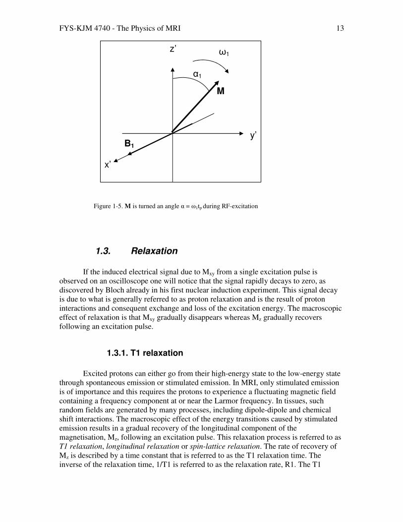
If the B1-field is turned on during the time tp, M will rotate an angle α = ω1tp from its position at t=0 down towards the x’y’-plane. The angle α is called the ‘flip angle’ of the RF-pulse (see Figure 1-5).
We have now seen that during, and immediately after the application of an RF-pulse along the x- (or y-) axis, there will be a component of M present in the xy-plane, Mxy that rotates about the z-axis. The oscillating nature of Mxy makes it possible to detect the presence of this magnetisation component through the induction of a current in a coil placed within the oscillating field. The observed signal due to Mxy is referred to as the MR signal or the free induction decay (FID). Note that Mz is not detectable because it does not rotate and hence does not induce a current. The term decay refers to the fact the

FYS-KJM 4740 - The Physics of MRI 12
signal rapidly disappears due to proton relaxation processes, as discussed further below. The effect of applying an RF-pulse along the x’-axis can also be expressed in matrix notation as follows:
Eq. 1-11
−
=
z
y
x
x
x
M
M
M
B
Bdt
d
00
00
000
1
1γM
This differential equation can readily be solved by eliminating the Mz-term to obtain:
Eq. 1-12
)cos()sin( '1'1' tBBtBAM xxy γγ +=
Using the boundary conditions My’=My’(0) and Mz’=Mz(0) at t=0, we get:
Eq. 1-13
0
11
11
)0(
)0(
)0(
)cos()sin(0
)sin()cos(0
001
)( MRM ⋅=
−
=
z
y
x
M
M
M
tt
ttt
ωω
ωω
The RF-excitation process can therefore be thought of as a applying a rotation matrix R around the x’-axis as shown in Figure 1-5.
z
y
x y’
z’
x’
Ω
Ω
Figure 1-4. The ‘rotating frame’ (x’, y’, z’-coordinates)
FYS-KJM 4740 - The Physics of MRI 13
1.3. Relaxation
If the induced electrical signal due to Mxy from a single excitation pulse is
observed on an oscilloscope one will notice that the signal rapidly decays to zero, as discovered by Bloch already in his first nuclear induction experiment. This signal decay is due to what is generally referred to as proton relaxation and is the result of proton interactions and consequent exchange and loss of the excitation energy. The macroscopic effect of relaxation is that Mxy gradually disappears whereas Mz gradually recovers following an excitation pulse.
1.3.1. T1 relaxation
Excited protons can either go from their high-energy state to the low-energy state through spontaneous emission or stimulated emission. In MRI, only stimulated emission is of importance and this requires the protons to experience a fluctuating magnetic field containing a frequency component at or near the Larmor frequency. In tissues, such random fields are generated by many processes, including dipole-dipole and chemical shift interactions. The macroscopic effect of the energy transitions caused by stimulated emission results in a gradual recovery of the longitudinal component of the magnetisation, Mz, following an excitation pulse. This relaxation process is referred to as T1 relaxation, longitudinal relaxation or spin-lattice relaxation. The rate of recovery of Mz is described by a time constant that is referred to as the T1 relaxation time. The inverse of the relaxation time, 1/T1 is referred to as the relaxation rate, R1. The T1
Figure 1-5. M is turned an angle α = ω1tp during RF-excitation
z’
y’
x’
B1
α1
M
ω1

FYS-KJM 4740 - The Physics of MRI 14
relaxation times in different tissues vary from several seconds in body fluids like cerebrospinal fluid to less than 300 ms in fat, and these differences in T1 give rise to the image contrast when using pulse sequences which are sensitive to variations in T1 relaxation times; referred to as T1-weighted sequences. In T1-weighted sequences, TR is short (compared to the longest T1 to be observed) and tissues with a short T1 will then give more signal than tissues with a long T1 since more magnetization is recovered in the TR-interval.
1.3.2. T2 relaxation
The term T2 relaxation is used to describe the decay of the transverse component of the magnetisation, Mxy, following an excitation pulse. This time constant is also referred to as the transverse- or spin-spin relaxation time (and the corresponding relaxation rate 1/T2=R2). One might expect from the discussion of T1-relaxation above that the transverse component of the magnetisation will decay at the same rate as Mz is recovered so that T1=T2. However, in any medium (except pure water) the decay of Mxy
occurs significantly faster than the recovery of Mz due to additional relaxation effects affecting the net magnetisation in the transverse plane. T2 relaxation is caused by local field inhomogeneities on a microscopic scale. These field variations are introduced by various ‘shielding effects’ at the molecular level as well as macroscopic field inhomogeneities in the field due to variations in the local susceptibility. Immediately following an excitation pulse all the protons in a voxel precess in phase and their individual magnetic moments will collectively contribute to the transverse magnetisation vector. However, the presence of field variations on a molecular level will introduce variations in the Larmor frequency with consequent loss of phase coherence among the spins in a voxel. The loss of phase coherence therefore causes Mxy to decay faster than Mz is recovering so that T2 is always shorter than T1 in vivo. Transverse relaxation times in vivo can vary significantly depending on tissue composition and local field homogeneity and T2 is generally longer in fluids than in solid tissues. Changes in T2 relaxation times are therefore in many instances a sensitive marker for tissue pathology because many pathological processes are associated with changes in the tissue water content. The spins will also dephase if there are bulk inhomogeneities in the B0-field (which is always the case), and the actual T2 decay rate is commonly referred to as T2* rather than T2 to include the effect of bulk inhomogeneities as described by:
Eq. 1-14
02
1
*2
1B
TT∆+= γ
where ∆B0 should be interpreted as the bulk inhomogeneity within a single volume element (voxel) in the final image. Note that an important component of ∆B0 is generated by inhomogeneities due to susceptibility differences between different tissue types and at interfaces between tissue and air. This will be discussed in more detail in Chapter 9.

FYS-KJM 4740 - The Physics of MRI 15
1.3.3. Relaxation and MR signal behaviour
The relaxation process can, with good accuracy, by described by the following three differential equations:
Eq. 1-15
2T
M
dt
dM xx −= ,
2T
M
dt
dM yy−= ,
1
0
T
MM
dt
dM zz −−=
where M0 is the equilibrium magnetization along the z-axis given by Eq. 1-3. In the presence of relaxation, the Bloch equation can be expressed as:
Eq. 1-16
)( 0MMRBMM
−−×= effdt
dγ
where
Eq. 1-17
=
1
2
2
100
01
0
001
T
T
T
R and
=
0
0 0
0
M
M ,
=
z
y
x
M
M
M
M
and Beff is the effective field (Eq. 1-8) and M0 is the equilibrium magnetisation. Since we assume that relaxation effects can be neglected during RF-excitation the effects of relaxation on the magnetization components can be obtained by solving the differential equations in Eq. 1-16 which gives:
Eq. 1-18
( )[ ] ( )110 /exp)0(/exp1)( TtMTtMtM zz −+−−=
Eq. 1-19
)/exp()0()( 2TtMtM xyxy −=

FYS-KJM 4740 - The Physics of MRI 16
Eq. 1-18 and Eq. 1-19 form an important basis for all calculations of signal behaviour in MRI. Figure 1-6 shows the evolution of the transverse (Mxy) and longitudinal (Mz) magnetization components after the application of an RF excitation pulse. Mz returns to the equilibrium magnetization with the time-constant T1 whereas Mxy decays with a time-constant T2*. Since it is the Mxy magnetization component which actually generates the MR signal, the decaying signal following the excitation pulse is commonly referred to as the ‘free induction decay’ (FID) signal. Note that the T2*-relaxation is faster than the T2-relaxation due to the field inhomogeneity term in Eq. 1-14.
From the above, the influence of the T1-relaxation on the MR signal behaviour becomes evident. Any MR imaging experiment consists of a large train on RF-pulses applied in a sequence – called a pulse sequence (as discussed in Chapter 3) and the effect of Mz following a given RF-pulse will depend on the previous magnetization history. Take, for instance, a train of 90o pulses. After the first RF-pulse, the entire equilibrium magnetization M0 will be turned into the x-y-plane. However, if the next RF-pulse is applied before the longitudinal magnetization component, Mz, has completely recovered, then Mxy following the next RF-pulse will depend on the T1-relaxation time and will generally be smaller than the full magnetization. Further, if the interval between successive RF-pulses (called the repetition time, TR) is short compared to the T2-relaxation time, then the remnant Mxy magnetization following the first RF-pulse, will the be flipped down towards the –z-axis by the next RF-pulse. After a certain number of RF-pulses, a steady-state situation is established whereby Mz and Mxy have the same magnitude after each new excitation as shown in Figure 1-7.
t
Mz
RF- pulse
T1-relaxation
t
Mxy
RF- pulse
T2* (FID)
T2-relaxation
M0
t
Mz
RF- pulse
T1-relaxation
t
Mxy
RF- pulse
T2* (FID)
T2-relaxation
t
Mz
RF- pulse
T1-relaxation
t
Mz
RF- pulse
T1-relaxation
t
Mxy
RF- pulse
T2* (FID)
T2-relaxation
t
Mxy
RF- pulse
T2* (FID)
T2-relaxation
M0
Figure 1-6. The T1- and T2 -relaxation processes following an excitation pulse.

FYS-KJM 4740 - The Physics of MRI 17
From the Bloch equation including effects or relaxation and excitation, the ‘steady-state’ signal behavior of any pulse sequence can in theory be calculated by solving Eq. 1-16 for a given experiment.
There are two important timing parameters in all pulse sequences; the repetition
time (TR) and the echo time (TE). TR describes the time-interval between successive RF-excitations in a pulse sequence and TE describes the time delay from the excitation pulse and the actual read-out (recording) of the signal. For now we state (somewhat over-simplified) that the repetition time determines the influence of T1-relaxation on the signal (through the term exp(-TR/T1) whereas the echo time determines the influence of T2-relaxation on the signal (through the term exp(-TE/T2). This will be discussed in more detail in Chapter 4.
1.4. Further reading – Chapter 1
1. Pedersen B. and Hansen E.W. Nuclear magnetic resonance. Compendium. UiO
February 2006. 2. Bloch F. Nuclear induction. Phys Rev 1946;70:460-474. 3. Purcell EM, Torrey HC, Pound RV. Resonance absorption by nuclear magnetic
moments in solid. Phys Rev 1946;69:37-38. 4. Rabi II, Zacharias JR, Millman S, Kusch P. New method of measuring nuclear
magnetic moment (letter). Phys Rev 1938;53:318-318. 5. Månsson S, Bjornerud A. Physical principles of medical imaging by nuclear
magnetic resonance. In: Merbach AE and Toth E, editors. The chemistry of contrast agents in medical magnetic resonance imaging. Chichester: Wiley; 2001. p 1-43.
0.1
0.15
0.2
0.25
0.3
0.35
0.4
0.45
0.5
0.55
1 6 11 16 21 26 31
Number of RF pulses
Mx
y+
Spoiled
Steady state (spoiled)
Figure 1-7. The progression of the Mxy (in relative units) towards a steady state level following multiple RF-pulses.

FYS-KJM 4740 - The Physics of MRI 18
2. Image Formation
So far, we have discussed the macroscopic magnetization behaviour in response to RF-excitation pulses We have seen how the Bloch equation forms the basis for all calculations of magnetization (and hence MR signal) behaviour in MRI. We shall now look in more detail on how an MR image is generated from multiple RF-excitation pulses.
2.1. Slice-selective RF excitation
In most imaging situations we are not interested in exciting the entire object (e.g.
patient) at once. In order to make an image, the excitation needs to be selective to a small part of the body; e.g. a thin slice through the head or the abdomen. In order to achieve this, the RF-excitation pulse needs to be selective in the sense that it only affects protons in a defined plane though the body. This selectivity is achieved by introducing magnetic field gradients which causes the Larmor frequency to be a function of position. Applying the gradient along the z-direction the effective field strength now becomes:
Eq. 2-1
rGBB 0z )(t(t) +=
where r is the position vector and G is the gradient strength (in mT/m). A gradient applied during RF-excitation is referred to as a ‘slice selective gradient’. The effective field strength can now be expressed as:
Eq. 2-2
Ω−+
=++⋅+=
γ
γ10
1
0
zGB
B
z
ΩBrGBB 10eff
From Eq. 2-2 it can be seen that, by making Ω=γ(B0 + Gz∆z), the effective field at z=z1 is:
Eq. 2-3
=
0
0
1B
effB
That is, the effective field is entirely in the x’-direction and M’ will therefore rotate around the x’-axis towards the x’-y’ plane. If, on the other hand B0 + Gz∆z –Ω/γ >> B1
FYS-KJM 4740 - The Physics of MRI 19
then Beff will be effectively parallel to the z’-axis and M’ will remain close to its original position; i.e. the magnetization is unaffected by the RF-pulse. Thus, it is possible to create transversal magnetization in a selected slice without significantly effecting spins outside a given interval. The position of the excited slice can be adjusted by either adjusting the frequency Ω of the RF-pulse or the strength of the gradient Gz. The thickness of the excited slice (called slice thickness) can be adjusted by adjustment of the bandwidth of the RF-pulse. The slice thickness is also affected by the strength of gradient with a given bandwidth. So far, we have assumed that the excitation pulse contains a single frequency, Ω. In practice (for a pulse of finite duration), the B1-field has a finite bandwidth ∆ω, and the slice thickness is therefore given by
Eq. 2-4
)/( zGz γω∆=∆
Thus, the slice can be made thinner by either increasing Gz or decreasing ∆ω (by increasing the RF-pulse duration). Note that, although in this example we assumed the excited slice to be perpendicular to the z-axis, the slice can be chosen arbitrarily by using combinations of the z-, y- and z- gradients.
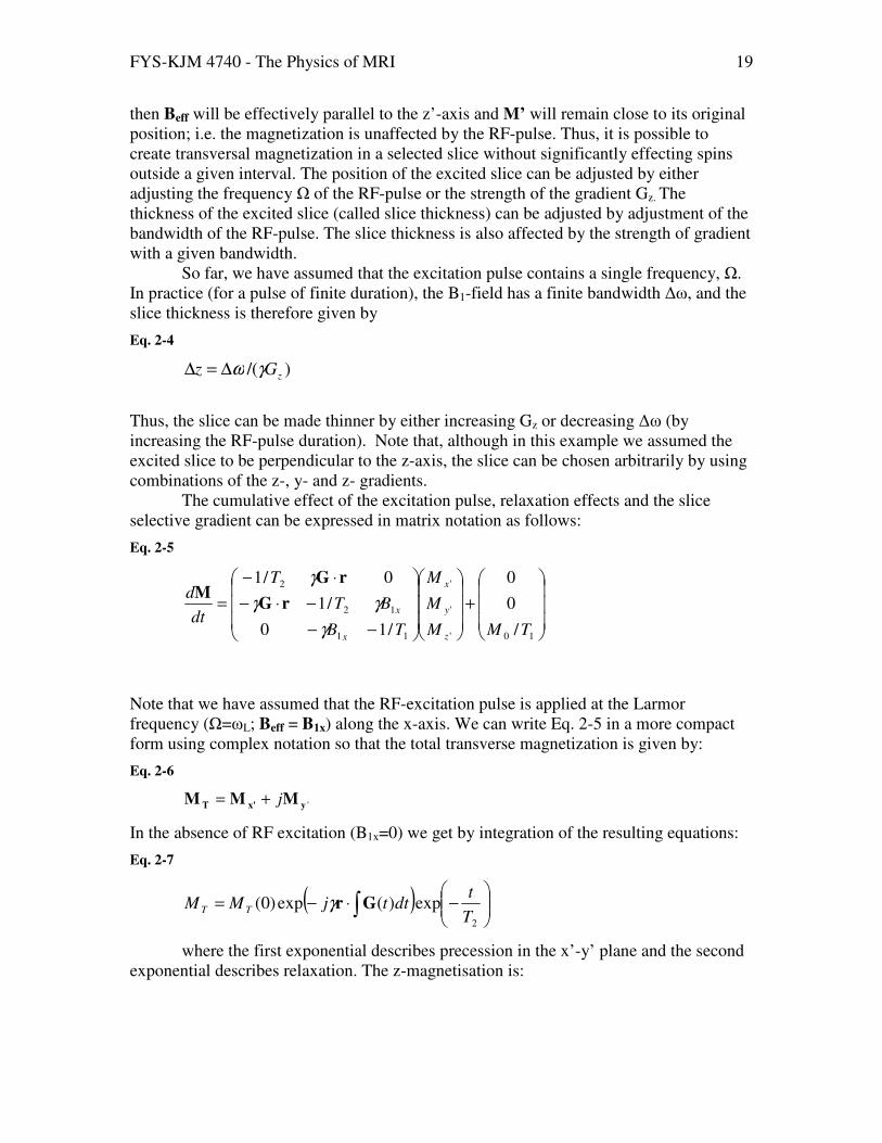
The cumulative effect of the excitation pulse, relaxation effects and the slice selective gradient can be expressed in matrix notation as follows:
Eq. 2-5
+
−−
−⋅−
⋅−
=
10'
'
'
11
12
2
/
0
0
/10
/1
0/1
TMM
M
M
TB
BT
T
dt
d
z
y
x
x
x
γ
γγ
γ
rG
rGM
Note that we have assumed that the RF-excitation pulse is applied at the Larmor frequency (Ω=ωL; Beff = B1x) along the x-axis. We can write Eq. 2-5 in a more compact form using complex notation so that the total transverse magnetization is given by:
Eq. 2-6
'yx'T MMM j+=
In the absence of RF excitation (B1x=0) we get by integration of the resulting equations:
Eq. 2-7
( )
−⋅−= ∫
2
exp)(exp)0(T
tdttjMM TT Grγ
where the first exponential describes precession in the x’-y’ plane and the second exponential describes relaxation. The z-magnetisation is:

FYS-KJM 4740 - The Physics of MRI 20
Eq. 2-8
−+
−−=
11
0 exp)0(exp1)(T
tM
T
tMtM zz
which is equal to Eq. 1-18. Notice also that Eq. 2-7 is equal to Eq. 1-19 in the absence of a slice selective gradient.
Let’s now look at the effect of the gradient field and RF-excitation pulse in the absence of relaxation. It is a common (and reasonable) assumption to neglect the effect of relaxation during RF-excitation because the relaxation times are usually very long (T1 ≈ 1000 ms, T2 ≈ 100ms ) compared to the duration of the RF-pulse ( a few ms). By assuming that Mz ≈ M0 = constant, the differential equations from Eq. 2-5 can be written as:
Eq. 2-9
01)( MBjMjdt
dMT
T γγ +⋅−= rG
The assumption that Mz ≈ M0 is only strictly true for very small flip angles, but has been shown to be a reasonable approximation even for large flip angles. The general solution to this differential equation is given by:
Eq. 2-10
⋅−= ∫
t
t
T dttjtAM
1
')'(exp)( Grγ
where t1 is the time at which the pulse start and A(t) is some function of B1(t). Substituting MT in Eq. 2-9 with Eq. 2-10 and assuming that the RF-pulse starts at t=-T/2 and lasts T sec, the following solution is obtained:
Eq. 2-11
dtdttjtBMjTM
T
T
T
t
T ∫ ∫−
⋅−=
2/
2/
2/
10 ')'(exp)(),2/( Grr γγ
Restricting ourselves to a constant gradient in the z-direction: G(t) = Gz, we get:
Eq. 2-12
( ) ( )∫−
−=2/
2/
10 exp)(2/exp),2/(T
T
zzT dttzGjtBTzGjMjzTM γγγ
Two things can be concluded from this equation:
1. The slice profile MT(z) is equal to the Fourier integral of B1(t) 2. The direction of MT(z) in the x’-y’ plane depends on z

FYS-KJM 4740 - The Physics of MRI 21
Item 2) implies a phase dispersion across the slice which can cause signal loss. This phase loss can be corrected for by applying a gradient of opposite polarity for half the time length of the pulse, T/2 after the pulse. The result is:
Eq. 2-13
( )∫−
=T
T
k
k z
T dkjkzG
kBjMzTM exp
)(),( 1
0
where k=γGzt and kT=γGzT/2. Ideally, we want the excitation pulse to have a very specific frequency response so that the slice profile is a perfect ‘block function’. I.e. we would like MT(z) to be M0 sin (α) between –d/2 and d/2 (d= slice thickness) and zero elsewhere. We can then obtain the required B1 field from the Fourier integral as:
20 15 10 5 0 5 10 15 200.5
0
0.5
1
time (ms)
B1(t
)
0 1 2 3 40
0.05
0.1
0.15
0.2
z (mm)
MT
(z)
G
z
d/2
0 1 2 3 40
0.05
0.1
0.15
0.2
z (mm)
MT
(z)
20 15 10 5 0 5 10 15 200.5
0
0.5
1
time (ms)
B1(t
)
20 15 10 5 0 5 10 15 200.5
0
0.5
1
time (ms)
B1(t
)
0 1 2 3 40
0.05
0.1
0.15
0.2
z (mm)
MT
(z)
G
z
d/2
0 1 2 3 40
0.05
0.1
0.15
0.2
z (mm)
MT
(z)
20 15 10 5 0 5 10 15 200.5
0
0.5
1
time (ms)
B1(t
)
Figure 2-1. The effect of truncating the RF-excitation pulse (sinc-pulse). A ‘perfect’ slice profile requires an
‘infinite’ pulse duration and the truncation gives rise to a non-ideal slice profile as shown in the figure

FYS-KJM 4740 - The Physics of MRI 22
Eq. 2-14
2/
)2/sin()exp()(
2/
2/
1dtG
dtGdGdzztGjGtB
z
zz
d
d
zz⋅
⋅⋅=⋅= ∫
−γ
γγ
In order to selectively excite a block along the z-axis we therefore need a sinc-shaped RF-pulse of ‘infinite’ length. In practice, the duration of the RF-pulse is limited by the slice-selective gradient duration; which again is limited by many factors, including the desire for shortest possible scan-times. The duration of the main lobe in Eq. 2-14 is given by τ=γGzt
.d/2=+/-π. Figure 2-1 shows the resulting sinc pulse for a target slice thickness of 4 mm using a gradient strength of Gz= 10 mT/m. We see that an RF-pulse duration of 40 ms is needed to get a near ‘perfect’ slice profile whereas a truncated pulse with a duration of about 8 ms gives a significant deterioration of the slice profile. Note that an increase in the gradient strength by a factor N reduces the required pulse duration by a factor of N for the same slice profile and slice thickness. A better slice-profile in shorter time can also be obtained by using a shaped RF-pulse obtained by applying amplitude and phase modulation to the pulse (see Chapter 15)
2.2. The k-space
It was shown in the previous section how it is possible to select a given slice at arbitrary orientation and thickness (within the limitations of the hardware and time-constraints). We shall now see how we can modify the phase and frequency distribution of the magnetization within the selected slice in order to obtain the required information to reconstruct an MR image. Assume, like before, that the z-gradient is used for slice selection during the RF-excitation process and that Figure 2-2 a) represents the excited slice divided into 5 x 5 equal size squares. Now, let’s apply a new field gradient, this time in the y-direction. After a time, t, a magnetization phase shift has occurred in each square as depicted in Figure 2-2 b. If the gradient is made to be time-varying in all directions, the phase angle α is given by:
Eq. 2-15
∫ ⋅⋅−=t
y dtGt0
)(),( τγα rr
In complex notation, the total transverse magnetization is then given by:
Eq. 2-16
⋅−⋅== ∫
t
TTxy dtGjMtMM0
)(exp)0,(),( τγ rrr

FYS-KJM 4740 - The Physics of MRI 23
This result is equal to Eq. 2-7 if T2-relaxation effects are assumed to be negligible during time t. The magnetization MT(r,t) gives rise to the signal that is detected by the receiver coil. Since the receiver coil detects signal from all parts of the imaged object simultaneously, the signal at time t after excitation, S(t) is obtained by integrating Eq. 2-16 over the entire volume:
Eq. 2-17
∫∫∫ ∫
⋅−⋅∝∝
R
t
T ddtGjtStM rrr0
)(exp)()()( τγρ
We have here introduced the concept of the spin density operator; ρ(r). The magnitude of the magnetization vector MT(r) is proportional to the proton spin density at location r immediately after the application of the excitation pulse:
Eq. 2-18
)()( rr TM∝ρ
The 3-dimensional continuous Fourier transform is defined as:
Eq. 2-19
∫∫∫ ⋅−=R
djfF rrkrk )exp()()(
By comparing Eq. 2-17 and Eq. 2-19, it is seen that the MR signal at time t is given by the Fourier transform of the spin density function ρ(r), in the point:
0
0
x
y y
0 x
Gy
α
a b
Figure 2-2. The phase angle of the transverse magnetization vector before (a) and after (b) the application of a magnetic field gradient in the y-direction.

FYS-KJM 4740 - The Physics of MRI 24
Eq. 2-20
== ∫z
y
xt
k
k
k
dττγ0
)(Gk
By tradition, the letter k has been used in MRI to represent the coordinate in the Fourier domain. Accordingly, the Fourier domain is denoted the ‘k-space’ in MRI. The k-space concept was first introduced by the Swedish physicist Stig Ljungren in 1983 as a way of visualizing the trajectories of the spins under the influence of field gradients.Note that Eq. 2-17 describes the MR signal as the evolution of the magnetization over the entire volume of interest in the presence of magnetic field gradients in all three dimensions. This tells us that MRI is inherently a 3-dimensional acquisition technique and by appropriate application of gradients, a 3-D reconstruction of the magnetization distribution (spin density) in the object can be visualized.
Without the loss of generality, we can, for simplicity, limit the discussion to a single slice (excited by a slice-selective RF-pulse). We then have that the magnetization distribution is given by the 2-dimensional Fourier transform of the spin distribution across the slice:
Eq. 2-21
( )∫∫ ⋅−⋅=slice
T djtM rrkr exp)()( ρ
Eq. 2-21 is one of the fundamental relationships in MR imaging describing the relationship between the spin density of the imaged object and the acquired MR-signal under the influence of field gradients. Note that the dependence of MT on time is expressed through the introduction of the k-variable, which in two dimensions is given by:
Eq. 2-22
∫=t
yxyx dGk0
,, )( ττγ
where Gx,y is the time-dependent gradient in the x- and y- direction, respectively. The spin density can now be obtained from the inverse Fourier transform of the measured transverse magnetization under the influence of a known gradient configuration:
Eq. 2-23
( )( )∫ ∫ +=
x yk k
yxyxyxT dkdkykxkjkkMyx exp),(2
1),(
πρ
The k-space also provides a visualization of the distribution of spatial frequencies in the image. In fact, the k-space is simply the Fourier transform of the MR image. Figure 2-3 shows example of an MR image and its 2-dimensional Fourier transform which is equivalent of the k-space representation of the image. This can be though of as a visual representation of the trajectories of the measured magnetization vector MT where the
FYS-KJM 4740 - The Physics of MRI 25
grayscale intensity of a given point in k-space represents the magnitude of MT at that point in time. The k-space represents the spatial frequency distribution of the MR image. Note that the central part of k-space contains low spatial frequency information (contrast) whereas the outer parts of k-space contain high spatial frequency information (detail, edges), as seen by removing the outer part (centre row) and central part (lower row), respectively, of the original k-space representation of the image.
The spin density as such is of minor interest in diagnostic MRI. It is the effect on the MR signal of relaxation processes that makes MRI such a powerful diagnostic method. We will in the next chapter discuss how to utilize the relaxation properties of tissues by applying so-called pulse sequences so that the measured MR-signal is modulated by the relaxation processes in order to obtain a more useful contrast in the resulting MR image.

FYS-KJM 4740 - The Physics of MRI 26
FT
FT-1
FT
FT-1
FT
FT-1
FT
FT-1
Figure 2-3. The k-space concept visualized as the Fourier transform of the MR image (top row). The k-space represents the spatial frequency distribution of the MR image. Note that the central part of k-space contains low spatial frequency information (contrast) whereas the outer parts of k-space contain high spatial frequency information (detail, edges), as seen by removing the outer part (centre row) and central part (lower row), respectively, of the original k-space representation of the image.

FYS-KJM 4740 - The Physics of MRI 27
2.3. Effects of discrete sampling
The generation of an MR image (or any other digital image) is not a continuous
process. There is only a limited amount of time available for data collection and data sampling does not occur infinitively fast. The rate at which data is sampled and how long it is sampled for sets limits to the available resolution and size of objects which can be scanned. If the signal is read out during time Tread (=N.ts) we can think of the finite sampling process as a multiplication of the MT with a block function U(t) )=1 when Tread/2 < t < Tread /2 and U(t)=0 elsewhere.
Figure 2-4. Discrete sampling of the MR signal can be modeled as a convolution of the transverse magnetization with a block function U(t) with duration Tread, resulting in a sinc-shaped point-spread function (PSF)
In the object space (frequency domain with ω=γGxx) the object is then convolved
with U(t). The Fourier transform of U(t) is given by:
Eq. 2-24
= = exp− = sin 2 "2
A point object is therefore modulated by a sinc function (Figure 2-4) with a full
width at half height (FWHH) given by ∆x=1.2π/(γGxTr/2). This function is referred to as the point spread function, PSF2.The PSF due to finite sampling time can give rise to visible ‘ringing artifacts’ (or truncation artifacts) in high spatial frequency regions of the image. The concept of the point spread function will be discussed in more detail in Chapter 6. The magnitude of the artifacts increases with decreasing image resolution or reduced acquisition matrix (decreased Tacq).
2 The point spread function (PSF) of an imaging system describes how a point object (delta function) is
displayed in the resulting (digitized) image. A ’perfect’ PSF will display the point object as a single pixel
point without distortion or broadening.

FYS-KJM 4740 - The Physics of MRI 28
An example of ringing artifacts is shown in Figure 2-5.
The k-space concept introduced in the previous section is clearly a discrete process, but what is actually the physical meaning of the k-space values? We observe that the exponential component of Eq. 2-23 is periodic since exp(jkxx) repeats itself when kxx increases by 2π. This means that the k-value describes a spatial wavelength: λ=2π/kx . As described in Chapter 2.4 of Vlaardingerbroek and den Boer, this is the wavelength of the spatial harmonics in which the real object is decomposed. With reference to Figure 2-6, the highest k-value in the x-direction, kx,max is given by:
Eq. 2-25
xsxreadxx NtGTGk2
2/max,
γγ ==
where Nx is the number of samples per profile and ts is the sampling interval (see Figure 3-2). Note that the k-values are in units inverse length (m-1). The highest k-value determines the smallest wavelength and thus the resolution, δx:
Eq. 2-26
sxx tNGx
γ
πδ
2=
The maximum resolution is therefore proportional to the sampling frequency (1/ts). The largest wavelength in the x-direction is equal to the field of view (FoV) in that direction; that is the extent of coverage of the object:
Eq. 2-27
x
sxx
x FoVtGk
===γ
ππλ
22
min,
max,
Figure 2-5. Ringing- (or truncation) artifacts in regions with high spatial frequencies (edges) in a phantom. The artifacts are more evident in the right image due to a lower matrix (N=112, vs N=256
in the left image).

FYS-KJM 4740 - The Physics of MRI 29
The required amplitude of the Gx gradient during read-out can then be expressed
in terms the sampling frequency fs = 1/ts and the FoV in the x-direction:
Eq. 2-28
x
s
rxFoV
fG
γ
π2_ =
Note that a small FoV requires a strong read-out gradient. A similar calculation in the y-direction gives:
Eq. 2-29
yy
y
yTFoV
NG
γ
π=max_
and the position along the ky axis is generally given by:
Eq. 2-30
ynyyny TGGk ,, )( γ=
The required sampling frequency can also be considered in terms of the frequency spectrum (or bandwidth) of the received signal. The maximum frequency in the read-out direction is given by:
FT
FT-1
∆x ∆kx
F(k) S(r)
FoVx
FoV
y
∆y ∆ky
Nx∆kx
Ny∆ky
ts
ky
kx
-ωmax = -γGxFoVx/2 ωmax = γGxFoVx/2
kx_max
Figure 2-6. The relationship between the image space (left) and k-space (right). The minimum
sampling rate 1/ts is determined by ωmax, and hence the field of view (FoV).

FYS-KJM 4740 - The Physics of MRI 30
Eq. 2-31
2/max xx FoVGγω ±=±
The FoV here really refers to the x-extent of the imaged object which contributes to the MR-signal. This extent may be larger than the required FoV. We know from the Nyquist sampling theorem a signal must be sampled at twice the frequency of the highest frequency component in the signal. For a given FoVx the minimum sampling rate is therefore given by
Eq. 2-32
πγ 2//1 xxs FoVGt ≥
Note that this expression is identical to Eq. 2-27. As an example: for a required FoVx of 235 mm, using a gradient strength of Gx=10 mT/m (and γ/2π = 42.6 x 10⁶ Hz/T ) requires a minimum sampling rate of 1/ts= 100 kHz. With a matrix size of Nx =256 this give a resolution (in terms of wavelength) of λmin=1.83 mm. The actual pixel size in the x-direction is given by FOVx/Nx = 0.92 mm = λmin/2. The same sampling argument can be used in the y-direction, but here the required ‘sampling rate’ is related to the number of sampled profiles according to Eq. 2-29 so that:
Eq. 2-33
yyyy FoVTGN max_γ=
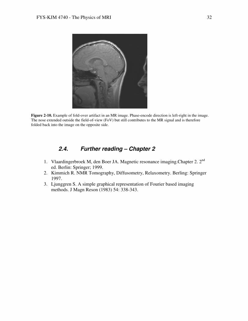
Note again that FoV here refers to the extent of the object which contributes to the measured MR-signal. Under sampling results in part of the object positioned outside the image FoV will be back-folded into the image, as shown in Figure 2-10. In the read-out (x) direction it is generally not a problem to avoid such back-folding since the sampling rate can be made very high on modern scanners. The ‘extra’ FoV containing the unwanted parts of the object can then simply be discarded in the reconstruction process as shown in Figure 2-8. However, in the phase-encode direction back-folding can be a problem since increasing the ‘sampling rate’ in the y-direction can only be achieved by increasing Ny (at the cost of scan-time) or by increasing FoVy (at the cost of resolution) so that the entire object is covered by the image FoV. Note that fold-over can also occur in the slice-direction in 3-D acquisitions since this direction is also phased encoded.
Back-folding in the phase-encoding directions can sometimes be reduced by careful selection of the phase-encoding direction relative to the dimensions of the object to be scanned.

FYS-KJM 4740 - The Physics of MRI 31
Figure 2-7. ‘Fold-over’ artifact in the phase encode direction if the objects extends beyond the field of view. The parts of the object outside the FoV are folded back into the image at the opposite end. Fold-over artifacts can often be eliminated by careful planning of the optimal phase-encode direction, by increasing Ny or by increasing the FoV.
Figure 2-8. Back-folding can be avoided by increasing the sampling rate and FoV. The resolution is preserved since Nx is also increased. The unwanted parts of the object FoV are discarded during
reconstruction.
Object
Image
FYS-KJM 4740 - The Physics of MRI 32
2.4. Further reading – Chapter 2
1. Vlaardingerbroek M, den Boer JA. Magnetic resonance imaging.Chapter 2. 2nd
ed. Berlin: Springer; 1999. 2. Kimmich R. NMR Tomography, Diffusometry, Relaxometry. Berling: Springer
1997. 3. Ljunggren S. A simple graphical representation of Fourier based imaging
methods. J Magn Reson (1983) 54: 338-343.
Figure 2-10. Example of fold-over artifact in an MR image. Phase-encode direction is left-right in the image. The nose extended outside the field-of-view (FoV) but still contributes to the MR signal and is therefore folded back into the image on the opposite side.

FYS-KJM 4740 - The Physics of MRI 33
3. Pulse sequences – an introduction We have seen that in order to reconstruct the spin density of the object we need to evenly sample the k-space representation of the object. Then the next question is; how do we know how to apply the gradients in the x- and y-directions in order to properly sample k-space and obtain an image? The short answer to this is that the required spatial resolution and coverage (i.e. size of object to be imaged) impose well defined constraints on the distance between consecutive samples, gradient strengths and duration as well as
the number of sample points (matrix size) in k-space. The relationship between k-space values and image resolution and field of view was discussed in the previous chapter. The challenge is now to apply the gradients in such a way that k-space is properly sampled and the process of applying gradients and RF-pulses in a certain sequence at certain intervals in order to obtain a proper sampling of k-space (and with a required sensitivity to differences in relaxation times) is referred to as a ‘pulse sequence’. Figure 3-1 shows the sequence diagram for a combination of gradients which enables sampling of a single point in k-space. In order to cover the entire k-space with this sequence it would have to be repeated Nx x Ny times (for a Nx x Ny imaging matrix). Although this would work, it is not a very efficient approach to sampling k-space because it requires the application of Nx x Ny RF-pulses with a given time-interval between each pulse (dictated by hardware constraints and required image contrast as discussed later). This is time consuming and would result in a very long acquisition time. The acquisition time can be reduced
kx
ky
RF
Gz
Gy
Gx
1 sample
kx
kyky
RF
Gz
Gy
Gx
RF
Gz
Gy
Gx
1 sample
Figure 3-1. A simplified pulse sequence to obtain a single sample point in k-space. The sequence
must be repeated Nx x Ny times to cover k-space with a matrix resolution of Nx x Ny datapoints.

FYS-KJM 4740 - The Physics of MRI 34
considerably by sampling multiple k-space points for each applied RF-pulse and this is the approach used in all practical pulse-sequences used today.
3.1. The Gradient Echo (GRE) sequence
Figure 3-2 shows a modified pulse sequence where one entire line of k-space is collected for each RF-pulse. This is achieved by applying a constant negative gradient in the x-direction during the application of the y-gradient. The negative Gx gradient moves
k(t) in the negative direction along the kx-axis. If the Gy gradient is also made to be negative at the same time, then k(t) moves downwards in the third quadrant of k-space as shown in Figure 3-2. If the polarity of the Gx gradient in now changed (and Gy is turned off) k(t) moves in a straight line parallel to the kx axis towards to fourth quadrant. During this time-interval the resulting MR signal is sampled along the discrete points shown in Figure 3-2. The Gx- and Gy- gradients are commonly referred to as the ‘read-out’ or ‘frequency encoding’ gradient and ‘phase encoding’ or ‘preparation’ gradient, respectively for Gx - and Gy. This is because Gy is used to introduce a controlled phase shift (unique for each line in k-space) whereas Gx is applied during the read-out of the signal and therefore introduces a position-dependent frequency modulation of the signal along the direction of the applied Gx-gradient.
RF
Gz
Gx
Gy
N samples
tskx
ky
= sample points
12
3 4
RF
Gz
Gx
Gy
N samples
tskx
ky
= sample points
RF
Gz
Gx
Gy
N samples
RF
Gz
Gx
Gy
N samples
tskx
ky
= sample points
12
3 4
Figure 3-2. The basic gradient echo sequence (left diagram) and the corresponding discrete sampling of one line
in k-space.

FYS-KJM 4740 - The Physics of MRI 35
Other methods exist whereby k-space can be sampled even more efficiently by
sampling multiple ky lines (as well as kx lines) for each RF-excitation. Echo-planar
imaging and fast spin echo are examples of such sequences and will be discussed in Chapter 6. The method outlined above whereby a single line along kx is sampled following each RF-pulse is still a widely used approach today and forms the basis for the two main classes of pulse sequences, namely gradient echo (GRE) and spin echo (SE) (see next section) sequences. Note that the RF-excitation for this type of sequence needs to be applied Ny times, where Ny equals the number of rows in k-space (i.e. the matrix resolution in the ‘y’-direction of the image. It is important to note that it is the resolution in the y-direction (i.e. the phase encoding direction) that is expensive in terms of imaging time since the shortest time-interval between successive RF-pulses is restricted by many factors as will be discussed later. The resolution in the read-out direction on the other hand does not significantly influence the total scan-time (but is also limited by hardware
RF
Gz
Gx
Gy
TE
Nx, samples, fs=1/ts
Gx_r
Gx_rew
Gy_max
Ty Tread/2
Repated Ny times
RF
Gz
Gx
Gy
TE
Nx, samples, fs=1/ts
Gx_r
Gx_rew
Gy_max
Ty Tread/2
Repated Ny times
Figure 3-3. The basic GRE sequence. For a Nx x Ny image matrix, the sequence must be repeated Ny times with Nx datapoints read out for each kx-line.
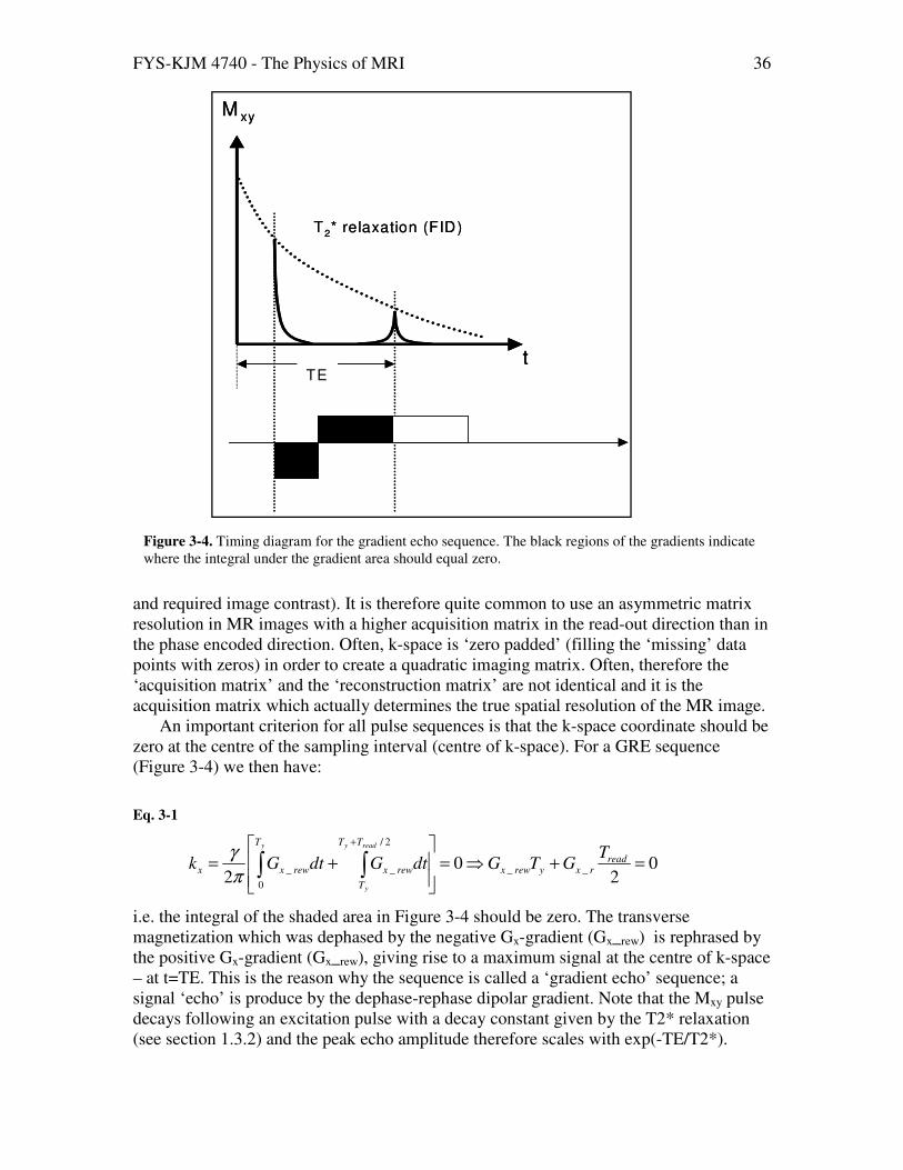
FYS-KJM 4740 - The Physics of MRI 36
and required image contrast). It is therefore quite common to use an asymmetric matrix resolution in MR images with a higher acquisition matrix in the read-out direction than in the phase encoded direction. Often, k-space is ‘zero padded’ (filling the ‘missing’ data points with zeros) in order to create a quadratic imaging matrix. Often, therefore the ‘acquisition matrix’ and the ‘reconstruction matrix’ are not identical and it is the acquisition matrix which actually determines the true spatial resolution of the MR image.
An important criterion for all pulse sequences is that the k-space coordinate should be zero at the centre of the sampling interval (centre of k-space). For a GRE sequence (Figure 3-4) we then have:
Eq. 3-1
02
02
__
2/
_
0
_ =+⇒=
+= ∫∫
+
readrxyrewx
TT
T
rewx
T
rewxx
TGTGdtGdtGk
ready
y
y
π
γ
i.e. the integral of the shaded area in Figure 3-4 should be zero. The transverse magnetization which was dephased by the negative Gx-gradient (Gx_rew) is rephrased by the positive Gx-gradient (Gx_rew), giving rise to a maximum signal at the centre of k-space – at t=TE. This is the reason why the sequence is called a ‘gradient echo’ sequence; a signal ‘echo’ is produce by the dephase-rephase dipolar gradient. Note that the Mxy pulse decays following an excitation pulse with a decay constant given by the T2* relaxation (see section 1.3.2) and the peak echo amplitude therefore scales with exp(-TE/T2*).
Figure 3-4. Timing diagram for the gradient echo sequence. The black regions of the gradients indicate where the integral under the gradient area should equal zero.
T2* relaxation (FID)
M xy
tTE
T2* relaxation (FID)
M xy
tTE

FYS-KJM 4740 - The Physics of MRI 37
Since image contrast is mainly determined by the information in the central part of k-space (see Figure 2-3) the time at which the echo is generated (called the echo time, TE) is of great importance for the contrast in the final image. This will be discussed in more detail in the next chapter.
3.2. The Spin Echo (SE) sequence
In the spin echo (SE) sequence the signal echo is generated by a second RF-pulse
rather than by switching the polarity of the read-out gradient. This approach has many advantages in terms of the achievable contrast in the resulting image, as discussed in the next chapter. In a SE sequence a 90o RF-pulse is followed by a 180o pulse. The purpose
Figure 3-5. The spin echo (SE) sequence. The k-space trajectory is shown for the readout of one k-space line.
RF
Gz
Gx
Gy
Nx samples
kx
ky
= sample points
12
3 4
t=0 t=TE/2 t=TE
Repeated Ny times
t=0
t=TE/2
t=TE
Ty
Tread
RF
Gz
Gx
Gy
Nx samples
kx
ky
= sample points
12
3 4
t=0 t=TE/2 t=TE
Repeated Ny times
t=0
t=TE/2
t=TE
Ty
Tread

FYS-KJM 4740 - The Physics of MRI 38
of the 180o RF pulse is the same as switching the polarity of the Gx gradient in GRE sequences; namely to move the k-vector to negative values and thereby allowing a complete kx-line to be sampled in each TR-interval where TR is the time interval between each 90o RF-pulse.
Figure 3-5 shows sequence diagram for the spin echo sequence. Note that the effect of the 180o is to invert the position in k-space (from 1st to 4th quadrant) thereby enabling read-out of one kx-line when applying a constant Gx gradient. Note also that the polarity of the Gx gradient is the same on both sides of the 180o pulse since a 180o pulse inverts the phase. Just like for the GRE sequence we require the net readout phase to be zero in the centre of k-space in order to generate a spin echo here. The total phase in the SE sequence is given by (see Vlaardingerbroek and den Boer p 67-68):
Eq. 3-2
θTE=-γ ( zGztdt+ yGy,ntdt+ xGxtdtTE20
TE20
TE20 2 +γ 3 zGztdt+ xGxtdtTE
TE2 TETE2 4
where each integral describe the area under the gradient-vs-time curve (Figure
3-5). Note that the z-gradient terms disappear (see Figure 3-6). The y- and x-components can now be expressed in terms of the k-space variables as for the GRE sequence:
Eq. 3-3
ynyny TGk ⋅= ,, γ and 'tGk xx ⋅= γ
where t’=(TE-t) so that kx=0 at t=TE.
Figure 3-6. The use of rewinder gradients to reverse the phase build-up introduced by the slice select gradient. Note that the 180 deg pulse inverts the phase (θz) whereas the 90 deg pulse nulls the phase at the time of the pulse peaks because the z-component of the signal is zero after the 90 deg pulse..
RF
Gz
θz
90o
180o

FYS-KJM 4740 - The Physics of MRI 39
4. MR signal behaviour and image contrast
So far we have focused on how to make an MR image using two main classes of pulse sequences, namely spin echo (SE) and gradient echo (GRE) sequences. We have up until now limited the discussion on signal behaviour to state the detectable transverse magnetization is proportional to the spin density distribution in the object to be imaged. We have also stated that the spin density is not a very sensitive contrast parameter in MRI (with some exceptions) since the water contents of different soft tissues is fairly constant. The real strength of MRI lies in it’s ability to visualize differences in proton relaxation values (T1, T2, T2*) between different tissues. Many pathologies cause alterations in the relaxation values and by making the pulse sequences sensitive to local variations in the relaxation times we can obtain MR images which are clinically useful. Since the contrast behaviour of SE and GRE sequences are quite different they will be discussed separately.
4.1. Spin Echo signal behaviour
What is then actually the point of generating a spin echo rather than a gradient echo?
We heard in Chapter 3.1 that it takes time to generate RF-pulses (especially 180o pulses), so there’s clearly no time-saving reason for this approach. The main purpose of the SE sequence has to do with the achievable contrast in this type of sequence versus in a GRE sequence. Figure 4-1 shows the rephrasing effect of the 180o pulse in a SE sequence.
T2* (FID)
M xy
TE
RF
T2 relaxation
T2* (FID)
M xy
TE
RF
T2 relaxation
T2* (FID)
M xy
TE
RF
T2 relaxation
Figure 4-1. The spin echo sequence generates echoes with amplitudes modulated by T2-relaxation times in tissue since static dephasing effects (T2* relaxation) are
eliminated by the 180o pulse.

FYS-KJM 4740 - The Physics of MRI 40
We discussed briefly in Section 1.3.2 that the signal (Mxy) decays exponentially with a decays constant T2* and that T2* generally is much shorter than the tissue-specific relaxation time T2 due to local inhomogeneities in the B0 field. The 180o RF-pulse (applied at t=TE/2) effectively rephrases the intra-voxel phase dispersions caused by the inhomogeneity term in T2* (Figure 4-2). Consequently, en echo (spin echo) is generated at t=TE. Whereas the gradient echo is unable to refocus field inhomogeneities RF-refocusing will effectively eliminate static field inhomogeneities. Note that only static
inhomogeneities are eliminated in the SE sequence; and relaxation due to diffusion in an inhomogeneous field (at the time-scale of TE) is not recovered in the SE sequence (nor in the GRE sequence).
The effect of RF-excitation pulses on the longitudinal (Mz) and transversal (Mxy) magnetization was discussed in Chapter 1.3.3 (Eq. 1-18 and Eq. 1-19) . Here we introduced the term ‘steady state’ describing the situation where the various magnetization components are constant prior to each new RF-pulse. Figure 1-7 depicted the approach to a steady-state situation after multiple RF-excitations. Let us first examine the influence of T1-relaxation on the z-magnetization following multiple RF excitation pulses. If we for now assume that a 90o flip angle is used (so that the z-magnetization just after the nth RF pulse Mz(t
+n)=0) Eq. 1-18 can be simplified to obtain the z-magnetization
Spin EchoSignal
90 pulseo
180pulse
oDephasing
Rephasing
RF
90o pulse
180o pulse
Spin echo
Gx
dephase rephase
Spin EchoSignal
90 pulseo
180pulse
oDephasing
Rephasing
RF
90o pulse
180o pulse
Spin echo
Gx
dephase rephase
Figure 4-2. The refocusing effect of the 180 deg pulse in a SE sequence.

FYS-KJM 4740 - The Physics of MRI 41
in the (n+1)th TR-interval (remember TR is the time interval between successive excitation pulses):
Eq. 4-1
56789 = 5: − ;5: − 5687< exp =− 7899 > = 5: ?1 − AB =− 7899 >C
This expression is valid only if we assume that the transverse magnetization has decayed to zero (or removed by other means) in the TR-interval. In SE sequences this means that
we need to have T2<<TR and in GRE sequences T2*<<TR. This requirement is typically met in SE sequences (but not in GRE sequences) since TR is typically between 300 and 2000 ms (and T2 < 150 ms in vivo for most tissues) in SE sequences.
Figure 4-3 shows the evolution of the Mz magnetization component in a SE
sequence. Note that, since 90o excitation pulses are used, a steady-state condition is established immediately after the first excitation pulse; i.e. Mz(t
-n+1)= Mz(t
-n) where
t
t=0
M0
Mz
90o pulses
0
T1=300 msT1=1000 ms
’contrast’
t
t=0
M0
Mz
90o pulses
0
T1=300 msT1=1000 ms
’contrast’
TR
Figure 4-3. The evolution of the Mz magnetization component following multiple 90o pulses for two different T1-values. Note that in the case of 90 o excitation, steady state condition is established already after the first RF-pulse.

FYS-KJM 4740 - The Physics of MRI 42
Mz(t-n) is the z-magnetizaton just prior to the nth RF pulse. For a given repetition time,
t=TR, Eq. 4-1 then becomes:
Eq. 4-2
[ ])/exp(1)( 10 TTRMTRM z −−=
If the spin echo is generated at t=TE the peak of the measured echo signal (proportional to the Mxy magnetization) is then given by (α=90o):
Eq. 4-3
[ ] )2/exp()1/exp(1)2/exp()sin()(),( 0 TTETTRMTTETRMTETRSI z −−−=−∝ α
which is the well known SE signal equation. The signal intensity (in arbitrary units) as a function of TR is shown in Figure 4-4 for three different sample tissues. The simulation was made with a short TE value of 15 ms (TE << T2) so that T2-relaxation can be ignored (exp(-TE/T2) ≈ 1). Optimal T1-contrast is achieved using a
0 500 1000 1500 2000 2500 3000 35000
10
20
30
40
50
60
70
80
TR (ms)
Rela
tive s
ign
al
T1/T2/rho = 1500 ms / 150 ms / 0.9
T1/T2/rho = 900 ms / 100 ms / 0.8
T1/T2/rho = 300 ms / 80 ms / 0.75
T1-weighted
rho-weighted
Figure 4-4. Signal as a function of TR in a SE sequence with short TE (15 ms) for three different tissues. T1-contrast is obtained by using a relatively short TR and the contrast becomes more
weighted towards proton density at longer (relative to T1) TR values.
FYS-KJM 4740 - The Physics of MRI 43
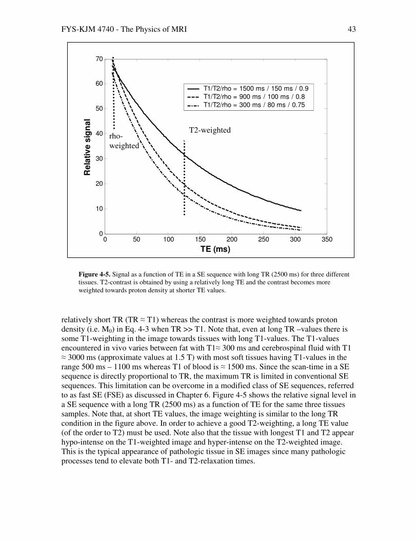
relatively short TR (TR ≈ T1) whereas the contrast is more weighted towards proton density (i.e. M0) in Eq. 4-3 when TR >> T1. Note that, even at long TR –values there is some T1-weighting in the image towards tissues with long T1-values. The T1-values encountered in vivo varies between fat with T1≈ 300 ms and cerebrospinal fluid with T1 ≈ 3000 ms (approximate values at 1.5 T) with most soft tissues having T1-values in the range 500 ms – 1100 ms whereas T1 of blood is ≈ 1500 ms. Since the scan-time in a SE sequence is directly proportional to TR, the maximum TR is limited in conventional SE sequences. This limitation can be overcome in a modified class of SE sequences, referred to as fast SE (FSE) as discussed in Chapter 6. Figure 4-5 shows the relative signal level in a SE sequence with a long TR (2500 ms) as a function of TE for the same three tissues samples. Note that, at short TE values, the image weighting is similar to the long TR condition in the figure above. In order to achieve a good T2-weighting, a long TE value (of the order to T2) must be used. Note also that the tissue with longest T1 and T2 appear hypo-intense on the T1-weighted image and hyper-intense on the T2-weighted image. This is the typical appearance of pathologic tissue in SE images since many pathologic processes tend to elevate both T1- and T2-relaxation times.
0 50 100 150 200 250 300 3500
10
20
30
40
50
60
70
TE (ms)
Re
lati
ve
sig
na
lT1/T2/rho = 1500 ms / 150 ms / 0.9
T1/T2/rho = 900 ms / 100 ms / 0.8
T1/T2/rho = 300 ms / 80 ms / 0.75
rho-
weighted
T2-weighted
Figure 4-5. Signal as a function of TE in a SE sequence with long TR (2500 ms) for three different tissues. T2-contrast is obtained by using a relatively long TE and the contrast becomes more
weighted towards proton density at shorter TE values.

FYS-KJM 4740 - The Physics of MRI 44
4.2. T1-weighted (Spoiled) Gradient Echo signal behaviour
We have mentioned in previous sections that the main advantage of GRE sequences
over SE sequences is the speed of acquisition. The increase in speed is achieved by the absence of an RF refocusing pulse which means that both TR and TE can be made substantially shorter than in a SE sequence. The signal behaviour in GRE sequences is generally much more complicated than in SE sequences for three main reasons:
1. A flip angle α <90o is commonly used (to maximize the signal at short TR) and
the MR signal therefore becomes a function of α. 2. The condition TR>> T2 can generally not be assumed which significantly
complicates the magnetization behaviour. 3. The MR signal depends on T1, T2 and T2* relaxation.
T1-w rho-w T2-wT1-w rho-w T2-w
Figure 4-6. Sample SE images in the brain. The sequence parameters were TR/TE = 500 ms / 20 ms (T1-w), 2200 ms / 20 ms (rho-w) and 2200 ms / 80 ms (T2-w)

FYS-KJM 4740 - The Physics of MRI 45
For the time being we assume that Mxy decays to zero within each TR-interval. This means that either we must have that TR >> T2 or the magnetization vector must actively be destroyed. This is commonly done in GRE sequences and is referred to as ‘spoiling’ or ‘spoiled’ GRE sequences. Mxy can be destroyed either by applying special ‘spolier’ gradients of by alternating the phase of the RF-excitation pulse. Note that TR must be >> T2 (not T2*). This is because two or more RF-pulses will always generate
spin echoes (and echoes with even more exotic names) if the interval between successive RF-pulses is sufficiently short compared to the T2-relaxation time. In this case, we have what is called ‘transverse coherence’ which will be discussed later in Chapter 5. With this assumption we can plot Mz as a function of time, following multiple RF-pulses using the same approach as for SE sequences (Section 4.1). As shown in Figure 4-7, the evolution of Mz now depends strongly on the flip angle used. With a flip angle of 90o steady state is established immediately (after the first RF-pulse), just like for the SE sequence, and the lower the flip angle the longer it takes to establish steady state condition. Figure 4-8 shown the evolution of the Mxy magnetization as a function of number of RF-pulses, using the same parameters as in Figure 4-7. We see that the steady state signal level is a function of flip angle and that the largest steady state signal is obtained for the lowest flip
0 200 400 600 800 1000 1200 14000
10
20
30
40
50
60
70
80
90
100
time
Mz (
a.u
.)
flip = 20 deg
flip = 50 deg
flip = 90 deg
Figure 4-7. The evolution of the longitudinal magnetization (Mz) following multiple RF-excitation pulses when TR << T1 (T1=600 ms , TR= 20 ms). Note that for flip angles < 90 deg the magnetization goes through a transient stage before a steady state level is reached. Notice also that the final magnetization level is flip angle dependent.
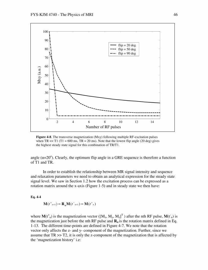
FYS-KJM 4740 - The Physics of MRI 46
angle (α=20o). Clearly, the optimum flip angle in a GRE sequence is therefore a function of T1 and TR.
In order to establish the relationship between MR signal intensity and sequence
and relaxation parameters we need to obtain an analytical expression for the steady state signal level. We saw in Section 1.2 how the excitation process can be expressed as a rotation matrix around the x-axis (Figure 1-5) and in steady state we then have:
Eq. 4-4
)()()( 11 nnn ttt+
+−
++ == MMRM
α
where M(t+
n) is the magnetization vector ([Mx, My, Mz]T ) after the nth RF pulse, M(t-
n) is the magnetization just before the nth RF pulse and Rα is the rotation matrix defined in Eq. 1-13. The different time-points are defined in Figure 4-7. We note that the rotation vector only affects the z- and y- component of the magnetization. Further, since we assume that TR >> T2, it is only the z-component of the magnetization that is affected by the ‘magnetization history’ i.e:
2 4 6 8 10 12 140
10
20
30
40
50
60
70
80
90
100
Number of RF pulses
Mx
y (
a.u.)
flip = 20 deg
flip = 50 deg
flip = 90 deg
2 4 6 8 10 12 140
10
20
30
40
50
60
70
80
90
100
Number of RF pulses
Mx
y (
a.u.)
flip = 20 deg
flip = 50 deg
flip = 90 deg
Figure 4-8. The transverse magnetization (Mxy) following multiple RF-excitation pulses when TR << T1 (T1 = 600 ms, TR = 20 ms). Note that the lowest flip angle (20 deg) gives
the highest steady state signal for this combination of TR/T1.

FYS-KJM 4740 - The Physics of MRI 47
Eq. 4-5
0)()( ','1',' == −+
−nyxnyx tMtM
01'11' )1()()( MEtMEtM nznz −+= ++
−
Eq. 4-6
−
−
−=
+
+
+
+
+
+
)(
)(
)cos()sin(
)sin()cos(
)(
)(
1'
1'
1'
1'
nz
ny
nz
ny
tM
tM
tM
tM
αα
αα
where E1=exp(-t/T1). Since My(t
-n+1)=0 this simplified to
Figure 4-9. The evolution of Mz (top) and Mxy (bottom) under steady state condition and for TR
>> T2 so that Mxy(t-n-1) = Mxy(t
-n+1)=0.
α α α
M z
n -1 n
M z( t -n )
M z( t+n)
M z(t -n + 1 )
n + 1
α
M z( t+n + 1 )
α α α
M z
n -1 n
M z( t -n )
M z( t+n)
M z(t -n + 1 )
n + 1
α
M z( t+n + 1 )
α α α
n -1 n n + 1
M xy
M xy(t -n ) M xy(t -
n + 1 )
M xy(t+n ) M xy(t+
n + 1 )
α α α
n -1 n n + 1
M xy
M xy(t -n ) M xy(t -
n + 1 )
M xy(t+n ) M xy(t+
n + 1 )

FYS-KJM 4740 - The Physics of MRI 48
Eq. 4-7
)()cos(
)sin(
)(
)(1'
1'
1'
+
+
+−
=
+
+nz
nz
nytM
tM
tM
α
α
Combining Eq. 4-5 and Eq. 4-7 we can then solve for My(t
+n) (=My):
Eq. 4-8
)cos(1
)1)(sin(
1
10'
α
α
E
EMM y
−
−=
This reduces to the signal equation for SE sequences (for α=90o). Note that Mx=0 so MT=My. The net transverse magnetization at the time of the gradient echo readout is modulated by T2* relaxation (Eq. 1-19) which gives:
Eq. 4-9
*)2/exp()cos()1/exp(1
))1/exp(1)(sin(),,( 0 TTE
TTR
TTRMTRTEM T −
−−
−−=
α
αα
This is the signal equation for a ‘spoiled’ gradient echo sequence. Since we assume
perfect spoling of the transverse magnetization (or TR >> T2) the signal is independent of T2-relaxation.
It is of interest to examine more closely the dependence of flip angle on MR signal in spoiled GRE sequences. Figure 4-11 shows the dependence of relative signal intensity (SI) on flip angle as a function of T1-relaxation time for a given TR. Note that the flip angle which gives maximum SI is a function of T1 (and TR). The ‘optimum’ flip angle (in terms of peak signal) is obtained by differentiating Eq. 4-9 with respect to flip angle:
Eq. 4-10
)1/exp()cos(0 TTRM
e
T −=⇒= αδα
δ
The flip angle αe is commonly referred to as the Ernst angle. We observe that αe descreases with decreasing T1 for a given TR and increases with decreasing TR for a given T1. The contrast weighting in a spoiled GRE sequence is either T1-weighted or T2*-weighted and the weighting depends on the TR/T1 ratio at given flip angle:
• Short TR (TR/T1 << 1) combined with large flip angle gives T1-weighting
• Long TR (TR/T1 ≈1) combined with low flip angle gives T2*-weighting

FYS-KJM 4740 - The Physics of MRI 49
Figure 4-10 shows spoiled GRE images of the brain with different combinations of TR / flip angle. Note that large α gives very little signal, especially at the shortest TR (top right image). This is because T1-values of brain parenchyma are about 700-1000 ms and a flip angle of 90o is therefore much larger than the Ernst angle for this TR-value. Note the bright appearance of blood in the same image. This is due to what is called ‘in-flow’ effects which gives rise to a short ‘apparent’ T1 of blood flowing into the imaged slice. Flow effects will be discussed in Chapter 10.
Rel SI
Flip angle90604020
T1=100ms
T1=300ms
T1=900ms
TR=50msRel SI
Flip angle90604020
T1=100ms
T1=300ms
T1=900ms
TR=50ms
TR=20 ms
α =60 α =90
TR=100 ms
α =20
TR=20 ms
α =60 α =90
TR=100 ms
α =20
Figure 4-11. Spoiled GRE image showing the effect of varying flip angle and TR on image contrast in the brain.
Optimal T1-weighting is achieved when using a short TR (relative to target T1) combined with a large flip angle.
Figure 4-10. Relative signal intensity versus flip angle in a spoiled GRE sequence for three different T1-relaxation times with TR = 50 ms.

FYS-KJM 4740 - The Physics of MRI 50
4.3. Multi-slice and 3D acquisitions
4.3.1. 2D multi-slice acquisitions
MRI is inherently a 3-dimensional technique since all excited spins within the object (covered by the transmit/receive coils) will collectively contribute to the measured signal. In the previous sections we discussed how one can selectively image a predefined slice through the object by using band-limited RF-pulses and slice-selective gradients. It is straight forward to acquire multiple 2D-slices in sequence by simply adjusting the
reference frequency of the RF-excitation pulse to equal to the Larmor frequency at the centre of the slice so that ωL=γ(B0 + Gzz) where z is the relative position along the slice-select gradient. Note that, if TR >> TE then multiple slices can be acquired per TR-interval as shown in Figure 4-12. Since the slice profile is not perfect, a certain amount of ‘cross-talk’ between slices will occur if adjacent slices are excited within a short time interval (relative to T1). This problem of ‘cross-talk’ can be overcome by either using interleaved slice ordering or by leaving a gap between consecutive slices. Note that the longer the TR-interval the more slices can be acquired per TR with no increase in scan time. If more slices are needed than what can be acquired within a TR-interval then two acquisitions must be made which will double the scan time.
The ‘free’ space within one TR-interval can also be used to acquire multiple echoes. This is very commonly done in SE sequences with a long TR. This way, both a
90
180
slice #1
slice #2
slice #3
slice #4
slice #1
TR
90
180
slice #1slice #1
slice #2slice #2
slice #3slice #3
slice #4slice #4
slice #1slice #1
TR
Figure 4-12. 2D multi-slice mode.

FYS-KJM 4740 - The Physics of MRI 51
proton weighted echo (short TE) and a T2-weighted echo (long TE) can be acquired in every TR-interval without any time penalty (Figure 4-13).
4.3.2. 3D acquisitions
The minimum achievable slice thickness in 2D-acquisitions is limited by the
available gradient strength, imperfections in the slice profile as well as signal-noise-ratio considerations (as will be discussed in Chapter 8). This limitation can partially be overcome by going to 3D-acquisition schemes. Here, the whole volume of interest is excited using non-selective RF-pulses and no slice selection gradient is applied. Instead, a second phase-encoding gradient is applied in the slice direction (Figure 4-14). The spin distribution is then given by the 3D Fourier transform of the magnetization vector:
Eq. 4-11
( )( )∫ ∫ ∫ ++=
x y zk k k
zyxzyxyxT dkdkdkzkykxkjkkMzyx exp),(2
1),,(
πρ
The slice thickness is then given by:
RF
Gz
Gx
Gy
t=0 t=TE1/2 t=TE1 t=TE2/2 t=TE2
RF
Gz
Gx
Gy
t=0 t=TE1/2 t=TE1 t=TE2/2 t=TE2
RF
Gz
Gx
Gy
t=0 t=TE1/2 t=TE1 t=TE2/2 t=TE2
Figure 4-13. Double echo SE sequence. The first echo is generally proton weighted and the second echo is T2-weighted.

FYS-KJM 4740 - The Physics of MRI 52
Eq. 4-12
zz TGz
max_
2
γ
πδ =
where Gz_max is the peak value of the phase encoding direction in the slice
direction and Tz is the gradient duration. The slice thickness is now only limited by the available gradient strength (and signal-noise considerations). Note that for 3D acquisitions, the scan-time is proportional to the number of slices since a new phase-encoding step must be applied in the z-direction for each new slice. This means that the scan-time for a 3D-acquisition is:
Eq. 4-13
NEXNNTRT zyacq ⋅⋅=
where NEX is the number of excitations; i.e. the number of times the whole sequence is repeated (to increase the overall signal-noise ratio). In spite of the increased acquisition time, 3D-acquisitions are commonly used today, especially in gradient echo sequences where TR can be made to be very short (< 5 ms), giving acceptable imaging times even for large isotropic (same resolution in all three dimensions) volumes. As an example, with TR=10 ms,128 slices and an acquisition matrix of 256 x 256, the entire volume can be acquired in just over 5 minutes. Note also that the signal-noise ratio in 3D acquisitions increases linearly with the number of slices acquired since each RF-pulse excites the entire volume. Comparison of a 3D-GRE and a 2D-SE acquisition is shown in Figure 4-15.
Figure 4-14. 2D (left) vs 3D GRE sequence. The slice-select gradient applied during RF excitation in 2D acquisitions is replaced by a second phase encode direction in the z-direction. In the 3D sequence the scan-time is proportional to the number of slices = number of phase encoding steps in the z-direction, Nz
RF
Gz
Gx
Gy
Slice selection
RF
Gz
Gx
Gy
Slice encoding
x Ny x Ny
x Nz

FYS-KJM 4740 - The Physics of MRI
Figure 4-15. 2D vs 3D acquisition. 3D acquisition is most commonly used in GRE sequences due to short TR – allowing e.g. whole-brain coverage with isotropic resolution with acceptable scansequences most commonly use 2D acquisitions because of long in the 2D sequence compared to the 3D sequence.
4.4. Further reading
1. Vlaardingerbroek M, den Boer JA. Springer; 1999
The Physics of MRI
2D vs 3D acquisition. 3D acquisition is most commonly used in GRE sequences due to short brain coverage with isotropic resolution with acceptable scan-time. Spin Echo
sequences most commonly use 2D acquisitions because of long TR times. Note the limited brain coverage in the 2D sequence compared to the 3D sequence.
Further reading – Chapter 4
Vlaardingerbroek M, den Boer JA. Magnetic resonance imaging. Chapter 2. Berlin:
53
2D vs 3D acquisition. 3D acquisition is most commonly used in GRE sequences due to short time. Spin Echo
Note the limited brain coverage
Magnetic resonance imaging. Chapter 2. Berlin:

FYS-KJM 4740 - The Physics of MRI 54
5. Steady state sequences
So far the discussion has been limited to signal behaviour in GRE sequences were either TR >> T2 or the transverse magnetization component has been actively destroyed prior to each RF-excitation. We shall now look into the signal behaviour for any steady state GRE sequence. Clearly, the situation now becomes more complicated since all components of the magnetization vector (Mx, Mx, Mz) in any given TR-interval are influenced by the magnetization history generated over previous TR-intervals.
5.1. Eight-ball echo
We have up until now made a clear distinction between SE and GRE sequences based on the assumption that in a SE sequence the echo is generated from two RF-pulses whereas in a GRE sequence the echo is generated from a single RF-pulse and a bipolar readout gradient. However, it is important to understand that any train of RF pulses (like in a GRE sequence) will, in general, generate multiple ‘spin echoes’. The echoes generated by multiple (two or more) RF-pulses are collectively referred to as ‘Hahn Echoes’ (the phenomenon was first described by E.L. Hahn in 1950). Imagine the effect of a train of equidistant 90o-pulses. The first pulse will flip the equilibrium magnetization
into the x’-y’-plane. If, at the time of the next pulse Mxy>0 (T2<TR) then one component of Mxy is flipped back along the z axis and one component remain in the x-y-plane. After a time t=2TR, the Mxy component will therefore partially refocus to form an echo. This is referred to as an ‘eight-ball’ echo. Note that this echo will be generated after two RF-pulses even in the case of full transversal dephasing (Mxy=0) in the TR-interval as shown in Figure 5-1. The first 90o pulse flips the magnetization around the y’-axis into the x’-y’-plane and Mxy is dephased by relaxation and the dephasing Gx gradient (A). Th3e second
90o Hahn echo
90o
Gx
x
y y
x
dephase rephase
z
y
x
TR TR
A B C
Figure 5-1. Generation of a Hahn echo (eight-ball echo) from two RF-pulses. The first pulse turns the z-component of the magnetization around the y-axis into the x-y-plane where it is dephased by the Gx gradient (A). The second pulse flips the transverse magnetization around the y-axis (B) resulting in a dephasing by Gx and consequent formation of a Hahn echo at time TR (C).

FYS-KJM 4740 - The Physics of MRI 55
90o pulse rotates each component of the transverse magnetization vector around the y’-axis into the y’-z’-plane (B). The y’-components of the magnetization resume their precession and an echo is formed when the phase angle acquired after the second 90o pulse equals the angle acquired before the pulse (C). If the magnetization distribution was displayed in 3 dimensions one would see that the magnetization vector traces a digit eight on the surface of a sphere (hence the name ‘eight-ball’), and that the transverse magnetization vector lie on a circle through the origin with the y’-axis as tangent. The curve that connects these points is called the ‘locus’. For the eight-ball echo, the sum vector of all the transverse magnetization components at the echo t=TE is 50% smaller than for the Spin Echo.
5.2. Stimulated echo
A second echo, called a stimulated echo, is formed after an additional RF-pulse, as illustrated in Figure 5-2. The second 90o-pulse flips the x’- component of the transverse magnetization back along the z-axis (A). This z-magnetization then carries with it the magnetization history from before the second 90o-pulse, but is not affected by the second dephasing gradient (B). The third pulse flips the z-magnetization back into the transverse plane along the x-axis (C). The third application of the Gx gradient now rephrases this transverse magnetization vector and a stimulated echo is formed (D). Note that, for every position in the object the transverse magnetization has a different magnitude and direction described by a locus in the transverse plane. This position – dependent magnetization behaviour in GRE sequences can cause severe artifacts if not corrected for.
Commonly, a flip angle less than 90o is used in GRE sequences, which will alter the shape of the echo loci, but does not otherwise alter the principles of echo formation discussed above. If we add the echoes generated by two- and three RF-pulses a total of five echoes are generated by three RF-pulses as shown in Figure 5-3. We can therefore conclude that a train of RF-pulses will generate a multitude of echoes, some of which are position dependent in magnitude and phase (affected by Gx) and some that are position independent. Following the notation of Vlaardingerbroek and den Boer we refer to the transverse component of the magnetization prior to an RF-pulse as the ECHO signal and the longitudinal component partially flipped into the transverse plane is referred to as an FID signal (Figure 5-4) We have previously introduced the term FID (free induction decay) to mean the ‘fresh’ longitudinal magnetization existing just prior to an excitation and partially flipped into the transverse plane by the pulse. This ‘fid’ (denoted by lower case letters) is only one component in the total FID (denoted by capital letters) since the latter also includes components flipped from the transverse plane back into the longitudinal plane by previous excitation pulses. Therefore, even though the ‘fid’ signal is position independent (in terms of influence by applied gradients) the FID signal is position depended, and so is the ECHO signal. Both the FID and the ECHO can be turned into a gradient echo in the usual way by a bipolar read-out gradient. In all cases, a gradient echo is formed when the time-integral between an excitation pulse and TE is zero.

FYS-KJM 4740 - The Physics of MRI 56
Figure 5-2. Formation of a stimulated echo from three 90o-pulses (along the y-axis). Note the variation in axis labels at the different stages. See text for details.
x
y
y
z
90o Stimulated echo 90o
Gx
x
y
z
y
x
z
y
90o
A
B
C D
α1 α2 α3
e1 e2 e3 e4 e5
Figure 5-3. Three excitation pulses yield five echoes. e1 is the eight-ball echo from α1 and α2; e2 is the stimulated echo of α1, α2 and α3; e3 is the refocused (by α3) e1; e4 is the eight-ball echo of α2 and α3 and
e5 is the eight-ball echo of α1 and α3.

FYS-KJM 4740 - The Physics of MRI 57
FID
Mxy
α α
ECHO
tn+1 tn
FID
Mxy
TE
α
echo
α
tn tn+1
ECHO Mxy
TE
α
echo
α
tn tn+1
Figure 5-4. Generation of gradient echoes from either the FID (left bottom) or from the ECHO (right
bottom) signals, according to the definitions of Vlaardingerbroek and den Boer.

FYS-KJM 4740 - The Physics of MRI 58
5.3. Steady state signal behaviour
We will now look at the signal behaviour in the general case for GRE sequences
where both transverse and longitudinal magnetization is present prior to each RF-pulse in steady state. As we discussed in the previous section, we then have a situation where the signal at each excitation pulse is the sum of multiple signals (primary and stimulated echoes) from previous excitation pulses. Mathematically, the spin dynamics can be described in terms separate matrices for excitation, precession and relaxation. The rotation matrix around the x’-axis following excitation by a α-degree RF-pulse, Rα was defined in Chapter 1.2 and is given by:
Eq. 5-1
−
=
)cos()sin(0
)sin()cos(0
001
αα
ααx'α,R
We can similarly define precession in the x’-y’-plane by a rotation matrix around the z’-axis:
Eq. 5-2
−=
100
0)cos()sin(
0)sin()cos(
θθ
θθ
z'θ,P
As shown in Figure 5-6 the phase angle θ is position dependent since it depends on the strength of the field gradient at position r: θ(r,t)=- γ ∫G.rdt. The phase angle θ can also include a component due to phase cycling of the RF-pulse; i.e. the effect of altering the phase of the RF-pulse at successive excitations (e.g. as used in RF-spoiling; see Vlaardingerbroek and den Boer for details).
Relaxation was introduced in Chapter 1.3.3, and we can express the effects of relaxation on the magnetization components (Eq. 1-18 and Eq. 1-19) in matrix notation as:
Eq. 5-3
0MMM )1()(
00
00
00
)( 1
1
2
2
1 Et
E
E
E
t nn −+
= ++
−
where M = [Mx,My,Mz]
T , M0=[0,0,M0]T, E2 = exp(-t/T2) and E1=exp(-t/T1).

FYS-KJM 4740 - The Physics of MRI 59
Since relaxation and precession occur at the same time, we can combine Eq. 5-2 and Eq. 5-3(transversal component) which then gives:
Eq. 5-4
0MMM )1()(
00
0)cos()sin(
0)sin()cos(
)( 1
1
22
22
1 Et
E
EE
EE
t nn −+
−= ++
− θθ
θθ
or
Eq. 5-5
0MMQM )1()(),2,1()( 11 EtEEt nn −+= ++
− θ
The steady state magnetization just after the (n+1)th pulse can now be calculate by multiplication with the rotation matrix Rα:
Eq. 5-6
)()()( 11 nnn ttMt+
+−
++ == MRM
α
y’
x’
z’
MT(r2,t’)
MT(r1,t’)
My
Mz
-θ
θy’
x’
z’
MT(r2,t’)
MT(r1,t’)
My
Mz
-θ
θ
Figure 5-5. Precession of the transverse magnetization initially along the y’-axis depends on the local
gradient at position r. At time t’ a position-dependent phase dispersion is established.

FYS-KJM 4740 - The Physics of MRI 60
Combining Eq. 5-5 and Eq. 5-6 we get:
Eq. 5-7
0αMRMQRU )1()()( 1Et n −=− +
α
where U is the unit matrix. The magnetization vector can then be expressed as:
Eq. 5-8
0αMRQRUM )1()()( 1
1Et n −−= −+
α
This set of three coupled linear equations can be solved in terms of the total transverse magnetization; MT = Mx’ + jMy’ giving:
Eq. 5-9
),(),()cos(
))exp(1)(sin()1(),(),,( 0
210 θα
θ
θα ++ =+
−−−= FyxM
DC
jEEyxMtyxM nT
where M0(x,y) is the spin density in the excited slice and
Eq. 5-10
))cos(1)(1( 12 α+−= EEC 2
211 ))cos(())cos(1( EEED αα −−−=
From Eq. 5-9 the following can be concluded:
1. The equation reduces to the ‘spoiled’ GRE expression in Eq. 4-8 when E2=exp(-
t/T2)=0 (TR >> T2). In this case, the factor D in the denominator depends on T1-weighting (through E1) only.
2. The term 1-E2exp(-jθ) in the numerator implies a varying degree of T2-weighting, dependent on θ, and hence position (see Figure 5-6). This means that, if E2 >0 the image will contain ‘bands’ of varying degree of T1- and T2-weighting depending on the value of exp(-jθ(r)) at a given position .
Eq. 5-9 describes the transverse magnetization immediately after an excitation pulse (MT(t+
n)). During the time-interval between the nth and the n+1 th pulse the magnetization will decay due to T2 effects as well as applied gradients:
Eq. 5-11
)),(exp()2/exp(),,(),,( trjTttyxMtyxM nTT ϕ−= +

FYS-KJM 4740 - The Physics of MRI 61
where ∫=t
tn
dttrGtr ),(),( γϕ and tn < t < tn+1 so for t= tn+1, φ(r,t)=θ
As discusses in Chapter 3.1, the gradient echo is generated by applying a bipolar gradient in the read-out (x’-) direction and a stepwise phase encoding gradient in the y’-direction:
Eq. 5-12
∫ ∫ +−= +
x y
ynyx dxdyyTGxtGjFyxMTttS ))'(exp(),(),(*)2/exp()'( ,0 γθα
where t’ = t-tn and Ty is the duration of the phase-encode gradient and Gy,n is the value of Gy at the nth profile. This is the signal equation for the FID signal in Figure 5-4. Equation Eq. 5-12 is similar to Eq. 2-17, which describes the MR signal as the Fourier transform of
the spin density. Note that we have replaced T2 by T2* in Eq. 5-12 since the gradient echo does not recover relaxation due to static inhomogeneities (see Chapter 1.3.2). The spin density is proportional to M0(x,y)) but now we have included the effects of relaxation and the position dependent phase dispersion described by the F+ term in Eq. 5-12. By making this term independent of θ we can then recover the true distribution of spin densities equally weighted by relaxation effects across the object. This will be discussed further in the next section.
0 2 4 6 80
5
10
15
20
|Mxy|Mxy (spoiled)
Phase angle (rad)
Tra
nsv
erse
mag
neti
zat
ion
|M
xy
|
Figure 5-6. Transverse magnetization (Mxy) as function of phase angle θ according to Eq. 5-9 (T1=1000 ms , TR=30 ms and flip = 50 deg). Since θ is position dependent (through the applied gradients) the MR-signal is modulated by this periodic variation in Mxy , creating bands in the MR image with varying T1 and T2 weighting. The magnetization in a spoiled GRE sequence (dotted line) is
independent of θ since Mxy is removed (through spoiling) prior to each new RF-pulse

FYS-KJM 4740 - The Physics of MRI 62
We can now similarly derive the signal equation for the ECHO signal. The transverse magnetization just before an RF-pulse is then given by:
Eq. 5-13
),(exp()2/exp(),,(),,( 1 yxjTTRtyxMtyxM nTnT θ−= ++
−
Since E2=exp(-TR/T2) we then have that
Eq. 5-14
DC
EEjEyxMtyxM nT
+
−−=+
−
)cos(
)))(exp(1)(sin(),(),,( 221
01θ
θα
Referring to Figure 5-4 we observe that, in order to form a gradient echo at t’=TE out of the ECHO signal at t’=0, the net gradient surface between TE and the next pulse must be zero following a single gradient reversal. The measured signal is then:
Eq. 5-15
∫ ∫ += +
x y
ynyx dxdyyTGxtGjFyxMTTEtS ))'(exp(),(),()2/exp()'( ,0 γθα
Note the positive exponent exp(TE/T2) since TE here describes the ‘negative’ time between the RF-pulse and the generation of the gradient echo from the ECHO (occurring earlier in time). We assumed in Eq. 5-13 that the T2-relaxation took place in the entire TR-interval (through the exp(-TR/T2) term) but since we generate the echo prior to the full TR, we have multiply by the positive exponent exp(TE/T2). (Note that if TE=TR the two terms cancel and we are left with the expression for the FID signal). We see that the gradient echo off the ECHO signal can be regarded as a gradient echo off the FID signal played out in reverse. We see that the ECHO signal is also a complicated, periodic function of θ, giving rise to bands of varying T1- and T2- weighting unless corrected for. In the next section we shall discuss different ways of obtaining ‘useful’ steady state GRE images by eliminating the position dependent effect of θ.
5.4. Steady state GRE sequences
As discussed previously, the main reason why we want to use GRE sequences in
the first place is speed combined with reasonable image quality. On modern MR-systems GRE sequences can have TR < 10 ms allowing high resolution volumes to be acquired in a few minutes and single 2D-slices to be generated in a few seconds. We will limit the discussion here to GRE sequences where TR << T1 and < T2. When TR > T1 the usefulness of GRE sequences (in terms of speed relative to SE sequences) is limited and the signal behavior is well defined (see Chapter 4.2). As discussed in the previous section, the problem of using very short TR’s is the presence of transverse magnetization coherence, which causes the MR-signal to be a complex function of both T1- and T2-relaxation and which will also give rise to artifacts since the degree of T1- and T2-

FYS-KJM 4740 - The Physics of MRI 63
weighting is position dependent. In order for a GRE sequence to be useful in practice, these artifacts therefore need to be eliminated and the signal behavior must be well defined function of T1 or T2 (ideally just one or the other).
There are three main approaches which are used to achieve this (with reference to Eq. 5-9 and Eq. 5-14):
1. Make θ large (large net gradient surface) relative to the voxel size so
that the bands of varying T1- and T2-weighting is averaged out over each voxel.
2. Apply RF- or gradient spoiling; removing all transverse coherence prior to each RF-pulse.
3. Make θ = 0 by balancing all gradients at the time of the signal readout
GRE sequences are named according to which of the three above approaches are used; The problem is, however, that each MR vendor uses different names for their particular sequence implementation. In Vlaardingerbroek and den Boer a ‘generic’ naming system is introduced whereby gradient echo sequences are logically named according to which of the three categories above is used. In this text book, gradient echo sequences in general are referred to as FE (field echo) or FFE (fast field echo) sequences. Note that these acronyms are used on Philips scanners only and we have in this compendium therefore used the even more generic term gradient echo – GRE. Figure 5-7 defines the different GRE sequences according to the division explained above (items 1-
GRE
θ=0
(method 3)
B-GRE (trueFISP,
balanced FFE)
spoiling
(method 2)
T1-GRE
θ=large
(method 1)
FID: N-GRE
(FAST, GRASS, FISP)
ECHO: T2-GRE (SSFP, PSIF, CE-
FAST)
Figure 5-7. Steady state GRE sequences grouped according to method, as defined in Vlaardingerbroek and den Boer. The names in brackets are commonly used acronyms used by different MR machine
vendors.

FYS-KJM 4740 - The Physics of MRI 64
3). This figure is adapted from Figure 4.17 in Vlaardingerbroek and den Boer. We shall now discuss each of these methods in more detail.
5.4.1. Large net-gradient surface
In this approach we make θ large relative to the pixel size so that the bands of
varying T1- and T2-weighting is averaged out over the pixel dimension. This approach can be used when reading out either the ECHO signal or the FID signal. The idea is to make the signal in each voxel the average of the signal from all isochromats3. The phase due to e.g. a gradient applied in the x-direction is given by:
Eq. 5-16
∫ == uxx txGdttGx γγθ )(
where tu is the time of the uncompensated gradient duration; i.e. from the time of the centre of the gradient echo to the time when the read-out gradient is switched off prior to next excitation pulse. From this we can see that the periodicity of F+(θ) (in Eq. 5-9) is
given by the wavelength: uxtGγ
πλ
2= and the pixel dimension is given by (see Chapter
3.1) : acqxtG
xγ
πδ
2= so that λ/δx=tacq / tu. This means that the periodicity of F+(θ) is
averaged out within one voxel when the uncompensated gradient surface is larger than the gradient surface during acquisition. This averaging can be expressed analytically (for FID gradient echo) by integrating Eq. 5-9 over θ from –π to π:
Eq. 5-17
∫−
+
−−=
π
π
θθ
θα
πd
DC
jEEyxMyxMT
)cos(
))exp(1)(1)(sin(),(
2
1),( 210
It can be shown that the solution to this integral is given by:
Eq. 5-18
−
−
+−=+
222
210
)sin()1(),(),( E
CD
DEC
C
EyxMyxM T
α
3 An isochromat is defined as a sub-set of spins within a voxel which experience the same gradients in all
dimensions so that they collectively can be described by a single magnetization vector with a given phase θ.

FYS-KJM 4740 - The Physics of MRI 65
This is the analytical expression for the relative signal strength in N-GRE sequence. It can similarly be shown that the signal in T2-GRE sequences (using the expression for the ECHO signal,Eq. 5-14 and Eq. 5-17) is given by:
Eq. 5-19
−
+−
−=−
22
2210 1
)sin()1(),(),(
CD
CED
C
EEyxMyxM T
α
5.4.2. Balanced GRE – TrueFISP
In B-GRE sequences, all gradients are completely compensated for (in Eq. 5-9) so
that θ=0 at the end of each TR-interval. This means that a single refocused magnetization vector is present in the transverse plane at each RF-excitation and no ‘splitting’ of the transverse magnetization occurs. This sequence, commonly referred to as TrueFISP, has become extremely popular over the last years due to the very interesting properties, as discussed below. It can be shown that the steady state transverse magnetization in a B-GRE sequence is given by:
Eq. 5-20
2121
21
0)cos()(1
)1)(sin(
EEEE
EEMM T
−−−
−=
α
α
Unlike all other GRE sequences balance GRE can be made virtually insensitive to
T2* effects. It can be shown that the effects of field inhomogeneities are refocused at TE=TR/2, leaving only T2-attenuation (like in SE sequences). This T2-attenuation is included in the above expression thought the √E2 term which is equal to exp(-TE/T2) for TE=TR/2.
For very short TR’s (TR << T1,T2) and large flip angles (α> αe) it can be shown that the relative signal in the B-GRE sequence is given by:
Eq. 5-21
1
2
)cos(1
)sin(
)2/1))(cos(1()cos(1
)sin(0
T
T
TTMM T
α
α
αα
α
−≈
−++=
i.e the signal is proportional to the ratio of T2/T1 and independent of TR. The optimal flip angle (maximum signal) is then:

FYS-KJM 4740 - The Physics of MRI 66
Eq. 5-22
21
21)cos(
TT
TTe
+
−=α
which results in the peak signal amplitude:
Eq. 5-23
1/22
10, TTMM peakT =
The peak magnetization, and hence signal to noise ratio (SNR), in a balanced GRE sequence is potentially extremely high. In fact – in pure water (T2≈T1) – almost 50% of the total equilibrium magnetization (that is, up to 50% of the total available spin polarization) is contributing to the signal! The B-GRE sequence therefore offers potentially much higher SNR ratio than any other steady-state GRE sequences, as seen in Figure 5-9. Note that we have so far ignored the influence of field inhomogeneities (δB0) on θ. When the gradient moment in all directions is truly zero at the time of signal readout, then θ is still likely to differ from zero due to the δB0 component (which is not compensated for by the zero net gradient surface). This gives rise to the same types of banding artefacts as discussed in the previous chapter but this time generated by δB0 rather than G(t). There are several approaches available to compensate for this, as discussed in Vlaardingerbroek and den Boer. The simplest and most obvious approach is to make TR very short (< 5 ms) so that errors due to δB0 not have time to develop. The fact that we are dealing with a single large refocused vector in the B-GRE sequence can give rise to large oscillations in the magnetization vector in the transient state. As an example, assume that a flip angle of 90o is used. The first RF-pulse will flip M0 into the transverse plane and (assuming TR << T1,T2) the next RF-pulse will flip almost the entire M0 back along the +/- z-axis (depending on the phase of the RF-pulse).
Therefore, after the second pulse there will be no magnetization left in the transverse plane and therefore no signal is generated. The third pulse will give a large signal and the fourth pulse no signal and so on. Due to T1- and T2- relaxation a steady state situation will eventually be established but this may require a large number of RF-excitations and the oscillatory transient state may be prohibitively long. The problem can be overcome by a simple trick. If the first RF-pulse has a flip angle of α/2 and the remaining pulses have alternating flip angles of +/- α then no oscillations will occur and the signal will approach steady state in a smooth fashion with a rate determined by T2-relaxation. The scheme is shown in Figure 5-7. Figure 5-10 shows the transient magnetization response with (right) and without (left) the initial π/2 pulse. Note the severe oscillations when the π/2 pulse is not applied. The simulation was done with TR/T1/T2/α = 5 ms / 900 ms / 100 ms/ 50o.

FYS-KJM 4740 - The Physics of MRI 67
x’
z
α/2
x’
z
-α
z
+α
x’
x’
z
α/2
x’
z
-α
z
+α
x’
Figure 5-8. The use of an initial π/2 pulse followed by +/- π/2 pulses in TrueFISP sequences avoids oscillation
of the transverse magnetization component in the transient state.
0 25 50 75 1000
5
10
15
20
B-GREN-GRET2-GRET1-GRE
flip angle (deg)
Rel
sig
nal
Figure 5-9. Rel signal (% of Mo) (T1/T2 = 900ms/100ms, TR/TE=5 ms / 2.5 ms) as function of flip angle for the four different classes of GRE sequences. Note the very large peak signal
for the B-GRE (trueFISP) sequences in spite of the very short TR.

FYS-KJM 4740 - The Physics of MRI 68
5.4.3. T1-GRE – Spoiled GRE
This class of GRE sequences was discussed previously (Chapter 4.2) where the
signal equation for this sequence was derived using a different approach. Spoiling of the transverse coherence prior to each RF-excitation is equivalent to setting E2=0 (and M(x,y,t-)=0 ) in Eq. 5-9 and Eq. 5-14. This results in a smooth approach to steady state, as shown in Figure 5-13. From Eq. 5-14 we then get:
Eq. 5-24
*)2/exp()cos(1
)1)(sin(),(),(
1
10 TTE
E
EyxMyxM
T−
−
−=
α
α
which is the same as Eq. 4-9. When TR << T1 we can make the approximation that 1-E1=TR/T1. If we also have that TE << T2* and α >> αe (the Ernst angle, defined in Eq. 4-10) then the signal in a spoiled GRE sequence is purely T1-weighted and is given by:
Eq. 5-25
1)cos(1
)sin(),(),( 0
T
TRyxMyxM T
α
α
−=
i.e. the signal is proportional to 1/T1, which is a very interesting feature in many applications as will be discussed in more detail in later chapters. Note that whereas in the
0 50 100 150 200 2500
0.2
0.4
0.6
0.8
No of RF-pulses
Tra
nsv
erse
mag
net
izat
ion
0 50 100 150 200 2500.1
0.2
0.3
0.4
0.5
No of RF-pulses
Figure 5-10. The approach to steady state in a TrueFISP sequence without (left) and with (right) an initial α/2 pulse as shown in Figure 5 8. Note the almost complete absence of oscillations when the α/2 pulse is used giving
a smooth approach to steady state. The steady state signal, as given by Eq. 5-20 is shown as dotted lines.
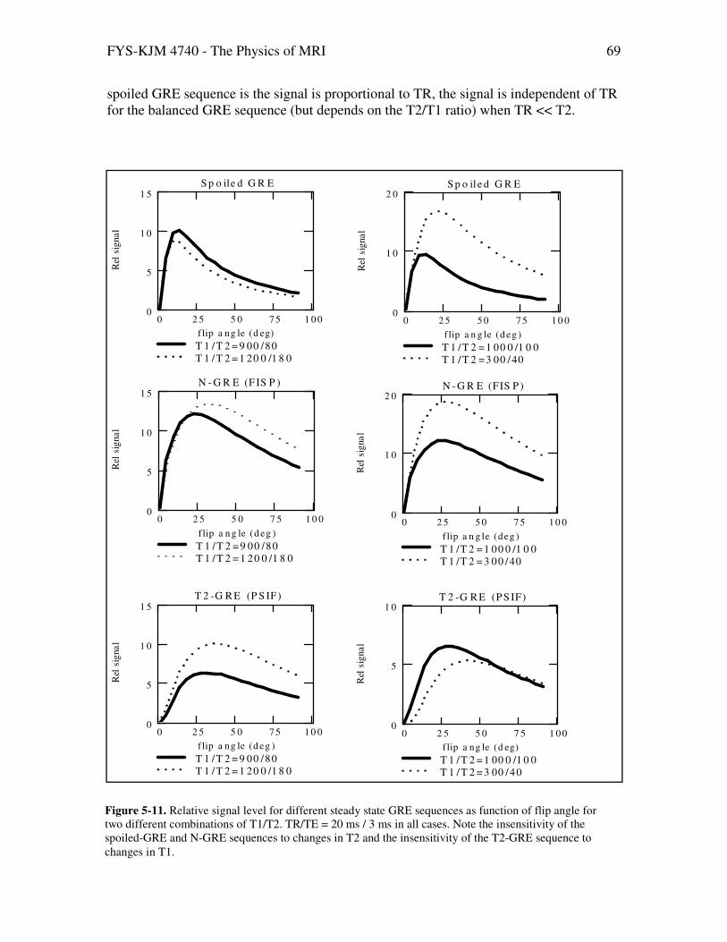
FYS-KJM 4740 - The Physics of MRI 69
spoiled GRE sequence is the signal is proportional to TR, the signal is independent of TR for the balanced GRE sequence (but depends on the T2/T1 ratio) when TR << T2.
0 2 5 5 0 7 5 1 0 00
1 0
2 0
T 1 /T 2 = 1 00 0 /1 0 0T 1 /T 2 = 3 00 /40
S p o il e d G R E
f lip a n g le (d eg )
Rel
sig
na
l
0 2 5 5 0 7 5 1 0 00
5
1 0
1 5
T 1 /T 2 = 9 00 /80T 1 /T 2 = 1 20 0 /1 8 0
N - G R E (F IS P )
f lip a n g le (d eg )
Rel
sig
na
l
0 2 5 5 0 7 5 1 0 00
5
1 0
1 5
T 1 /T 2 = 9 00 /80T 1 /T 2 = 1 20 0 /1 8 0
T 2 -G R E (P S IF)
f lip a ng le (d eg )
Rel
sig
na
l
0 2 5 5 0 7 5 1 0 00
1 0
2 0
T 1 /T 2 = 1 00 0 /1 0 0T 1 /T 2 = 3 00 /40
N - G R E (FIS P )
f lip a n g le (deg )
Rel
sig
na
l
0 2 5 5 0 7 5 1 0 00
5
1 0
1 5
T 1 /T 2 = 9 00 /80T 1 /T 2 = 1 20 0 /1 8 0
S p o ile d G R E
f lip a ng le (d eg)
Rel
sig
na
l
0 2 5 5 0 7 5 1 0 00
5
1 0
T 1 /T 2 = 1 00 0 /1 0 0T 1 /T 2 = 3 00 /40
T 2 -G R E (P S IF)
f lip a ng le (d eg)
Rel
sig
na
l
Figure 5-11. Relative signal level for different steady state GRE sequences as function of flip angle for two different combinations of T1/T2. TR/TE = 20 ms / 3 ms in all cases. Note the insensitivity of the spoiled-GRE and N-GRE sequences to changes in T2 and the insensitivity of the T2-GRE sequence to
changes in T1.

FYS-KJM 4740 - The Physics of MRI 70
5.1. Transient signal response
So far we have assumed that the signal has reached its steady state level before any data is acquired. The approach to steady state can, however, be a slow process which consequently requires the application of many ‘dummy pulses’ before the sequence is initiated. The situation is depicted in Figure 5-13 for a spoiled GRE and a N-GRE sequence, respectively in a tissue with T1/T2=900 ms / 100 ms using TR/flip = 10 ms/50o. We see that the non-steady state phase is especially troublesome for the N-GRE sequence. The presence of remnant transverse magnetization prior to each new RF-pulse in this sequence gives rise to severe oscillations and a slow approach to steady state. Acquisition of data during the transient phase therefore leads to modulation of the signal by the transient response. For the T1-GRE sequence the transient response causes mainly blurring (modulation by an exponential decay curve) whereas for the N-GRE the non-steady state oscillations cause both blurring and ghosting artifacts.
The severity of these oscillations can be reduced by gradually increase the flip angle to the final value, as shown in Figure 5-14.
Figure 5-12. Comparison of image contrast for (left->right) T1-GRE , N-GRE, T2-GRE and B-GRE (trueFISP).
TR/TE /flip = 20 ms / 3 ms / 20 deg for 1-3 and 4 ms / 2 ms / 70 deg for B-GRE.

FYS-KJM 4740 - The Physics of MRI 71
Figure 5-13. Simulation of the difference in transverse magnetization evolution between a spoiled (T1-GRE) and non-spoiled (N-GRE) sequence during the first 50 RF-pulses (TR/T1/T2/ flip = 10 ms / 900 ms /100 ms/ 50 deg). The T1-GRE sequence has rapid and smooth approach towards steady state,, whereas the N-GRE sequence
exhibits severe oscillations during the transient stage and a slower approach to steady state..
0 10 20 30 40 500
0.2
0.4
0.6
0.8
T1- GREN- GRE
No of RF-pulses
Tra
nsv
erse
mag
net
izat
ion
Figure 5-14. The transient oscillations in the N-GRE sequence can be reduced by initially using a lower flip angle which is gradually increased to the final value. In this example, the flip angle was increased from 20 deg to the final value of 80 deg for the first five excitations.
0 5 10 150
0.5
1
Increasing flip
Constant flip
# of RF pulses
Tra
nsv
erse
mag
net
izat
ion

FYS-KJM 4740 - The Physics of MRI 72
5.2. Further reading – Chapter 5
1. Vlaardingerbroek M, den Boer JA. Magnetic resonance imaging. Chapter 4.
Berlin: Springer; 1999 2. Scheffler K and Lehnhardt S. Principles and applications of balanced SSFP
techniques. Eur Radiol (2003) 13:2409-2418 3. Scheffler K. A pictorial decription of steady-states in rapid magnetic resonance
imaging. Concepts in Magnetic Resonance (1999) 11(5): 291-304. 4. Hahn EL. Spin Echoes. Phys Rev (1950) 80(4).

FYS-KJM 4740 - The Physics of MRI 73
6. Accelerated k-space trajectories
In all pulse sequences discussed so far, a single line of k-space is read out per TR-interval. This is the case both for SE and GRE sequences. The total scan-time per slice (or for the number of slices that can be acquired within one TR-interval, see Chapter 4.3.1) is therefore proportional to TR.Ny in 2D-mode and to TR.Ny
.Nz in 3D-mode (Nz = number of slices). The scan-time in conventional SE imaging is therefore long when strong T2-weighting (long TR,TE) is required and can in particular be prohibitively long in 3D-acqusitions. As an example, in a 3D-SE sequence with TR=2500 ms it would take more than 17 hours to acquire 100 slices with a matrix size of 256!
The acquisition time can be significantly reduced by acquiring multiple k-lines per TR-interval. We discussed briefly in Chapter 4.3.1 how multiple echoes could be acquired in one TR-interval if TE<<TR but here we assumed that the same phase-encoding was applied to both echoes resulting in two separate images with different echo time. If in stead a separate (and different) phase encoding is applied to individual echoes generated within a TR-interval then all echoes can be made to contribute to the same image. This is by no means a new idea; it was suggested by Peter Mansfield already in 1977 as a means of speeding up the acquisition of gradient echo images. He named this approach echo-planar imaging (EPI). The same technique was introduced for spin echo sequences in 1988 by Jörgen Henning under the name rapid acquisition with refocused
echoes (RARE ). The RARE technique it is today generally referred to as fast spin echo (FSE).

FYS-KJM 4740 - The Physics of MRI 74
6.1. Fast Spin Echo (FSE)
The fast spin echo (FSE) sequence and corresponding k-space trajectory is shown
in Figure 6-1. Comparing this to the conventional SE sequence (Figure 3-5) we see that, in stead of reading out a single ky-line per TR we now read out multiple lines per TR which are individually phase encoded. In theory, all ky-lines could be read out in a single TR. In this case, a single 90o pulse would be followed by Ny 180o pulses. This is called a ‘single shot’ sequence and requires very large system stability and homogeneity since the
RF
Gx
Gy
A B C D E F0
e1e2 en
G H
RF
Gx
Gy
A B C D E F0
e1e2 en
G H
ky
kx
0AB
C De1
EF
GHe2
ky
kx
0AB
C De1
EF
GHe2
Figure 6-1. The fast spin echo (FSE) sequence and corresponding k-space trajectory

FYS-KJM 4740 - The Physics of MRI 75
last echoes in the echo train will have a very low amplitudes due to the long echo time. We immediately observe the potential increase in acquisition speed of a FSE sequence relative to the SE sequence. If N echoes are generated in each TR-interval, the acquisition time is reduced by the same factor N. In practice, for multi-slice acquisitions, the time gain may not be as large as N, however since the generation of many echoes will leave less time to acquire multiple slices within the TR-time. Figure 6-2 defines some important parameters in a FSE sequence. The number of echoes acquired in each TR-interval is called the echo train length (ETL) (=1 for conventional SE and Ny for single shot FSE). ETL is also referred to as the ‘turbo factor’ since it determines the speed increase relative to a standard SE sequence (Tacq=TR.Ny/ETL). The time between consecutive echoes is called the echo spacing (ES). The effective echo time (TEeff) refers to the time between the 90o pulse and the formation of the echo closest to the centre of k-space (in the ky-direction). As seen from Figure 6-1, this is where the largest amplitude echo occurs since the phase encoding gradient is here at a minimum (or zero). We discussed in Chapter 2.2 that the image contrast is mainly determined from the information collected at the centre of k-space. Therefore, the echoes generated close to the k-space centre determine the effective echo time and hence image weighting. In Figure 6-2 the centre of k-space (no phase encoding) was placed at the centre of the echo train but we can in theory (but not in practice) place the centre point anywhere we like. Figure 6-3 shows two commonly used profile orders. The linear order already discussed gives a long TEeff. Alternatively, a so-called centric ordering can be used if TEeff should be as short as possible. In this case the lowest ky-line is acquired first in the echo train. One could also use a ‘mirrored’ centric ordering where the lowest ky-line is acquired at the very end of the echo train giving the longest possible TEeff.
The signal behaviour of the FSE sequence is in most respects very similar to the conventional SE sequence. The generation of multiple, individually phase encoded echoes does, however, introduce some important effects that need to be considered. As seen in Figure 6-2 the echo amplitude within one ky-segment is modulated by T2-relaxation effects, causing the echo amplitude to decrease exponentially as a function of ky-value. This modulation acts as a smoothing kernel and causes broadening of the image point spread function (PSF). The effect of this modulation in the image can be assessed from the Fourier transform of the point spread function P(ky):
Eq. 6-1
∫−
−=
2/
2/
max
max
)exp()()(
k
k
yyy dkjkkPPS
for a conventional SE sequence with ETL=1, P(ky)=1 (i.e. for a point object all points along ky have equal weighting with an amplitude of 1) and S(P) is the distorted point object. In FSE sequences P(ETL)=exp(-ETL.ES/T2) where ETL and ES are defined in Figure 6-2. The Fourier transform of an exponential is a complex Lorenzian function of the form:

FYS-KJM 4740 - The Physics of MRI 76
Eq. 6-2
Wyj
WTyS
/21
/1)2,(
+=
where W is the full width at half height of the points-spread function and is given by: W=δy.2/π (ETL . ES/T2) where δy is the pixel dimension in the y-direction. Figure
6-4 shows the resulting point spread function (right) for a FSE sequence (left). The extent of this blurring clearly increases with increasing ETL (and with decreasing T2), and is therefore most severe in ‘single shot’ FSE acquisitions. In most clinical applications, ETL < Ny and a typical ‘turbo factor’ is 8 or 16. In this case k-space is covered in multiple segments (therefore called a segmented FSE). This reduces the blurring due to T2-relaxation within each segment but introduces other artefacts due to discontinuities in the signal level when going from one segment to the next. As an example, if a linear profile ordering is used, then the first segment includes e.g. ky-lines number -128, -120, -112,…0,8, ..127. The next segment may then include the lines -127,-119,..1, … etc. Since the first ky-value within each segment is subject to the same T2-relaxation, the ky-values -128..-121 will have equal attenuation, followed by a signal drop equal to exp(-ES/T2) and then a new constant plateau for the next 8 lines and so on. This means that the difference in echo amplitude between consecutive ‘ky-plateaus’ is of the order to exp(-ES/T2), which gives rise to a sep-wise variation in the echo intensity. The artefact introduced by these discontinuities can be minimized by always grouping ky-lines with equal T2-attenuation (i.e. equal TE) and also to place groups which minimum difference in TE (=ES) adjacent to each other. The particular way in which k-lines are sorted in this way is sometimes referred to as the ‘raster’ (Listerud et al. Magn Reson Quarterly 1992;8(4):192-244).
Figure 6-2. Definitions of echo spacing (ES), echo train length (ETL) and effective echo time (TEeff) in a FSE sequence. TR is the repetition time.
TR
ESETL
TEeff
TR
ESETL
TEeff

FYS-KJM 4740 - The Physics of MRI 77
Figure 6-3 shows two common raster functions for linear and centric profile ordering. For the centric profile ordering all k-lines with the least echo attenuation (shortest TE) are placed around ky=0 to get the shortest possible TEeff. Lines with increasingly larger echo attenuations are then placed symmetrically in decreasing plateaus around the centre. For
TEeff
ky
TEeff
ky
TEeff
ky
TEeff
ky
Figure 6-3. Two different profile orders in FSE sequences; linear ordering (top) gives long TEeff and centric ordering (bottom) gives short TEeff

FYS-KJM 4740 - The Physics of MRI 78
linear profile ordering the lines with the least echo attenuation are placed first (lowest ky-values) with plateaus of increasing attenuation placed successively to the right. The point in both cases is to group together lines with equal attenuation and have the minimum step size between adjacent blocks of equally attenuated lines. The PSF for the linear ordering is shown to the right in Figure 6-4. There is still some resulting blurring and ringing even when the lines are optimally sorted, but these effects are not dramatic when typical ETL values are used. The ideal PSF is shown as a dotted line corresponding to constant echo amplitude for a point object. Figure 6-6 shows three FSE images with different turbo factors (ETL = 11, 31 and 256). Note that the image quality is good, event in the ‘single shot’ image with ETL = 256, indicating that modern scanners have good methods available to compensate for many of the artefacts discussed above. However on closer inspection (Figure 6-7) the T2-blurring in the phase encode direction is clearly visible in the single shot image.
Note also the very high signal from cerebrospinal fluid (CSF) in the single shot image. This is due to the short echo spacing (ES) used for single-shot FSE acquisitions.
Remember that for a given effective TE, ES is inversely proportional to the ETL. A shorter ES reduces diffusional T2-signal losses. Although all SE sequences can refocus static inhomogeneities, phase dispersion that occurs due to proton diffusion between consecutive refocusing pulses causes irreversible signal loss also in FSE sequences. This means that, although the overall T2-contrast is determined by the effective echo time, the echo spacing has major influence on diffusional signal losses. A shorter ES therefore increases the apparent T2, especially in tissues with fast diffusion like the CFS, which increases the relative signal intensity in CSF in FSE sequences with short ES.
ky
T2-relaxation
50 55 60 65 70 75 800
5
10
15
20
25
30
35
40
P ixe l pos ition (y)
Re
l. I
nte
ns
ity
ky
T2-relaxation
ky
T2-relaxation
50 55 60 65 70 75 800
5
10
15
20
25
30
35
40
P ixe l pos ition (y)
Re
l. I
nte
ns
ity
Figure 6-4. The effect of T2-relaxation on the point spread function in a FSE sequence with a long echo train length (large turbo factor). T2-relaxation causes increasing echo attenuation with time within the segment which causes blurring of a point object. The simulation was performed using T2=120 ms, ES=5 ms
and ETL=128. The ideal SE response (ETL=1) is shown with dotted lines.
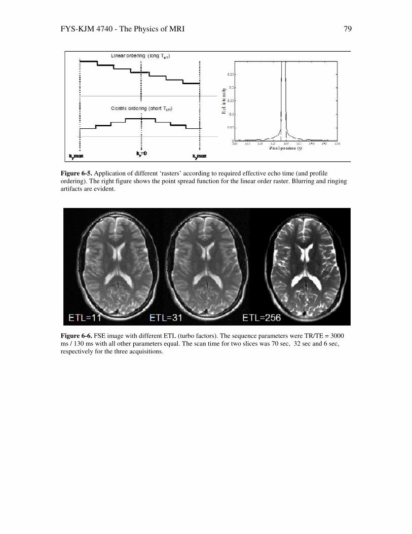
FYS-KJM 4740 - The Physics of MRI 79
Figure 6-5. Application of different ‘rasters’ according to required effective echo time (and profile ordering). The right figure shows the point spread function for the linear order raster. Blurring and ringing artifacts are evident.
Figure 6-6. FSE image with different ETL (turbo factors). The sequence parameters were TR/TE = 3000 ms / 130 ms with all other parameters equal. The scan time for two slices was 70 sec, 32 sec and 6 sec, respectively for the three acquisitions.

FYS-KJM 4740 - The Physics of MRI 80
Figure 6-7. Effect of T2-blurring in FSE sequences with long echo train length (ETL). In the right image (ETL=256) significant blurring is visible in the phase encoding direction. The effect is less evident in the left image (ETL=11).

FYS-KJM 4740 - The Physics of MRI 81
6.2. Echo Planar imaging (EPI)
Echo Planar imaging is conceptually very similar to FSE; the main difference
being that in EPI sequences gradient echo refocusing is used, rather than RF-refocusing. An EPI sequence is therefore essentially a way of accelerating the GRE sequence by acquiring multiple k-lines following a single excitation pulse. Since a gradient echo can be generated in a millisecond on modern scanners, a complete EPI image may be acquired in less than 100 ms. The major advantage of EPI acquisitions is therefore speed. The price you pay for this speed is extreme sensitivity to field inhomogeneities and general sensitivity to many artifacts. Figure 6-8 shows the basic EPI sequence with rectilinear sampling of k-space. Note how the trajectory moves from one k-line to the next by applying short ‘blips’ of the phase-encode gradient. Using this scheme, the main echo (effective echo time) occurs half-way through the acquisition when ky=0 line is sampled.
Figure 6-8. The basic echo planar imaging (EPI) sequence. Multiple k-lines are acquired
following a single RF-excitation by applying short ‘blips’ of the phase-encode gradient.
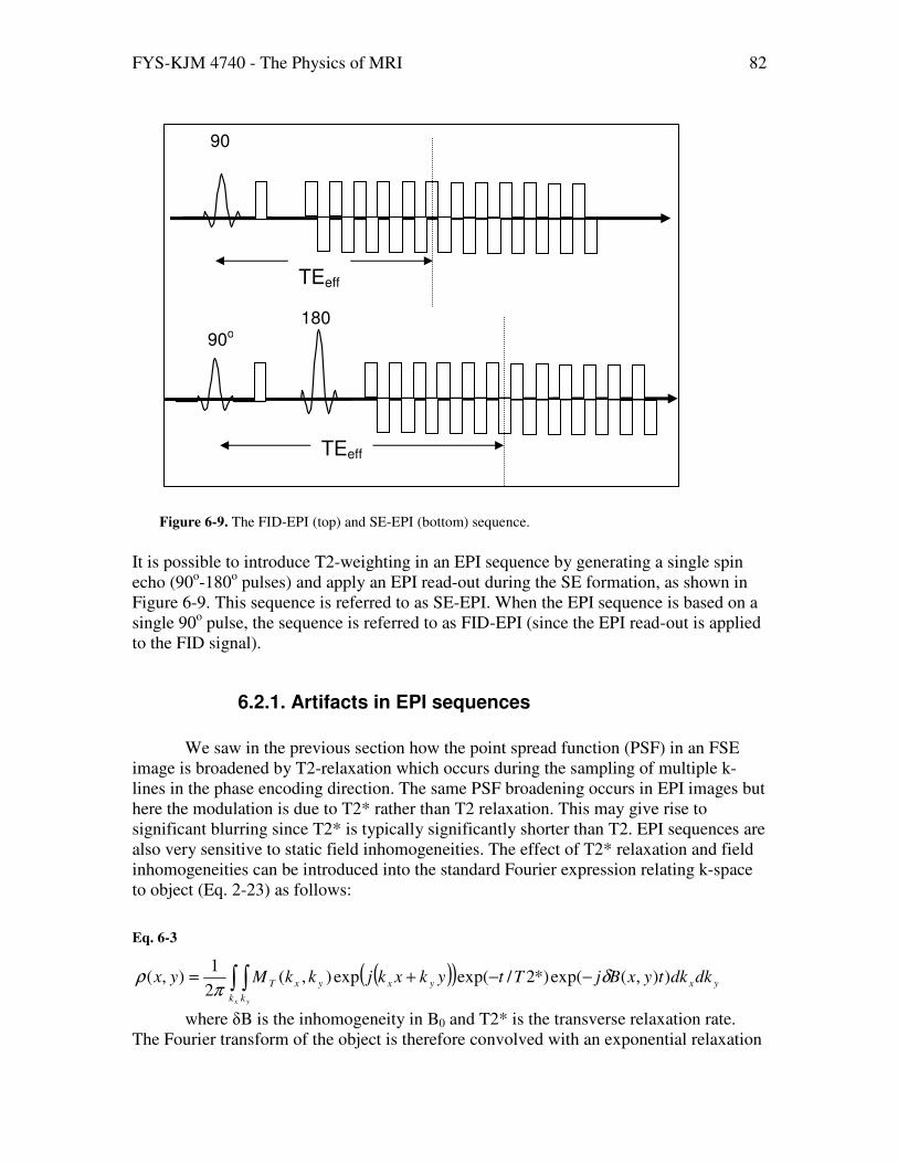
FYS-KJM 4740 - The Physics of MRI 82
It is possible to introduce T2-weighting in an EPI sequence by generating a single spin echo (90o-180o pulses) and apply an EPI read-out during the SE formation, as shown in Figure 6-9. This sequence is referred to as SE-EPI. When the EPI sequence is based on a single 90o pulse, the sequence is referred to as FID-EPI (since the EPI read-out is applied to the FID signal).
6.2.1. Artifacts in EPI sequences
We saw in the previous section how the point spread function (PSF) in an FSE
image is broadened by T2-relaxation which occurs during the sampling of multiple k-lines in the phase encoding direction. The same PSF broadening occurs in EPI images but here the modulation is due to T2* rather than T2 relaxation. This may give rise to significant blurring since T2* is typically significantly shorter than T2. EPI sequences are also very sensitive to static field inhomogeneities. The effect of T2* relaxation and field inhomogeneities can be introduced into the standard Fourier expression relating k-space to object (Eq. 2-23) as follows:
Eq. 6-3
( )( )∫ ∫ −−+=
x yk k
yxyxyxT dkdktyxBjTtykxkjkkMyx )),(exp(*)2/exp(exp),(2
1),( δ
πρ
where δB is the inhomogeneity in B0 and T2* is the transverse relaxation rate. The Fourier transform of the object is therefore convolved with an exponential relaxation
90o
90o 180o
TEeff
TEeff
Figure 6-9. The FID-EPI (top) and SE-EPI (bottom) sequence.

FYS-KJM 4740 - The Physics of MRI 83
term which causes blurring and an inhomogeneity term which causes spatial distortion. The relaxation term can be expressed in terms of the gradient strength by approximating the gradient to have an average value <G> so that k=γ<G>t. The PSF due to T2* is then given by:
Eq. 6-4
xTGj
TGTGk
*
2
*
2*
2
1
1/exp(
><+
><=><−ℑ−
γ
γγ
This is a Lorentzian with a FWHH given by:
Eq. 6-5
*)/(2 2TGx γ=∆
Due to the strong effective gradient in the read-out direction and short Tread, the
blurring due to finite sampling in the kx-direction is generally much larger than the blurring due to T2*; i.e. Tread << T2*. T2* blurring can, however be significant in the phase encode direction. The effect of reading out multiple ky-lines in a single sweep, can be considered in terms of a ‘pseudo-gradient’ in the ky-direction <Gy>. The velocity by which k-space is traversed in the ky-direction is much slower than in the kx-direction; which is to say that the effective gradient in the ky-direction is smaller than in the kx-direction. This k-space velocity can be defined as ky(t)=νyt and νy ≈ νx/N. The effective gradient is proportional to the average velocity so that:
Eq. 6-6
NGG xy /≅
where N is the matrix size in the read-out direction.
T2* blurring in the phase-encode direction from Eq. 6-5 is then given by:
Eq. 6-7
)/(2*
2TGNy xγ=∆
i.e. the FWHH in the phase-encode direction is N times larger than in the read-out
direction. Since the blurring due to finite sampling is the same in the x- and y-directions it is evident that T2* blurring can be a significant problem in the phase-encoding direction in EPI sequences.
The same line of argument can be followed for spatial distortions due to the field-inhomogeneity term in Eq. 6-3. These effects are also much more prominent in the phase-encode direction due to the much weaker effective gradient <Gy> compared to <Gx>. This is a particular problem in terms of water-fat shift, as will be discussed in more detail in Chapter 9.
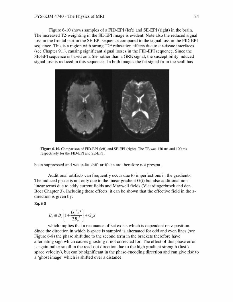
FYS-KJM 4740 - The Physics of MRI 84
Figure 6-10 shows samples of a FID-EPI (left) and SE-EPI (right) in the brain. The increased T2-weighting in the SE-EPI image is evident. Note also the reduced signal loss in the frontal part in the SE-EPI sequence compared to the signal loss in the FID-EPI sequence. This is a region with strong T2* relaxation effects due to air-tissue interfaces (see Chapter 9.1), causing significant signal losses in the FID-EPI sequence. Since the SE-EPI sequence is based on a SE- rather than a GRE signal, the susceptibility induced signal loss is reduced in this sequence. In both images the fat signal from the scull has
been suppressed and water-fat shift artifacts are therefore not present. Additional artifacts can frequently occur due to imperfections in the gradients.
The induced phase is not only due to the linear gradient G(t) but also additional non-linear terms due to eddy current fields and Maxwell fields (Vlaardingerbroek and den Boer Chapter 3). Including these effects, it can be shown that the effective field in the z-direction is given by:
Eq. 6-8
xGB
zGBB x
xz +
+≅2
0
22
02
1
which implies that a resonance offset exists which is dependent on z-position. Since the direction in which k-space is sampled is alternated for odd and even lines (see Figure 6-8) the phase shift due to the second term in the brackets therefore have alternating sign which causes ghosting if not corrected for. The effect of this phase error is again rather small in the read-out direction due to the high gradient strength (fast k-space velocity), but can be significant in the phase-encoding direction and can give rise to a ‘ghost image’ which is shifted over a distance:
Figure 6-10. Comparison of FID-EPI (left) and SE-EPI (right). The TE was 130 ms and 100 ms respectively for the FID-EPI and SE-EPI .

FYS-KJM 4740 - The Physics of MRI 85
Eq. 6-9
0
2
2B
NzGy x≅∆
Note that, for axial images, z is constant for a given slice. Complex methods exist to correct for these ghosting artifacts, but this is still an artifact which is commonly encountered in EPI images, especially in ‘single shot’ acquisitions. An example of this type of ghosting artifact is shown in Figure 6-11Figure 6-10.
Figure 6-11. Example of ghosting artifact in a single shot EPI image due to alternating
positive and negative phase errors in the rectilinear sampling scheme shown in Figure 6-8.

FYS-KJM 4740 - The Physics of MRI 86
6.3. Spiral imaging
Traditional EPI with rectilinear k-space trajectory places very strict demands on the gradient system since very rapid gradient switching is needed to cover k-space in a time comparable to T2* relaxation times in vivo. In an alternative approach k-space is covered in spiral trajectories running from the origin and outwards in k-space. The main advantage of spiral imaging approaches in that the path through k-space is very smooth, with consequent reduction in gradient switching demands. A second advantage is that the centre portion of k-space is densely sampled in a very short time after the excitation pulse is applied. Since image contrast is mainly determined by the centre k-space region, this means that spiral acquisitions are inherently quite insensitive for inhomogeneity and flow effects since these effects have little time to develop. The main disadvantage of spiral imaging is that k-space is not evenly sampled and the data points cannot be placed in a Cartesian grid, as required by the Foruier transformation method used to generate the MR image. The data points therefore need to be re-sampled (‘gridded’) into a Cartesian
coordinate system. Figure 6-12 shows a sample of a spiral k-space trajectory with two separate segments. The spiral trajectory (with constant increment per rotation) is given by:
Eq. 6-10
))(exp()()( 0ϕϕϕ jmtjtAt +=k
Figure 6-12. Spiral trajectories covering k-space as smooth spirals from the origin and outwards. Spiral imaging sequences usually cover k-space in multiple spiral segments as indicated in the figure.
kx
ky
kx
ky

FYS-KJM 4740 - The Physics of MRI 87
where φ(t) = tπ/N, φ0 is the initial angle of the first segment from the origin and m is the mth segment.
6.4. Further reading – Chapter 6
1. Vlaardingerbroek M, den Boer JA. Magnetic resonance imaging. Chapter 3.
Berlin: Springer; 1999 2. Listerud J, et al. First principles of fast spin echo. Magnetic Reson Quart (1992)
8(4):199-244. 3. Mansfield P and Maudsley AA. Planar spin imaging by NMR. J Magn Reson
1977;27:101-119. 4. Henning J et al. Clinical applications and methodological developments of the
RARE technique. Magn Reson Imaging 1988;6:391-395.

FYS-KJM 4740 - The Physics of MRI 88
7. Magnetisation preparation
In a spoiled GRE sequence, it was shown in Chapter 5.4.3 (Eq. 5-25) that, for TR << T1 and α>>αe the signal is proportional to TR/T1 The contrast (C=SI2-SI1) between two tissues with T1-values T1
2 and T11, respectively therefore scales with
TR(T12-T1
1)/(T11T1
2), as shown in Figure 7-1. Clearly, as TR gets very short little T1-contrast can be achieved and the contrast is mainly determined by the generally small difference in proton density between the tissues. This trade-off between speed (short TR) and good contrast is a common problem in many pulse sequences. A remedy to this problem is to ‘prepare’ the magnetization prior to the application of the pulse sequence. One common technique is to apply a 180o preparation pulse (or pre-pulse). The evolution of the longitudinal magnetization following an inversion (180o) pulse is given by:
Eq. 7-1
[ ])1/exp(21)( 0 TtMtM z −−=
Figure 7-2 shows the evolution of the signal (left figure) and the resulting
contrast between the same two tissues as simulated in Figure 7-1 as function of time after application of the inversion pulse. Notice that the SI in the MR image is assumed to be proportional to the modulus of the (complex) magnetization. It is usually (but not always) the case that MR pixel intensities are limited to positive values. This is referred to as an
Figure 7-1. Relative contrast between two tissue with T1 = 700 ms and T1 = 1000 ms in a spoiled GRE sequence as a function of TR for two different flip angles. The contrast decreases with decreasing TR, rendering short TR-images predominantly proton density weighted.
0 12.5 25 37.5 500
1
2
3
4
flip = 20 degflip = 50 deg
TR (ms)
Rel
Con
tras
t

FYS-KJM 4740 - The Physics of MRI 89
inversion recovery (IR) curve. If a 90o preparation pulse is used the corresponding signal curve is called saturation recovery (SR). Note that the use of an inversion pulse rather than a saturation pulse doubles the achievable contrast. The contrast obtained with such a preparation pulse is significantly larger than the native contrast in the short TR spoiled
GRE sequence if the optimal time after inversion time is used. If a preparation pulse is applied prior to e.g. a spoiled GRE acquisition, the signal will then mainly be determined by the value of the magnetization (due to the preparation pulse) at the time when the central part of k-space is acquired (see Chapter The k-space2.2). This is illustrated in the case of an inversion pre-pulse in Figure 7-4. Figure 7-3 shows examples of applying an inversion pre-pulse in a trueFISP sequence. The TI time was varied between 400 ms and 1500 ms, giving significant variations in the brain tissue contrast. Clearly, the optimal inversion time depends on the T1-times of the tissues of interest. For optimal grey/white matter contrast, an inversion time of about 900 ms is commonly used at 1.5 T. Contrast optimization is discussed in more detail in Chapter 8.
Magnetization preparation can in theory be applied to any pulse sequence where the acquisition time is short relative to T1-relaxation times. Clearly, if the acquisition time is several minutes then the preparation pulse will have little effect since the magnetization will return to its equilibrium value long before all data has been acquired. Even in long sequences, however, preparation pulses can be useful by splitting the sequence into segments of appropriate lengths and applying a preparation pulse prior to each segment. Consequently, preparation pulses are successfully applied also to 3D acquisitions whereby one inversion pulse is applied prior to the acquisition of each slice in the 3D volume. One such sequence is (by one vendor) called MPRAGE (magnetization prepared rapid gradient echo) which gives very good contrast resolution in the brain. An example of an MPRAGE image of the brain is shown in Figure 7-5.
Other types of preparations can also be applied, for instance a SE preparation (90o-180o pulse pair) if often applied in EPI sequence to introduce T2-contrast, as discussed in Chapter 6.2. In all cases, the signal is modulated by relaxation effects during the echo read-out; a situation similar to that described for FSE and EPI sequences
Figure 7-2. Relative signal (left) and contrast (right) obtained by applying a 180o inversion pulse at t=0
as a function of time for two tissues with T1 = 700 ms and T1=1000 ms, respectively.
0 500 1000 15000
50
100
T1=700 msT1=1000 ms
Time after inversion pulse (ms)
Rel
ativ
e si
gn
al
0 500 1000 150040
20
0
20
40
Time after inversion pulse (ms)
Rel
ativ
e co
ntr
ast

FYS-KJM 4740 - The Physics of MRI 90
Chapter 6. Consequently, magnetization preparation may lead to blurring and ringing artifacts if the relaxation times (T1- or T2-, depending on type of preparation) is short relative to the acquisition window.
Note that we in this discussion assume that a steady state condition is reached when the inversion pulse was applied. This may (for GRE sequences) imply that multiple dummy pulses have to be applied prior to application of the preparation pulse.
Figure 7-3. The effect of varying the inversion time (TI) in a trueFISP sequence (TR/TE/flip = 4 ms/2 ms/70 deg). The inversion times were (left-right) 400 ms, 700 ms, 900 ms and 1500 ms. Note the distinct change in
grey/white matter contrast as a function of TI.
0 500 1000 15000
50
100
T1=700 msT1=1000 ms
Inversion time (TI, ms)
Rel
ativ
e si
gnal
Tacq
TI
Figure 7-4. The application of a inversion pre-pulse to increase contrast in a rapid sequence. The actual sequence is acquired in the time-window, Tacq , and the time from the application of the inversion pulse to the centre of the acquisition window is called the inversion time (TI).

FYS-KJM 4740 - The Physics of MRI 91
7.1. Selective tissue suppression
Pre-pulses are often used to selectively suppress the signal from certain tissues.
From Figure 7-4 it is evident that the signal can be virtually eliminated by selecting the appropriate TI-value for a given target T1. The optimal TI-value to null the signal from a given tissue T1 can readily be obtained from Eq. 7-1:
Eq. 7-2
11 69.0)2ln(
0)1/exp(21
TTTI
TTI
⋅==
=−−
Inversion pre-pulses are commonly used to suppress signal from fat or
cerebrospinal fluid (CSF). Figure 7-6 shows an example where CSF is suppressed using an inversion pulse with a TI of 2500ms (right image). This sequence is called FLAIR (Fluid Attenuated Inversion Recovery) and is very useful for detection of small lesions (like multiple sclerosis plaques or tumors) in the close vicinity of the ventricles in the brain. In a normal T2-weighted FSE sequence both CSF and many lesions will appear hyper-intense and are therefore hard to differentiate. Increased lesion conspicuity can then be achieved by selectively suppressing the signal from CSF - based on the longer T1-value.
Figure 7-5. The MPRAGE sequence which is a fast 3D-acquisition with in inversion recovery (IR) preparation pulse. An inversion time of 900 ms was used, which gives good grey-white
matter contrast.

FYS-KJM 4740 - The Physics of MRI 92
7.2. Influence of excitation pulses on the magnetization curve
In the previous section we discussed how tissue with a given T1 can be selectively
suppressed by using an inversion pulse with the appropriate TI so that the tissue magnetization passes through zero when the centre of k-space is reached. In the calculation of the ‘zero-crossing’ TI value (Eq. 7-2) we assumed that the magnetization recovery following the pre-pulse is unaffected by the excitation pulse of the actual sequence used to acquire the data. In reality, the magnetization recovery will be affected by the excitation pulses for all flip angles > 0 degrees. Clearly, the effect of the pulses will be greater with increasing flip angle since this will cause a greater disturbance in the longitudinal magnetization vector. It can be shown that the ‘apparent’ T1-relaxation under the influence of excitation pulses with flip angle α is given by:
Eq. 7-3
))ln(cos(11
α−=T
TR
T
TR
app
Figure 7-7 shows how the deviation from the true magnetization recovery curve
increases with increasing flip angle. This correction is important both for determining the optimal TI-value for signal suppression.
Another situation where this correction is of importance is when attempting to quantify T1-relaxation based on probing of the recovery curve. This is a common approach to measuring T1-values. Following an inversion pre-pulse, multiple very rapid acquisitions are acquired at different time-points during the recovery phase (or segmented across several inversion pulses). A correction in the measured T1-values must then be
Figure 7-6. Comparison of T2-weighted FSE (left) and FLAIR (fluid attenuated inversion recovery) (right). The FLAIR sequence uses an inversion pulse with a TI of 2500 ms (at 1.5 T) which
effectively suppresses signal from the CSF, leaving small peri-ventricular lesions more conspicuous.

FYS-KJM 4740 - The Physics of MRI 93
applied according to Eq. 7-3 in order to obtain the ‘true’ T1-relaxation times and the smallest possible flip angle should be used as shown in Figure 7-7. Note, however, that a very small flip angle also reduces the signal-noise ratio, which tend to limit how small flip angles can be used in practice. Also, the flip angle is not equal to the nominal value at all points in the excited slice or volume due to imperfect excitation profile (see Chapter 2.1) which may also limit the minimum flip angle.
Figure 7-7. The effect of excitation pulses in a T1-GRE sequence on the magnetization recovery curve following an inversion (180 deg) pulse. The simulation was performed with T1=900 ms and TR=10 ms. The first RF-pulse of the GRE sequence is applied at t=0, but was preceded by multiple dummy pulses to assure that steady-state conditions. The ‘flip=0’ curve (crosses) indicate the true undisturbed recovery curve. The increasing deviation from the true inversion recovery curve with
increasing flip angle is evident.
0 500 1000 1500 2000 2500 3000 3500 4000 4500 5000-50
-40
-30
-20
-10
0
10
20
time (ms)
Mz
(a
.u.)
flip=30
flip=0
flip=10
flip=3

FYS-KJM 4740 - The Physics of MRI 94
8. Image quality, signal, contrast and noise
Like in most aspects of life, nothing comes for free in MRI, and sequence optimization is a constant trade-off between parameters acting in ‘opposite’ directions. For instance, let’s say you want to increase image resolution in order to better see a specific detail in your MR image. Increasing resolution, however, causes a reduction in the signal to noise ratio (SNR) which offsets the gain in resolution. You may then want to try and compensate for the reduced SNR by changing some image parameter, e.g. increasing TR but this may reduce the contrast between the detail of interest and surrounding tissue and in spite of all your efforts you still cannot see the detail of interest any better. Image optimization in MRI is clearly a multi-dimensional problem.
We can think of this trade-off as a rectangle where different MR parameters try and move different corners of the rectangle in different directions but the total area of the rectangle must be kept constant for a given MR-scanner (Figure 8-1). One can then think
of the size of the box as the overall quality or performance of a given scanner (large box = good scanner). In this chapter we will discuss the four different ‘corners’ of the box and the parameters inside that we can use to optimize our MR image.
8.1. Signal versus noise
It is well known from electromagnetic theory that an alternating magnetic field
will induce a current in a coil exposed to the field and that the resulting signal in the coil
contrast SNR
speedresolution
Available MR-
parameters
contrast SNR
speedresolution
Available MR-
parameters
Figure 8-1. The optimization problem in MRI. The area of the box is fixed for a given scanner and a given object to be scanned.

FYS-KJM 4740 - The Physics of MRI 95
is proportional to the frequency of the magnetic fluctuation and the number of turns, N, making up the coil: S(t)=KNω0MT(t), where K=constant and MT is the fluctuating magnetization vector.
If initially we ignore the influence on SNR of imaging parameters and tissue relaxation properties, the signal induced in the receiver coil with N turns is then given by
Eq. 8-1
)())(exp()()( 0 tndrrtjkrMNtSv
T +−= ∫ω
where n(t) =nr(t) + jni(t) is the complex noise term. Comparing this expression to Eq. 2-23 we see that k(t) is the usual k-space trajectory function, and the object spin distribution can be obtained by Fourier transformation of the detected signals with varying gradients as discussed in Chapter 2.2 It can be shown (Macovski A. MRM 36:494-497 (1996)) that the noise-independent part of the estimated MR signal from a voxel of volume Vh is given by:
γχω /2
0 hsig VNM =
and the signal-noise ratio (SNR) is given by:
Eq. 8-2
r
h
TRkT
VNSNR
/2
2
0
⋅=
χω
where k is the Boltzmann’s constant and T is the temperature in Kelvin, Tr is the read-out time (time used to record the echo signal), R is the coil resistance and N is the number of coil turns and Vh is the voxel volume. From this expression it appears that the SNR scales with the square of the magnetic field strength and with the number of coil turns. This is the SNR for a single voxel but any imaging experiment consist of more than one voxel and hence many repeated experiments. Further, it can be shown that the coil resistance R is a complex function of field strength and a more realistic estimate of SNR in a single 2D slice is given by:
Eq. 8-3
BW
QBNVASNR
y
h
3
0⋅=
where A is a constant (product of all relevant physical constants like susceptibility and temperature, as well as object geometry and size), Q is the quality factor of the coil = ωL/R (L=coil inductance and R=resistance) and BW is the bandwidth = 1/Tr. The main importance for our discussion is that SNR is proportional to voxel volume and to the square root of the total acquisition time. The exact dependence of field strength on SNR is more uncertain due to the dependence of coil resistance on B0.

FYS-KJM 4740 - The Physics of MRI 96
We now need to consider the influence of sequence parameters, acquisition method and tissue relaxation properties on the SNR. The use of 3D acquisitions was discussed in Chapter 4.3.2 whereby the entire volume of interest is non-selectively excited by each RF-pulse and a second phase encoding gradient is applied in the slice direction. We can think of this as an extension of k-space by a third dimension. From this it follows that the SNR scales with the square root of the number of 3D-slices as well as with the number of phase encoding stems (both 2D and 3D). We also need to include the effect of multiple averages, which is commonly used in practice if SNR is marginal and acquisition time is not critical. Repeating the whole image acquisition N times increases SNR by √N. If quadrature coils are used the SNR increases by √2 since two independent signals (one shifted 90o in phase relative to the other) are effectively generated.
Finally, SNR is clearly influenced by the type of pulse sequence used, tissue
relaxation properties and sequence parameters. The signal behaviour of different sequences was discussed in Chapters 4 and 5 and the signal response of a pulse sequence is in general a function of TR, TE, flip angle as well as the biophysical properties of the tissue; T1, T2, T2* and proton density. The grand total SNR is then given by:
Eq. 8-4
)T2*, T2,T1,,TE,S(TR,
3
0ρα⋅
⋅⋅= h
sySAV
BW
NNNQBASNR
where NSA = number of averages, Ny = number of phase encoding steps,
Ns=number of 3D slices (=1 for 2D acquisitions) and S is the sequence dependent signal response. S needs to be determined specifically for the pulse sequence in question and we shall show some specific examples in the next section. Note that the sources of noise discussed so far are assumed to be position independent in the image. There are additional sourced of noise which are position dependent; e.g. due to respiration and physiological motion, flow, susceptibility effects etc.
8.2. Signal versus contrast
Although a highest possible SNR is generally desirable, it is not going to be of
any help if the contrast between adjacent image structures is poor, and in practical imaging it is the contrast-noise ratio (CNR) which needs to be optimized. The CNR can be defined as follows:
Eq. 8-5
σ
)()( BSASSNRSNRCNR BA
−=−=

FYS-KJM 4740 - The Physics of MRI 97
where S(A,B) is the signal in points A and B, respectively and σ is the image noise. Note that we assume the noise to be position independent.
We discussed in Chapter 4 how the signal in GRE sequences could be optimized by selecting the correct flip angle as a function of TR, T1 and T2. It should be noted that optimized signal is not equivalent to optimized contrast. As an example, let’s consider the spoiled gradient echo sequence given in Eq. 4-9 and look at the difference between peak signal and peak contrast. Figure 9-2 shows the signal response and relative CNR between two tissues (T1 = 900 ms and 300 ms) as a function of flip angle (T2* effects are assumed to be negligible). We note that the optimal CNR is obtained at a higher flip angle than the Ernst angle for the shortest T1-value.
We can similarly determine the optimal TR in SE sequences for optimal CNR if the target T1 values are known. Assuming T2-effects to be negligible (T1-weighted) we can easily derive the optimal TR by taking the derivative of the signal difference using the standard SE signal equation. We then get:
Eq. 8-6
)1/1ln(11
1121
21
21 TTTT
TTTRopt ⋅
−=
0 25 50 75 1000
0.05
0.1
0.15
0.2
0.25
T1=900T1=300
CNR
Flip angle (deg)
Rel
SI,
Rel C
NR
0 25 50 75 1000
0.05
0.1
0.15
0.2
0.25
T1=900T1=300
CNR
Flip angle (deg)
Rel
SI,
Rel C
NR
Figure 8-2. Relative signal level in spoiled GRE sequence (TR=30 ms) for two different T1-values as function of flip angle. The thick dotted line shows the relative contrast-noise ratio (CNR). Note that flip
angle for optimal CNR is higher than the Ernst angle for the shortest T1.

FYS-KJM 4740 - The Physics of MRI 98
Note that Eq. 8-6 also is also the expression for optimal inversion time (replacing TR with TI) in a magnetisation prepared rapid sequence (with either a saturation- or inversion recovery preparation pulse), as discussed in Chapter 7.
8.3. Practical measurements of SNR and CNR
In practice, the noise in an MR image is estimated from the variance of the signal
in an ‘empty’ region of the image; i.e. the variance in air, as shown in Figure 8-4. It is important to use the variance of the background signal and not its mean value. In an ideal case of Gaussian white noise, mean value should be zero and the noise should therefore include both positive and negative values (since the noise is a complex property). However, since the absolute value of the complex MR signal is displayed, the negative noise values are mirrored around the mean value of zero which shifts the mean level to a positive value. The variance of the noise is, however, not affected by this. Note that the background signal may often appear completely homogeneous (black) and ‘noisless’. This is due to the window scaling of the image and if the image contrast and intensity is turned up (right image in Figure 8-4) the image noise will be apparent. Figure 8-5 shows the effect on SNR of increasing number of signal averages in a single shot echo planar (EPI) acquisition. The SNR increases with √NSA, as expected from theory.
Figure 8-3. Relative signal in SE sequence as function of TR for two different T1
values and the corresponding CNR (dotted line).
0 200 400 600 800 10000
0.5
1
1.5
T1=900T1=300
CNR
TR (ms)
Rel
sig
nal
, re
l C
NR
0 200 400 600 800 10000
0.5
1
1.5
T1=900T1=300
CNR
TR (ms)
Rel
sig
nal
, re
l C
NR

FYS-KJM 4740 - The Physics of MRI 99
The effect of pixel bandwidth on SNR is shown in Figure 8-6. As expected from theory, the variance of the noise scales with √BW and hence SNR scales with 1/√BW.
Sa Sb
σ2
Sa Sb
σ2
Figure 8-4. Practical measurement of SNR and CNR. The image noise is measured from the variance
of the signal in an empty (air-filled) region of the image.

FYS-KJM 4740 - The Physics of MRI 100
0
5
10
15
20
2 5
0 5 10 15 2 0 25
N umb e r o f ave rag e s
0
5
10
15
20
2 5
0 5 10 15 2 0 25
N umb e r o f ave rag e s
Figure 8-5. The effect of increasing number of averages (NSA=1,5 and 10).
The SNR increases with the square root of NSA, as expected from theory.
Figure 8-6. The effect of pixel bandwidth (BW) on SNR in a single-short SE-EPI sequence. The BW was 750 Hz and 2055 Hz in the left and right image respectively. All
other parameters were kept constant. As expected the noise variance scaled with √BW.

FYS-KJM 4740 - The Physics of MRI 101
8.4. Partial k-space sampling
For most types of sequences the scan-time is proportional to the number of phase-
encoding steps and an obvious way to reduce scan-time is therefore to reduce Ny, at the cost of reduced SNR. In many cases, the symmetrical properties of k-space can be used to reduce Ny without reducing the spatial resolution in the y-direction.
Since the applied gradients Gx,y take on both positive and negative values the sign of kx,y changes when the trajectory passes the centre row / column in k-space and the magnetization vector at any point in k-space can be expressed as the complex conjugate of the magnetization in the opposite quadrant (Figure 8-7, left image). This symmetry is clearly visualized in the k-space representation of an MR-image shown in Figure 2-3. This means that, theoretically (if the symmetry was perfect) only half of k-space needed to be sampled in order to determine the complete magnetization matrix. In practice, perfect symmetry is not possible due to phase errors introduced by many different sources (field inhomogeneities, eddy currents etc) so that slightly more than half of k-space needs to be sampled to properly reconstruct the image. Two different schemes are used for partial k-space sampling; depending on whether the phase-encode direction or the frequency-encode direction is partially sampled. The two different schemes are shown schematically in Figure 8-7 and will be discussed separately below.
8.4.1. Partial echo acquisition
In partial (also called fractional or asymmetric) echo acquisitions, only the last part of the echo is sampled, as shown in Figure 8-8. The main advantage of this approach is that the echo time can be reduced, since the duration of the negative lobe of Gx can be made shorter. Or, in the case of a SE sequence, the 1800 pulse can be moved closer to the 900 pulse therefore reducing TE. The reduced sampling of the echo reduces SNR, where the actual reduction depending on the approach used to fill in the missing part of k-space.
The simplest approach is to simply zero fill the missing data. This is not a feasible approach since it introduces an abrupt change in k-space where the data is missing giving
kx
ky
p1
p*1
p2
p*2
A B
Figure 8-7. Partial k-space sampling can be applied either in the frequency encoding direction (A) or in the phase encoding direction (B).

FYS-KJM 4740 - The Physics of MRI 102
rise to severe ringing artefacts. These artefacts can be reduced by applying a smoothing kernel to the early part of the sampled echo. This reduces ringing artefacts at the expense of resolution. The final approach is to obtain the missing data points from the complex conjugates of the sampled points. This eliminates ringing artefacts.
The SNR scales approximately with √PEF where PEF is the fraction of the echo
which is sampled The exact SNR loss does, however, depends to some extent on which of the approaches discussed above is used to fill in the missing data.
8.4.2. Reduced matrix acquisition
Reducing the number of ky-lines, Ny, is a common approach to reducing scan-
time. The effect in the image of reducing Ny depends on which k-lines are left out and how we deal with the part of k-space not sampled. A similar approach to the partial echo technique described above can be applied in the phase encoding direction. This approach is called partial Fourier or half-scan (Figure 8-7 B). The unsampled part of k-space is typically zero filled and the spatial resolution is not affected.
In an alternative approach referred to as rectangular field of view (rFoV) the sampling frequency is decreased in the phase encoding direction. In other words, the
‘distance’ between adjacent ky-lines is increased and a given k-space distance in the y-direction is covered with fewer phase encoding steps (Figure 8-9). The last approach is to simply acquire fewer ky-lines without changing the distance between the lines. This reduces the resolution in the y-direction. Note that, for all three techniques, SNR scales with √Ny.
α
TE
α
Tacq
TE
Tacq
Gx
A B
Figure 8-8. Full echo (A) and partial (fractional) echo technique (B) used to reduce the minimum TE

FYS-KJM 4740 - The Physics of MRI 103
8.5. Further reading – Chapter 8
1. Vlaardingerbroek M, den Boer JA. Magnetic resonance imaging. Chapter 6. Berlin: Springer; 1999
2. The physics of MRI. American Association of Physicists in Medicine Medical Physical Physics Monograph No. 21. 1992 AAPM Summer School Proceedings.
3. Macovski A. Noise in MRI. Magn Reson Med (1996) 36:494-497
kyky
Figure 8-9. Reducing the ‘sampling rate’ in the phase-encode direction means that the same ‘distance’ along ky can be covered with less phase encoding steps. This results in a reduced field of view in the y-direction in the
image and is referred to as rectangular FoV (rFoV)

FYS-KJM 4740 - The Physics of MRI 104
9. Off-resonance effects
In this chapter we will discuss the effects of deviations in the static magnetic field from its nominal B0-value – collectively referred to as off-resonance effects. There are two main sources of off-resonance effects in MRI; namely susceptibility effects and chemical shift effects. Chemical shift is due to the difference in resonance frequency between water and fat. This difference is 3.5 ppm, which implies a frequency difference of about 220 Hz at 1.5 T. Magnetic susceptibility differences can also cause offsets in the resonance frequency as will be discussed in more detail below. Whereas chemical shift can cause spatial displacement of the fat signal, susceptibility effects can give rise to more complex geometric distortions as well as signal loss. However, the physical cause of the distortions is in both cases local deviations in the static field and it is therefore appropriate to discuss these effects in the same chapter. Since magnetic susceptibility is a rather complex effect it will be discussed in some more detail below.
9.1. Magnetic susceptibility
The relationship between applied magnetic field B0 and induced nuclear
magnetization was discussed in Chapter 1.The induced magnetization can be written in terms of the nuclear susceptibility, χ:
Eq. 9-1
00/ HBM 0 χµχ ==z
where H0 is the induced magnetic field and µ0 is the permeability of free space (=4π x 10-7 H/m). Note the distinction between magnetic field H with units of A/m and magnetic flux density B with units of Tesla. The magnetic field density B is commonly referred to as the ‘field strength’ in the MRI literature and it should be noted that B is really the magnetic induction, which is proportional to the magnetic field M. Comparing Eq. 9-1 with Eq. 1-3 the nuclear susceptibility is equal to:
Eq. 9-2
Tk
uN
Tk
IIN
B
z
B 33
)1( 0
2
00
22
0 µµγχ =
+=
h
where u is the magnetic moment per atom. It is important to distinguish between
nuclear susceptibility of the proton which is paramagnetic (χ >0) and the bulk susceptibility of tissue which is diamagnetic (χ <0). The nuclear susceptibility is very small due to the small magnetic moment of the nucleus and the total susceptibility of tissue (water) is therefore completely dominated by the much larger diamagnetic effect. The effective local magnetic field is then given by:

FYS-KJM 4740 - The Physics of MRI 105
Eq. 9-3
0)1( BBeff χ+=
The effective field is therefore smaller than the applied field in a diamagnetic medium and larger than the applied field in a paramagnetic medium. Note that for all biological tissues, both diamagnetic and paramagnetic, | χ| << 1. Table 9-1 gives the susceptibility for a selection of materials. Note that, although the in vivo susceptibility may vary up to +/- 2 ppm, most biological tissues have susceptibility within 1 ppm of the value for water. As an interesting side-comment; the susceptibility of a superconducting media is χ=-1 which means that any applied field is completely cancelled inside the superconductor.
Material Susceptibility (x 106)
Water -9.63
Human tissues ≈ -11 to -7
Whole blood (deoxygenated) -7.9
Whole blood (oxygenated) -9.6
Air +0.36
Ferritin +520
Liver with severe iron overload
≈ 0
Iron +200 000
Gadolinium +0.32
Table 9-1. Susceptibility (in ppm SI units) for selected materials (from Schenk JF, Med Phys 23(6):1996)
9.1.1. Diamagnetism
In a magnetic field, the orbital motion of the electrons is slightly modified and according to Lenz’s law induces a change in motion creates a magnetic field which opposes the applied field. This effect occurs in all materials and is called Langevin diamagnetism. The diamagnetic susceptibility is given by:
Eq. 9-4
e
dm
rnZe
6
22
0µχ −=
where n is the number of atoms per unit volume, Z is the number of electrons per
atom, e is the electronic charge, me is the electronic mass and <r2> is the root mean square atomic ratio (typically 10-21 m2). The bulk susceptibility of human tissues is almost always negative (due to high water contents); except possibly in some extreme cases of e.g. iron overload of the liver. Diamagnetic susceptibility is essentially independent of temperature but a function chemical structure; a dependence which is

FYS-KJM 4740 - The Physics of MRI 106
utilized in NMR spectroscopy. Note that χ is unitless (or given in parts per million, ppm) when expressed in SI units.
9.1.2. Paramagnetism
There is another type of paramagnetism (in addition to nuclear paramagnetism), called Curie paramagnetism which is due to unpaired electrons in the outer orbital shells of an atom. Curie paramagnetism is a much stronger effects than nuclear paramagnetism because the magnetic moment of the electron is much larger than that of the nucleus. The Curie paramagnetic susceptibility is given by:
Eq. 9-5
Tk
Nm
B
p3
0
2µχ =
where m is the magnetic moment of the unpaired electrons and N is the number of
atoms per unit volume. Paramagnetism is an important property in MRI for several reasons. First,
exogenous paramagnetic agents can be used (i.e. injected into the patient) to alter the relaxation properties of tissue. Most MR contrast agents are paramagnetic and their application will be discussed in more detail in Chapter XXX. Further, certain biological tissues can have paramagnetic properties which can give rise to large local variations in magnetic susceptibility. These susceptibility variations can have significantly influence MR image contrast and quality. Paramagnetic substances present in the body include air (e.g. air filled cavities in the lung and brain), deoxygenated blood (paramagnetic iron in hemoglobin) and ferritin/ hemosiderin (blood breakdown products). Even in the presence of paramagnetic substances, the overall susceptibility of all tissues are still diamagnetic (except in some rare cases; see Table 1) due to the high concentration of diamagnetic water in all living tissues. Even though tissues as a whole are diamagnetic, local susceptibility differences can be significant and may give rise to significant imaging effects. As an example the difference in susceptibility between oxygenated and deoxygenated blood (about 2 ppm) is utilized in functional MRI to visualize focal brain activation thought the so-called BOLD (Blood Oxygen Level Dependent) effect.
9.2. Implications for imaging
It is clear that differences in local tissue susceptibility can have profound effects
in the MR image since the spatial encoding of the MR signal is dependent on a homogeneous and well controlled magnetic field. In MR nomenclature, the (adverse) imaging effects caused by local variations in susceptibility of are commonly referred to as ‘susceptibility effects’. It would be more accurate to refer to them as ‘susceptibility difference effects’.

FYS-KJM 4740 - The Physics of MRI 107
The effects of field inhomogeneities depend on the extent of the field perturbation relative to the pixel dimensions (or pixel bandwidth) (see Figure 9-1). If the perturbation occurs over a small distance relative to the voxel size an increase in the transverse relaxation will occur due to increased phase dispersion within the voxel volume. This effect is referred to as intravoxel dephasing. If the field perturbation occurs over a large distance relative to the voxel dimension then signal mis-registration occurs since the field in a given voxel can then be approximated to be constant but shifted up or down from its reference value (given by the Larmor frequency). This is referred to as off-resonance effects. The overall susceptibility effect is generally a mix of intravoxel dephasing and off-resonance effects.
9.2.1. Intravoxel dephasing – signal loss
The effect of intravoxel dephasing occurs when the phase dispersion due to field
inhomogeneities within a voxel is large compared to the phase induced by gradients used to encode the image. This is equivalent to saying that effective read-out time for a given voxel dimension must be short relative to the effective transverse relaxation rate. The
Figure 9-1. Two different susceptibility effects; intravoxel dephasing (top), which leads to signal loss and off-resonance effects (bottom) which leads to geometrical distortion and signal displacement. The extent to which each effect occurs depends on the voxel dimensions relative to the extent of the
field perturbation.
∆B pixel
∆B
pixel

FYS-KJM 4740 - The Physics of MRI 108
signal decay from a voxel due to phase variations can in general be expressed in terms of the Fourier transform of the phase distribution according to:
Eq. 9-6
∫ ⋅=voxel
drrjrS ))(exp()( ϕρ
where φ(r) is the position dependent phase shift within the voxel due to field inhomogeneities. If we assume a linear range of frequencies within a voxel from –∆ω to ∆ω, the total signal from a cubic voxel with constant spin density is given by:
Eq. 9-7
33
)sin()/exp()(
1)(
∆
∆=
∆⋅= ∫
−TE
TEdrdrTEjr
dTES
d
dω
ωωρ
The resulting signal decay as function of TE (for a given ∆ω ) is shown in Figure 9-2. In reality, the signal dephasing due to intravoxel dephasing is usually well approximate by a single exponential which implies that the field distribution within a voxel is Lorentzian rather than linear.
It is important to note that intravoxel dephasing can be completely rephrased in a SE sequence (due to the 180o pulse) if the effect of water diffusion is small. This condition is referred to as static dephasing. In other words, if the water protons within a voxel experience a constant field on a time-scale equal to the echo time then intra-voxel
dephasing does not occur in a SE sequence. This re-phasing does not occur in GRE
5 10 15 200
0.5
1
Echo time (ms)
Rel
ativ
e si
gnal
Figure 9-2. Signal decay due to intravoxel dephasing in a GRE sequence for a linear frequency distribution within a voxel.

FYS-KJM 4740 - The Physics of MRI 109
sequences, as discussed briefly in Section 1.3.2 and these sequences are therefore always sensitive to intravoxel dephasing. This is the reason why the effective transverse relaxation rate, 1/T2*, experienced in a GRE sequence is always higher than the rate experience in a SE sequence. Figure 9-3 shows the additional T2* relaxation due to intravoxel dephasing in a spoiled GRE image (left image) compared to in a SE image (right), using the same TE. Note the much larger signal loss in the GRE sequence in the regions with air-tissue interfaces. Due to the large difference in susceptibility between air and tissue (see Table 9-1), intravoxel dephasing effects can be problematic in these regions.
9.2.2. Off-resonance effects – geometric distortions
If the voxel dimension or voxel bandwidth is small relative to the spatial extent of the field perturbation then off-resonance effects may be the dominating susceptibility effect. This is because the field variation within a single voxel is then small but the entire voxel may experience a frequency offset. With this assumption the field offset of a given voxel adds to the effective field in the z-direction. Including the applied gradient, the total z-component of the field is then given by:
Eq. 9-8
),,()()(0 zyxBytGxtGBB zyxz ∆+++=
Figure 9-3. The effect of intravoxel dephasing in the region of the sinuses (arrows). Note the larger signal loss in
the Spoiled GRE image (left) compared to the SE image (right). An echo time of 15 ms was used in both images.

FYS-KJM 4740 - The Physics of MRI 110
where ∆Bz(x,y,z) is the total field produced by the magnetization of the patient (≈ χB0). In order for ∆Bz to be negligible, the field variation induced by the encoding gradients must be much larger than the field offset due to patient magnetization. On important comment should be made here. For conventional GRE and SE sequences, spatial distortions will always occur along the frequency encoding direction (e.g. along the read-out gradient). This is because the phase offset due ∆Bz in the phase encoding direction is a constant for all phase encoding steps and therefore does not introduce any time-varying (and hence position sensitive) modulation of the signal. This is NOT the case for EPI acquisitions where the entire k-space is covered in a very short time. Off-resonance effects in EPI sequences will be covered in a separate section.
The magnitude of the spatial distortion due to ∆Bz can now be expressed in terms of the applied read-out gradient strength as follow:
Eq. 9-9
xGBx /0χ∆=∆
where ∆x is shift in pixel orientation along the read-out gradient with peak magnitude Gx
due to a susceptibility induced field shift ∆χB0. The pixel dimension in the read-out direction (see Section 3.1) is given by:
Eq. 9-10
sxx tNGx
γ
πδ
2=
where Nx is the matrix size (number of pixels) in the x-direction and Nx.ts is the total
read-out time = Tread. In order to have a negligible pixel shift we must then have ∆x << δx or:
Eq. 9-11
0
2
BTread
χγ
π
∆<<
In other words, the pixel bandwidth (BW=1/Tread ) must be large relative to the susceptibility induced frequency shift γ∆χB0. There are many ways in which the pixel bandwidth can be increased; for instance by a) increasing the gradient strength Gx or b) reducing the image resolution (larger field of view or smaller image matrix). Note, however that increasing the bandwidth by increasing the gradient strength causes a reduction in the SNR since SNR is proportional to 1/√BW. Reducing the resolution does not generally reduce the SNR (for a constant gradient strength) since the resulting reduction in SNR due to reduced BW is offset by the increase in SNR due to the larger voxel size. Increasing the voxel size does, of course reduce image resolution and might therefore not be an acceptable solution. Also, increasing the voxel size may increase intravoxel dephasing (larger ∆ω in Eq. 9-7).

FYS-KJM 4740 - The Physics of MRI 111
We can from this conclude that, for a given field perturbation (that cannot be removed) we often will have to chose between geometric distortion (off-resonance
effects) or signal loss (intravoxel dephasing) but can generally not avoid both. The actual effect in the image of off-resonance effects is a complex function of geometry of the different compartments having different χ. It can, however, be constructive to assess the effect of standardized geometrical shapes on image distortion since many biological structures can be reasonably approximated by simple shapes. It may, for instance be reasonable to model blood vessels as infinite cylinder and red blood cells as spheres or ellipses. The field distribution due to both cylinders and spheres can be determined analytically, and the effects in the image can therefore also be modeled with good accuracy.
The field inside an infinite cylinder with its long axis perpendicular to B0 is given by ∆Bz,i=∆χB0/2 where ∆χ is the susceptibility difference between the interior and the exterior of the cylinder. The field distribution outside the cylinder of radius R is given by:
Eq. 9-12
222
222
,,)(
)(
xz
xzRBB izoz
+
−∆=∆
Interestingly, if the cylinder is oriented with its long axis parallel to B0 then ∆Bz,i= ∆χB0 and ∆Bz,o=0; i.e. the cylinder has no effect of the external field. This immediately indicates the complexity of modeling any real biological system. Figure 9-5 shows the field distribution due to a cylinder parallel to B0 according to Eq. 9-12. Note the large field perturbations occurring at the cylinder surface. Once the field distribution is known its effect in the image can readily be calculated.
B0
Figure 9-4. Magnetization distribution induced by difference in susceptibility ∆χ between the inside and outside a cylinder oriented perpendicular to B0.

FYS-KJM 4740 - The Physics of MRI 112
Note that the internal of the cylindrical object is shifted by a constant distance given by ∆x=∆χB0/2Gx and ∆χB0/Gx, respectively for a cylinder oriented perpendicular and parallel to B0. Clinical examples of intravoxel dephasing and off-resonance artifacts in GRE images are shown in Figure 9-6. Figure 9-7 shows a phantom used for validation of field inhomogeneity at large fields of view (FoV). The phantom contains multiple straight rods filled with a short T1 solution to give bright signal from the rods. The length of the rods was determined by the maximum FoV specified by the MR machine vendors. Note the severe distortion of the rods at either ends. Modern MR systems maintain a very high field homogeneity (< 3 ppm) within a given volumetric ‘sphere’ centered around the magnet isocenter. This high homogeneity is difficult to maintain the further you get from the isocenter. Although the machine vendors often specifies their maximum FoV to be as large as the length of the rods in this image, it is important to realize that distortions of the magnitude shown here will occur at the edges of the FoV in the B0-direction. By measuring the distance ∆x indicated in the figure, the field inhomogeneity in this region can be estimated from Eq. 9-10 (provided the gradient strength Gx and
readout time Tread are available for the scan) so that δB0 = ∆xGx. The gradient strength is usually not specified in an MR sequence, but can easily be calculated from the pixel bandwidth (which is typically given) and the field of view.
Figure 9-5. Simulation of the effects of susceptibility difference ∆χ= χ2-χ1 between the interior and exterior of a cylindrical object oriented perpendicular to B0 (left). The corresponding field distribution is shown in Figure 9-4. ∆χ causes geometrical distortions and signal inhomogeneities in the read-out direction (right image).
B0
Gx
χ2
χ1
B0
Gx
χ2
χ1

FYS-KJM 4740 - The Physics of MRI 113
Figure 9-6. The effects of intravoxel dephasing (left) due to patient wearing braces and off-resonance effects (right) due to a dental filling in GRE images. Whereas Intravoxel dephasing causes severe or complete signal loss in affected region, off-resonance effects causes image distortion (note the abnormal shape of the brain in the right image) and local signal inhomogeneities - often seen as bright
spots.
Figure 9-7. Geometric distortions in the B0-direction due to field inhomogeneities in a phantom containing multiple straight rods with lengths equal to the specified maximum FoV for the MR scanner used. From the measured distortion, ∆x, the maximum field inhomogeneity can be estimated.
FoVz
∆x

FYS-KJM 4740 - The Physics of MRI 114
9.2.3. Water-fat shift
The 3.5 ppm chemical shift between water and fat can give rise to mis-registration of
the signal from fatty structures. We can calculate the mis-registration due to water-fat shift (WFS) using the same approach as was used for susceptibility induced field shifts. We saw in the previous section that a field offset of ∆B causes a pixel-shift ∆x = ∆B/Gx in the frequency encoding direction. In order to avoid excessive mis-registration of fat-containing pixels we therefore need to have a pixel bandwidth (BW) which is large relative to the frequency offset of fat. From Eq. 9-11we then have that
Eq. 9-13
ωπ
∆≥=readT
BW2
where ∆ω is the water-fat chemical shift . WFS = 220 Hz at 1.5 T and 440 Hz at 3.0
T. The water-fat shift for a given read-out gradient is then given by:
Eq. 9-14
xGBx /105.3 0
6 ⋅⋅= −δ
As an example; at 1.5 T with Gx= 20 mT/m, the water-fat shift is 0.26 mm which is typically much less than the pixel size
Note that since WFS increases linearly with field strength the required bandwidth for a given WFS also increases linearly with field strength. Since signal-noise ratio (SNR) decreases with increasing BW (see Chapter 8), one usually have to settle for a compromise between acceptable WFS versus required SNR when imaging regions with
Figure 9-8. Mis-registration of fatty structures due to water-fat shift (WFS). The left image was acquired with a small bandwidth (BW) relative to the WFS. Note the displacement of two fatty structures relative to their true position, as shown in the right image. The right image was acquired with a five times higher BW, thereby minimizing WFS misregistration (but at the cost of decreased SNR).

FYS-KJM 4740 - The Physics of MRI 115
much fat. Figure 9-8 shows the effect of displacement of fat-containing pixels when WFS is large relative to pixel BW.
There is another type of artifact that can occur due to the difference in resonance
frequency between water and fat. This artifact can occur in voxels containing significant components of both water and fat. Since the fat component in a given voxel has a different resonance frequency, the transverse magnetization vector of water and fat will
have a time-dependent difference in relative phase, and the signal in such voxels (which is the vector sum of the individual components) is therefore a function of echo time. When the water and fat vectors are exactly in phase, a maximum signal will occur whereas when the two vectors are 180o out of phase, maximum signal cancellation occurs. Given that the WFS is known at a given field strength, the echo time where the water and fat are in- and out of phase respectively can readily be calculated. For instance, at 1.5 T ∆ω/2 π = 220 Hz. Maximum signal cancellation occurs when ∆ωTE= nπ where n is an odd integer. We therefore have TE =n/440 and minimum TE for signal cancellation at 1.5 T is therefore 2.3 ms. Similarly, maximum signal occurs when n is an even integer and minimum TE for maximum signal at 1.5 T is therefore 4.6 ms. Out-of-phase effects can give rise to a characteristic ‘dark rim’ around organs which are embedded in fatty tissue (like the liver and kidneys). A sample case is shown in Figure 9-9. The in-out of phase effect can also be used to determine the relative fat contents of a given tissue; for instance the liver.
Note that the in-phase out-of-phase effect only occurs in GRE sequence since the field offset due to WFS is a static effect which is re-phased in SE based sequences.
We have so far stated that off-resonance effects only occur in the frequency encoding
direction. This is because it is this direction where frequency information is converted to spatial position. There is however one important exception to this statement. In echo-
Figure 9-9. The effect of water and fat signal being either out-of-phase (left image, TE=2.3 ms) or in-phase (right image, TE=4.6 ms). The dark rim around the kidney in the out-of-phase image is due to signal cancellation in voxels containing both water and fat. Out-of-phase effects occurs in GRE sequences when TE=n*2.3 ms (n= odd integer) whereas the in-phase effect occurs when
TE=n*4.6 ms (n= even integer).

FYS-KJM 4740 - The Physics of MRI 116
planar acquisitions (EPI), the effects of WFS can be dramatic in the phase-encoding direction but are usually negligible in the frequency encoding direction, as discussed in Chapter 6.2. The generally small off-resonance effects in the frequency encode direction in EPI sequences is due to the very high bandwidth (short read-out time) relative to the magnitude of the WFS for these sequences. However, in EPI sequences k-space is traversed in a single sweep (or multiple rapid sweeps if segmented, see Chapter Echo Planar imaging (EPI)6.2) which mimics the effect of a pseudo-gradient in the ky-direction which is of the order of <Gx>/N where <Gx> is the average read-out gradient and N is the matrix size in the read-out direction. The effective bandwidth in the phase-encode direction can therefore be very small causing large water-fats shift effects in the phase encoding direction in EPI sequences. Using the same example as above (B=1.5 T Gx=20 mT/m) and a matrix size of N=128 we then have a water-fat shift in the y-direction given by: δy≈δxN=33.4 mm which is unacceptably large.
Therefore, the fat signal must be suppressed in EPI sequences to avoid excessive artifacts due to misregistration of the fat signal.
9.3. Further reading – Chapter 9
1. Schenk JF. The role of magnetic susceptibility in magnetic resonance imaging:
MRI magnetic compatibility of the first and second kind. Med Phys (1996) 23(6): 815-850.
2. Jiles D. Introduction to magnetism and magnetic materials. London: Chapman & Hall; 1998.

FYS-KJM 4740 - The Physics of MRI 117
10. Spins in motion
In the discussion about image reconstruction we have thus far always assumed that the spins are stationary on the time-scale of the imaging experiment. Needless to say, this condition is not always met in vivo. Firstly, spins are always in motion on a microscopic scale through Brownian motion (diffusion) at all temperatures above zero Kelvin. Secondly, many physiological processes involve motion like blood flow, respiration, cardiac motion etc. Motion can be a significant source of artifacts in MRI, including signal loss, ghosting and pixel mis-registration. However, MRI can also be used to obtain clinically important information about spin motion both on a microscopic (perfusion, diffusion) and macroscopic (flow, organ motion) scale.
Many MR methods are based on moving spins, including MR angiography, perfusion, functional MRI (fMRI) and perfusion MRI. This chapter will focus mainly on the ‘unwanted’ effects of moving spins and the different applications using spin motion in one way or another will be dealt with specifically in separate chapters.
10.1. Phase dispersion due to flow
The position of blood due to flow can be well described in terms of a series
expansion of the form:
Eq. 10-1
2
2
1)( ttt avrr ++=
where v=velocity and a=acceleration.
Assuming constant flow (a=0) the phase evolution during the application of a gradient G, including the effect spin motion is given by:
Eq. 10-2
∫∫∫ +=+=ttt
dddt000
)()()()()( τττγττγτττγφ GvGrGvr
Figure 10-1. Timing diagram for constant read-out gradient of duration τ. The phase effects are calculated at expansion time tm.

FYS-KJM 4740 - The Physics of MRI 118
Assuming a constant Gx with duration τ, it can readily be shown that the net accumulated phase at time tm (see Figure 10-1) due to a constant gradient is given by:
Eq. 10-3
DE = FE + GF − E where A is the area under the gradient versus time curve = Gx times gradient duration
and xm is the position of blood at time tm. Note that Ф(tm) is independent of tm. The phase due to flow is not eliminated by a 180o pulse, so the same phase error occurs in SE sequences, as shown in Figure 10-2 and Figure 10-5.
For a general bipolar gradient, the net phase due to two gradient lobes with equal A is then given by:
Gx
τ
A
-A
Figure 10-3. Bipolar gradient with first gradient moment m1=Aτ
Figure 10-2. Phase error at t=TE (thick line) in a GRE- (left) and SE sequence (right) due to constant velocity along the Gx direction. The dotted line shows the phase evolution for stationary spins.
φ
Gx
φ
Gx
TE
FYS-KJM 4740 - The Physics of MRI 119
Eq. 10-4
τγγγγτϕ AvTTAvATvATv −=−−=−= )12()( 21
A bipolar gradient gives a phase shift which is proportional to velocity. The constant of proportionality Aτ is called the first-order moment (m1) of the bipolar gradient waveform. The zero-order moment is given by m0=∫Gx(t)dt and should always be zero to ensure that stationary spins have zero phase at t=TE. The fact that the net phase is proportional to velocity for a bipolar gradient pair can be used to measure flow velocities. This requires, however, that φ < +/-π so that the maximum velocity that can correctly be determined is:
Eq. 10-5
τγπ Av /|| max ±=
The first-order moment therefore needs to be adjusted according to the highest velocity to be determined. The technique used to quantify flow based on measured phase shift is called phase contrast angiography and will be discussed later.
10.2. Flow compensation
From Eq. 10-4 we observe that the velocity-induced phase can be cancelled by
addition of additional gradient lobes with a first-order moment which is equal in magnitude but with opposite polarity as shown in Figure 10-4. This kind of constant velocity flow compensation is called first-order gradient moment nulling. The resulting phase evolution is shown in Figure 10-6. Higher order flow components (acceleration, jerk) are not compensated by the first-order flow compensation, and this requires additional gradient lobes. The use of flow compensated gradients increases the minimum echo time due to the time needed for the additional gradient components.
Flow compensation can also be applied in the slice- and phase-encode direction, at the cost of extra scan-time. The direction in which flow compensation should be applied would depend on slice orientation relative to the orientation of major vessels in the field of view. In the phase encoding direction flow does not lead to phase errors but rather mis-registration as discussed below.
An interesting observation from Figure 10-6, is that an extra echo can be acquired during the first bipolar gradient pair. This echo will, however, not be flow compensated. In a multi-echo sequence (both SE and GRE) all even echoes are automatically flow-compensated in the read-out direction, which is a useful added benefit of such sequences.

FYS-KJM 4740 - The Physics of MRI 120
Gx
τ
A
A
A
A
τ
Figure 10-4. Flow compensation by use of the bipolar gradient pairs with equal
magnitude first-gradient moments of opposite sign.
Figure 10-5. Artifacts due to flow-induced phase errors in a SE image (left). The artifacts can be partially eliminated using flow-compensation (right)

FYS-KJM 4740 - The Physics of MRI 121
φ
Gx
Figure 10-6. The phase evolution using flow compensate gradients to cancel phase errors due to constant flow velocity. Note that an echo can also be acquired after the first gradient inversion (echo shown in dotted line) but this will not be flow compensated.

FYS-KJM 4740 - The Physics of MRI
10.3. Flow
We have already discussed the induction of
phase errors give rise to artifacts due to inconsistent phase during the acquisition process. Flow can also give rise to complete signal loss, ghosting
10.3.1.
Flow voids occur in regions of very rapid or turbulent flow.
multiple velocity components within a voxel causes, giving rise to intrasimilar to the effect of field inhomogeneities disshows a region of flow void in the leakage.
10.3.2.
Blood vessels can be displaced in the image
the application of the phase encode direction and the centre of the readspin position in the phase-encode direction is calculated based on its position at the centre of gravity of the phase-encode gradient.found., the phase of a spin at position given by:
Eq. 10-6 Eq. 10-6
)( 1tAyn∆= γϕ
Figure 10-7. Flow void (arrow) due to aortic valve leakage.
The Physics of MRI
Flow artifacts
We have already discussed the induction of flow-induced phase errorsphase errors give rise to artifacts due to inconsistent phase during the acquisition process. Flow can also give rise to complete signal loss, ghosting and misregistration.
Flow voids
Flow voids occur in regions of very rapid or turbulent flow. Turbulent flow causes multiple velocity components within a voxel causes, giving rise to intra-voxel dephasing similar to the effect of field inhomogeneities discussed in Section 9.2.1 Figure shows a region of flow void in the heart due to turbulent flow induced by an aortic valve
Misregistration
Blood vessels can be displaced in the image due to the motion of blood between phase encode direction and the centre of the read-out gradient.
encode direction is calculated based on its position at the centre encode gradient. With reference to Error! Reference s
, the phase of a spin at position y at time t1 during the nth phase encoding step is
Flow void (arrow) due to aortic valve leakage.
122
phase errors. These phase errors give rise to artifacts due to inconsistent phase during the acquisition process.
and misregistration.
Turbulent flow causes voxel dephasing Figure 10-7
heart due to turbulent flow induced by an aortic valve
of blood between out gradient. The
encode direction is calculated based on its position at the centre Error! Reference source not
phase encoding step is

FYS-KJM 4740 - The Physics of MRI 123
where ∆A is the change in gradient surface area between successive phase steps and y(t1) is the spin position at time t1. The displacement in the y-direction is then proportional to vyτ. With reference to Figure 10- the misregistration is given by:
Eq. 10-7
τααα
τα
)cos()sin()cos(
)sin(
v
v
=∆=∆
=∆
yr
y
Note that the misregistration only occurs in the phase encode direction and only for vessels at an angle to both the frequency- and the phase encode axis. The misregistration is not visible for vessels parallel to the phase encode direction since the flowing spins are then just displaced within the true lumen of the vessel. The flow-induced misregistration can be corrected for by additional phase-encode gradient lobes, similar to the correction in the read-out and slice-encoding directions.
Figure 10-8. Misregistration of blood in a vessel oriented at an angle α with the x-axis due to motion in time period τ. The position in the y-direction is determined based on the spin position at t=t1, (black square) resulting in a misregistration of ∆r at the echo peak, t2.. Real vessel position shown with solid lines and misregistered blood as
dotted lines.
Gy
Gx
y
τ
t1 t2
∆y α
∆r

FYS-KJM 4740 - The Physics of MRI 124
Figure 10-9. Displacement of blood signal from vessel lumen due to flow mis-registration in the phase-encoding direction

FYS-KJM 4740 - The Physics of MRI 125
10.3.3. Effects of pulsatile flow
The flow velocity in arteries vary significantly during the cardiac phase. If blood
flow is fast relative to the echo time, then the spins excited by the RF-pulse have left the slice at the time of the refocusing pulse (or gradient reversal in GE sequences) and no MR signal is produced from these fast-flowing spins. In diastole flow is much slower and a large blood signal can be produced. This variation in blood signal depending on cardiac phase results in a modulation of the signal in the phase-encoding direction. This artifact can be avoided by applying cardiac triggering so that all phase profiles are measured in the same cardiac phase. If blood pulsation causes signal variation with a frequency equal to the heart rate, then k-space is modulated by a periodic variation in intensity with a period given by the heart rate. We can then assess the effect of the pulsation from its effect on the point spread function (PSF), remembering that k-space has constant amplitude for an impulse function at the origin:
Eq. 10-8
( )∫ ⋅=
yk
yyr dkkjjykMyS ))(exp(exp)( θ
where θ(ky) can be expressed as a Fourier series and is given by:
Eq. 10-9
= ∑ )exp(exp)(
n
ycny kjncjAk ωθ
where A is the peak amplitude of the signal variation due to pulsation and cn are constants. The extra phase term θ(ky) therefore adds periodic ghosts; that is duplicates of the original image which are shifted over a distance given by ωc (Figure 10-). ωc can be expressed in terms of the separation (in pixels) between the true object and the first ghost object:
Eq. 10-10
cyg TTRNy /=∆
where Ny is the number of phase encoding steps, TR is the time between consecutive sample points in the ky-direction and Tc is the period of the cyclic signal variation. Note that TR is equal to the repetition time for steady state sequences, it is equal to the echo spacing for FSE and EPI sequences.
It should be stressed that ghosting is not only caused by pulsatile flow. Every source of time-dependent variation in signal intensity like respiration and cardiac motion will cause ghosting in the phase encoding direction. Figure 10-711 shows examples of ghosting due to pulsatile flow (left) and respiration (right).
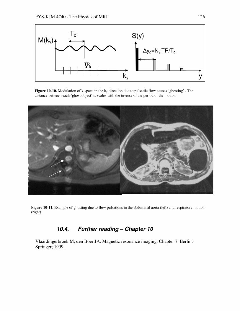
FYS-KJM 4740 - The Physics of MRI 126
10.4. Further reading – Chapter 10
Vlaardingerbroek M, den Boer JA. Magnetic resonance imaging. Chapter 7. Berlin: Springer; 1999.
ky
M(ky) Tc
∆yg=Ny.TR/Tc
S(y)
y
TR
Figure 10-10. Modulation of k-space in the ky-direction due to pulsatile flow causes ‘ghosting’ . The
distance between each ‘ghost object’ is scales with the inverse of the period of the motion.
Figure 10-11. Example of ghosting due to flow pulsations in the abdominal aorta (left) and respiratory motion (right).

FYS-KJM 4740 - The Physics of MRI 127
11. MR Contrast Agents In order for an excited spin system to return to its equilibrium magnetization, energy must be transferred from the spin system to the lattice (surrounding), as discussed in Chapter 1. The return to equilibrium is described by the spin-lattice relaxation time, T1. When T1-weighted sequences are used, the magnitude of the MR-signal increases with decreasing T1-relaxation times. Further, the contrast between two tissues will of course also increase with increasing difference in T1 relaxation times between the two tissues. However, the inherent difference in T1 relaxation time between biological tissues, or between normal and pathologic tissue is not always large enough to obtain a detectable contrast in the MR image. Sufficient contrast is of particular importance in differentiating pathological tissue from normal surrounding tissue. Exogenous MR contrast agents were therefore developed shortly after the first commercial MR systems became available in the early 1980’s. Today, MR contrast agents are typically in a significant proportion of MR examinations; with the highest usage in CNS applications (tumor diagnosis). MR contrast agents are also widely used in MR angiography (MRA). MR contrast agents act by selectively reducing T1 (and T2) relaxation times of tissue water through spin- interaction between electron spins of the metal-containing contrast agent and water protons in tissue and in the following sections we shall discuss in some details the mechanism of action of these agents and how it affects the MR signal intensity in vivo.
11.1. Classification of MR contrast agents
Although gadolinium based agents are by far are the most commonly used class of MR contrast agents to date, many other types of agents have started to appear on the market. The different classes of contrast agents can be classified according to 1) the magnetic property of the agent, 2) the dominant effect of the agent on the signal intensity and 3) the bio-distribution of the agent. Figure 11-1summarizes the different classes of agents according to these properties.
11.1.1. Magnetic properties
Paramagnetism
Most MR contrast agents in clinical use to date are based on the paramagnetic metal ions. Paramagnetic materials are metals with unpaired electrons in the outer orbital shells (transition and lanthanide metals), giving rise to magnetic dipoles when exposed to a magnetic field. Since the magnetic moment of an electron is about 700 times larger than that of a proton (due to smaller mass), the paramagnetic ions induce large fluctuating magnetic fields experienced by nearby protons. If the frequency of this fluctuation has a components close to the Larmor frequency it will result in a significant enhancement of proton relaxation. There are many paramagnetic metal ions that could potentially be used as MR contrast agents but the transition metal gadolinium (Gd3+) is by far the most commonly used. This is due to a favorable combination of many (seven) unpaired

FYS-KJM 4740 - The Physics of MRI 128
electrons combined with a long electron spin relaxation time which makes this metal a very efficient relaxation enhancing agent. The importance of a long electron spin relaxation time for efficient T1-relaxation will be discussed below.
Superparamagnetism Superparamagnetic agents are based on magnetite (Fe3O4) or maghemite (γ-Fe2O3) water insoluble iron oxide crystals with a core diameter in the range 5 – 10 nm. These crystals are often referred to as nanoparticles, and each nanoparticle contains several thousand paramagnetic Fe ions (Fe2+ and Fe3+). If the Fe ions are magnetically ordered within the crystal, the net magnetic moment of the nanoparticle is so large that it greatly exceeds that of typical paramagnetic ions. This effect is referred to as superparamagnetism and is characterized by a large magnetic moment in the presence of an external magnetic field but no remnant magnetic moment when the field is zero. Superparamagnetic agents can also induce strong enhancement of the T1- relaxation rate of water (depending on size and composition of the particles), but their dominant effect is on T2/T2* relaxation due to the large magnetic moment of the nanoparticles. Although superparamagnetic agents will not be specifically discussed in more detail here, the modes of relaxation enhancement observed with these agents are similar to the ones observed with gadolinium agents, but, as mentioned, with generally stronger effects on transverse relaxation.
Figure 11-1. Classification of MR contrast agents based on magnetic properties, biodistribution and dominant image enhamcenement

FYS-KJM 4740 - The Physics of MRI 129
11.1.2. Biodistribution
The biodistribution of a contrast agent describes how the agent is distributed in vivo after intravenous administration (all current agents are administered by i.v injection). ECF agents Small molecular weight (MW) paramagnetic agents are small enough to diffuse from the plasma into the interstitium and are thus distributed to the extracellular fluid. These agents are therefore often referred to as ECF agents. They are not taken up by cells and are therefore eliminated by renal excretion with a half-life determined by the glomerular filtration rate. Intravascular agents Intravascular agents are contrast agents with a MW large enough to prevent leakage from the vascular to the intravascular space. All iron oxide particles are intravascular agents, with a half-life in blood ranging from a few minutes to several hours. Iron oxides are eventually eliminated from the blood by phagocytosies and are thus taken up by the Kupffer cells of the liver, spleen and lymphatic system. In blood, iron oxide agents with the appropriate composition can produce significant T1-shortening – and several studies have investigated the use of nanoparticles for MR angiography. Once taken up by the liver the nanoparticles will be accumulated into larger particulate clusters in the Kupffer cells and relaxation will be completely dominated by T2/T2* effects. Iron oxides can thus be said to be both intravascular agents as well as tissue specific agents. Other types of intravascular agents exist which are based on macromolecular gadolinium compounds. Such agents are designed either by linking Gd3+ ions to a macromolecular polymer during synthesis or by making the Gd3+complex bind to plasma proteins after injection and thus forming macromolecules in blood Tissue specific agents Tissue specific agents are agents which have been specifically designed to accumulate in a given organ or tissue type. We have already seen that iron oxide nanoparticles are liver specific agents (as well as spleen and lymph node specific), and this class of agents have been shown to offer clinical utility in detecting liver lesions (by making normal liver parenchyma dark, rendering liver lesions hyperintense) after contrast agent accumulation in the liver. Other liver specific agents have also been developed, based either on Gd3+ or on the paramagnetic ion Mn2+. Contrast agents have also been developed, and are in clinical testing, for targeting of atherosclerotic plaques as well as different types of tumor antibodies.
11.1.3. Image enhancement
The effect of the contrast agent on the signal intensity can either be positive (increase in signal or T1-enhancement) or negative (signal reduction or T2-enhancement). As will be discussed in the next sections almost all MR contrast agents will affect both T1- and T2- relaxation times and the distinction between T1- and T2- enhancing agents is therefore somewhat artificial and will depend on many MR-specific parameters as well as contrast agent dose. In order to quantify the effect of the agent on signal intensity we need to

FYS-KJM 4740 - The Physics of MRI 130
quantify the relaxation enhancing capability of the particular agent in question. This issue will be dealt with the following sections
11.2. Contrast agent relaxivity
The ability of a contrast agent to enhance the proton relaxation rate is defined in terms of its relaxivity:
Eq. 11-1
H9, = 19, = H:9, + I9,J
where R0
1,2 are the relaxation rates (R1,R2) without the presence of the contrast agent, C is the (molar) concentration of the contrast agent and r1,2 are the relaxivity constants (T1- and T2-relaxivity) of the agent. The unit of r1 and r2 are mM-1s-1 (where mM = 10-3
mole/Litre). Note that Eq. 11-1assumes a linear relationship between contrast agent concentration and increase in relaxation rate. As will be shown later in the chapter, this is not always the case in tissues in vivo. Paramagnetic relaxation enhancement is commonly divided into inner-sphere and outer-
sphere effects. Inner-sphere effects induce both T1- and T2- relaxation and require a direct interaction (binding) between the paramagnetic centre and the water protons (at the hydration site of the paramagnetic ion). The proton T1- and T2-relaxivities due to inner sphere relaxation can be expressed as:
Eq. 11-2
I9 = F K9E + E
I = KE 3E+E9E9 + ∆ωLE9 + E9 + ∆ωL 4
where A is a constant, q is the number of coordinated water molecules per metal ion and τm is the residence time (chemical exchange) of the water molecules at the coordination site of the metal, T1m and T2m are the relaxation times of bound water and ∆ωm is the chemical shift difference between bound water and bulk water. T1m and T2m are complex functions of the properties of the contrast agent and depend strongly on the ability of the water protons to get in close proximity of the paramagnetic centre as well as on the rotational dynamics of the contrast agent molecule. The paramagnetic relaxation theory was originally derived by Solomon and Bloemenberg in the 1950’s and its details are way beyond the scope of this compendium. However, it should be mentioned that the contrast agent relaxivity is strongly dependent on the ‘effective’ correlation time which is given by:

FYS-KJM 4740 - The Physics of MRI 131
Eq. 11-3 1/N = 1/ + 1/O + 1/E where τr, τs and τm are the correlation times, respectively, of rotation (of the contrast agent molecule), electron spin relaxation (of the unpaired electrons) and chemical exchange (inverse of the lifetime of binding time of the water molecule to the paramagnetic ion). Proton relaxation due to paramagnetic interaction is related to the correlation times through spectral power density functions of the forms:
Eq. 11-4
N1 + PQN RS T1 + PUO
where ωI and ωS are the proton and electron Larmor frequencies, respectively. It therefore follows that effective relaxation requires that τc and τs are close to the proton and electron resonance frequencies, respectively. For a given correlation time the relaxivity of paramagnetic agents is thus dependent on field strength with decreasing relaxivity with increasing fields and in the high field limit r1 tend to zero whereas r2 approaches a value which is proportional to τc (derivation not shown here). τr is related to the size and molecular weight of the contrast agent, with larger molecules in general giving slower rotational correlation times. The electron spin relaxation time, τs, is an intrinsic property of the paramagnetic ion, and for gadolinium is of the order of 10-8 seconds which is ‘long’ enough to avoid that the overall correlation time 1/ τc is dominated by τs (making τc too short for effective relaxation to take place). Other paramagnetic ions, like dysprosium (Dy3+) exhibit very low T1-relaxivity in spite of seven unpaired electrons due to a very short electron spin relaxation time (10-13 sec). In addition to the importance of optimal correlation time τc, we observe that the contrast agent relaxivity is directly proportional to the number of water molecules (q) directly coordinated to the paramagnetic ion. In the Gd3+ aqua ion there are eight inner-sphere water molecules, resulting in a high relaxivity. However, the Gd3+ ion itself is rather toxic and needs to be incorporated in a ligand to prevent the Gd3+ ion to interact with endogenously available anions. The ligand is a biocompatible molecule which binds strongly to the paramagnetic ion to form a stable metal chelate. Many different gadolinium chelates are available for clinical use today; most of which are small molecular weight agents with a molecular weight (MW) of the complete chelate of less than 1000 daltons. Figure 11-2 shows the configuration of one commercially available gadolinium chelate (GdDTPA-BMA, OmniscanR). We see that a the gadolinium ion is

FYS-KJM 4740 - The Physics of MRI 132
surrounded – and tightly bound- to a ligand which occupy seven of the eight available bindings sites of the gadolinium – leaving a single binding site available for water. The effective T1-relaxivity (r1) of this (and many similar) gadolinium chelate is about 4 mM-1s-1 (at 20 MHz) and the T2-relaxivity is slightly higher. It should be stressed that the relaxivity of MR contrast agents is usually measured in water (at specified field strength and temperature) and the effective in vivo relaxivities may differ significantly from the in vitro values, as discussed in later sections.
11.3. In vivo relaxivity and MR contrast enhancement
We have seen in the previous section that the efficiency of a contrast agent to enhance the relaxation rates 1/T1 and 1/T2 is defined in terms of the relaxivities (r1,r2) of the agent. We shall now discuss in more detail the effect of relaxation enhancing agents on the MR signal intensity. In addition to the ‘dipolar’ relaxation effects discussed above, there is an additional contrast agent relaxation effect due to local variations in the Larmor frequency induced by the magnetic moment of the contrast agent. This is commonly referred to as ‘susceptibility induced relaxation’ and will be discussed in more details below. But first we will discuss the effects of dipolar relaxation resulting from a direct interaction between water protons and the paramagnetic centre.
11.3.1. Dipolar relaxation
It should initially be mentioned that, unlike e.g. in CT, the ‘dose response’ due to MR contrast agents in general highly non-linear. This means that the effect of the agent (on
Figure 11-2. Example of a gadolinium chelate (GdDTPA-BMA) formed by covalent binding of the gadolinium ion the a biocompatible ligand

FYS-KJM 4740 - The Physics of MRI 133
the measured MR signal intensity in a given sequence) is not linearly related to the contrast agent concentration in a given voxel. This may not be a major problem if we are only interested in a qualitative assessment of contrast agent enhancement, but it is a major problem if we need to relate the change in signal intensity to absolute (or even relative) concentration. From the expressions for contrast agent induced change in relaxation rates, given in Eq. 11-1 the corresponding changes is MR signal intensity can readily be estimated for a given pulse sequence given that the relaxivity values (r1,r2) of the agent are known. Assuming a SE sequence, the SI change due to the contrast agent is thus given by:
Eq. 11-5 VJ = W1 − exp −H:9 + I9JHexp −H: + IJX
where r1, r2 are the T1- and T2- relaxivities, respectively, for the agent, C is the contrast agent concentration and R0
1, R0
2 are the T1- and T2- relaxation rates, respectively, without the contrast agent. Figure 11-3 shows the change in SI as a function of CA concentration, assuming ρ=100, r1=4 mM-1s-1 and r2=4.5 mM-1s-1, R0
1=1 s-1 and R02=4 s-1, TR=500 ms
and TE=30 ms. As seen, the dose response is highly non-linear. However, within an initial concentration range, a fairly linear increase in SI is observed with increasing concentration. At higher concentrations, signal saturation occurs meaning that a further reduction in T1 does not result in a further increase in SI since the longitudinal magnetization is fully
recovered. Further, when the concentration becomes very high (depending on the TE) the signal will start to fall with further increase in C since the T2-effects of the contrast
0 1 2 3 4 530
40
50
60
70
80
CA concentration (mM)
Rel
SI
Figure 11-3. Simulated dose response of an MR contrast agent (CA) in a SE sequence. Initially T1-relaxation dominated but as the CA concentration becomes sufficiently high T1-saturation as well as counter-acting T2-relaxation becomes dominant resulting in signal reduction at higher concentrations

FYS-KJM 4740 - The Physics of MRI 134
agent will start to dominate the signal behavior. Figure 11-4 shows a sample of a patient with a brain tumor imaged with a SE sequence before (left) and after administration of a gadolinium based ECF-agent. Note the strong local T1-enhancement in the rim of the tumor. The contrast agent does not leak out from the intravascular space in normal brain tissue due to the presence of a blood-brain-barrier (BBB) which prevents even small MW molecules like Gd-chelates to enter the intenstitium. Since the intravascular volume in the brain is small (< 5%) little enhancement is thus seen in healthy brain tissue. In brain tumors, however, the BBB can often be disrupted due to various pathological processes, resulting in a selective accumulation in the extravascular space in the tumor, as seen in the figure. The fact that many pathological processes alter the permeability of the BBB, resulting in selective accumulation of the MR contrast agents is, in fact, the main reason why these agents are so useful for CNS imaging since the absence/presence of CA leakage as well as the pattern of contrast enhancement can give important indications as to the type of pathology present. Therefore MR contrast agents not only increase the sensitivity (the ability to detect) but also the specificity (the ability to differentiate) of the diagnostic procedure.
We observed in the simulation of Figure 11-3 that at high CA concentrations, the SI fell with further increase in CA concentration, even in a highly T1-weighted SE sequence. This can of course be a problem if, for some reason, the local CA concentration is so high that the signal has returned to baseline due to counter-acting T2-effects, thus giving the false impression of no contrast agent being present. In other situations, the T2-relaxivity of MR contrast agent is utilized specifically for different diagnostic purposes. This leads us on the topic of susceptibility induced relaxivity and will see that the T2-relaxivity of MR contrast agents in vivo in many situations, in fact is much higher than what is predicted by just the dipolar component discussed so far.
Figure 11-4. Example of the effect of a Gd3+-based ECF agent in a patient with a brain tumor. The contrast agent is selectively taken up in the tumor region due to pathological changes in the blood brain barrier (BBB) whereas an intact BBB prevents contrast agent accumulation in unaffected brain tissue.

FYS-KJM 4740 - The Physics of MRI 135
11.3.2. Water exchange effects
Dipolar relaxivity is dependent on direct interaction between water protons and the paramagnetic centre of the contrast agent. The linear relationship between relaxation rate and contrast agent concentration assumes that all protons which contribute to the MR signal have equal and unrestricted access to the paramagnetic ion on a time-scale equal to the T1 relaxation time of the medium. This condition is referred to as ‘fast exchange’ and the requirement for fast exchange can be expressed in terms of a correlation time, τ, so that:
Eq. 11-6 1 ≫ 1/9,9 − 1/9,
where 1/ τ is the rate of water exchange between the compartments with relaxation rates 1/T1,1 and 1/T1,2, respectively. In vivo, the two compartments can for instance be the intravascular and the extravascular (interstitial) compartment or the intra- and extracellular compartments of the extravascular space. The effect of limited water exchange on proton relaxation can be addressed by addition of a two-site water exchange terms to the Bloch equation describing the rate of magnetization between two compartments:
Eq. 11-7 59 = 5: − 599,9 − Z959 + Z5
5 = 5: − 59, − Z959 − Z5
where 1/T1,1, 1/T1,2 are the longitudinal relaxation rates of the two compartments, M0 is the equilibrium magnetization for the two compartments and k1, k2 are the water exchange rates between the two compartments. Figure 11-5 shows a schematics illustration of the water exchange process between the intravascular compartment (containing gadolinium) and the extracellular compartment. The exchange rate 1/τ introduced in Eq. 11-6 is the sum of the two rate constants k1+k2 so that 1/k1 (τ1) and 1/k2 (τ2) describe the average lifetime of the spins within the two compartments. The rate constants k1 and k2 are related (through mass balance) and k2 can be expressed in terms of k1 as follows:
Eq. 11-8
Z = Z9 [9\ − [9
where ξ1 is the relative volume of compartment 1 and λ is the ratio of proton spin densities in compartment 2 vs compartment 1.

FYS-KJM 4740 - The Physics of MRI 136
The general solution to Eq. 11-7 is described by a bi-exponential function of the form:
Eq. 11-9 5 = 5: + ]9 exp−^9 + ]exp −^ where c1,c2,u1,u2 are functions of k1,k2, 1/T1,1 and 1/T1,2. It can be shown that if the volume of compartment 1 is small or fast exchange conditions apply then Eq. 11-9 is well approximated by the well known mono-exponential relaxation curve following an inversion (180o) RF-pulse:
Eq. 11-10 5 = 5:1 − 2 exp−H9
Figure 11-5. Schematic illustration of water exchange between two tissue compartments; one containing contrast agent (intravascular space) and an extravascuclar space.
where R1 is now the ‘effective’ tissue relaxation rate of a two-compartment system and is given by:
Eq. 11-11
H9 ≈ ^ = 12 H9,9 + Z9 + H9, + Z − 12 `H9,9 + Z9 − H9, − Z + 4Z9Z

FYS-KJM 4740 - The Physics of MRI 137
The effective tissue relaxation rate in a two-compartment system is thus a highly non-linear function of the relaxation rates in the two tissue compartments and the rate of water exchange between them. Figure 11-6 shows sample curves of R1 in tissue (i.e. in an image voxel containing both compartments) vs R1 in blood for different exchange rates k1. The initial slope of the R1-curve describes the fast exchange limit (R1,1-R1,2 << k1) and scales with the blood volume of the intravascular compartment. In the opposite extreme of slow exchange limit (R1,1-R1,2 >> k1) the value of R1 becomes independent of R1 in blood and approaches asymptotically a maximum value given by: R1
max=R1,2+k2.
Exchange limitations are of particular importance in the brain because the contrast agent is usually confined to the intravascular compartment due to the blood brain barrier. The water exchange rate across the capillary membrane is of the order of 100 ms, and the achievable T1-enhancement in the brain (with no BBB leakage) is thus limited by the intravascular blood volume and the water exchange constant. The non-linear dose-response in terms of 1/T1 is again of particular importance when the contrast agent concentration needs to be estimated based on the MR signal response, as for instance is the case in MR perfusion imaging. Figure 11-7 summarizes the expected R1 dose response in different tissues as a function of tissue blood volume and exchange rates. Note that a linear response is expected in blood due to fast water exchange (<10 ms) between plasma and the intracellular compartment of the erythrocytes.
Figure 11-6. Simulations of the relationship between R1 in blood and measured effective R1 in tissue in a two-compartment system with different water exchange rates between the two compartments.

FYS-KJM 4740 - The Physics of MRI 138
Figure 11-7. Summary of expected R1 dose-response in vivo in a two compartment system (typically brain tissue) after contrast agent enhancement.
11.3.3. Susceptibility induced relaxation.
Magnetic susceptibility effects were discussed in Chapter 9.1 and we defined susceptibility as the proportionality constant between applied magnetic field and induced tissue magnetization: Mz=χH0 (H=Bo/µ0). We also mentioned in Chapter Susceptibility induced relaxation. that a similar relationship existed for paramagnetic agents. The general theory describing the relationship between induced magnetization M and applied magnetic field H0, valid at all fields, is expressed classically by the Langevin function:
Eq. 11-12
5 = bc ?]dℎ =f:cg:Zh > − = Zhf:cg:>C
where N is the number of paramagnetic atoms per unit volume, m is the magnetic moment per atom, kB is the Boltzmann’s constant and T is temperature in Kelvin. For values of µ0mH0/kBT <<1 (valid for field strengths below approx 50 T!) this leads to the approximation:

FYS-KJM 4740 - The Physics of MRI 139
Eq. 11-13
5 = bcf:g:3Zh = jg:
With
Eq. 11-14
j = bcf:3Zh
where Eq. 11-14 is known as the Curie law (compare to Eq. 1-3 for nuclear susceptibility). It can therefore be concluded that, for paramagnetic contrast agents, the induced magnetization is proportional to the applied magnetic field and the concentration of contrast agent in tissue (N) and the square of the magnetic moment of the paramagnetic ion. As discussed in Chapter 9, transverse relaxation will therefore be enhanced if the contrast agent is unevenly distributed in tissue so that local susceptibility differences occur. This is referred to as susceptibility induced relaxation and only affects T2/T2* and not T1-relaxation. In fact, a contrast agent is almost always unevenly distributed in vivo due to multiple intra- and extracellular compartments. Most existing MR contrast agents are ECF agents and thus distribute to the extracellular compartments (blood plasma and interstitium). This means that local susceptibility differences due to the contrast agent will occur both in blood and in the interstitium, giving rise to enhanced T2 and T2* relaxation. The susceptibility effect does not affect the longitudinal relaxation times in tissue because the size of the field perturbing compartments in vivo are so large that the T1-relaxivity has dispersed to zero at clinical fields. This is an important point because it reflects a fundamental property of the proton relaxation enhancing processes induced by contrast agents; a contrast agent can induce T2/T2* relaxation without affecting T1 if the combination of field strength, the magnetization due to the perturber (the magnetic agent) and the size of the perturbation is such that T1-relaxivity has dispersed to zero. Any reduction in T1 does, however, always cause a reduction in T2/T2* since T2-relaxation is caused by the same relaxation mechanisms which causes T1-relaxation – but includes an additional term which is independent of field fluctuations so that T2/T2* relaxation does not disperse to zero at any fields. Given that the contrast agent is unevenly distributed in tissue, the resulting variation in susceptibility ∆χ thus gives rise to a local variation in Larmor frequency ∆ω=γ∆χB0, with consequent loss of MR signal due to transverse relaxation. The resulting T2/T2* ‘relaxivity’ due to susceptibility effects is a complex function of many parameters; including sequence type (SE vs GRE), tissue structure, contrast agent properties and dose. One simplification is to assume that protons are ‘static’ in the TE-period; i.e. that the variation in frequency across the voxel due to ∆χ is much larger than the variation in frequency experienced by each proton due to proton diffusion. This is the so-called ‘static dephasing scheme’ and the resulting modulation of MR signal intensity due to ∆ω can then be expressed as:

FYS-KJM 4740 - The Physics of MRI 140
Eq. 11-15
X, P = : Pexp −PXP∞
∞
Note that in a static dephasing regime, no additional signal loss will occur in a SE sequence since the effect will be completely compensated for by the 180o pulse. In order to determine the corresponding T2* relaxivity (assuming GRE sequences) due to ∆χ, the frequency distribution within each voxel P(ω) must be known P(ω) can be determined e.g. by spectroscopic (Fourier) analysis of the free induction decay (FID) signal. The proton spectrum is then identified in terms of the linewidth and lineshape of the frequency response. The most commonly observed frequency distribution in vivo is a Lorentzian distribution of the form:
Eq. 11-16
P ∝ l mm + Pn
where σ2 is the variance of the frequency distribution so that the linewidth (in terms of FWHH) of the distribution is given by 2σ. Inserting the expression for P(ω) into Eq. 11-15 we then have:
Eq. 11-17
X, P = : l mm + Pn exp −PXP = :exp −∞
∞ mX
The effective T2-relaxation due to a Lorentzian field distribution is thus given by T2*=1/ σ and the increase in relaxation rate R2*=1/T2* is proportional to the linewidth of the frequency distribution. If we assume that σ is proportional to the increase in susceptibility due to the contrast agent (a plausible assumption) which again is proportional to the contrast agent concentration (number of paramagnetic molecules per unit tissue), then the change is signal intensity due to the agent in a T2/T2* weighted sequence (where T1-effects are assumed to be negligible) is given by:
Eq. 11-18 J = 0 exp−mJX = 0exp −ZJ ∙ X where C is the contrast agent concentration and k is a constant. The assumption of a Lorentzian lineshape in vivo may not hold in all tissues, and particularly in blood many studies have shown than the linehape is better approximated by a Gaussian function of the form:

FYS-KJM 4740 - The Physics of MRI 141
Eq. 11-19
P ∝ AB p−P2m q
The corresponding signal equation thus becomes:
Eq. 11-20
X, P = : AB p−P2m q exp −PXP = :exp ;−mX<∞
∞
We now see that the ‘effective’ relaxation rate is given by R2=σ2TE (so that =:exp −HX). The effective R2 is thus proportional to TE and to the square of contrast
agent concentration, C (assuming again that m ∝ J). Figure 11-9 shows sample spectra for a Gaussian (left) and Lorentzian lineshapes, both measured in blood. The Lorentzian lineshape is observed in fully oxygenated blood (no paramagnetic species) whereas the Gaussian lineshape is observed in deoxygenated blood due to the presence of paramagnetic deoxyhemoglobin or in oxygenated blood containing a paramagnetic contrast agent. Figure 11-8 summarizes the expected R2* dose response as a function of contrast agent concentration (relative units) in different tissues. Note the linear response in tissue (where the slope scales with tissue blood volume) due to a predominant Lorentzian lineshape whereas a quadratic relationship is expected in blood containing contrast agent where the field distribution is better described by a Gaussian function (Eq. 11-19).
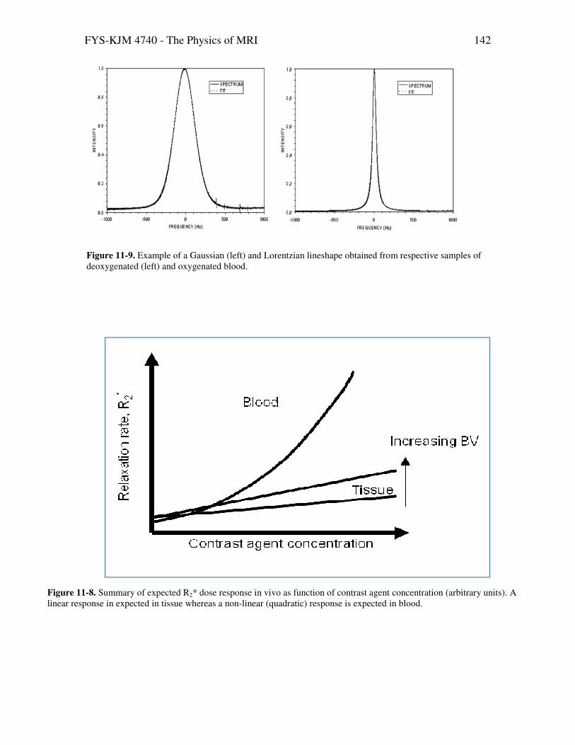
FYS-KJM 4740 - The Physics of MRI 142
Figure 11-9. Example of a Gaussian (left) and Lorentzian lineshape obtained from respective samples of deoxygenated (left) and oxygenated blood.
Figure 11-8. Summary of expected R2* dose response in vivo as function of contrast agent concentration (arbitrary units). A linear response in expected in tissue whereas a non-linear (quadratic) response is expected in blood.

FYS-KJM 4740 - The Physics of MRI 143
11.4. Further reading Chapter 11
1. Merbach and Tóth (eds). The Chemistry of Contrast Agents in Medical Magnetic
Resonance Imaging. John Wiley & Sons, Ltd. ISBN 0-471-60778-9. (2000). 2. Rocklage, Watson and Carvlin. Chapter 14 In Stark and Bradley (eds); Magnetic
Resonance Imaging (2nd edition). Mosey Year Book (1992). 3. Bjørnerud. Proton Relaxation Properties of a particulate Iron Oxide MR Contrast
Agent in Different Tissue Systems. PhD thesis. Uppsala 2002 (ISBN 91-554-5330-9).

FYS-KJM 4740 - The Physics of MRI 144
12. Advanced Applications of MR Contrast Agents As we have already seen in the previous chapter, MR contrast agents can be used to modify the MR signal intensity in many different ways, depending on tissue structure, contrast agent type and concentration as well as MR sequence parameters. The ‘classical’ application of MR contrast agents is based on static images where areas of increased contrast agent update secondary to pathology are detected. Such applications still account for the large majority of contrast enhanced MRI. However, there is an increasing use of dynamic analysis of contrast enhancement whereby tissue function can be more directly assessed. Since this is an important area (especially for MR physicist) some of these methods will be discussed in a separate chapter (this one). As we shall see later in the chapter, most dynamic imaging techniques require some sort of estimation of the contrast agent (CA) concentration (or at least relative concentration). We will therefore start by addressing how the CA concentration is related to the measured MR signal using different imaging techniques.
12.1. T1-based dynamic imaging
In T1-based perfusion imaging, the sequence is made optimally T1-sensitive and minimally T2/T2* sensitive. The most linear results are obtained if T1-relaxation times are measured directly (e.g. using a saturation recovery or inversion recovery sequence). The great advantage of measuring T1 is thus that transverse relaxation effects as well as signal saturation are completely eliminated. The change in T1 relaxation rate due to the contrast agent is then given by:
Eq. 12-1 ΔH9 = H9 − H9: = JsI9
where H9: is the T1 relaxation rate before contrast arrival and r1 is the T1-relaxivity of the contrast agent (see Eq. 11-1). Even if r1 is not known the concentration is still known to within a constant as long as we can assume the relaxivity of the agent to be the same in all tissues of interest and that fast water exchange can be assumed between all sub-compartments within each image voxel. The main disadvantage is that it takes time to measure T1-relaxation times and temporal resolution therefore needs to be scarified. An alternative to estimating T1 at each time-point is to acquire images with an extremely T1-weighted GRE sequence. As long as TR<< T1 and TE<<T2* and the flip angle is large the
signal response can then be approximated to V ∝ tuvw (see spoiled GRE equation in
Chapter 4.2). We thus have an approximately linear dose response as long as 1/T1 is proportional to contrast agent concentration (e.g. fast exchange condition described in Chapter 11).

FYS-KJM 4740 - The Physics of MRI 145
12.2. T2/T2* based dynamic imaging
T2- or T2* weighted dynamic imaging is also often referred to as dynamic susceptibility contrast (DSC) imaging. DSC imaging is particularly useful in the brain. Because small MW Gd-agents are effectively intravascular agents in the brain (due to the BBB) the volume of distribution is limited by the cerebral blood volume (less than 5% in the brain). T1-enahncement, being limited by intra- extravascular water exchange is therefore limited in the brain. The susceptibility effect, on the other hand, is a long range effect and will affect protons far outside the intravascular compartment – thereby giving a much larger dynamic signal change compared to the T1-effect. Most DSC sequences are EPI based (either SE-EPI or GRE-EPI). In both cases we can express the dynamic signal response as:
Eq. 12-2 V = V0x5:, 9exp −X ∙ ΔH where SI(0) is the signal intensity at baseline (prior to contrast arrival f(T1) is some function of M0 and T1, TE is the echo time and ∆R2 (t) is the change in transverse relaxation rate (1/T2 for SE- or 1/T2* for GRE- based EPI) due to the contrast agent. If we assume T1-effects to be negligible, we then have
Eq. 12-3
ΔH = Z ln pVV0q /X ∝ J
Where C(t) is the dynamic contrast agent concentration. We here assume a mono-
time
Raw data
∆R2* maps
t=0
Figure 12-1. Dynamic T2* weighted imaging following a bolus injection of a gadolinium based ECF agent. The top row shows the raw data and the bottom row the R2*-converted images using Eq. 12-3. The contrast agent was injected at t=0. Note the negative (T2*) effect of the contrast agent in the raw images whereas the effect is positive and scales with CA concentration in the R2* images.

FYS-KJM 4740 - The Physics of MRI 146
exponential relationship between ΔH and SI and a linear relationship between ΔH and C (in other words a Lorentzian lineshape as discussed in previous chapter). Figure 12-1
shows an example of DCS images before and after conversion to ΔH. The dynamic series of ΔH maps are used for further analysis of different perfusion related parameters as will be discussed in the next section.
12.3. Perfusion imaging
Perfusion imaging is a collective term used here to describe different contrast enhanced methods for assessing tissue perfusion (or perfusion related parameters). These methods are based on the simple concept that, since the contrast agent is distributed (initially) in the blood, then the temporal effect of the agent on the signal intensity in a given body region (or tissue) must somehow be related to the function of the tissue (in terms of blood perfusion or possibly tissue blood volume). So, if the contrast agent is administered as a rapid bolus injection and the effect e.g. in the brain is monitored with sufficient temporal resolution, the resulting dynamic curve (depicting change in MR signal intensity vs time) should contain relevant functional information. The theory of deriving functional information from the observed effect of a ‘tracer’ (in our case the MR contrast agent) is historically referred to as tracer kinetic modeling and much of the theoretical foundation for these methods were developed already in the 1950’s. A central concept to all perfusion imaging is the so-called central volume
principle stating that the volume of a given tissue is equal to the blood flow into the tissue multiplied by the mean transit time of the tracer through the tissue. The tracer kinetic models further assume that the contrast agent is distributed in the intravascular (plasma) space only. This is true for all contrast agents in the central nervous system (when the BBB is intact) but only true for large MW intravascular agents outside the CNS. With reference to Figure 12-2, the central volume principle can be expressed as:
Eq. 12-4
zs = ∙ 5 = K: Js|:
Where q0 is the amount of contrast agent (mmol) injected. The integral is practice taken from the time of contrast arrival (t=0) to the exit of the first passage of the contrast bolus.

FYS-KJM 4740 - The Physics of MRI 147
We note that, in order to estimate tissue blood volume we need know the concentration time curve of the contrast agent as well as the flow into the tissue of interest. We shall come back to the estimation of flow, but for the time being we assume that Fa is a constant (e.g. the total flow into the brain) so that we can at least compare different regions of tissue (e.g. different brain regions) supplied by the same arteries. A second requirement is that Ct(t) can be measured, and we discussed in the previous sections how we at least can obtain relative measured of C(t) for both T1- and T2/T2* weighted images (with certain assumptions). If, in addition to Ct(t) we are also able to measure Ca(t), i.e the arterial input function (AIF) we can obtain a better estimate of Vt by normalizing the tissue response to the AIF:
Eq. 12-5
zs = Z Js|: J|: ∝ ∆Hs ∆H
where ∆R2t and ∆R2a are the change in R2 (or R2*) in the tissue of interest and the artery supplying the tissue, respectively.
MR based blood volume (BV) imaging has proved to have great utility in the diagnosis of brain tumors (gliomas). High grade (malignant) gliomas tend to have BV than low grade gliomas, probably due to higher angiogenetic activity (large formation of tumor specific blood vessels). Many studies have shown that BV maps generated from dynamic MRI can provide much better differentiation between high- and low grade gliomas than conventional contrast enhanced MRI.
Figure 12-2. The concept of the central volume principle, relating tissue volume to flow.
Fa
Vt
MTT
Ct(t)Ca(t)

FYS-KJM 4740 - The Physics of MRI 148
Figure 12-3. Generation of blood volume maps from DSC data. The raw data is first converted to ∆R2* maps and relative BV is then calculated on a pixel-by-pixel basis from the area under the ∆R2* vs time curve.
Figure 12-3 shows the process of generating relative BV maps from raw DSC data. Here DSC images were acquired using a GRE-EPI sequence with a temporal resolution of about 1.5 seconds.
Figure 12-4 shows image from a patient with a high grade glioma. The BV map clearly shows a distinct region of elevated BV values (circle in the right image) corresponding to the most malignant part of the tumor. These so-called ‘hot spots’ have been shown to be a much more specific marker for tumor grade than conventional contrast enhanced MRI.
∫∆∝ dttRrCBV )(2
−=⋅=∆
0
*
2
)(log)()(
SI
tSI
TE
ktCktR e
Figure 12-4. DSC imaging in a patient with a high grade glioma. The tumor (including aedema) is clearly visible on T2-weighted image (left) with strong contrast enhancement evident on T1-w image after gadolinium administration (centre). The corresponding BV map shows a distinct area of high blood volume in one region of the tumor which corresponds to the most malignant area of the tumor.

FYS-KJM 4740 - The Physics of MRI 149
So far we have discussed how to estimated tissue blood volume, but in some circumstances (e.g. in the diagnosis of tissue ischemia or stroke) tissue perfusion is a more clinically important parameter. Tissue perfusion, Ft, is defined as blood flow per unit volume of tissue (mL/sec/100 g tissue) and it can be shown that Ft is related to Ct(t) as follows:
Eq. 12-6
Js = s H − J = sH ⊗ J s:
where R(t) is the residue function and describes the theoretical tissue impulse response which reflects the true dispersion of the contrast bolus (or the tissue response following a delta input function). We have that R(0)=1 since, by definition, no contrast agent has yet left the tissue at t=0. Eq. 12-6 describes a standard convolution integral and Ft can be determined by deconvolution of the measured concentration time curves (or, more precisely, corresponding in ∆R1 or ∆R2) in the artery and tissue. There are many standard mathematical approaches that can be used to solve deconvolution integrals of this form, but one of the most common techniques is singular value decomposition (SVD). When Ft and Vt have been determined, the mean transit time can be estimated according to the central volume principle:
Eq. 12-7
5 = zss
MTT is related to the ‘mismatch’ between perfusion and blood volume and this parameter has proved to be particularly important is cerebral stroke assessment. Figure 12-5 shows a sample case from a patient with acute stroke. The area of elevated MTT
BV BF MTT
Figure 12-5. DSC perfusion images in a patient with acute stroke. Note the elevated MTT values in the affected region (circle) representing tissue at risk of infarction due to mismatch between blood volume and blood flow (stagnant blood)

FYS-KJM 4740 - The Physics of MRI 150
values in the right image (circle) represent tissue at risk of infarction due to severely reduced flow.
12.4. Dynamic contrast enhanced imaging
Dynamic contrast enhanced (DCE) MR imaging is a collective term used to describe different methods assessing the dynamic effect of an MR contrast agent following a rapid bolus injection. DCE imaging usually referrers to dynamic imaging outside the central nervous system (i.e. not including brain perfusion imaging as discussed in the previous section). As discussed in the Contrast Agent chapter, small MW contrast agents are only intravascular agents in the CNS and will leak into the interstitial space in all other body areas. The rate at which the contrast agent diffuses from plasma to the interstitium (and eventually back to plasma) is determined both by physiological parameters (blood flow and the permeability or ‘leakiness’ of the capillary wall) as well as properties of the contrast agent (e.g. molecular size, configuration and charge).Since most DCE imaging today is performed using conventional gadolinium based extracellular fluid (ECF) agents, we will restrict the discussion to such agents. The mathematics describing the dynamic distribution of the contrast agent in vivo is referred to as kinetic modeling and for Gd-ECF agents the distribution is for most situations well described by a two-compartment model as illustrated in Figure 12-6. In a two-compartment model, the contrast agent is assumed to reside either in the plasma space or in the extravascular, extracellular space
(EES) and the flux of contrast between the two compartments is described by two transfer constants. Mathematically, this dynamic system can be described by the following differential equation:
Ktrans
kep
EESPlasma
Figure 12-6. Two-compartment representation of contrast leakage from the intravascular space to the extravascular, extracellular space (EES). The flux of contrast agent between the two compartments are described by the two tranfer-constants Ktrans and Kep.

FYS-KJM 4740 - The Physics of MRI 151
Eq. 12-8 Js = s7OJ − ZTJs
where Ktrans and kep are the transfer constants as defined in Figure 12-6 and Cp and Ct are the contrast agent concentrations in plasma and EES, respectively. Assuming that the initial condition is zero it can easily be shown that the solution to Eq. 12-8 is given by the following convolution integral:
Eq. 12-9
Js = s7O J exp;−ZT − < s:
We see that, as was the case for perfusion analysis, we assume that the contrast agent concentration can be determined both in an artery (Cp) and in tissue (Ct) from the measured dynamic MR signal response. If both arterial and tissue contrast agent concentrations can be estimated (based on the assumptions described earlier) then the transfer constants can be determined using standard deconvolution mathematics. However, the plasma concentration (arterial input function) is often difficult to assess due to lack of arterial vessels in the image plane or too poor spatial resolution. In this case we can assume that the plasma concentration follows a certain time-course. If the temporal resolution is low, then Cp can be fairly well approximated by a mono-exponential function with a half-life equal to the elimination half-life of the contrast agent (around 60 minutes for renally excreted Gd-ECF agents). For higher temporal resolutions (seconds rather than minutes) Cp needs to be modeled by a bi-exponential function in order to include the initial distribution phase as well. If we model the plasma concentration as Cp=Cp(0)exp(-t/T1/2) (plasma half-life = T1/2) we then get:
Eq. 12-10
Js = s7OJ,:exp − 9 − ZTJs
This is a non-homogeneous equation (y’ + p(x)y=r(x)) with solution:
Eq. 12-11
Js = s7OJ,:9/ − ZT AB−ZT − AB p −9/q

FYS-KJM 4740 - The Physics of MRI 152
If we now assume that both Cp,0 and T1/2 are constants then Ktrans and kep can be determined using standard non-linear least squares curve fitting methods from the dynamic time-course of the contrast enhancement. Why do we want to determine the transfer constants Ktrans and kep ? Because these parameters may provide important information about the ‘leakiness’ of the capillary walls, which can be altered in many pathological conditions. A sample DCE case in a patient with arthritis is shown in Figure 12-7 (see figure caption for details). Areas of increased Ktrans i.e. increased ‘leakiness’ to the contrast agent are clearly seen as hot-spots in the parametric Ktrans color map.The increase in Ktrans is here probably due to inflammatory processes in the tissue caused by the arthritis. Many tumor types have also been shown to exhibit enhanced Ktrans value due to increased leakiness of tumor vessels formed by angiogenesis.
-10
0
10
20
30
40
50
60
70
80
0 20 40 60 80 100 120
Figure 12-7. DCE imaging in a patient with arthritis. The top image shows one of the raw T1-weighted images in the dynamic acquisition and the curves show the dynamic evolution of the contrast enhancement (in percent enhancement rel to baseline) from the two regions of interest. The color image shows the corresponding Ktrans image calculated from the dynamic curves using Eq. 12-11. Areas of increased ‘leakiness’ due to inflammatory processes are clearly seen as hot-spots in the image.

FYS-KJM 4740 - The Physics of MRI 153
13. MR Angiography As should be evident from the previous chapter, MRI is inherently sensitive to
flow, and this sensitivity can be used to selectively visualize flowing blood and hence the vascular system. These methods are collectively referred to as MR Angiography (MRA). There are three distinct and very different methods available in MRI for visualizing blood and these methods will be discussed separately.
13.1. Time-of-flight (TOF) MRA.
TOF MRA is based on the idea that blood flowing into an excitation volume (a slice) experiences fewer excitation pulses than the stationary tissue inside the slice. If a GRE sequence is used, we have seen in previous sections that the transverse magnetization is reduced with number of excitation pulses until a steady-state level is reached (Figure 4-8). If blood flow is fast enough so that the protons in blood only experience a single excitation pulse (on average) then the magnetization in blood vs tissue in steady state spoiled GRE sequence is given by:
Eq. 13-1
1
10max
)cos(1
))cos(1)(sin())(sin(
E
EMxyMM GRE
α
ααα
−
−=−=∆
where MxyGRE is the steady-state magnetization equation for spoiled GRE sequences (Eq. 4-8) and E1 = exp(-TR/T1). For a given TR/T1, the contrast increases with increasing flip angle (see Figure 13-2 ). In Eq. 13-1 we have assumed that M0 is the same in tissue and blood and that blood only experience a single excitation pulse. This means that the flow velocity, v, must meet the following criterion: v ≥ d/TR where TR is the repetition time and d is the slice thickness (Figure 13-1). If the velocity is less than d/TR then the blood signal will be a function of position within the slice. Further, if the vessel is not perpendicular to the slice, increasing signal saturation will occur in blood as the spins experience increasing number of excitation pulses after entering the slice. This gradual signal saturation, and consequent diminished blood signal, can give a false impression of vessel occlusion (Figure 13-7). If the blood experiences multiple excitation pulses then optimal flip angle becomes a function of TR/T1 and number of excitation pulses experiences by the flowing spins.

FYS-KJM 4740 - The Physics of MRI 154
d
v
Figure 13-1. The time-of-flight (TOF) concept. Blood flowing perpendicular to the slice direction (arrow) leads to constant inflow of non-saturated spins into the image slice, giving higher signal from blood
Figure 13-2. Examples of TOF effects in a 2D-GRE sequence in an axial slice thought the neck. Note the much higher blood-background contrast in the right image (flip angle = 60 deg) compare to in the left image (flip angle = 10 deg). TR=7.5 ms in both images.
α = 10o α = 60o

FYS-KJM 4740 - The Physics of MRI 155
# of RF pulses
Mxy
∆Mmax
Figure 13-3. Maximum contrast between inflowing blood (dotted line) experiencing a single excitation pulse in the imaged slice and the stationary background tissue (solid
line) in a spoiled GRE sequence.

FYS-KJM 4740 - The Physics of MRI 156
13.2. Maximum Intensity Projection (MIP)
The information in TOF images is usually visualized by creating so-called Maximum Intensity Projections (MIP). A MIP is a type of post-processing method whereby the brightest pixel intensity along multiple trajectories through the imaged volume is visualized as a 2D projection (Figure 13-4) By varying the angle of these
trajectories, 2D angiographic projections can be created from any chosen direction through the volume.
13.3. 3D-TOF techniques
One major disadvantage of 2D-TOF is the limited resolution in the slice-direction achievable in a 2D sequence. As seen in Figure 13-5, the limited slice-thickness in 2D-TOF sequences results in MIP images of limited diagnostic quality for other than assessing gross vascular anatomy. In order to increase the resolution in TOF sequences 3D-acquisitions must be used. We have seen in previous chapter that the much thinner slices can be acquired in 3D GRE sequences compared to 2D sequences. The disadvantage of 3D-TOF techniques vs 2D-TOF is increased scan-time. However, modern scanners can acquire high quality 3D TOF images with a sub-millimeter isotropic resolution in less than five minutes.
Figure 13-4. The concept of Maximum Intensity Projection (MIP) from multiple 2D TOF images
MIP

FYS-KJM 4740 - The Physics of MRI
Figure 13-6 shows the MIP from a angle =25 deg). Note the much higher spatial resolution compared to the 2DTOF, the image volume is usually divided into multiple 3D slabs which are excited separately in order to reduce signal satgradually increased as the flowing spins have experienced an increasing number of excitation pulses within each 3D slab. This variable flip angle approach tends to minimize blood saturation and hence increase thtissue in 3D TOF acquisitions.
Figure 13-5. The creation of a MIP from multresolution in the slice-direction causing ‘step’ patterns in the resulting MIP.
Figure 13-6. TOF, much higher resolution can be obtained in 3D
The Physics of MRI
the MIP from a 3D-GRE images obtained in the brain (TR=35 ms, flip Note the much higher spatial resolution compared to the 2D-
TOF, the image volume is usually divided into multiple 3D slabs which are excited separately in order to reduce signal saturation. Further, the flip angle is commonly gradually increased as the flowing spins have experienced an increasing number of excitation pulses within each 3D slab. This variable flip angle approach tends to minimize blood saturation and hence increase the contrast between blood and stationary tissue in 3D TOF acquisitions.
The creation of a MIP from multiple 2D TOF slices. Note the poor direction causing ‘step’ patterns in the resulting MIP.
MIP from a 3D TOF acquisition in the brain. Compared to 2D
TOF, much higher resolution can be obtained in 3D-sequences.
157
RE images obtained in the brain (TR=35 ms, flip -MIP. In 3D
TOF, the image volume is usually divided into multiple 3D slabs which are excited uration. Further, the flip angle is commonly
gradually increased as the flowing spins have experienced an increasing number of excitation pulses within each 3D slab. This variable flip angle approach tends to
e contrast between blood and stationary
MIP from a 3D TOF acquisition in the brain. Compared to 2D-

FYS-KJM 4740 - The Physics of MRI 158
13.4. Artery / vein selection – use of saturation slabs.
Since arteries and veins usually arrive a given slice from different directions, is is possible to selectively saturate the arterial or venous signal by applying so-called ‘saturation slabs’. These are regions place outside the image slice where multiple intense RF-excitation pulses are applied just prior to the TOF image acquisition (see Figure 13-8).
Figure 13-7. Signal saturation due to in-plane flow causes artificial loss of blood signal (arrows) which can be mistaken for vessel occlusions (absence of blood flow).
’sat.slab’’sat.slab’
Figure 13-8. Application of ‘saturation slab’ to selectively remove blood signal from veins returning from the brain in a neck TOF angio. Note that
arterial blood arriving from below are unaffected by the rest slab.
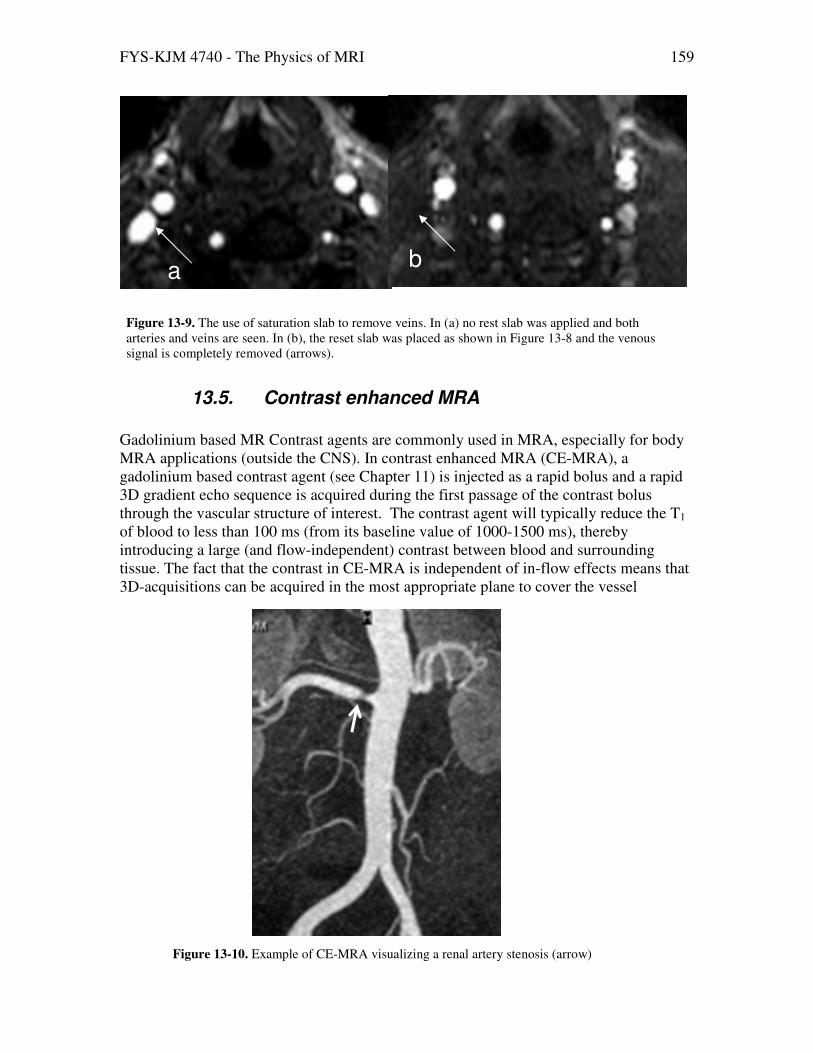
FYS-KJM 4740 - The Physics of MRI 159
13.5. Contrast enhanced MRA
Gadolinium based MR Contrast agents are commonly used in MRA, especially for body MRA applications (outside the CNS). In contrast enhanced MRA (CE-MRA), a gadolinium based contrast agent (see Chapter 11) is injected as a rapid bolus and a rapid 3D gradient echo sequence is acquired during the first passage of the contrast bolus through the vascular structure of interest. The contrast agent will typically reduce the T1 of blood to less than 100 ms (from its baseline value of 1000-1500 ms), thereby introducing a large (and flow-independent) contrast between blood and surrounding tissue. The fact that the contrast in CE-MRA is independent of in-flow effects means that 3D-acquisitions can be acquired in the most appropriate plane to cover the vessel
Figure 13-9. The use of saturation slab to remove veins. In (a) no rest slab was applied and both arteries and veins are seen. In (b), the reset slab was placed as shown in Figure 13-8 and the venous signal is completely removed (arrows).
ab
ab
Figure 13-10. Example of CE-MRA visualizing a renal artery stenosis (arrow)

FYS-KJM 4740 - The Physics of MRI 160
anatomy of interest. CE-MRA is the standard MRA method for assessment of e.g. renal stensosis and for the vessels of the lower extremities. Modern MR systems also enable ‘whole body’ MRA to be performed by moving the MR table in synchrony with the bolus passage through the body. CE-MRA requires accurate timing of the acquisition relative to the passage of the bolus through the arterial tree. If the images are acquired too early, little vessel enhancement is obtained whereas if the acquisition takes place too late, venous enhancement will occur, obscuring the visualization of the arterial vessels.
13.6. Further reading – Chapter 13
Current MR Angiographic Imaging Techniques, A Survey. Kouwenhoven M et al. Vascular Diagnostics. Springer-Verlag, Heidelberg (1994).

FYS-KJM 4740 - The Physics of MRI 161
14. Imaging Water Diffusion Diffusion refers to the random (Brownian) motion of molecules in a fluid (or gas). MRI can be used to probe water diffusion at a cellular level in vivo - both in terms of absolute rate of diffusion (diffusivity) and primary diffusion direction (anisotropy). Since both diffusivity and degree of anisotropy has been shown to be altered in many pathological processes, the ability of MRI to measure these tissue properties has proved to be of great importance both in clinical diagnostic routine as well as in basic neuro-science research. We have seen from the discussion in the previous chapter that the MRI is inherently sensitive to moving spins since they have a different effect on the MR signal relative to stationary spins. This motion sensitivity is taken one step further in diffusion MRI by making the MR signal sensitive to motion occurring on scale orders of magnitude smaller than the resolution of the MR image. Before we start the description of how MRI is sensitized to diffusion, a short summary of the concept of molecular diffusion is warranted.
14.1. Molecular diffusion
The concept of molecular diffusion was formalized by Albert Einstein in 1905, when he observed that the fundamental particle property was not its velocity but its mean displacement in a given time <r2(t)>. Einstein showed that the mean displacement (in 3D) of a particle with no diffusion restrictions (free diffusion) is given by:
Eq. 14-1 < I >= 6 where t is time and D is the diffusivity (m2/s, or more commonly mm2/s on a physiological scale) which is given by:
Eq. 14-2
= Z6H
where kb is Boltzmann’s constant, T is absolute temperature, η is the viscosity and R is the particle radius. The water diffusivity of human tissue is of the order of 3 x 10⁻⁹ m2/s. This means that the typical water diffusion length within the time window of an MR acquisition (echo time of 50 ms) is of the order of √<r2>≈30 um, as shown in Figure 14-1.

FYS-KJM 4740 - The Physics of MRI 162
Figure 14-1. Simulation of free diffusion (random walk) of a single particle diffusing for 50 ms with D=3x10⁻⁹ m2/s.
The molecular dynamics of a system of molecules with diffusivity D is described by Fick’s second law:
Eq. 14-3 Ф = ∇D
Where Ф is the particle concentration per unit volume (mol/liter), D is the diffusivity (m2/s) and t is time. In the one-dimensional case it can be shown that a solution to Eq. 14-3 is given by a Gaussian distribution:
Eq. 14-4
D, ∝ 1√ exp p−4q
When relating water diffusion to MRI signal, it is more relevant to think of diffusion in terms of probability P(x,t) of a given displacement x in time t. It can be shown that the probability distribution is equivalent to the concentration distribution and in the case of unrestricted diffusion is then given by:
Eq. 14-5
, ∝ 1√ exp p−4q
-8 -6 -4 -2 0 2 4 6 8 10 12
x 10-6
-14
-12
-10
-8
-6
-4
-2
0
2x 10
-6

FYS-KJM 4740 - The Physics of MRI 163
14.2. Diffusion weighted imaging
We have seen in the previous chapters that proton motion induces phase shifts in the MR signal. So far, we have only discussed the effect of bulk motion and we have seen that the effect of such motion can be compensated for by introducing additional gradients. Motion due to molecular diffusion is different because it is (by definition) completely random and any given image voxel will contain a very large number of diffusion trajectories. Intuitively, we may guess that water diffusion will introduce signal loss due to intra-voxel phase dispersion. We can formalize this diffusion induced signal attenuation by including a diffusion term in the Bloch equation introduced in Chapter 1. Since water diffusion only affects the transverse magnetization, we only consider the transverse component of M: MT=Mx + jMy which, including a diffusion term is given by:
Eq. 14-6 ts = − t − ∙ I5 + ∇5
(Compare this equation to the transverse component of Eq. 2-5) From Eq. 14-6 we observe that the diffusion term of Bloch’s equation is identical to the probability distribution given by Fick’s second law (Eq. 14-3). Although beyond the scope of this compendium, it can then be shown that (neglecting T2-relaxation and assuming constant gradient G applied during time τ) the solution to Eq. 14-6 in terms of the probability distribution P is given by:
Eq. 14-7
5, = 5, 0, AB− ∙
Introducing the ‘reciprocal space’ q= (in units of m-1, equivalent to the k-factor introduced in Chapter 2, Eq. 2-20) the transverse magnetization can then be expressed in term of the wave number, q:
Eq. 14-8 5 = WI, AB−K ∙
Here we have replaced the initial magnetization MT(r,0) with the proton density WI. We now see that the transverse magnetization is given by the Fourier transform of the diffusion induced displacement probability function P. In order to introduce diffusion sensitivity into an MR sequence a bipolar gradient pair is used so that the net effect of the gradients is zero for stationary spins. A sequence containing such a diffusion sensitizing gradient pair is called a Stejskal-Tanner sequence. The sequence layout is shown in Figure 14-2.

FYS-KJM 4740 - The Physics of MRI 164
Figure 14-2. The Stejskal-Tanner diffusion weighted sequence. The gradient pair induces a signal loss which scales with degree of diffusivity.
Let’s consider a spin at position r. The first gradient pulse will induce a phase shift of γδG.
r. Because of the 180o refocusing pulse, the second diffusion gradient will induce a negative phase shift of -γδG.
r’ where r’ is the position of the spin at the time of the second gradient pulse. The net phase effect due to the gradient pair is therefore Ф= γδG.(
r-r’) = γδG.R. It should be noted that such diffusion sensitization can be added to any sequence; in the case of the gradient echo readout, however, the second diffusion gradient must be of opposite polarity to the first since no RF refocusing is applied. Almost all current diffusion weighted imaging is based on SE-EPI sequences (usually single shot EPI, see Chapter 6.2). In the above sequence diagram, the spin echo would then be read out during an EPI echo train. In the following we assume that the diffusion gradient duration is much smaller than the diffusion time; i.e. δ << ∆. If this is not the case, it can be shown that the diffusion time must be replaced by an effective diffusion
time given by: ∆’= ∆- δ/3. It is also assumed that the diffusion gradients have ‘zero’ rise time (perfect square pulses). Substituting the diffusion time t=∆ and r=R in Eq. 14-8 and normalizing the proton density to unity (i.e MT=1 when G=0) we can thus express the magnetization in terms of the diffusion weighted parameters δ, G and ∆ :
Eq. 14-9 5 = , AB−K ∙
where q= δ. In the case of free diffusion, P is Gaussian as defined in Eq. 14-5 and we thus have:
Eq. 14-10
5 = 1√ exp p−H4q AB−K ∙

FYS-KJM 4740 - The Physics of MRI 165
This is the Fourier transform of a Gaussian distribution, and the result is therefore also a Gaussian and is given by:
Eq. 14-11 5 = exp−K2∆
Substituting q= δ and substituting transverse magnetization with relative signal we then have:
Eq. 14-12 = S0exp−2δ2∆ = S0exp −
The term 2δ∆ is commonly referred to as the ‘b-factor’ (units s/m2) and determines the amount of diffusion weighting in the sequence: a high b-factor gives high diffusion weighting. We therefore conclude that, in the case of free diffusion, the transverse magnetization (and hence MR signal) decays mono-exponentially with increasing diffusivity, D and diffusion weighting as given by the b-factor. It is now straight forward to generate a ‘mean diffusivity map’ from images with different degrees of diffusion weighting. With two b-values the diffusivity is simply given by:
Eq. 14-13
= − 1 − 9 dT =9>
Where S(b1) and S(b2) are the signal intensities with b-values b1 and b2, respectively (b2>b1).
Figure 14-3. Example of diffusion weighted images in a patient with acute stroke. The first three images (left-right) shows the effect of increasing diffusion weighting (b-factor) and the right-most image is the resulting mean diffusivity (or apparent diffusion coefficient) map obtained by Eq. 14-12. Note the high diffusivity in the ventricles (solid arrow) and the reduced diffusivity in the infracted region of the left frontal hemisphere (open arrow).

FYS-KJM 4740 - The Physics of MRI 166
For more than two b-values, D can be estimated from a linear fit of the log ratio of signal intensities versus b-value or more accurately from a direct least squares fit of Eq. 14-12. The mean diffusivity as estimated by Eq. 14-12 is commonly referred to as the Apparent Diffusion Coefficient (ADC), reflecting the fact that its value is the observable diffusivity and may contain multiple diffusion components (e.g. intra- and extracellular) which cannot readily be individually resolved using the approach discussed so far. We notice that regions with reduced diffusivity (e.g infracted tissue in the acute phase) will be bright on diffusion weighted images (DWI) with high b-value and dark on the resulting ADC map (see Figure 14-3). Since radiologists often prefer to see pathology as hyper-intense regions the high b-value DWI is commonly used directly, rather that the ADC map. It is, however, important to keep in mind that the pixel intensity in a diffusion weighted image, albeit reflecting relative amount of diffusion weighting, also containsT2-weigting. The relative signal in a diffusion weighted image, including T2-effects is given by:
Eq. 14-14
, = 0, exp− exp =−X > = 0, exp ?− = + X >C
Hence, regions with high diffusivity combined with long T2-values (e.g. edema) may
appear with normal or increased intensity in a DWI image since the reduction in SI due to high diffusivity may be partly or completely offset by the increase in SI due to long T2-
Figure 14-4. T2-modulation in diffusion weighted images. Tissue with long T2-values and high diffusivity may appear brighter than tissues with shorter T2 and lower diffusivity since the initial signal (at b=0) varies.

FYS-KJM 4740 - The Physics of MRI 167
relaxation times (see Figure 14-5 and Figure 14-5). This effect is often referred to as ‘T2 shine-through’ and can be avoided by calculating the actual diffusion constant which is independent on T2-effects.
Figure 14-5. T2-shine-through effect in patient with an epidermoid cyst. The cyst (arrow) appear bright on the diffusion weighted image (left, b=750), which could be misinterpreted as reduced diffusivity. It is, however, apparent from the T2-weighted image obtained without diffusion weighting (centre) that the increased SI is mostly due to elevated T2-values in the cyst. The ADC map (left) shows that the cyst has increased diffusivity compared to normal brain tissue and not reduced diffusivity as could have been concluded from the diffusion weighted image alone.
14.3. Imaging Diffusion Anisotropy
In our discussion on diffusion thus far we have assumed unrestricted diffusion or ‘’free diffusion’. With this assumption we have seen that diffusivity can be described by a scalar value and the MR signal intensity is a simple exponential function of the diffusivity. In the case of unrestricted diffusion we say that the diffusion is isotropic, meaning that the diffusion probability is the same in all directions. In living tissue, however, diffusion is restricted to a varying extent by cellular membranes and other biological barriers. If diffusion is more likely to occur in certain direction, we say that the diffusion is anisotropic. Clearly, when diffusion is restricted on the time-scale of the imaging experiment mean square diffusivity is no longer linearly correlated with diffusion time. This may result in a bi- or multi-exponential relationship between MR signal and diffusion weighting. Provided that a sufficient number of b-values are used, covering the relevant range of diffusion constants, multi-exponential diffusion analysis can indeed be used to measure multi-compartmental diffusion in tissues. Such analysis is often referred to as ’q-space imaging’ (see definition of the q-variable in Eq. 14-9 above). Such analysis will not be discussed further here. Another exiting aspect of MR diffusion imaging is the ability of measuring and quantifying degree of diffusion anisotropy. Assessment of diffusion anisotropy is of particular interest in brain white matter since the degree of anisotropy may reflect neuronal integrity. Further, measurement of diffusion anisotropy has been shown to enable visualization of white matter fiber tracts since diffusion tend to be directional

FYS-KJM 4740 - The Physics of MRI 168
along the nerve fibers (axons) and not across the fibers. In this section we will describe how diffusion anisotropy can be measured with MRI. In case of isotropic diffusion, the diffusion probability distribution has the shape of a circle (or sphere in 3D) with the highest probability density at the origin (i.e. equal Gaussian distributions in multiple directions projected onto a plane), and with a ‘mean square radius’ given by <r2>=2Dt. A simulation of an isotropic diffusion distribution is shown in Figure 14-6 (a). We can express the bounding circle at the mean square radius of the isotropic diffusion as:
Eq. 14-15 < I >= 9 + = 2 If the diffusivity is different in the x1 and x2 directions, the diffusion distribution will take the form of an ellipse (2D) or ellipsoid (3D). A simulation of anisotropic diffusion with Dx2=Dx1/3 is shown in Figure 14-6 (b). An ellipse (or ellipsoid) can be characterized in terms of its eigenvalues and eigenvectors, defining the orientation and length of the principal axes of the ellipse. For simplicity, we will first describe anisotropy in 2 dimensions. Extension to 3D is trivial.
Figure 14-6. Simulation of the end diffusion position of a large number of particles, all placed at the origin at t=0 and diffusing for 50 ms. In the left figure the diffusion is isotropic with D=3x10⁻⁹ m2/s and the diffusion distribution is spherical with the highest density in the centre, as expected from the Gaussian probability function Eq. 14-15). The ‘mean diffusion radius’ is given by √2Dt ≈ 17 um (white circle). In the right image the diffusion is anisotropic with Dy=Dx/3, resulting in an elliptic diffusion distribution with ‘mean boundary’ defined by Eq. 14-19.
Going from an isotropic to an anisotropic distribution can be described mathematically as applying a transformation matrix, A, to the circular equation:
-8 -6 -4 -2 0 2 4 6 8
x 10-5
-8
-6
-4
-2
0
2
4
6
8x 10
-5
-5 -4 -3 -2 -1 0 1 2 3 4 5
x 10-5
-5
-4
-3
-2
-1
0
1
2
3
4
5x 10
-5

FYS-KJM 4740 - The Physics of MRI 169
Eq. 14-16
= l9n = ¡ = lR99 R9R9 Rn l9n where x1, x2 are given in Eq. 14-15. Determination of the principal axes of the ellipse is an eigenvalue problem and we can determine the dimensions and orientations of the principal axes of the ellipse by finding the eigenvalues, λ, of the system such that y = λx = Ax. Eq. 14-16 can be expressed in terms of the eigenvalues and eigenvectors:
Eq. 14-17 ¢£ = \£¢£ = \£¤¢£ ¥ = 1,2 which in matrix form is given by:
Eq. 14-18
lR99 R9R9 Rn l¢9, ¢,¢, ¢,¨n = l¢9, ¢,¢, ¢,¨n ?\9 00 \C
From linear algebra we know that the solution to Eq. 14-18 with respect to λ is obtained by setting det(A-λI)=0, with solution:
Eq. 14-19 ′92\9 + ′
2\ = 1
which represents an ellipse where λ1, λ2 are the diffusion tensor eigenvalues along the principal directions of the ellipse. Note that when λ1= λ2 (isotropic diffusion) the equation reduces to a circle. The direction of the principal axes, x’1, x’2 is given by the corresponding eigenvectors of the matrix A (Figure 14-7):
Eq. 14-20
?9′′C = l¢9, ¢9,¨¢, ¢,n l9n

FYS-KJM 4740 - The Physics of MRI 170
Figure 14-7. Isotropic diffusion gives a spherical diffusion probability where the mean diffusion length is given by √2Dt. Anisotropic diffusion is modeled as an ellipsoid with principal diffusion direction (dotted lines) given by the tensor eigenvectors, and the length of the principal semiaxes given by the eigenvalues λ1, λ2.
In diffusion tensor imaging, our objective is then to determine the diffusion tensor D by measuring diffusion (in terms of resulting signal attenuation by applying diffusion weighting in a given direction) in multiple directions. The 3-dimensional diffusion tensor can then be expresses as:
Eq. 14-21
ª = ( ¨ 6¨ ¨¨ ¨66 6¨ 662
where the off-diagonal elements will be present when the diffusion ellipsoid is rotated with respect to the reference frame (as shown in Figure 14-7). The diffusion tensor is symmetric (Dij=Dji, i,j=x,y,z); a result of the rotational properties of a tensor. Rotation of the frame of reference relative to the direction of the eigenvectors (e.g. from X’ to X in Figure 14-7) results in a modified tensor D=RTD’R (R is the rotation matrix) with non-zero but symmetric off-diagonal elements. In how many directions do we need to measure the diffusion in order to determine the diffusion tensor D? Well, if we happened to measure exactly along the principal directions of the diffusion ellipsoid, then three directions would be sufficient (along the directions of the eigenvector) and the resulting diffusion tensor would be diagonal. Of course, we do not know the principal directions a priori and we therefore need to measure the diffusion in at least six non-colinear, non-coplanar directions (not nine directions, due to the symmetric properties of D) in order to uniquely define D (in 3 dimensions). For directional diffusion measurements, the diffusion matrix b can be described as the product of the diffusion weighting constant b (as defined above) and a normalized diffusion direction G =(gx, gy, gz)
T . The diffusion gradients are applied such that the total

FYS-KJM 4740 - The Physics of MRI 171
gradient amplitude is the same for all diffusion weighted directions: gx2 + gy
2 +gz2 =1.
Further, in each DWI acquisition the gradients are applied with constant ratio between the orthogonal directions. Therefore, the relative magnitude of the gradient terms can be calculated from the normalized gradient magnitude gigj:
Eq. 14-22
« = ¬; ¬ = ®¯®¯° = ±¨6 ² ¨ 6 = ¨ 6¨ ¨ ¨66 6¨ 6
The diffusion gradient b is therefore also a tensor defined by a 3x3 matrix and the signal attenuation for a given diffusion gradient direction b is related to the dot-product (inner product) b.D which is equal to the trace of the matrix multiplication bD:
Eq. 14-23 « ∙ ª = IR]A«ª = + ¨¨¨¨ + 6666 + 2¨¨ + 266 + 2¨6¨6= + ¨¨¨ + 666 + 2¨¨ + 266+ 2¨6¨6 The signal attenuation along this diffusion direction is then given by:
Eq. 14-24 V = V: exp−« ∙ ª = V:exp [− ∙ IR]A¬ª] Assuming that diffusion is measured along a total of N-directions (N ≥ 6) the signal attenuation as a function of gradient direction is then given by a vector:
Eq. 14-25
³£ = 1 ln =:£ > ; ³ = 1 ?ln =:9> , ln =:> , … , ln =:µ>C
where i is the ith gradient direction. We can then define a vector describing the ith gradient direction as:
Eq. 14-26 ¶£ = l£, ¨£ , 6£ , 2£¨£ , 2£6£ , 2¨£6£n and a combined matrix for all gradient directions:

FYS-KJM 4740 - The Physics of MRI 172
Eq. 14-27
¶ =·¹ 9 ¨9 ¨
69 29¨96 2¨2969 2¨96926 2¨6⋮ ⋮µ ¨µ
⋮ ⋮6µ 2µ¨µ ⋮ ⋮2µ6µ 2¨µ6µ»¼½
Describing the 6 required elements of the diffusion tensor by the vector:
Eq. 14-28
¾ = ¿, ¨¨ , 66 , ¨, 6 , ¨6À°
The full DTI data acquisition can then described by the following set of equations:
Eq. 14-29 ³ = ¶¾ If N=6, H can be inverted and there is an exact analytic solution to Eq. 14-29:
Eq. 14-30 ¾ = ¶9¾ Having determined d, the corresponding eigenvalues and eigenvectors can be determined. With N>6, H is not a square matrix and no unique solution to Eq. 14-29 exists. There are, however, many methods available to solve over-determined systems of this kind; for instance singular value decomposition (SVD). Why would one want to measure diffusion in more than the required 6 directions? The reason is that noise will of course be present in the DTI acquisitions (the noise term was omitted from the right-hand side of Eq. 14-29) so that the diffusion tensor cannot in practice be uniquely defined with only six diffusion directions. A large amount of literature exists on the optimal sampling scheme for DTI acquisitions which is way beyond the scope of this chapter. The essence of optimal diffusion gradient directions selection is to obtain a uniform sampling of diffusion in 3 dimensional space within an acceptable time (remember each new diffusion direction measured takes time) and with sufficient number of independent diffusion directions, given the noise profile of the acquisition. Current state-of-the-art DTI sequences typically use at least 30 (and up to > 100) diffusion directions. A sample DTI acquisition with 6 diffusion directions (plus b=0) is shown in Figure 14-8.

FYS-KJM 4740 - The Physics of MRI 173
Figure 14-8. DTI sequence of the brain with the minimum number of diffusion directions (6) needed to determine the diffusion tensor. In addition to the six diffusion directions using the high b-value (1000 s2/mm in this case) a low b-value image (usually with no diffusion weighting, b=0) must be acquired. Notice the slight difference in white matter signal intensity as a function of diffusion direction, indicating presence of diffusion anisotropy.
14.3.1. Rotationally invariant diffusion indices
We have now seen how the diffusion tensor can be determined in terms of the eigenvalues and corresponding eigenvectors. We now want to make an image which reflects the degree of diffusion anisotropy which is independent of slice orientation and patient position. The direction of the eigenvectors is clearly dependent on the orientation of the scanned object (i.e. the orientation of the whiter matter fiber tracts in the head of the patient) and will therefore depend on how the object is positioned in the scanner. The eigenvector direction relative to the scanned image plane is further dependent on the slice orientation. The values of the eigenvalues are, however, independent of scan orientation and object orientation. Tensor properties which are not affected by tensor rotation are said to be rotationally invariant. Rotationally invariant tensor properties are of particular interest because their values can readily be compared between patients independent of scan protocol. The most commonly used eigenvalue-derived parameter is the so-called fractional anisotropy, FA:
Eq. 14-31
F = Á32 Á\9 − \Â + \ − \Â + \Ã − \Â\9 + \ + \Ã
where the ‘mean diffusivity’ is given by
Eq. 14-32
\Â = \9 + \ + \Ã3
Note that the FA value ranges from 0 (isotropic diffusion) to 1 and its value is commonly referred to as the FA index. As shown in Figure 14-9, the FA image contains no
b0 b1000

FYS-KJM 4740 - The Physics of MRI 174
information about the direction of the anisotropy (in terms of the direction of the principal eigenvector) but the obtained FA indces is independent of object position and applied gradient directions. Figure 14-10 shows a sample case of mean diffusivity and FA maps. The figure also shows a color map referred to as a ‘cDTI’ map. This image contains information both about FA indices as well as principal diffusion directions. The pixels are colored according to direction of the principal eigenvector (red = left-right, blue = head-feet and green = anterior-posterior). A mix of the three colors indicate that the principal diffusion direction is at an angle to the three orthogonal image planes. The color intensity of each pixel reflects fractional anisotropy. Other rotationally invariant
parameters that are commonly used are principal (axial) diffusivity, \9, and radial diffusivity, (\ + \Ã/2.
Figure 14-9. In an FA image the pixels reflect the fractional anisotropy according to Eq. 14-31. The FA index is high in the white matter (e.g. corpus callosum) and close to zero in the ventricular space. Note that the FA index provides no information about the direction of the principal eigenvector (i.e. principal axis of the diffusion ellipsoid).
Figure 14-10. Sample DTI images showing mean diffusivity (apparent diffusion coefficient, ADC), fractional anisotropy (FA) and color-coded anisotropy (cDTI) maps. In the cDTI map the color indicates principal diffusion direction and the color intensity degree of anisotropy.
FA=00<FA<1

FYS-KJM 4740 - The Physics of MRI 175
14.3.2. Diffusion tractography
Diffusion tractography refers to a method where the direction of the principal eigenvector is traced in 3-dimensional space. Many different algorithms have been developed for this purpose, but the most widely used to date is called FACT (Fiber Assignment by Continuous Tracking) and was originally developed by Mori and co-workers (see Figure 14-11). Starting at a seed point (with an FA index above a predefined threshold) in 3D space, the algorithm follows the path of the principal eigenvector direction until the FA index of the traced pixel is below the cutoff value. Additionally, the tracking can be set to terminate if the direction of the principal eigenvector changes too abruptly in adjacent pixels. As an alternative to the ‘seed’ approach, a ‘brute force’ search can be performed where the tracing algorithm is initiated from each voxel (with FA index above cutoff) in the DTI volume. The resulting image provides an indirect visualization of the nerve fiber tracts in cortical white matter. One inherent limitation in this tracking approach is the inability to identify crossing or ‘kissing’ fibers within a voxel. More advanced processing methods have recently been proposed to address the issue of fiber crossing (see e.g. Behrens et al. Neuroimage. 2007 Jan 1;34(1):144-55).
Figure 14-11. Illustration of a tractography algorithm. The arrows indicate the direction of the principal eigenvector and x0 is the initial starting point of the tracking procedure. At each pixel boundary, the tracking direction is changed to the direction of the prinical eigenvector for the new pixel. The tracking is terminated when the eigenvalue is below a predefined threshold (From Jiang et al. Computer Methods and Programs in Biomedicine 81 (2006 ) 106–116.

FYS-KJM 4740 - The Physics of MRI 176
A sample MR tractography image is shown in Figure 14-12 where different neuronal pathways are traced in different colors and the resulting tractograms have been overlaid on a 3D structural image set. Optimal visualization of the resulting fiber tracks in 3 dimensions can be challenging but many sophisticated software tools have been developed for this purpose. Figure 14-13 shows a clinical example in a patient with a large brain tumor. The tractogram shown how the nerve fibers of the left pyramidal tracts have been destroyed by the tumor.
Figure 14-12. DTI tractography showing normal white matter tracts. Different pathways are shown in different colors; red=corpus callosum, green=ponto-cerebellar tracts, blue =pyramidal fiber pathways, yellow=fornix. Image courtesy of Alexander Leemans, Antwerpen.
Figure 14-13. Example of clinical utility of DTI based tractography in a patient with a large tumor in the left hemisphere. The corresponding tractogram shows how the pyramidal tracts in the affected hemisphere have been destroyed by the tumor. Images courtesy of Bård Nedregaard, MD, Rikshospitalet, Oslo.

FYS-KJM 4740 - The Physics of MRI 177
14.4. Further reading – Chapter 12
1. Peter Kingsley. Introduction to Diffusion Tensor Imaging Mathematics: Part I-III.
In Concepts in Magnetic Resonance Part A. Vol 28A(2) 101-122 (2006).
2. Wheeler-Kingshott CAM et al. The Water diffusion of water. In: Tofts PS, ed. Quantitative MRI of the brain: Measuring changes caused by disease. New York:John Wiley & Sons. P 203-245 (2003).
FYS-KJM 4740 - The Physics of MRI 178
15. Imaging Hardware
15.1. The magnet
The magnet is the most essential and costly part of the MR-system. The magnet
generates the static magnetic field, B0 and very high field homogeneity is required. Most modern MR systems (with field strengths above 0.5 T) use superconducting magnets where the electric current generating the magnetic field is flowing through a closed-loop superconducting coils. To reach the required temperature, the coils are immersed in liquid helium (4.3 K). In order to reduce heat conduction from the outside world to the helium vessel, the vessel is surrounded by two radiation shields which are kept at 15 K and 60 K, respectively. Modern superconducting magnets use a cryo-cooler to maintain these temperatures which eliminate the need for liquid nitrogen cooling.
15.2. RF-electronics
Figure 15-1 outlines the RF-electronics of an MR system (from ref X). The
frequency synthesizer, which maintains frequency stability by a reference signal from a quartz crystal , generates a sinusoidal carrier signal with an extremely well defined angular frequency ω0. The carrier signal is gated to form a short pulse (a few ms duration), which is amplified and fed to the transmitter coil to produce an excitation pulse. A (short) RF pulse without any amplitude modulation is referred to as a ‘hard’ RF-pulse. Alternatively, the RF-pulse can be amplitude- and phase-modulated with a shape defined in a waveform-memory. In this case the pulse in denoted a ‘soft’ pulse or a ‘shaped’ pulse. Shaped pulses are essential for the selection of an image slice, as will be shown later.
After the excitation, an NMR-signal is induced in the receiver coil by the rotating magnetization Mxy with an angular frequency ω. The transmitting and receiving coils may physically be the same coil or two separate coils. The received NMR-signal is, in a first step, amplified by a preamplifier. Since the NMR signal is very weak, the preamplifier is located as close as possible to the receiver coil in order to minimize signal loss. Usually, the whole magnet room is shielded from external RF-noise (with a faraday cage). The NMR signal is then fed into the quadrature detector together with the carrier signal. The carrier frequency ω0 is removed in the mixing stage, leaving two signal paths containing the magnitude and phase (or real and imaginary) parts of the detected magnetization, Mxy. Hence, positive and negative frequencies can be distinguished; referred to as quadrature detection with the signal corresponding to cos(ω- ω0)t and sin(ω- ω0)t. After low-pass filtering and digitization a pair of samples from channels A and B is then represented as one complex number exp(jδωt + θ) where δω= ω- ω0 and θ is an arbitrary phase introduced along the signal path.

FYS-KJM 4740 - The Physics of MRI 179
Figure 15-1. Schematic diagram of RF-electronics (from Månsson)
pre-amp
receiver sample and RF-coils
RF-shield (Faraday cage)
power-amp
Gate
Digital waveform memory amplitude modulation
Freq. synthesizer Freq. ref.
ω0
ω0
0O
90O
A
B
Mixer
Mixer
ω
NMR-signal
Phase shifters
Quadrature detector
Low-pass filter
ω+/- ω0
A B
ADC
A B
Signal processing
ω- ω0
Magnet
To transmit coil

FYS-KJM 4740 - The Physics of MRI 180
15.3. Further reading – Chapter 15
1. Vlaardingerbroek M, den Boer JA. Magnetic resonance imaging. Chapter 1.
Berlin: Springer; 1999. 2. Månsson S, Bjornerud A. Physical principles of medical imaging by nuclear
magnetic resonance. In: Merbach AE and Toth E, editors. The chemistry of contrast agents in medical magnetic resonance imaging. Chichester: Wiley; 2001. p 1-43.