The Pull of Popularity

Explaining Conformity in Student Behaviors

WORKING PAPER

April 6, 2015

Nancy HaskellUniversity of Dayton

Dept. of Economics & Finance300 College Park

Dayton, OH 45469nhaskell1@udayton.edu

ABSTRACT: In contrast to most existing literature on social interactions, this pa-per posits a model with endogenously determined popularity that provides a novel,micro-founded mechanism for explaining conformity to group behavior. Model as-sumptions and predictions are tested with Add Health data using a multi-step esti-mation process. The empirical work combines a bivariate probit model of friendshipformation with a two-stage least squares estimation of student behaviors. Resultsare consistent with a model in which students use behaviors to gain friendships,and the model allows for policy-relevant simulations to predict student behaviors incounterfactual school environments.

This research uses data from Add Health, a program project designed by J. RichardUdry, Peter S. Bearman, and Kathleen Mullan Harris, and funded by a grant P01-HD31921 from the Eunice Kennedy Shriver National Institute of Child Health andHuman Development, with cooperative funding from 17 other agencies. Special ac-knowledgment is due Ronald R. Rindfuss and Barbara Entwisle for assistance inthe original design. Persons interested in obtaining Data Files from Add Healthshould contact Add Health, The University of North Carolina at Chapel Hill, Car-olina Population Center, 206 W. Franklin Street, Chapel Hill, NC 27516-2524 (ad-dhealth contracts@unc.edu). No direct support was received from grant P01-HD31921for this analysis.

1 Introduction

Almost every child in middle or high school has experienced a social situation in which

they were torn between their preferred activity and the popular activity. These be-

haviors can range from the clothes students wear to the amount of time they spend

studying or partying. A choice must be made as to how to act, and this decision

will affect popularity differently depending on the school environment. As a result, a

person’s social network position is not exogenous to her actions. Behaviors, to some

extent, are a conscious choice with recognized consequences for an individual’s social

status among a group of peers.

This paper introduces the idea that people directly gain utility from being popu-

lar. The paper then explores how the desire to gain popularity affects the behavior of

individuals relative to their peers. The assumption is consistent with literature from

sociology and psychology that describes popularity as a measure of status and docu-

ments the time and effort that students spend trying to become more popular [Kiefer

and Ryan (2008); Eder (1985)]. In contrast to the existing literature, popularity is

endogenously determined within the model. This provides a novel mechanism for

explaining why students conform to group behaviors.

The model also provides a framework for determining how people choose their

friends. Friendship between an individual and her peer is decided by two factors:

(1) homophily, and (2) whether the peer perceives the individual’s behavior to be

“cool.” The theory of homophily, the idea that people who are more similar to each

other in behaviors and characteristics are more likely to be friends, has been well

documented by sociologists and economists. In this model, being viewed as “cool”

1

by more of one’s peers is associated with an increase in the number of friends, thus

greater popularity. The model, however, places no restrictions on the types of be-

haviors that are “cool.” Rather, data on the behaviors, characteristics, and reported

friendships of students from a large number of high schools across the United States

are used to estimate a unique, popularity-maximizing level of behavior.

This theory of behaviors directed at achieving social acceptance differs from most

existing work. Many studies by economists and sociologists use rich data on the

structure of social networks to identify the extent to which people affect their close

friends and their more distant acquaintances. These studies overwhelmingly esti-

mate reduced form equations with little discussion of an underlying, micro-founded

framework. Furthermore, existing literature largely ignores the paradigm described

earlier in which students actively choose behaviors with the intent of altering their

social standing. The model and empirical work introduced here allow behaviors to

affect popularity, and use an instrumental variables approach to estimate the extent

to which the desire to gain popularity drives a student’s observed behavior.

The model developed in this paper predicts that each individual will choose an

optimal behavior that is a convex combination of her popularity-maximizing behavior

and the “innate” behavior that she would exhibit in the absence of any preference

for popularity. Both the underlying assumptions and the model’s predictions are

tested using data from the National Longitudinal Study of Adolescent Health (Add

Health). The empirical analysis focuses on four indexes: (1) academic performance,

studying, and effort in school as measured by a student’s grade point average (GPA),

(2) an index of substance use composed of smoking and drinking behavior, (3) an in-

dex of unruliness as defined by skipping school, lying, fighting, and doing dangerous

2

things on dares, and (4) an index of interpersonal troubles with teachers and other

students. In the data, good grades, substance use, and general unruliness, tend to

be viewed as “cool” and have a positive influence on a student’s popularity, while

interpersonal problems reduce popularity on average. Consistent with the theoreti-

cal predictions, the empirical results show that GPA, substance use, and unruliness

are affected by the popular level of the behavior, with students putting the most

emphasis on popularity-maximization with regard to their effort in school.

The results suggest that altering the perceived “coolness” of certain behaviors can

minimize risky behaviors or improve grades. While not a new idea, these findings

provide an economic motivation for the many school programs and public service

announcements that attempt to change perceptions of which behaviors are “cool”

among youths. This paper further shows that the racial and socioeconomic compo-

sition of the school is a strong determinant of which behaviors are socially accepted

because subgroups of the population tend to have different tolerances for the behav-

iors. Since homophily is a large part of the popularity process, changing the racial,

ethnic, and socioeconomic composition has the potential to change the popularity-

maximizing behaviors in a school, thereby altering the actual behavior of students.

This could have implications for policy initiatives such as school-choice programs,

which enable students to change their school and peer group.

The next section discusses relevant literature. A detailed description of the model

is provided in the third section. The fourth section presents data, while the fifth

discusses the empirical methods and results. Finally, the sixth section concludes.

3

2 Literature

A large literature exists on social interactions, but only a handful of studies focus

on the relationship between an individual’s network position and her behavior. Two

network positions, centrality and popularity, have received particular attention. Cen-

trality describes how well-connected an individual is within a network. This measure

includes the number of direct friends, as well as the number of indirect contacts

(friends of friends) thereby capturing information about the local network structure.

On the other hand, popularity is measured by the number of peers who nominate

a particular student as a friend. The direction of friendship matters for defining

popularity, meaning the distinction between nominee and nominator is important.

Centrality and popularity are often correlated, and studies indicate that both

measures of network position are strongly related to behavior. This result has been

shown in theoretical models (Calvo-Armengol, Patacchini, and Zenou, 2009) and in

empirical studies [Babcock (2008), Haynie (2001)] for a variety of data on academic

achievement and delinquency. In all but one paper, however, these studies assume

that centrality and popularity are given features of the network structure. Based on

this assumption, they assess the effects of an individual’s position on her behavior,

but fail to consider how behavior might influence her centrality or popularity.

Rather than examining the causal effects of popularity on behavior, this paper

explores how the desire to increase popularity affects a student’s behavior. If, as

this paper posits, behaviors affect a student’s popularity, then endogeneity will lead

to biased coefficient estimates in regressions of behaviors on popularity. The error

terms in these regressions will be positively correlated with popularity for “cool” be-

4

haviors because higher levels of such behaviors lead to greater popularity, according

to the model presented in this paper. The correlation between the error term and

popularity suggests that the findings in prior literature, which assume popularity is

exogenous, over-estimate the effects of popularity on “cool” behaviors.

Recent literature on social interactions has attempted to address this possible

endogeneity between friendships and behaviors. A common approach has been to

exploit data on the random assignment of college roommates or military cadets in

order to get a set of exogenous links between students. These papers find vary-

ing degrees of peer effects for college roommates on academic outcomes [Sarcedote

(2001), Foster (2001), Zimmerman (2003), Stinebrickcer Stinkbrickner (2006), and

Lyle (2007)]. However, these methods fail to account for differing effects based on the

unique pattern of social interactions that develops endogenously even in randomly

assigned peer groups (Carrell, Sarcerdote, and West, 2013). Foster (2001) further

suggests that peer effects may be heterogeneous across different types of students,

and so average effects may not be very informative. A model of endogenous friendship

formation such as the one presented in this paper, allows for heterogeneous peer ef-

fects based on a student’s characteristics relative to the distribution of her classmates.

This is not the first paper to attempt to simultaneously account for endogenous

friendship formation and behavioral outcomes. Conti et. al. (2011) use a more

sophisticated empirical model and estimation strategy to understand the relation-

ship between popularity and labor market outcomes. While the authors show that

popularity is largely determined by a student’s family environment, her personal

characteristics relative to the school’s demographics, and the size of the school, they

do not consider student behaviors as determinants of popularity. Similarly, Mihaly

5

(2009) estimates the effects of popularity on academic achievement, using a student’s

race, gender, and background characteristics relative to the demographic composition

of the grade as instrumental variables for popularity. Goldsmith-Pinkham and Im-

bens (2014) also estimate endogenous friendship formation as a function of individual

characteristics. Weinberg (2006) models the endogenous selection of individuals into

subgroups within a network. In his model, “peer pressure,” or a change in popularity,

directly enters the utility function of his agents. Yet all of these papers posit that

the relevant factor affecting behavior is the student’s actual popularity or friendships.

The model and empirical findings presented in this paper suggest the relevant

mechanism is not the level of popularity but rather the desire to increase popularity

that drives student behaviors relative to their peers. By assuming popularity directly

enters the utility function, students intentionally behave in a manner that will make

them more popular. This paper is the first to explicitly model students’ desire to

gain popularity through their behaviors, which endogenizes both the behavior and

the network position. The model places no restrictions on the effects of behaviors on

popularity. Rather, popularity-maximizing behaviors are determined from data.

3 Model

This section describes a model of behavior and popularity in the presence of social in-

teractions. In this paper, the model is applied to high schools so agents in the model

will be referred to as students. Each student is defined by her “innate” behavior, y0,

which represents how she would behave in an environment without peer effects or

concern for popularity. This “innate” behavior captures the non-social benefits and

costs to engaging in various behaviors. The “innate” behavior is assumed to be a

6

function of an individual’s characteristics such as race, ethnicity, gender, age, and so-

cioeconomic status. For example, students with well-educated parents are expected

to have a higher “innate” level of academic achievement. The effects of parental

education on a student’s academics could operate in part through a preference for

learning passed on from her parents, or through lower costs to studying due to the

student being smarter or having access to more resources at home.

In the model, the students directly derive utility from being popular, but face a

convex-utility cost of deviating from their “innate” behavior. Popularity is itself a

function of an individual’s behavior relative to her peers, and the “coolness” asso-

ciated with certain behaviors. In choosing an optimal behavior, y ∈ Y , a student

must choose the extent to which she should follow her “innate” behavior and the

extent to which she should act in a manner that will increase her popularity. This

decision is formalized in the utility maximizing problem described below. In the

model, popularity is defined as the probability of the student being nominated as a

friend by a schoolmate, summed across all peers in the group of potential friends.1

maxy U(y, f(·); y0, x, g(·), s) = αP (y, f(·);x, g(·), s)− β(y − y0)2 (1)

P (y, f(·);x, g(·), s) =

∫X

∫Y

(p(x, x, s)− θ(y − y)2 + k(x, x)y

)f(y)dyg(x)dx (2)

α, β, θ ∈ R+

1In this general model, the group of potential friends is defined as all other students in theindividual’s school.

7

The utility function parameters, α and β, are assumed to be positive constants.

A student’s cost of deviating from her “innate” behavior is quadratic, thus the stu-

dent experiences greater disutility the further she moves from her “innate” behavior.

Students are assumed to know their “innate” behaviors, and the distribution of these

behaviors is exogenous (i.e. the model does not consider any selection into schools).

Popularity, P (y, f(·);x, g(·), s), enters the utility function linearly, where y rep-

resents the behavior of an individual’s peer. In the model, an individual’s popularity

is both a function of her behavior relative to her peers, as well as her innate char-

acteristics. Characteristics such as race, gender, or socioeconomic status may make

a student very popular or very unpopular, irrespective of how she behaves. It is

assumed that students cannot reasonably change their characteristics such as gender

or race.2 Thus, students are assumed to start with some baseline level of popularity,

p(x, x, s), and become more or less popular as a result of their behaviors relative to

other students in the school. Here, p(x, x, s) is a function of the student’s character-

istics (x) such as race, gender, and socioeconomic status, the peer’s characteristics

(x), and school-specific factors (s) such as the size of the student body.

Popularity is also determined in part by a quadratic loss function in the distance

2Since students report their own race in the data, it may be more appropriate to think of thisterm as “racial identification.” A student could alter her racial identification, particularly if sheis multiracial, depending on her environment. In addition, students could self-identify with a raceother than their true one. The first, selective racial identification based on peers, presents a potentialproblem for this paper. However, the empirical work controls for students being multiracial, andthese are the ones most likely to successfully select their racial identification based on their peergroup. The second issue of racial identification being different from a student’s true race is less ofan issue if the relevant factor for friendship formation is racial identification and not genetic lineage.However, given that racial identification is a choice but genetic heritage is exogenous, this couldlead to problems with the identification strategy in this paper. Using data on the small portionof the sample with interviewer-reported racial identification, it might be possible to estimate theextent to which self-reported race differs from the perceptions of an outside observer.

8

between a student’s behavior (y) and the behavior of her peers (y).3 The model

assumes that greater distance between behaviors reduces the probability of receiving

a friendship nomination by θ, where θ is assumed to be a positive constant. This

functional form assumption is made primarily for analytical convenience, and is not

rejected by empirical evidence.4 This portion of the popularity function is also con-

sistent with the concept of homophily, meaning that people prefer friends who are

similar to themselves. The “coolness” factor, k(x, x), of behaviors is assumed to en-

ter linearly into the popularity function.5 However, the perception of “coolness” for

any given behavior is allowed to differ based on the gender, race, and socioeconomic

status of both the student and her peer. This allows the tolerance for various behav-

iors to differ across racial, ethnic, and socioeconomic groups. For instance, drinking

may be viewed as “cool” on average, but specific racial or ethnic subgroups of the

population may view drinking negatively.6

In this framework, the desire to gain popularity draws students away from their

“innate” behaviors and toward the popularity-maximizing behavior. The extent to

which a student deviates from her “innate” behavior is characterized by the optimal

decision rule derived from the utility-maximization problem. The purely popularity-

3The probability density function, f(·), denotes the distribution of peers’ behaviors, y.4Results from a bivariate probit estimation of the probability of two students being friends, as

reported in Table 11, show the distance between the two students’ behaviors, as measured by thedifference between their behaviors squared, decreases the likelihood of them being friends.

5The function k(x, x) is itself assumed to be linear, so integrating over the distribution of studentcharacteristics (denoted by g(·)), will yield a linear function of the average demographic character-istics in the school k(x,E(x)).

6A negative value of k(x, x) indicates that the behavior is “uncool”.

9

maximizing behavior is found by solving ∂P∂y

= 0, which yields

y∗pop = E(y) +k(x,E(x))

2θ. (3)

Taking and solving the first-order condition from the utility-maximization problem

generates the following relationship.

y =αθ

αθ + β

[E(y) +

k(x,E(x))

2θ

]+

β

αθ + βy0 (4)

Substituting equation (3) into equation (4), we are left with

y∗ = γy∗pop + (1− γ)y0, (5)

where γ =αθ

αθ + β.

Each student’s best response to the behavior of her peers is to choose a convex combi-

nation of her “innate” behavior and the popularity-maximizing behavior.7 Assuming

that the utility gains from being popular (α) are constant, students will put more

weight on behaviors for which θ is larger, meaning that friendship nominations are

more affected by homophily in those behaviors. Students will put less weight on

popularity-maximization for behaviors in which deviating from one’s “innate” be-

havior is particularly costly, a larger β in the model. These effects will be visible in

the empirical results in the size of γ, the coefficient estimate on y∗pop.

7The following simplifying assumptions serve as sufficient conditions for the existence of equi-librium: (1) behaviors and characteristics are independently distributed, (2) the “coolness” factor,k, is constant, and (3) popularity is only a function of in-degree nominations and no weight isplaced on the connectedness of the nominator. The second simplifying assumption is relaxed in theempirical work. Proof available upon request.

10

The formulation in equation (4) departs only slightly from a standard Manski-

model in which behavior is a linear function of the group average, E(y). Specifically,

the interaction between individual and group characteristics, k(x,E(x)), affects be-

haviors in this model, unlike in a Manski-model where there is no interaction between

the individual and correlated effects.8 More notably, this model provides a novel,

micro-founded mechanism in which popularity is endogenously determined through

utility-maximizing behavior that can generate a linear-in-means behavioral equation.

The underlying assumption of the model, that popularity increases utility, is con-

sistent with the data. The empirical findings are also consistent with the primary

mechanism of the model; students modify their behaviors to increase popularity.

4 Data

Both the underlying assumptions and the predictions of the model are tested empir-

ically using data from the first wave of Add Health. This study uses the In-School

portion of the survey, which was administered to a nationally representative sample

of more than 90,000 students in grades 7-12 across 132 schools during the 1994-1995

academic year. In this paper, the sample is restricted to only include high school

students, grades 9-12. This study omits schools with available data on fewer than ten

students because of the focus on popularity and friendship networks. After cleaning

the data, and eliminating observations with missing values, 35,490 students across

88 schools remain in the regression sample.9

8Correlated effects is the term Manski uses to refer to the influence that average group charac-teristics have on individual behaviors.

9About one-third of the reduction in sample size is the result of dropping middle school stu-dents in grades 7-8. The remainder of the loss of observations is the result of missing data forcharacteristics and the behavioral outcomes of interest.

11

The Add Health data set includes a wealth of information on student behaviors,

health outcomes, and interpersonal relationships. In this study, popularity, academic

grades, substance use (drinking and smoking), and general unruliness or delinquency,

are the primary variables of interest. Characteristics such as age, gender, race and

ethnicity, the presence of a father, and the education of the mother are considered

innate and serve as exogenous controls in the regression equations.

Table 1 provides summary statistics for the variables. The sample is evenly split

between male and female students. In the sample, 14% of students are Hispanic.

Approximately 70% of the sample are white, 15% are black, and 7% are Asian. The

racial categories are not, however, mutually exclusive. The data show 6% of the

regression sample reporting multiple races. Three-quarters of the students in the

sample live with their fathers. The mother’s education is coded to correspond to

the average number of years she has spent in school. On average, the mothers’ of

these students have completed 13 years of schooling, meaning they graduated from

high school but do not have a college degree. However, many of these demographic

characteristics vary substantially by school.

4.1 Popularity

The Add Health survey asks students to list their five closest male and five closest fe-

male friends. Popularity is defined as the number of in-degree nominations a student

receives, meaning the number of times a student is listed as a friend by others. Since

the survey questionnaire asks for only a student’s top five friends in each gender,

the number of in-degree nominations may be biased downward. A student could be

considered a friend, but she will not receive a nomination unless she is among the top

12

five friends in that gender. While this raises a concern that the measure of popularity

could be biased downward, there is reason to believe that the bias is relatively small.

The majority of students list no more than three close friends of each gender, so the

limit of five friends is rarely binding and it is unlikely to affect the results.10 The

distribution of popularity is heavily right-skewed. The majority of students receive

between one and four in-degree nominations, with only a small handful of students

receiving a substantially larger number of nominations. The average number of in-

degree nominations is approximately four. Only 5% of students receive more than

ten nominations, and only 1% of students receive 17 or more nominations. However,

the most popular students in the sample receive as many as 30 nominations.

4.2 Behaviors

Study habits and academic achievement are measured using the grade point average

(GPA) from the student’s reported grades in English, Mathematics, Science, and His-

tory.11 The distribution of GPA is mostly consistent across schools, with a mean of

2.9 and a median of 3.0 on a 4.0 scale. Grades are approximately normally distributed

around the mean. The bottom ten percent of students have a cumulative GPA that is

lower than a C-average, while the top ten percent of students maintain an A-average.

Data exist on a variety of substance use and other delinquent behaviors. How-

ever, many of these behaviors are highly correlated. The degree of collinearity makes

it very difficult to separately identify the relationship between the behaviors and

friendship nominations when trying to control for all of the relevant behaviors si-

10The effort of reporting additional friends might still create some downward bias.11If a student does not report grades for all four subjects, the GPA is calculated using only the

subset of classes for which grades are reported.

13

multaneously. Instead, indexes are used to represent “types” of behaviors. The

substance-use index is a summation of the number of times in the last month a stu-

dent smoked, drank alcohol, and got drunk. The substance-use index is extremely

right-skewed, as are the distributions of smoking and drinking. The median student

in the sample smokes, drinks alcohol, or gets drunk once per month. The bottom

25% of high school students report no use of any of these substances. However, a

substantial number of students drink or smoke heavily. A mean of 7 implies that on

average students engage in substance use a little less than twice per week. The top

ten percent of students report smoking, drinking, or getting drunk every day.

The remaining behaviors of interest include fighting, doing dangerous activities

on dares, skipping school, lying, having trouble with teachers, and having trouble

with other students. An exploratory factor analysis provides information on which of

these activities belong in the same grouping or index. The analysis shows two under-

lying latent variables. The first latent variable corresponds to general unruliness. It

is primarily defined by fighting, doing dangerous activities on dares, skipping school,

and lying. The second latent variable describes interpersonal problems and is defined

by getting into trouble with teachers and other students. Given the results from this

exploratory factor analysis, two behavioral indexes are created to correspond with

the underlying latent variables. The index of unruliness is a summation of the num-

ber of times per month a student did something dangerous on a dare, skipped school,

or lied, and the number of times in the last year that the student got into a physical

fight. As with substance use, the unruliness index is very right-skewed. The median

student only engages in two or three of these activities. The bottom ten percent

only participate in one of these activities once or twice per month (or once or twice

per year in the case of fighting). The top ten percent of students, however, engage

14

in three or four of these activities every week. The mean is around 7.5 suggesting

almost two incidences of unruly behavior per week.

The final index describing interpersonal problems is a summation of how many

times per month a student gets in trouble with teachers or other students. The

median student has some sort of interpersonal altercation once a week. A mean of

11 indicates that, on average, students have interpersonal problems every few days.

While the bottom ten percent of students report having no problems with teachers

or other students, the top ten percent of students report having trouble getting along

with teachers and other students more than once a day (40 or more times per month).

Having trouble getting along with peers and teachers is likely the least relevant of

the four behavioral measures for friendship nominations. If anything, one might

expect it to negatively impact a student’s popularity. The regression analysis still

includes this index to minimize potential omitted variable bias. As discussed in the

next section, having interpersonal problems does not increase popularity, and thus

the remainder of the paper focuses primarily on the first three behavioral measures:

academic achievement, substance use, and general unruly behavior.

5 Empirical Methods and Results

The empirical strategy and results described in this section provide evidence that stu-

dents engage in some behaviors in order to gain popularity. The theoretical model is

based on the assumption that students gain utility from being popular, and that a

student’s popularity is a function of her behavior, particularly her behavior relative

to her peers. The decision rule derived from the model implies that students will

choose an optimal behavior that is a convex combination of their innate behavior

15

and their popularity-maximizing behavior. The empirical work can be divided into

a pre-stage estimation of popularity, followed by a standard two-stage least squares

(2SLS) estimation of the behavioral equation. The pre-stage estimation determines

how behaviors influence popularity, and uses these results to predict a popularity-

maximizing behavior for every student. The first stage of the 2SLS estimation uses a

student’s socioeconomic and racial characteristics relative to the demographic charac-

teristics of her schoolmates as instrumental variables for her popularity-maximizing

behavior. This removes endogeneity between the popularity-maximizing behavior

and the student’s observed behavior. The second stage of the 2SLS estimation de-

termines the relative weight that students place on popularity-maximization when

choosing their optimal behavior. The coefficient estimate from this last step corre-

sponds directly with the parameter γ from equation (5).

5.1 Popularity

In the data, popularity is determined by the number of in-degree nominations a

student receives.12 For the purposes of estimation, predicted popularity is defined

as the sum of the predicted probability of receiving an in-degree nomination across

all other students in the school.13 The probability that two students nominate one

another is assumed to follow a bivariate probit model, which controls for unobserved

correlation in the likelihood of each student nominating the other. 14

The theoretical model directly informs the specification of the bivariate probit.

12“In-degree” refers specifically to a student being listed as a friend by another student.13A school is the boundary for friendship nominations because the data record friendship nomi-

nations made between students in the same school.14For instance, two students may name each other as friends, irrespective of characteristics or

behaviors, because they happen to be next door neighbors.

16

The probability of receiving a friendship nomination depends on the distance between

the nominee and nominator’s behavior, thereby capturing the effects of homophily

in behaviors. The functional form allows for additional flexibility in the effect of

similarity in behaviors on the likelihood of a friendship by also including an inter-

action term between the nominee’s and nominator’s behavior. The probability of a

nomination is also dependent on the perceived “coolness” of the potential nominee’s

behavior, which is given a flexible functional form. “Coolness” enters the equation

as a quadratic to account for homophily, and perceptions of “cool” behaviors are al-

lowed to differ by demographic group through interactions between the nominator’s

characteristics and the nominee’s behaviors. The probability of a friendship forming

is also a function of the nominee’s characteristics, the distance between the nominee

and the nominator’s characteristics, and school fixed effects. The bivariate probit

model takes the following functional form:

Pr(nomij = 1, nomji = 1) = Φ2(Zijβ, Zjiβ, ρ) (6)

Zijβ = b0 +L∑l=1

[b1lyjl + b2ly2jl + b3l(yil − yjl)2 + b4lyilyjl]︸ ︷︷ ︸

behaviors

+M∑m=1

[b5mzjm + b6mz2jm + b7m(zim − zjm)2 + b8mzimzjm]︸ ︷︷ ︸

characteristics

+

M1∑m=1

L∑l=1

[b9mlzimyjl + b10mlzimzjmyjl]︸ ︷︷ ︸perceptions of “cool” behaviors

+ sij.︸︷︷︸school fixed effects

(7)

17

In the equations above, ρ refers to the correlation between the probability that per-

son “i” and person “j” in a pair nominate each other. The vector Zij is composed of

the vectors Zi, Z′iZi, Zj, Z

′jZj, and Z ′iZj. The vector Zj includes the set of innate

characteristics, zjm, and behaviors, yjl, exhibited by the nominee “j.” The vector Zi

includes linear terms for the characteristics and behaviors of the nominator “i” (zim

and yil). The term sij is an indicator for the school attended by the pair of students.

The characteristics indexed by m include age, number of years attending the school,

grade, gender, mother’s education, presence of a father, and indicator variables for

being white, black, Asian, Indian, another race, and Hispanic.15 The behaviors y,

indexed by l, refer to the four behavioral indexes described in the data section: GPA,

substance use, unruliness, and trouble getting along with others. The interactions

between characteristics and behaviors allow the perceptions of the relative “coolness”

of a behavior to differ across types of students. The index M1 is a subset of M that

refers only to gender, indicators for being white, black, Asian, Indian, another race,

and Hispanic, the mother’s education, and the presence of a father. The vector Zji

follows the same formulation as Zij. It is random whether a given student is indexed

as an “i” or a “j” in the pair, so behaviors and characteristics are restricted to have

the same effect on the probability of a nomination for both bivariate probit equations.

In order to estimate the bivariate probit, each student is paired with every other

student in his or her school and it is recorded whether one, both, or neither student

in the pair nominates the other, as well as the direction of the nomination (i.e. which

student is the nominator and which student is the nominee). The vast majority of

student pairs in a school show neither student nominating the other as a friend. A

15Of these characteristics, quadratic terms are only included for age, the number of years atschool, and the mother’s education, because the other characteristics are binary.

18

random 5% sample of these pairs with no nominations in either direction are retained

using choice-based sampling.16 The bivariate probit is estimated using more than

69,000 student pairs across the 88 schools. The results show that the probability

of receiving a nomination is heavily driven by similarity in characteristics between

students who are in the same grade.17 In contrast, the marginal effects of behaviors

on the probability of a nomination are relatively small.

Table 2 provides the marginal effects of each of the four behaviors on the proba-

bility of receiving a friendship nomination for students of different genders and races,

with an average level of maternal education and a father present. These marginal

effects are calculated assuming that the student’s peers are representative of the sam-

ple averages for all of the behaviors and characteristics.18 Specifically, from equation

(7), at the mean the marginal effect of behavior l on the unconditional probability of

receiving a friendship nomination for a student with a given race, ethnicity, gender,

and socioeconomic status is defined as

∂Pr(nomij = 1)

∂yjl= φ(Zijβ)

[b1l + 2b2lyl + 2b3l(yil − yjl) + b4lyl +

M1∑m=1

b9mlzm + b10mlzmzjm

].

The first column and row of Table 2 indicates that the marginal effect of GPA on

the probability of receiving a friendship nomination for a white male whose mother

has the sample-average level of education, and who lives with his father, is equal to

16Creating every possible student pair in the school, for every school in the sample, increasesthe sample size exponentially, and most of these pairs have no friendship nominations in eitherdirection. To increase statistical efficiency and focus on understanding the process of friendshipformation, choice-based sampling is used on these pairs without nominations.

17These findings are consistent with Foster (2005), who estimates the probability of college stu-dents choosing to live together.

18A full set of coefficient estimates from the bivariate probit are reported in the appendix.

19

133x10−6. This implies that a one standard deviation increase in GPA for such a

student will increase his probability of a friendship nomination by 0.01 percentage

points (0.0001 points, or approximately 0.0013 standard deviations). As noted in the

data section, predicted popularity is defined as the predicted probability of receiving

a friendship nomination from another student, summed over all other students in the

school. With an average school size of approximately 1,000 students, this marginal

effect corresponds to a 0.10 point (0.03 standard deviation) increase in a student’s

predicted popularity. The results are similar for the other student types and behav-

iors. Although the magnitudes are small, the positive effects of GPA and substance

use on popularity are statistically significant. Unruliness has a positive effect while

interpersonal trouble has a negative marginal effect on popularity, but the effects are

generally statistically insignificant for both behaviors.

The coefficient estimates from the bivariate probit are used to predicted the

probability that a student receives a friendship nomination from any other student.

Summing these predicted probabilities across all other students in the school yields

a predicted level of popularity for the student.19 However, the goal is to find the

popularity-maximizing level of behavior, which is likely not the same as the ac-

tual level of behavior exhibited by the student. In order to find this popularity-

maximizing level of behavior, the parameters of the bivariate probit are used to cal-

culate the predicted popularity for a student across a grid of possible behavior levels.

Specifically, holding all else constant for the student pair, the probability of receiving

a nomination is calculated while varying one of the potential nominee’s behaviors.

At each possible grid value of the behavior, the unconditional probability of receiv-

19Results show the model predicts a slightly lower average popularity than found in the data.

20

ing a friendship nomination from every other student in the school is calculated.20

These predicted probabilities are summed to get a predicted popularity at each grid

value. Searching across the grid, the behavior that yields the highest popularity is

the popularity-maximizing behavior. For the three behaviors, GPA, substance use,

and unruliness, that have on average a positive but diminishing marginal effect on

popularity, an interior solution for the local popularity-maximizing level of behavior

can be expected for most students. The same assumption does not hold for the index

of interpersonal trouble, which has a negative effect on popularity for most students.

Table 3 reports descriptive statistics for the popularity-maximizing levels of each

behavior, which are larger on average than the observed levels of the behaviors.

Substance use shows the greatest difference, with the average popularity-maximizing

level being around 29 (smoking, drinking, or getting drunk almost every day). This

is in contrast to the average level of 7 for observed behaviors, indicating substance

use two or three times per week. Unruly behavior shows a similar discrepancy, with

the average popularity-maximizing level being around 23, in contrast to an aver-

age of 7.5 for actual unruliness. For interpersonal problems and GPA, the average

popularity-maximizing levels are only about 15% and 30% larger, respectively, than

the averages for the observed behaviors. The large differences between observed and

popularity-maximizing behaviors are not necessarily unreasonable. The popularity-

maximizing behaviors represent how students would act absent any costs to engaging

in these various activities. These costs will reduce actual behaviors relative to the

popularity-maximizing levels, and are captured in students’ “innate” behaviors.

20The predicted probability of a nomination is unconditional on whether the nomination is re-ciprocated because it is impossible to know whether the nomination would have been reciprocatedat any grid value other than the observed behavior.

21

Consistent with equation (3) in the theoretical model, the popularity-maximizing

behavior is closely related to the average behavior in the school for all but unruli-

ness. The correlation coefficient between the average behavior in the school and the

popularity-maximizing behaviors of each student is highest for GPA (approximately

0.93), lowest for unruly behavior (approximately 0.46), and equal to 0.75 and 0.77 for

substance use and interpersonal trouble, respectively. The relationship between the

school average and the popularity-maximizing behavior is driven largely by the im-

portance of homophily in determining popularity. These results suggest that students

are more concerned with a similarity in substance use, GPA, and interpersonal trou-

ble, and less concerned with matching levels of unruliness when forming friendships.

The correlation coefficients between popularity-maximizing and actual behaviors at

the individual level are lower, ranging from 0.25 for GPA to 0.04 for interpersonal

troubles, and approximately equal to 0.10 for substance use and unruliness. These

lower correlation coefficients are the function of more noise and other unobserved

factors at the individual level. While popularity-maximizing behaviors are heavily a

function of students’ peers, costs are determined at the individual level as a function

of characteristics, which also helps to explain the lower individual-level correlation

between observed and popularity-maximizing behaviors.

The underlying assumption of the model is that students derive utility from being

popular. Table 4 provides suggestive evidence that this assumption holds true in the

data. A student’s reported mental state is regressed on her predicted popularity,

controlling for her characteristics, all possible interactions between her individual

characteristics and average characteristics in the school, and school effects. The pre-

dicted popularity from the bivariate probit is positively associated with a student

22

“feeling happy at school” and negatively related to a student feeling depressed.21

While these regression results show no causal relationship, data are consistent with

the theory that popularity increases a student’s utility, or happiness.

Understanding the effects of various behaviors on the probability of receiving a

friendship nomination is interesting in and of itself. However, the coefficient estimates

from this bivariate probit are only a first step toward understanding the behavior of

students relative to their peers. Moreover, the results from the bivariate probit should

be interpreted with care. Endogeneity exists between popularity (the probability of

receiving a friendship nomination) and behaviors. Much of the literature assumes

the friendship link is exogenous and estimates the effects of friendship on behavior,

but fails to control for the effects of behaviors on friendships. The bivariate probit

estimation here does the opposite. The effects of behavior on popularity are esti-

mated without controlling for the influence that friendship nominations could have

on behavior. This omission would be of greater concern if the coefficient estimates

from the bivariate probit were meant to be interpreted as a final results. Instead,

the purpose of the bivariate probit in this paper is merely to provide a framework

that can be used to search for the popularity-maximizing level of behavior. The use

of an instrumental variables approach in estimating the behavioral equation helps to

remove remaining endogeneity between the popularity-maximizing behavior and the

observed behavior, which may have resulted from biased coefficient estimates in the

21The Add Health survey asks students how often they felt “blue” or depressed in the past year.Their answers are reported on a scale of 0 to 4, where 0 corresponds to “never” feeling depressed,and 4 corresponds to “feeling down every day.” Data are coded such that 1 corresponds to ananswer of “rarely”, 2 corresponds to “occasionally,” and 3 corresponds to “often” feeling depressed.Happiness is measured by students’ responses to the statement “I am happy to be at this school.”Responses have been coded with values ranging from 0 for an answer of “strongly disagree” to 4for students who “strongly agree” with feeling happy at school.

23

bivariate probit as the result of endogeneity between popularity and behaviors.

5.2 Behavioral Equations

The behavioral equation from the theoretical model predicts that students should

choose a convex combination of their “innate” behavior and the popularity-maximizing

behavior. In order to test this result, the observed behavior is regressed on the pre-

dicted popularity-maximizing behavior and the student’s characteristics, controlling

for school fixed effects. For any student “i” in grade “g” and school “s”, the main

behavioral equation takes the form

yigs = γypopigs +Xigsδ + λg + ηs + εigs. (8)

Here, ypopigs refers to the popularity-maximizing behavior for individual i in school s

and grade g that was calculated from the bivariate probit results using the search

algorithm described in the previous subsection. The coefficient γ refers to the weight

that students place on the popularity-maximizing behavior relative to their “innate”

behavior, and corresponds to the same parameter in equation (5). The vector of

characteristics, Xigs, includes a constant, the student’s age, gender, and years at the

school, indicators for the student being white, black, Asian, Indian, another race, or

Hispanic, the mother’s education, and whether the father is present. The regressions

also control for a set of grade fixed effects, λg, and school fixed effects, ηs.22 Finally,

the equation includes a random error term, εigs.

22Robustness checks have considered specifications that also control for school-grade fixed effects.However, the school-grade effects soak up most of the variation in the instrumental-variables in thefirst stage of the 2SLS procedure. Weak first stage results then make it very difficult to preciselyestimate coefficient estimates for equation (8) in the second stage.

24

Due to concerns over endogeneity between the observed behavior and the popularity-

maximizing behavior, as discussed above, the behavioral equations are estimated

using a two-stage least squares (2SLS) procedure.23 Different racial, ethnic, and so-

cioeconomic groups tend to have different views of certain behaviors. For example,

substance use, particularly drinking, is viewed as “cool” by most students. However,

Asians on average are much less likely to choose friends who exhibit heavy substance

use. The different preferences for behaviors across racial, ethnic, and socioeconomic

groups provide an exogenous source of variation in the popularity-maximizing level of

behavior across students and schools. This paper makes use of two sets of instrumen-

tal variables. A student’s racial, ethnic, and socioeconomic status interacted with the

average racial, ethnic, and socioeconomic composition of the student’s school serve as

the first set of instrumental variables. Under the assumptions of the model presented

earlier, these interactions between student characteristics and average school char-

acteristics directly affect the popularity-maximizing behavior, but do not directly

affect a student’s observed behavior. Specifically, the first stage equation for the

2SLS estimation takes the following form,

ypopigs = X ′igsXsπ +Xigsθ + ψg + φs + νigs. (9)

The vector of characteristics, Xigs, refers to the same set of characteristics as in

equation (8). The excluded instruments in equation (9), X ′igsXs, are composed

of student characteristics interacted with the average composition of the student’s

school. Specifically, the set of racial and ethnic variables used as instruments include

23The following assumptions are sufficient to guarantee that the 2SLS estimator is consistent:(1) the instrumental variables are valid, and (2) any bias in the measurement of ypopi,g,s from thebivariate probit procedure is linear and uncorrelated with the instrumental variables. This secondassumption is admittedly very strong and difficult to justify. Proof available upon request.

25

indicators for the student being white, black, Asian, or Hispanic, interacted with

the average level of the same racial or ethnic group in the school.24 Whether the

student’s father is present interacted with the average share of students in the school

who have a father present, and the mother’s education interacted with the average

level of maternal education in the school serve as the instrumental variables that

control for different perceptions of “cool” behaviors across socioeconomic groups.

The second set of instrumental variables used in this paper is composed of a

student’s racial, ethnic, and socioeconomic status interacted with the average racial,

ethnic, and socioeconomic composition of the student’s grade within the school. The

first stage equation under these instrumental variables takes the form,

ypopigs = X ′igsXgsπ +Xigsθ +X ′igsX−gsξ + ψg + φs + νigs. (10)

These grade-level instrumental variables require less stringent assumptions to justify

their exogeneity, as they exploit variation in the demographic composition across

grades within a school. Even if students select into schools based on unobserved

parental traits that are also correlated with a student’s “innate” behavior, it is un-

likely that this selection would occur at the grade level.25 However, these instrumen-

tal variables come at a cost. There is less variation in student characteristics relative

to grade-specific demographics within a school, which weakens the first-stage results.

24As mentioned previously, the data on racial and ethnic group are not mutually exclusive. Astudent can report being both black and white, thus there is no need to omit a category. Indian andother race are not used as instrumental variables because the share of students in these categoriesis extremely small, leading to weak instruments.

25To remove any selection effects, the first-stage regression controls for school fixed effects, aswell as for interactions between student characteristics and the average characteristics of studentsfrom other grades in the school.

26

5.2.1 First Stage Results

Table 5 shows coefficient estimates from the first stage of the 2SLS procedure for all

four behaviors using the first set of instrumental variables. The coefficient estimates

on the excluded instruments are sensible. As mentioned before, Asians tend to view

delinquent behaviors least favorably. Asians in schools with a greater Asian popula-

tion have much lower levels of popularity-maximizing substance use and unruliness.

In general, a good GPA is viewed more favorably by every racial/ethnic group when

that group comprises a larger share of the school. The popularity-maximizing levels

of unruliness are lower among students of high socioeconomic status (better educated

mothers and a father present) who attend schools with an overall higher socioeco-

nomic status. Although white students tend to have higher popularity-maximizing

levels of substance use, these levels decrease when whites make up a greater share of

the student body. Similarly, blacks tend to have lower levels of substance use, but

these increase among blacks in more heavily black schools. Overall, the excluded

instruments are strong. The joint F-statistics for the six excluded instruments 26

range from 26 to 1,000 and are always statistically significant at the 5% -level.

Table 6 provides coefficient estimates from the first stage of the 2SLS procedure

using the second set of instrumental variables. The coefficient estimates on the ex-

cluded instruments are similar to those from the first IV strategy, but a few differences

exist. A student’s socioeconomic status relative to the average socioeconomic sta-

tus of her grade has stronger effects on the popularity-maximizing level of behaviors

than previously estimated. Students with better educated mothers in grades with a

26The instruments are indicators for whether the student is white, black, Hispanic, Asian, inter-acted with the average share of the racial/ethnic group in the school, as well as the mom’s educationand whether the father is present interacted with the school average of each, respectively.

27

higher average level of mothers’ education have a higher popularity-maximizing level

of GPA, and a lower popularity-maximizing level of substance use, unruliness, and

interpersonal trouble. The same pattern holds for students whose father is present in

grades with more students living with their fathers in this second IV strategy. Some

of these coefficient estimates have the reverse sign or are statistically insignificant

in the first IV strategy. The coefficient estimates for a student’s race and ethnicity

interacted with the average race and ethnicity in the grade generally have a smaller

magnitude and are less statistically significant in the second IV strategy relative

to the first. The joint F-statistics range from about 7 for substance use to 86 for

unruliness, and are less than 30 for both GPA and interpersonal troubles. Overall,

these joint F-statistics on the excluded instruments indicate that this second set of

instrumental variables is weaker than the first.

5.2.2 Second Stage Results

Results for the behavioral equations can be found in Tables 7-10. The first and second

columns of each table show the results from ordinary least squares (OLS) estimation

of the behavioral equation with and without school fixed effects, respectively. The

third column of each table reports coefficient estimates for the 2SLS estimation of

equation (8), which controls for potential endogeneity of the popularity-maximizing

behavior using interactions between student characteristics and average character-

istics in the school. The fourth column of the tables reports coefficient estimates

for the 2SLS estimation using the second set of instrumental variables, which rely

on interactions between student characteristics and school-grade averages. For three

of the four behaviors, in all specifications, the coefficient estimate on popularity-

maximizing behaviors (γ) falls between zero and one as predicted by the model.

28

Column 1 of Table 7 shows a coefficient estimate of 0.26 in the OLS specifica-

tion, which indicates that a one point increase (approximately 2 standard deviations)

in the popularity-maximizing GPA will increase a student’s studying and academic

achievement, as measured by a 0.26 point (approximately one-third of a standard

deviation) increase in her GPA. Interestingly, the coefficient estimate in column 2,

controlling for school-fixed effects but not endogeneity, is only 0.09. This suggests

that among students within the same school, the popularity-maximizing behavior

explains only a small portion of the actual GPA students achieve. The substantial

reduction in the coefficient estimate after controlling for school-fixed effects could be

explained if teachers grade on a curve. Within a school, even if everyone tries to

get good grades because academic achievement is popular, some students will still

receive lower marks on the grading scale. Thus, a student’s ability to modify her

GPA in an attempt to gain popularity is more limited when looking only at vari-

ation in academic outcomes among students in the same school. The instrumental

variables procedure breaks this relationship between good grades by other students

making academic achievement more “cool,” and it being more difficult for a student

to attain a high GPA since her classmates are studying hard too.

Controlling for school effects and using the first set of instrumental variables

to eliminate endogeneity yields a coefficient estimate of 0.21 on the popularity-

maximizing level of GPA, as reported in column 3. This suggests that the OLS

estimate in column (1) is slightly biased upward. To put the result in perspective, a

one standard deviation increase in the popularity-maximizing GPA yields the same

increase in academic achievement, on average, as the student’s mother having 5 ad-

ditional years (two standard deviations) of educational achievement.

29

The results are similar for substance use and unruliness in Tables 8 and 9, respec-

tively. Overall, popularity-maximization plays a smaller role in determining these

behavior levels. The coefficient estimates indicate that a one unit increase in the

popularity-maximizing level of substance use or unruliness leads to an 0.5-0.10 point

increase in the actual behavior.27 While these coefficient estimates appear small, a

one standard deviation increase in the popularity-maximizing level is associated with

the same magnitude increase in substance use, on average, as the mother having 2.5

(one standard deviation) fewer years of education.

Table 10 provides results for the index of personal problems with teachers and

other students. While the OLS and fixed effects results are similar in magnitude to

the other behaviors, the 2SLS results using interactions between individual charac-

teristics and average school characteristics as instrumental variables show that the

popularity-maximizing behavior has a negative effect on actual behaviors. This runs

contrary to the theoretical model, which predicts that true behaviors will be a convex

combination of “innate” and popularity-maximizing behaviors. These results are not

entirely surprising given that interpersonal trouble has a negative marginal effect on

popularity for many students. It is natural to think that an inability to get along

well with others is unlikely to have a substantial, positive impact on popularity.28

27Although the IV estimate in column 3 of 8 for smoking is a bit larger than the OLS estimate incolumn 1, the standard error bands are such that the two coefficient estimates are not statisticallydifferent from each other.

28It remains important to include the index of interpersonal problems at least in the initialbivariate probit in order to minimize any omitted variable bias from entering coefficient estimates onother behaviors, particularly substance use and lack of good grades, that are correlated with gettingin trouble with students and teachers. The results are, however, robust to dropping interpersonaltroubles from the bivariate probit. In particular, the second-stage coefficient estimates have verysimilar magnitudes but slightly larger standard errors.

30

The results from the 2SLS estimation of behavioral equations with the second set

of instrumental variables that use interactions between individual characteristics and

school-grade averages are reported in column 5 of all the tables. These results are

similar to those reported in column 4. For GPA and unruliness, the coefficient esti-

mates are slightly larger but not statistically different from those found with the first

set of instrumental variables. The coefficient estimates on the popularity-maximizing

level of behavior for substance use and interpersonal troubles are substantially larger

using the second instrumental variables strategy. For substance use, the difference

in second-stage results is likely the result of a very weak first-stage. The coefficient

estimate on the popularity-maximizing level of interpersonal troubles reverses sign,

but remains statistically insignificant. While this change in the magnitude of the

coefficient estimate is difficult to explain, the effect is imprecisely estimated and in-

terpersonal troubles already have an unclear relationship with popularity.

Disregarding the behavioral results for interpersonal trouble, the empirical re-

sults match the theoretical predictions well. For GPA, substance use, and general

unruliness, students place some positive weight on the popularity-maximizing level

of behavior when choosing their optimal behavior. It is not necessarily surprising

that popularity-maximization accounts for about 20% of students’ decisions regard-

ing academic success but only accounts for 5-10% of their decision to engage in

delinquent behaviors such as smoking, drinking, skipping school, lying, fighting, or

taking dangerous dares. The most compelling explanation for these results is that a

student’s grade point average is a proxy for behaviors such as time spent studying

relative to hanging out with friends, and participation in extracurricular activities.

It seems natural that the allocation of time between studying and other activities is

31

sensitive to the time-use of one’s peers, as well as to the extent to which studying

and academic achievement is perceived favorably in the school environment.29

5.3 Policy Simulation

The model and empirical results provide a framework for understanding the behavior

of students not just within their own school, but also for predicting the behavior of

these students if placed in different environments. To illustrate, this paper considers

three hypothetical students in the 10th grade.30 The first archetypical student is a

white female with high socioeconomic status. The student’s father is present in the

household, and her mother holds a master’s degree or higher, placing her in the top

5% for education among white mothers. The second representative student is a white

male with average socioeconomic status.31 The third student type is a black male

who also has average socioeconomic status.32 Results from the empirical work are

used to predict how these students would behave in different schools in the sample.

29An alternative explanation posits that time use is an intensive margin response, and thus maybe easier for students to alter in order to gain popularity. Engaging in substance use or unrulybehavior in order to gain popularity first requires an extensive margin change for many students.Almost 50% of students report no substance use or unruly behavior. For the majority of students,the popularity-returns to substance use or unruly behavior may not be large enough to meet thethreshold needed to start smoking, drinking, or fighting. Furthermore, the utility cost (β in thetheoretical model) of initially engaging in substance use or delinquent behavior may be much higherthan the utility cost of spending more or less time in the library relative to the amount of time youwould have spent studying absent any concerns over popularity. This could explain why, on average,students place less weight on popularity-maximizing levels of substance use and unruly behaviorthan grades. However, re-estimating the results using an indicator for whether students engage insubstance use and unruly behaviors, and using a linear probability model for behaviors, shows noincrease in the coefficient estimates on the popularity-maximizing levels of these behaviors.

30The students are 15 years of age and have attended the school for 2 years. These represent themedian age and years of attendance among 10th grade students in the sample.

31His father is present, and his mother holds a high school degree but only attended a vocationalschool or some college, which represents the median education level among white mothers.

32His father is present in the household and his mother completed high school but only attendeda vocational school or some college. As with the other hypothetical students, both of these qualitiesrepresent the median among parents of black students in the sample.

32

The first step to predicting behaviors requires finding the popularity-maximizing

level of all four behaviors. Each archetypical student is paired with every student in

the data for a given school. For a set of behaviors,33 the coefficient estimates from the

bivariate probit are used to predict the probability of the hypothetical student being

nominated as a friend by every student in the school. The sum of these predicted

probabilities of receiving a nomination is the hypothetical student’s predicted pop-

ularity in the school. Searching over a 4-dimensional grid representing all possible

combinations of the different levels of each behavior yields the set of behaviors that

would maximize the student’s popularity in a given school in the sample. Once the

popularity-maximizing behaviors have been found, the coefficient estimates from the

second-stage of the 2SLS estimation of the behavioral equations are used to predict

behaviors for the hypothetical students. The set of estimates used for this simulation

exercise come from the first instrumental variables strategy, which relies on variation

in a student’s characteristics relative to the demographic composition of the school.34

Figures 1-3 show the results of the simulation exercise for the three hypothetical

students described above when placed in three very distinct school environments.

The first figure illustrates the results for academic performance, the second for sub-

stance use, and third for unruly behavior.35 The student types and school charac-

33The behaviors are academic performance (GPA), substance use, unruliness, and having inter-personal trouble with teachers and other students.

34The results are not drastically different when using the coefficient estimates from the secondIV strategy that relies on variation in a student’s characteristics relative to the demographic com-position of the grade. However, the first stage regressions from the first IV strategy are stronger,and the behavioral equation results from the first IV strategy relying on school-composition are thefocus of most of the discussion in this paper.

35A figure for interpersonal troubles is not reported here since that behavior has an unusual rela-tionship with popularity and the coefficient estimates from the behavioral equation are inconsistentwith the theoretical model.

33

teristics are listed along the horizontal axis. The first panel of each graph represents

an urban school located in the southern United States. The school is composed of

93% black students and 3% white students, and the students have average socioeco-

nomic characteristics. The average mother in the school completed high school but

not college, and fathers are present in 60% of the students’ households. The second

panel represents a suburban Midwestern school in which 95% of the students are

white and 3% of the students are black. The school has above average socioeconomic

status, with the median mother completing college and 90% of fathers living in the

students’ homes. Finally, the third panel shows predicted behaviors in a racially di-

verse, urban, Midwestern school with average socioeconomic characteristics. In this

school, 33% of students are black and 62% of students are white. On average, the

mothers have completed high school but have no additional education, and 64% of

students live with their fathers.

In the figures, diamonds represent the predicted behavior for each student type.

The small circles illustrate the actual behaviors observed for students in the data

attending the given school who have identical characteristics to the hypothetical stu-

dent. By the nature of the in-sample simulation, the predicted behaviors fall near

the average of observed behaviors across student types and schools. For some combi-

nations of student type and school, however, the data have no observations matching

the student description in attendance at the school. In such cases, the model devel-

oped in this paper can predict how a specific type of student is likely to behave when

placed in a demographic environment that is very different from the type of school

in which she is usually found in the data.

Across all of the schools, the white female with high socioeconomic status earns

34

better grades and engages in less substance use and unruliness than the other two

student types. In each of the schools, black students engage in less substance use than

white students from similar socioeconomic backgrounds. Furthermore, in Figure 1

it is clear that academic achievement for the three student types is highest in the

suburban school in which the students come from families with high socioeconomic

status. The effects of average school characteristics on all student types is consistent

with the correlated effects in a standard Manski-model. Students of all types exhibit

better academic performance when placed among peers with higher socioeconomic

characteristics. However, the results differ from the standard Manski-result in that

the effects of the group demographics on student behavior differ by student type.

Specifically, the popularity-maximizing and thus the actual behavior depend on in-

teractions between student characteristics and average-group characteristics.

Academic performance (Figure 1), shows some differences in the effects of average

group characteristics on each type of student. Socioeconomic status plays a relatively

larger role than race in determining the “coolness” of academic achievement. The

male students with average socioeconomic status attain similar GPAs in the heavily

black and the racially diverse schools that have average socioeconomic character-

istics. However, both of these student types exhibit higher academic achievement

in the suburban school with high socioeconomic characteristics. Between the two,

the white student experiences a larger increase in academic achievement than the

black student when they move from the diverse school to the heavily white school.

This result stems from the fact that both white and black students view academic

achievement more favorably when forming friendships with peers of the same race.36

36See the panel for “Varying Perceptions of “Coolness” for Behaviors by Characteristics of theNominator - GPA” in the appendix. Similar interactions between student characteristics and the

35

In Figure 2, substance use is lowest in the heavily black school and highest in the

racially diverse school among all three student types. Substance use by these repre-

sentative students more than doubles when the students move from a heavily black

school to a school with more racial diversity but similar socioeconomic characteristics.

These findings can be explained by the fact that white students view substance use

more favorably than black students when nominating friends. However, the predicted

behaviors in the suburban school show that increasing the socioeconomic status of

the peer group while also increasing the share of white students in the school will

decrease substance use by more for the white students than for the black student.

This effect is derived from the fact that substance use is viewed as less “cool” by

white students when they are nominating a friend of the same race as a opposed to

when they are nominating a friend of a different race.

The varying effects of group characteristics on students of different types is also

visible in Figure 3. Unruly behavior is lowest among all three types of students in

the heavily black, urban school. However, the black student engages in the high-

est level of unruliness in the heavily white, high socioeconomic school, while both

white students engage in the most unruly behavior in the third, racially diverse

school. The different effects on the white and black students between these schools

can be explained by the finding that unruliness is viewed least favorably by students

considering whether to nominate a peer who has similar racial and socioeconomic

characteristics. In contrast, unruly behavior does not reduce the probability of a

friendship nomination by as much when the nominee has a different race and socioe-

conomic background from the nominator.

other behaviors can be found in the other panels of the bivariate probit results.

36

A simulation of this nature illustrates the possible uses of the model and empirical

results for predicting the behavior of students when placed in a variety of different

environments. While group characteristics increase achievement and reduce delin-

quency for all students in the expected manner, the magnitude of these effects differs

depending on the characteristics of each student. For instance, moving a black stu-

dent with average socioeconomic characteristics into a heavily white school with high

socioeconomic status does not always lead to beneficial outcomes on all dimensions.

Although the move is predicted to increase the academic achievement, it also leads

to slightly more substance use and substantially more unruliness such as fighting,

lying, and skipping school. Furthermore, the increase in academic achievement is

not as large as it could be if the student were moved to a school with equally high

socioeconomic status as well as greater racial diversity. These comparisons across

schools and student types have implications for policies that allow students to move

to alternative schools through programs such as public school choice. The results

suggest that moving students from a low-performing school to the opposite extreme

may not generate the largest possible gains in all behavioral outcomes.

6 Conclusion

The paper presents a novel mechanism for explaining conformity in student behavior.

Prior literature generally takes a student’s position in a network of friends as exoge-

nous and uses the information to understand how her network position affects behav-

iors. This paper focuses on a specific network position, popularity, and endogenizes

it within the model. The model provides a micro-foundation for a linear-in-means

behavioral equation. Empirical results show the assumptions and implications of the

37

model are consistent with data. Students are found to consider the popularity impli-

cations of their actions when deciding how to act in different school environments.

High school students derive utility from being well-liked by their peers, and strive

to gain this popularity through behaving appropriately. The empirical findings from

estimating the probability of a friendship nomination using a bivariate probit model

show that popularity is a function of students’ behaviors and characteristics relative

to their peers (homophily), as well as the general “coolness” associated with certain

actions and types of students. A unique popularity-maximizing level of behavior

for each student is predicted using coefficient estimates from the bivariate probit.

Two instrumental variables approaches are then used to estimate the effect of these

popularity-maximizing levels on actual behaviors. The coefficient estimates show

that students place some positive consideration on the popularity-maximizing level

of GPA, substance use, and unruliness, although perhaps unsurprisingly the results

do not hold for the index of interpersonal trouble with teachers and students.

Studying the endogenous formation of subgroups, as well as popularity or social

acceptance within those groups, is an important extension of this work. It may be the

case that the desire to be accepted by a specific subgroup (clique) of students drives

behaviors much more than any concern over the total number of nominations.37 A

richer model in which students are only concerned with popularity in endogenously

determined subgroups of peers also generates important differences from the linear-

in-means Manski-model. Most notably, the weight placed on the average group be-

37However, Goldsmith-Pinkham and Imbens (2013) find that both direct and peers who are anumber of links removed have a substantial effect on student behaviors, which suggests studentscare about social acceptance among a wider group of peers than their immediate clique.

38

havior differs with the student’s location in the distribution of group behaviors and

characteristics. If a student is very dissimilar from her peers, the popularity-returns

to conforming will be too small to substantially change the student’s behavior.

From a policy perspective, the results in this paper suggest that the desire to

gain popularity may have a substantial effect on improving a student’s grades if she

were moved to a school in which academic success was viewed favorably by peers.

Similar effects hold to a lesser extent for substance use and unruliness. However, the

school environments that are best for some types of students will not be optimal for

other types of students. For instance, academic achievement leads to greater popu-

larity among students of higher socioeconomic status, and also among peers with the

same racial characteristics. The benefits of moving a student to a school with higher

socioeconomic status can be mitigated by racial differences between the student and

her peers. Additionally, in schools with a greater share of white students there is

a greater incentive to engage in substance use, particularly for non-white students.

These effects, as discussed in the previous section, can be seen in Figures 1-3. Since

the perception of behaviors varies by race, ethnicity, and socioeconomic status, pub-

lic programs that alter the demographic composition of schools may have substantial

effects on student behavior by changing the returns to popularity of certain actions.

39

Table 1: Summary Statistics

Variable Mean Standard Deviation MedianPopularity 4.20 3.74 3GPA 2.87 0.77 3Substance Use 7.10 14.04 1Unruliness 7.54 12.82 2.5Interpersonal Trouble 11.50 16.80 4Age 15.72 1.20 16Male 0.47 0.50 0Hispanic 0.14 0.34 0White 0.69 0.46 1Black 0.15 0.35 0Asian 0.07 0.25 0American Indian 0.04 0.20 0Other Race 0.07 0.26 0Years at School 2.56 1.41 2Lives with Dad 0.81 0.39 1Mom’s Education 13.68 2.48 14N. Observations 35,490

a) Summary statistics are reported for the behavioral equationregression sample. The bivariate probit regression uses the sameset of students, but by pairing each student with every schoolmatethe sample size increases exponentially.

40

Table 2: Marginal Effects of Behaviors on Popularity byGender & Race/Ethnicity

GPA Male Female

White 133*** 157***(9.75) (10.2)

Black 135*** 158***(16.3) (16.4)

Hispanic 124*** 148***(16.5) (16.7)

Asian 105*** 129***(16.7) (16.9)

Substance Use Male Female

White 4.87*** 4.46***(0.77) (0.78)

Black 7.49*** 7.08***(1.16) (7.08)

Hispanic 6.61*** 6.20***(1.16) (1.15)

Asian 6.02*** 5.61***(1.16) (1.15)

Unruliness Male Female

White 0.427 0.70(0.80) (0.83)

Black 1.15 1.42(1.12) (1.12)

Hispanic 1.10 1.38(1.14) (1.14)

Asian 1.39 1.67(1.15) (1.15)

Interpersonal Trouble Male Female

White 0.34 0.67(0.63) (0.64)

Black -1.08 -0.75(0.81) (0.82)

Hispanic -0.75 -0.41(0.82) (0.83)

Asian -1.02 -0.68(0.83) (0.84)

a) Marginal effects are calculated for students with the average level ofeach behavior whose mothers have the sample average level of educa-tion and who live with their father, in schools that exhibit the sampleaverage level of all behaviors and demographic characteristics, as re-ported in Table 1. Standard errors are reported in parentheses. One,two, and three asterisks indicate statistical significance at the 10-, 5-,and 1-percent level, respectively. Coefficient estimates and standarderrors reported here have been scaled by a factor of 106.

41

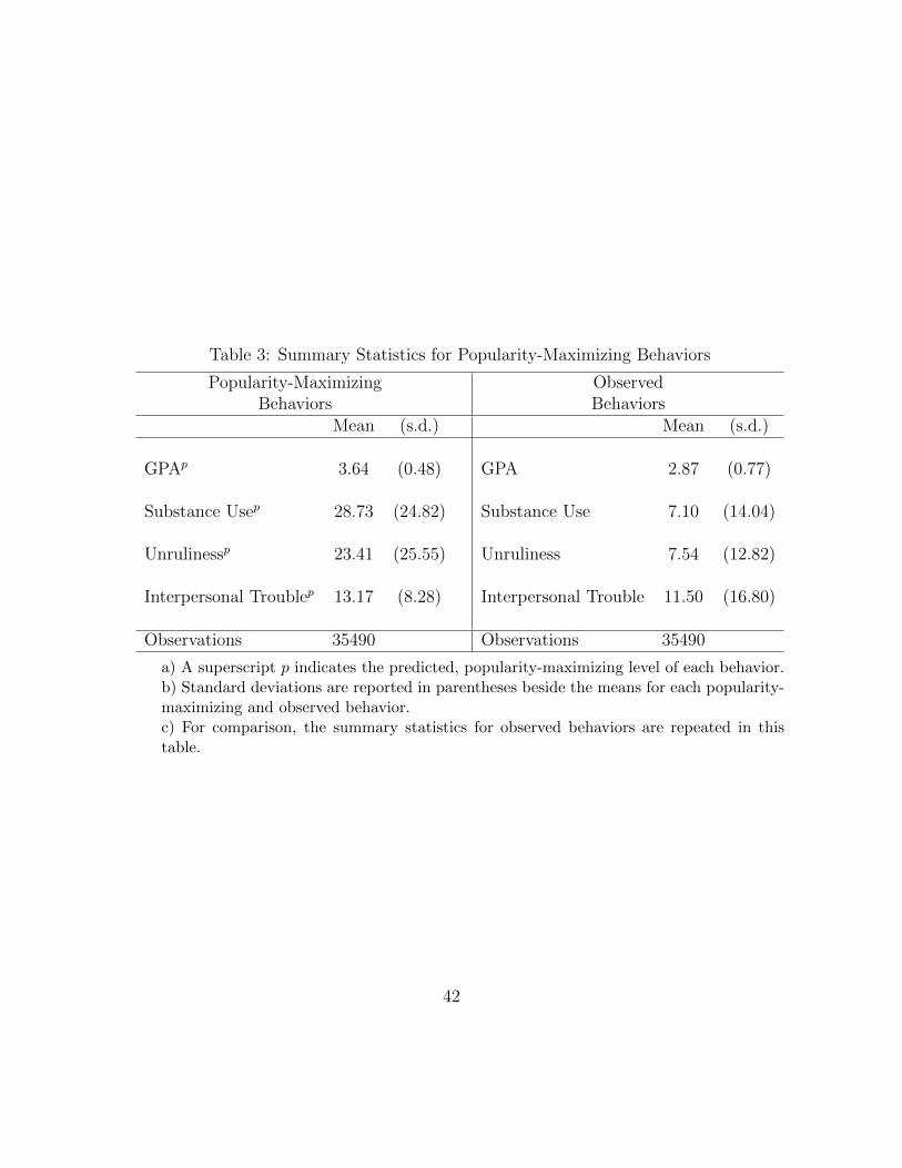
Table 3: Summary Statistics for Popularity-Maximizing Behaviors

Popularity-Maximizing ObservedBehaviors Behaviors

Mean (s.d.) Mean (s.d.)

GPAp 3.64 (0.48) GPA 2.87 (0.77)

Substance Usep 28.73 (24.82) Substance Use 7.10 (14.04)

Unrulinessp 23.41 (25.55) Unruliness 7.54 (12.82)

Interpersonal Troublep 13.17 (8.28) Interpersonal Trouble 11.50 (16.80)

Observations 35490 Observations 35490

a) A superscript p indicates the predicted, popularity-maximizing level of each behavior.b) Standard deviations are reported in parentheses beside the means for each popularity-maximizing and observed behavior.c) For comparison, the summary statistics for observed behaviors are repeated in thistable.

42

Table 4: Relating Utility and Popularity

Variable Happy at School Depressed

Predicted Popularity 0.04*** -0.03***(0.01) (0.01)

Age -0.05*** 0.02*(0.01) (0.01)

Male 0.16*** -0.58***(0.02) (0.02)

Hispanic 0.01 0.04(0.03) (0.03)

White 0.07* 0.11***(0.04) (0.02)

Black -0.22*** -0.12***(0.05) (0.03)

Asian -0.05 0.11***(0.04) (0.03)

Indian -0.15*** 0.22***(0.04) (0.03)

Other Race -0.04* 0.08***(0.02) (0.03)

Years at School 0.02* -0.000(0.01) (0.01)

Mother’s Education 0.02*** -0.001(0.004) (0.003)

Lives with Dad 0.08*** -0.12***(0.02) (0.02)

R-squared 0.02 0.07N. Observations 35,167 35,357N. Schools 88 88

a) The regressions also control for school and grade fixedeffects, as well as all possible interactions between individualcharacteristics and the average characteristics in the school.Standard errors are listed in parentheses. One, two, andthree asterisks indicate statistical significance at the 10-, 5-,and 1-percent level, respectively.b) The table reports bootstrap standard errors

43

Table 5: First Stage Results From 2SLS Estimation of Behavioral Equations(First IV Strategy: School-Composition)

GPAp Substance Usep Unrulinessp Interpersonal Troublep

White*White 0.12*** -14.04*** -42.14*** 10.76***(0.02) (1.48) (0.98) (0.39)

Black*Black 0.34*** 14.10*** -28.67*** -4.72***(0.03) (2.13) (1.42) (0.56)

Hispanic*Hispanic 0.20*** 4.47** -55.21*** 11.28***(0.03) (2.11) (1.40) (0.56)

Asian*Asian 0.02 -17.56*** -19.76*** -15.93***(0.05) (3.17) (2.11) (0.84)

Mom’s Edu*Mom′sEdu -0.003*** -0.01 -1.01*** 0.06***(0.001) (0.06) (0.04) (0.02)

With Dad*WithDad 0.03 -5.10 -53.04*** 0.79(0.05) (3.40) (2.26) (0.90)

Age -0.02*** 0.84*** 0.29** 0.19***(0.003) (0.20) (0.14) (0.05)

Male -0.07*** 2.54*** -2.88*** -2.83***(0.004) (0.24) (0.16) (0.06)

Hispanic -0.04*** 2.05*** -1.43*** -0.23(0.01) (0.65) (0.43) (0.17)

White -0.01 5.01*** 9.26*** -0.19(0.02) (1.05) (0.70) (0.28)

Black -0.08*** -2.77*** -15.67*** 4.73***(0.01) (0.80) (0.53) (0.21)

Asian -0.001 -3.93*** 0.16 -1.53***(0.01) (0.84) (0.56) (0.22)

Indian 0.02** -1.60*** 4.86*** -5.00***(0.01) (0.59) (0.39) (0.16)

Other Race -0.01 -1.24** -5.88*** 3.45***(0.01) (0.53) (0.35) (0.14)

Years at School -0.001 -0.14 0.05 -0.05(0.002) (0.13) (0.09) (0.04)

Mother’s Education 0.04*** 0.43 6.63*** 0.15(0.01) (0.81) (0.54) (0.21)

Lives with Dad -0.05 1.10 27.25*** 0.26(0.04) (2.70) (1.79) (0.71)

Constant 3.88*** 17.49*** 155.62*** -10.34***(0.06) (3.72) (2.47) (0.98)

R-squared 0.03 0.03 0.65 0.34N. Observations 35,490 35,490 35,490 35,490N. Schools 88 88 88 88F-statistic on Excluded IV’s 44.66*** 26.34*** 1271.30** 262.78***F(6, 35382)

a) Behaviors are estimated, popularity-maximizing levels for each student. Excluded IV’s are interac-tions between the student’s own characteristic and the school average, denoted with a bar over them.Regressions control for school and grade fixed effects (12th grade is excluded). Standard errors arelisted in parentheses. One, two, and three asterisks indicate statistical significance at the 10-, 5-, and1-percent level, respectively.

44

Table 6: First Stage Results From 2SLS Estimation of Behavioral Equations (Second IVStrategy: Grade-Composition)

GPAp Substance Usep Unrulinessp Interpersonal Troublep

White*Whitegs -0.05 2.06 -19.80*** 4.15***(0.05) (2.90) (1.92) (0.76)

Black*Blackgs 0.47*** -11.85*** -23.00*** 2.55**(0.07) (4.48) (2.98) (1.18)

Hispanic*Hispanicgs -0.02 -3.73 -41.08*** 5.06***(0.10) (6.15) (4.08) (1.62)

Asian*Asiangs 0.05 -9.61 -14.42*** -6.57***(0.12) (7.56) (5.02) (1.99)

Mom’s Edu*Mom′sEdugs 0.004*** -0.20*** -0.21*** -0.10***(0.001) (0.04) (0.02) (0.01)

With Dad*WithDadgs 0.14*** -5.25* -19.35*** -1.78**(0.05) (3.11) (2.07) (0.82)

Age -0.02*** 0.82*** 0.30** 0.19***(0.003) (0.20) (0.14) (0.05)

Male -0.07*** 2.52*** -2.87*** -2.83***(0.004) (0.24) (0.16) (0.06)

Hispanic -0.04*** 2.20*** -1.23*** -0.23(0.01) (0.65) (0.43) (0.17)

White -0.01 4.68*** 9.03*** -0.14(0.02) (1.05) (0.70) (0.28)

Black -0.09*** -2.09*** -14.98*** 4.53***(0.01) (0.79) (0.53) (0.21)

Asian -0.002 -3.80*** 0.32 -1.55***(0.01) (0.85) (0.56) (0.22)

Indian 0.02** -1.53*** 4.91*** -5.02***(0.01) (0.59) (0.39) (0.16)

Other Race -0.01 -1.22** -5.85*** 3.44***(0.01) (0.53) (0.35) (0.14)

Years at School -0.0004 -0.15 0.04 -0.05(0.002) (0.13) (0.09) (0.04)

Mother’s Education 0.05*** 0.62 6.76*** 0.21(0.01) (0.80) (0.53) (0.21)

Lives with Dad -0.07 0.27 25.58*** 0.77(0.04) (2.70) (1.79) (0.71)

White*White−gs 0.17*** -15.45*** -21.66*** 6.50***(0.05) (2.95) (1.96) (0.78)

Black*Black−gs -0.13* 23.69*** -7.90*** -6.42***(0.07) (4.39) (2.91) (1.15)

Hispanic*Hispanic−gs 0.21** 7.72 -13.84*** 6.24***(0.10) (6.09) (4.05) (1.60)

Asian*Asian−gs -0.04 -7.95 -5.42 -9.18***(0.12) (7.90) (5.25) (2.08)

Mom’s Edu*Mom′sEdu−gs -0.01*** 0.17*** -0.81*** 0.16***(0.001) (0.05) (0.04) (0.01)

With Dad*WithDad−gs -0.09 1.23 -31.51*** 1.94*(0.06) (3.79) (2.52) (1.00)

Constant 3.87*** 17.68*** 155.48*** -10.42***(0.06) (3.71) (2.47) (0.98)

Observations 35,490 35,490 35,490 35,490R-squared 0.04 0.03 0.65 0.34Number of Schools 88 88 88 88F-statistic on Excluded IV’s, F(6, 35382) 17.74*** 7.55*** 86.51*** 29.11***

a) The behaviors are the estimated, popularity-maximizing levels for each student. The excluded IV’s are inter-actions between the student’s own characteristic and the school-grade average characteristic, denoted here with abar over them. A subscript of “-g” indicates an average taken over all other grades in the school. The regressionsalso control for school fixed effects and grade fixed effects (12th grade is the excluded category). Standard errorsare listed in parentheses. One, two, and three asterisks indicate statistical significance at the 10-, 5-, and 1-percentlevel, respectively. 45

Table 7: Behavioral Results – GPA

GPA 2SLS 2SLSOLS School FE (IV-Strategy 1) (IV-Strategy 2)

GPAp 0.26*** 0.09*** 0.21* 0.34*(0.01) (0.01) (0.12) (0.20)

Age -0.15*** -0.15*** -0.15*** -0.014***(0.01) (0.01) (0.01) ( 0.01)

Male -0.10*** -0.13*** -0.12*** -0.12***(0.01) (0.01) (0.01) (0.02)

Hispanic -0.12*** -0.10*** -0.10*** -0.13***(0.01) (0.02) (0.02) (0.02)

White 0.02* 0.04*** 0.03** -0.01(0.02) (0.02) (0.02) (0.03)

Black -0.20*** -0.20*** -0.20*** -0.13***(0.02) (0.02) (0.02) (0.03)

Asian 0.21*** 0.26*** 0.26*** 0.30***(0.02) (0.02) (0.02) (0.03)

Indian -0.10*** -0.11*** -0.11*** -0.11***(0.02) (0.02) (0.02) (0.02)

Other Race -0.04*** -0.04** -0.04** -0.04**(0.02) (0.02) (0.02) (0.02)

Years at School 0.02*** 0.01 0.01 0.01(0.003) (0.004) (0.004) (0.004)

Mom’s Education 0.05*** 0.05*** 0.05*** 0.03(0.002) (0.002) (0.002) (0.03)

Lives with Dad 0.15*** 0.14*** 0.14*** -0.18**(0.01) (0.01) (0.01) (0.08)

Constant 3.78*** 4.36*** 3.88*** 3.37***(0.12) (0.13) (0.50) (0.78)

R-squared 0.15 0.09N. Observations 35,490 35,490 35,490 35,490N. Schools 88 88 88 88

a) Standard errors are listed in parentheses below the coefficient estimates. One, two, and three asterisksindicate statistical significance at the 10- , 5- , and 1-percent level, respectively. The 2SLS procedurecontrols for school fixed effects. All specifications also control for grade fixed effects. A superscript pdenotes the popularity-maximizing level of the behavior.b) IV-strategy 1 uses interaction terms between individual characteristics and school averages as theexcluded instruments. IV-strategy 2 uses interaction terms between individual characteristics and grade-school specific averages for identification.

46

Table 8: Behavioral Results – Substance Use

Substance Use 2SLS 2SLSOLS School FE (IV-strategy 1) (IV-strategy 2)

Substance Usep 0.05*** 0.03*** 0.11** 0.28***(0.003) (0.003) (0.05) (0.10)

Age 1.78*** 1.81*** 1.74*** 1.60***(0.12) (0.13) (0.13) (0.16)

Male 1.07** 1.04*** 0.83*** 0.39(0.15) (0.15) (0.20) (0.30)

Hispanic -1.13*** 0.35 0.07 1.29***(0.27) (0.30) (0.34) (0.48)

White 2.27*** 2.01*** 2.33*** 2.76***(0.29) (0.29) (0.35) (0.85)

Black -2.98*** -3.28*** -3.35*** -3.45***(0.33) (0.35) (0.36) (0.58)

Asian -0.44 -0.27 0.33 -0.29(0.37) (0.38) (0.53) (0.69)

Indian 3.13*** 3.13*** 3.23*** 3.39***(0.37) (0.37) (0.37) (0.42)

Other Race 1.04*** 1.17*** 1.26*** 1.50***(0.33) (0.33) (0.34) (0.37)

Years at School 0.02 -0.004 0.01 0.04(0.06) (0.08) (0.09) (0.09)

Mom’s Education -0.21*** -0.21*** -0.24*** 0.23(0.03) (0.03) (0.04) (0.50)

Lives with Dad -2.14*** -2.29*** -2.04*** 3.22*(0.19) (0.19) (0.25) (1.72)

Constant -21.10*** -20.93*** -22.33*** -24.38***(2.24) (2.32) (2.48) (3.06)

R-squared 0.04 0.03N. Observations 35,490 35,490 35,490 35,490N. Schools 88 88 88 88

a) Standard errors are listed in parentheses below the coefficient estimates. One, two, and three asterisksindicate statistical significance at the 10- , 5- , and 1-percent level, respectively. The 2SLS procedurecontrols for school fixed effects. All specifications also control for grade fixed effects. A superscript pdenotes the popularity-maximizing level of the behavior.b) IV-strategy 1 uses interaction terms between individual characteristics and school averages as theexcluded instruments. IV-strategy 2 uses interaction terms between individual characteristics and grade-school specific averages for identification.

47

Table 9: Behavioral Results – Unruliness

Unruliness 2SLS 2SLSOLS School FE (IV-strategy 1) (IV-strategy 2)

Unrulinessp 0.06*** 0.06*** 0.06*** 0.08**(0.004) (0.004) (0.01) (0.04)

Age 0.34*** 0.36*** 0.37*** 0.36***(0.11) (0.12) (0.12) (0.12)

Male 3.09*** 3.18*** 3.17*** 3.22***(0.14) (0.14) (0.14) (0.18)

Hispanic 2.28*** 2.11*** 2.06*** 2.39***(0.26) (0.28) (0.30) (0.38)

White 1.06*** 1.29*** 1.22*** 2.06***(0.27) (0.28) (0.31) (0.66)

Black 1.68*** 1.28*** 1.19*** 0.42(0.32) (0.33) (0.38) (0.73)

Asian -0.28 0.17 0.17 -0.43(0.33) (0.35) (0.35) (0.48)

Indian 2.49*** 2.38*** 2.41*** 2.31***(0.34) (0.34) (0.35) (0.39)

Other Race 1.13*** 1.11*** 1.09*** 1.23***(0.30) (0.30) (0.31) (0.37)

Years at School -0.07 -0.002 -0.002 -0.002(0.06) (0.08) (0.08) (0.08)

Mom’s Education 0.25*** 0.28*** 0.25*** 0.70(0.04) (0.04) (0.08) (0.45)

Lives with Dad -0.27 -0.23 -0.29 -0.362**(0.19) (0.19) (0.23) (1.63)

Constant -6.76*** -7.95*** -7.289*** -10.08(2.13) (2.22) (2.57) (6.28)

R-squared 0.03 0.03N. Observations 35,490 35,490 35,490N. Schools 88 88 88

a) Standard errors are listed in parentheses below the coefficient estimates. One, two, and three asterisksindicate statistical significance at the 10- , 5- , and 1-percent level, respectively. The 2SLS procedurecontrols for school fixed effects. All specifications also control for grade fixed effects. A superscript pdenotes the popularity-maximizing level of the behavior.b) IV-strategy 1 uses interaction terms between individual characteristics and school averages as theexcluded instruments. IV-strategy 2 uses interaction terms between individual characteristics and grade-school specific averages for identification.

48

Table 10: Behavioral Results – Interpersonal Trouble

Interpersonal Trouble 2SLS 2SLSOLS School FE (IV-strategy 1) (IV-strategy 2)

Interpersonal Troublep 0.13*** 0.04*** -0.28*** 0.29(0.01) (0.02) (0.07) (0.22)

Age 2.42*** 2.39*** 2.45*** 2.33***(0.15) (0.15) (0.15) (0.157)

Male 2.52*** 2.28*** 1.36*** 2.96***(0.18) (0.18) (0.27) (0.63)

Hispanic 1.28*** 1.13*** 1.83*** 2.59***(0.33) (0.36) (0.39) (0.48)

White -3.01*** -2.51*** -0.43 -2.50***(0.35) (0.36) (0.58) (0.77)

Black 1.68*** 2.23*** 3.22*** 1.93*(0.40) (0.42) (0.48) (1.13)

Asian 2.05*** 1.61*** -0.003 0.46(0.44) (0.46) (0.58) (0.73)

Indian 2.08*** 1.64*** -0.09 2.82**(0.44) (0.44) (0.58) (1.17)

Other Race -0.05 0.13 1.28*** -0.66(0.39) (0.40) (0.47) (0.84)

Years at School -0.03 0.07 0.06 0.08(0.08) (0.10) (0.10) (0.10)

Mom’s Education -0.59*** -0.43*** -0.12 -0.87(0.04) (0.04) (0.08) (0.56)

Lives with Dad -1.06*** -0.79*** -0.48** 2.52(0.23) (0.23) (0.24) (1.91)

Constant -24.63*** -26.22*** -28.87*** -22.94***(2.67) (2.77) (2.84) (3.56)

R-squared 0.05 0.03N. Observations 35,490 35,490 35,490 35,490N. Schools 88 88 88 88

a) Standard errors are listed in parentheses below the coefficient estimates. One, two, and three asterisks indicatestatistical significance at the 10- , 5- , and 1-percent level, respectively. The 2SLS procedure controls for schoolfixed effects. All specifications also control for grade fixed effects. A superscript p denotes the popularity-maximizing level of the behavior.b) IV-strategy 1 uses interaction terms between individual characteristics and school averages as the excludedinstruments. IV-strategy 2 uses interaction terms between individual characteristics and grade-school specificaverages for identification.

49

Figure 1: Predicted & Actual Academic Grades Across Student Types & Schools

a) The three panels, separated by the dotted lines, show behaviors for students in three different schools. Diamonds

indicate the predicted behavior for the three types of students across the schools. Small circles represent observations

in the data for students in the school who match the description of the hypothetical student.

b) All three hypothetical students are 15 years old, in 10th grade, and have been at the school for 2 years. The

race, gender, and socioeconomic status of each hypothetical student are listed along the horizontal axis. High

socioeconomic status corresponds with having a mother who holds at least a master’s degree and having a father

present in the household. Median socioeconomic status refers to a having a mother who has completed high school

but does not have a college degree, and having a father present.

50

Figure 2: Predicted and Actual Substance Use Across Student Types and Schools

a) The three panels, separated by the dotted lines, show behaviors for students in three different schools. Diamonds

indicate the predicted behavior for the three types of students across the schools. Small circles represent observations

of behaviors in the data for students in the school who match the description of the hypothetical student.

b) All three hypothetical students are 15 years old, in 10th grade, and have been at the school for 2 years. The

race, gender, and socioeconomic status of each hypothetical student are listed along the horizontal axis. High

socioeconomic status corresponds with having a mother who holds at least a master’s degree and having a father

present in the household. Median socioeconomic status refers to a having a mother who has completed high school

but does not have a college degree, and having a father present.

51

Figure 3: Predicted and Actual Unruly Behavior Across Student Types and Schools

a) The three panels, separated by the dotted lines, show behaviors for students in three different schools. Diamonds

indicate the predicted behavior for the three types of students across the schools. Small circles represent observations

of behaviors in the data for students in the school who match the description of the hypothetical student.

b) All three hypothetical students are 15 years old, in 10th grade, and have been at the school for 2 years. The

race, gender, and socioeconomic status of each hypothetical student are listed along the horizontal axis. High

socioeconomic status corresponds with having a mother who holds at least a master’s degree and having a father

present in the household. Median socioeconomic status refers to a having a mother who has completed high school

but does not have a college degree, and having a father present.

52

7 Appendix: Bivariate Probit Results

Table 11: Bivariate Probit ResultsProbability that Person j Nominates Person i

General “Coolness” in BehaviorsBehaviors (yi, y

2i )

GPA -0.14233211***(0.017)

Substance Use 0.00354063***(0.001)

Unruliness 0.00038622(0.001)

Interpersonal Trouble 0.00111946*(0.001)

GPA2 0.01551107***(0.002)

Substance Use2 0.00000983*(0.000)

Unruliness2 0.00000429(0.000)

Interpersonal Trouble2 -0.00000246(0.000)

Homophily in BehaviorsDistance in Behaviors ((yi − yj)2)GPA-distance -0.05503049***

(0.002)Substance Use-distance -0.00008118***

(0.000)Unruliness-distance -0.00001013***

(0.000)Interpersonal Trouble-distance -0.00001517***

(0.000)Interactions in Behaviors (yi ∗ yj)GPA-interaction 0.01362604***

(0.001)Substance Use-interaction 0.00013761***

(0.000)Unruliness-interaction 0.00000732

(0.000)Interpersonal Trouble-interaction -0.00000146

(0.000)

(CONTINUED)

53

Table 1.11 Continued: Bivariate Probit ResultsProbability that Person j Nominates Person i

Characteristics of the NomineeCharacteristics (xi, x

2i )

Age 0.04870483(0.031)

Male 0.05380015***(0.014)

Hispanic -0.04275485*(0.025)

White -0.07837962***(0.027)

Black -0.08066360**(0.037)

Asian 0.00856091(0.037)

Indian -0.05710053*(0.030)

Other Race -0.04606534*(0.027)

Years at School 0.07843586***(0.006)

Lives With Dad 0.03763856**(0.019)

Mother’s Education 0.00202729(0.006)

Age2 -0.00154896(0.001)

Years at School2 -0.00976036***(0.001)

Mom’s Education2 0.00056820***(0.000)

(CONTINUED)

54

Table 1.11 Continued: Bivariate Probit ResultsProbability that Person j Nominates Person i

Homophily in CharacteristicsDistance in Characteristics ((xi − xj)2)Grade-distance -0.04185820***

(0.002)Age-distance -0.01648061***

(0.001)Male-distance -0.13381297***

(0.015)Hispanic-distance 0.02085278

(0.026)White-distance -0.04073913

(0.028)Black-distance -0.25858481***

(0.037)Asian-distance -0.10304419***

(0.037)Indian-distance 0.04920090*

(0.029)Other Race-distance 0.03929546

(0.027)Years at School-distance -0.00673962***

(0.001)Lives with Dad-distance -0.03822054*

(0.020)Mom’s Education-distance -0.00292635***

(0.000)Interactions in Characteristics (xi ∗ xj)Age-interaction -0.00075587***

(0.000)Male-interaction -0.07089025***

(0.023)Hispanic-interaction 0.24070085***

(0.046)White-interaction 0.14308518***

(0.048)Black-interaction 0.30389580***

(0.058)Asian-interaction 0.35002329***

(0.070)Indian-interaction 0.12764530

(0.116)Other Race-interaction 0.09444958

(0.065)Years at School-interaction 0.00547474***

(0.000)Lives with Dad-interaction -0.01162758

(0.031)Mom’s Education-interaction -0.00038033**

(0.000)9th Grade-interaction 0.76549501***

(0.008)10th Grade-interaction 0.67152154***

(0.006)11th Grade-interaction 0.60153644***

(0.006)12th Grade-interaction 0.58258758***

(0.008)

(CONTINUED)55

Table 1.11 Continued: Bivariate Probit ResultsProbability that j Nominates i

Varying Perceptions of “Cool” Behaviors by Characteristics of the Nominator - GPAInteractions Between Nominator’s Characteristics & Nominee’s Behavior (xj ∗ yi)Male-GPA 0.02295788***

(0.004)Hispanic-GPA -0.02015993**

(0.008)White-GPA -0.02046619**

(0.008)Black-GPA -0.03629561***

(0.011)Asian-GPA 0.00742348

(0.011)Indian-GPA -0.02007624**

(0.009)Other Race-GPA -0.00523329

(0.008)Lives with Dad-GPA 0.01188473**

(0.006)Mom’s Education-GPA 0.00456669***

(0.001)

Interactions of Nominator’s & Nominee’s Characteristics, & Nominee’s Behavior (xj ∗ xi ∗ yi)Male-Male-GPA -0.01482142***

(0.005)Hispanic-Hispanic-GPA 0.02512044**

(0.011)White-White-GPA 0.00891471

(0.006)Black-Black-GPA 0.04419077***

(0.011)Asian-Asian-GPA -0.03195628*

(0.017)Indian-Indian-GPA 0.05809285*

(0.035)Other Race-Other Race-GPA 0.00346160

(0.020)Lives with Dad-Lives with Dad-GPA -0.00370797

(0.005)Mom’s Education-Mom’s Education-GPA -0.00001416

(0.000)

(CONTINUED)

56

Table 1.11 Continued: Bivariate Probit ResultsProbability that j Nominate i

Varying Perceptions of “Cool” Behaviors by Characteristics of the Nominator - Substance UseInteractions Between Nominator’s Characteristics & Nominee’s Behavior (xj ∗ yi)Male-Substance Use -0.00054331**

(0.000)Hispanic-Substance Use -0.00020388

(0.001)White-Substance Use 0.00026357

(0.001)Black-Substance Use -0.00176891**

(0.001)Asian-Substance Use -0.00165487**

(0.001)Indian-Substance Use 0.00086756

(0.001)Other Race-Substance Use 0.00085307

(0.001)Lives with Dad-Substance Use -0.00005873

(0.000)Mom’s Education-Substance Use -0.00024887***

(0.000)

Interactions of Nominator’s & Nominee’s Characteristics, & Nominee’s Behavior (xj ∗ xi ∗ yi)Male-Male-Substance Use 0.00025390

(0.000)Hispanic-Hispanic-Sustance Use 0.00096450

(0.001)White-White-Substance Use -0.00054887

(0.000)Black-Black-Substance Use 0.00268157***

(0.001)Asian-Asian-Substance Use -0.00063008

(0.001)Indian-Indian-Substance Use -0.00400246*

(0.002)Other Race-Other Race-Substance Use -0.00112316

(0.001)Lives with Dad-Lives with Dad-Substance Use -0.00026279

(0.000)Mom’s Education-Mom’s Education-Substance Use 0.00000577*

(0.000)

(CONTINUED)

57

Table 1.11 Continued: Bivariate Probit ResultsProbability that j Nominates i

Varying Perceptions of “Cool” Behaviors by Characteristics of the Nominator - UnrulinessInteractions Between Nominator’s Characteristics & Nominee’s Behavior (xj ∗ yi)Male-Unruliness 0.00033803

(0.000)Hispanic-Unruliness -0.00029864

(0.001)White-Unruliness -0.00031634

(0.001)Black-Unruliness -0.00072003

(0.001)Asian-Unruliness -0.00014430

(0.001)Indian-Unruliness -0.00062938

(0.001)Other Race-Unruliness -0.00040016

(0.001)Lives with Dad-Unruliness 0.00000532

(0.000)Mom’s Education-Unruliness 0.0015907**

(0.000)

Interactions of Nominator’s & Nominee’s Characteristics, & Nominee’s Behavior (xj ∗ xi ∗ yi)Male-Male-Unruliness -0.00017156

(0.000)Hispanic-Hispanic-Unruliness -0.00083765

(0.001)White-White-Unruliness -0.00045553

(0.000)Black-Black-Unruliness -0.00069326

(0.001)Asian-Asian-Unruliness -0.00045232

(0.001)Indian-Indian-Unruliness 0.00065168

(0.002)Other Race-Other Race-Unruliness -0.00093372

(0.001)Lives with Dad-Lives with Dad-Unruliness -0.00028295

(0.000)Mom’s Education-Mom’s Education-Unruliness -0.00000889***

(0.000)

(CONTINUED)

58

Table 1.11 Continued: Bivariate Probit ResultsProbability that j Nominates i

Varying Perceptions of “Cool” Behaviors by Characteristics of the Nominator - TroubleInteractions Between Nominator’s Characteristics & Nominee’s Behavior (xj ∗ yi)Male-Interpersonal Trouble -0.00012521

(0.000)Hispanic-Interpersonal Trouble 0.00008857

(0.000)White-Interpersonal Trouble -0.00034147

(0.000)Black-Interpersonal Trouble 0.00073576

(0.001)Asian-Interpersonal Trouble 0.00013171

(0.001)Indian-Interpersonal Trouble 0.00093555**

(0.000)Other Race-Interpersonal Trouble -0.00073496*

(0.000)Lives with Dad-Interpersonal Trouble -0.00021189

(0.000)Mom’s Education-Interpersonal Trouble -0.00011108**

(0.000)

Interactions of Nominator’s & Nominee’s Characteristics, & Nominee’s Behavior (xj ∗ xi ∗ yi)Male-Male-Interpersonal Trouble -0.00020825

(0.000)Hispanic-Hispanic-Interpersonal Trouble 0.00026008

(0.000)White-White-Interpersonal Trouble 0.00051352**

(0.000)Black-Black-Interpersonal Trouble -0.00043573

(0.000)Asian-Asian-Interpersonal Trouble -0.00066907

(0.001)Indian-Indian-Interpersonal Trouble -0.00304771*

(0.002)Other Race-Other Race-Interpersonal Trouble 0.00085060

(0.001)Lives with Dad-Lives with Dad-Interpersonal Trouble 0.00006204

(0.000)Mom’s Education-Mom’s Education-Interpersonal Trouble 0.00000331

(0.000)Constant -3.20359793***

(0.255)

ρ 0.82Observations 643,293

a) Standard errors are listed in parenthesis below the coefficient estimates. One, two, andthree asterisks indicate statistical significance at the 10- , 5- , and 1-percent level, respec-tively.b) It is random whether a student is indexed with an i or a j. Both equations in the bivariateprobit have identical specifications, as noted in equation (7). As a result, the coefficientestimates for the probability of person i nominating person j have been constrained to beidentical to those reported in the above table.

59

References

[1] Akerloff, George A. and Rachel E. Kranton. “Economics and Identity.” TheQuarterly Journal of Economics, 115, no. 4 (2000): 715-753.

[2] Akerloff, George A. and Rachel E. Kranton. “Identity and Schooling: SomeLessons for the Economics of Education.” The Journal of Economic Literature,40, no. 4 (2002): 117-1201.

[3] Alesina, Alberto and Eliana La Ferrara. “Participation in Heterogeneous Com-munities.” The Quarterly Journal of Economics, 115, no. 3 (2000): 847-904.

[4] Babcock, Philip. “From Ties to Gains? Evidence of Connectedness and HumanCapital Acquisition.” Journal of Human Capital, 4, no. 4 (2008): 379-409.

[5] Calvo-Armengol, Antoni, Eleonra Patacchini, and Yves Zenou. “Peer Effectsand Social Networks in Education.” The Review of Economic Studies, 79 (2009):1239-1267.

[6] Carrell, Scott E., Bruce I. Sarcerdote, and James E. West. “From Natural Vari-ation to Optimal Policy? The Importance of Endogenous Peer Group Forma-tion.” Econometrica, 81, no. 3 (2013): 855-882.

[7] Conti, Gabriella, Andrea Galeotti, Gerrit Mueller, and Stephen Pudney. “Pop-ularity.” Working Paper (2011): 1-28.

[8] Currarini, Sergio, Matthew O. Jackson, and Paolo Pin. “An Economic Modelof Friendship, Minorities, and Segregation.” Econometrica, 77, no. 4 (2009):1003-1045.

[9] Foster, Gigi. “Making Friends: A nonexperimental analysis of social pair forma-tion.” Human Relations, 58 (2005): 1443-1465.

[10] Foster, Gigi. “It’s not your peers, and it’s not your friends: Some progresstoward understanding the education peer effect mechanisms.” Journal of PublicEconomics, 90 (2006): 1455-1475.

[11] Glaeser, Edward L., Bruce I. Sacerdote, Jose A. Scheinkman. “The Social Mul-tiplier.” NBER Working Paper, No. 9153 (2002): 1-25.

60

[12] Goldsmith-Pinkham, Paul and Guido W. Imbeds. “Social Networks and theIdentification of Peer Effects.” Journal of Business & Economic Statistics, 31,no. 3 (2013): 253-264.

[13] Haynie, Dana. “Delinquent Peers Revisited: Does Network Structure Matter?”American Journal of Sociology, 106, no. 4 (2001): 1013-1057.

[14] Hoxby, Caroline. “Peer Effects in the Classroom: Learning from Gender andRace Variation.” Working Paper (2000): 1-64.

[15] Kandel, Denise B. “Homophily, Selection, and Socialization in AdolescentFriendships.” American Journal of Sociology, 84, no. 2 (1978): 427-436.

[16] Katz, Lawrence F., Jeffrey R. Kling, and Jeffrey B. Liebman. “Moving to Op-portunity in Boston: Early Results of a Randomized Mobility Experiment.” TheQuarterly Journal of Economics, 116, no. 2 (2001): 607-654.

[17] Kiefer, Sarah M. and Allison M. Ryan. “Striving for Social Dominance OverPeers: The Implications for Academic Adjustment During Early Adolescence.”Journal of Educational Pyschology, 100, no. 2 (2008): 417-428.

[18] Kuhn, Peter and Catherine J. Weinberger. “Leadership Skills and Wages.”Working Paper (2002): 1-54.

[19] Lin, Xu and Bruce Weinberg. “Unrequited Friendship? How Reciprocity Medi-ates Adolescent Peer Effects.” Working Paper (2013): 1-23.

[20] Lyle, David S. “Estimating and Interpreting peer and Role Model Effects fromRandomly Assigned Social Groups at West Point.” The Review of Economicsand Statistics, 89, no. 2 (2007): 289-299.

[21] Manski, Charles. “Identification of Endogenous Social Effects: The ReflectionProblem.” The Review of Economic Studies, 60, no. 3 (1993): 531-542.

[22] Massey, Douglas S. and Nancy A. Denton. “Hypersegregation in U.S. Metropoli-tan Areas: Black and Hispanic Segregation along Five Dimensions.” Demogra-phy, 26, no. 3 (1989): 373-391.

[23] Mihaly, Kata. “Do More Friends Mean Better Grades?” Working Paper (2009):1-29.

[24] Pfeifer, Christian. “Physical Attractiveness, Employment, and Earnings.” Ap-plied Economic Letters, 19, no. 6 (2012): 505-510.

61

[25] Putnam, Robert D. “Bowling Alone: America’s Declining Social Capital.” Jour-nal of Democracy, 6, no. 1 (1995): 65-78.

[26] Sarcedote, Bruce. “Peer Effects with Random Assignment: Results for Dart-mouth Roommates.” The Quarterly Journal of Economics, 116, no. 2 (2001):681-704.

[27] Steele, Claude M. “A Threat in the Air: How Stereotypes Shape IntellectualIdentify and Performance.” American Psychologist, 52, no. 6 (1997): 613-629.

[28] Stinebrickner, Ralph and Todd R. Stinebrickner. “What can be learned aboutpeer effects using college roommates? Evidence from new survey data andstudents from disadvantaged backgrounds.” Journal of Public Economics, 90(2006): 1435-1454.

[29] Weinberg, Bruce. “Social Interactions and Endogenous Associations.” WorkingPaper (2008): 1-53.

[30] Zimmerman, David. “Peer Effects in Academic Outcomes: Evidence from aNatural Experiment.” The Review of Economics and Statistics, 85, no. 1 (2003):9-23.

62