the race between education and technology: the … · the race between education and technology:...

NBER WORKING PAPER SERIES

THE RACE BETWEEN EDUCATION AND TECHNOLOGY: THE EVOLUTION OF U.S. EDUCATIONAL WAGE DIFFERENTIALS, 1890 TO 2005

Claudia Goldin

Lawrence F. Katz

Working Paper 12984 http://www.nber.org/papers/w12984

NATIONAL BUREAU OF ECONOMIC RESEARCH 1050 Massachusetts Avenue

Cambridge, MA 02138 March 2007

This paper is Chapter 8 of our book, The Intimate Contest between Education and Technology (tentative title; forthcoming 2008). The views expressed herein are those of the author(s) and do not necessarily reflect the views of the National Bureau of Economic Research. © 2007 by Claudia Goldin and Lawrence F. Katz. All rights reserved. Short sections of text, not to exceed two paragraphs, may be quoted without explicit permission provided that full credit, including © notice, is given to the source.

The Race between Education and Technology: The Evolution of U.S. Educational Wage Differentials,1890 to 2005Claudia Goldin and Lawrence F. KatzNBER Working Paper No. 12984March 2007JEL No. I2,J2,J3,N3,O3

ABSTRACT

U.S. educational and occupational wage differentials were exceptionally high at the dawn of the twentiethcentury and then decreased in several stages over the next eight decades. But starting in the early 1980sthe labor market premium to skill rose sharply and by 2005 the college wage premium was back atits 1915 level. The twentieth century contains two inequality tales: one declining and one rising. Weuse a supply-demand-institutions framework to understand the factors that produced these changesfrom 1890 to 2005. We find that strong secular growth in the relative demand for more educated workerscombined with fluctuations in the growth of relative skill supplies go far to explain the long-run evolutionof U.S. educational wage differentials. An increase in the rate of growth of the relative supply of skillsassociated with the high school movement starting around 1910 played a key role in narrowing educationalwage differentials from 1915 to 1980. The slowdown in the growth of the relative supply of collegeworkers starting around 1980 was a major reason for the surge in the college wage premium from1980 to 2005. Institutional factors were important at various junctures, especially during the 1940sand the late 1970s.

Claudia GoldinDepartment of EconomicsHarvard UniversityCambridge, MA 02138and [email protected]

Lawrence F. KatzDepartment of EconomicsHarvard UniversityCambridge, MA 02138and [email protected]

The Intimate Contest between Education and Technology Book Outline: Introduction Section I: Economic Growth and Distribution

Chapter 1. The Human Capital Century Chapter 2. Inequality across the Twentieth Century Chapter 3. Skill-biased Technological Change

Section II: Education for the Masses in Three Transformations Chapter 4. The Origins of the Virtues Chapter 5. Economic Foundations of the High School Movement Chapter 6. America’s Graduation from High School Chapter 7. Mass Higher Education in the Twentieth Century

Section III: The Race Chapter 8. The Race between Education and Technology Chapter 9. How America Once Led and Can Win the Race for Tomorrow

Appendix to Chapter 2: Appendix 2 Appendix to Chapter 6: Appendix 6 Appendix to Chapter 6: Appendix 6a Appendix to Chapter 8: Appendix 8 Bibliography

Chapter 8: The Race between Education and Technology Section pages A. Two Tales of the Twentieth Century ...................................................................................... 1

1. The “best poor man’s country” ........................................................................................... 1 2. Integrating the two tales of the twentieth century............................................................... 3

B. The Supply, Demand, and Institutions (SDI) Framework ...................................................... 6 C. Why the Premium to Skill Changed: 1915 to 2005 ................................................................ 8

1. College wage premium ....................................................................................................... 8 a. Applying the framework ................................................................................................. 8 b. Computing supply and demand shifts........................................................................... 12

2. High school wage premium .............................................................................................. 13 a. Applying the framework ............................................................................................... 13 b. Computing supply and demand shifts........................................................................... 16

3. Role of immigration.......................................................................................................... 17 a. Immigration and the labor force ................................................................................... 17 b. Immigration and the skill gap ....................................................................................... 19

D. Non-competing Groups: 1890 to 1930 ................................................................................. 22 1. The premium to skill and the relative supply of educated workers .................................. 22 2. Explaining the skill premium decline: education, immigration, and demand .................. 24

E. Recapitulation: Who Won the Race?.................................................................................... 26 References..................................................................................................................................... 30 Figure 1 ......................................................................................................................................... 32 College Graduate and High School Graduate Wage Premiums: 1915 to 2005 ............................ 32 Figure 2 ......................................................................................................................................... 33 Actual versus Predicted College Wage Premium: 1915 to 2005.................................................. 33 Table 1 .......................................................................................................................................... 34 Changes in the College Wage Premium and the Supply and Demand for College Educated Workers: 1915 to 2005 (100 × Annual Log Changes).................................................................. 34 Table 2 .......................................................................................................................................... 35 Determinants of the College Wage Premium: 1915 to 2005 ........................................................ 35 Table 3 .......................................................................................................................................... 36 Changes in the High School Wage Premium and the Supply and Demand for High School Educated Workers: 1915 to 2005 (100 × Annual Log Changes).................................................. 36 Table 4 .......................................................................................................................................... 37 Determinants of the High School Wage Premium: 1915 to 2005 ................................................ 37 Table 5 .......................................................................................................................................... 39 Immigrant Contribution to Labor Supply by Educational Attainment: 1915 to 2005.................. 39 Table 6 .......................................................................................................................................... 40 Contribution of Immigrants and the U.S. Native-Born to the Growth of Relative Skill Supplies: 1915 to 2005 (100 × Annual Log Changes) ................................................................................. 40 Table 7 .......................................................................................................................................... 41 High School Graduates as a Share of the Labor Force (≥ 14 years old)....................................... 41 Appendix to Chapter 8 (Appendix 8): Construction of Wage Bill Shares and Educational Wage Differentials, 1915 to 2005 ........................................................................................................... 42

A. Two Tales of the Twentieth Century

1. The “best poor man’s country”

Long ago America was deemed the “best poor man’s country.”1 Land was plentiful in

the early nineteenth century and farming provided ample living standards and fairly uniform

incomes. But during the next hundred years the labor force became more diverse. The

population urbanized and the economy industrialized. Had we good income data for the period

we would surely observe that the income distribution had widened considerably from the early

years of the republic to the turn of the twentieth century. But income data for the full

distribution are not available until 1940.2 We do, however, have good data on the wealth

distribution that reveals a great widening.3 By the turn of the twentieth century the distribution

of wealth was extremely unequal.

Despite the lack of thick income data for the pre-1940 period, we know a considerable

amount about the pecuniary returns to education and the premium that accrued to particular

occupations. In the years from around 1890 to 1910 earnings in occupations that required greater

levels of schooling were far higher than those that required little education, as shown in Chapter

2. In addition, the economic return around 1915 to a year of high school or college was

substantial. The return to education in 1915 greatly exceeded that in 1940 and was sufficiently

high that it greatly exceeded returns in subsequent years. Only recently has the college premium

approximated its value in 1915. That is, the payoff to a year of further study in 1915 was

enormously high. We do not know precisely when in the preceding century the premium to

1 The phrase “the best poor man’s country” was initially used in the eighteenth century to describe economic conditions in Pennsylvania but was later used to describe the entire northern part of America. See Lemon (1972, p. 229, fn. 1) who took the title of his book on the early history of southeastern Pennsylvania, The Best Poor Man’s Country, from several contemporary comments about the region. The ideas are similar to those in Tocqueville’s Democracy in America (1981, orig. publ. 1832). 2 See Piketty and Saez (2003, 2006) for data on the incomes of the top 10 percent (or 1 percent) of the distribution from the beginning of the U.S. income tax in 1913 to the early 2000s. 3 James Bryce, in his two volume work The American Commonwealth, remarked that at the time of de Tocqueville “[s]ixty years ago there were no great fortunes in America, few large fortunes, no poverty. Now there is some poverty, many large fortunes, and a greater number of gigantic fortunes than in any other country of the world” (Bryce 1889, p. 600). Bryce was most certainly correct concerning the general trend in wealth accumulation but he was clearly wrong that poverty was nonexistent in the 1830s. On the trend in the wealth distribution from 1776 to the 1920s (1776, 1850, 1860, 1870, and 1920s), see Wolff (1995) and the compilation of wealth data in Nasar (New York Times, August 16, 1992).

The Race between Education and Technology 1

schooling increased and whether it was as high even in 1850. But we do know that by 1900 a

year of high school or college was an extremely good investment.

The large premium to employment in occupations that had substantial educational

requirements around the turn of the twentieth century was observed and commented on by close

contemporaries. The economist Paul Douglas, for one, noted that “during the nineties [1890s],

the clerical class constituted something of a non-competing group.”4 Douglas’s interest in the

wage distribution was sparked by a period of great wage compression that was apparent by the

early 1920s. The astonishing change that took place in his own time prompted his comment:

“Gradually the former monopolistic advantages are being squeezed out of white-collar work, and

eventually there will be no surplus left.”5

According to Douglas several factors were acting in concert to compress wages. One

was the deskilling of clerical workers through the substitution of office machinery for skill.

Another was the reduction in the flow of immigration, which, to Douglas, led to an increase in

the earnings of the less educated. Finally, the supply of educated and trained workers qualified

to assume various white-collar positions greatly increased thus depressing their earnings.

Douglas was correct that there were several factors at work, but the relative increase in the

supply of skilled and educated personnel was of far greater importance than skill reducing factors

on the demand side and also more important than the decrease in immigration, as we shall soon

demonstrate. The possibility that deskilling led to the large decrease in the relative earnings of

the more educated was laid to rest in Chapter 2 when we showed the similarity of wage changes

among clerical occupations. Earnings of white-collar workers in occupations that did not

undergo much technical change were reduced almost as much as those that did undergo

considerable technical change.

The wage structure began to collapse a short time before 1920 and continued to narrow in

various ways until the early 1950s. The earnings of the more educated were reduced relative to

4 Douglas (1930, p. 367, italics added). 5 Douglas (1926, p. 719). Paul Douglas was born in 1892 and would have been in his mid-twenties just as the returns to various skills began to be reduced and the wage distribution started to narrow. He was 34 years old when he wrote about the “non-competing” groups that had previously existed.


the less educated. Those employed in skilled occupations saw their earnings increase less than

did those in the lower-skilled jobs. For every skilled and professional series we uncovered, the

wage structure narrowed relative to wages for a lesser skilled or lower educated group. The

series we presented included professors of all ranks, engineers, office and clerical workers, and

craft positions in many industries. We also found evidence of a substantial narrowing in the

wage distribution of production workers within each of a large group of manufacturing

industries. The returns to a year of schooling, not surprisingly, also plummeted from 1915 to the

early 1950s. Our estimates of the decrease in the pecuniary returns to a year of education are

robust to the level of schooling and also to the age and sex of the individuals. The returns to

schooling were so high prior to the narrowing that even after the initial decline, the returns to

education remained substantial.

Our point is that inequality and the pecuniary returns to education were both

exceptionally high around the turn of the twentieth century. But America remained the

destination of choice for the world’s people, and immigration was at record high levels just

before the 1920s when Congressional legislation severely reduced the flow.6 It was still the

“best poor man’s country,” but the moniker was no longer used because America had a narrow

income distribution. To the contrary, America’s income distribution was probably far wider than

it had ever been. The description was still applicable because America had a considerably higher

average income than did other nations. More important was the fact that the United States was a

society with fairly open educational access and had more equality of opportunity than existed in

Europe. Certain groups, in particular African Americans living in the U.S. South, remained left

out for some time. But even they gained access to improved schooling during the mid-twentieth

century and moved into higher paying jobs in the 1960s.

2. Integrating the two tales of the twentieth century

By the early 1970s one could say that America “had it all.” The U.S. economy had

grown at a record pace in the 1960s when labor productivity expanded at 2.75 percent average

6 On U.S. immigration restriction, see Goldin (1994).


annually.7 The wage structure widened only slightly from the late 1940s and the income

distribution had remained relatively stable. Each generation of Americans achieved a level of

education greater than the preceding one, meaning that the average adult had considerably more

education than its parents. The nation’s economy was strong. Its people were sharing relatively

equally in its prosperity regardless of their position in the income distribution. Racial and

regional differences in educational resources, educational attainment, and economic outcomes

had narrowed substantially since the early twentieth century.8 Upward mobility with regard to

education characterized American society.

Had we continued to grow at the rate we did from the end of World War II to the mid-

1970s and had inequality remained at the level it had attained by the early 1950s, this volume

would tell a rather different story. But the American economy did not stay the course.

Inequality soared from the late-1970s to the early 2000s. Productivity, moreover, did not

continue to advance at the rate it once had. It slowed considerably beginning in the mid-1970s

and it remained low for about two decades. Although productivity growth eventually resumed

its previous rate, rising inequality magnified the impact of the sluggish economy on the vast

majority of Americans.

The full twentieth century contains two inequality tales—one declining and one rising.

These tales can be seen in the almost century-long view of key components of wage inequality in

Figure 1, which shows the college graduate wage premium (relative to those who stopped at high

school) and the high school graduate wage premium (relative to those who left school at eighth

grade) from 1915 to 2005.

7 Growth is given by productivity trends using output per hour in the non-farm business sector from the U.S. Bureau of Labor Statistics (series PRS85006093 from http://www.bls.gov/lpc/home.htm). 8 The black-white schooling completion gap narrowed from 3.84 years for those born in 1885 (25 years old in 1910) to 1.35 years for those born in 1945 (25 years old in 1970), based on tabulations from the 1940 and 1970 IPUMS. The cross-state standard deviation of mean years of schooling narrowed from 1.60 years for those born in 1885 to 0.62 years for those born in 1945. On the evolution of racial and regional differences in school resources, see Card and Krueger (1992a, 1992b); on regional income convergence, see Barro and Sala-i-Martin (1991); and on racial income convergence, see Donohue and Heckman (1991).


The college wage premium shows a sharp decline from 1915 to 1950, jaggedness from

1950 to 1980, and a rapid increase after 1980. At century’s end the premium to college

graduation was about the same as at century’s beginning. The wage premium for high school

graduates shows an equally sharp decrease in the pre-1950 era but less of an increase during the

rest of the century. We will discuss why interest should center on the college premium for most

of the century and the high school premium for only the first half. The premium to education,

therefore, came full circle in the twentieth century and by 2005 had returned to its high water

mark at the beginning of the high school movement in 1915.

We will now complete the task we began in Chapter 3 and decompose the change in

relative wages by education for the 1915 to 2005 period into its sources. Why did education

returns fall in the first half of the twentieth century but rise at the end of the second half? One

factor that is common to both parts of the century is technological change that increased demand

for skilled and educated workers. But vicissitudes in the rate of growth in the supply of educated

labor, we will soon demonstrate, played a key role in altering inequality trends. The race

between technological change and education resulted in economic expansion and also

determined who received the fruits of growth.

Several empirical and conceptual problems arise in integrating the inequality facts from

the early part of the twentieth century with those from the latter part. Although we have good

data on income and wages by education since 1940, we know far less about the period before

1940. We have already mentioned our exceptional data for 1915 Iowa on earnings by education

and we use them in the construction of Figure 1. Thus the returns to education, but not the full

distribution of income, can be analyzed in a consistent manner for the entire period from 1915 to

2005. The returns to education and other components of wage inequality do not always move in

lock step, but we do know that in recent decades the lion’s share of rising wage inequality can be

traced to an increase in educational wage differentials.9 A conceptual issue we will face is that

although we have a reasonably good understanding of what a more-educated worker is today, we

9 Lemieux (2006a) finds that 60 percent of the increase in overall wage inequality (using the variance of log wages) from 1973 to 2005 is accounted for by the expansion in educational wage differentials, especially the rise in the return to post-secondary schooling.


must decide on a standard for the more distant past. We will discuss how we surmount these

hurdles and offer a fuller analysis of inequality trends in the twentieth century.

B. The Supply, Demand, and Institutions (SDI) Framework

The framework we employ to decompose the impact of various factors influencing the

returns to education is an extension of that introduced in Chapter 3. The two most important

forces in the framework concern the change in the relative supply of more-educated workers,

which has mainly occurred through changes in schooling, and the change in the relative demand

for more-educated workers, which has been driven by skill-biased technological change. We

also incorporate institutional factors, such as changes in union strength and the effects of war-

time wage-setting policies. In this sense we combine the usual supply and demand framework

with institutional rigidities and alterations. As we will see, the broader framework is most

important in understanding changes during the 1940s and the late 1970s to the early 1980s. It is

likely, for example, that the wage compression of the 1940s went far beyond what can be

accounted for by market forces alone and was driven, as well, by institutional factors of the

World War II era, such as the greatly expanded role of unions and the residual impact of the

wartime wage setting policies.

We construct a formal supply-demand framework that will guide the empirical analysis

of the factors that altered the returns to education during the past century. The framework rests

on the central finding in Chapter 3 that skill-biased technical change advanced rapidly

throughout the twentieth century and thus that the relative demand for skill increased at a fairly

steady rate. Our approach will be to determine how much of the evolution in educational wage

differentials we can explain by fluctuations in the growth rate in the supply of skills combined

with smooth trends in relative demand growth. We will then search for institutional factors that

can reconcile patterns in the skill premium that are not well explained by our simple supply-

demand framework.

We use a labor demand framework where the aggregate production function depends

only on the quantities of skilled and unskilled workers. Skilled (S) workers are defined as those

with some college and the unskilled (U) are those without any college. The aggregate production


function is assumed to be CES (constant elasticity of substitution) in skilled and unskilled labor

with an aggregate elasticity of substitution between the two types of labor given byσ SU .

Unskilled labor itself is assumed to be a CES sub-aggregate that depends on the number of high

school graduates (H) and those without a high school diploma (O), also called “dropouts,” with

an elasticity of substitution ofσHO .

The framework can be summarized by the following two equations:

[ ]Q A S Ut t t t t t= + −λ λρ ρ( )11

ρ

]

(1)

[U H Ot t t t t= + −θ θη η( )11

η (2)

where eq. (1) is the aggregate production function and eq. (2) is the sub-aggregate for unskilled

labor. In eq. (1) Q is output, A is total factor productivity, S is units of skilled or college labor,

and U is units of unskilled or non-college labor. In eq. (2) H is units of high school graduate

labor and O is units of high school dropout labor. The parameters λt and θt give the shares of the

different types of labor and will be modeled as technology shift parameters.10 The CES

parameters ρ and η are related to the elasticities of substitution, such that σ ρSU = −1

1 and

σ ηHO = −1

1 .

Wages for the three skill groups of workers (S, H, O) are derived using the familiar

condition that a competitive equilibrium occurs when wages equal marginal products. Relative

wages for college to high school workers and for high school graduates to dropouts are given by:

log log logww

SU

S

U

t

t SU

t

t

t

t

⎛

⎝⎜⎜

⎞

⎠⎟⎟ = −

⎛⎝⎜

⎞⎠⎟ −

⎛⎝⎜

⎞⎠⎟

λλ σ1

1 (3)

and

log log logww

HO

H

O

t

t HO

t

t

t

t

⎛

⎝⎜⎜

⎞

⎠⎟⎟ = −

⎛⎝⎜

⎞⎠⎟ −

⎛⎝⎜

⎞⎠⎟

θθ σ1

1 (4)

10 Differential effects of changes in the prices or quantities of other production inputs (e.g., capital and energy) on the demands for different types of labor are subsumed into λt and θt. The total factor productivity parameter At implicitly includes technological progress and physical capital accumulation.


Thus, relative wages depend on the demand shifters (λt and θt), the relative supply of the more

and less educated groups, and the relevant elasticity of substitution between the two groups (σ SU

andσHO ). The framework is constructed so that changes in the relative supply of college to non-

college labor do not affect the premium to high school graduates relative to high school dropouts.

The restriction does not imply that college supplies are unimportant for the wages of the

unskilled, but it does mean that the supply of the more educated labor equally affects the wages

of the high school graduates and the dropouts. Another key assumption of the framework is that

relative skill supplies are taken as predetermined and thus that, in the short run, labor supply for

each skill group is inelastic.

C. Why the Premium to Skill Changed: 1915 to 2005

1. College wage premium

a. Applying the framework

We apply the framework first to changes in the college wage premium. The facts that

need to be explained and reconciled are easily summarized and are given in Table 1 (see also

Figure 1). The college wage premium (col. 1) collapsed from 1915 to 1950 but subsequently

increased, especially after 1980. By 2005 the college wage premium was about back at its 1915

level. As we noted in describing Figure 1, the returns to college have come full circle.

Because the premium to education at the end of the century was approximately equal to

its level at the start, our supply-demand framework implies that the relative demand for skill

across the entire century must have grown at about the same rate as the relative supply of skill.

The relative supply of college workers (Table 1, col. 2) grew rapidly for much of the period,

although a slowdown of critical importance is apparent toward the end. For the full period,

growth in relative supply was at a fairly rapid clip—on the order of 2.87 percent per annum.

Even though the race between technology and education over the long run was about even, the

long run hides crucial short run changes. What changed across the past century that caused the

returns to education to decline and then rise?


We will soon see that fluctuations in the supply of college workers, relative to other

workers, together with stable demand growth can explain the shorter-run movements in the

college premium to a substantial degree. We obtain that result when we estimate a version of eq.

(3) across the 1915 to 2005 period using data for all the available years: 1915, 1940, 1950, 1960,

and annually from 1963 to 2005.11 The dependent variable is the wage premium of those with at

least a college degree (16 or more years of schooling) to those with exactly a high school degree

(12 years of schooling). The relative skill supply measure is the supply of college equivalents

(those with a college degree plus half of those with some college) to high school equivalents

(those with 12 or fewer years of schooling plus half of those with some college).12 Our

empirical specification includes a linear time trend to allow for secular growth in the relative

demand for college workers and interactions with specific years to allow for changes in the

demand trend. In most of the specifications we add a term to allow the demand trend to change

with 1992, following our earlier findings in Chapter 3 concerning a slowdown in demand growth

beginning in the early 1990s.13 The results are provided in Table 2 and graphed in Figure 2.

The most important result from the analysis is that changes in the relative supply of

college workers had a substantial and significant negative impact on the college wage premium

across the entire period. Most of the specifications yield similar coefficients for the relative

supply variable (Table 2, line 1). That for col. (3), our preferred specification, implies that a 10

percent increase in the relative supply of college equivalents reduces the college wage premium

by 6.1 percent and translates into an elasticity of substitution between the skilled and

unskilled,σ SU , of 1.64 (= 1/0.61, see eq. 3). The rapid growth of the supply of college

equivalents from 1915 to 1980 operated to depress the college wage premium despite strong

11 The wage and skill supply data are actually for the years 1914, 1939, 1949, and 1959 but for simplicity of presentation we will refer to these dates as 1915, 1940, 1950, and 1960, which are the years of the censuses (state and federal) from which these data were collected. See Acemoglu (2002) for a related time series analysis of the college wage premium and the relative supply of college skills using data for 1939 to 1996 (1939, 1949, 1959, and 1963 to 1996). 12 Our empirical specification and measurement choices follow Katz and Murphy (1992) and Autor, Katz, and Kearney (2005a). The empirical findings are similar for alternative measures of the skilled-unskilled wage premium, such as a fixed-weighted average of wages of all workers with some college or more to all workers with no college. The basic results are also robust to the use of different relative supply measures (such as workers with any college versus those with no college) and to adding controls for cyclical factors (such as the unemployment rate). 13 See also Autor, Katz, and Krueger (1998) and Autor, Katz, and Kearney (2005a).


secular growth in the relative demand for college equivalents. The sharp slowdown in the

growth in the supply of college workers since 1980 has been a driving force in the rise in the

college wage premium.

Overall, simple supply and demand specifications do a remarkable job explaining the

long-run evolution of the college wage premium. The predictions from specifications (2) and

(3), graphed in Figure 2 alongside the actual values for the college wage premium, show that

most of the shorter-run fluctuations can be tracked as well. But two short-run fluctuations are

more complicated. One is the 1940s and the other is the late 1970s.

The specifications in cols. (1), (2), and (3) present different methods to account for the

1940s within our general framework. The col. (1) specification allows trend demand to differ

between the first and second halves of the twentieth century by including an interaction with

1949. The trend estimates show slow demand growth for college workers in the first half of the

twentieth century, a sharp acceleration after 1949, and a somewhat slower change after 1992.

The model over-predicts the decline in the college wage premium from 1915 to 1940 and under-

predicts the sharper decline in the 1940s. The specification in col. (2) allows the demand trend

shift to occur after 1959, rather than 1949. Figure 2 shows that this specification does a fine job

fitting the 1915 to 1940 decline but not the sharp decline in the college premium of the 1940s

and the strong rebound of the 1950s.

Institutional and cyclical factors are, most likely, responsible for the difficulty in

predicting the short-run changes for the 1940s and 1950s. The residual effects from the wage

policies of World War II, industrial union strength that increased the bargaining power of the

lower-educated, the strong demand for production workers during the war, and the post-war

boom in consumer durables acted to reduce the relative wages of college workers below their

long-run market equilibrium values of 1950.14

The decrease in the college wage premium of the 1940s, it appears, overshot changes in

the fundamentals and the increase of the 1950s, in consequence, brought the system back into

14 See Goldin and Margo (1992) for a detailed analysis of these factors in the 1940s wage compression.


sync. We explore that possibility by including a dummy variable for 1949 to allow temporary

institutional factors to impact wage setting in the 1940s (Table 2, col. 3). The estimation implies

that institutional factors, or temporary demand factors, lowered the college wage premium by 14

log points in 1949. As shown in Figure 2, the col. (3) predictions fit the data extremely well and

that is our preferred specification. The flexible time trend given by the col. (4) specification

demonstrates the robustness of the coefficient on relative labor supply across the entire period.

Another briefer period that is not captured well by the specifications in Table 2 is the

decline in the college wage premium in the mid to late 1970s. The period was complicated by

the post-1973 productivity slowdown and severe oil price and inflation shocks. Many unions,

such as in steel and automobiles, whose members were disproportionately in the non-college

group, had wage contracts that were fully indexed to inflation and geared to provide real wage

increases that tracked expected national productivity growth. Because union settlements in the

late 1970s had not yet adjusted to slower productivity growth, they produced a relative increase

in the wages of the non-college workers. But the deep recession of the early 1980s and changes

in employer attitudes towards unions, particularly following Reagan’s stand-off with air traffic

controllers, led to concession bargaining in the early 1980s and set the stage for the spectacular

rebound of the college wage premium.

Thus various institutional factors may have led to a larger decline of the college wage

premium in the 1970s than warranted by the supply and demand fundamentals and, in

consequence, to a catch-up increase in the early 1980s. The continued decline of unions and the

erosion of the real value of the federal minimum wage in the 1980s may have increased the

college wage premium by more than was justified by market factors alone.15

Demand growth for college workers appears to have slowed in the1990s, as indicated by

the negative coefficient on the trend interacted with 1992. Given the rapid spread of information

technology and work-place reorganization in the 1990s and beyond, this finding would appear to

be at odds with the skill-biased technological change explanation. But a resolution exists. As

15 On union wage developments in the 1970s and early 1980s see Mitchell (1980, 1985). On the role of institutions in the growth of wage inequality in the 1980s see DiNardo, Fortin, and Lemieux (1996).


the college educated group became a larger share of the labor force, it also became more

heterogeneous. Demand for those who graduated from more selective institutions as well as

those with post-B.A. degrees is still soaring and they are doing spectacularly well. But demand

for the remaining group is less strong and they are not doing as well.16

b. Computing supply and demand shifts

To understand more about the race between technological change and education we use

the estimated coefficients on college relative supply to compute changes in relative demand

across the entire period and for various sub-periods. The estimates are given in the last three

columns of Table 1 for three values ofσ SU : 1.4 (a consensus estimate from the past literature that

we used in Chapter 3); 1.64 (our preferred estimate from col. 3 of Table 2); and 1.84 (implied by

col. 1 of Table 2). The results are fairly robust to the choice of parameter values.

Across the entire period supply and demand forces kept pace with each other, as we noted

before. Neither education nor technology won the race. The same was true for the 1960 to 1980

sub-period.17 But for other sub-periods it was not. Across the earliest periods listed, 1915 to

1940 and 1940 to 1960, supply ran ahead of demand by about 1 percent average annually.18 For

the most recent period, 1980 to 2005, demand outstripped supply. Most important is that for

both the earlier and later sub-periods changes in educational supply are the tail wagging the

wage-premium dog.

16 Autor, Katz, and Kearney (2006) discuss the “polarization” of the U.S. labor market since 1990, by which they mean that the two end of the distribution are doing better than the middle. The top is doing well, the middle is doing poorly, and the bottom is doing fairly well. Their explanation is that demand is soaring for those who have both technical and “people” skills and is strong, as well, for those who have lower-skilled jobs in the service sector. Computers substitute for routine manual and cognitive tasks, thus reducing demand for many college workers. But new information technologies complement the non-routine analytic and interactive tasks of those with post-college training and have relatively little impact on non-routine manual tasks of many lower-skilled service sector jobs. The growth of international outsourcing (also known as off-shoring) appears to have had similar impacts on labor demand. See also Autor, Levy, and Murnane (2003) and Levy and Murnane (2004). 17 The 1970s contain similarities to the 1940s, as we noted in the text, in the overshooting of the reduction in the college wage premium due to institutional factors. Thus the 1950s and the 1980s contain similar increases in the college wage premium to offset the change. 18 We use the entire 1940 to 1960 period rather than the two sub-decades for the reasons provided in the text. The college wage premium in the 1940s, in would appear, decreased more than justified by fundamentals and the increase in the 1950s brought it back to its equilibrium value.


The slowdown in the growth of educational attainment since 1980 is the most important

factor in the rising college wage premium of the post-1980 period. Had the relative supply of

college workers from 1980 to 2005 expanded at the rate it did from 1960 to 1980 (3.77 percent

per annum rather than 2 percent per annum), the relative wage of college workers would have

fallen rather than have increased, as it did at 0.9 percent per annum.

To be sure, relative demand growth for college workers was more rapid in the second half

of the twentieth century, particularly in the 1980s, than the first half. But demand growth has not

been particularly rapid since 1990.19 Technology has been racing ahead of education in recent

decades but the primary reason is that educational growth has been sluggish. We summarized

the point in Chapter 3 with the quip “it’s not technology – stupid.” We will soon demonstrate

that the inequality culprit is also “not immigration.”

College workers were not the only well-educated group of the first-half of the twentieth

century and were not the most important quantitatively. We now turn to an understanding of

movements in the high school wage premium. A high school diploma was the mark of a well-

educated individual in the early part of the twentieth century just as a college diploma has been

from the mid-point onward.

2. High school wage premium

a. Applying the framework

To understand changes in the high school wage premium we assume, as we did in the

formal statement of the framework, that those without any college can be grouped together and

are a composite of high school graduates and those who did not graduate from high school

(called “dropouts”). We compare those with exactly 12 years of schooling to those with fewer

than 12 years.

19 The rapid implied growth of the relative demand for college workers from 1980 to 1990 in Table 1 may have been produced by actual demand acceleration from the computer revolution as well as an overshooting from institutional factors (declines in both union strength and the real minimum wage).


The high school wage premium changed in a manner similar to that of the college

premium in the first half of the period (Figure 1 and Table 3).20 The high school wage premium

collapsed from 1915 to 1950, as did the college wage premium. But the high school wage

premium then remained quite flat from 1950 to 1980 whereas the college wage premium evolved

with more jaggedness. The big difference in the two series begins after 1980. The increase for

the high school wage premium is anemic in comparison with that for the college wage premium.

Rather than coming full circle, as was the case for the college wage premium, the high school

wage premium was far lower at the end of the twentieth century than in 1915.

The primary reason for the collapse of the high school wage premium in the 1915 to 1950

period, we will show, was the enormous growth in the relative supply of high school graduates

ever since the high school movement was set in motion. Compared with dropouts, the supply of

high school graduates increased at 4.25 percent average annually for the full period from 1915 to

2005 and at 5.54 percent average annually during the high school movement years, 1915 to 1940

(see Table 3). The only years of marked slowness in the relative supply of high school graduates

are those in the most recent period, 1990 to 2005.

High school graduates and dropouts are today considered close substitutes in the labor

market. But during much of the twentieth century they were not. High school graduates were

distinctly more skilled and many positions were reserved for them. Thus the vast increase in

high school graduation throughout much of the twentieth century served to reduce the high

school wage premium by increasing the relative supply of high school graduates to dropouts.

To obtain estimates of the elasticity of substitution between high school graduates and

dropouts (σHO ) and to explore the role of institutional factors, we perform a time-series analysis

20 We focus on the evolution of the wage differential between those with exactly a high school degree (12 years of schooling) and those with 8 years of schooling. Those margins are the most relevant ones for measuring the full returns to high school in the first-half of the century since the majority of workers had 8 or fewer years of schooling in 1915. In contrast, almost no U.S. born workers today have less than 9 years of schooling (under 1 percent in 2005) and the more meaningful margin is the earnings gap between those with a high school degree and high school dropouts (those with 9 to 11 years of schooling). Empirically, the distinction does not matter much for the time series path of the high school wage premium or for our analytic conclusions. These two measures of the high school wage premium are compared in Appendix Table A8.1.


of the high school wage premium similar to that for the college wage premium and estimate a

version of eq. (4). The setup for the high school wage premium is similar to that for the college

premium, and the details of the regressions are given in Table 4. In the case of college

equivalents versus other workers, the elasticity of substitution (σ SU ) was extremely stable

throughout the period. But, in the case of high school graduates versus dropouts, the elasticity of

substitution (σHO ) shifted substantially around 1950. The shift can be seen by adding an

interaction between the relative supply term and a dummy variable for the post-1949 period

(Table 4, col. 4). In the absence of the interaction the elasticity of substitution is substantial in

magnitude (around 5) for the entire period. But the interaction shows that the elasticity of

substitution is high only in the post-1949 period and is low (around 2) in the previous years. The

large and significant coefficient on the interaction should be contrasted with that for the college

wage premium for which there is virtually no impact of adding a similar term (Table 2, col. 5).

The point we are making is that before around 1950 the elasticity of substitution between

high school graduates and dropouts was low (around 2), but after 1950 it was high (about 5).

High school graduates and dropouts are close substitutes today but were less substitutable prior

to the 1950s. Changes in relative supply of high school graduates to dropouts today will have

smaller effects on the high school wage premium than in the past.

These findings accord well with the discussion in previous chapters about the reasons for

the high school movement. Earlier in the century firms sought high school graduates as office

workers and also as blue-collar production workers in many of the high-tech industries of the

day. Those hiring employees described certain jobs as requiring a high school diploma or

particular high school courses and they viewed high school graduates as vastly superior to those

without secondary school training. But today’s high school graduates and dropouts are perceived

as far closer substitutes. In fact, the specifications in Table 4 that do not allow for a break in the

elasticity of substitution in 1949 (cols. 1, 2, and 3) give the implausible result that there was

essentially no trend increase in the demand for high school graduates relative to dropouts during

the pre-1950 period. The historical facts and our estimates speak to a change in the distinction

between a worker with a high school degree and one who is a high school dropout.


As in the case of the college premium, there is an appearance of some overshooting of the

high school premium in the 1940s and a catch-up in the 1950s. But institutional factors appear

far less important in the case of the lower-educated group than they were for the college wage

premium. The 1949 year dummy, for example, is insignificant in the high school wage premium

regression (Table 4, col. 3).

b. Computing supply and demand shifts

We use three values of the elasticity of substitution (2, 3, and 5) that span our estimates to

compute demand shifts and to calculate the relative impact of supply and demand in changing

the high school wage premium (see Table 3). As opposed to the case of the college wage

premium, our preferred estimate of the elasticity of substitution varies over time. We prefer an

elasticity of substitution of 2 for the pre-1950s and 5 for the post-1950s.

The central finding is that the decrease in the high school wage premium from 1915 to

1940 was due mainly to the rapid growth in relative supply. By the calculations in Table 3,

relative supply increased by 5.54 percent average annually. Although relative demand also

increased greatly, it grew at a slower pace. The decrease in the wage premium from 1940 to

1950 was even larger than that from 1915 to 1940. But the overshooting of the wage premium in

the 1940s suggests using the full 1940 to 1960 period. Once again, relative supply increased at a

rate exceeding relative demand, but the precise difference will depend on whether one uses the

larger value for the elasticity or the smaller one.

Also of importance is the moderate increase in the high school wage premium from 1980

to 2005. A major reason for the increase is a slowdown in the relative supply of high school

graduates. Although relative demand growth also moderated, supply growth slowed

considerably more.

We have, thus far, emphasized changes in the educational attainment of successive

cohorts of the U.S. born in affecting the relative supplies of skilled labor. But the foreign born

may have been an important contributing force. For the 1980 to 2005 period, for example,

immigration may have greatly increased the supply of those without a high school diploma, thus


reducing the relative supply of high school graduate labor. Similarly, immigration may have

reduced the relative supply of college workers, thus serving to increase the premium to

education. Earlier in the twentieth century legislative restrictions greatly reduced immigration

flows and potentially served to increase the relative supply of more educated workers. In all

cases, immigration forces could have acted in concert with education forces to change the

premium to skill. We turn now to a direct estimate of the influence of immigration on skill

supplies and their changes during the 1915 to 2005 period.

3. Role of immigration

a. Immigration and the labor force

In the early years of the twentieth century immigrants were an enormous source of labor

force growth. By 1915 the foreign born share of the U.S. labor force (18 to 65 years old)

exceeded 21 percent.21 After the immigration restrictions of the 1920s, immigrants declined as a

fraction of the labor force and their share reached a twentieth century low of 5.4 percent in 1970.

More recently, and especially after legislation in 1965 ended national-origins quotas,

immigration surged again and the foreign born share of employment rose to 15 percent in 2005.

The national-origin composition of immigration has shifted in recent decades and the share of

immigrants coming from Latin America, especially Mexico, and Asia has increased. In our

exploration of the impact of immigration on the skill premium we will concentrate on the earlier

and the later decades in our period when the contribution of immigration to labor force growth

was large.

Because immigrants have generally come from the lower part of the education

distribution relative to U.S. natives, large changes in immigration flows during the twentieth

century altered relative skill supplies and thus potentially impacted the premium to education. In

our first sub-period, 1915 to 1940, the slowdown in immigration would have served to increase

relative skill supplies. Had immigration continued at its previous rate, there would have been a

larger supply of those with less education since the United States was undergoing its high school

movement and Europe, the largest sending region at the time, had not yet had one. Immigration

today, it is often claimed, is flooding America with workers who compete for jobs at the bottom

21 The 21 percent figure is an average from the 1910 and 1920 U.S. population censuses.


of the education and skill ladder. In the more recent of the sub-periods, 1980 to 2005,

immigration is presumed to decrease relative skill supplies.

The question we ask is how much of the change in skill supplies that we detailed in the

previous sections came from changes in immigration and how much was due to changes in the

education of the native-born population. The presumption of many observers of both the earlier

and the later periods has been that immigration greatly impacted the premium to skill. We

directly confront the effect of immigrants on relative skill supplies and on the premium to skill.

Our answer will be that immigration had a far smaller effect on relative skill supplies in

all periods we examine than is generally presumed and thus it had a smaller impact on changes in

the premium to education than is often asserted. Changes in the recent period, 1980 to 2005, are

larger than during earlier periods particularly for the supply of those without a high school

diploma. But even for the recent period, our estimates are that immigration can explain only 10

percent (about 2.4 log points) of the total increase in the college to high school wage premium

(23 log points).

The reason for the relatively small impact of immigration in the post-1980s is that

immigrants have been bimodal with regard to their educational attainment. Large numbers have

arrived at the very bottom of the education distribution and large numbers have arrived with

college degrees. In 2005 17 percent of the foreign born population had fewer than nine years of

education whereas less than 1 percent of native-born Americans did. At the other end of the

spectrum immigrants in 2005 were more likely to have an advanced (post-college) degree and

had about the same likelihood of having at least a four-year college degree as did native-born

Americans.22

Early in the twentieth century, according to Table 5 col. (1a), immigrants expanded the

labor supply of dropouts by 22 percent as compared with 20 percent for high school equivalents

and 11 percent for college equivalents. These 1915 data come from our Iowa sample and would

22 These estimates are based on tabulations from the 2005 CPS MORG sample for those aged 18 to 65 years in the civilian work force.


be somewhat larger for the entire United States. But the differential impact of immigration on

labor supply across skill groups was likely to have been quite similar for Iowa and for the United

States.23 In 1940, after immigration restrictions were in place for nearly two decades, the

fractions in each education group had declined substantially.

For much of the post-World War II period, the foreign born remained a small fraction of

the workforce and were fairly balanced relative to the native-born with regard to education. The

foreign born, in other words, increased the less-educated group about as much as they increased

the more-educated group and they did not have a large impact on any of the groups. For the

most recent years, however, immigrants have had a much larger impact on skill supplies. In

1990 they increased the number of dropouts by 29 percent, but they increased the number of high

school graduates by just 7.5 percent. In 2005 they increased the number of dropouts by an

astounding 76 percent and increased the supply of high school graduates by almost 15 percent.

The increase in the immigrant share for high school and college equivalents are substantial, but

the two have tended to be fairly balanced.

b. Immigration and the skill gap

The contribution of immigrants to the skill gap is summarized in Table 5 by a construct

called the “log gap.”24 The “log gap” gives the fraction of the log difference between the

supplies of the unskilled and skilled group (e.g., high school dropouts to high school graduates)

accounted for by the presence of immigrants.25 The fraction is 14.4 percent in 1915, decreases to

1970 when it was 2.9 percent, and then increases for the remainder of the period. In 2005

immigrants expanded the dropout to high school graduate ratio by 43 percent (log points). On

the other hand, the immigrant contribution to the ratio of high school to college equivalents is

modest in all years and is greatest for 1915. Given the contribution of immigration to the level

23 The immigrant employment share in 1915 Iowa was 15.6 percent (Table 5) but around 21 percent for the entire United States. Information on educational attainment in the U.S. population census does not exist until 1940. The data on educational attainment in 1940 of older immigrant birth cohorts (those who arrived by 1915) and the U.S. born in the same cohorts confirms that the contribution of immigration to skill supply gaps for the United States in 1915 is well-approximated by our direct estimates for Iowa. 24 The “log gap” term is borrowed from Borjas, Freeman, and Katz (1997). 25 The derivation of the “log gap” is provided in the notes to Table 5.


of the skill supply gap it would appear that immigration would have been particularly important

at the lower end during the early and late sub-periods.

We previously saw that there was a large slowdown in the growth of the relative supply

of the college educated in the post-1980s and that slowdown accounted for much of the increase

in the college wage premium. But how much of the slowdown in skill supplies was due to the

increase in immigration? The answer is that not much was due to immigration and the details are

contained in Table 6. Just 14 percent of the supply slowdown was due to the increase in the

foreign born. The 14 percent figure is derived as follows. The relative supply of the college

educated expanded at 3.89 percent per year from 1960 to 1980 but at just 2.27 from 1980 to

2005, for a decrease of 1.62 percent per year. Of that decrease, 1.40 percent (= 3.83 – 2.43) or

86 percent of the total (= 1.4/1.62) was due to the slowdown in the relative supply of the college

educated among native-born Americans, and so 14 percent was due to immigration.

The picture for the less educated is a bit different since, as we just saw, immigrants

comprised a very large fraction of all dropouts in 2005 but far less before 1980. Immigrants

relative to the native born are disproportionately in the lower tail of the education distribution.

But even in the case of the less educated, the impact of immigration on relative skill supply was

of less quantitative significance than was the slowdown in high school graduation among the

native-born population.26 The relative supply of high school graduates increased by a whopping

5.61 percent per year from 1960 to 1980 but then at a sluggish 2.49 percent per year from 1980

to 2005, for a decrease of 3.12 percent per year. Of that rather large decline, 1.79 percent (= 5.74

– 3.95) or 57 percent of the total (= 1.79/3.12) was due to the slowdown in the relative supply of

U.S. high school graduates. The increase in the foreign born concentrated in the low-end of the

education distribution contributed the remaining 43 percent of the change.

Our point is that immigration had but a minor impact on the growth in the relative supply

of the college educated and a moderate effect on the supply of high school graduate workers

relative to dropouts for the 1980 to 2005 period. Consequently immigration played only a

modest role in the surge in the skill premium during those years. Immigration decreased the

26 The slowdown in the U.S. high school graduation rate will be discussed in Chapter 9.


relative supply of college equivalents by 3.9 log points from 1980 to 2005 (col. 3b of Table 5).

Using our preferred estimate of σ SU (1.64), the change in relative supply implies an increase in

the college wage premium of 2.4 log points or only about 10 percent of the overall increase, a

statement we made earlier.

In contrast to the impact of immigration, the slowdown in the growth rate of the relative

supply of college-equivalents among the native born was of monumental importance in

increasing the college wage premium after 1980. The slowdown of 1.4 percent (log points) per

year from the 1960-80 to the 1980-2005 periods decreased the overall relative supply of college

equivalents by 34.9 log points and led to a 21.3 log point increase in the college wage premium.

Thus, the slowdown in the growth of relative college supply from the native-born was nine times

more important than was new immigration in the rise of the college wage premium from 1980 to

2005. An analogous calculation implies that the slowdown in the relative supply of high school

graduates to dropouts among U.S. natives had a larger impact than the surge in low-skilled

immigration in contributing to the widening of the high school wage premium since 1980.27

We turn now to the early part of the twentieth century when immigrants were a large

fraction of the U.S. labor force and were far less educated than native-born Americans. Even

though the sharp reduction in immigration starting in the 1910s increased the relative supply of

educated workers, the increased schooling of the native-born was by far the stronger factor in the

rapid relative growth of skill supplies and thus the decrease in the skill premium.

The reason for the greater impact of educational advance of the U.S. born than

immigration in the 1915 to 1940 period is contained in Table 6. Of the 4.8 percent annual

growth in the relative supply of high school graduates to dropouts from 1915 to 1940, 4.41

percent per year was from the increased educational attainment of the native-born and just 0.39

percent per year was from the decline in immigration. Therefore, the curtailment of immigration 27 Our implicit assumption that immigrants and the native-born are perfect substitutes within education groups may slightly overstate the impact of immigration on the wages of the U.S. born. Estimates of the wage impacts of immigration also tend to be smaller in local labor market analyses than in our approach of looking at skill supplies at the national level. See Borjas, Freeman, and Katz (1997), Borjas (2003), Card (2005), and Ottaviano and Peri (2006) on alternative approaches and estimates of the impacts of immigration on recent U.S. labor market outcomes.


accounted for less than 10 percent of the expansion of the relative supply of high school

graduates during this period. Similarly less than 9 percent of the increase in the ratio of college

to high school equivalents from 1915 to 1940 was due to immigration restrictions.

D. Non-competing Groups: 1890 to 1930

1. The premium to skill and the relative supply of educated workers

The previous sections analyzed the impact of education, immigration, demand, and

institutional factors in altering the returns to skill over the long-run from 1915 to 2005. We

selected 1915 as the starting date because we were able to compute reasonably comparable

estimates of relative skill supplies and skill returns over that long period. In this section we use a

somewhat different measure of skill returns to consider an earlier moment in history. The

moment includes the period from 1890 to around 1915, which Paul Douglas termed the era of

non-competing groups, as well as the period from around 1915 to 1930 when non-competing

groups began to fade.

The measure of skill returns that we will use is one that we introduced in Chapter 2—the

ratio of the wage in an occupation that required some secondary school or higher to the wage in

an occupation that did not. We can more finely track the movement of occupational wage ratios

prior to 1930 than the returns to education. We showed in Chapter 2 that the premium to various

types of office and professional work declined starting around 1914 to the early 1920s. Although

the ratio for some of the series increased a bit at the end of the 1920s, the wage premium for

white collar work never returned to the levels that existed before 1914. We ask what factors

were responsible for the high levels of the premium to skill and education in the period of non-

competing groups and for the sharp and persistent decrease after 1914.

To understand what caused the skill premium to decrease, we must provide estimates of

the change in wage ratios by skill and also in the supplies of educated workers. We divide the

entire period from 1890 to 1930 into two sub-periods of equal length: 1890 to 1910 and 1910 to

1930. Rather than using just one of the wage series from Chapter 2, we aggregate various series


using employment weights.28 The wage premium for white-collar work computed in this fashion

was fairly steady during the first two-decade period, from 1890 to 1910, but decreased by 25.7

log points (or about 23 percent) during the second two-decade period. That is, from 1910 to

1930 the wage premium fell by 1.28 percent per year on average.

Several methods exist to construct the stock of high school graduates prior to 1940. Our

preferred approach is to use the administrative data from Chapter 6 on the annual flow of new

high school graduates at the national level. In constructing the stocks of high school graduates in

each year from 1890 to 1930 using the administrative data, we make a starting assumption that

the high school graduate share of the work force was 4 percent in 1890. We then add the flows

of new high school graduates each year to the existing stock. Based on tabulations from the

1915 Iowa State Census and the 1940 IPUMS for the relevant cohorts, we assume that the labor

force participation rate for male high school graduates was the same as the overall male labor

force participation rate and that it was 40 percent higher for female high school graduates than

for females without a high school degree. We then compare these figures to the overall adult

labor force data from the U.S. population census.29

The implied estimates from administrative data of the high school graduate share of the

U.S. labor force are displayed in col. (1) of Table 7. The stock of high school graduates in the

United States increased very slowly to 1910, when they were 5.4 percent of the U.S. labor force.

But after 1910 the stock increased at a much faster clip. None of these changes should be

surprising given the advances of the high school movement during the post-1910 period. From

1890 to 1910 the change in the relative supply of high school graduates to those with less than a

high school degree in the labor force was 31.5 log points and from 1910 to 1930 it was 89.9 log

points, almost three times as large. These data translate into a 1.57 percent per year average

annual increase in the relative supply of high school graduates during the first period and 4.49

percent per year increase during the second. An alternative approach to estimating the high

28 We use the following four groups to measure the white collar wage premium with the 1910-30 change in the log wage premium and the weight for each group given in parentheses: male clerks (-0.379, 0.3), female clerks (-0.229, 0.2), associate professors (-0.247, 0.25), and starting engineers (-0.143, 0.25). The rationale for the weights is that white-collar work was about 50 percent clerical at the time and males were about 60 percent of clerical workers. See Goldin and Katz (1995, tables 1 and 10). 29 See Goldin and Katz (1995, table 8) for further details on the methodology.


school graduate share of the labor force from 1890 to 1930 is to use data on educational

attainment by birth cohort from the 1915 Iowa State Census and the 1940 U.S. population

census. The estimates from this approach are shown in col. (2) of Table 7.

The census-based and administrative-based estimates imply similar growth rates in the

relative supply of high school graduates from 1910 to 1930, but the census-based estimates of

relative supply growth are considerably faster for 1890 to 1910. Both approaches imply a sharp

acceleration in the growth of the relative supply of high school graduates after 1910. Because

high school graduation rates probably advanced faster in Iowa than in the rest of the United

States in the late nineteenth and early twentieth centuries, we place more confidence in the

administrative-based than the census-based estimates for the period prior to 1910.30

2. Explaining the skill premium decline: education, immigration, and demand

Douglas had suggested several possible factors that could account for the decrease in the

skill premium: a relative increase in educated workers; a decrease in immigration (thus fewer

less-educated workers); and a decrease in the relative demand for skill due to the “deskilling” of

various office positions. We assess each of these explanations using our aggregate measure of

the change in the skill premium, changes in the stock of educated workers including immigrants,

and our estimate of the elasticity of substitution between skilled and unskilled workers,σ SU

(which implies that the wage elasticity of demand for skill = − 1 σ SU ).31

Because there was no change in the premium to skill from 1890 to 1910, relative supply

and demand must have been changing at the same rate. The relative supply of high school

graduates increased by 31.5 log points during those decades (using the administrative data

estimates in col. 1 of Table 7) and thus demand must have increased by the same rate. But

during the next period, from 1910 to 1930, the premium to skill decreased by 25.7 log points.

Given our preferred estimate of σ SU = 1.64, the acceleration in relative supply growth of 58.4

30 The census-based estimates of the high school graduate share in col. (2) of Table 7 are much higher than the administrative-based estimates in every year from 1890 to 1930. See Goldin (1998) on the overstatement of high school graduation rates of older cohorts in the 1940 census. 31 Recall that the inverse of the elasticity of substitution, − 1 σ SU , is ( ) ( )∂ ∂log logw w S US U , the slope of the relative demand curve.


log points can explain a 35.6 log point decline in the white collar wage premium from 1910 to

1930.32 These estimates imply that the increased rate of growth in the relative supply of high

school graduates after 1910 more than fully explains the decline in the white-collar wage

premium from 1910 to 1930. In fact, our estimates imply that the relative demand for high

school graduates actually accelerated after 1910 growing by 16.3 log points (or 0.82 percent per

year) more rapidly from 1910 to 1930 than from 1890 to 1910.33

Immigration was almost 22 percent of the U.S. workforce during the 1890 to 1910

period. With the passage of immigration restrictions in the 1920s, and the substantial cessation

of international labor mobility during World War I, the foreign born became a smaller fraction of

the labor force. By 1930 they were about 16 percent of the labor force. The decrease in

immigration would have served to increase the fraction of the labor force with high school

education since immigrants were less well-educated than the native-born workforce. But what

was the actual impact?

The actual impact of the large change in immigration was much smaller than one might

have imagined. We simulate the impact of immigration on the supply of high school graduates

from 1910 to 1930 by asking what would have happened if the immigration share remained

constant at 22 percent from 1910 to 1930 rather than declining to 16 percent. We use data from

our 1915 Iowa sample showing that immigrants had, on average, one-third the high school

graduation rate of the U.S. born. We find that the high school graduation expansion of the

native-born was more than ten times larger than immigration in the growth of the high school

graduate share of the workforce from 1910 to 1930. The immigrant decline explains only a 0.5

percentage point increase in the growth of the high school graduate share of the workforce from

1910 to 1930 using our administrative data as compared with a 5.9 percentage point increase

from the rising educational attainment of the U.S. born.34

32 The calculation assumes that demand continues to increase at its previous rate (31.5 log points) but that relative supply shifts out by 58.4 log points. Relative wages, therefore, would have to fall by 35.6 log points (= 58.4 × –0.61, the relative wage elasticity). 33 If relative wages decreased by 25.7 log points rather than by 35.6 points, then demand had to accelerate by the difference divided by the relative wage elasticity, which is approximately 16.3 log points. 34 Using our census-based estimates of the labor force share of high school graduates (from col. 2 of Table 7), we find that immigration accounts for a 0.9 percentage point increase in the high school graduate share


The increase in the education of native-born workers from 1910 to 1930 was so great that

even had immigration remained at its 1910 level during those two decades, the relative supply of

educated workers would have increased by 85.2 log points as compared with its actual increase

of 89.9 log points from 1910 to 1930. Thus, schooling gains among the U.S. born were more

than eleven times larger than immigration in the faster skill supply growth after 1910 and

consequently for the collapse in the white collar wage premium from 1910 to 1930.35

E. Recapitulation: Who Won the Race?

Technological change is the engine of economic growth. Yet, it also has a potentially

dark side. We do not mean pollution, crowding, and other disamenities. Rather we mean that

technological change creates winners and losers and can sometimes have adverse distributional

consequences that may foment social tension. Such distributional problems are more likely

when technological change is skill biased, that is when new technologies increase the relative

demand for more skilled and more advantaged workers.

A nation’s economy will grow more as technology advances, but the earnings of some

may advance considerably more than the earnings of others. If workers have flexible skills and

if the educational infrastructure expands sufficiently, then the supply of skills will increase as

demand increases for them. Growth and the premium to skill will be balanced and the race

between technology and education will not be won by either side and prosperity will be widely

shared. External factors can also alter the demand and the supply of skills. The immigration of

workers who are disproportionately at the bottom of the skill distribution could greatly impact

the earnings of those who are their closest substitutes. Globalization factors affecting

international trade patterns and off-shoring opportunities can also alter skill demands.

of the labor force from 1910 to 1930 as compared with a 10.1 percentage point contribution from the U.S. born. 35 More precisely, the growth in the relative supply of high school graduates increased by 58.4 log points from 31.5 log points for 1890-1910 to 89.9 log points for 1910-30. The rising high school graduation rate of the U.S. born accounts for 53.7 log points of this acceleration and declining immigration explains the remaining 4.7 log points.


In this chapter, we have summarized the estimates we presented in Chapter 2 on the

returns to skill and education. The premium to skill first decreased from its very high level in the

late nineteenth century. By the 1960s America was growing rapidly and the fruits of economic

growth were being shared fairly equally across the income scale. But the story quickly and

abruptly changed in the late 1970s and early 1980s when rapidly rising inequality took hold and

productivity growth was sluggish at best. The twentieth century, then, contains two inequality

stories. What can explain why that has been the case?

In search of an explanation, we have used our estimates of relative skill supplies provided

in Chapter 1 to uncover why the relative premium to skill changed. We did so by estimating the

elasticity of substitution between various groups of workers by skill or education. We then used

these estimates to compute the degree to which relative labor demand and supply shifted.

The supply and demand framework we employed does an extremely good job in

explaining changes in the premium to skill. There are times in the analysis when we have

appealed to institutional changes and rigidities. But, by and large, the framework allows us to

tell a consistent and coherent story to reconcile the two inequality tales of the twentieth century.

We will summarize the major findings of that analysis and begin with the college wage premium.

Over the very long run, from 1915 to 2005, the college wage premium has remained the

same. Thus, over the very long run supplies and demands for relative skill were balanced. But

that does not help us understand the two tales. Only a detailed analysis of the sub-periods will.

From 1915 to 1980 education raced far ahead of technology and that served to reduce skill

premiums and to lessen the economic power of Douglas’s non-competing groups. From 1915 to

1940 supply outstripped demand by 1.41 times (3.19 versus 2.27); from 1940 to 1960 it did so by

1.47 times (2.63 versus 1.79). In both periods supply increased by about 1 percent per year more

than demand. In Section II we discussed the many reasons for the surge in education including

the high school movement in the pre-1940 era and the increase in college going in the post-

World War II period.


But a big reversal occurred around 1980. Had the relative supply of college workers

increased from 1980 to 2005 at the same rate that it had from 1960 to 1980, the college premium,

rather than rising, would have fallen. The race had been lost to technology.

Similarly for the high school graduate premium, we found that from 1915 to 1940 supply

raced ahead of demand, again by about 1 percent per year (5.54 versus 4.79 withσHO = 2) and

considerably more from 1940 to 1960 (3.55 versus 1.79 withσHO = 3). The rapid increase in high

school graduates caused the high school graduate premium to plummet in the pre-1950 period.

We questioned whether some of the supply changes we measured were really due to

changes in immigration rather than to education. The issue is most important for the earliest of

the periods we studied, when immigration was high and then restricted, and also for the most

recent period, when immigration surged again.

We noted that during the critical period 1980 to 2005, when the college premium

increased by an astonishing 23 percent, immigration could account for only 10 percent of the

surge or just 2.4 log points. Most of the increase was due, instead, to the slowdown in college

going among the native-born population. In fact, educational changes to the native-born

population were nine times more important than was immigration for the rise in the college wage

premium.

Immigration was more important for the relative decline at the bottom end of the skill

distribution. But even in that calculation, educational slowdowns among the U.S. born were

more important quantitatively.

Earlier in the century, the high school movement was considerably more important than

immigration restrictions to the reduction in the skill premium. Had immigration remained at its

high early twentieth century level but the high school movement had occurred as it did, the

relative supply of educated workers would have grown at 95 percent of its actual rate (85.2

versus 89.9 log points) from 1910 to 1930.


We noted that the wage structure and the returns to skill have exhibited important

discontinuities. Most of the narrowing in wage differentials, for example, took place in the

1910s and the 1940s, periods close to or coinciding with the two world wars. They were times of

increased demand for the lower skilled, great innovation, and union activity. But although the

discontinuities in the wage structure suggest a structural change, the fact that the wage structure

remained in place though the institutions changed suggests the importance of fundamental

changes in both education and technology.

Our central conclusion is that when it comes to changes in the wage structure and returns

to skill, supply changes are critical, and education changes are by far the most important on the

supply side. The fact was true in the early years of our period when the high school movement

made Americans educated workers and in the post-World War II decades when high school

graduates became college graduates. But the same is also true today when the slowdown in

education at various levels is robbing America of the ability to grow strong together. We now

address what it takes to win the race for the long run.


References Acemoglu, Daron. 2002. “Technical Change, Inequality and the Labor Market,” Journal of

Economic Literature 40 (March), pp. 7-72. Autor, David H., Lawrence F. Katz, and Melissa S. Kearney. 2005a. “Trends in U.S. Wage

Inequality: Re-Assessing the Revisionists.” NBER Working Paper no. 11627 (September). Autor, David H., Lawrence F. Katz, and Melissa S. Kearney. 2006. “The Polarization of the U.S.

Labor Market,” American Economic Review 96 (May), pp. 189-94. Autor, David H., Lawrence F. Katz, and Melissa S. Kearney. 2007. “Trends in U.S. Wage

Inequality: Revising the Revisionists.” Unpublished paper, Harvard University (March). Autor, David, Lawrence F. Katz, and Alan B. Krueger. 1998. “Computing Inequality: Have

Computers Changed the Labor Market?,” Quarterly Journal of Economics 113 (November), pp. 1169-213.

Autor, David H., Frank Levy, and Richard J. Murnane. 2003. “The Skill Content of Recent

Technological Change: An Empirical Investigation,” Quarterly Journal of Economics 118 (November), pp. 1279-333.

Barro, Robert J., and Xavier Sala-i-Martin. 1991. “Convergence across States and Regions,”

Brookings Papers on Economic Activity, no. 1, pp. 107-82. Borjas, George J. 2003. “The Labor Demand Curve Is Downward Sloping: Reexamining the

Impact of Immigration on the Labor Market,” Quarterly Journal of Economics 118 (November), pp. 1335-74.

Borjas, George J., Richard B. Freeman, and Lawrence F. Katz. 1997. “How Much Do

Immigration and Trade Affect Labor Market Outcomes?” Brookings Papers on Economic Activity, no. 1, pp. 1-90.

Bryce, James. 1889. The American Commonwealth, Vol. II. London: MacMillan and Co. Card, David. 2005. “Is the New Immigration Really So Bad?,” Economic Journal 115

(November), pp. F300-F323. Card, David, and Alan B. Krueger. 1992a. “Does School Quality Matter? Returns to Education

and Characteristics of Public Schools in the United States,” Journal of Political Economy, 100 (February), pp. 1-40.

Card, David, and Alan B. Krueger. 1992b. “School Quality and Black/White Relative Earnings:

A Direct Assessment,” Quarterly Journal of Economics 107 (February), pp. 151-200. Donohue, John, and James J. Heckman. 1991. “Continuous Versus Episodic Change: The Impact

of Civil Rights Policy on the Economic Status of Blacks,” Journal of Economic Literature 29 (December), pp. 1603-42.

Douglas, Paul H. 1926. “What Is Happening to the ‘White-Collar-Job’ Market?,” System: The

Magazine of Business 49 (December), pp. 719-21, 782, 784. Douglas, Paul H. 1930. Real Wages in the United States: 1890 to 1926. Boston: Houghton

Mifflin Co. Goldin, Claudia. 1994. “The Political Economy of Immigration Restriction in the United States,

1890 to 1921.” In Claudia Goldin and Gary D. Libecap, eds., The Regulated Economy: A Historical Approach to Political Economy. Chicago, IL: University of Chicago Press, pp. 223-57.

Goldin, Claudia, and Lawrence F. Katz. 1995. “The Decline of ‘Non-Competing Groups’:

Changes in the Premium to Education, 1890 to 1940.” NBER Working Paper no. 5202 (August).

Goldin, Claudia, and Robert A. Margo. 1992. “The Great Compression: The Wage Structure in

the United States at Mid-Century,” Quarterly Journal of Economics 107 (February), pp. 1-34.

Katz, Lawrence F., and Kevin M. Murphy. 1992. “Changes in Relative Wages, 1963-87: Supply

and Demand Factors,” Quarterly Journal of Economics 107 (February), pp. 35-78. Lemieux, Thomas. 2006a. “Postsecondary Education and Increased Wage Inequality,” American

Economic Review 96 (May), pp. 195-99. Lemon, James T. 1972. The Best Poor Man’s Country. Baltimore, MD: Johns Hopkins Press. Levy, Frank, and Richard J. Murnane. 2004. The New Division of Labor. New York: Russell

Sage. Mitchell, Daniel J. B. 1980. Unions, Wages, and Inflation. Washington: The Brookings

Institution. Mitchell, Daniel J.B. 1985. “Shifting Norms in Wage Determination,” Brookings Papers on

Economic Activity, no. 2, pp. 575-99. Ottaviano, Gianmarco I.P., and Giovanni Peri. 2006. “Rethinking the Effects of Immigration on

Wages,” NBER Working Paper no. 12497 (August). Tocqueville, Alexis de. 1981, orig. publ. 1832. Democracy in America. New York: Modern

Library. Wolff, Edward N. 1995. Top Heavy: A Study of the Increasing Inequality of Wealth in America.

New York: Twentieth Century Fund Press.


Figure 1 College Graduate and High School Graduate Wage Premiums: 1915 to 2005

1910 1920 1930 1940 1950 1960 1970 1980 1990 2000 2010

0.2

0.3

0.4

0.5

0.6

College graduate wage premiumHigh school graduate wage premium

Sources and Notes: College Graduate Wage Premium: The plotted series is based on the log college/high school wage differential series in Appendix Table A8.1. We use the 1915 Iowa estimate and the 1940 to 1980 census estimates for the United States. We extend the series to 1990, 2000, and 2005 by adding the changes in the log (college/high school) wage differentials for 1980 to 1990 for the CPS, 1990 to 2000 from the census, and 2000 to 2005 from the CPS to maintain consistency in the coding of education across pairs of samples used for changes in the college wage premium. High School Graduate Wage Premium: The plotted series is based on the log (high school/eighth grade) wage differential series in Appendix Table A8.1. We use the 1940 to 1980 Census estimates for the United States. To maintain data consistency, we then extend this series backwards to 1915 using the1915 to 1940 change for Iowa and forward to 2005 using the 1980 to 1990 change from the CPS, the 1990 to 2000 change from the February 1990 CPS to the 2000 CPS, and the 2000 to 2005 change from the CPS.

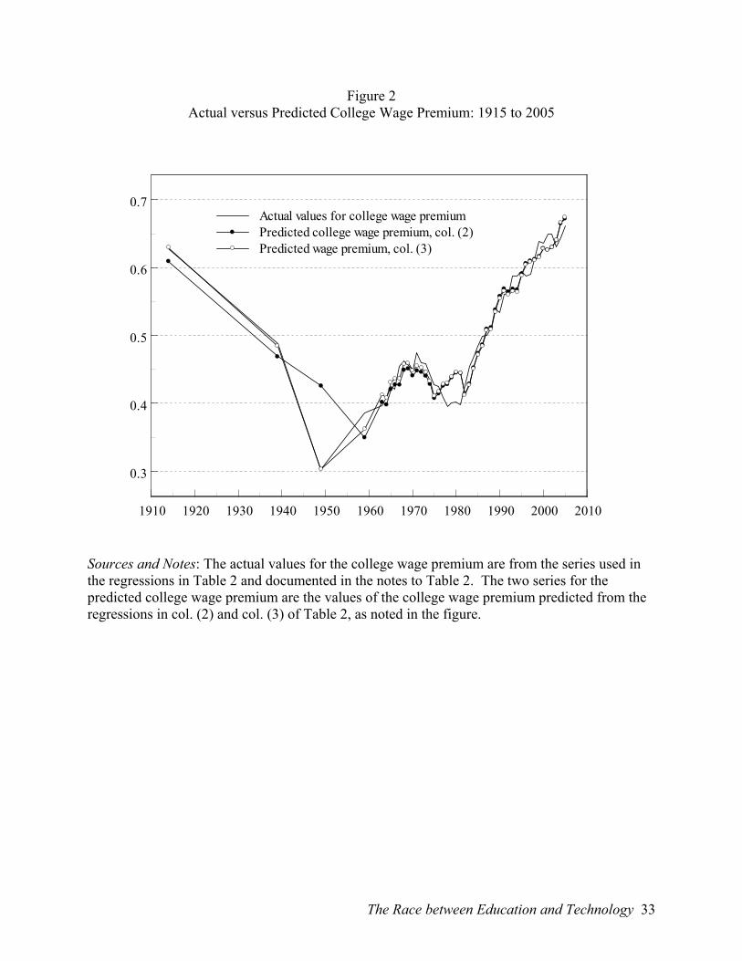
Figure 2 Actual versus Predicted College Wage Premium: 1915 to 2005

1910 1920 1930 1940 1950 1960 1970 1980 1990 2000 2010

0.3

0.4

0.5

0.6

0.7Actual values for college wage premiumPredicted college wage premium, col. (2)Predicted wage premium, col. (3)

Sources and Notes: The actual values for the college wage premium are from the series used in the regressions in Table 2 and documented in the notes to Table 2. The two series for the predicted college wage premium are the values of the college wage premium predicted from the regressions in col. (2) and col. (3) of Table 2, as noted in the figure.


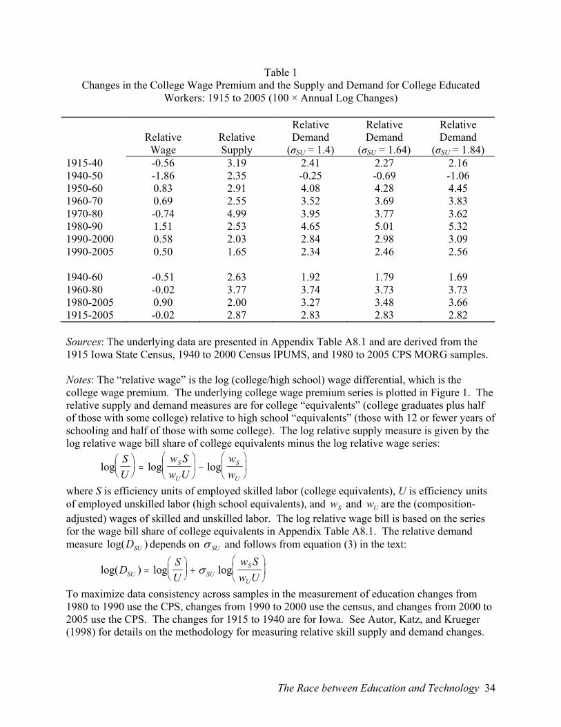
Table 1 Changes in the College Wage Premium and the Supply and Demand for College Educated

Workers: 1915 to 2005 (100 × Annual Log Changes)

Relative Wage

Relative Supply

Relative Demand

(σSU = 1.4)

Relative Demand

(σSU = 1.64)

Relative Demand

(σSU = 1.84) 1915-40 -0.56 3.19 2.41 2.27 2.16 1940-50 -1.86 2.35 -0.25 -0.69 -1.06 1950-60 0.83 2.91 4.08 4.28 4.45 1960-70 0.69 2.55 3.52 3.69 3.83 1970-80 -0.74 4.99 3.95 3.77 3.62 1980-90 1.51 2.53 4.65 5.01 5.32 1990-2000 0.58 2.03 2.84 2.98 3.09 1990-2005 0.50 1.65 2.34 2.46 2.56 1940-60 -0.51 2.63 1.92 1.79 1.69 1960-80 -0.02 3.77 3.74 3.73 3.73 1980-2005 0.90 2.00 3.27 3.48 3.66 1915-2005 -0.02 2.87 2.83 2.83 2.82 Sources: The underlying data are presented in Appendix Table A8.1 and are derived from the 1915 Iowa State Census, 1940 to 2000 Census IPUMS, and 1980 to 2005 CPS MORG samples. Notes: The “relative wage” is the log (college/high school) wage differential, which is the college wage premium. The underlying college wage premium series is plotted in Figure 1. The relative supply and demand measures are for college “equivalents” (college graduates plus half of those with some college) relative to high school “equivalents” (those with 12 or fewer years of schooling and half of those with some college). The log relative supply measure is given by the log relative wage bill share of college equivalents minus the log relative wage series:

log log logSU

w Sw U

ww

S

U

S

U

⎛⎝⎜

⎞⎠⎟ =

⎛⎝⎜

⎞⎠⎟ −

⎛⎝⎜

⎞⎠⎟

where S is efficiency units of employed skilled labor (college equivalents), U is efficiency units of employed unskilled labor (high school equivalents), and and are the (composition-adjusted) wages of skilled and unskilled labor. The log relative wage bill is based on the series for the wage bill share of college equivalents in Appendix Table A8.1. The relative demand measure depends on

wS wU

log( )DSU σ SU and follows from equation (3) in the text:

log( ) log logDSU

w Sw USU SU

S

U=

⎛⎝⎜

⎞⎠⎟ +

⎛⎝⎜

⎞⎠⎟σ

To maximize data consistency across samples in the measurement of education changes from 1980 to 1990 use the CPS, changes from 1990 to 2000 use the census, and changes from 2000 to 2005 use the CPS. The changes for 1915 to 1940 are for Iowa. See Autor, Katz, and Krueger (1998) for details on the methodology for measuring relative skill supply and demand changes.


Table 2 Determinants of the College Wage Premium: 1915 to 2005

(1) (2) (3) (4) (5) (College/high school) supply -0.544

(0.079) -0.595 (0.093)

-0.610 (0.065)

-0.579 (0.099)

-0.618 (0.079)

(College/high school) supply × post-1949

0.0078 (0.0420)

Time 0.00378 (0.00200)

0.00970 (0.00243)

0.00991 (0.00171)

0.00973 (0.00545)

0.0103 (0.0028)

Time × post-1949 0.0188 (0.0013)

Time × post-1959 0.0156 (0.0012)

0.0154 (0.0009)

0.0150 (0.0022)

Time × post-1992 -0.00465 (0.00227)

-0.00807 (0.00279)

-0.00739 (0.00196)

-0.00742 (0.00199)

1949 Dummy -0.137 (0.021)

-0.143 (0.036)

Time2 × 10 -0.00342 (0.00203)

Time3 × 1000 0.105 (0.034)

Time4 × 10,000 0.00664 (0.00186)

Constant -0.493 (0.168)

-0.645 (0.197)

-0.656 (0.138)

-0.587 (0.210)

-0.674 (0.079)

R2 0.934 0.917 0.960 0.928 0.960 Number of observations 47 47 47 47 47 Sources and Notes: Each column is an OLS regression of the college wage premium on the indicated variables using a sample covering the years 1914, 1939, 1949, 1959, and 1963 to 2005. Standard errors are given in parentheses below the coefficients. The college wage premium is a fixed weighted average of the estimated college (exactly 16 years of schooling) and post-college (17+ years of schooling) wage differential relative to high school graduates (those with exactly 12 years of schooling). (College/high school) supply is the log supply of college equivalents to high school equivalents both measured in efficiency units. The data for 1963 to 2005 are from the 1964 to 2006 March CPS samples. The college wage premium and relative supplies in efficiency units for 1963 to 2005 use the same data processing steps and sample selection rules as those described in the data appendix to Autor, Katz, and Kearney (2007). The college wage premium for 1963 to 2005 uses the log weekly earnings of full-time, full-year workers. The college wage premium observations for 1914, 1939, 1949, and 1959 append the changes in the college wage premium series from 1915 to 1970 (actually 1914 to 1969) plotted in Figure 1 to the 1969 data point from our March CPS series. The log relative supply observations for 1914 to 1959 similarly append changes in the relative supply of college equivalents from 1914 to 1939 for Iowa and for the United States from 1939 to 1949, 1949 to 1959, and 1959 to 1969 from the Census IPUMS samples using the efficiency-units measurement approach of Tables 5 and 6.


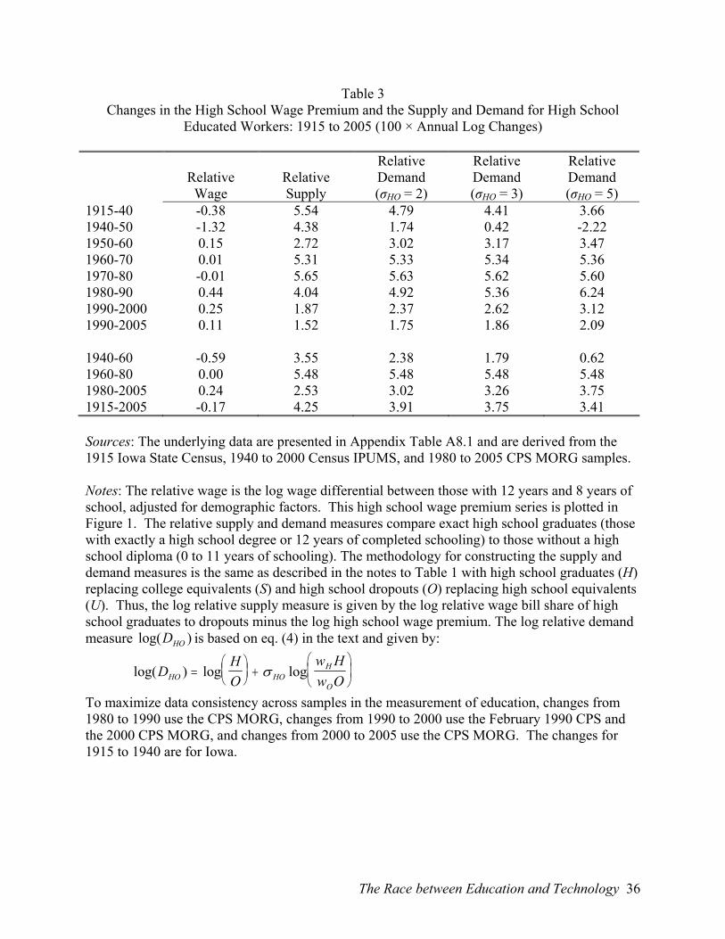
Table 3 Changes in the High School Wage Premium and the Supply and Demand for High School

Educated Workers: 1915 to 2005 (100 × Annual Log Changes)

Relative Wage

Relative Supply

Relative Demand (σHO = 2)



1915-40 -0.38 5.54 4.79 4.41 3.66 1940-50 -1.32 4.38 1.74 0.42 -2.22 1950-60 0.15 2.72 3.02 3.17 3.47 1960-70 0.01 5.31 5.33 5.34 5.36 1970-80 -0.01 5.65 5.63 5.62 5.60 1980-90 0.44 4.04 4.92 5.36 6.24 1990-2000 0.25 1.87 2.37 2.62 3.12 1990-2005 0.11 1.52 1.75 1.86 2.09 1940-60 -0.59 3.55 2.38 1.79 0.62 1960-80 0.00 5.48 5.48 5.48 5.48 1980-2005 0.24 2.53 3.02 3.26 3.75 1915-2005 -0.17 4.25 3.91 3.75 3.41 Sources: The underlying data are presented in Appendix Table A8.1 and are derived from the 1915 Iowa State Census, 1940 to 2000 Census IPUMS, and 1980 to 2005 CPS MORG samples. Notes: The relative wage is the log wage differential between those with 12 years and 8 years of school, adjusted for demographic factors. This high school wage premium series is plotted in Figure 1. The relative supply and demand measures compare exact high school graduates (those with exactly a high school degree or 12 years of completed schooling) to those without a high school diploma (0 to 11 years of schooling). The methodology for constructing the supply and demand measures is the same as described in the notes to Table 1 with high school graduates (H) replacing college equivalents (S) and high school dropouts (O) replacing high school equivalents (U). Thus, the log relative supply measure is given by the log relative wage bill share of high school graduates to dropouts minus the log high school wage premium. The log relative demand measure is based on eq. (4) in the text and given by: log( )DHO

log( ) log logDHO

w Hw OHO HO

H

O=

⎛⎝⎜

⎞⎠⎟ +

⎛⎝⎜

⎞⎠⎟σ

To maximize data consistency across samples in the measurement of education, changes from 1980 to 1990 use the CPS MORG, changes from 1990 to 2000 use the February 1990 CPS and the 2000 CPS MORG, and changes from 2000 to 2005 use the CPS MORG. The changes for 1915 to 1940 are for Iowa.


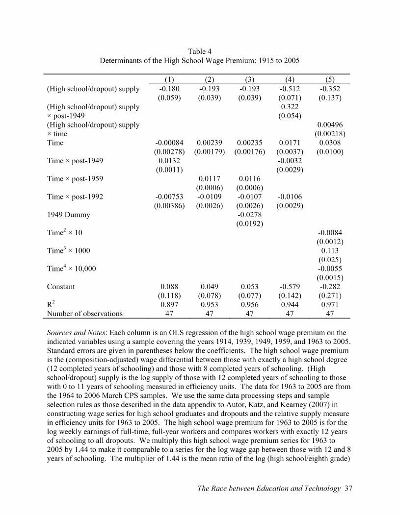
Table 4 Determinants of the High School Wage Premium: 1915 to 2005

(1) (2) (3) (4) (5) (High school/dropout) supply -0.180

(0.059) -0.193 (0.039)

-0.193 (0.039)

-0.512 (0.071)

-0.352 (0.137)

(High school/dropout) supply × post-1949

0.322 (0.054)

(High school/dropout) supply × time

0.00496 (0.00218)

Time -0.00084 (0.00278)

0.00239 (0.00179)

0.00235 (0.00176)

0.0171 (0.0037)

0.0308 (0.0100)

Time × post-1949 0.0132 (0.0011)

-0.0032 (0.0029)

Time × post-1959 0.0117 (0.0006)

0.0116 (0.0006)

Time × post-1992 -0.00753 (0.00386)

-0.0109 (0.0026)

-0.0107 (0.0026)

-0.0106 (0.0029)

1949 Dummy -0.0278 (0.0192)

Time2 × 10 -0.0084 (0.0012)

Time3 × 1000 0.113 (0.025)

Time4 × 10,000 -0.0055 (0.0015)

Constant 0.088 (0.118)

0.049 (0.078)

0.053 (0.077)

-0.579 (0.142)

-0.282 (0.271)

R2 0.897 0.953 0.956 0.944 0.971 Number of observations 47 47 47 47 47 Sources and Notes: Each column is an OLS regression of the high school wage premium on the indicated variables using a sample covering the years 1914, 1939, 1949, 1959, and 1963 to 2005. Standard errors are given in parentheses below the coefficients. The high school wage premium is the (composition-adjusted) wage differential between those with exactly a high school degree (12 completed years of schooling) and those with 8 completed years of schooling. (High school/dropout) supply is the log supply of those with 12 completed years of schooling to those with 0 to 11 years of schooling measured in efficiency units. The data for 1963 to 2005 are from the 1964 to 2006 March CPS samples. We use the same data processing steps and sample selection rules as those described in the data appendix to Autor, Katz, and Kearney (2007) in constructing wage series for high school graduates and dropouts and the relative supply measure in efficiency units for 1963 to 2005. The high school wage premium for 1963 to 2005 is for the log weekly earnings of full-time, full-year workers and compares workers with exactly 12 years of schooling to all dropouts. We multiply this high school wage premium series for 1963 to 2005 by 1.44 to make it comparable to a series for the log wage gap between those with 12 and 8 years of schooling. The multiplier of 1.44 is the mean ratio of the log (high school/eighth grade)


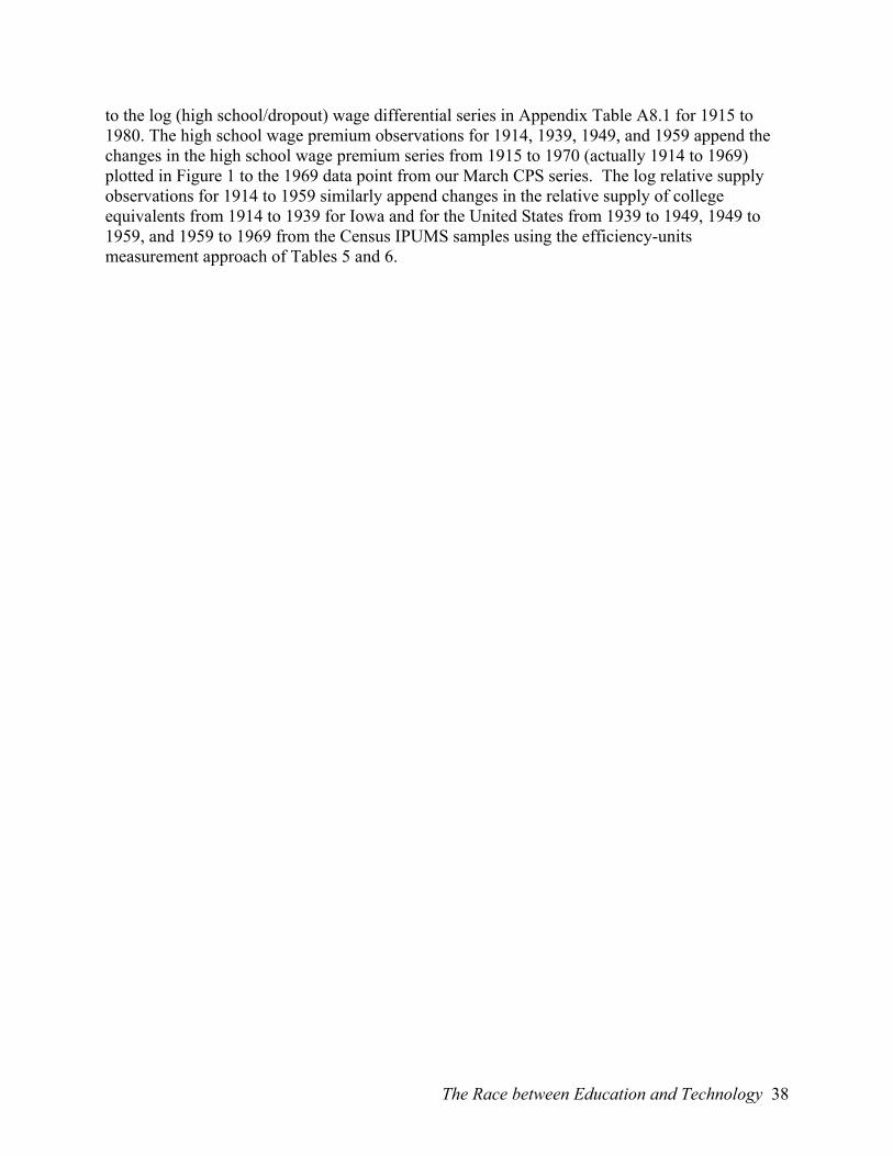
to the log (high school/dropout) wage differential series in Appendix Table A8.1 for 1915 to 1980. The high school wage premium observations for 1914, 1939, 1949, and 1959 append the changes in the high school wage premium series from 1915 to 1970 (actually 1914 to 1969) plotted in Figure 1 to the 1969 data point from our March CPS series. The log relative supply observations for 1914 to 1959 similarly append changes in the relative supply of college equivalents from 1914 to 1939 for Iowa and for the United States from 1939 to 1949, 1949 to 1959, and 1959 to 1969 from the Census IPUMS samples using the efficiency-units measurement approach of Tables 5 and 6.


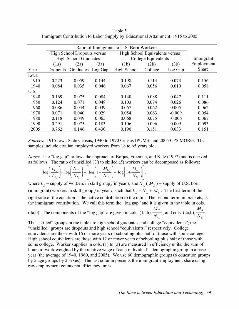
Table 5 Immigrant Contribution to Labor Supply by Educational Attainment: 1915 to 2005

Ratio of Immigrants to U.S. Born Workers High School Dropouts versus

High School Graduates High School Equivalents versus

College Equivalents

(1a) (2a) (3a) (1b) (2b) (3b) Year Dropouts Graduates Log Gap High School College Log Gap

Immigrant Employment

Share Iowa 1915 0.223 0.059 0.144 0.198 0.114 0.073 0.156 1940 0.084 0.035 0.046 0.067 0.056 0.010 0.058 U.S. 1940 0.169 0.075 0.084 0.140 0.088 0.047 0.111 1950 0.124 0.071 0.048 0.103 0.074 0.026 0.086 1960 0.086 0.044 0.039 0.067 0.062 0.005 0.062 1970 0.071 0.040 0.029 0.054 0.063 -0.009 0.054 1980 0.118 0.049 0.065 0.068 0.075 -0.006 0.067 1990 0.291 0.075 0.183 0.106 0.096 0.009 0.093 2005 0.762 0.146 0.430 0.190 0.151 0.033 0.151 Sources: 1915 Iowa State Census, 1940 to 1990 Census IPUMS, and 2005 CPS MORG. The samples include civilian employed workers from 18 to 65 years old. Notes: The “log gap” follows the approach of Borjas, Freeman, and Katz (1997) and is derived as follows. The ratio of unskilled (U) to skilled (S) workers can be decomposed as follows:

log log log logLL

NN

MN

MN

U

S

U

S

U

U

S

S

t

t

t

t

t

t

t

t

⎛

⎝⎜⎜

⎞

⎠⎟⎟ =

⎛

⎝⎜⎜

⎞

⎠⎟⎟ + +

⎛

⎝⎜⎜

⎞

⎠⎟⎟ − +

⎛

⎝⎜⎜

⎞

⎠⎟⎟

⎡

⎣⎢⎢

⎤

⎦⎥⎥

1 1 ,

where = supply of workers in skill group j in year t, and ( ) = supply of U.S. born (immigrant) workers in skill group j in year t, such that

LjtN jt

M jt

L N Mj jt t jt= + . The first term of the

right side of the equation is the native contribution to the ratio. The second term, in brackets, is the immigrant contribution. We call this term the “log gap” and it is given in the table in cols.

(3a,b). The components of the “log gap” are given in cols. (1a,b),MN

U

U

t

t

, and cols. (2a,b),MN

S

S

t

t

.

The “skilled” groups in the table are high school graduates and college “equivalents”; the “unskilled” groups are dropouts and high school “equivalents,” respectively. College equivalents are those with 16 or more years of schooling plus half of those with some college. High school equivalents are those with 12 or fewer years of schooling plus half of those with some college. Worker supplies in cols. (1) to (3) are measured in efficiency units: the sum of hours of work weighted by the relative wage of each individual’s demographic group in a base year (the average of 1940, 1960, and 2005). We use 60 demographic groups (6 education groups by 5 age groups by 2 sexes). The last column presents the immigrant employment share using raw employment counts not efficiency units.


Table 6 Contribution of Immigrants and the U.S. Native-Born to the Growth of Relative Skill Supplies:

1915 to 2005 (100 × Annual Log Changes)

High School Graduates/ High School Dropouts

College Equivalents/ High School Equivalents

Period Total Immigrant Native-Born Total Immigrant Native-Born1915-40 4.80 0.39 4.41 2.82 0.25 2.57 1940-60 3.49 0.22 3.26 2.96 0.21 2.75 1960-80 5.61 -0.13 5.74 3.89 0.06 3.83 1980-2005 2.49 -1.46 3.95 2.27 -0.16 2.43 Sources: See Table 5. Notes: Each cell in the table is the annualized percentage change, from the beginning to the end of the period, of relative skill supplies measured in efficiency units. The total column gives the overall growth in relative skill supply. The immigrant and native-born columns decompose the overall relative skill supply growth into the immigrant and native contributions defined in the notes to Table 5. The immigrant column can be computed from the data in Table 5 cols. (3a.b) “log gap,” which is the immigrant contribution to the relative skill supply. For example, from 1980 to 2005 the “log gap” for high school dropouts versus high school graduates went from 0.065 to 0.430 (Table 5, col. 3a). If there had been no foreign born in 1980, the log ratio of high school graduates to dropouts would have increased by 6.5 log points and in 2005 it would have increased by 43 log points. Thus, the annualized contribution of immigrants to changes in log(H/O) from 1980 to 2005 is given by [(0.065 – 0.430) × 100/25] = –1.46. See the notes to Table 5 for the definitions of college and high-school equivalents and efficiency units.


Table 7 High School Graduates as a Share of the Labor Force (≥ 14 years old)

Administrative Records

(1) Census

(2) Year 1890 0.040 0.063 1900 0.044 0.080 1910 0.054 0.102 1920 0.079 0.150 1930 0.123 0.212 Change in high school graduate share 1890 to 1910 0.014 0.039 1910 to 1930 0.069 0.110 Change in log relative supply 1890 to 1910 0.315 0.523 1910 to 1930 0.899 0.857 Annualized log relative supply change × 100 1890 to 1910 1.57 2.62 1910 to 1930 4.49 4.28 Sources: The estimates in col. (1) are from Goldin and Katz (1995, table 8). The estimates in col. (2) use the 1915 Iowa State Census and the 1880 to 1940 Census IPUMS. Notes: The relative supply measure is the ratio of high school graduates to those with less than 12 years of schooling. The col. (1) estimates use the administrative data on flows of new high school graduates from Figure 1, Chapter 6 to build up stocks of high school graduates following the methodology described in the notes to table 8 of Goldin and Katz (1995). The col. (2) estimates use individual-level data on all labor force participants (those reporting a gainful occupation) aged 14 years or older in each Census IPUMS from 1880 to 1930. We impute the probability that a labor force participant in the 1880 to 1930 Census IPUMS is a high school graduate based on high school graduate shares by birth cohort and sex in the 1915 Iowa State Census (for pre-1890 birth cohorts) and the 1940 Census IPUMS (for 1890 to 1916 birth cohorts). The Iowa estimates for pre-1890 birth cohorts are multiplied by 0.8, the mean ratio of the high graduate share for the overall U.S. to Iowa residents for 1870 to 1890 birth cohorts in the 1940 IPUMS. We assume that labor force participation rate from 1880 to 1930 was the same for male high school graduates and less-educated males. We assume that the labor force participation rate of adult female high school graduates (those 21 years and older) was 1.4 times the rate of less-educated adult females for 1880 to 1930. These assumptions are based on the labor force participation rates by education, sex, and cohort in the 1915 Iowa sample and 1940 IPUMS. We adjust downward the high school graduation rates of those 14 to 19 years old to reflect the lower labor force participation rates of those continuing in school. The 1890 estimate of the high school graduate labor force share is the average of the 1880 and 1900 estimates since there is no 1890 Census IPUMS sample.


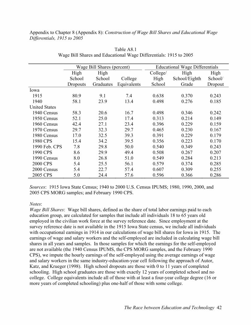
Appendix to Chapter 8 (Appendix 8): Construction of Wage Bill Shares and Educational Wage Differentials, 1915 to 2005

Table A8.1 Wage Bill Shares and Educational Wage Differentials: 1915 to 2005

Wage Bill Shares (percent) Educational Wage Differentials High

School Dropouts

High School

Graduates

College

Equivalents

College/ High

School

High School/Eighth

Grade

High School/ Dropout

Iowa 1915 80.9 9.1 7.4 0.638 0.370 0.243 1940 58.1 23.9 13.4 0.498 0.276 0.185 United States 1940 Census 58.3 20.6 16.7 0.498 0.346 0.242 1950 Census 52.1 25.0 17.4 0.313 0.214 0.149 1960 Census 42.4 27.1 23.4 0.396 0.229 0.159 1970 Census 29.7 32.3 29.7 0.465 0.230 0.167 1980 Census 17.0 32.5 39.3 0.391 0.229 0.179 1980 CPS 15.4 34.2 39.5 0.356 0.223 0.170 1990 Feb. CPS 7.8 29.8 50.0 0.540 0.349 0.243 1990 CPS 8.6 29.9 49.4 0.508 0.267 0.207 1990 Census 8.0 26.8 51.0 0.549 0.284 0.213 2000 CPS 5.4 25.5 56.1 0.579 0.374 0.285 2000 Census 5.4 22.7 57.4 0.607 0.309 0.255 2005 CPS 5.0 24.4 57.6 0.596 0.366 0.286 Sources: 1915 Iowa State Census; 1940 to 2000 U.S. Census IPUMS; 1980, 1990, 2000, and 2005 CPS MORG samples; and February 1990 CPS. Notes: Wage Bill Shares: Wage bill shares, defined as the share of total labor earnings paid to each education group, are calculated for samples that include all individuals 18 to 65 years old employed in the civilian work force at the survey reference date. Since employment at the survey reference date is not available in the 1915 Iowa State census, we include all individuals with occupational earnings in 1914 in our calculations of wage bill shares for Iowa in 1915. The earnings of wage and salary workers and the self-employed are included in calculating wage bill shares in all years and samples. In those samples for which the earnings for the self-employed are not available (the 1940 Census IPUMS, the CPS MORG samples, and the February 1990 CPS), we impute the hourly earnings of the self-employed using the average earnings of wage and salary workers in the same industry-education-year cell following the approach of Autor, Katz, and Krueger (1998). High school dropouts are those with 0 to 11 years of completed schooling. High school graduates are those with exactly 12 years of completed school and no college. College equivalents include all of those with at least a four-year college degree (16 or more years of completed schooling) plus one-half of those with some college.


Educational Wage Differentials: The log college/high school wage differential is a weighted average of the estimated college (exactly 16 years of completed schooling or bachelor’s degree) and post-college (17+ years of schooling or a post-baccalaureate degree) wage premium relative to high school graduates (those with exactly 12 years of completed schooling or a high school diploma) for the year given. The weights are the employment shares of college and post-college workers in 1980. The log (high school/eighth grade) wage differential is the estimated wage premium for those with exactly a high school degree (12 years of completed schooling) and those with exactly 8 years of completed schooling. Changes in education coding in the census and CPS lead us to include workers with 5 to 8 years of completed schooling in the eighth grade category for the 1990 and 2000 Census, February 1990 CPS, and the 2000 and 2005 CPS MORG samples. The log (high school/dropout) wage differential is a weighted average of the estimated wage premium for those with exactly a high school degree (12 years of completed schooling) relative to 4 groups of “dropouts,” those with exactly 8, 9, 10, and 11 years of completed schooling. The weights are the employment shares in 1980 of dropouts with 8, 9, 10, and 11 years of completed schooling. Educational wage differentials for the United States for 1940 to 2005 are estimated in each sample using a standard cross-section regression of log hourly earnings on dummies for single years of schooling (or degree attainment) categories (some schooling categories contain multiple years with education coding changes in 1990), a quartic in experience, three region dummies, a part-time dummy, a female dummy, a nonwhite dummy, and interaction terms between the female dummy and quartic in potential experience and the nonwhite dummy. The educational wage differentials are directly taken from the coefficients on the dummy variables for schooling categories. The regression samples include civilian employees from 18 to 65 years old. The regression specification and the specific data processing steps follow the approach of Autor, Katz, and Krueger (1998, table 1). Estimates of educational wage differentials for Iowa from 1915 to 1940 required a different treatment based on our concerns with the meaning of college education for older cohorts in the 1915 Iowa state census, and difficulties in measuring the returns to education for women in the early twentieth century given the potential importance of unpaid family work. These issues are discussed in detail in Goldin and Katz (2000). We use our preferred estimates of the returns to a year of college for young men (18 to 34 years olds) in 1914 and 1939 from Chapter 2, Table 7 to estimate the change in the log college high school wage differential from 1915 to 1940. The return to a year of schooling for young men decreased by 0.033, from 0.148 in 1915 to 0.115 in 1940, which implies a decline in the log (college/high school) wage differential of 0.140 from 1915 to 1940 after proportionally scaling up the 1940 return to a year of college for young men by a factor of 4.307 to equal the 1940 national (college/high school) wage differential of 0.498 for all workers aged 18 to 65 years. The log (high school/eighth grade) and (high school/dropout) wage differentials for Iowa in 1915 and 1940 are estimated from samples of non-farm, full-year male civilian workers aged 18 to 65


years in the 1915 Iowa State Census and from those residing in Iowa in the 1940 Census IPUMS. These measures of the high school wage premium are taken from cross-section regressions of log annual earnings on dummy variables for single year of schooling categories, a quartic in potential experience, and dummy variables for nonwhites and for foreign born status. Hours and weeks of work are not available in the 1915 Iowa State Census but information on months of unemployment in 1914 is available. Full-year workers for 1915 are those with earnings in 1914 but no unemployment in 1914. Full-year workers in 1940 are those who worked at least 50 weeks in 1939.


the race between education and technology: the … · the race between education and technology:...

Documents