the real chinese gross domestic product (gdp)

Review of Income and Wealth Series 39, Number 1, March 1993

THE "REAL" CHINESE GROSS DOMESTIC PRODUCT (GDP)

FOR THE PRE-REFORM PERIOD 1952-77

The University of Adelaide

This paper develops an econometric method based on the relationship between GDP and NMP to estimate an unknown Chinese GDP series of 1952-77 using recently available Chinese GDP data of 1978-90 and a reconstructed NMP series of 1952-90. In this manner, a long-term (1952-90) series of China's GDP has been obtained for long-term analyses. A reassessment of Chinese economic performance of 1952-90 using this series suggests that the paper's estimate provides a reasonable reflection of both the Chinese pre-and post-reform economic growth in terms of production structure, growth pattern and policy changes. A series of China's per capita GDP in U.S. dollars which is comparable to the World Bank's estimate for the early 1980s has also been obtained.

This paper has two main objectives. First, a long-term series of China's Gross Domestic Product (GDP) will be created. Second, this series will be used to reassess Chinese economic performance in the period 1952-90.

Economic reforms have brought about a rapid economic growth and structural change in China since 1978. There has been a growing interest in the performance of Chinese economy in the current transition from a typical central planning to a market-oriented economy. Therefore, there has been a need for a reliable long-term data on China's national product to assess this performance. Until 1988, however, China had never measured its national product in the western way, that is, its national product differs from the System of National Accounts (SNA) concept of GDP (UN 1968).' China's national product had only been measured by the Material Product System (MPS) as Net Material Product (NMP). Since NMP differs significantly from GDP, it can be very misleading to assess Chinese economic growth (which western economists nor- mally identify as the growth of GDP) using China's NMP data.' In 1987, to facilitate the process of economic reforms, the Chinese government decided to establish China's first SNA input-output table and started estimating GDP, while retaining the old MPS. In 1988 China's State Statistical Bureau (CSSB) started

Note: I am most grateful to Tin Nguyen and Christopher Findlay for very helpful discussions. Thanks also go to Andrew Watson, Ian McLean, Yanrui Wu and two anonymous referees of the journal for comments on the earlier drafts. The work reported in this paper was supported by grants from the Australian Research Council and the University of Adelaide University Research Grants Scheme. I alone am responsible for any errors contained in this study.

'See also Ruggles and Ruggles (1970) for the details of SNA. '~stimation of Chinese GDP, especially for the period of the 1960s-1970s, was dependent upon

work by western scholars, for example, Li (1959), Liu and Yeh (1965), Rawski (1980), Perkins (1980) and Field (1980). However, estimation of GDP was extremely difficult during the 1960s and 1970s when even NMP data were not openly published.

to issue GDP for China. The estimate of 1978-87 GDP has also been made by the CSSB (CSSB, 19883, p. 36). Nevertheless, for many studies involving long-term analyses, the available Chinese GDP series is too short. In particular, to compare the economic growth in post-reform with that of pre-reform period, an estimate of Chinese GDP for the period of pre-1978 is required. By using the econometric method, this paper attempts to estimate China's GDP for 1952-77 so that a GDP series of a longer period (1952-90) can be obtained. By using such a GDP series, this paper also attempts to reassess Chinese economic performance in both pre- and post-reform periods in terms of the changes in production structure, growth patterns and per capita GDP.

In Section 2, after a simple review of the relationship between GDP and NMP, the methodology used in this paper is discussed. The relevant data problems are discussed in Section 3. The estimation of Chinese GDP for the period 1952-77 and a reassessment of Chinese economic performance for the period 1952-90 is given in Sections 4 and 5. A summary of conclusions is presented in Section 6.

2.1. The Relationship between GDP and NMP

The MPS follows the Marxian concept of "productive" and "non-productive" economic activities. Only those activities producing physical or material products are regarded "productive." The "material production" is composed of five sectors: agriculture, industry, construction, transportation and c~mmerce .~ Those activities producing services or "non-material products" are, however, regarded "non-productive" (Li ed. 1986, pp. 618-619). Value added by most services is therefore excluded from the calculation of national p r ~ d u c t . ~

Since the MPS emphasizes "material production," Chinese official statisticians are first interested in the total value of physical goods. It includes not only newly added value but also the transferred value, that is, the value of factors consumed in the process of production.5 This is called Gross Output Value or GOV. For each sector i, let the value of material input be C" the value of depreciation be and the newly added value by "material production" be v ? , ~ GOV, can be denoted as

Thus, for the economy as a whole, we have

(2) GOV = X i GOVi = Zi (C" C: + Vm).

3 ~ e r e agriculture includes farming, forestry, husbandry, sidelines and fishery; industry includes mining and manufacturing; transportation only includes the so-called "material productionw-linked transportation, post and telecommunication; and commerce includes catering trade and "material productionM-linked conpnerce and storage trade (Li, ed., 1986, pp. 607-608).

4See Table A-1 for the details of the services excluded from NMP. ' ~ n Capital, Marx writes: "The values of the annual product in commodities.. .resolves itself

into two parts: Part A, which replaces the value of the advanced constant capital, and Part B, which represents itself in the form of wages, profit, and rent." (Capital, Vol. 3, p. 377, Charles H. Kerr & Co., Chicago, 1909.)

6 V y is also referred to by the Chinese statisticians as Net Output Value (NOV).

It is clear that there is some double counting in GOV, because it includes all intermediate inputs (EiCr) . Thus, the net material product, NMP, can be written as

(3) NMP = ZiNMPi = ZiVT.

Now, for each sector, i let GDP, be defined as

where V; stands for the value added by "non-material production" for each sector i. For the economy as a whole, we have

where Z is the sum of the value of depreciation and the value added by "non-material production," X,(C:+ V;). Z can be estimated using available GDP and NMP series.

2.2. Estimated Model

We now further discuss the relationship between GDP, and NMP,. From the previous discussions, it is obvious that GDP, can be expressed as a function of NMP, (or Xi for convenience) and an error term u,, i.e.

Let us assume that

By definition, Z, is the sum of the value of capital consumption, c:, and the value added by the so-called "non-material services," V?. Usually, C : much smaller and more stable than V?, so that 2, largely represents V;. Since services are generally considered as "luxury goods," the share of Z, in GDP, will be expected to increase as GDP, increases. This is often observed in many countries and appears to be theoretically justified according to Engel's Law.

Now from equation (8) with ui = E(u,) = 0, the share of Zi in GDP, can be defined as

'TO be sure, for the industrial and agricultural sectors, Z,/GDP, can be negligible. Note that, for the economy as a whole, the share of Z in GDP is

This suggests that, provided that the share of the service sector in total output increases over time, Z/GDP can increase over time as GDP increases, even if Z,/GDP, remains constant for each sector. This is because the service sector has a larger share than the other two sectors.

Obviously, as Xi (i.e. NMP,) increases, Z,/GDP, will increase only if b <O. By taking the logarithm of both sides of equation (8) we have

where a, =In B,. Equation (10) can be estimated by using OLS regression and can then be used to generate estimates for GDP, of the period 1952-77, given values for X, (i.e. NMP,) in this period. From the estimate of GDP, for each sector i, the GDP for the economy as a whole can be obtained as follows,

3. DATA

3.1. Data Availability

In recently published CSSB yearbooks both GDP and NMP data series are reported as aggregate figures for the whole economy and with a sectoral break- down. At the sectoral level, the GDP is available as agriculture (A), industry ( I ) and services (S), r e s p e c t i ~ e l ~ . ~ The NMP data for each sector are available in terms of the five material sectors of agriculture (AG), mining and manufacturing (MM), construction (CS), transportation (TR) and commerce (CM). The data series are from 1978 to 1990 for GDP and from 1952 to 1990 for NMP. Both are available in value terms at current prices and as indices (1978 = 100 for GDP

TABLE 1

CHINESE GDP AT CURRENT A N D 1980 PRICES, TOTAL A N D BY SECTOR, 1978-90

(in billion Rmb yuan)

Current Prices 1980 Prices

Year GDP GDP, GDP, GDP, GDP GDP, GDP, GDP,

Source: Data at current prices are from CSSB, 1991, p. 31. Data at 1980 prices are this author's estimates based on official GDP indices (1952 = 100) (from the same source) and the 1980 GDP value for each sector.

Note: A = Agriculture; I = Industry; S = Services.

'GDPT = elnGDP:, where in GDPP = aT + b: In X, (a : and b: are OLS fitted values of a, and b;). '1n fact, CSSB uses the terms primary, secondary and tertiary to name the three sectors, but

their meanings are similar to those of U N classificiation of the A, I and S sectors. Here A, I and S are used in order to be consistent with the U N classification.

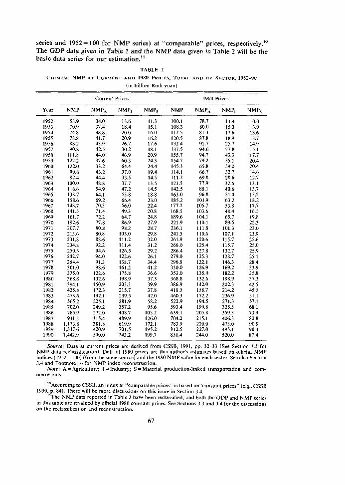
series and 1952= 100 for NMP series) at "comparable" prices, respectively.10 The GDP data given in Table 1 and the NMP data given in Table 2 will be the basic data series for our estimation."

TABLE 2

CHINESE NMP AT CURRENT AND 1980 PRICES, TOTAL AND BY SECTOR, 1952-90 (in billion Rmb yuan)


Year NMP NMP,, NMP, NMP, NMP NMP, NMP, NMP,

Source: Data at current prices are derived from CSSB, 1991, pp. 32-33 (See Section 3.3 for NMP data reclassification). Data at 1980 prices are this author's estimates based on official NMP indices (1952 = 100) (from the same source) and the 1980 NMPvalue for each sector. See also Section 3.4 and Footnote 16 for NMP index reconstruction.

Note: A = Agriculture; I = Industry; S = Material production-linked transportation and commerce only.

'O~ccording to CSSB, an index at "comparable prices" is based on"constant prices" (e.g., CSSB 1990, p. 84). There will be more discussions on this issue in Section 3.4.

"The NMP data reported in Table 2 have been reclassified, and both the GDP and NMP series in this table are revalued by official 1980 constant prices. See Sections 3.3 and 3.4 for the discussions on the reclassification and reconstruction.

67

3.2. The Quality of China's Oficial GDP of 1978-90

The extrapolation of China's 1952-77 GDP must be based on a reliable GDP series for the current period (1978-90). At present, both CSSB and the World Bank are issuing GDP estimates for China. The World Bank's estimation began earlier than the CSSB's. In 1984, based on newly released NMP data, a team of World Bank experts were able to establish the first SNA input-output model to estimate China's 1981 G D P (World Bank, 1985, p. 4). Nevertheless, because of "assumptions and guess-work" as well as "rough adjustment," owing to incom- plete data and, especially, the lack of data for intersectoral flows and for the so-called "non-material production sector," the quality of the World Bank estimate has remained in question.

Perhaps encouraged by the World Bank, in 1985 the Chinese State Council approved a CSSB report establishing the statistics for the tertiary sector, including "non-material production." This was a major step towards adopting the SNA (CSSB, 1985a, pp. 120-124). In 1987, the Chinese government decided to establish China's first SNA input-output table and started estimating GDP (CSSB, 1988a, pp. 311-312 and 481-482).12 As the CSSB's Input-Output Office (100 ) reported, the compiling of China's 1987 Input-Output Table, including 120 industries and government departments, of which 104 were "material" and 16 were "non- material," started with overall investigations and sample surveys at both enterprise and household levels for each province and municipality throughout 1988 (100 , 1987, p. 30). Meanwhile, more comprehensive experiments were carried out in nine provinces and municipalities to change the old (NMP) accounting system to meet the requirements of SNA, and adjust available historical accounting materials so that GDP can be estimated (AODSM, 1989, pp. 26-27). Since the major principles of SNA have been followed and all the unpublished data are available, it is expected that the GDP figures currently issued by CSSB are closer to reality than the World Bank estimates.13

3.3. Sectoral Reclassijication of NMP

When the World Bank was making its estimate for China's 1981 GDP in 1984, one of the major difficulties was that the available Chinese statistics included rural production brigade- and team-run industrial enterprises as part of the agricultural sector (World Bank, 1985, p. 3).14 This problem has now been solved. Following a decision made by CSSB at the end of 1984 (Li, ed., 1986, pp. 115-119), the output of the rural industrial sector is counted in the output of the industrial sector as a whole from 1985 onwards (CSSB, 1985b, pp. 244-249). The NMP

I2 In fact, China started input-output study in the mid-1960s and designed its first MPS input- output table (1973 Table) in 1974-76. In addition, another two MPS input-output tables (1981 and 1983 Tables) were constructed and used in 1982 and 1984 by CSSB and the State Planning Committee (Li, 1987, pp. 30-31). However, this information has not yet been officially reported.

"Although there are still some problems to solve before completely meeting the criteria of SNA, the Chinese 1987 Input-Output Table was accepted by the international experts in the 9th International Conference of Input-Output Technique in Hungary in 1989 (Lin and Zhao, 1990, pp. 25-26).

14 In 1983-84, along with the dismantling of rural People's Communes, the brigade- and team-run enterprises were renamed as village- and group-run enterprises. Meanwhile the former commune-run enterprises were renamed as rural township-run enterprises.

data series from 1971 was adjusted by separating all rural industrial activities from agriculture in 1987 (CSSB, 1987, pp. 36, 50). A further adjustment was made in 1988, when the adjusted NMP series was extended back to 1970 (CSSB, 1988, pp. 37, 57). From then onwards, no further adjustment has been made. Since the rural industrial activities, especially those at production brigade level and below, were negligible in the 1960s, the adjustment can be considered as complete.I5

Owing to the lack of information, it is not clear whether the output of other rural "material" but non-agricultural activities such as transportation, catering trade, commerce and other services was also misclassified, and if so, whether any adjustments have been applied. Nevertheless, since the CSSB started reporting rural GOV [see equation (1) for the definition of GOV] for each "material" sector since 1985 (CSSB, 19856, p. 241), it is reasonable to believe that most rural non-agricultural activities have been counted in the relevant sector.

To estimate the model [equation (lo)] for each individual sector, we need first to reclassify the five material sectors of NMP into the three sectors that are relevant to GDP. The NMP data of five "material" sectors, in value terms, are then reconstructed into three sectors: NMPA (=NMPAG), NMP,(=NMPMM+ NMPcs) and NMPs(=NMPTR+ NMP,,), which are relevant to GDP,, GDP, and GDP,." The reclassified NMP data series are shown in Table 2.

3.4. Data Reconstruction by Constant Prices

In previous estimates, some analysts (e.g., Rawski, 1980; and Perkins, 1980) argued that Chinese 1952 prices (i.e., official constant prices set for eliminating the effects of price changes) gave a higher weight to industry, and conversely a lower weight to agriculture, than would prices that reflected either Chinese consumer preferences or factor costs." The only options open to these analysts, then, were Chinese 1957 prices, which were believed to be better than 1952 prices, but still did not reflect factor costs or remedy the distortions in the agriculture- industry price structure. This was, however, a mistake, perhaps because of the lack of information. As suggested by Perkins, if one set the ratio of agricultural to industrial prices in 1952 at 1: 1, then the comparable 1957 ratio would be

he insignificance of rural industrial activities at that time might be part of the reason the CSSB made the decision to count these activities as sideline production in February 1960 (see Li, ed., 1986, pp. 117-118).

16 Indices of the five sectors have also been converted to those of three relevant sectors for deriving the constant-price-adjusted NMP of the three sectors. The conversion is based on estimated sectoral weights. Let NMP, index be NX, for each sector, the NX for the economy as a whole can be estimated as NX = XP,NX,(i = AR, MM, CS, TR and CM). The P, is the OLS estimated sector i's weight. NX, and NX, can then be obtained as follows: NX, = (PMMNXMM+ ~,,NX,,)/(PM, +PC,) and NX, = (PTRNXTR+PCMNXCM)/(PTR+ PCM). Owing to limited space, both the official and reclassified NMP indices are not reported, but are available on request.

"The "constant prices" are the basis of official "comparable prices" which is used to generate the NMP indices. There have been four "constant" prices, 1952, 1957, 1970 and 1980 prices, set by the CSSB. According to CSSB, for a certain kind of commodity, its "constant" price is "the average price of the representative products of the same kind in a particular period." (CSSB, 1985, pp. 660-661; and Li, ed., 1986, pp. 837-838.) It is believed that there were some products selected for this purpose, but it has not been reported what they were and how and when they were chosen. See also Table A-2 (in Appendix) for the relationships between these constant prices.

1.2: 1. The fact was, however, that the 1957 prices for agricultural products were reduced by 11.1 percent from the 1952 values, while those for industrial products were reduced by 10.2 percent (Table A-2). Thus, the comparable 1957 ratio would be 0.986 : 1 rather than 1.2 : 1, suggesting that the agricultural-industrial price structure was even worse than that suggested by 1952 prices. In 1971, the government introduced a new set of constant prices, the 1970 prices, for each sector. The 1970 prices improved the "Perkins' ratio" up to 1.7: 1 (Table A-2). In fact, one cannot talk meaningfully about prices that reflect consumer preferences or factor costs for either consumer or producer goods in China, because there was (and still is to a certain extent) no market through which such consumer preferences or factor costs could influence the prices of these commodities. It has been realized that there has been a tendency in the Chinese government's pricing policies towards adjusting such distortions by increasing state "purchase" prices of agricultural products since the early 1960s even though the adjustment has been slow and far from enough. This, however, does not mean that the latter price structure will always be closer to the underlying factor costs of each sector than those before. It is true that since 1978 the government has more often raised state "purchase" prices for agricultural products than before, and Chinese peasants have been allowed to sell their products in the free market at high prices after fulfilling government sales quotas. In this respect, the total revenue was getting closer to total factor costs in agriculture, but since the prices of industrial goods and services have also experienced dramatic increases since 1983-84, the increase in the prices of agricultural products has not only been offset, but the distortion has been made worse.

The above arguments suggest that, to adjust the available NMP and GDP data to constant prices it is reasonable to choose a base year within the period 1978-82. There are two facts that must be taken into account in deciding the base year. One is that the state purchase prices for 18 major agricultural products were increased by 24.8 percent on average in 1979 (TUSS, 1988, p. 9), which was the biggest step towards the adjustment of the distorted agricultural-industrial price s t r~c tu re . ' ~ The other factor to be considered is that a new set of constant prices, 1980 prices, was set by CSSB in 1981. Compared with the 1970 prices, the 1980 prices for agricultural products increased by about 35 percent, while the price for industrial products decreased by 0.004 percent (see Table A-2). Under this price, the "Perkins' ratio" would be 2.305 : 1 (see Table A-2), indicating an obvious improvement of the agriculture-industry price structure. With these considerations, we choose 1980 as the base year to reconstruct the official GDP indices and NMP indices, from which the 1980 price-adjusted GDP and NMP series are derived (see Tables 1 and 2).

4. MODEL ESTIMATION A N D GDP BACKCASTING

The estimated GDP for the current period 1978-90 and the backcasted GDP for the period 1952-77 for the whole economy and each sector, at both current

''Among these 18 products, the grain purchase price was increased by 20 percent (TUSS, 1988, p. 18). According to the state purchase price index (1952 = 100) for agricultural products (sidelines products included), the prices of agricultural products increased by 22 percent in 1979 and 7 percent in 1980, whereas it increased by only 0.3 percent in 1962-77 (CSSB, 1990, p. 250).

and 1980 prices, are reported in Table 3. The parameters estimated by equation (10) based on the 1978-90 GDP and NMP series are reported in Table A-3 in Appendix.

Let us first discuss the estimated results for the current period. In Figure 1, both the fitted and actual values of GDP for the whole economy and each sector, at current prices, are plotted against the period 1978-90. It shows that GDP is well fitted in each case. As Table A-3 reports, the R2 value is almost perfect for the economy as a whole as well as for the agricultural and industrial sectors. Only the service sector has a lower R2 (about 0.98). It is not necessary to do the same plotting for the case of 1980 prices since its R2 values are similar (see Table A-3). It is not surprising to have such good fittings. They can be accepted on two grounds. On one hand, based on the relationship between the two national product accounts of SNA and MPS, a highly and positively correlated relationship is expected. On the other hand, this relationship should be clearer for the agricultural and industrial sectors since they are basically "material" in either of the two systems. The relationship in the service sector is of course not as straightforward as that of the other two sectors since most "non-material production" activities ignored by MPS will fall into this sector when NMP is converted into GDP. This has been reflected by the slightly lower value of R2 for the service sector. Obviously, at national level, the more the "non-material production" contributes to GDP, the more the relationship between NMP and GDP will be affected.

Despite the good fit, in both cases of current and 1980 prices there is a difference between the GDP as the sum of the fitted value of each sector (GDP*) and the GDP estimated using aggregate data (GDP**). It should be remembered that, GDP* is estimated by equation (11). The gap between GDP* and GDP** can explain why we use equation (11) to estimate GDP for the whole economy rather than using an aggregate model.'"he regression using aggregate data implicitly assumes a fixed sectoral weight and, for the case of current prices, assumes the same rate of price change in each sector while the regression using sectoral data does not do so. Obviously, if the actual changes in sectoral weight and prices are slow and steady in each sector the estimated total GDP using aggregate data will not produce a significant distortion. This is, however, not the case of China. In fact, the current period 1978-90, especially the later 1980s, experienced the fastest changes in sectoral structure and prices in the history of Communist china.*' Most importantly, the changes between sectors were rather unbalanced. The gap between GDP*" and GDP* clearly suggests such changes. Compared with the case of current prices, the gap in the case of 1980 prices is negligible since the price effect has been eliminated as assumed.21

1 9 ~ n aggregate model is the same as equation (10) but using aggregate data, i.e. In GDP** = a* + b* In X. Thus, GDP** = elnGDP" . See also Section 2.2 for equations (10) and (11) using disaggre- gate data.

ere we ignore the rather abnormal period of the Great Leap Forward (1958-59) and the aftermath of its collapse (1960-62) during which sharp changes in prices and production structure were seen.

''AS discussed previously, because of the complication and complexity of the Chinese state pricing system and actual price changes we cannot say that the price effect has been totally eliminated by using the 1980 prices.

TABLE 3

ESTIMATED CHINESE GDP AT CURRENT AND 1980 PRICES, TOTAL A N D BY SECTOR, 1952-90 (in billion Rmb yuan)

Year


GDP** GDP* GDP, GDP, GDPs GDP** GDP* GDP, GDP, GDP,

Source: The 1978-90 values are fitted values estiniated by Eq. (10). The 1952-77 values are backcasted by using estimated parameters in Table A-3 and the 1952-77 NMP series provided in Table 2.

Note: A = Agriculture; I = Industry; S = Services . *Sum of the equation (10)-estimated GDP of each sector. **Estimated using aggregate GDP and NMP. See Footnote 19 for the aggregate model.

Panel A: Total Economy Panel B: The Agricuitural Sector

Panel C: The Industrial Sector Panel D: The Service Sector

Source: Tables 1 and 3. N.B. Scale is different among panels.

Figure 1. Actual and Fitted Chinese GDP at Current Prices, Total Economy and by Sector, 1978-90 (in billion Rmb yuan)

Using an aggregate model in a long-term backcasting is even more unaccept- able since the sectoral shares in total output unlikely remain unchanged for a quarter of a century (1952-77). This is why the gap between GDP* and GDP** (Table 3) is even greater for the 1950s and the 1960s compared with that of the current period, and why only GDP* should be accepted as a reasonable estimate for China's total output.

The paper is most interested in the revealing of the value added by "non- material" production when converting NMP to GDP. For each sector, the estimated GDP is greater than NMP (cf. Table 3 with Table 2). The difference can simply be regarded as the value added by "non-material production."22 Table 4 reports the estimated "non-material production" which is attributable to each sector. It suggests that, as expected, the service sector makes the major contribution to total GDP in terms of "non-material production". It can be argued that, since industrial growth naturally requires the development of services the government restrictions on service activities following Marxian dogma will result in self-servicing of the industrial sector. This is also supported by the estimate. The

TABLE 4

ESTIMATED SECTORAL CONTRIBUTION OF "NoN-MATERIAL" PRODUCTION TO CHINESE GDP IN SEL.ECTED YEARS

(in percentage)

Total GDP = 100 Total Non-Material Output = 100

Non-Material Output in Non-Material Output in

Year Total non-Material A 1 S A I S

Current Prices: 1953 1958 1962 1967 1972 1977 1982 1987 1990

1980 Prices: 1953 1958 1962 1967 1972 1977 1982 1987 1990

Source: Derived from Tables 2 and 3. Note: The value of depreciation for the selected years is ignored for convenience. A = Agriculture;

I = Industry; S = Services.

ere we ignore the value of depreciation for convenience.

7 5

value added by %on-material production" within the industrial sector accounted for about 20 percent of total value added by "non-material services" for most of the period in question.

It is interesting to compare our estimates with others. Table 5 provides the comparisons between the estimates of six single years from Perkins, Field and this Since both Perkins and Field used 1957 constant prices while we are using 1980 constant prices, some adjustments are needed to make the comparisons possible. These adjustments are made by using the ratio of 1980 to 1957 constant prices for each sector (Table A-2). Besides, Perkins has a different sectoral classification from either Field or this author, that is, he includes transport in the industrial sector while the others put it in the service sector. Therefore, for the industrial and service sectors, the comparison is made only between Field's and this author's estimates. Table 5 shows that, in absolute terms, no matter at which prices, the difference between Perkins, Field's and the author's estimates for the agricultural sector is significant for 1952 and 1957 but not so in other selected years (cf. Rows A-112 with A-3; and cf. A-415 with A-6). A similar situation is seen in the service sector. For most of the selected years (except for 1970 and 1964 for agriculture), the author's estimates suggest a higher agricultural and a lower service contribution to GDP compared with Perkins' and Field's. The difference in the industrial component between Field's and the author's estimates changes over time at both 1957 and 1980 prices. The author's estimate is slightly lower than Field's for 1952, but slightly higher for 1957 and 1965. For 1970, the author's is much higher (cf. Rows 1-2 with 1-3; and 1-5 with 1-6). The price effect is quite clear. When converting from 1957 to 1980 prices, as Table 5 shows, the agricultural component is almost doubled (cf. Rows A-1, 2 and 3 with A-4, 5 and 6), the service component increases by about 20 percent (cf. Rows S-1, 2 and 3 with S-4, 5 and 6), while the industrial component falls by about 15 percent (cf. Rows 1-1, 2 and 3 with 1-4, 5 and 6). This suggests an attempt made by the Chinese central planners in the early 1970s and the early 1980s to improve the terms of trade for agriculture.

5.1. Sectoral Shares of GDP

Changes in sectoral shares in GDP are one of the important aspects reflecting economic growth. There have been comprehensive studies on this issue, from Kuznets (1971) to Chenery and Syrquin (1975). It will be interesting to see the changes in sectoral shares in the Chinese GDP in an international perspective. This will, however, need a separate paper. In this paper, what we are interested in is how the pattern of sectoral shares in the Chinese GDP, in both value and volume terms, changed throughout both the pre- and post-reform period.

Figure 2 draws a "general picture" of the production structure of the Chinese economy. In value terms (i.e. at current prices), as shown by Panel A, we can see that from 1952 to 1978 the eve of economic reforms, the agricultural share

23~nfortunately, the discontinuous data of six single years are the only "long-term" estimates we could find. This obviously reduces the scope of the comparisons.

76

TABLE 5

CHINESE GDP AT 1957 AND 1980 PRICES I N SELECTED YEARS, ALTERNATIVE ESTIMATES (in billion Rmb yuan)

Agriculture 1957 yuan:

1980 yuan:

Industry** 1957 yuan:

1980 yuan:

4 4

Service** 1957 yuan:

1980 yuan:

Total GDP 1957 yuan:

1980 yuan:

Perkins A-1 Field A-2

Author A-3 Perkins A-4

Field A-5 Author A-6

Perkins 1-1 Field 1-2

Author 1-3 Perkins 1-4

Field 1-5 Author 1-6

Perkins S-1 Field S-2

Author S-3 Perkins S-4

Field S-5 Author S-6

Perkins T-1 Field T-2

Author T-3 Perkins T-4

Field T-5 Author T-6

Source: Perkins' and Field's estimates are from Perkins, 1980, pp. 270-71. The author's estimates are from Table 3. See Table A-2 for the price ratio used for price adjustments. Figures in brackets are sectoral shares in corresponding "total" (=loo).

*R. No. = Row numbers. The sum of A, I and S equals to T, in corresponding rows, e.g., (A-1) + (I-l)+(S-1) = (T-1). **In Perkins' estimates, transport is included in the industrial sector and excluded from the service sector.

Panel A: Current Prices

Panel B: 1980 Prices

Source: Derived from Table 3.

Figure 2. Changes in Sectoral Shares in Estimated Chinese's GDP at Current and 1980 Prices, 1952-90 (in percentage)

in China's GDP decreased from nearly 45 to less than 30 percent while the industrial share increased from about 20 to more than 45 percent. The decline of agriculture was much slower than the increase of industry during this period. The service sector was, however, rather abnormal. During the same period, the service share in China's GDP declined from more than 35 to about 25 percent. In fact, the abnormal decline of services began from the early 1961-62 following the collapse of the Great Leap Forward (GLF) started in 1958. During the GLF, however, only the agricultural and industrial sectors were suddenly and greatly affected. That is, compared with the 1957 level, the agricultural share decreased by 15-percentage points while the industrial share increased by the same rate in 1960. Having taken the bitter fruit of the GLF, the Chinese central planners had to slow down the steps of industrialisation and increase the state "purchase" prices for agricultural products. This led to a faster increase in the agricultural

share compared to the other two sectors. By the end of 1960s, agriculture had become the largest sector in the Chinese economy, industrial production had recovered to its 1958 level, but the service sector had stagnated below its 1962 level. Furthermore, in 1970-76, industrial production gained a fast increase whereas the agricultural sector stayed in place and the service sector suffered further decline. During the period of economic reforms, in terms of sectoral share in total GDP, the industrial sector stayed at its later 1970s' level while obvious and unsteady changes occurred in the agricultural and service sectors. From 1978-83, the agricultural sector experienced a continuous rise while the service sector decreased again. A turning point came in 1984-85 when the service sector started to increase and the agricultural sector began a downturn. It is interesting to see that, by the end of 1990, the Chinese production structure had eliminated the early-1980s' fluctuations and returned to where it was when the 12-year economic reform started. This largely reflects the combined effect of both price and income changes in each sector throughout the economic reforms.24

Let us turn to another "general picture" of the Chinese economy "without price effect." In volume terms (i.e., GDP at 1980 prices), the pattern of sectoral shares in the Chinese GDP was rather different from that in value terms. As shown in Panel B of Figure 2, in 1953 when the Chinese First Five-Year Plan started the engine of industrialisation the agricultural sector accounted for 65 percent of the GDP while the industrial and service sectors accounted for less than 15 and more than 20 percent, respectively. Sudden structural changes happened in the GLF in 1958; the agricultural share decreased from about 60 percent in 1957 to less than 40 percent in 1960. Meanwhile the industrial share increased from less than 20 to more than 35 percent. By contrast, the increase in the service share was much smaller. 1961-62 came as a time of retreat for all sectors. By the end of 1962, all sectors had lost their "achievements" during the GLF and returned to their 1958 levels. In 1963-68, the agricultural and service shares remained almost unchanged, while the changes of the industrial share were unstable. From the end of 1960s to the end of 1970s, however, the pattern of structural change became steady. This was particularly true for the two major "material" sectors: the agricultural share continued declining while the industrial share was increasing. It can be seen that the economic reforms did not alter this trend. By the end of 1990, the agricultural share in the GDP had dropped to 24 percent while the industrial share had increased to 54 percent. As for the service share, after suffering a further 10-year stagnation up to the start of the reforms, it began a relatively steady growth. In general, regardless of the interruptions by the GLF, the pattern reflects the process by which the traditional Chinese economy, dominated by agriculture, was gradually transferring into one dominated by modern industry.

Is the production structure derived from the GDP at 1980 prices reasonable and acceptable? For a 25-year-long backcasting, it is necessary to assess the result for the furthest period, that is, the early 1950s. It should be remembered that, when comparing our estimates with others in Table 5, taking 1952 as an example,

2 4 ~ t should be noted that the current prices were also not market prices although they could be affected by market forces to some extent especially during economic reforms.

using the same 1980 prices, the author's agricultural share is 71 percent, which is much higher than Perkins' and Field's (62 percent for both), while the author's service share is 18 percent which is much lower than Field's (26 percent) (remem- ber that Perkins' is not comparable in the cases of industry and service). The industrial share is, however, similar (13 percent for the author's and 14 percent for Field's). Now we must explain if this industrial share is reasonable and why there are remarkable differences between Field's and the author's estimates of the agricultural and service shares.

To do this, two factors must be taken into account. Firstly, one must consider China's production structure before the Communists came to power in 1949. As the mid-1930s was the best time for the pre-1949 economy, the GDP structure of the mid-1930s can be used as a proxy for that of the early-1950s, when China's economy was almost fully recovered from continuous wars from 1 9 3 7 . ~ ~ According to Ou's study in the late 1940s, the agricultural share in China's GDP in 1936 was about 65 percent, while the industrial and service share was 11 and 24 percent, respectively (Ou 1947). The second factor to be considered is that, in the early 1950s, the service sector was reduced when the economy was transferred from a market type into a centrally-planned one, and the industrial sector was increased when heavy industrialization was carried out as a national priority. It is therefore reasonable to consider that, compared with the mid-1930s' level, the share of Chinese service sector in the GDP must be lower and the share of Chinese industrial sector must be somewhat higher with a slight decline in the agricultural share in the early 1950s. Now by converting both this author's and Field's estimates for 1952 to official 1952 constant prices (Table A-2), the sectoral share in the GDP for agriculture, industry and services will be 59, 22 and 19 percent for this author and 51, 22 and 27 percent for Field. Taking the above two factors into account, if both the industrial shares are not underestimated, this author's estimates for all the three sectors are closer to the reality.26

5.2. Growth Rate

If the estimated GDP at 1980 prices is acceptable (and still keeping the distorted price structure in mind), one can simply work out the annual growth rate of GDP. From 1952 to 1977, agriculture grew at a rate of 1.7 percent annually while industry and service grew at 10.6 and 4.9 percent per annum, respectively. Meanwhile, the total economy grew at a rate of 4.6 percent annually. During the post-reform period 1978-90, both the agricultural and service sector grew faster. The former increased at 5.4 percent while the latter increased at 10.2 percent per annum, respectively. The growth of the industrial sector was, however, slightly slower (10.1 percent) compared with the pre-reform period. The overall economic

Z5The mid-1930s is generally believed among Chinese scholars and even the government to be the best time for the pre-1949 economy. Most of the best records in the pre-1949 economy quoted by many CSSB statistics for comparison purposes are those from the mid-1930s.

26According to a report appearing in Chinese official Statistical Work Monthly (Issue No. 1 , January 1957), quoted by Cheng (1963, pp. 115-116), "comparing the price level of 1952 with that of 1936, resulted in an increase of 1.5 times in industrial products in general.. . . [but] the price of agricultural products increased only one fold." If this is taken into account, the industrial share should be smaller and the agricultural share should be larger.

performance during this period was much better with an annual growth rate of 8.7 percent. It is also interesting to look at the annual growth patterns of the three sectors which are charted in Figure 3.

At least two points can immediately be drawn from Figure 3. First, although the Chinese government restricted the development of the service sector in the pre-reform period in particular, the actual growth pattern of this sector was still following that of the industrial sector, suggesting that modern industry cannot keep growing without the growth of services. Second, compared with that in the pre-reform period, the annual growth pattern of each sector was quite different in the post-reform period. In the pre-reform period, radical changes or sharp fluctuations were seen from the very beginning to the end with no exception for any sector. In the post-reform period, however, the growth pattern became relatively smooth especially for the industrial and service sectors. One of the major reasons for this may be that the economic growth under central planning was rather artificial and policy-pushed. Since the economic reforms, the factors from the economy itself, or generated from market forces, played a more important role. Although market forces will also make the economy fluctuate cyclically, they will not produce the radical fluctuations of the pre-reform period.

5.3. Per Capita GDP

For many purposes, changes in per capita GDP in U.S. dollars are of great interest. The method of converting GDP into per capita GDP is, of course, straightforward. The problem is the "standard practice" of converting GDP in national currency into U.S. dollars using the official exchange rate. Such calcula- tions are rather arbitrary on two grounds. Firstly, in all countries the exchange rate reflects only conditions among commodities that are traded with other nations. Secondly, in China, however, as pointed out by Perkins (1980, pp. 268-69), the exchange rate does not even accurately reflect conditions among traded commodities, because the rate has little or no influence on China's balance of payments. Due to the obvious difficulties with such a conversion, most analysts have accepted the World Bank's annual estimate of China's per capita GDP, starting from the early 1980s.

The purpose of converting a nation's GDP into an international currency, for example U.S. dollars, is to make the cross-country comparison of real living standards or wealth possible and realistic. Converting Chinese GDP into U.S. dollars involves more complicated issues due to rather different economic systems and is out of this paper's scope. In the absence of a more "reasonable" estimate of Chinese per capita GDP in U.S. dollars, the World Bank's estimate may be the second best. The prevailing view that China's per capita GDP in the early 1980s was about 300 U.S. dollars, which was estimated by the World Bank (1982, p. 110; 1984, p. 218). The World Bank's estimates for the later years of the 1980s, however, were almost unchanged.27 This suggests that the Bank adopted either a new official exchange rate that depreciated the Rmb yuan or some new constant prices to convert China's total GDP to a lower value. This means the Bank's

or example, World Bank estimates that China's per capita GDP was 310 U.S. dollars for 1985 (1987, p. 202) and 300 U.S. dollars for 1986 (1988, p. 222).

various estimates of Chinese per capita GDP in U.S. dollars are not comparable with each other.

If our estimate of China's GDP at 1980 prices is acceptable, there will be a possibility to obtain a long-term series of China's per capita GDP that can be comparable to the World Bank's estimate for the early 1980s. The problem is to find an exchange rate of the yuan with the U.S. dollar, which is closer to that used by the World Bank. In 1957, the official year-average rate was US $1 = 2.4618 yuan. It remained almost unchanged until 1971.~' This rate actually overvalued the yuan even at the very beginning (i.e., in 1957) .~~ Although the Chinese economy was in even worse condition in most of the 1960s and 1970s, the official exchange rate for one U.S. dollar was reduced to 2.2700 yuan in 1972, to 1.8598 yuan in 1975, and then to 1.6836 yuan in 1978 (IMF 1982, p. 149). After a further appreciation for yuan in 1980 the official rate further decreased to 1.4984 yuan per U.S. dollar. By applying this official rate, we get an estimate of per capita 298 U.S. dollars for 1980 (Table 6) which is almost the same as that made by the World Bank. It is quite possible that the Bank's result might be based on this rate and the Chinese GDP at a set of constant prices which is similar to 1980 prices.

TABLE 6

ESTIMATED CHINESE PER CAPITA GDP IN 1980 YUAN AND U.S. DOLLARS, SELECTED YEARS

GDP per Capita* GDP Population

Year (million) (million) 1980 yuan 1980 U.S.$

1952 113,810 574.82 198 132 1955 140,072 614.65 228 152 1958 183,205 659.94 278 185 1962 130,085 672.95 193 129 1965 187,873 725.38 259 173 1970 260,460 829.92 314 209 1975 334,037 924.20 361 241 1978 393,323 962.59 409 273 1980 440,063 987.05 446 298 1985 729,172 1,058.51 689 460 1990 1,037,334 1,143.33 907 606

Source: GDP data are at 1980 prices and from Table 3. Population data are from CSSB, 1991, p. 79.

*The official exchange rate in 1980 is U.S.$ 1 = 1.4984 yuan (IMF 1990, pp. 286-7).

The comparable per capita GDP for some years of the period 1952-90 is given in this table, showing that, at the 1980 official exchange rate and 1980 prices, China's per capita GDP increased from about 300 U.S. dollars in 1980 to about 600 U.S. dollars in 1990. The annual increase rate of GDP per capita

2 8 ~ s reported by IMF, this year-average exchange rate was fixed for the period 1957-63 and remained the same as the official year-end exchange rate of 1964-71 (1982, p. 148). Nevertheless, according to DITMS, this rate was for the period 1961-71 only (DITMS 1985, p. 368).

2 9 ~ s quoted by Li, in October 1957, the average open-market rate for yuan notes in Hong Kong was 0.6787 yuan per Hong Kong dollar, a "depreciation" of 59 percent from the official rate (Li 1959, p. 5).

was 2.8 percent for the pre-reform and 6.9 percent for the post-reform period. Comparing these rates with those of total GDP (4.6 for the pre-reform and 8.7 for the post-reform period), we get a ratio of the post- to pre-reform period of 1.9 for total GDP while of 2.5 for per capita GDP. Compared with that in the pre-reform period, the quicker increase in per capita GDP suggests a lower rate of population increase in the post-reform period.

6. CONCLUSION This paper has developed a method based on the relationship between GDP

and NMP to backcast an unknown GDP series using available GDP and NMP data. The recently released Chinese official statistics of 1978-90 GDP and 1952-90 NMP have enabled an estimate to be made of China's GDP for the period 1952-77. Comparisons with other estimates in the context of post-1949 Chinese economic history suggest that the newly estimated GDP series, especially those at 1980 prices, are closer to the Chinese reality.

The results also enable this paper to have an historical review of China's economic performance under a centrally-planned system for a quarter of century and a comparison between the pre- and post-reform period in terms of the changes in sectoral shares, growth patterns and per capita GDP. It has been found that, firstly, the annual growth patterns of the post-reform period was relatively smoother than that of the pre-reform period. This may suggest that the policy- linked radical fluctuations of the Chinese economy were greatly reduced in the post-reform period. Secondly, although the development of the service sector was restricted in the pre-reform period, its annual growth pattern exactly followed that of the industrial sector, suggesting that modern industrial development requires service development even though the latter was regarded as a "non- productive" sector by Marxian dogma. Thirdly, the rapid change in sectoral shares in China's GDP suggest that, like other developing economies, the Chinese industrial sector was the fastest growing sector, while the Chinese agricultural sector was the fastest declining sector, but an obvious growth of the service sector was only seen in the post-reform period. Nevertheless, because of the lack of information, the paper's attempt to eliminate price effects is still insufficient, and we still believe that the Chinese agricultural share in GDP was somewhat underestimated for the late 1980s in particular. Finally, by using the newly estimated GDP, the paper has derived a new series of China's per capita GDP in U.S. dollars, which was from about $US 300 in 1980 to over $US 600 in 1990.

APPENDIX

TABLE A-1

DIFFERENCE BETWEEN GDP A N D NMP IN TERMS OF SERVICE CLASSIFICATION

The Service Sector of GDP

The Service Sector of NMP "Material" Services "Non-Material" Services

1. Production-linked transportation 1. Non-production-linked transportation 2. Production-linked telecommunications 2. Non-production-linked telecommunications

TABLE A-l-continued

DIFFERENCE BETWEEN GDP AND NMP I N TERMS OF SERVICE CLASSIFICATION

The Service Sector of GDP

The Service Sector of NMP "Material" Services "Non-Material" Services

3. Commerce 3. a. Catering trade 4. b. Productive material distribution 5. c. Storage 6.

4. Geological survey and prospecting 7. 8. 9.

10. 11. 12. 13. 14. 15. 16. 17. 18. 19.

Finance and banking Insurance Housing and land management Public utilities Personal services Consulting and information services Tourist services Educational services Library and artistic activities Scientific research Health care Sport Social security Government services Party and political organizations Mass organizations Police and defence forces.

Source: "Industrial Classification and Codes," in Li, ed., 1986, pp. 295-364. See also Li, ed., 1986, pp. 607-8.

TABLE A-2

THE RELATIONSHIPS BETWEEN VARIOUS CHINESE OFFICIAL CONSTANT PRICES

pS2/ p57 p70/ p57 p70/ p ~ 2 p80/ '70 p80/ p ~ 7 p 8 ~ / p ~ 2

Agriculture (A) 0.8891 1.4770 1.3132 1.3505 1.9947 1.7735 Industry (I) 0.8984 0.8599 0.7725 0.9959 0.8564 0.7694 "Perkins Ratio", A/I, 1952 = 1 : 1 0.9896 - 1.6999 - - 2.3050 Ratio A/I, 1 : 1 for 1957 - 1.7176 - - 2.3292 -

-

Source: Constant Prices are derived from CSSB, 1985b, pp. 238 and 309. Note: P,,, P,,, P7, and P,,= 1952, 1957, 1970 and 1980 constant prices.

TABLE A-3

PARAMETERS ESTIMATED BY EQUATION (lo) AT CURRENT A N D 1980 PRICES, TOTAL A N D BY SECTOR


T* A I S T* A I S

a 0.1583 0.1099 0.2582 1.1008 -0.0716 0.0921 0.1383 0.4030 ( t ) (4.345) (13.282) (6.268) (6.256) -(1.887) (5.191) (2.035) (3.036)

b 1.0054 0.9830 0.9693 0.9442 1.0427 0.9858 0.9895 1.1269 ( t) (177.977) (644.143) (136.367) (23.316) (172.423) (288.254) (82.688) (34.544)

R2 0.9996 1.0000 0.9994 0.9784 0.9996 1.0000 0.9982 0.9900

Source: A, I and S are estimated by Equation 10. Regression period is 1978-90. GDP and NMP data used are from Tables 1 and 2.

Note: The total is estimated using aggregate data on GDP and NMP. See Footnote 19 for the equation used. T = Total Economy; A = Agriculture; I = Industry; S = Services.

8 5

AODSM (Accounting Office, Department o f System and Methodology, CSSB), Chu Zhan Gao Jie: 1988 Xin Guomin Jingji Hesuan Tixi Shidian Gaikuang (The First Success: the 1988 Experiment o f a New National Accounting System), Zhongguo Tongji (China Statistics), No. 88, pp. 26-27, May 1989.

Chenery, H. B. and Syrquin, M., Patterns of Development, 1950-1970, Oxford University Press, London, 1975.

Cheng, Chu-Yuan, Communist China's Economy: 1949-1962, Seton Hall University Press, NJ , 1963. CSSB (Chinese State Statistical Bureau), Guanyu Jianli Di-San Chanye Tongji de Baogao (Report

on Establishing Statistics for the Tertiary Sector), in Li (ed.), Tongji Gongzuo Shouce (The Handbook of Statistical Work), Zhongguo Caizheng Jingji Chubanshe (China Finance and Economy Publisher), Beijing, 1985a. , Zhongguo Tongji Nianjian (China Statistical Yearbook): 1985, 1987, 1988, 1989, 1990, 1991,

Zhongguo Tongji Chubanshe (China Statistical Publishing House), Beijing, 19856, 1987, 1988b, 1989, 1990, 1991.

-, Tongji Gongzuo Zhongyao Wenjian Xuanbian (Selected Important Documents on Statistical Work): 1986-1987, China Statistical Publishing House, Beijing, 1988a.

DITMS (Department o f Industry, Transport and Material Statistics, CSSB), Zhongguo Gongye Jingji Tongji Ziliao (China Industrial Economy Statistics): 1949-1984, China Statistical Publishing House, Beijing, 1985.

Field, R. M., Real Capital Formation in the people's Republic o f China, 1952-73, in Eckstein, A. (ed.), Quantitative Measures ofChina's Economic Output, pp. 194-245, The University o f Michigan Press, Ann Arbor, 1980.

IMF (International Monetary Fund), International Financial Statistics Yearbook, 1982 and 1990 Volumes, Washington, D.C., 1982 and 1990. , International Financial Statistics, 4, Washington, D.C., 1991.

I 0 0 (Input-Output Office, CSSB), Quanguo Touru-Chanchu Biao Bianzhi Fangan Jianjie ( A n Introduction o f Compiling the National Input-Output Table), Tongji (Statistics), No. 68, pp. 29- 30, September 1987.

Kuznets, S., Economic Growth of Nations, The Belknap Press o f Hanard University Press, Cambridge, Massachusetts, 1971.

Li, C. (ed.), Tongji Gongzuo Shouce (The Handbook of Statistical Work), Chinese Finance and Economy Publisher, Beijing, 1986.

Li, Chon-ming, Economic Development of Communist China, Greenwood Press, Westport, Connecticut, 1959.

Li, Qiang, Woguo Bianzhi Yingyong Touru-Chanchu Biao de Gaikuang ( A Brief Introduction o f the Compiling and Using China's Input-Output Table), Tongji (Statistics), No. 71, pp. 30-31, December 1987.

Lin, Xianyu and Zhao Hong, Quchang-buduan: Jinyibu Tigao Woguo Touru-Chanchu Jishu (Learn from Others to Further Improve China's Input-Output Technique), Zhongguo Tongji (China Statistics), No. 97, p. 25, February 1990.

Liu, Ta-chung and Y e h Kung-chia, The Economy of the Chinese Mainland: National Income and Economic Development, 1933-69. Princeton University Press, Princeton, New Jersey, 1965.

Ou, Pao-san (also W u , Baosan), et al., China's National Income, Chung-hua Shu Chi, Shanghai, 1947. Perkins, D. H., Issues in the Estimation o f China's National Product, in Eckstein, A. (ed.), Quantitative

Measures of China's Economic Output, pp. 246-273, The University o f Michigan Press, Ann Arbor, 1980.

Rawski, T . G., China's Industrial Performance, 1949-73, in Eckstein, A. (ed.), Quantitative Measures of China's Economic Output, pp. 108-193, The University o f Michigan Press, Ann Arbor, 1980.

Ruggles, N. and Ruggles, R., The Design of Economic Accounts, National Bureau o f Economic Research, New York, 1970.

TUSS (Team o f Urban Sample Survey, CSSB), Wujia Tongji Wenjian Huibian (Oficial Documents on Price Statistics), China Statistical Publishing House, Beijing, 1988.

U N (United Nations), A System of National Accounts ( S N A ) (Rev. 3 ) , United Nations, New York, 1968

World Bank, China: Economic Structure in International Perspective, Annex 5 to China: Long-Term Development Issues and Options, The World Bank, Washington, D.C., 1985.

World Bank, World Development Report, The World Bank, Washington, D.C., 1982, 1984, 1987 and 1988.

Review of Income and Wealth Series 39, Number 1, March 1993

EDITOR'S NOTE ON THE EXCHANGE

Edward F. Denison invented growth accounting and was one of the world's leading practitioners. He died at the age of 76 on October 23, 1992.

One of his last published pieces was a review article on Robert J. Gordon's 1990 book, The Measurement of Durable Goods Prices. Denison chose not to review in detail the bulk of that book devoted to empirical estimates of price change for specific products, but rather chose to concentrate on Gordon's theoreti- cal treatment of capital and technical change within the context of measuring price deflators for capital goods. Hence Denison titled the piece "Robert J. Gordon's Concept of Capital."

The version of Denison's paper that appears here is a final draft completed in June 1992; it appears in the form that was intended for publication and had previously been circulated for comment and revised several times.

Gordon's reply is limited to the issues raised by Denison's article and by agreement with the editors does not contain a tribute to Denison nor an evaluation of his work in the area of growth accounting.