the recent recession, the current recovery, and … · the recent recession, the current recovery,...

The Recent Recession, the CurrentRecovery, and Stock Prices

AS OF APRIL 2002 THE signs of economic recovery are sprouting likespring flowers. The United States has emerged from the short but painfulwinter that followed the burst of the asset bubble in early 2000 and theanxiety caused by the events of September 11 and the anthrax scare in thefall of 2001.

This report addresses the current state of the economy. What were thesalient characteristics of the 2001 recession? What is the state of the econ-omy today? How does the latest business cycle compare with earliercycles? What are the initial conditions of and therefore the prospects forthe recovery? What are the conditions of profits and equity markets?Although it is clearly too early to write the definitive economic history ofthe recent downturn, it is nonetheless useful to describe the terrain as itappears in early 2002.

2001: The Mildest Recession

To begin with, it appears that the 2001 recession was extremely mild.Real GDP growth was close to zero in the second half of 2001, and unem-ployment rose relatively little. Was it really a recession? For that matter,what is a recession?

From the point of view of economic welfare, business downturns areundesirable, and therefore the subject of concern and study, because they

199

W I L L I A M D . N O R D H A U SYale University

I am grateful for helpful suggestions from Ray Fair, George Hall, Ken Petrick, andmembers of the Brookings Panel.

0675-04 BPEA/Nordhaus 7/22/02 1:13 PM 99

reduce the nation’s output below its potential, reduce people’s realincomes, and cause the economic pain of involuntary unemployment.The National Bureau of Economic Research (NBER) defines a recessionas a period with “a significant decline in activity spread across the econ-omy, lasting more than a few months, visible in industrial production,employment, real income, and wholesale-retail sales.”1 Technically, arecession or contraction is a period of declining economic activitybecause the term refers to the slope of the economy’s trajectory ratherthan its level relative to a high-employment benchmark. From an eco-nomic point of view, however, the levels of output, unemployment, andemployment relative to a high-employment baseline are probably moreimportant than their derivatives.

To gauge the severity of the 2001 recession compared with earlierones, I first examine some of the fundamental variables involved in busi-ness cycles. Figure 1 shows a measure of business conditions that isdesigned to capture substantial declines in output. It shows an index thatis zero if the economy is growing and equals the two-quarter growth rateof real GDP if that term is negative. The shaded areas are the NBER con-tractions (recessions). This measure is an accurate predictor of NBERrecessions in that it calls every NBER recession and has no false posi-tives. The latest recession barely sneaks in the door, however. The nega-tive growth for 2001 is barely visible and is by a wide margin the smallestdownward spike of any postwar recession.

A closely related indicator of cyclical conditions is total nonfarmemployment. If we construct a series based on two-quarter employmentgrowth rates (not shown) like that in figure 1, periods in which employ-ment declined are also good predictors of NBER recessions. Job loss wassubstantial in the 2001 recession, but the series has a pattern very similarto that in figure 1, with the 2001 recession virtually tying with the 1970recession for the smallest postwar decline.

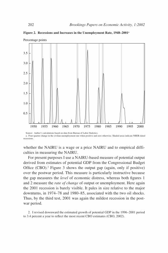
Figure 2 shows an analogous measure for the unemployment rate. Herethe line shows increases in the four-quarter unemployment rate whenunemployment is rising and is at zero when it is falling; recessions areagain shown as shaded areas. This measure produces several false posi-tives, indicating that the unemployment rate is a less reliable indicator of

200 Brookings Papers on Economic Activity, 1:2002

1. NBER Business Cycle Dating Committee, March 11, 2002, at www.nber.org/cycles/recessions.html.

0675-04 BPEA/Nordhaus 7/22/02 1:13 PM 00

NBER recessions than real GDP growth. A slight modification wouldhold that when the four-quarter change in the unemployment rate isgreater than 1 percentage point, we have a reliable indicator of recession.By the unemployment rate standard, the last two recessions have been themildest in postwar history.

A final indicator of business cycles is the output gap, which measuresthe percentage difference between potential and actual GDP. The analy-sis of gaps is controversial because of the difficulties in defining andmeasuring potential output. Some classical approaches hold that output isessentially always equal to its potential, so that output gaps either are def-initionally zero or quickly disappear. Among schools that believe in gaps,some have measured the gap by interpolating between output peaks. Oth-ers use Okun’s law and calculate the difference between actual outputand the output that would be consistent with a benchmark unemploymentrate such as the NAIRU; this in turn gives rise to other ambiguities about

William D. Nordhaus 201

Figure 1. Recessions and Declines in Real GDP Growth, 1948–2001a

Source: Author’s calculations based on data from Bureau of Economic Analysis, National Income and Product Accounts(NIPA).

a. Two-quarter growth rate of real GDP when negative and zero otherwise. Shaded areas indicate NBER-dated recessions.

-7

-6

-5

-4

-3

-2

-1

1950 1955 1960 1965 1970 1975 1980 1985 1990 1995 2000

Percent a year

0675-04 BPEA/Nordhaus 7/22/02 1:13 PM Page 201

whether the NAIRU is a wage or a price NAIRU and to empirical diffi-culties in measuring the NAIRU.

For present purposes I use a NAIRU-based measure of potential outputderived from estimates of potential GDP from the Congressional BudgetOffice (CBO).2 Figure 3 shows the output gap (again, only if positive)over the postwar period. This measure is particularly instructive becausethe gap measures the level of economic distress, whereas both figures 1and 2 measure the rate of change of output or unemployment. Here againthe 2001 recession is barely visible. It pales in size relative to the majordownturns, in 1974–78 and 1980–85, associated with the two oil shocks.Thus, by the third test, 2001 was again the mildest recession in the post-war period.


2. I revised downward the estimated growth of potential GDP in the 1996–2001 periodto 3.4 percent a year to reflect the most recent CBO estimates (CBO, 2002).

Figure 2. Recessions and Increases in the Unemployment Rate, 1948–2001a

Source: Author’s calculations based on data from Bureau of Labor Statistics.a. Four-quarter change in the civilian unemployment rate when positive and zero otherwise. Shaded areas indicate NBER-dated

recessions.

0.5

1.0

1.5

2.0

2.5

3.0

3.5

1950 1955 1960 1965 1970 1975 1980 1985 1990 1995 2000

Percentage points


2001: The Highest Trough

A second unusual feature of the 2001 recession was that the level ofoutput was relatively high as the economy emerged from recession. Inother words, at the trough of the recession, which I assume was the fourthquarter of 2001, the gap between actual output and potential output wasrelatively small.

Figure 4 shows the estimated GDP gap at the trough of each postwarNBER recession, again assuming that the trough of the latest recessioncame in the fourth quarter of 2001. The results are striking. The trough ofthe 2001 recession was as close to potential output as in any postwarrecession; only the 1954 recession showed as small a gap. Indeed, to afirst approximation, the economy was at its potential at the trough of the2001 recession. This striking fact indicates, first, that the recession was


Figure 3. Recessions and Real Output Gaps, 1948–2001a

Source: Author’s calculations based on data from Bureau of Economic Analysis, NIPA, and CBO (2001, 2002).a. Percentage difference between potential GDP and actual GDP when positive and zero otherwise. Potential real GDP estimates

through 1996 are from CBO (2001) and thereafter grow at a 3.4 percent annual rate, as assumed in CBO (2002).

1

2

3

4

5

6

7

1950 1955 1960 1965 1970 1975 1980 1985 1990 1995 2000

Percent of potential GDP


indeed very mild, with only a small decline in output (as figure 1 showed)and, second, that it started from a peak at which output was extremelyhigh and unemployment very low for a peacetime period. This point canbe expressed in a different way, by noting that the unemployment rate inthe fourth quarter of 2001 was 5.6 percent, close to most estimates of thecurrent NAIRU, which cluster around 51⁄2 percent.

By contrast, the Federal Reserve Board’s index of industrial capacityutilization does not corroborate this high level of factor utilization, butrather was close to the average for a recession trough at the end of 2001.However, industrial production makes up only a small slice of the econ-omy—approximately 20 percent of GDP—and this slice consists largelyof tradable goods for which domestic capacity utilization is increasinglyirrelevant (oil production being the most obvious example). The mostimportant limit on capacity is likely to be labor rather than manufacturingcapital. Thus the low rate of capacity utilization is little comfort for thosewho worry about the inflationary risks that would be encountered if therewere a brisk, defense spending–led recovery over the next few years.


Figure 4. Output Gap at Trough of Recession for Ten Postwar Recessionsa

Source: Author’s calculations based on data from the Bureau of Economic Analysis, NIPA, and CBO (2001, 2002).a. Calculated as the percentage difference between potential real GDP and actual real GDP. The potential GDP series is

described in figure 3.

0

1

2

3

4

5

6

7

1949:4 1954:2 1958:2 1961:1 1970:4 1975:1 1980:3 1982:4 1991:1 2001:4

Percent of potential GDP


Is It Time to Rethink the Definition of Recessions?

By NBER business-cycle standards, the 2001 downturn, however mild,falls in the same category as the much deeper contractions of 1933 or1982. This observation might well lead one to conclude that the tradi-tional NBER business-cycle methodology, which identifies only peaksand troughs without reference to the depth or severity of the downturn, isoutdated. This approach was reasonable given the meager and incompletedata available when Wesley Clair Mitchell and Arthur Burns invented thebusiness cycle dating approach several decades ago.3 However, in light ofthe plentiful, timely, and comprehensive data available today, surely wecan do better than simply flying a green flag or a red flag depending uponthe slope of the underlying economic indicators. In this I am reminded ofTjalling Koopmans’s critique of Burns and Mitchell more than a half-century ago: “[E]ven for the purpose of systematic and large scale obser-vation of such a many-sided phenomenon [as business cycles], theoreticalpreconceptions about its nature cannot be dispensed with, and the authorsdo so only to the detriment of the analysis.”4

An alternative approach would be to develop quantitative criteria thatwould allow one to categorize business downturns in a manner analogousto the Saffir-Simpson hurricane scale. This suggestion in part reflects thefinding that the volatility of output, along with the frequency and severityof business cycles, is declining in the United States.5 It also is based onthe view that business cycles are more like hurricanes than like pregnan-cies:6 far from being a simple two-state phenomenon, they are extremelydiverse in their shape, size, and duration. The proposal is in part moti-vated by the view that business-cycle dynamics are often grounded inlocal instabilities that can grow into full-scale disturbances if they areunchecked or trigger yet further instabilities.

As a start, I would propose categorizing recessions according to a scaleof I (a pause in economic activity) to V (severe depression). Based on the


3. See in particular Mitchell (1913), which marks the beginning of the business cycledating tradition. The most systematic study was that of Mitchell and Burns (1946).

4. Koopmans (1947, p. 163).5. See Blanchard and Simon (2001).6. The pregnancy, or two-state, view is associated with Hamilton (1990). A look at fig-

ures 1 through 3, or a more systematic examination of the transition matrix between differ-ent states of the economy, would quickly reject the view that all recessions are a singlestate.


size and duration of the declines in growth rates and gaps in output,employment, and unemployment, I would tentatively classify the histori-cal recessions in the United States as follows:

Category I (pause in economic activity) 1963, 1967, 2001?Category II (mild downturn) 1961, 1970Category III (typical recession) 1949, 1954, 1958, 1975, 1991Category IV (deep and prolonged recession) 1980–82Category V (depression) 1930s

This “new view” of business cycles as heterogeneous in duration andseverity would also allow us to view periods of recovery as highly differ-entiated. In the present recovery, which probably started in late 2001,there is little room for the economy to expand before it hits the inflation-ary danger zone. As a result, monetary policymakers are likely to hit thebrakes sooner and harder than they did in earlier recoveries. And the stim-ulus package passed in March 2002 will be the latest exhibit for the argu-ment that fiscal policy measures are generally implemented too much, toolate, and with the wrong sign.

Deciphering the Profits Numbers

Part of the exhilaration of the 1990s was due to the rapid growth in cor-porate earnings. For the period 1992–2000, profits as reported in theNational Income and Product Accounts (NIPA) grew at an average rate of8 percent a year. Over the same period, earnings per share as reported byStandard & Poor’s grew at 15 percent a year.

Before digging into the concepts and numbers, it must be recognizedthat “profits” is a most elusive concept. There are at least four importantdefinitions: profits for accounting purposes, profits for tax purposes, prof-its as measured in the NIPA, and economic profits. The first three arewidely discussed, whereas the fourth is usually ignored. From the point ofview of the corporation (rather than its shareholders), a reasonable defini-tion of economic profits would be distributions to shareholders plus thechange in real net worth from one period to the next. Such a definition dif-fers from the other three measures of profits in important ways. Unlikeeconomic profits, NIPA profits exclude real asset appreciation; account-ing profits embody many concepts inappropriate to an economic defini-tion, of which the treatment of depreciation and capital appreciation are




7. Petrick (2001, pp. 16–20) provides a full discussion.8. When firms enter or leave the S&P 500, continuity of the share price index is

achieved by creating a total market “divisor” to link different periods together. If the price-earnings ratios of entering and leaving firms are unequal, this will induce a change in theprice-earnings ratio of the aggregate. The procedure is discussed at www.spglobal.com/5sec3.pdf. An examination of the divisor suggests that firm substitutions are substantial.The divisor rises when new firms enter with higher value than the exiting firms, when com-panies issue new shares, or when two S&P companies merge. The size of the divisor hasgrown by about 4 percent a year in the last decade, but there is no empirical evidence on thereasons for this growth.

two; and both tax and accounting profits treat capital gains inappropri-ately by excluding some accrued gains and including gains that are dueonly to price level changes.

In practice, the only available comprehensive measures of profits areNIPA profits and S&P profits. Several versions of NIPA profits are avail-able: NIPA profits after taxes exclude adjustments for inventory valuationand capital consumption, whereas NIPA adjusted profits after taxesinclude these adjustments. There are two published versions of S&P prof-its. The first is operating earnings, which are more or less the earningsfrom continuing operations and exclude the impact of cumulativeaccounting changes, discontinued operations, extraordinary items, andspecial items; the second is earnings “as reported,” which include theseitems. The earnings used in price-earnings ratios are the reported variant.

Although S&P and NIPA profits are often compared, they differ sub-stantially in their definitions, methodologies, source data, and coverage.7 Iwill highlight some of the major differences. First, the S&P data coveronly 500 large corporations, whereas the NIPA data cover the entire econ-omy, even including very small subchapter S corporations. Second, NIPAprofits are designed to measure the income from current productionearned by domestic corporations, whereas S&P earnings are measured ona financial accounting basis. Third, NIPA profits exclude capital gains,which can be substantial; in 1998, for example, corporations reported$205 billion of capital gains as part of their profits. Fourth, the S&P datacome from a changing panel of firms, which requires a complicated chain-ing procedure that ensures comparability of market value over time butdoes not ensure comparability of earnings.8

The fifth difference is seen in the capital consumption adjustment andthe inventory valuation adjustment, which together measure the differ-ence between economic cost and accounting cost. Although these series



are generally quite smooth, the capital consumption adjustment jumpedfrom $13 billion to $186 billion in the fourth quarter of 2001; thisincrease led to a huge difference between adjusted NIPA profits and S&Pearnings. A sixth difference is source data: the NIPA data are in principlederived from tax returns whereas the S&P data are derived from financialaccounts. On the other hand, early estimates of NIPA profits are based onfinancial accounts data, and they are often revised, whereas Standard &Poor’s apparently never revises its data or takes into account restatementsof earnings.

Figure 5 shows these four measures of after-tax corporate profits over1985–2001. The top two lines are NIPA profits after taxes, adjusted (theupper line) and unadjusted for capital consumption and inventory valua-tion (the second line from the top). The bottom two lines are operating(the second from the bottom) and reported after-tax earnings (the bottomline) of the companies in the S&P 500. The data for the fourth quarter of2001 show divergent trends in these profits numbers. After-tax adjustedNIPA profits increased 6 percent on a year-over-year basis, whereas thethree other series declined by between 23 and 36 percent. The NIPA fig-ures were affected by a one-time tax change arising from the March 2002stimulus package, which allowed firms to expense 30 percent of coveredinvestments. Because the source data for the NIPA are extremely sparsefor the most recent period, it seems likely that the latest NIPA profits datawill be significantly revised in the next few years.

All of the different profits series have taken a major dive in the last fewyears. As a share of GDP, the two NIPA series peaked in 1997 at just over7 percent; since then their share has declined by about one-third, or byslightly more than 2 percentage points through the third quarter of 2001.The S&P earnings share peaked three years later. The lag of S&P earningsbehind NIPA profits was not a feature of earlier cycles and has no obviouseconomic rationale.

What might have caused this most unusual pattern of earnings? Theobvious suspicion is that the rapid rate of “innovation” in accountingtechniques has distorted the timing of reported earnings over the last fewyears. Every day, the newspapers recount a host of new techniques bywhich companies have bolstered reported earnings. Some of the mostegregious examples of these “Not Generally Accepted Accounting Prin-ciples,” or NGAAP, include swapping capital assets such as natural gasfutures contracts (Enron) or “dark” fiber optic networks (Global Cross-


ing, Qwest, Enron) and capitalizing the outflow while recognizing theinflow as current revenue; increasing the salvage value of trucks overtime (Waste Management); recognizing the returns to pension plans asoperating income (IBM); recording sales of products still in research(McKesson HBOC); changing the pattern of accounting revenue fromrentals (Xerox); increasing the value of the unused capacity of landfillseven as they fill up (Waste Management); reporting happy pro formanumbers when the reality is unpleasant (Amazon.com, Yahoo, and Qual-comm among a crowd of other dot-coms dead and alive); using funds setaside as merger and acquisition reserves to increase operating income(Cendant); and doubling earnings by simply neglecting to includeexpenses (BroadVision).9


9. The Securities and Exchange Commission’s report on its analysis of Waste Manage-ment’s NGAAP was highlighted in the New York Times (Kurt Eichenwald, “Waste Man-agement Executives Are Named in S.E.C. Accusation,” March 27, 2002, p. C1). Swaps of“dark” fiber optic capacity were also described in the New York Times (David Barboza andBarnaby J. Feder, “Enron’s Swap with Qwest Is Questioned,” March 29, 2002, p. C1).

Figure 5. Alternative Concepts of After-Tax Corporate Profits, 1985–2001

Source: Bureau of Economic Analysis, NIPA, and Standard & Poor’s.a. Includes inventory valuation adjustment and capital consumption adjustment.

100

200

300

400

500

600

1987 1989 1991 1993 1995 1997 1999 2001

Billions of dollars a year

NIPA adjusted a

NIPA unadjusted

S&P operating

S&P reported


Aside from enrichment of the few and depleted pension plans of themany, did NGAAP affect the aggregate numbers? Figure 5 suggests thatNGAAP earnings have indeed infected total reported S&P earnings. Itseems clear that the peak in S&P earnings lagged behind the peak inNIPA earnings because companies were “managing” their earnings (inthis context, preventing an accounting decline in earnings). However,they could only prevent the earnings decline for a couple of years, afterwhich they ran out of gimmicks, or the accountants—or else analysts andthe Securities and Exchange Commission—began to blow their faintwhistles.

Another interesting feature of the recent profits data, also shown in fig-ure 5, is that reported profits are currently extremely low relative to oper-ating profits. The difference between reported and operating profits isprimarily one-time charges that companies take to correct for past busi-ness or accounting errors—as they hang out their dirty laundry, so tospeak. The declining ratio of reported to operating profits late last yearprobably reflects the tendency of companies to purge their earnings andbalance sheets of questionable elements in light of the Enron scandal. Thesize of the write-downs became truly enormous in late 2001 and early2002. Announced or estimated write-downs so far include $54 billion forAOL Time Warner, $20 billion to $30 billion for Qwest, $15 billion to$20 billion for WorldCom, $10 billion for VeriSign, $5 billion for AT&T,$3 billion for Cisco, and the list goes on. Analysts are bruiting about atotal price tag of $1 trillion for the Great Balance Sheet Purge of 2002.10

In considering future earnings prospects, one must take into accountboth the cyclical depression of profits and the likelihood that reportedprofits are contaminated by an accounting purge. Figure 6 shows the his-torical trend in the ratio of quarterly S&P (reported) earnings per share toGDP and unadjusted NIPA earnings to GDP, where both are scaled sothat the average ratio over the 1949–2001 period equals 100. Again,NBER recessions are shown as shaded areas.

The two series in figure 6 move together during most of the period until1990. Since 1990 the pattern looks quite different, with the NIPA num-bers largely skirting the 1991 recession. The most dramatic difference


10. “Buying Binge Could Cost Corporate America $1 Trillion,” USA Today, April 5,2002, p. 1B.


comes at the end of the period, with the huge drop in reported S&P earn-ings, presumably due primarily to the balance sheet purge.

To obtain a more realistic estimate of earnings than the reported S&Pearnings, I have calculated a series of S&P earnings corrected for thebusiness cycle and accounting purges. This series, which I call “correctedS&P earnings,” was calculated from a regression of the logarithm of S&Preported earnings on the logarithm of unadjusted NIPA profits after taxes,time, a cyclical variable, and a constant. I then forecast corrected S&Pearnings by assuming that unadjusted NIPA profits are set at their cycli-cally adjusted level and that S&P profits are at the level forecast on thebasis of cyclically corrected NIPA profits. In effect, this uses NIPA prof-its as a proxy for cleaned-up S&P reported earnings. I then forecast S&Pprofits for the period 2001:4 through 2002:4. The projection assumes thatreal GDP grows one-half percentage point faster than potential output


Figure 6. Trends in NIPA and S&P 500 After-Tax Profits Relative to GDP,1949–2001a

Source: Author’s calculations based on data from Bureau of Economic Analysis, NIPA, and Standard & Poor’s.a. Shaded areas indicate NBER-dated recessions.b. Each series is divided by GDP and scaled so that the average of the new series is 100 over 1949–2001.

20

40

60

80

100

120

140

160

180

1950 1955 1960 1965 1970 1975 1980 1985 1990 1995 2000

Indexb

NIPA unadjusted

S&P reported


during 2002. This procedure, along with recent and projected values ofS&P profits, is described in more detail in appendix A.

This experiment indicates that reported S&P earnings were indeeddepressed at the end of 2001 for a combination of cyclical and accountingreasons. Reported S&P earnings for 2001 were about 30 percent belowthe estimate of corrected, or “clean,” S&P earnings. If earnings were torebound to their forecast corrected levels at the end of 2002, they wouldbe 55 percent higher than their levels in 2001:4.

In summary, there has been a substantial fall in profits since their peakin the late 1990s. The recent pattern of profits suggests that financialfinagling has infected the reported profits figure, and in particular theaggregate financial accounting numbers, in the last decade. Perhaps thebest summary would be to recall the wisdom in John Kenneth Galbraith’ssaying that depressions catch what the auditors missed.

Party Time Continues in Equity Markets

Robert Shiller has argued, in his influential and exquisitely timed book,Irrational Exuberance, that equity prices in the 1990s got seriously out ofline with economic fundamentals.11 In Shiller’s most recent analysis withJohn Campbell, the bears of academe write:

We believe that our original testimony and article are even more relevant today[March 2001]. Valuation ratios moved up in the year 2000 to levels that wereabsolutely unprecedented, and are still nearly as high as of this writing at thebeginning of 2001. Even allowing for the possibility that the economy andfinancial markets have undergone some structural changes, these ratios imply astronger case for a poor stock market outlook than has ever been seen before.12

What has changed since then? The major developments since early2001 have been the steep decline in earnings discussed in the last sectionalong with a sideways movement of stock prices. To illuminate theCampbell-Shiller thesis, I have looked at the real return on equities andthe yield spread between equities and safe assets. The basic assumptionin this analysis is that the earnings-price ratio is a reasonable estimate of


11. Shiller (2001).12. Campbell and Shiller (2000, p. 1).


the forward-looking real return on equities,13 where this is defined as theexpected total return per share (dividends plus capital gains) corrected formovements in the general price level.

The derivation of this result is presented in appendix B, but the reason-ing can be described verbally. Begin with the market value of the firm, theassets of the firm, and the earnings or profits on assets. For this purpose,assets should include all tangible and intangible assets. Let q be the ratioof the market value of the firm to its total assets, where marginal q appliesto new investments and average q applies to old assets. It will simplify thediscussion to assume that firms have no debt and to ignore taxes.

The conditions under which the prospective return on equity equals theearnings-price ratio are neither obvious nor obviously correct. To beginwith, the theory needs to assume that earnings are an accurate measure oftrue profits, which definitely gets the exercise off to a bad start. One sim-ple case where the earnings-price ratio is a good forward-looking estimateof the return on equities is that where marginal q equals 1, the q ratios areconstant, and the expected rate of return on capital is constant. Some othercases are discussed in appendix B. In reality, the q ratios and the expectedreturn on capital are likely to bounce around a great deal, and so the actualreturns on equity will differ from the earnings-price ratio. In terms ofmarket conditions in early 2002, the major reasons to believe that equityreturns will differ from the earnings-price ratio are, first, if the rate ofprofit rises because it is currently depressed, and second, if average q fallsbecause assets are currently overvalued.

With these theoretical considerations behind us, figure 7 shows twovariants of the estimated real forward-looking return on equities over thepostwar period. Variant 1 is the earnings-price ratio for the S&P 500 usingquarterly earnings.14 Variant 2 takes variant 1 and performs the correctionfor the business cycle and for accounting problems discussed in the lastsection.


13. Other popular approaches sometimes compare the earnings-price ratio or thedividend-price ratio with nominal interest rates. These approaches make the fundamentalerror of confusing real and nominal magnitudes—in effect assuming that the prices ofgoods and dollar returns are constant.

14. The published measure of earnings in the S&P numbers (such as that used in calcu-lating price-earnings ratios) uses a four-quarter trailing average of earnings. In the presentanalysis I take seasonally adjusted current quarterly earnings at an annual rate and dividethis by the current-period stock price index.


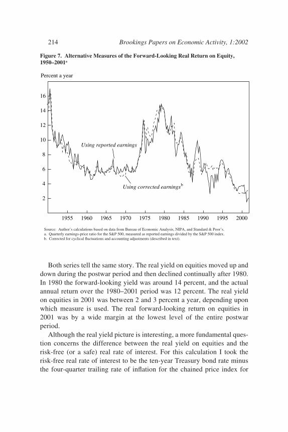
Both series tell the same story. The real yield on equities moved up anddown during the postwar period and then declined continually after 1980.In 1980 the forward-looking yield was around 14 percent, and the actualannual return over the 1980–2001 period was 12 percent. The real yieldon equities in 2001 was between 2 and 3 percent a year, depending uponwhich measure is used. The real forward-looking return on equities in2001 was by a wide margin at the lowest level of the entire postwarperiod.

Although the real yield picture is interesting, a more fundamental ques-tion concerns the difference between the real yield on equities and therisk-free (or a safe) real rate of interest. For this calculation I took therisk-free real rate of interest to be the ten-year Treasury bond rate minusthe four-quarter trailing rate of inflation for the chained price index for


Figure 7. Alternative Measures of the Forward-Looking Real Return on Equity,1950–2001a

Source: Author’s calculations based on data from Bureau of Economic Analysis, NIPA, and Standard & Poor’s.a. Quarterly earnings-price ratio for the S&P 500, measured as reported earnings divided by the S&P 500 index.b. Corrected for cyclical fluctuations and accounting adjustments (described in text).

2

4

6

8

10

12

14

16

1955 1960 1965 1970 1975 1980 1985 1990 1995 2000

Percent a year

Using reported earnings

Using corrected earningsb


GDP.15 I call the difference between the real equity rate and the real bondrate the “equity spread,” but others might call it the equity premium. Stan-dard doctrine holds that the equity spread should be positively associatedwith the systematic risk of equities and should definitely be positive.

Figure 8 shows two different calculations of the equity spread over thelast half century using the two series on the forward-looking return toequities from figure 7. The story told here is slightly different from that infigure 7. The equity spread declined sharply in the early 1980s with thehigh real interest rates of that period. The spread then ranged between2 and 4 percentage points in the late 1980s, and it has gradually declinedsince then. At the end of 2001, the equity spread was close to zero—eitherslightly negative if the uncorrected earnings figure is used or slightly pos-itive if the corrected figure is used.

According to the most recent data, and focusing on the corrected seriesin figure 8, the spread has moved up slightly since the peak of the equitiesmarket in the spring of 2000. In the first quarter of 2000, the spreadbetween equities and bonds was a negative 157 basis points, whereas bythe end of 2001 the spread had moved to a positive 47 basis points. Forthe latest period (mid-April 2002, not shown), bond yields have risen andthe corrected equity spread has dipped back down to minus 30 basispoints.16


15. Alternative approaches to measuring inflation would use the price index for corpo-rate product or the consumer price index rather than the chained price index for GDP, andalternative interest rates would be the real short-term interest rate or Treasury real interestbonds. These would change the levels of the curves but would not change the general trend.For example, over the last five decades, the real one-year Treasury rate has averaged about70 basis points less than the ten-year rate, and so the spread would be that much higher overthe period. The average rate of inflation for the GDP price index was 0.3 percentage pointlower than that for the consumer price index for the last five decades. This suggests that theestimated returns or spreads might differ by as much as 100 basis points a year if differentindexes were employed.

16. Changes in the spread could arise from many factors. Changes in risk aversion,changing expectations of real growth in the returns on equities, and changing perceivedriskiness of stocks are the fundamental economic factors (as distinguished from technicalor psychological factors). Is seems hard to derive sound reasons why any of the three fun-damental factors have changed so dramatically in favor of equities in recent years. It hasbeen argued that the equity premium was excessive during most of the twentieth century,but no theory would predict a zero equity premium. Nor does it seem plausible that a modelwith a constant equity premium fits recent experience.


It is useful to compare these estimates with surveys of what economicsand finance professors actually believe about the stock market’sprospects. According to Ivo Welch’s survey of 510 economics andfinance professors conducted in August 2001, the average equity spreadwas estimated to be 3.4 percentage points for a one-year horizon and4.7 percentage points on a thirty-year horizon.17 About 6 percent believedthat the equity premium would be negative at a one-year horizon, andnone believed that it would be negative at a thirty-year horizon. Clearly,neither Campbell and Shiller’s writings, nor Shiller’s book, nor actualearnings-price ratios have made much of a dent in the optimism of financeprofessors.


17. Welch (2001). The survey question was “I expect the average equity premium (i.e.,expected return on the market net of the short-term interest rates) over the next 1 year to be. . . .” The market was taken to be the S&P 500.

Figure 8. Forward-Looking Spread between Equities and Bonds, 1952–2001a

Source: Author’s calculations based on data from Bureau of Economic Analysis, NIPA; Board of Governors of the FederalReserve; and Standard & Poor’s.

a. Forward-looking return on equities (from figure 7) minus the real interest rate on ten-year Treasury bonds.b. Corrected for cyclical fluctuations and accounting adjustments (described in text).

-2

0

2

4

6

8

10

12

14

1955 1960 1965 1970 1975 1980 1985 1990 1995 2000

Percentage points a year

Using reported earnings

Using corrected earningsb



The overall results suggest that the prospective yield on equities isabout equal to that on safe assets. At the same time, the prospective realyield on equities is at its low point of the last half-century. The overvalu-ation of equities has improved slightly since Campbell and Shiller’s lastgloomy prognostication, but it hardly looks rosy.

Summary

The basic features of the current recovery are clear. The downturn of2001 was extremely mild, somewhere between a category I and a cate-gory II recession on the economic hurricane scale. Because the economybegan the recession at an unusually high peak, and because the downturnwas short and mild, the economy at the trough of the recession (assumedto have occurred in late 2001) was close to full employment in terms ofinflationary pressures.

Corporate profits are depressed relative to their peaks in the 1990s, andthe forward-looking real return on equities is about equal to the risk-freereal rate of interest, that is, the rate on medium-term U.S. governmentbonds. For those who make their living in financial markets, this is notgood news. Bonds are likely to get hit quickly if the economy recoverssharply and the Federal Reserve follows its script of preempting inflation-ary output growth. Stocks are still overvalued relative to most of the post-war period—and this at a time of significant prospects of financialtightening and growing concern about what bad news still hides inside theblack box of earnings statements. It seems unlikely that the United Stateswill soon return to the bubbly days of the late 1990s.

A P P E N D I X A

Derivation of Corrected S&P Earnings

S&P REPORTED PROFITS ARE affected both by the business cycle and byaccounting fraud and low misdemeanors. To estimate a series of “clean,”or corrected, S&P profits, I use NIPA profits as a proxy variable. In whatfollows, Pt is measured S&P profits, Pt* is true S&P profits, and Pt*CC iscyclically corrected true S&P profits. NPt and NPt

CC are NIPA unadjusted


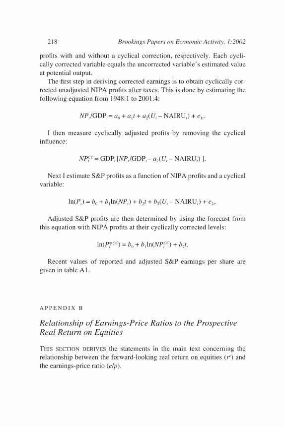
profits with and without a cyclical correction, respectively. Each cycli-cally corrected variable equals the uncorrected variable’s estimated valueat potential output.

The first step in deriving corrected earnings is to obtain cyclically cor-rected unadjusted NIPA profits after taxes. This is done by estimating thefollowing equation from 1948:1 to 2001:4:

NPt /GDPt = a0 + a1t + a2(Ut – NAIRUt) + e1t.

I then measure cyclically adjusted profits by removing the cyclicalinfluence:

NPtCC = GDPt [NPt /GDPt – a2(Ut – NAIRUt) ].

Next I estimate S&P profits as a function of NIPA profits and a cyclicalvariable:

ln(Pt) = b0 + b1ln(NPt) + b2t + b3(Ut – NAIRUt) + e2t.

Adjusted S&P profits are then determined by using the forecast fromthis equation with NIPA profits at their cyclically corrected levels:

ln(Pt*CC) = b0 + b1ln(NPtCC) + b2t.

Recent values of reported and adjusted S&P earnings per share aregiven in table A1.

A P P E N D I X B

Relationship of Earnings-Price Ratios to the ProspectiveReal Return on Equities

THIS SECTION DERIVES the statements in the main text concerning therelationship between the forward-looking real return on equities (re) andthe earnings-price ratio (e/p).



Let qA be average q, qM marginal q, p the price per share, k total assetsper share, rk earnings per unit of asset per year, re the total return on equi-ties per year, and d the dividend payout ratio. Assume that there are nobonds and no taxes. We consider the real value of the variables in periodst and t + 1.

To begin with, the earnings-price ratio in the first period is equal to theratio of the return on assets to average q:

To derive the total return on equities, note that the price per share in thefirst period is pt = kt qA

t . Reinvested earnings are (1 – dt )rkt kt , so that the

price per share in the second period is

The total return on equities between the first and the second period isthen

( ) ( – ) .2 11 1 1p k q d r k qt t tA

t tk

t tM

+ + += +

( ) / / / .1 e p r k q k r qt t tk

t tA

t tk

tA= =


Table A1. As-Reported and Corrected S&P Earnings per Share, 1999–2002Dollars

Quarter As reported Correcteda Ratio (percent)

1999:1 10.72 9.02 1191999:2 12.23 9.06 1351999:3 12.39 9.10 1361999:4 12.86 9.65 1332000:1 13.43 9.78 1372000:2 13.18 9.97 1322000:3 14.24 10.00 1422000:4 9.13 9.73 942001:1 8.97 9.23 972001:2 4.72 9.20 512001:3 5.43 8.83 622001:4 5.70 8.40 682002:1 n.a. 8.50 n.a.2002:2 n.a. 8.61 n.a.2002:3 n.a. 8.71 n.a.2002:4 n.a. 8.82 n.a.

Source: Author’s calculations based on data from Bureau of Economic Analysis, NIPA, and Standard & Poor’s.a. Corrected for cyclical fluctuations and accounting adjustments (as described in text). Values for 2002 are forecast.

0675-04 BPEA/Nordhaus 7/22/02 1:13 PM 9

One polar case is where marginal q is 1 even though average q isgreater than 1. This case would apply when the firm has supernormalprofits in one area (say, on a patent or a piece of software) but is unable toleverage that market power into other markets. In this case, as long asaverage q is constant, re = rk/qA = e/p. That is, the return on equities isthe rate of return on existing assets divided by average q, which is theearnings-price ratio. This case is interesting because the return on equi-ties diverges from the return on capital.

An alternative view would come about when marginal q is differentfrom 1. This case might apply for a firm that has been able to extend itsmonopoly into other markets. In this case, re = e/p when d = 1, or whereall earnings are paid out as dividends.

We can use numerical values to determine the forward-looking returnfor other cases. For large corporations, assume that the rate of return onassets is 8 percent a year after tax, average q is 1.6, and the dividend pay-out ratio is 0.5. Suppose that marginal q is 1.3, which would imply thatfirms could project some but not all of their market power into newinvestments. Applying equation 3 then yields a forward-looking return of5.8 percent a year, which exceeds the earnings-price ratio of 5 percent.

As a final case, assume that q deviates from unity because of specula-tive bubbles or anti-bubbles, and that average q regresses back toward 1with a decay rate of 10 percent a year; that is, on average q moves 10 per-cent of the way from (q – 1) to 1 each year. Then, using the same numbersas in the last paragraph, the forward-looking real return on equities wouldbe 2 percent a year rather than 5.8 percent a year and would be below theearnings-price ratio.

The main point is that the forward-looking return on equities generallyinvolves both average and marginal q. And where average q is very high,the forward-looking return can be well below the rate of return on capital r.

( )[ ( – ) ] / –

( / ) [ ( – ) ] / – .3

1 1

1 11 1 1

1 1

r d r k k q d r k q k q

q q d r d r q qte

t tk

t t tA

t tk

t tM

t tA

tA

tA

t tk

t tk

tM

tA

+ + +

+ +

= + += + +


0675-04 BPEA/Nordhaus 7/22/02 1:13 PM 0

Comment and Discussion

George L. Perry: William Nordhaus’s paper covers several relatedaspects of the current economic scene: the recent recession and currentrecovery, the behavior of profits during and leading up to the recession,and the prospects for the stock market in the recovery. He offers provoca-tive ideas on all fronts.

Nordhaus compares the ten postwar recessions identified and dated bythe NBER by examining four broad measures of economic loss: declinesin real GDP, declines in employment, increases in unemployment, andpositive output gaps as measured by the CBO. Output and employmentdeclines track NBER-dated recessions very closely. Increases in unem-ployment lag these other measures of change, especially when measuredover four quarters as in Nordhaus’s figure 2, and this indicator yields sev-eral false-positive identifications of NBER recessions. The pattern of out-put gaps bears little relation to that of NBER recessions because thesegaps usually remain positive for extended periods after a recessiontrough. However, if properly measured, the output gap would provide asummary indicator of overall economic loss.

From this broad-brush comparison of recessions, Nordhaus draws botha particular and a general message. The particular message is that lastyear’s recession was the mildest of the postwar period and that at itstrough, which he takes to be the fourth quarter of 2001, the economy wasvirtually at its potential output. I will say more about that later. The gen-eral message is that the NBER’s approach to recession dating is outdated:recessions differ so much in their severity and length that a richer classifi-cation scheme is called for; meanwhile advances in economic science and

221


data availability allow us to do a better job of classifying recessions thanthe pioneers of business cycle measurement were able to do. Nordhaussuggests developing quantitative criteria that would allow business cycledownturns to be classified more like hurricanes are, with several grada-tions reflecting their severity.

Nordhaus gives the impression that a lot is at stake in refining our def-inition of recessions and applying more data to the task of identifying andclassifying them. He hints that business-cycle dynamics could reflect thepropagation of small impulses into large outcomes, so that identifyingincipient virulent recessions would have important benefits. As a scien-tific matter, that is an important question and related to the more generalquestion of whether periods of recession are special, in the sense thatagents respond differently in recessions than at other times. That wouldbe a reason to care a lot whether we were in or heading for such a period.If we could predict emerging weakness better, we should. But that goal isand always has been hotly pursued. It has nothing to do with classifyingdownturns according to severity after the fact.

Turning to that more modest task, I agree with Nordhaus that theNBER should look not only at changes in but also at levels of economicactivity in identifying recessions. And that criticism holds true even if wedo not expand the NBER dating committee’s limited mandate, which is toidentify “a significant decline in activity spread across the economy”(emphasis added). I have always believed that one strength of recessiondating by a committee of experts was that they were free to consider anyand all evidence of recession. There were surely stretches in the first halfof the 1930s when employment rose, but we all speak of that whole periodas the Great Depression. And if we took away several months of dead-catbounce in the economy that followed its precipitous decline in the firsthalf of 1980, the whole of 1980–82 would be one recession, not two asjudged by the NBER. It felt like one recession at the time. I see no reasonother than precedent for the experts to look only at whether measures suchas sales and employment are falling in identifying when a recession startsand, more important, when it ends.

However, going from principles to practice, I find the CBO output gapthat Nordhaus uses in analyzing the level of economic utilization to beinadequate. The main problem is that empirical estimates of the NAIRUare the anchor for estimating potential output and the output gap, andthose estimates are not reliable. The best thing Alan Greenspan has done



as Federal Reserve chairman was to distrust the conventional wisdom in1995 about what unemployment rate was too low. I would have thoughtthat experience, along with some really good papers on the subject, wouldhave persuaded Nordhaus to distrust the NAIRU estimates, too. An addi-tional problem in judging the room for expansion today is the uncertaintyabout how fast the productivity trend is rising.

What other issues does Nordhaus raise or imply? The recent recessionwas marked by unusually good productivity gains, and therefore employ-ment was weak relative to output. How to weight the two in identifyingrecessions is open to disagreement, but it is not a matter of applying morescience. My sense of what we are after would look at both employmentand unemployment. Nordhaus’s more nuanced approach might favor out-put, since it does not end with a simple yes or no on recession.

Another issue that Nordhaus raises about NBER dating is its timeli-ness, but I find this overdone. The Federal Reserve does not wait for theNBER when it decides whether to act. So the dating committee need notoverly concern itself about when we knew we were in trouble in real time,but rather about when, as a matter of history, to identify the turningpoints. After all, that is what NBER dating is mainly about, and it pro-vides a useful way to organize ideas and present results. The deliberatespeed with which the committee makes its judgments is appropriate forthat purpose. Some people think that identifying a recession or a recoveryhas political consequences, but I doubt it. President George Bush, Sr., wasin trouble in 1992 not because the NBER had not announced that therecession was over, but because unemployment was still rising as he cam-paigned, and he was seen as not caring much about it.

Nordhaus’s particular message about last year’s recession is consistentwith how he views current economic prospects. Because the recoverystarts with unemployment very near his estimated NAIRU, he sees littleroom for the economy to expand. He concedes that capacity utilizationrates tell a different story, but he reasons that labor rather than capital willbe the limiting factor and that any rapid expansion led by defense spend-ing will soon run into rising interest rates from the Federal Reserve. As Isee it, however, employment has fallen a lot, at the trough the economywas far from its potential, and ample spare capacity is just what risingdefense spending needs. The Federal Reserve might raise rates beforelong. But since that is what it usually does, it might not surprise marketsor have much effect on long-term rates if it did.



Nordhaus turns to the behavior of corporate profits as another specialfeature of the present situation. The difference between S&P operatingprofits and NIPA profits has fluctuated wildly since 1997, and Nordhausprovides a colorful discussion of what he calls “NGAAP accounting,”which must surely account for much of this fluctuation. But puzzlesremain. The rise in NIPA relative to S&P profits in 1996–97 seemsunlikely to have come from the accounting tricks that are probably themajor factor in the relative rise of S&P profits in the following two years.S&P earnings can be distorted by the changing sample of firms, and Iwould guess that the relative shortfall of S&P earnings in this periodreflects the introduction, at large market value weights, of Internet-relatedfirms with negative earnings. The relative decline in NIPA earnings in thenext couple of years may reflect the exercise of stock options, which arecounted as a compensation cost in the NIPA. As to the relative collapse ofS&P profits after early 2000, that pattern fits the story that accountingtricks that raise profits in one period lead to a reckoning down the road.

I take two messages from all this. The first is that NIPA profits are byfar the more reliable time series, in part because it is more risky to fool theInternal Revenue Service than to fool shareholders and analysts. The sec-ond is that we cannot hope to estimate the discrepancy between the two.So how do NIPA earnings look today? In past business cycles, the shareof profits in GDP has regularly peaked well before the economic down-turn, a pattern that could be decomposed into wage, price, and productiv-ity dynamics. So if there is a surprise this time, it is that the strongproductivity growth of the late 1990s did not interfere with this regular-ity. But even if the present cycle is not atypical, the last two quarters of2001 should be viewed with care. Third-quarter profits were depressedsharply by a bulge in capital consumption allowances, which I assumewas associated with losses from the destruction of the World TradeCenter. And fourth-quarter profits were boosted by retroactive acceler-ated depreciation from last year’s tax bill. In addition, in the wake of theEnron-Andersen scandals, there may be an unusual amount of cleaningup of corporate accounts taking place, which could continue to depressprofits temporarily.

Nordhaus concludes with a decidedly gloomy assessment of theprospects for equities. Although it is taking a cheap shot to question any-one’s stock market forecast, since so much of stock price movement isunpredictable, I will discuss Nordhaus’s forecast because he has laid out



its underpinnings in a useful way, and they are worth examining. Consis-tent with his view that the expansion is starting with the economy alreadynear its potential, he anticipates a very modest rate of recovery for theeconomy. I have already indicated that I do not trust those NAIRU-basedestimates of potential or the limits to expansion that they imply, so I findhis economic expectations too conservative.

Using an equation that allows for cyclical factors in recent profit levelsand that attempts to adjust S&P profits to recent NIPA profit behavior,Nordhaus then estimates the near-term growth of S&P profits that wouldaccompany such a modest economic recovery. He then embeds theseprofit estimates in a model of the spread between the expected real returnon equities, measured by the S&P price-earnings ratio, and the real returnon Treasury bonds. He finds that this spread is near zero, which, he notes,is little changed from when John Campbell and Robert Shiller offeredtheir most recent gloomy appraisal of equities in March 2001.

Nordhaus’s equity spread model is very pretty, but I find it hard todrive. His figure 8 shows that the equity spread has varied from zero or alittle below to over 14 percentage points. Large swings between optimismand pessimism may appear again. However, I find it plausible that thegrowing importance of retirement accounts and mutual funds has reducedthe risk that many investors perceive in owning stocks and reduced theequity spread that we can expect to observe on average over a long period.And I find it probable that profits will rebound strongly from recent lev-els. That does not mean this decade’s stock market will resemble the lastdecade’s. Once-in-a-lifetime events do not happen often. But it makes itunlikely that we are now at the edge of a cliff.

General discussion: Robert Hall agreed with Nordhaus that the declinein output has been modest in the 2001 recession. He pointed out that therecession was about average in severity when judged by events in thelabor market, as Nordhaus’s figure 2 confirms. The NBER’s BusinessCycle Dating Committee has studied the divergent movements of outputand employment carefully in this episode—such growth of productivityduring a recession is unprecedented. Nonetheless, the committee has con-cluded that the episode is properly considered a recession by the tradi-tional criteria of the NBER. Hall commended Nordhaus’s categories forthe severity of recessions, but he did not believe it should have a role inthe NBER’s procedures. The framework of the NBER is to maintain a



chronology that assigns dates to peaks and troughs of economic activity.A recession is the period between a peak and a trough. Hall disagreedwith Nordhaus’s tentative assignment of the 2001 recession to the mildestcategory. He would place the recession in category III in terms of themovements of employment (which he personally believes is the mostimportant indicator) and possibly in category II in terms of measuresrelated to output.

With respect to Nordhaus’s discussion of the stock market, Hall dis-agreed with Nordhaus’s proposition that the earnings-price ratio measuresthe forward-looking return on equities. This view rests on the notion thatthe stock market values plant and equipment and other investments attheir acquisition cost only. According to the standard view in financialeconomics and on Wall Street, embodied in the Gordon dividend formula,the earnings-price ratio forecasts the difference between the required rateof return and the growth of earnings over and above that coming fromretained earnings. To the extent that firms have sources of earningsgrowth other than investments that are only worth their price, there is nopuzzle about an earnings-price ratio that is below safe returns. Firmscould have monopoly positions that grow in value, or they could earngrowing streams of income on past inventions. For example, eBay’searnings-price ratio of only 0.7 percent does not mean that eBay will onlyreturn 0.7 percent to its shareholders. Rather, it embodies the belief thateBay’s entrenched position in the online auction market will generatehealthy growth of earnings for many years to come.

Robert Gordon emphasized that an NBER recession is understood as aperiod of broad decline in economic activity. This implies that declines inoutput are more relevant as a recession indicator than declines in employ-ment. Growth recessions, as that term is commonly used, are periodswhen output grows slower than trend for a sustained period. Sincechanges in unemployment are related to changes in output relative to itstrend, changes in unemployment are not useful in identifying NBERrecessions. The level of unemployment is even less relevant. Gordonnoted that unemployment had reached its low point well before the startof the 2001 recession and that it had continued to rise long after the end ofthe 1990–91 recession. He remarked that the recession in 2001 had beenexceptionally mild and came very close to being a growth recession ratherthan an NBER recession. This, in turn, reflected the unusually strong pro-ductivity growth during 2001. Gordon regarded these productivity gains



and the sharp decline in profits that came with them as the two big puzzlesin the present cycle.

Martin Baily remarked that some aspects of economic performancesince 2000 resembled a typical recession but that others did not. For sixquarters after mid-2000, GDP growth slowed to well below its trend rate;thus the period qualified as a clear growth recession. But GDP declinedonly in the last of those quarters. (It was not the last quarter but the penul-timate quarter, 2001:3, when the decline occurred.) In contrast, manufac-turing production fell steadily over the same six quarters, and steeply fora brief period starting in September 2001. This manufacturing decline,together with the decline in total employment since the spring of 2001,looked more like a typical NBER recession, as did the large inventorycycle that occurred. Looking at the income side of the economy, Bailyobserved that labor income was strong relative to profits and that compen-sation of individuals at the top of the income distribution was rising as ashare of total labor income. He offered two conjectures on the weaknessin profits: one was that high-income workers were able to extract largeincreases in compensation despite the overall softening in the economy,and the other was that intense competition both at home and from abroadkept firms from reaping profits from the solid productivity advances. Headded that these same competitive forces might have contributed to theunusually strong productivity in this period.

Alan Blinder pointed out that the NBER concept of a recession was nota useful measure of distress for countries like Singapore with their rapidlyrising productivity trend. For such countries a growth recession is a morerelevant concept of a weak period, because employment declines. Simi-larly, if U.S. productivity has speeded up considerably, the United Statesmay experience NBER recessions only rarely in the future. Blinder urgedthe NBER to consider reviving the concept of growth recessions, whichthe United States had unambiguously experienced starting in mid-2000,because they may now be the relevant measure of economic distress.



References

Blanchard, Olivier, and John Simon. 2001. “The Long and Large Decline in U.S.Output Volatility.” BPEA, 1:2001, 135–64.

Campbell, John Y., and Robert J. Shiller. 2001. “Valuation Ratios and the Long-Run Stock Market Outlook: An Update.” Cowles Foundation Discussion Paper1295. Yale University (March).

Congressional Budget Office. 2001. CBO’s Method for Estimating Potential Out-put: An Update. Washington: U.S. Government Printing Office.

––––––. 2002. The Budget and Economic Outlook: Fiscal Years 2003–2012.Washington: U.S. Government Printing Office.

Hamilton, James D. 1990. “Analysis of Time Series Subject to Changes inRegime.” Journal of Econometrics 45(1–2): 39–70.

Koopmans, Tjalling C. 1947. “Measurement Without Theory.” Review of Eco-nomics and Statistics 29(3): 161–72.

Mitchell, Wesley Clair. 1913. Business Cycles. Berkeley, Calif.: University ofCalifornia Press.

Mitchell, Wesley Clair, and Arthur F. Burns. 1946. Measuring Business Cycles.New York: National Bureau of Economic Research.

Petrick, Kenneth. 2001. “Comparing NIPA Profits with S&P 500 Profits.” Surveyof Current Business (April): 16–20.

Shiller, Robert J. 2000. Irrational Exuberance. Princeton University Press.Welch, Ivo. 2001. “The Equity Premium Consensus Forecast Revisited.” Cowles

Foundation Discussion Paper 1325. Yale University (September).



the recent recession, the current recovery, and … · the recent recession, the current recovery,...

Documents