the repeated-measures anova - rutgers universitymmm431/quant_methods_f14/qm_lecture14.pdf ·...
TRANSCRIPT

The One-Way Repeated-Measures ANOVA
(For Within-Subjects Designs)
01:830:200:01-05 Fall 2014
Repeated-Measures ANOVA
Logic of the Repeated-Measures ANOVA
• The repeated-measures ANOVA extends the analysis of
variance to research situations using repeated-measures (or
related-samples) research designs
• Much of the logic and many of the formulas for
repeated-measures ANOVA are identical to the
independent-measures analysis introduced in the previous
lecture
• However, the repeated-measures ANOVA includes a second
stage of analysis in which variability due to individual
differences is subtracted out of the error term.

01:830:200:01-05 Fall 2014
Repeated-Measures ANOVA
Logic of the Repeated-Measures ANOVA
• The repeated-measures design eliminates individual
differences from the between-treatments variability because
the same subjects are used in every treatment condition.
• To balance the F-ratio, the calculations require that individual
differences also be eliminated from the denominator of the
F-ratio.
• The result is a test statistic similar to the
independent-measures F-ratio but with the effects of
individual differences removed.

01:830:200:01-05 Fall 2014
Repeated-Measures ANOVA
Comparing Independent-Measures & Repeated
Measures ANOVAs
• The independent-measures analysis is used in research
situations for which there is a separate sample for each
treatment condition.
• The analysis compares the mean square (MS) between
treatments to the mean square within treatments in the form
of a ratio
treatment effect + error (including individual diffs.)
error (including individual diffs.)
between
within
MSF
MS

01:830:200:01-05 Fall 2014
Repeated-Measures ANOVA
Comparing Independent-Measures & Repeated
Measures ANOVAs
• In the repeated-measures study, there are no individual
differences between treatments because the same individuals
are tested in every treatment.
• This means that variability due to individual differences is not
a component of the numerator of the F ratio.
• Therefore, the individual differences must also be removed
from the denominator of the F ratio to maintain a balanced
ratio with an expected value of 1.00 when there is no
treatment effect.

01:830:200:01-05 Fall 2014
Repeated-Measures ANOVA
Comparing Independent-Measures & Repeated
Measures ANOVAs
• That is, we want the repeated-measures F-ratio to have the
following structure:
treatment effect + random, unsystematic differences
random, unsystematic differencesF

01:830:200:01-05 Fall 2014
Repeated-Measures ANOVA
Logic of the Repeated-Measures ANOVA
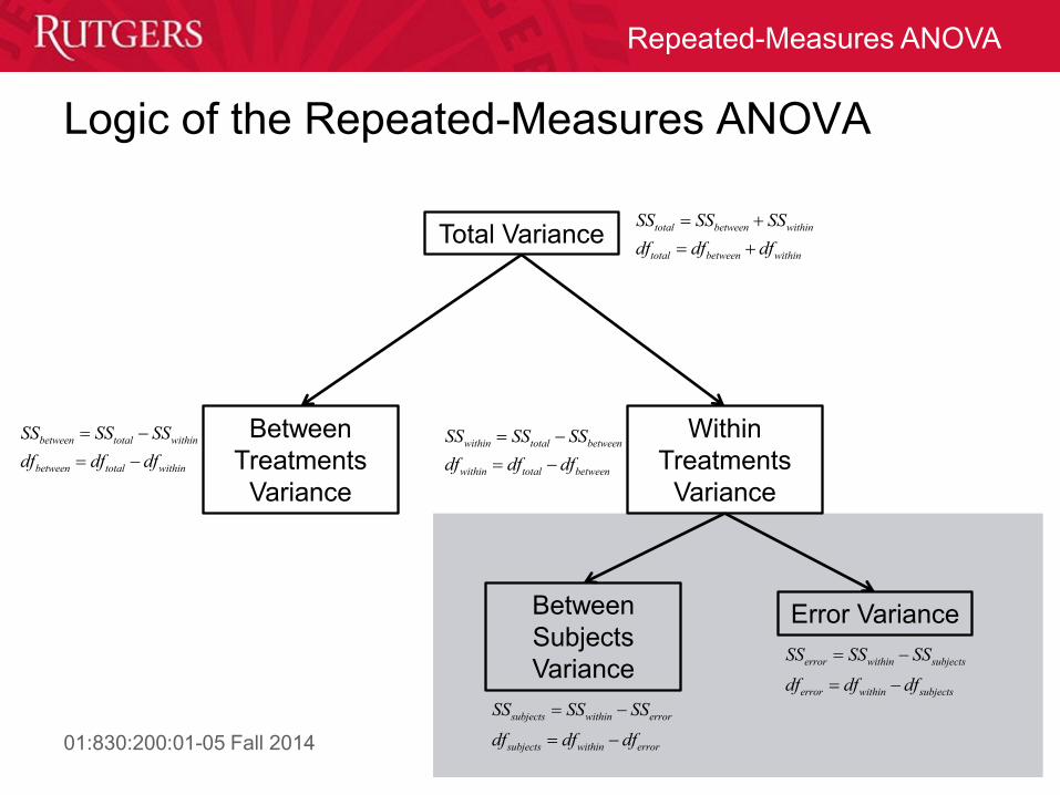
• This is accomplished by a two-stage analysis. In the first
stage, total variability (SStotal) is partitioned into variability
between-treatments (SSbetween) and within-treatments
(SSwithin).
– Individual differences do not appear in SSbetween because the same
sample of subjects serves in every treatment.
– On the other hand, individual differences do play a role in SSwithin
because the sample contains different subjects.
• In the second stage of the analysis, we measure the individual
differences by computing the variability between subjects, or
SSsubjects
• This value is subtracted from SSwithin leaving a remainder,
variability due to sampling error, SSerror
01:830:200:01-05 Fall 2014
Repeated-Measures ANOVA
Total Variance
Between
Treatments
Variance
Within
Treatments
Variance
total between within
total between within
SS SS
d
SS
d dfff
between total within
between total within
SS SS
d
SS
d dfff
within total between
within total between
SS SS
d
SS
dfdff
Between
Subjects
Variance
Error Variance
subjects within error
subjects within error
SS SS
df df
SS
df
error within subjects
error within subjects
SS SS
d
S
df
S
dff
Logic of the Repeated-Measures ANOVA

01:830:200:01-05 Fall 2014
Repeated-Measures ANOVA
• Start by computing and for each group, then
compute:
• Grand total: The overall total, computed over all scores in all
groups (samples)
• Total sum of squared scores: The sum of squared scores
computed over all scores in all groups
k n
T ij
i j
x x
2 2k n
T ij
i j
x x
x 2x
Computations for the Repeated-Measures ANOVA

01:830:200:01-05 Fall 2014
Repeated-Measures ANOVA
• In addition, you will have to compute the sum of scores
(across all k conditions) for each subject and/or the mean for
each subject
Computations for the Repeated-Measures ANOVA
isubjectsubject
k
i
xx
subject
subject
xM
k

01:830:200:01-05 Fall 2014
Repeated-Measures ANOVA
Computations for the ANOVA: SS terms
• SStotal : The sum of squared deviations of all observations
from the grand mean
– Again, not strictly needed for computing the F ratio, but it makes
computing the needed SS terms much easier
2
22
total T
T
T
xxSS x M
N
or
total between withinSSSS SS

01:830:200:01-05 Fall 2014
Repeated-Measures ANOVA
Computations for the ANOVA: SS terms
• SSbetween: The sum of squared deviations of the sample
means from the grand mean multiplied by the number of
observations
• SSwithin: The sum of squared deviations within each sample
2
k
between i T
i
SS n M M
within total betweenSS SSSS 1 2 ...k
within j
j
kSS SS SS SS SS or
or totb aet lween withinSS SSSS

01:830:200:01-05 Fall 2014
Repeated-Measures ANOVA
Computations for the Repeated-Measures ANOVA
• SSsubjects : The sum of squared deviations of the subject
means from the grand mean multiplied by the number of
conditions (k)
• SSerror: The sum of squared deviations due to sampling
error
error within subjectsSS SSSS
2
subjects subject TMSS k M

01:830:200:01-05 Fall 2014
Repeated-Measures ANOVA
Computations for the Repeated-Measures ANOVA
• dftotal = N-1 : – degrees of freedom associated with SStotal
– N is the total number of scores
• dfbetween (dfgroup) = k-1 : – degrees of freedom associated with SSbetween
– k is the number of groups
• dfsubjects = n-1 – Degrees of freedom associated with SSsubjects
– n is the number of subjects
• dferror= dftotal - dfbetween -dfsubjects= N-k-n+1 : – degrees of freedom associated with SSerror

01:830:200:01-05 Fall 2014
Repeated-Measures ANOVA
Computing the F-statistic
betweenbetween
between
SSMS
df
errorerror
error
SSMS
df
, error
er
betweenbetween
ror
MSF df df
MS

01:830:200:01-05 Fall 2014
Repeated-Measures ANOVA
The Repeated-Measures ANOVA: Steps
1. State Hypotheses
2. Compute F-ratio statistic:
– For data in which I give you raw scores, you will have to compute:
• Sample means & subject means
• SStotal, SSbetween, SSwithin, SSsubjects, & SSerror
• dftotal, dfbetween, dfwithin, dfsubjects, & dferror
3. Use F-ratio distribution table to find critical F-value representing rejection region
4. Make a decision: does the F-statistic for your sample fall into the rejection region?
, error
er
betweenbetween
ror
MSF df df
MS
01:830:200:01-05 Fall 2014
Repeated-Measures ANOVA
Repeated-Measures ANOVA: Example
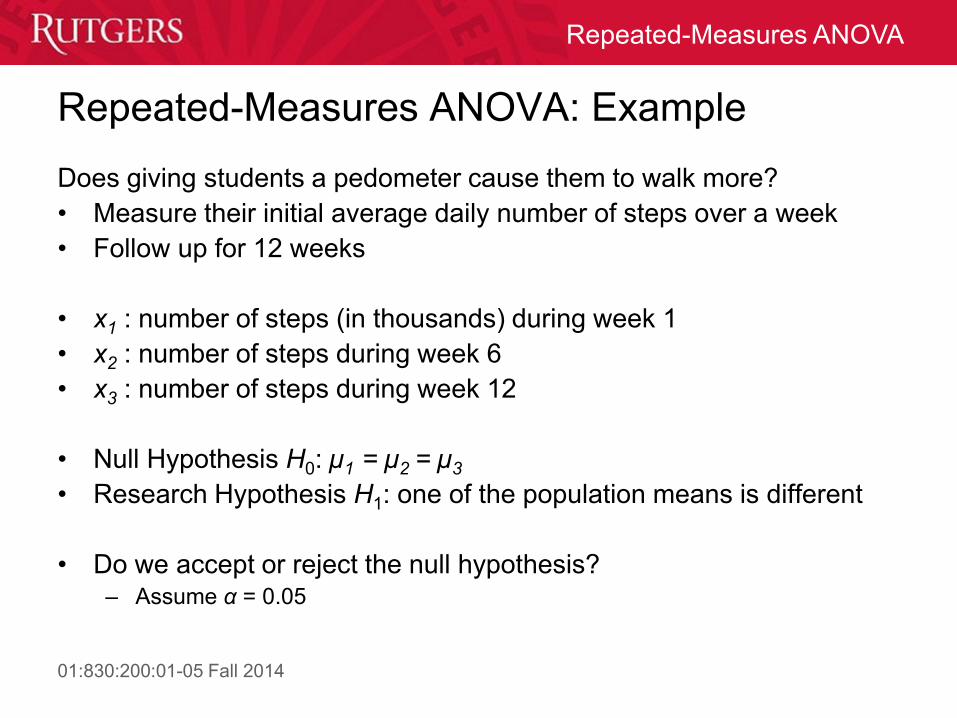
Does giving students a pedometer cause them to walk more?
• Measure their initial average daily number of steps over a week
• Follow up for 12 weeks
• x1 : number of steps (in thousands) during week 1
• x2 : number of steps during week 6
• x3 : number of steps during week 12
• Null Hypothesis H0: µ1 = µ2 = µ3
• Research Hypothesis H1: one of the population means is different
• Do we accept or reject the null hypothesis? – Assume α = 0.05

01:830:200:01-05 Fall 2014
Repeated-Measures ANOVA
Thousands of Steps
Student X1 X2 X3 𝑀𝑠𝑢𝑏𝑗 A 6 8 10 8
B 4 5 6 5
C 5 5 5 5
D 1 2 3 2
E 0 1 2 1
F 2 3 4 3
𝑀𝑔𝑟𝑜𝑢𝑝 3 4 5
112totalSS 4TM
17
21
1 5
10
15
1total
between
within betwee
subjects
total
erro
n
within subje tsr c
df k
d
df N
d
f n
df df df
df f df
Source df SS MS F
Between groups
Within groups
subjects
error
Total 112
Set up a summary ANOVA table:
1. Compute degrees of freedom
01:830:200:01-05 Fall 2014
Repeated-Measures ANOVA
Thousands of Steps
Student X1 X2 X3 𝑀𝑠𝑢𝑏𝑗 A 6 8 10 8
B 4 5 6 5
C 5 5 5 5
D 1 2 3 2
E 0 1 2 1
F 2 3 4 3
𝑀𝑔𝑟𝑜𝑢𝑝 3 4 5
112totalSS 4TM
Source df SS MS F
Between groups 2
Within groups 15
subjects 5
error 10
Total 17 112
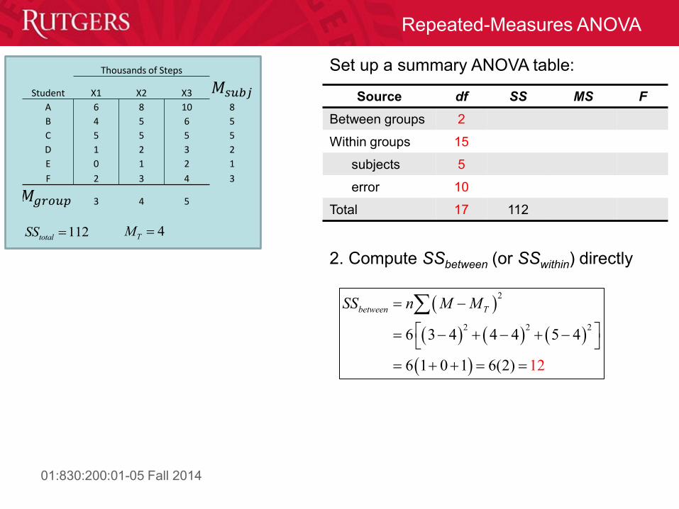
Set up a summary ANOVA table:
2. Compute SSbetween (or SSwithin) directly
2
2 2 26 3 4 4 4 5 4
6 1 0 1 6(2 1) 2
between TSS n M M

01:830:200:01-05 Fall 2014
Repeated-Measures ANOVA
Thousands of Steps
Student X1 X2 X3 𝑀𝑠𝑢𝑏𝑗 A 6 8 10 8
B 4 5 6 5
C 5 5 5 5
D 1 2 3 2
E 0 1 2 1
F 2 3 4 3
𝑀𝑔𝑟𝑜𝑢𝑝 3 4 5
112totalSS 4TM
Source df SS MS F
Between groups 2 12
Within groups 15
subjects 5
error 10
Total 17 112
Set up a summary ANOVA table:
112 02 01 1
within total betweenSS SS SS
3. Compute the missing top-level SS value
(SSbetween or SSwithin) via subtraction
01:830:200:01-05 Fall 2014
Repeated-Measures ANOVA
Thousands of Steps
Student X1 X2 X3 𝑀𝑠𝑢𝑏𝑗 A 6 8 10 8
B 4 5 6 5
C 5 5 5 5
D 1 2 3 2
E 0 1 2 1
F 2 3 4 3
𝑀𝑔𝑟𝑜𝑢𝑝 3 4 5
112totalSS 4TM
Source df SS MS F
Between groups 2 12
Within groups 15 100
subjects 5
error 10
Total 17 112
Set up a summary ANOVA table:
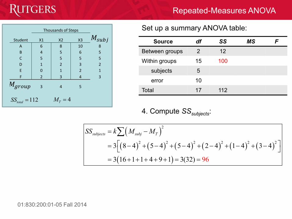
4. Compute SSsubjects:
2
2 2 2 2 2 23 8 4 5 4 5 4 2 4 1 4 3 4
3 16 1 1 94 9 1 3(3 62)
ssub ubj TjectsSS k M M
01:830:200:01-05 Fall 2014
Repeated-Measures ANOVA
Thousands of Steps
Student X1 X2 X3 𝑀𝑠𝑢𝑏𝑗 A 6 8 10 8
B 4 5 6 5
C 5 5 5 5
D 1 2 3 2
E 0 1 2 1
F 2 3 4 3
𝑀𝑔𝑟𝑜𝑢𝑝 3 4 5
112totalSS 4TM
Source df SS MS F
Between groups 2 12
Within groups 15 100
subjects 5 96
error 10
Total 17 112
Set up a summary ANOVA table:
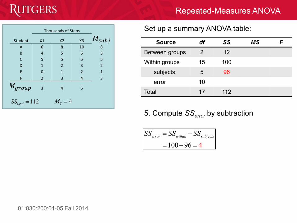
5. Compute SSerror by subtraction
100 96 4
error within subjectsSS SS SS

01:830:200:01-05 Fall 2014
Repeated-Measures ANOVA
Thousands of Steps
Student X1 X2 X3 𝑀𝑠𝑢𝑏𝑗 A 6 8 10 8
B 4 5 6 5
C 5 5 5 5
D 1 2 3 2
E 0 1 2 1
F 2 3 4 3
𝑀𝑔𝑟𝑜𝑢𝑝 3 4 5
112totalSS 4TM
Source df SS MS F
Between groups 2 12
Within groups 15 100
subjects 5 96
error 10 4
Total 17 112
Set up a summary ANOVA table:
6. Compute the MS values needed to
compute the F ratio:
16.0
2
2
betweenbetween
between
SSMS
df
44
10.
0
errorerror
error
SSMS
df

01:830:200:01-05 Fall 2014
Repeated-Measures ANOVA
Thousands of Steps
Student X1 X2 X3 𝑀𝑠𝑢𝑏𝑗 A 6 8 10 8
B 4 5 6 5
C 5 5 5 5
D 1 2 3 2
E 0 1 2 1
F 2 3 4 3
𝑀𝑔𝑟𝑜𝑢𝑝 3 4 5
112totalSS 4TM
Source df SS MS F
Between groups 2 12 6.0
Within groups 15 100
subjects 5 96
error 10 4 0.4
Total 17 112
Set up a summary ANOVA table:
7. Compute the F ratio:
,
6.015.02,10
0.4
betweenbetween error
error
MSF df
MSd
F
f

01:830:200:01-05 Fall 2014
Repeated-Measures ANOVA
1 2 3 4 5 6 7 8 9 10
1 161.45 199.50 215.71 224.58 230.16 233.99 236.77 238.88 240.54 241.88
2 18.51 19.00 19.16 19.25 19.30 19.33 19.35 19.37 19.38 19.40
3 10.13 9.55 9.28 9.12 9.01 8.94 8.89 8.85 8.81 8.79
4 7.71 6.94 6.59 6.39 6.26 6.16 6.09 6.04 6.00 5.96
5 6.61 5.79 5.41 5.19 5.05 4.95 4.88 4.82 4.77 4.74
6 5.99 5.14 4.76 4.53 4.39 4.28 4.21 4.15 4.10 4.06
7 5.59 4.74 4.35 4.12 3.97 3.87 3.79 3.73 3.68 3.64
8 5.32 4.46 4.07 3.84 3.69 3.58 3.50 3.44 3.39 3.35
9 5.12 4.26 3.86 3.63 3.48 3.37 3.29 3.23 3.18 3.14
10 4.96 4.10 3.71 3.48 3.33 3.22 3.14 3.07 3.02 2.98
11 4.84 3.98 3.59 3.36 3.20 3.09 3.01 2.95 2.90 2.85
12 4.75 3.89 3.49 3.26 3.11 3.00 2.91 2.85 2.80 2.75
13 4.67 3.81 3.41 3.18 3.03 2.92 2.83 2.77 2.71 2.67
14 4.60 3.74 3.34 3.11 2.96 2.85 2.76 2.70 2.65 2.60
15 4.54 3.68 3.29 3.06 2.90 2.79 2.71 2.64 2.59 2.54
16 4.49 3.63 3.24 3.01 2.85 2.74 2.66 2.59 2.54 2.49
17 4.45 3.59 3.20 2.96 2.81 2.70 2.61 2.55 2.49 2.45
18 4.41 3.55 3.16 2.93 2.77 2.66 2.58 2.51 2.46 2.41
19 4.38 3.52 3.13 2.90 2.74 2.63 2.54 2.48 2.42 2.38
20 4.35 3.49 3.10 2.87 2.71 2.60 2.51 2.45 2.39 2.35
22 4.30 3.44 3.05 2.82 2.66 2.55 2.46 2.40 2.34 2.30
24 4.26 3.40 3.01 2.78 2.62 2.51 2.42 2.36 2.30 2.25
26 4.23 3.37 2.98 2.74 2.59 2.47 2.39 2.32 2.27 2.22
28 4.20 3.34 2.95 2.71 2.56 2.45 2.36 2.29 2.24 2.19
30 4.17 3.32 2.92 2.69 2.53 2.42 2.33 2.27 2.21 2.16
40 4.08 3.23 2.84 2.61 2.45 2.34 2.25 2.18 2.12 2.08
50 4.03 3.18 2.79 2.56 2.40 2.29 2.20 2.13 2.07 2.03
60 4.00 3.15 2.76 2.53 2.37 2.25 2.17 2.10 2.04 1.99
120 3.92 3.07 2.68 2.45 2.29 2.18 2.09 2.02 1.96 1.91
200 3.89 3.04 2.65 2.42 2.26 2.14 2.06 1.98 1.93 1.88
500 3.86 3.01 2.62 2.39 2.23 2.12 2.03 1.96 1.90 1.85
1000 3.85 3.00 2.61 2.38 2.22 2.11 2.02 1.95 1.89 1.84
dfnumerator
F table for α=0.05
reject H0
df e
rro
r

01:830:200:01-05 Fall 2014
Repeated-Measures ANOVA
Thousands of Steps
Student X1 X2 X3 𝑀𝑠𝑢𝑏𝑗 A 6 8 10 8
B 4 5 6 5
C 5 5 5 5
D 1 2 3 2
E 0 1 2 1
F 2 3 4 3
𝑀𝑔𝑟𝑜𝑢𝑝 3 4 5
112totalSS 4TM
Source df SS MS F
Between groups 2 12 6.0 15.0
Within groups 15 100
subjects 5 96
error 10 4 0.4
Total 17 112
Set up a summary ANOVA table:
8. Compare computed F statistic with Fcrit
and make a decision
015 4.1, r
4.
eject
1critF
H
Conclusion: Giving students pedometers influences the
amount of walking that they do.

01:830:200:01-05 Fall 2014
Repeated-Measures ANOVA
Compute MSbetween , MSerror & F
6
6.0.9
62
70
,
,17
betwewithin
within
enbetween d
MSF df
MS
F
f
16
2
2
betweenbetween
between
SSMS
df
6.67100
15
withinwithin
within
SSMS
df
Note that if we had computed F without
accounting for the repeated-measures
design of the study:
,
2,106
0.415
betwerror
err
eenbetween
or
MSF df
MS
F
df
16
2
2
betweenbetween
between
SSMS
df
44
10.
0
errorerror
error
SSMS
df

01:830:200:01-05 Fall 2014
Repeated-Measures ANOVA
Effect Size for the Repeated-Measures ANOVA
• For repeated-measures ANOVAs, effect sizes are usually
indicated using partial eta-squared
– Partial eta-squared is like the eta-squared that we use to measure effect
sizes in the independent-samples ANOVA, except that it removes the
effect of between-subjects variability
For our example:
2 12.0
16.00.75between between
p
total subject between error
SS SS
SS SS SS SS
2 variability explained by treatment effect
total variability (- subject variability)p
2
p

01:830:200:01-05 Fall 2014
Repeated-Measures ANOVA
Source df SS MS F
Between groups 2 12 6.0 15.0
Within groups 15 100
subjects 5 96
error 10 4 0.4
Total 17 112
Post hoc test: Example (Fisher’s LSD)
ANOVA Summary Table
2
1
3
3
4
5
M
M
M
Let’s do all possible comparisons: {1,2},{1,3},{2,3}
2
error
error error erro
A
r
A B BM M M Mt df
MS MS MS
n n n
Again, note that the denominator is the same for
all comparisons:
1 2 3 6nn n
t-statistic for Fisher’s LSD test
when comparing {A,B}:
102 0.4 0.36
6
5
A B A BM M M Mt

01:830:200:01-05 Fall 2014
Repeated-Measures ANOVA
Level of significance for one-tailed test
0.25 0.2 0.15 0.1 0.05 0.025 0.01 0.005 0.0005
Level of significance for two-tailed test
df 0.5 0.4 0.3 0.2 0.1 0.05 0.02 0.01 0.001
1 1.000 1.376 1.963 3.078 6.314 12.706 31.821 63.657 636.619
2 0.816 1.061 1.386 1.886 2.920 4.303 6.965 9.925 31.599
3 0.765 0.978 1.250 1.638 2.353 3.182 4.541 5.841 12.924
4 0.741 0.941 1.190 1.533 2.132 2.776 3.747 4.604 8.610
5 0.727 0.920 1.156 1.476 2.015 2.571 3.365 4.032 6.869
6 0.718 0.906 1.134 1.440 1.943 2.447 3.143 3.707 5.959
7 0.711 0.896 1.119 1.415 1.895 2.365 2.998 3.499 5.408
8 0.706 0.889 1.108 1.397 1.860 2.306 2.896 3.355 5.041
9 0.703 0.883 1.100 1.383 1.833 2.262 2.821 3.250 4.781
10 0.700 0.879 1.093 1.372 1.812 2.228 2.764 3.169 4.587
11 0.697 0.876 1.088 1.363 1.796 2.201 2.718 3.106 4.437
12 0.695 0.873 1.083 1.356 1.782 2.179 2.681 3.055 4.318
13 0.694 0.870 1.079 1.350 1.771 2.160 2.650 3.012 4.221
14 0.692 0.868 1.076 1.345 1.761 2.145 2.624 2.977 4.140
15 0.691 0.866 1.074 1.341 1.753 2.131 2.602 2.947 4.073
16 0.690 0.865 1.071 1.337 1.746 2.120 2.583 2.921 4.015
17 0.689 0.863 1.069 1.333 1.740 2.110 2.567 2.898 3.965
18 0.688 0.862 1.067 1.330 1.734 2.101 2.552 2.878 3.922
19 0.688 0.861 1.066 1.328 1.729 2.093 2.539 2.861 3.883
20 0.687 0.860 1.064 1.325 1.725 2.086 2.528 2.845 3.850 21 0.686 0.859 1.063 1.323 1.721 2.080 2.518 2.831 3.819
22 0.686 0.858 1.061 1.321 1.717 2.074 2.508 2.819 3.792
23 0.685 0.858 1.060 1.319 1.714 2.069 2.500 2.807 3.768
24 0.685 0.857 1.059 1.318 1.711 2.064 2.492 2.797 3.745
25 0.684 0.856 1.058 1.316 1.708 2.060 2.485 2.787 3.725 26 0.684 0.856 1.058 1.315 1.706 2.056 2.479 2.779 3.707
27 0.684 0.855 1.057 1.314 1.703 2.052 2.473 2.771 3.690
28 0.683 0.855 1.056 1.313 1.701 2.048 2.467 2.763 3.674
29 0.683 0.854 1.055 1.311 1.699 2.045 2.462 2.756 3.659
30 0.683 0.854 1.055 1.310 1.697 2.042 2.457 2.750 3.646 40 0.681 0.851 1.050 1.303 1.684 2.021 2.423 2.704 3.551
50 0.679 0.849 1.047 1.299 1.676 2.009 2.403 2.678 3.496
100 0.677 0.845 1.042 1.290 1.660 1.984 2.364 2.626 3.390
t-Distribution Table
Two-tailed test
One-tailed test
α
t
α/2 α/2
t -t

01:830:200:01-05 Fall 2014
Repeated-Measures ANOVA
Post hoc tests: Example (Fisher’s LSD)
Apply the t-test formula to all comparisons:
1 2100.365
0.36
2.74
5
3 4
0.365
1
M Mt
{1,2} {1,3} {2,3}
2
1
3
3
4
5
M
M
M
1 3100.365
0.36
5.48
5
3 5
0.365
2
M Mt
2 310
0.365
0.36
2.74
5
4 5
0.365
1
M Mt
2.228critt