The Returns to Knowledge Hierarchies�

Luis Garicano Thomas N. Hubbard

London School of Economics Northwestern University

October 21, 2009

Abstract

Hierarchies allow individuals to leverage their knowledge through others�time.This mechanism increases productivity and ampli�es the impact of skill heterogene-ity on earnings inequality. To quantify this e¤ect, we analyze the earnings andorganization of U.S. lawyers and use an equilibrium model of knowledge hierarchiesinspired by Garicano and Rossi-Hansberg (2006) to assess how much lawyers�pro-ductivity and the distribution of earnings across lawyers re�ects lawyers�ability toorganize problem-solving hierarchically. Our estimates imply that hierarchical pro-duction leads to at least a 30% increase in productivity in this industry, relativeto a situation where lawyers within the same o¢ ce do not �vertically specialize.�We further �nd that it ampli�es earnings inequality, increasing the ratio betweenthe 95th and 50th percentiles from 3.7 to 4.8. We conclude that the impact ofhierarchy on productivity and earnings distributions in this industry is substantialbut not dramatic, re�ecting the fact that the problems lawyers face are diverse andthat the solutions tend to be customized.

�We thank Pol Antras, Matthew Gentzkow, Lars Nesheim and Esteban Rossi-Hansberg and partici-pants at various seminars, the 2006 Summer Meetings of the Econometric Society, and NBER SummerInstitute for comments and suggestions. We are especially grateful to Steve Tadelis, who presented thispaper and o¤ered extensive comments at the latter. The research in this paper was conducted while theauthors were Census Bureau research associates at the Chicago Research Data Center. Research resultsand conclusions are those of the authors and do not necessarily indicate concurrence by the Bureau ofthe Census. This paper has been screened to ensure that no con�dential data are revealed.

I. INTRODUCTION

Knowledge is an asset with increasing returns because acquiring it involves a �xed cost,independent of its subsequent utilization. But when knowledge is embodied in individuals,individuals must spend time applying it to each speci�c problem they face and possiblyalso communicating speci�c solutions to others. This makes it di¢ cult for individuals toexploit these increasing returns, relative to a situation where knowledge can be encodedin blueprints, as in Romer (1986, 1990). For example, radiologists who are experts atinterpreting x-rays generally cannot sell their knowledge in a market like a blueprint;instead, they usually must apply their knowledge to each patient�s speci�c x-ray. A wayaround this problem is vertical, or hierarchical, specialization where some non-expertradiologists (e.g., residents) diagnose routine cases and request help from experts in casesthey �nd di¢ cult. Recent work in organizational economics, starting with Garicano(2000), has analyzed how such knowledge hierarchies allow experts to exploit increasingreturns from their knowledge by leveraging it through others�time.What are the returns to �knowledge hierarchies?� In this paper we study this question

empirically in a context where production depends strongly on solving problems: legal ser-vices. We analyze the earnings and organization of U.S. lawyers, and use a model inspiredby the equilibrium model of knowledge hierarchies in Garicano and Rossi-Hansberg (2006)to estimate the returns to specialization that hierarchical production provides lawyers, andthe impact this has on earnings inequality among these individuals.1

We proceed in two stages. We begin in Section II by developing an empirically estimableequilibrium model of hierarchical production, adapting Garicano and Rossi-Hansberg�s(2006) framework to allow for hierarchies with more managers than workers and dimin-ishing returns to managerial span or �leverage� (number of workers per manager). Inthis model, individuals have heterogeneous ability �some are more skilled than others �and hierarchical production allows more talented individuals to leverage their knowledgeby applying it to others� time. Our production function captures the organization ofthe division of labor within hierarchies, which is derived from �rst principles in Garicanoand Rossi-Hansberg (2006), through two assumptions. First, managers who increasetheir span of control must work with higher-skilled workers, since increasing span requiresthem to delegate tasks they previously did themselves. Second, working in a team in-volves coordination costs that do not appear when individuals work on their own. The�hierarchical production function� and equilibrium assignment that result contain twocrucial features that facilitate estimation of the model�s parameters: �rst, the productiv-ity of a hierarchical team, per unit of time spent in production, is determined only by the

1See also Garicano and Hubbard (2007b) for empirical tests of Garicano (2000) that relate law o¢ ces�hierarchical structure to the degree to which lawyers �eld-specialize. Unlike this paper, our previouswork neither examines earnings or assignment patterns nor estimates the returns to hierarchy.

1

manager�s skill; second, the number of workers per manager or leverage is a su¢ cient sta-tistic for worker skill. The �rst of these reduces the empirical problem to estimating thetime cost of hierarchical production, and the second simpli�es our application of hedonictechniques to estimate this cost.We then estimate the parameters of this model using data from the U.S. Economic Cen-

sus on thousands of law o¢ ces throughout the United States. These data contain lawo¢ ce-level information on, among other things, partners�earnings, associates�earnings,and associate-partner ratios. With these parameters in hand, we then use our frameworkto infer the �returns to hierarchy��how much production would be lost if partners werenot able to �vertically specialize�by delegating work to associates, and to construct earn-ings distributions across lawyers, comparing those we observe to those that would obtainif lawyers could not organize hierarchically. We conclude that hierarchical productionhas a substantial e¤ect on lawyers�productivity, raising lawyers�output by at least 30%relative to non-hierarchical production in which there is no vertical specialization withino¢ ces. We also �nd that hierarchies substantially expand earnings inequality, increasingthe ratio between the 95th percentile and median earnings among lawyers from 3.7 to4.8, mostly by increasing the earnings of the very highest percentile lawyers in businessand litigation-related segments, and leaving relatively una¤ected the earnings of the lessleveraged lawyers. Though these e¤ects are reasonably large, we believe them to be farsmaller than in other sectors of the economy. We discuss the source of these di¤erencesand what they may mean for production in the service sector in the paper�s conclusion.We see the contribution of the paper as methodological as well as substantive. Method-

ologically, we wish to reintroduce the idea that the organization of production and earningspatterns within industries are jointly determined by the same underlying mechanism: theequilibrium assignment of individuals to �rms and hierarchical positions. This equilib-rium assignment, in turn, re�ects the characteristics of the underlying production function(Lucas (1978), Rosen (1982)).2 This idea has been underexploited, in part because of thelack of data sets that contain not only information about individuals�earnings, but alsoon their position within their �rms�organization and their �rms�characteristics.3 To ex-ploit these patterns requires combining equilibrium analysis with organizational models.Evidence on who works with whom and in what capacity can be enormously informa-tive, but inferences from such evidence must be based on equilibrium models since suchmodels allow assignments to be based on individuals�comparative rather than absolute

2Rosen notes that �the �rm cannot be analyzed in isolation from other production units in the economy.Rather, each person must be placed in his proper niche, and the marriage of personnel to positions andto �rms must be addressed directly.�(322)

3It might also re�ect an intellectual separation between the �elds of labor economics and industrialorganization that Rosen (1982) was trying to bridge.

2

advantage.Before jumping to our analysis, a few caveats are in order. Our approach, which

emphasizes and exploits labor market equilibria, does not come for free. We largelyabstract from most of the incentive issues that dominate the organizational economicsliterature, as well as many of the details of internal labor markets. We also must placerestrictions on agent heterogeneity so that our equilibrium does not involve sorting onmultiple dimensions. The returns to this approach are considerable, however, as itprovides for a tractable equilibrium model from which we can estimate the impact oforganization (or, equivalently, the impact of vertical specialization) on lawyers�outputand the distribution of lawyers�earnings. In short, this approach allows us to develop a�rst estimate of the returns to hierarchical production.

II. ECONOMIC MODEL: HIERARCHIES, ASSIGNMENT, ANDHETEROGENEITY

II.1. Tastes and Technology

Building on Lucas (1978), Rosen (1982), and Garicano and Rossi-Hansberg (2006)(hereafter, GRH), we develop a general hierarchical assignment model and characterize itsequilibrium properties. Our model is based on a hierarchical production function where,like in these earlier papers, managerial skill raises the productivity of all the inputs towhich it is applied.We assume that demand for a service Z can be described by the demand of a mass of

representative agents with semilinear preferences. We specify:

U = u(z) + y

where u(z) is the utility attained from the consumption of quality z 2 [0; 1] of the serviceZ and y is the utility (in dollars) obtained from the rest of the goods in the agent�sconsumption bundle. We assume u0(z) > 0, and u(0) = 0. Each agent maximizesutility subject to a budget constraint v(z) + y = Y , where v(z) is the cost (in dollars) ofpurchasing a level z of service Z.Suppliers are endowed with a skill level z 2 [0; 1] and with one unit of time. That is they

can supply up to quality level z costlessly and above that level at an in�nite cost. Thepopulation of suppliers is described by a distribution of skill, �(z); with density function� (z). Production of the service Z involves the application of individual suppliers�skilland time to production. An agent with skill z can provide a quality z of Z working onhis own. This has a value in the market of v(z); this value v(z) is an equilibrium object

3

that we characterize below.Following GRH, z can be thought of in our empirical context as an index that re�ects

the share of client problems in a particular �eld that a lawyer working in this �eld cansolve: more-skilled lawyers can solve a greater share of these problems than less-skilledlawyers, and the problems that a less-skilled lawyer can solve are a subset of those that amore-skilled lawyer can solve.To �x ideas, consider the output of a set of suppliers who are each working on their

own, n of whom have skill zw, 1 of whom has skill zm. Total output for these n+1 agentswould be v(zm) + nv(zw). Below we will compare output in this case with output whenagents are allowed to organize hierarchically. This comparison will both illuminate thebene�ts and drawbacks of hierarchical production, and will convey the central challengein estimating the returns to hierarchy.

Hierarchical Production.�Agents may work on their own or as part of a hierarchical team. Following Lucas (1978),

Rosen (1982), and GRH, we propose that hierarchical production allows one individual�sskill to be applied to other individuals�time. The �skill�of a hierarchical team is thereforeequal to the maximum skill available in the team, and output is equal to the value of thisskill multiplied by the time the team spends in production. We thus specify the outputof a team with one individual (the �manager�) with skill zm and a measure of n workerswith skill zw as:

F (zm; zw) = v(maxfzm; zwg)g(n)

We make two key assumptions about this production function.

Assumption 1: Costly Coordination. Production is increasing in team size, g0 > 0:Coordination costs imply that time spent in production is less than the team�s timeendowment, g(n) < n+ 1:

Hierarchical production is thus costly in terms of time: it allows an agent�s skill to beapplied to others�time, but time is expended in the process. Thus g(n) is the team�s�e¤ective time� in production, where g(n) is a mapping from the team members�timeendowment n+ 1 to �e¤ective time.�Our empirical analysis will assume that g(n) = (n + 1)�; 0 < � < 1, so that n units

of worker time and 1 unit of manager time results in (n + 1)� units of time spent inproduction. � is a returns to scale parameter, in this case capturing the returns to scaleassociated with managerial leverage. However, our analytical approach does not dependon this particular speci�cation of g(n).

4

Assumption 2. Span of Control and Worker Skill. The measure of workers n withwhom a manager can work is positive and increasing in the skill of the workers zw:

n(zw) > 0 and n0 (zw) > 0 for all zw:

This assumption captures the idea that managers�time is limited, but managers areable to delegate more di¢ cult tasks to more-skilled workers. Time-constrained managerswho wish to scale up must delegate to workers tasks that they used to do themselves,and this requires them to work with more-skilled workers. The greater the skill of theworkers, the less help each worker needs, and the more workers the manager can have inhis or her team.4

From Assumptions 1 and 2, it is immediate that it is never optimal to have zm < zw,and thus we can rewrite our hierarchical production function, without loss of generality,as:

F (zm; zw) = v(zm)g(n(zw))

The trade-o¤ associated with hierarchical production is now evident. Figure 1 illus-trates output under hierarchical and non-hierarchical production, in the problem solvingvariant, in which g(n) = (n+1)�. The top of Figure 1 depicts nonhierarchical production,in which agents work on their own. The left side of this panel depicts the skill of n + 1agents. The lines depict these agents�time endowments, the shaded regions depict theseagents�skill, or problem-solving ability. n of these agents have skill zw, 1 has skill zm.Assume that each of these agents confronts a set of problems that vary in their di¢ culty,and that each of these sets requires one unit of agent time to handle. These n+1 sets ofproblems are depicted by the thin bars on the right. Under nonhierarchical production,each of these agents simply handles the problems they themselves confront. The value ofthe output of each of the n lower-skilled agents would be v(zw) and value of the outputof the higher-skilled agent would be v(zm). Total output would be v(zm) + nv(zw).The bottom part of this Figure depicts hierarchical production. Total output is

v(zm)(n + 1)�, the product of the value of the manager�s skill and the time the n + 1

agents spend directly in production. Output per unit of productive time is improved,relative to autarchic production, because managers can apply their knowledge to morethan one set of problems. This improvement is the bene�t of hierarchical production;

4Although we state this assumption in general terms, it is straightforward to generate it from �rstprinciples in a more speci�c framework. In Garicano (2000) and GRH, workers draw problems and askfor help from managers whenever they cannot solve it. Assuming that the probability that a workerneeds help is 1 � zw, the number of workers a manager can help is determined by his time constraint(1� zw)hn = 1; where h is the per-problem time cost of helping, resulting in n0(zw) > 0:

5

the drawback is that hierarchical production involves a loss in time spent in production.The Figure also illustrates the empirical task we will confront when estimating the

returns to hierarchy. Our goal is to compare realized production and earnings to whatproduction and earnings would be, absent hierarchical production. Our data will containinformation on F (zm; zw), law o¢ ces�output, and n, law o¢ ces�associate-partner ratios.It follows that if � were known, one could infer v(zm) �what partners would earn, absenthierarchical production �because v(zm) = F (zm; zw)=(n + 1)�. Much of our empiricalfocus will therefore be aimed at estimating �, or more broadly the time cost associatedwith hierarchical production.5

Production in most contexts, even human capital intensive contexts like ours, involvesinputs other than individuals�knowledge. We allow for this by introducing �overhead�inputs into the model in the following way.

Assumption 3: Monotonic and convex overhead costs Overhead and other costs(e.g., for o¢ ce space, support sta¤) are positive, increasing, and weakly convex inteam size, c(n+ 1) > 0; c0(n+ 1) > 0; c00(n+ 1) � 0:

II.2. Equilibrium

Stochastic Elements.�Our estimation framework will rely on two key equilibrium relationships: a �rst or-

der condition characterizing managers� optimal choice of workers, and the equilibriumrelationship between an associate�s earnings w and the associate-partner ratio n at theassociate�s o¢ ce. Utilizing these relationships empirically requires us to introduce sto-chastic elements into the model in a way that makes the structure of these relationshipswell-de�ned but not deterministic. We therefore make the following assumptions.

Assumption 4: Stochastic productivity. The productivity of teams is stochastic, sothat the value of production at o¢ ce i per unit of productive time is: vi(zm) =v(zm)"i where "i is i.i.d., "i > 0, E("i) = 1. Productivity shocks are realized afterorganizational decisions are made, so that they a¤ect partners�earnings but not theorganizational equilibrium. These shocks a¤ect the team�s rate of output during

5F (zm; zw) is closely related to production functions that have been applied elsewhere in the literatureon hierarchical sorting. The production function in Lucas (1978) can be written as F (zm; zw) = zmg(n);and thus represents a special case of our model in which the skill of workers is irrelevant, and only theskill of managers matters. A two-layer version of the production function in GRH can be obtained fromF (zm; zw) by specifying v(z) = z, n(z) = 1=(h(1� z)), and g(n) = n for n > 1. (Other elements of GRHare more general than our model; they allow for hierarchies with more than two layers, and allow theskill distribution among agents to be endogenous. We make fewer assumptions about the nature of theinteraction between managerial and worker skill than GRH, but do not derive hierarchical productionfrom �rst principles as they do.)

6

time in production.6

Assumption 5: Compensating di¤erentials. Agents have preferences with respectto working as associates under di¤erent partners, so that the wage that a partnerat o¢ ce i must pay to compensate associates at the o¢ ce by an amount w equalswi = w�i, where �i > 0, E(�i) = 1; and �i is an absolutely continuous i.i.d. randomvariable, and is independent of all variables in the model.

An important element of Assumption 4 is that productivity is realized after the orga-nizational equilibrium is obtained; we view this as reasonable in our empirical context,in which there is a distinct season for hiring associates and where some of the details ofproduction (e.g., how time-intensive it is to communicate solutions to particular clients)are unknown at the time associates are hired.Assumption 5 implies that any nonwage amenities of working as associates at o¢ ce i

are valued the same across individuals, and that this value is independent of the o¢ ce�sassociate-partner ratio and, for that matter, the skill of the partners.7 These conditionsare necessary to keep the labor market equilibrium tractable because they will implythat any systematic sorting between agents is by skill and not other dimensions. Thisrules out multidimensional sorting, but is obviously stringent, in particular in this contextbecause the independence assumption rules out the possibility that associates are willingto work for less under higher skilled partners than lower-skilled partners (perhaps forreasons having to do with training or client contacts). We will discuss the direction andmagnitude of biases introduced by this assumption below.

Output Market.�By the representative agents��rst-order conditions, the price schedule in the output

market is given by the value schedule of the representative consumer: u0(z) = v0(z) subjectto u(z) � v(z): To simplify, we assume that the mass of demanders exceeds the capacityof suppliers. Under this assumption, the price schedule that solves this problem is givenby the utility of the representative consumer, that is:

v(z) = u(z)

Trivially, this implies a price schedule where v0(z) > 0 and v(0) = 0.

6Note that this is distinct from the coordination cost �, which re�ects time loss from working withothers. Individuals optimize knowing �. Furthermore, productivity is stochastic at all o¢ ces, includingo¢ ces where individuals work on their own.

7This is the standard compensating di¤erentials assumption. With homogeneous agents, the equilib-rium wage is such that individuals are indi¤erent between the di¤erent amenities: the wage "equalizes"utilities (see e.g. Rosen (1986)). Note also that individuals have the same preferences with respect toworking as an associate at o¢ ce i. This makes the equilibrium analysis simpler than in hedonic labormarket models where workers di¤er in their preferences.

7

Labor Market.�Like in GRH, the continuum of heterogeneous agents make occupational choices and

team composition choices to maximize their compensation given the price schedule v(z).8

Each agent chooses whether to be a manager, to work on their own, or be a worker, andearn in expectation R, v(z), or w(z), respectively, where w(z) relates the compensationan agent receives as a worker to the agent�s skill. w(z) is a hedonic wage function equatesthe supply and demand for skill at each skill level, and is thus an equilibrium object.The labor market equilibrium involves solving a continuous assignment problem. The

production function is continuous and involves complementarities between worker andmanager skill, @2F (zm; zw)=(@zm@zw) > 0: Thus in general the assignment exists, is oneto one in terms of skill, and is unique (Chiappori, McCann and Nesheim, forthcoming).9

Thus there exist a matching function zm = m(zw) derived from the equality of supply anddemand for skill at each point that maps the skill of workers to the skill of their managers.R, the residual earnings (or �rents�) of a manager of skill zm who has hired n workers

of skill zw, can be written as:

R = "iv(zm)(n(zw) + 1)� � win(zw)� c(n(zw) + 1) (1)

The �rst term is the value of output; in our context, the revenues associated with a partnerand his or her associates. The second term is the wage cost of hiring n associates of skillzw: The third term is the overhead cost associated with the partner and associates.Agents evaluate R at the point where they have chosen the skill level of their workers

to maximize expected earnings, given the wage schedule they face wi = w(zw)�i. Thisimplies a �rst order condition:

v(zm)�(n(zw) + 1)��1n0(zw)� w0i(zw)n(zw)� wi(zw)n0(zw)� c0(n+ 1)n0(zw) = 0

Given zm = m(zw), the above equation is a di¤erential equation in w(z); all the otherobjects are given. Assumption 2, combined with the fact that worker skill only enters theproduction function through managerial leverage, implies that managerial leverage n isan invertible function of worker skill zw. Because of this, the labor market equilibriumcan be equivalently characterized in terms of the supply and demand for leverage, n. The

8Compensation for agents who choose to be workers, w, includes any compensating di¤erential.9Speci�cally, Chiappori, McCann, and Nesheim (forthcoming) show that assignments in a class of

problems including ours (e.g. including the possibility that some agents will not participate in themarket) exist with great generality and that under a generalized Spence-Mirrlees condition (of which ourpositive cross-derivative is a special case), the assignments are unique and one-to-one outside a negligibleset.

8

�rst order condition above can be restated as:

v(zm)�(n+ 1)��1 = w0i(n)n+ wi(n) + c

0(n+ 1) (2)

and the hedonic wage function can be stated instead in terms of n, w(n) and itsderivative w0(n).10 This condition holds in equilibrium for all individuals who choose tobe leveraged managers, and summarizes these agents�demand for leverage. As appliedto our context, lawyers�choice of n is greater, the greater their skill, zm, and the lower�i: higher skill makes leverage more valuable, and lawyers with lower �i can obtain it atlower cost. The fact that n is an invertible function of worker skill means that similarrelationships hold when looking at worker skill: lawyers with higher zm and lower �ichoose to work with more skilled, as well as more, associates. In equilibrium, there willbe systematic sorting between lawyers on the basis of skill, but not on other characteristicsgiven that lawyers, and in particular lawyers who choose to work as associates, are assumedto have the same preferences for nonwage amenities as captured by �i.An empirical advantage of reformulating the problem in terms of the supply and de-

mand for leverage rather than the supply and demand for skill is that n is a variablewe observe directly in the data �it is the number of associates per partner. This makesthe �rst order condition more useful for estimation purposes, because we have eliminatedan unobservable variable. It also helps with respect to utilizing hedonic techniques inrecovering w(n). A common problem that researchers encounter when utilizing hedonictechniques to recover supply or demand parameters is sorting on unobservables; absentthis reformulation, we would face this problem as well, because we do not observe skillwithout error (in fact, we do not observe it at all). Given the assumptions of our model,this is not an issue here: because there is no systematic matching between partners andassociates on characteristics other than skill, there is no problem associated with sortingon unobservables �we observe a su¢ cient statistic, n, which summarizes all relevant as-pects of skill, including both that which is captured in usual proxies and that which isnot.11 The invertibility property means that the quantities n and w

0(n) summarize a lot

of information in equilibrium. n is not only the number of workers per manager, but isalso an error-free index of workers�skill.12 Likewise w

0(n) is not only the marginal price

10We are abusing notation slightly here, as w(n) and w(z) are di¤erent functions. w0i(n) in this equationis dwi(n)

dn .11Our exploitation of the invertibility of n(z) is similar to Olley and Pakes�(1995) use of the invertibility

of the investment function in productivity estimation. In both cases, the idea is that if theory implies thatan agent�s decision variable increases monotonically with an unobserved variable, an arbitrary increasingfunction of the decision variable substitutes for the unobserved variable.12Note that this is true under a wide variety of additional assumptions that might change the wage

schedule or the match between associates and partners, but not the invertibility of n(z). For example,if more skilled associates are willing to work for less for more skilled partners, n would continue to be a

9

of leverage, but is also a monotonic transformation of the marginal price of skill.Using the de�nition of R and the production function F (zm; zw) = "iv(zm)(n+ 1)�, we

can rewrite the �rst order condition as:

F (zm; zw)

n+ 1| {z } � 1"i = w0in+ wi + c0| {z } (3)

Average Revenues �1

"i= Marginal Cost

The left side of this equation is the marginal bene�ts of leverage, which are the averagerevenues per team member multiplied by �="i; the right is the marginal cost of leverage.This marginal cost contains three terms: the extra wage that needs to be paid to all teammembers w0i (increasing leverage requires better as well as more workers), the wage of theadditional agent, and the additional overhead cost. Thus the equilibrium relationshipcan be rewritten as:

� =MC

AR"i (4)

or:lnAR� ln[w0i(n)n+ wi + c0(n+ 1)] = � ln � + ln "i (5)

Our estimates of � are based on this equation. Identi�cation of � is based on a straightfor-ward idea that has been applied many times in the context of estimating returns to scale.In equilibrium, each manager chooses n such that the marginal bene�ts to leverage equalthe marginal cost of leverage. If there are constant returns to leverage �� = 1 �thenthe average bene�ts of leverage equal the marginal bene�ts of leverage, and therefore theaverage bene�ts of leverage should equal the marginal cost of leverage. Finding that thisis not the case �in particular, that the average bene�ts of leverage exceed the marginalcost of leverage � is evidence that there are decreasing returns to leverage, and underour speci�cation the ratio between the marginal cost and the average bene�ts of leverageindicates the magnitude of decreasing returns.The left side of this equation contains four terms: revenues per team member, the

marginal price of leverage, worker pay, and the marginal overhead cost associated withworkers. As we describe in further detail below, we obtain estimates for the marginal priceof leverage from the coe¢ cients in the hedonic wage regression implied by Assumption5.13

su¢ cient statistic for associate skill, since this would merely reinforce positive sorting.13We also explain below how we construct estimates of c0, the marginal overhead cost. We defer this

discussion because it relies on our data and institutional context, which we describe in the next section.

10

Dynamics and w0(n).�An important assumption in the model is that agents maximize their current-period

compensation, given their skill. This speci�cation of agents�objective, along with As-sumption 5, ensures that agents face a schedule for the marginal price of leverage, w0i(n)that is independent of their skill and therefore the hedonic regression described abovereveals this schedule. However, this rules out dynamic aspects of the labor market, in-cluding that individuals value working with higher-skilled agents because it provides themfuture bene�ts, for example in the form of better training or contacts. Such dynamicaspects are very realistic in our context, but are di¢ cult to incorporate directly in ourmodel and estimation procedure. We can, however, analyze how our estimates wouldchange if our assumption that agents maximize current period earnings were replacedby one in which agents working as associates place an additional value on working withhigher-skilled partners.If we have misspeci�ed agents� tastes in this way, this will tend to bias downward

our estimates of w0i(n), and thus the marginal cost of leverage MC(n), and thereforeultimately �, the coordination costs associated with hierarchy. If associates are willingto work for less for higher-skilled partners, then our estimate of w0i(n) will understate themarginal price of leverage faced by each individual partner; a partner of a given skill will�nd it more expensive to increase leverage because it will cost him more at the margin tooutbid a slightly-higher-skilled partner for a slightly-higher-skilled associate. Estimatesof w0i(n) based on the hedonic regression described above will then be too low. If so, thiswill lead our estimate of �, which is identi�ed by the ratio of marginal cost and averagerevenues, also to be biased downward. This, in turn, will lead us to underestimate thereturns to hierarchy, since a too-low � implies that we overstate the extent to which thepotential returns to hierarchy are eaten up by coordination costs. Our estimates shouldtherefore be treated as a lower bound in this light.We discuss the quantitative impact this has on our estimates below. To preview, our

investigations lead us to believe that leads to only a small bias on our estimates of thereturns to hierarchy.Relatedly, while our analysis largely abstracts from the details of internal labor markets,

there is an issue of whether this abstraction leads us to misestimate the marginal cost ofleverage, and hence �. In particular, one can imagine a multi-period model inspired bytournament theory in which part of the marginal cost of an associate is a prize paid byincumbent partners to the most promising associates in the form of a transfer they receivefrom incumbent partners upon promotion. If this is the case, our analysis understates themarginal cost of leverage, and hence our estimates of the returns to hierarchy are a lowerbound by the same logic as above. We think this perspective is incomplete, however,because characterizing promotions as a cost to incumbent partners ignores the prospec-

11

tive client-generation-related bene�ts of promoting promising lawyers. From incumbentpartners�perspective, it is probably not a cost to promote lawyers who are expected tobe at least as productive as existing partners.14 If so, the promotion-related �prize�thataccrues to the most promising associates should not be considered part of the marginalcost of leverage.

III. DATA AND ESTIMATION

III.1. Data

The data are from the 1992 Census of Services. Along with standard questions aboutrevenues, employment, and other economic variables, the Census asks a large sample oflaw o¢ ces questions about the number of individuals in various occupational classes thatwork at the o¢ ce and payroll by occupational class. For example, it asks o¢ ces to reportthe number of partners or proprietors, the number of associate lawyers, and the number ofnonlawyers that work at the o¢ ce. It also asks payroll by occupational class: for example,the total amount associate lawyers working at the o¢ ce are paid. These questions elicitthe key variables in our analysis. Other questions ask o¢ ces to report the number oflawyers that specialize in each of 13 �elds of the law (e.g., corporate law, tax law, domesticlaw) and the number of lawyers who work across multiple �elds. These variables allow usto control for the �eld composition of lawyers at various points in our analysis. Our mainsample includes 9,283 law o¢ ces. This includes only observations in our sample thatare legally organized as partnerships or proprietorships, because partners and associatesare broken out separately only for these observations.15 Throughout our analysis we usesampling weights supplied by the Census to account for the likelihood each was sampled.These data have several aspects that lend themselves to an analysis of equilibrium as-

signment. They cover an entire, well-de�ned human-capital-intensive industry in whichorganizational positions have a consistent ordering across �rms, and allow us to constructestimates of individuals� earnings at the organizational position*o¢ ce level at a largenumber of �rms. Data that allows one to connect individuals�earnings with �rm char-

14Levin and Tadelis (2005) propose that partnerships�pro�t-sharing aspects provide incumbent partnersan incentive to only add new partners that raise the partnership�s average skill level.15Other o¢ ces are legally organized as "professional service organizations," or "PSOs." As we discuss at

length in Garicano and Hubbard (2007b), it is unlikely that our use of only �rms organized as partnershipsor proprietorships in our main analysis leads to any important sample selection. States began to allow law�rms to organize as PSOs mainly to allow partners the same tax-advantaged treatment of fringe bene�tsas employees of corporations, but this form had few other e¤ects; it remained the case that shareholdersconsisted only of lawyers in the �rm, and that there were no retained revenues. Selection of �rms intothis form as of 1992 largely re�ected when the �rm�s state allowed for PSOs, and not di¤erences in �rmcharacteristics; PSOs were more much common in early-allowing states such as Florida than late-allowingstates such as New York, but their prevalence varied little with their size. In 1992, PSOs made up aboutone-third of the industry in terms of lawyers, o¢ ces, and revenues.

12

acteristics across �rms is not common, and it is even less common to be able to connectearnings with individuals�organizational position. These data have shortcomings, how-ever: in particular, they do not directly report partners�earnings, and thus we have toestimate them from the data at hand.

Estimating Partners�Earnings.�Partnerships commonly pay out to partners their earnings net of expenses during the

year. Thus, earnings per partner at o¢ ce i, Ri, can be depicted by the identity:

Ri = (TRi � winipi � xili � ohi)=pi

where TRi is total revenues at o¢ ce i, wi is average associate earnings at o¢ ce i, ni isassociates per partner, pi is the number of partners, xi is non-lawyer earnings per lawyer,li = pi(1 + ni) is the number of lawyers, and ohi is overhead. This can be rewritten as:

Ri + ohi=pi = (TRi � winipi � xili)=pi

Our data on partnerships contain the variables on the right side of this expression.Thus, we observe the sum of partners�earnings and overhead. We do not observe Ri andohi separately for partnerships; our task is to distinguish between these.To do this, we utilize observations of law o¢ ces that are legally organized as �profes-

sional service organizations,�or �PSOs.� The data the Census collects for these o¢ cesdi¤ers from those the Census collects for partnerships. The Census collects data only onthe total number of lawyers at these o¢ ces �and not separately the number of partnersand associates. This makes these observations unusable in our main analysis, and thusthey are not part of our main sample. However, it collects data on the total pay tolawyers �and not just to associates �which makes these observations useful for analyzingthe determinants of law o¢ ces�overhead. The above identity implies:

ohi = TRi � (Ripi + winipi)� xili

The observations of PSOs contain each of the three terms on the right hand side �revenues,lawyer pay, and nonlawyer pay �and thus allow us to infer overhead for each of theseo¢ ces. We estimate the relationship between overhead and �rm characteristics at PSOs,then use our estimates to obtain overhead estimates at the partnerships in our mainsample; by the identity above, this implies estimates of partners�earnings.

Estimating Overhead.�Our procedure for estimating overhead relies on knowledge of the structure of law �rms�

13

costs, derived mainly from reports on law o¢ ces from the Census�Operating ExpensesSurvey16 and from Altman Weil�s 1994 Survey of Law Firm Economics. In particular,our procedure is mindful of the following:

� �Non-payroll fringe bene�ts�such as health insurance and retirement plan contri-butions are consistently about 15% of payroll.

� Operating expenses increase with the o¢ ce�s scale, some elements with the numberof people in the o¢ ce and some with the amount of business.

For example, rent increases with the number of people. Many of the expenses thatincrease with the amount of business, such as o¢ ce supplies, communications, and expertservices are �pass-through�expenses which are billed through to clients but will appear asboth expenses and revenues in our data. This occurs, for example, when patent lawyershire engineers.

� Some operating expenses such as rent tend to be higher in larger markets.

� O¢ ces�cost structure might di¤er depending on whether they serve businesses orindividuals (e.g., the former might involve more travel or business developmentexpenses). The relationship between overhead and revenues might vary across�elds because �pass-throughs�are more important in some than others (e.g., patentlaw).

We incorporate the �rst of these by simply assuming that fringe bene�ts are 15% ofpayroll for all o¢ ces, which allows our data to be used to explain variation in oh�i = TRi�1:15 � [(Ripi + winipi)� xili]. We incorporate the rest by specifying oh�i as a function ofmarket size, revenues, and the number of individuals working at the o¢ ce (�employment�),interacting market size and employment to allow for the fact that additional o¢ ce spacemay be more costly in larger markets. Furthermore, we allow the relationship betweenrevenues and overhead to vary across �elds.We report the coe¢ cient estimates from this speci�cation in Table 1.17 We allow the

intercept term to vary with indicator variables that correspond to the employment size

16Bureau of the Census (1996).17We included [employment-2] rather than employment in these regressions. Our sample only contains

observations of o¢ ces with positive employment, thus the smallest o¢ ce in our sample has two individuals:a lawyer plus a non-lawyer. This normalization allows us to interpret the intercepts in terms of the �xedcost of operating a very small o¢ ce.The error term in the OLS regression is heteroskedastic; the variance of the residual is higher for

higher-revenue o¢ ces. We therefore use a GLS estimator to correct for this. The �rst stage regressesthe logged square of the residual on a fourth-order polynomial of logged revenues. We use the predictedvalues of this regression as weights in the regression we report here.

14

of the county in which the o¢ ce is located, and include interactions between employmentand these market size measures. The coe¢ cient estimates imply that the �xed overheadcost of a very small law o¢ ce is on the order of $28,500. The interactions suggest that theoverhead associated with each additional individual is about $2,900 in very small countiesbut this tends to be much greater in very large markets. We allow the coe¢ cient onrevenues to enter quadratically and to di¤er across �elds. The estimates indicate thatthe relationship is concave for most �elds, and strongest for patent, banking, and realestate law. The estimates imply that overhead increases by $0.10-$0.25 with each $1.00increase in revenues for most o¢ ces in our sample.The R-squared for this regression, 0.70, is high. We found that more detailed speci�ca-

tions, including those that include county �xed e¤ects instead of the market size dummiesand that interact �eld shares with the employment variables, increase the R-squared byvery small amounts and generate almost exactly the same distributions in lawyers�earn-ings as those reported later in this paper.18

We use these estimates in several ways. We use them to construct estimates of partnerearnings at partnerships. This involves substituting in our estimate for ohi, and de�atingTRi by our estimate of overhead�s share of revenues at each o¢ ce, @ohi=@(revenuesi) fromthe regression coe¢ cients in Table 1. The latter accounts for the fact that some shareof an o¢ ces revenues as reported in our data are pass-through expenses. In Table A1in the Appendix, we show that the distribution of earnings that this procedure generatesclosely matches the distribution of earnings of privately-practicing lawyers from the 1990PUMS data (up until the point at which earnings in the PUMS data are top-coded). Tokeep language simple, we will refer to the partner earnings generated by this procedureas �partner earnings�rather than �estimated partner earnings,�even though the latter ismore accurate.We also use them to construct estimates of c0(n + 1) at each law o¢ ce. With respect

to the latter, we specify:c0(n+ 1) = xi + oh

0i=pi

c0(n + 1) has two parts. One is that hiring an associate requires hiring support sta¤as well; we assume that it requires hiring a proportionate amount of support sta¤, whichimplies an increase in nonlawyer pay of xi. The other part is the increase in overheadper partner. This increase includes an increase in fringe bene�ts �15% of the additionallawyer and nonlawyer payroll associated with hiring an associate. It also includes theincrease in space, computer equipment, etc. that goes along with increasing the employ-

18This likely re�ects that (a) the cost of o¢ ce space varies little across most counties, and (b) therelationship between operating expenses and employment �which largely re�ects costs associated witho¢ ce space, furniture, computer equipment, etc. � indeed should not vary depending on the details ofwhat a law o¢ ce does.

15

ment size of the o¢ ce. We use the coe¢ cients on employment in the overhead regressionto estimate this for every o¢ ce, remembering that the employment increase that comeswith hiring an additional associate includes a proportionate amount of additional supportsta¤ as well.

Summary Statistics and Patterns in the Data.�Median earnings across all lawyers in our main sample are $77,000. The 25th and

75th percentiles are $44,000 and $141,000, respectively. The 95th percentile is about$350,000; there were about 435,000 privately-practicing lawyers in the U.S. in 1992, sothis represents the earnings of roughly the 20,000th-ranked lawyer. About 40% of lawyersare associates, 25% are unleveraged partners (partners in o¢ ces with no associates), and35% are leveraged partners. Among the latter, less than one-half work in o¢ ces with anassociate-partner ratio greater than one.Much of our analysis will be conducted from the perspective of partners�optimal choice

of leverage; it is thus useful to report some statistics from the perspective of the averagepartner in our sample. The �rst column in Table 2 reports that average revenues perpartner were $361,000, and average partner pay was $150,000. On average, partnershad 0.6 associates, to whom they paid $36,000. The average partner worked in ano¢ ce with 15 partners. In light of important ways in this industry are segmented (seeGaricano and Hubbard (2007b)), we classify o¢ ces in the following way. We de�ne�litigation�o¢ ces as those with at least one lawyer specializing in a litigation-intensive�eld (negligence, insurance), and classify the remainder as �business, non-litigation�and�individual, non-litigation�depending on whether the o¢ ce�s primary source of revenuesis from businesses or individual clients. Table 2 indicates that the partners in our sampleare evenly distributed across these three classes of o¢ ces.The second and third columns, which report these averages separately according to

whether o¢ ces have at least one associate, indicate that the averages in the �rst columnmask a lot of variation in our sample. O¢ ces with at least one associate are much largerin terms of the number of partners than those with no associates. Revenues per partnerand partner pay are much higher as well. Our empirical analysis will revolve aroundrelationships between earnings and o¢ ces�hierarchical organization; this table highlightsthe importance of accounting for di¤erences in o¢ ces�scale and lawyers��elds (or theiro¢ ce�s segment), both of which are correlated with both lawyers�earnings and hierarchicalstructure.In other work (Garicano and Hubbard (2007a)), we have investigated earnings and or-

ganizational patterns in these data using a series of regressions. We found that controllingfor lawyers �elds, the size of the local market in which they work, and other variables, (a)partners�earnings and associates�earnings are positively correlated, (b) partners�earnings

16

are higher in o¢ ces where associate-partner ratios are greater, and (c) associate earningsare greater in o¢ ces where associate-partner ratios are greater. These patterns are con-sistent with the hypothesis that manager skill, worker skill, and the worker-manager ratioshould move together. We also investigate how earnings vary with lawyers�position. Wefound that, throughout most of our data and controlling for �eld and local market size, as-sociates earn less than unleveraged lawyers, who in turn earn less than leveraged partners.Furthermore, we found that associates earn less than unleveraged partners, even whencomparing associates at o¢ ces with high associate-partner ratios to unleveraged partners.The one segment of the labor market where these patterns do not hold is lawyers in verylarge cities serving business demands; there, unleveraged partners earn only as much orless than lawyers working as associates. In Garicano and Hubbard (2007a), we discusshow this exception re�ects that the distribution of earnings among the small number ofunleveraged partners in this market has a long lower tail, and thus may re�ect that adisproportionate share of them work part time. Without evidence on the hours theselawyers work, however, we admit that this is a conjecture.

III.2. Estimation: w�(n) and the Marginal Cost of Leverage

We develop estimates of wi0(n) by specifying lnw(n) as a polynomial in n, controls forthe �eld composition of lawyers in o¢ ce i, and a full set of county �xed e¤ects. Weallow the polynomial to di¤er depending on whether the o¢ ce is a �litigation,��business,non-litigation,� or an �individual, non-litigation� o¢ ce; allowing w(n) to di¤er in thisway accounts for the possibility that labor markets for lawyers are segmented along theselines. In practice, we found little additional explanatory power when adding terms in nbeyond quadratic.19

Suppressing the controls, the �rst stage regression assumes:

lnwi(n) = �0 + �1n+ �2n2 + �i (6)

Thus the marginal wage is:w0i(n) = [�1 + 2�2n]wi

We therefore estimate the wage-leverage surface by regressing the natural log of averageassociate earnings at o¢ ce i on a quadratic in the associate/partner ratio at the o¢ ce

19We have also estimated versions of this that interact the n terms with the market size dummiesreported in Table 1; these allow the slope and curvature of the wage-leverage surface to di¤er acrossdi¤erent market sizes. Unlike with the product market interactions, including these market size interac-tions did not signi�cantly improve the �t of the model. One explanation for this result is that lawyers�mobility leads labor markets to be more segmented along the lines of product than geographic markets.

17

and a set of the above controls.20 Our estimates allow us to construct an estimate of themarginal price of leverage, [w0i(n), for partners at each o¢ ce.Table 3 reports our estimates of this equation, using o¢ ces in our main sample with

at least one associate. Our estimates imply that w0(n) is positive for the �business,non-litigation�o¢ ces, and that increasing the associate-partner ratio by one is associatedwith a $7,750 increase in average associate pay. In the other segments, the wage-leveragesurface is essentially �at, with none of the coe¢ cients statistically di¤erent from zero.Drawing from the discussion in Section II, these results are consistent with a model inwhich the quality and quantity of workers�human capital are not perfect substitutes inthe �business, non-litigation sector,�but are perfect substitutes in the other two sectors.21

In Table 4, we report the mean and various quantiles of the marginal cost of leverageimplied by these estimates. We also report analogous �gures for the various componentsof marginal cost of leverage. On average, the marginal cost of hiring an additionalassociate is $139,000, though there is wide dispersion across o¢ ces. Our estimates implythat, on average, the pay the additional associate receives is only 45% of the marginalcost of adding an associate. A signi�cant share of the marginal cost is made up of theadditional associate�s support sta¤ (on average, 28%), the cost of the associate and sta¤�sfringe bene�ts (11%), and the cost of the additional overhead (13%). The combined factthat w0(n) is generally not very high and leverage levels tend to be low implies that themarginal price of leverage, w0(n)n, makes up a very small part of the marginal cost ofleverage throughout our sample.We also report various quantiles of average revenues per lawyer across o¢ ces in our

sample. Comparing these to our marginal cost estimates foreshadows our estimate of �below, which is identi�ed by the ratio of the marginal cost and average bene�t of leverage.Average revenues per lawyer are about $247,000, but the distribution of average revenuesper lawyer is highly skewed across o¢ ces. Multiplying revenues per lawyer at eacho¢ ce by one minus our estimate of the overhead share of revenues (derived for each o¢ cefrom the coe¢ cients on revenues in Table 1 �some revenues are �pass-through�expenses)gives an estimate of the average bene�ts of leverage. The quantiles of the average bene�tsdistribution are 40-60% higher than our estimates of marginal cost, foreshadowing thatthere are not constant returns to leverage: � will be less than one.

20In earlier versions of this paper, we used wi rather than lnwi as the dependent variable. Our mainresults are nearly identical when we did so; our estimates of the returns to vertical specialization and allquantiles of all earnings distributions are within $1000 of those we report below.21We have estimated w(n) using various functional forms, and report results with wi instead of lnwi

as the dependent variable in Garciano and Hubbard (2007a); unlike in the results we report here, w0(n)is small and positive for the litigation o¢ ces in some of these speci�cations, but as reported above ourestimates of the returns to hierarchy hardly change when we use these other functional forms.

18

III.3. Estimation: � and the Coordination Cost of Hierarchy

Following equation (5), we derive an estimate of � by simply regressing the di¤erencebetween the log of revenues per lawyer and the log of our estimate of the marginal cost ofleverage, described above, on the �eld shares of lawyers in each o¢ ce.22 Including the �eldshares on the right side allows the coordination costs of hierarchy to vary across di¤erent�elds of the law. We also include a polynomial of the number of partners in the o¢ ceas a regressor. This accounts for the possibility that the coordination costs associatedwith leverage might be lower for larger o¢ ces, for example because larger o¢ ces might beable to more e¤ectively utilize associates�time (or perhaps higher if coordination becomesmore unwieldy as o¢ ce size increases).23 This OLS estimate, while easy to derive, is abiased estimate because E(ln "i) 6= 0. However, the magnitude of this bias is very smallrelative to the estimates themselves, and we have found that accounting for it implieslittle change in the results from our counterfactual exercises.24

The right side of Table 3 reports our estimates. The omitted �eld in this speci�cation is�general practice,�lawyers who work in more than one of the Census-de�ned �elds. Theestimate on the constant implies a value of � of 0.71 with a standard error of 0.007: fora one-partner o¢ ce consisting only of general practitioners, moving from n = 0 to n = 1increases the time to which the partner�s knowledge is applied by (20:71-1), or 64%. Inother words, hiring your �rst associate is like adding two-thirds of an extra body to yourgroup in terms of how it a¤ects the group�s time in production. Relative to a situationwhere two lawyers work on their own, hierarchical production decreases the time theselawyers spend in production by 18%. This estimate varies little with the number ofpartners in the o¢ ce. Although the coe¢ cients on the number of partners are jointlystatistically signi�cant, they are small in magnitude, and imply that � decreases from0.71 to 0.68 for a 50-partner o¢ ce, then increases back to 0.70 for a 100-partner o¢ ce.

22Revenues per lawyer, here and throughout, equal gross revenues times one minus our estimate of theoverhead share of revenues, to account for the fact that gross revenues includes "pass-through" expenses.23It has been suggested to us that we would obtain more e¢ cient estimates by estimating our three

equations jointly in a single step. In this case, however, the costs of doing so are high and the e¢ ciencygains are limited because we must estimate the overhead equation using a di¤erent sample than the otherequations; the covariance in the parameter estimates in the overhead and other equations equals zero.Our work with data from other years con�rms that the e¢ ciency gains are small even when the threeequations can be estimated using the same sample. The 1977 version of these data include a variable thatdescribes each o¢ ce�s operating expenses. This allows us to jointly estimate all three equations usingonly our partnership sample. We found that the estimates and standard errors when jointly estimatingthese equations were almost identical to those we obtained by estimating the system in multiple stages.24The bias arises because, applying Jensen�s inequality, E("i) = 1 implies E(ln "i) 6= 0. If "i is

distributed log-normally with parameters � and �2, the assumption E("i) = 1 implies ln "i is distributedN(��2=2; �2), and thus an OLS estimate of � ln � is biased by ��2=2. Following the discussion inGoldberger (1968) and van Garderen (2001), we have estimated this equation using maximum likelihoodunder the assumption of log-normality to obtain consistent estimates of �. The estimates of � are almostidentical to those we report; they are lower by about 0.02 relative to a mean value of about 0.70.

19

In contrast we �nd larger di¤erences in � across �elds. Our estimate of � is lowest �about 0.50 �for an o¢ ce with all negligence-plainti¤ lawyers, and highest �about 0.87 �for an o¢ ce with only specialists in corporate law, suggesting that the coordination costsassociated with hierarchies tend to be high for the former and low for the latter.25

IV. THE RETURNS TO HIERARCHY

IV.1 Productivity

We �rst use our estimates to quantify the returns to hierarchical production. Ourcounterfactual is this. Suppose the match between clients and o¢ ces stayed the same,but the division of labor was constrained, so that partners and associates do not splitwork with each other optimally, but instead each works on a representative share of theiro¢ ce�s problems, and no collaboration is allowed. What would be the value of the lostproduction?26

Consider this calculation for an o¢ ce i one partner and ni associates, referring again toFigure 1. This o¢ ce�s revenues, which are observed in the data, are TRi = \v(zmi)(1+ni)�.Absent the division labor, the o¢ ce�s revenues would equal \v(zmi) + ni\v(zwi), where\v(zwi) = "iv(zwi): In expectation this quantity is less than v(zmi) + niwi, because wi >v(zwi): from revealed preference, in expectation, associates earn more as associates thanthey would if they worked on their own. A lower bound for the increase in the value ofproduction a¤orded by vertical specialization at o¢ ce i, averaged across the lawyers inthe o¢ ce, is therefore \v(zmi)(((1 + ni)� � 1)� niwi)=(ni + 1). We calculate this quantityfor every o¢ ce in our sample, exploiting the fact that \v(zmi) = TRi=(1 + ni)� and usingour the coe¢ cient estimates in Table 3 to construct an estimate of � for each o¢ ce.We also calculate this quantity under the assumption that � = 1, which corresponds toconstant returns to leverage. We therefore compare actual revenues per lawyer againsttwo benchmarks. One is revenues per lawyer if vertical specialization were prohibitedwithin o¢ ces: this provides evidence on the achieved returns from vertical specialization.The other is revenues per lawyer if vertical specialization were allowed and there wereno coordination costs. This provides evidence on the potential returns from verticalspecialization (but which coordination costs limit).Table 5 reports the results of this analysis. We include o¢ ces with and without asso-

ciates in the analysis, though of course the returns to hierarchy are zero for o¢ ces without

25Predicted values of � are within the unit interval for each of the o¢ ces in our sample, which indicatesthat the second order condition for optimization holds for each observation in our sample.26We emphasize that our calculation does not compare equilibrium outcomes with and without hier-

archies; if hierarchical production were banned, one would expect clients to adjust to this organizationalchange by improving their ability to match work to individual lawyers. The productivity e¤ects of suchchanges in matching are not part of our analysis here, but would o¤set some of the loss that we calculate.

20

associates. Average revenues per lawyer in our sample equals $227,000. We estimatethat they would be $175,000 if the division of labor were arbitrary. This estimate isrobust in the sense that changing the estimate of � by plus or minus one standard errorimplies changes in this estimate of less than 1%. From Table 5, vertical specializationassociated with hierarchies increases productivity in the U.S. legal services industry byat least 30%. This ranges considerably across o¢ ces. We calculated the distributionof the percentage increase across o¢ ces (weighted by the number of lawyers). The 90thpercentile is 58%; the median is 26%. The �nal column in Table 5 reports analogous esti-mates for the � = 1 case �no coordination costs associated with hierarchical production.These estimates imply that revenues per lawyer, holding constant the matching betweenlawyers and between clients and �rms, would increase to about $280,000, implying thatcoordination costs prevent lawyers from achieving about 1/2 of the potential gains fromvertical specialization.Our estimates thus imply that organizing production hierarchically increases produc-

tivity in legal services substantially �by at least 30%. The overall returns to hierarchyappear to be substantial in this human-capital-intensive industry.We have examined the robustness of this result to the possibility that the labor market

equilibrium might be a¤ected by dynamics not present in this model. As discussed above,dynamic elements that lead associates to be willing to work for less under more skilledpartners lead us to understate the marginal price of leverage, and thus the marginal costof leverage, faced by any particular partner. We report in Table 4 that the marginalprice of leverage is very low for nearly all partners, only $5,000 on average. We exploredthe robustness of our estimates by assuming that the marginal price of leverage is two,four, and ten times as much as our estimates imply. Our estimates of the returns toleverage do increase �as discussed above, our previous results are a lower bound �butnot by much. Even assuming unrealistically that the marginal price of leverage is tentimes what we estimate �$50,000 rather than $5,000 on average, our estimates imply thathierarchical organization increases productivity by 40% rather than 30%.The reason such large di¤erences in marginal price of leverage have small e¤ects on our

estimates is straightforward. Increasing the marginal price of leverage, even by a largeamount, implies a much smaller percentage change in the marginal cost of leverage anda moderate increase in our estimate of �. Even after the change, the estimate impliessigni�cant decreasing returns to leverage for most o¢ ces. Furthermore, recall that n issmall at most o¢ ces. A moderate increase in the estimated returns to leverage in anindustry where most entities are low-leverage to begin with implies a very small changein the estimates of the returns to leverage that are in fact achieved.27

27It has a similarly small e¤ect on our estimate of how hierarchy a¤ects earnings distributions, a topicwe discuss in the next subsection.

21

IV.2 Earnings

We next use our estimates of � to derive estimates of Ri(zmi; 0) = \v(zmi) � ci(1) ato¢ ces with associates: this is what partners at o¢ ce i would earn, absent hierarchicalproduction. This di¤ers from \v(zmi) because it accounts for the costs of operating azero-associate o¢ ce. We estimate \v(zmi) the same way we do in the previous subsection.We estimate ci(1) = xi + ohi=pi, using our data on nonlawyer pay per partner for xi andthe coe¢ cients in the overhead equation to estimate ohi. We compute quantiles of thedistribution of Ri(zmi; 0) across the leveraged partners in our sample and compare themto quantiles associated with our observations of partner pay.Figure 2 reports twenty quantiles of partner pay and Ri(zmi; 0), using only partners in

o¢ ces with at least one associate; the di¤erence between the two curves re�ects the e¤ectof leverage on the earnings of individuals who are, in fact, leveraged. Median earningsamong lawyers in this group are $167,000. Our estimates imply that, absent hierarchicalproduction, the median instead would be $148,000, about 13% lower. Partner pay is15-20% higher than Ri(zmi; 0) between the median and the 80th percentile, but is 35%and 50% higher at the 90th and 95th percentile, respectively. Considering only leveragedpartners, lawyers� ability to leverage their knowledge through working with associatesincreases earnings inequality, producing a substantially more skewed earnings distribution.The di¤erence between the 95th percentile and 50th percentile earnings increases from$208,000 to $364,000, and the ratio between these two percentiles increases from 2.4 to3.2.Figure 3 extends the analysis to all lawyers, not just leveraged partners, as we include

unleveraged partners and associates in the construction of our earnings distributions.This Figure depicts the distribution of lawyer pay and �estimated pay absent hierarchies.��Estimated pay absent hierarchies�equals Ri(zmi; 0) for leveraged partners, as before. Itequals actual pay for unleveraged partners �we observe what these individuals did earnwhen unleveraged. For associates, we also assume that �estimated pay absent hierarchies�equals their actual pay. This is a biased estimate for the reason described above: theseindividuals earn more as associates than they would absent hierarchies. Thus, sinceassociates tend to be below the median earnings, quantiles of �estimated pay absenthierarchies�below the median will tend to be upward-biased. This will have little e¤ecton our analysis, however, because we are most interested in upper tail of this distributionand how it compares to that of the overall pay distribution.The Figure indicates that, when looking across all lawyers, hierarchical production tends

to make earnings distributions more skewed, but this e¤ect is concentrated on the veryupper parts of the earnings distribution. The di¤erence between this and the previousFigure re�ects the simple fact that well over half of lawyers are unleveraged �they are

22

either unleveraged partners or associates �and the vast majority of these lawyers are belowthe 70th percentile in both of these earnings distributions. Our estimates indicate thathierarchical production leaves median earnings unchanged, but increases 95th percentileearnings by 31%. The ratio between the 95th percentile and median earnings increasesfrom 3.7 to 4.8. Hierarchical production makes an already relatively skewed earningsdistribution even more skewed. This is even more pronounced if the Figure extended topercentiles greater than the 95th.28

Finally, Figure 4 depicts these distributions separately for lawyers in the three classesof o¢ ces we de�ned earlier: �business, non-litigation,��individual, non-litigation,� and�litigation�o¢ ces. The Figure indicates that hierarchical production has a similar e¤ecton the earnings distribution among lawyers in �business non-litigation�and �litigation�o¢ ces, increasing the ratio between the 95th percentile and median earnings from about3.0 to about 4.2. The estimates suggest that skill-based earnings inequality is similaramong these classes of lawyers,29 and that hierarchical production ampli�es this inequalitysimilarly. In both cases, the 95th percentile of partner pay is close to 60% higher thanRi(zmi; 0), and hierarchical production has a broader-based impact on earnings than thatin Figure 3. In contrast, lawyers in �individual, non-litigation�o¢ ces look much di¤erent;hierarchical production has a very small impact on the earnings distribution. Althoughlawyers in these o¢ ces tend to earn much less than lawyers in the other classes of o¢ ces,there is actually more earnings inequality by some measures. In part due to a long lowertail, the ratio between the 95th percentile and the median is 5.6. Absent hierarchicalproduction, this would decrease only marginally, to 5.1. The returns to hierarchy are lowin this segment of the industry, and this is re�ected in low levels of leverage, even amongthe relatively small share of lawyers in this segment who are leveraged partners, and inthe fact that average revenues per lawyer among o¢ ces with associates in this segmenttend to be low. The latter implies a low return to hierarchy, even when the marginal costof leverage is low, because it implies that the partner�s skill cannot be high. The Figure3 result that, overall, the impact of hierarchical production on earnings is concentratedon lawyers on the upper tail of the earnings distribution in part re�ects that it has littlee¤ect on lawyers in this segment, who make up about 25% of privately-practicing lawyersin the U.S.28Census disclosure regulations limit our ability to report results from very high percentiles, because

these results would be based on a relatively small number of observations.29There is an important caveat to this statement: we are not reporting earnings above the 95th per-

centile, to avoid disclosure problems associated with Census microdata. In any given year, the highest-earning lawyers in the U.S. tend to be specialists in litigation who receive a share of the proceeds from alarge case.

23

V. CONCLUSION

Earnings and assignments contain important information about the nature of produc-tion and the value of organization that has been empirically ignored by organizationaleconomists until now. Using this information requires embedding organizations in anequilibrium model. We have taken a �rst step towards exploiting this information byembedding an organizational model in a labor market equilibrium with heterogeneousindividuals. This step has costs, as it leads us to abstract from many details of internallabor markets that are the focus of much of the organizational economics literature, inparticular, how organizations respond to the problem of providing individuals incentives.But it also generates enormous bene�ts by allowing us to exploit previously underexploitedinformation to quantify an e¤ect that organization has on productivity and earnings dis-tributions.Speci�cally, we study how much hierarchical production increases lawyers�productiv-

ity and ampli�es skill-based earnings inequality. We develop an equilibrium model of ahierarchy inspired by Garicano and Rossi-Hansberg (2006) and estimate its parameters inorder to construct counterfactual productivity and earnings distributions �what lawyerswould produce and earn if it were not possible for highly-skilled lawyers to leverage theirtalent by working with associates. We conclude that hierarchies expand substantiallythe productivity of lawyers: they increase aggregate output by at least 30%, relative tonon-hierarchical production in which there is no vertical specialization within o¢ ces. Wealso �nd that hierarchies expand substantially earnings inequality, increasing the ratiobetween the 95th percentile and median earnings among lawyers from 3.7 to 4.8, mostlyby increasing substantially the earnings of the very highest percentile lawyers in businessand litigation-related segments, and leaving other lawyers�earnings relatively una¤ected.We conjecture that while hierarchies contribute substantially to productivity and earn-

ings inequality in our context, their e¤ect on productivity and especially earnings mightbe far smaller than in other contexts. In industries where production is more physical-capital intensive, top-level managers sometimes earn multiples in the hundreds of times ofwhat their subordinates earn, and they control enormous organizations (see Gabaix andLandier, 2008). We speculate that the complexity and customization of problem-solvingin law �rms limits the ability of agents to leverage their human capital: coordination costsare relatively high, as production requires some agent to spend time on each problem andcommunicating the speci�cs of an unsolved or new problem is costly. More work is nec-essary in order to uncover systematic di¤erences in the return to knowledge hierarchiesacross sectors and to link such di¤erences to the characteristics of the knowledge involved.Time and knowledge are both scarce inputs, and exploiting increasing returns associatedwith knowledge depends critically on how much time must be expended in doing so.

24

REFERENCES

Bureau of the Census, 1992 Census of Service Industries, Subject Series: Capital Expenditures,

Depreciable Assets, and Operating Expenses. Government Printing O¢ ce: Washington, 1996.

Chiappori, Pierre A, Robert J. McCann and Lars Nesheim, �Hedonic Price Equilibria, Stable

Matching, and Optimal Transport: Equivalence, Topology, and Uniqueness.�Economic Theory,

Forthcoming.

Gabaix, Xavier and Augustin Landier. �Why Has CEO Pay Increased So Much?� Quarterly

Journal of Economics, Vol 123, No. 1 (Feburary 2008): 49-100.

Garicano, Luis. �Hierarchies and the Organization of Knowledge in Production.�Journal of

Political Economy, Vol. 108, No. 5 (October 2000): 874-904.

Garicano, Luis and Thomas N. Hubbard. �The Returns to Knowledge Hierarchies.�NBER

Working Paper 12815, January 2007a.

Garicano, Luis and Thomas N. Hubbard. �Managerial Leverage Is Limited by the Extent

of the Market: Theory and Evidence from the Legal Services Industry.� Journal of Law and

Economics, Vol. 50, No. 1 (February 2007b): 1-44.

Garicano, Luis and Thomas N. Hubbard. �Specialization, Firms, and Markets: The Division

of Labor Within and Between Law Firms.� Journal of Law, Economics, and Organization, Vol.

25, No. 2 (2009): 339-371.

Garicano, Luis and Esteban Rossi-Hansberg. �Organization and Inequality in a Knowledge

Economy.� Quarterly Journal of Economics, No. 121, Vol. 4 (November 2006), 1383-1436.

Goldberger, Arthur S. �The Interpretation and Estimation of Cobb-Douglas Functions.�

Econometrica, Vol. 36, No. 3-4 (July 1968): 464-472.

Legros, Patrick and Andrew Newman. �Monotone Matching in Perfect and Imperfect

Worlds.�The Review of Economic Studies, vol. 69, No. 4 (Oct., 2002): 925-942.

Levin, Jonathan and Steven Tadelis. �Pro�t Sharing and the Role of Professional Partner-

ships.� Quarterly Journal of Economics, Vol. 120, No. 1 (February 2005), 131-171.

Lucas, Robert E., Jr. �On the Size Distribution of Business Firms.� Bell Journal of Eco-

nomics, Vol. 9, No. 2 (Autumn 1978): 508-523.

Olley, G. Steven and Ariel Pakes. �The Dynamics of Productivity in the Telecommunications

Equipment Industry.� Econometrica, Vol.64, No. 6, (November 1996): 1263-1297.

Romer, Paul M. �Increasing Returns and Long-Run Growth.� Journal of Political Economy,

Vol. 94, No. 5 (October 1986): 1002-1037.

Romer, Paul M. �Endogenous Technological Change.� Journal of Political Economy, Vol.

98, No. 5 (October 1990): S71-S102.

Rosen, Sherwin. �Authority and the Distribution of Earnings.� Bell Journal of Economics,

Vol. 13, No. 2 (Autumn 1982): 311-323.

Rosen, Sherwin �The Theory of Equalizing Di¤erences.�Ch. 12, p. 641-692 in Orley Ashen-

25

felter and R. Layard, eds. Handbook of Labor Economics, vol.1, Elsevier, 1987.

van Garderen, Kees Jan. �Optimal Prediction in Loglinear Models.� Econometrica, Vol.

104, No. 1 (August 2001): 119-140.

26

Tabl

e 1

Ove

rhea

d, E

mpl

oym

ent, 

and 

Rev

enue

sO

ffice

s Th

at A

re L

egal

ly O

rgan

ized

 As 

Pro

fess

iona

l Ser

vice

 Org

aniz

atio

ns (N

=104

38)

Dep

ende

nt V

aria

ble:

 (Rev

enue

s ­ P

ayro

ll)

C28

.508

Empl

oym

ent

2.86

4R

even

ues

0.21

3R

even

ues^

2­7

.61E

­06

(2.5

08)

(0.6

03)

(0.0

07)

(1.8

0E­0

6)M

arke

t Siz

e D

umm

ies

Mar

ket S

ize*

Empl

oym

ent I

nter

actio

nsFi

eld*

Rev

enue

s In

tera

ctio

nsFi

eld*

Rev

enue

s^2 

Inte

ract

ions

20K­

100K

­1.5

8620

K­10

0K*E

mpl

oym

ent

0.79

6Sh

are(

Bank

ing)

*Rev

0.14

8Sh

are(

Bank

ing)

*Rev

^21.

26E­

05(3

.023

)(0

.662

)(0

.018

)(4

.83E

­06)

100K

­200

K4.

089

100K

­200

K*E

mpl

oym

ent

0.98

4Sh

are(

Cor

pora

te)*

Rev

­0.0

32Sh

are(

Cor

pora

te)*

Rev

^29.

86E­

06(3

.319

)(0

.701

)(0

.016

)(2

.65E

­06)

200K

­400

K11

.098

200K

­400

K*E

mpl

oym

ent

2.13

9Sh

are(

Insu

ranc

e)*R

ev­0

.016

Shar

e(In

sura

nce)

*Rev

^24.

19E­

06(2

.809

)(0

.647

)(0

.012

)(2

.49E

­06)

400K

­1M

7.87

340

0K­1

M*E

mpl

oym

ent

2.27

9Sh

are(

Neg

ligen

ce­D

ef)*

Rev

­0.0

14Sh

are(

Neg

ligen

ce­D

ef)*

Rev

^24.

39E­

06(2

.756

)(0

.657

)(0

.013

)(2

.88E

­06)

Mor

e th

an 1

M­2

0.18

1M

ore 

than

 1M

*Em

ploy

men

t13

.896

Shar

e(Pa

tent

)*R

ev0.

121

Shar

e(Pa

tent

)*R

ev^2

5.84

E­06

(3.0

32)

(0.7

35)

(0.0

22)

(2.8

8E­0

6)

Shar

e(G

over

nmen

t)*R

ev­0

.001

Shar

e(G

over

nmen

t)*R

ev^2

9.12

E­06

(0.0

30)

(8.5

4E­0

6)

Shar

e(En

viro

nmen

tal)*

Rev

­0.0

90Sh

are(

Envi

ronm

enta

l)*R

ev^2

1.16

E­05

(0.0

39)

(4.3

8E­0

6)

Shar

e(O

ther

 Fie

ld)*

Rev

­0.0

26Sh

are(

Oth

er F

ield

)*R

ev^2

5.53

E­06

(0.0

09)

(2.0

0E­0

6)

Shar

e(R

eal E

stat

e)*R

ev0.

101

Shar

e(R

eal E

stat

e)*R

ev^2

1.48

E­08

(0.0

16)

(4.1

1E­0

6)

Shar

e(Ta

x)*R

ev­0

.085

Shar

e(Ta

x)*R

ev^2

2.17

E­05

(0.0

21)

(5.5

6E­0

6)R

­Squ

ared

: 0.7

0Sh

are(

Crim

inal

)*R

ev0.

036

Shar

e(C

rimin

al)*

Rev

^2­1

.20E

­05

Spec

ifica

tion 

also

 incl

udes

 the 

(uni

nter

acte

d) fi

eld 

shar

es o

f law

yers

 in th

e of

fice.

(0.0

25)

(1.1

6E­0

5)O

mitt

ed fi

eld 

cate

gory

 is "s

hare

(gen

eral

 pra

ctiti

oner

)."Sh

are(

Dom

estic

)*R

ev­0

.009

Shar

e(D

omes

tic)*

Rev

^21.

05E­

05M

arke

t siz

e du

mm

ies 

are 

defin

ed in

 term

s of

 tota

l em

ploy

men

t in 

the 

coun

ty in

 whi

ch th

e of

fice

(0.0

24)

(1.2

6E­0

5)is

 loca

ted.

Shar

e(N

eglig

ence

­Pla

intif

f)*R

ev0.

038

Shar

e(N

eglig

ence

­Pla

intif

f)*R

ev^2

­1.1

2E­0

5Em

ploy

men

t is 

the 

tota

l num

ber o

f ind

ivid

uals

 (law

yers

 and

 non

­law

yers

) wor

king

 in th

e of

fice,

(0.0

11)

(2.6

9E­0

6)m

inus

 2.

Shar

e(Pr

obat

e)*R

ev­0

.008

Shar

e(Pr

obat

e)*R

ev^2

1.67

E­05

Bold

 indi

cate

s re

ject

ion 

of th

e hy

poth

esis

 b=0

 usi

ng a

 one

­taile

d t­t

est o

f siz

e 0.

05.

(0.0

28)

(1.1

9E­0

5)

27

Tabl

e 2

Sam

ple 

Aver

ages

Partn

ersh

ips 

and 

Prop

rieto

rshi

ps (N

=928

3)

All

Offi

ces 

With

Offi

ces 

With

Offi

ces

Zero

 Ass

ocia

tes

Asso

ciat

es

Rev

enue

s/Pa

rtner

361

142

518

Rev

enue

s/La

wye

r20

314

224

7

Partn

er P

ay15

057

216

Asso

ciat

e Pa

y/Pa

rtner

360

62

Asso

ciat

es/P

artn

er0.

60

1.0

Non

law

yers

/Law

yer

1.6

1.8

1.5

Non

law

yer P

ay/L

awye

r33

2439

Partn

ers 

in O

ffice

152

24

Busi

ness

, Non

­Liti

gatio

n O

ffice

0.33

0.23

0.41

Indi

vidu

al, N

on­L

itiga

tion 

Offi

ce0.

330.

610.

14Li

tigat

ion 

Offi

ce0.

330.

160.

46

N92

8353

1939

64

All d

olla

r fig

ures

 are

 repo

rted 

in th

ousa

nds 

of 1

992 

dolla

rs.

All c

alcu

latio

ns w

eigh

t offi

ces 

by th

e nu

mbe

r of p

artn

ers.

28

Table 3The Wage­Leverage Surface, Production Function EstimatesPartnerships and Proprietorships With At Least One Associate (N=5319)

Constant 0.336(0.010)

Associates/Partner ­­ "Business, Non­Litigation Offices" 0.146 Number of Partners 0.0013(0.049) (0.0004)

(Associates/Partner)**2 ­­ "Business, Non­Litigation Offices" ­0.021 Number of Partners**2 ­9.30E­07(0.013) (2.82E­06)

Associates/Partner ­­ "Litigation Offices" 0.029(0.043)

(Associates/Partner)**2 ­­ "Litigation Offices" 0.007(0.010)

Associates/Partner ­­ "Individual, Non­Litigation Offices" 0.002(0.060)

(Associates/Partner)**2 ­­ "Individual, Non­Litigation Offices" ­0.026(0.016)

Share(Banking Law Specialist) 0.193 Share(Banking Law Specialist) ­0.005(0.062) (0.037)

Share(Corporate Law Specialist) 0.675 Share(Corporate Law Specialist) ­0.201(0.058) (0.029)

Share(Insurance Law Specialist) 0.232 Share(Insurance Law Specialist) ­0.077(0.046) (0.021)

Share(Negligence­Defense Specialist) 0.263 Share(Negligence­Defense Specialist) 0.066(0.048) (0.021)

Share(Patent Law Specialist) 0.413 Share(Patent Law Specialist) ­0.075(0.055) (0.029)

Share(Government Law Specialist) 0.548 Share(Government Law Specialist) 0.038(0.070) (0.044)

Share(Environmental Law Specialist) 0.517 Share(Environmental Law Specialist) 0.144(0.104) (0.068)

Share(Real Estate Law Specialist) 0.375 Share(Real Estate Law Specialist) ­0.141(0.049) (0.035)

Share(Tax Law Specialist) 0.603 Share(Tax Law Specialist) 0.060(0.107) (0.063)

Share(Criminal Law Specialist) ­0.265 Share(Criminal Law Specialist) 0.075(0.057) (0.046)

Share(Domestic Law Specialist) 0.082 Share(Domestic Law Specialist) 0.139(0.072) (0.053)

Share(Negligence­Plaintiff Specialist) 0.163 Share(Negligence­Plaintiff Specialist) 0.366(0.048) (0.026)

Share(Probate Law Specialist) 0.319 Share(Probate Law Specialist) ­0.119(0.085) (0.057)

Share(Other Specialist) 0.252 Share(Other Specialist) 0.007(0.029) (0.017)

R­Squared 0.61 0.07

The dependent variable in the wage­leverage surface regression is  the natural log of average associate pay in the office.  Offices with at least one lawyerspecializing in insurance or negligence law are classified as "litigation" offices.  All other offices are classified as "business" or "individual" depending on whetherthe majority of their revenues come from individuals.  This regression includes county fixed effects as well as the variables above.

The dependent variable in the production function is ln(revenues/lawyer*(1­K))­ln(MC), where K is the derivative of overhead with respect to revenues in theoverhead regression for the office, and MC is the estimated marginal cost of leverage for the office.  The coefficients reported here correspond to ­ln(theta) in the text.The 0.336 coefficient estimate for the constant implies an estimate of theta of 0.714 for an office of general practitioners (the omitted category).

Production Function EstimatesWage­Leverage Surface Estimates

29

Tabl

e 4

Rev

enue

s Pe

r Law

yer a

nd th

e Es

timat

ed M

argi

nal C

ost o

f Lev

erag

ePa

rtner

ship

s an

d Pr

oprie

tors

hips

 With

 At L

east

 One

 Ass

ocia

te (N

=531

9)

Perc

entil

eR

even

ues/

Ove

rhea

dEs

timat

edEs

timat

edAs

soci

ate

Non

law

yer

Bene

fits

Ove

rhea

dM

argi

nal P

rice

Law

yer

Shar

e of

 Rev

s.Av

g. B

enef

itsM

CPa

yPa

yof

 Lev

erag

e

TR/(n

+1)

(1­K

)TR

/(n+1

)*(1

­K)

MC

wx

0.15

*(w

+x)

oh*'/

pw

'n

10th

124

0.11

9869

3018

88

025

th17

30.

1713

798

4426

1110

150

th22

70.

2018

512

961

3715

123

75th

297

0.21

244

173

7749

1916

790

th37

20.

2432

021

896

6123

4110

Mea

n24

70.

1820

413

962

3915

185

Rel

ativ

e to

Estim

ated

 MC

1.78

1.47

1.00

0.45

0.28

0.11

0.13

0.04

Rev

enue

 and

 cos

t fig

ures

 are

 in th

ousa

nds 

of 1

992 

dolla

rs.

Com

pone

nts 

of E

stim

ated

 Mar

gina

l Cos

t

30

Tabl

e 5

The 

Ret

urns

 to V

ertic

al S

peci

aliz

atio

nPa

rtner

ship

s an

d Pr

oprie

tors

hips

 (N=9

283)

Abse

ntAc

tual

Con

stan

t Ret

urns

Verti

cal S

peci

aliz

atio

nto

 Lev

erag

e(u

pper

 bou

nd)

[zm

+nw

]/(n+

1)TR

/(n+1

)zm

Perc

entil

e

10th

7683

8925

th11

513

915

050

th16

520

924

975

th21

628

836

290

th27

337

449

4

Mea

n17

522

728

0

Mea

n, R

elat

ive 

to A

bsen

t1.

001.

301.

60R

etur

ns to

 Spe

cial

izat

ion

All f

igur

es a

re re

porte

d in

 thou

sand

s of

 199

2 do

llars

.Th

e "a

bsen

t ver

tical

 spe

cial

izat

ion"

 figu

res 

are 

an u

pper

 bou

nd b

ecau

se a

ssoc

iate

 wag

es o

vers

tate

 the 

valu

e of

 thei

r pro

duct

ion,

abse

nt h

iera

rchy

.  C

ompa

ring 

thes

e to

 act

ual r

even

ues 

per l

awye

r thu

s is

 a lo

wer

 bou

nd o

n th

e re

turn

s to

 ver

tical

 spe

cial

izat

ion.

Rev

enue

s/La

wye

r

31

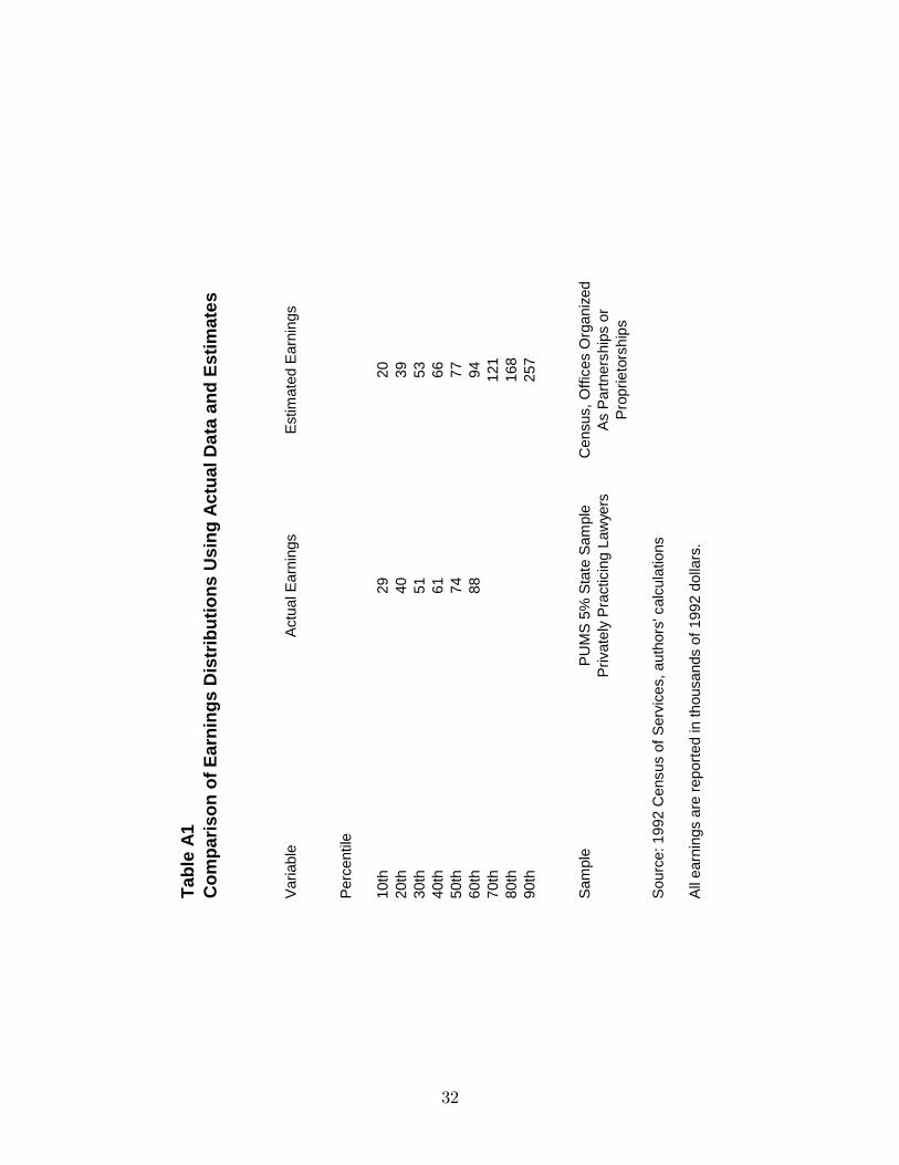
Tabl

e A1

Com

paris

on o

f Ear

ning

s D

istr

ibut

ions

 Usi

ng A

ctua

l Dat

a an

d Es

timat

es

Varia

ble

Actu

al E

arni

ngs

Estim

ated

 Ear

ning

s

Perc

entil

e

10th

2920

20th

4039

30th

5153

40th

6166

50th

7477

60th

8894

70th

121

80th

168

90th

257

Sam

ple

PUM

S 5%

 Sta

te S

ampl

eC

ensu

s, O

ffice

s O

rgan

ized

Priv

atel

y Pr

actic

ing 

Law

yers

As P

artn

ersh

ips 

orP

ropr

ieto

rshi

ps

Sour

ce: 1

992 

Cen

sus 

of S

ervi

ces,

 aut

hors

' cal

cula

tions

All e

arni

ngs 

are 

repo

rted 

in th

ousa

nds 

of 1

992 

dolla

rs.

32

…

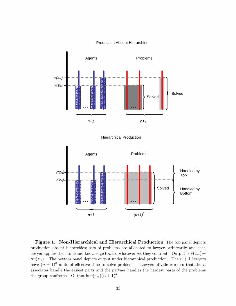
v(zm)_

…Solved

v(zw)

Production Absent Hierarchies

Agents Problems

n+1 n+1

Solved

…

v(zm)

…

Solved

Handled byTop

Handled byBottom

v(zw)

n+1 (n+1)θ

Hierarchical Production

Agents Problems

Figure 1. Non-Hierarchical and Hierarchical Production. The top panel depictsproduction absent hierarchies; sets of problems are allocated to lawyers arbitrarily and eachlawyer applies their time and knowledge toward whatever set they confront. Output is v(zm)+nv(zw). The bottom panel depicts output under hierarchical production. The n + 1 lawyershave (n + 1)� units of e¤ective time to solve problems. Lawyers divide work so that the nassociates handle the easiest parts and the partner handles the hardest parts of the problemsthe group confronts. Output is v(zm)(n+ 1)�.

33

40

6477

9410

711

712

613

815

416

718

019

521

2

235

260

296

341

410

531

4159

7991

9910

911

812

813

914

815

917

318

820

122

224

4

267

304

356

0100200300400500Thousands of 1992 Dollars

010

2030

4050

6070

8090

100

Perc

entil

e

Partn

er P

ayR(

0,th

eta)

Figure2.

TheDistribution

ofPartnerPay,Estimated

PartnerPay

AbsentHierarchies.ThisFigurereports20

quantilesofthedistributionofthesequantities,lookingonlyatpartnersato¢ceswithassociates."Estimatedpayabsenthierarchies�

isRi(z m

i;0).

34

320

3139

4753

6066

7277

8594

107

121

137

168

201

257

373

521

3139

4653

5966

7278

8593

103

116

131

151

180

222

284

0100200300400Thousands of 1992 Dollars

010

2030

4050

6070

8090

100

Perc

entil

e

Law

yer P

ayPa

y A

bsen

t Hie

rarc

hies

Figure3.

TheDistribution

ofLawyerPay,Estimated

PayAbsentHierarchies.ThisFigurereports20quantilesof

thedistributionofthesequantities.�Estimatedpayabsenthierarchies�isRi(z m;0)forpartnersato¢ceswithassociates.Itisthe

sameaslawyerpayforpartnersato¢ceswithoutassociates,aswellasforassociates.Becauseassociatesearnmoreasassociatesthan

theywouldabsenthierarchies(w(z)>Ri(z;0)),thisoverstateswhattheseindividualswouldearninthiscounterfactual.Thisupward

biasprimarilya¤ectsourestimatesoflowerquantiles.

35

2038 48 58 66 70 73 78 84 92 100

111122

135159

196

240

300

428

2139 49 58 66 70 74 79 87 92 99 108

120134

149

180

212

257

320

010

020

030

040

0 Lawy er Pay Pay  Absent Hierarchies

business, non­litigation off ices

­102 6 12 18 23 29 33 38 44 50 56 63 71

84101

119

156

208

­9 2 6 13 19 24 28 33 38 44 48 54 5970

8396

115

142

199

010

020

030

040

0Th

ousa

nds 

of 1

992 

Dol

lars

individual, non­litigation off ices

2337 43 50 55 60 65 71 77 85 92

105120

137161

182211

272

385

2437 44 50 55 60 65 72 77 83 91 101

114127

143160

185

222

286

010

020

030

040

0

0 10 20 30 40 50 60 70 80 90 100Percentile

litigation of f ices

Figure 4. The Distribution of Lawyer Pay, Estimated Pay Absent Hierar-chies, by O¢ ce Class. This Figure reports 20 quantiles of the distribution of these quantitiesfor three classes of o¢ ces. �Estimated pay absent hierarchies�is Ri(zm; 0) for partners at o¢ ceswith associates. It is the same as lawyer pay for partners at o¢ ces without associates, as well asfor associates. Because associates earn more as associates than they would absent hierarchies(w(z) > Ri(z; 0)), this overstates what these individuals would earn in this counterfactual.This upward bias primarily a¤ects our estimates of lower quantiles.

36