the role of 3d printing in biological anthropology · abstract the following work explores the role...
TRANSCRIPT

The Role of 3D Printing in Biological Anthropology
by
Travis T Allard
A Thesis submitted to the Faculty of Graduate Studies of
The University of Manitoba
in partial fulfilment of the requirements of the degree of
MASTER OF ARTS
Department of Anthropology
University of Manitoba
Winnipeg
Copyright © 2006 Travis T. Allard

Table of Contents Acknowledgements …..ii Abstract …..iii List of Tables …..iv List of Figures …..v Chapter I: Introduction …..1 Chapter II: Literature Review …..3 The Origin of 3D Printing …………………………… 4 Anatomical Modeling …………………………….…. 12 Rapid Prototyping in Anthropology ………………….15 Methods of Data Acquisition ………………………... 19 X-Ray Computed Tomography Scanning ……………. 20 3D Surface Scanning ………………………………… 29 Creating 3D Models from Virtual 3D Data ………….. 33 The Role of 3D Printing in Biological Anthropology ... 40 Chapter III: Virtual Reconstruction …..44 Objectives ……………………………………………... 45 Methods ……………………………………………..… 45 Results ……………………………………………….... 61 Discussion …………………………………………….. 67 Conclusion ……………………………………………. 69 Chapter IV: Skeletal Reproduction …..70 Objectives …………………………………………….. 70 Materials …………………………………………….... 71 Methods ……...……………………………………….. 72 Results ………………………………………………... 88 Discussion ……………………………………………. 101 Conclusion ……...……………………………………. 105 Chapter V: Discussion …..107 The Role of 3D Printing in Biological Anthropology .. 107 From Real to Virtual and Real Again ………………... 114 Chapter VI: Conclusion …..125 Work Cited …..128 Appendix I: List of Abbreviations …..133
i

Acknowledgements This work would not have been possible without the support and dedication of many people. First, I would like to acknowledge the generous support by Z-Corp in donating printing consumables. Other financial support throughout the course of this research was provided by the Canada Research Chairs program and the University of Manitoba. To Myra Sitchon, Dr. Roland Sawatzky and the Mennonite Heritage Village (Steinbach, Manitoba, Canada), I extend my sincerest gratitude for their insight and innovation in organizing the skeletal reproduction for the New Life exhibit. I would also like to thank Dr. Deborah Merrett, the University of Winnipeg, Dr. Martin Reed and the Dept. of Radiology, Sick Children’s Hospital for facilitating Case Study Two. Several figures in this thesis (2.1, 2.2, 2.3) illustrate aspects of CT data using the Bosma Collection (Shapiro and Richtsmeier 1997) which is now curated in the Dept. of Anthropology at the Pennsylvania State University. I also want to thank the members of my committee, Dr. Mary Silcox and Patrick Harrop, for their contribution to this work. Both challenged me to think more clearly and recognize my biases. They have contributed immensely not only to this work but to my overall intellectual development as well. Thank you. A very special recognition goes out to my advisor Dr. Robert D. Hoppa. Most of his student’s know him as Rob, and he is the most inspiring mentor anyone could be blessed to work with. Rob has challenged me and given me great freedom to achieve far beyond what I could ever dream possible. It is Rob I thank for this passage into the next phase of my life with more strength and wisdom than I have ever had. My greatest gratitude to the best advisor ever, Dr. Robert D. Hoppa. In every major achievement there are always struggles. The people that surround us have an impact on how such things work out. For this, I would like to thank Dr. Dave Stymeist and Dr. Greg Monks. I also want to thank Enza Pohl, Dr. Heather Gill-Robinson and Barb Hewitt for their support and insight. All of you add or have added greatly to the richness of character and vibrancy of the department and my experience there. Lastly, I want to dedicate this work to my wife, Lyndsey Smith, for her strength, stability and patience throughout this time. The past three years have been a time of tremendous growth for both of us, and I am glad we could share in this together. Without you Lyndsey, this truly would have never been possible. I also dedicate this work to my family that has been there through thick and thin and even pulled me out of the thick from time to time. Thank you to Grandma “G”, Dad and Joyce. A special thanks to Dad and Joyce for teaching me to follow through with what I started, and honour the commitments I make.
ii

Abstract
The following work explores the role of 3D printing in biological anthropology. A case study approach is used to provide an understanding of two different applications for 3D printing and to identify a potential methodology for creating 3D models. Case study one looks at the application of 3D printing to reconstruction projects using a flowerpot to test the reconstruction methodology. The second case study uses both laser surface and CT scanning to create a replica of a human skeleton. The two methods of data acquisition are evaluated for advantages and limitations in creating the virtual model. This work shows that there is a role for 3D printing in biological anthropology, but that data acquisition and processing issues are the most significant limiting factors in producing skeletal replicas.
iii

List of Tables Chapter III: Table 3.1: Original and Printed Pot Comparison …………………………..….. 61 Table 3.2: Unbroken and Reconstructed Differences ………………….……… 64 Chapter IV: Table 4.1: Surface Scan Summary …………………………………………….. 74 Table 4.2: Total Deviation Between Surface and CT Scan Data ……………… 89 Table 4.3: Skull and Sacrum Comparison of Virtual and Printed Models …….. 98 Chapter V: Table 5.1: Numerical Results of Acquisition Method Comparison ……………. 116
iv

List of Figures Chapter II: Figure 2.1: Partial Volume Effect ……………………………………………24 Figure 2.2: Beam Hardening …………………………………………………25 Figure 2.3: Frozen Noise ………………………………………………….….26 Figure 2.4: Non-Manifold Face …………………………………………...….37 Figure 2.5: Runaway Feature …………………………………………….…..38 Figure 2.6: Z-406 Build Chamber ……………………………………………42 Chapter III: Figure 3.1: Original Flowerpot ………………………………………………46 Figure 3.2 Scanning Diagram ………………………………………………..47 Figure 3.3: Camera and Laser Angle for Optimum Scanning …………….…48 Figure 3.4: Final Virtual Model of Unbroken Flowerpot …………………....50 Figure 3.5: Unbroken Flowerpot Post-processing Method Two …………….51 Figure 3.6: Broken Flowerpot ……………………………………………….51 Figure 3.7: Shard Models …………………………………………………....52 Figure 3.8: Thin Shard to Thick Shard ……………………………………....53 Figure 3.9: Reconstruction Using Volume Shards …………………………..54 Figure 3.10: Thin-wall Registration ………………………………………....55 Figure 3.11: After Hole Filling and Smoothing ……………………………..56 Figure 3.12: Final Virtual Model Using Reconstruction Method Two ……...57 Figure 3.13: Virtual Models of Unbroken and Reconstructed Flowerpots ….58 Figure 3.14: Unbroken Model Using Post-Processing Method One ………...59 Figure 3.15: Unbroken Model Using Post-Processing Method Two ………..59 Figure 3.16: Reconstructed Model Using Method Two ……………………..60 Figure 3.17: Reconstructed Model Three (Combined Methods) …………….60 Figure 3.18: Side View of Flowerpot Inspection Results ……………………65 Figure 3.19: Top/Inside View of Flowerpot Inspection Results ……………..66 Figure 3.20: Colour Model of Flowerpot Differences ……………………….68 Chapter IV: Figure 4.1: General Scanning for Bones …………………………………….72 Figure 4.2: Registration Process Step One …………………………………..76 Figure 4.3: Result of Registration ……………………………………………77 Figure 4.4: Simplification ……………………………………………………78 Figure 4.5: Model Detailing ………………………………………………….79 Figure 4.6: Series One ………………………………………………………..80 Figure 4.7: Series Two ……………………………………………………….81 Figure 4.8: Series Three ……………………………………………………...81 Figure 4.9: Series Four ……………………………………………………….82 Figure 4.10: Series Five ………………………………………………………82
v

List of Figures Continued Figure 4.11: CT Position Error …………………………………………….83 Figure 4.12: Working in Mimics …………………………………………..84 Figure 4.13: Segmented Elements …………………………………………85 Figure 4.14: Joining the Proximal and Distal Femurs ……………………..87 Figure 4.15: Completed Long Bone ……………………………………….88 Figure 4.16: CT vs. Surface Scan for Left Clavicle ……………………….90 Figure 4.17: Registered CT and Surface Scans of the Skull ……………….91 Figure 4.18: Innominate Inspection ………………………………………..92 Figure 4.19: Left Humerus Inspection ……………………………………..93 Figure 4.20: Left Scapula Inspection ………………………………………93 Figure 4.21: Right Clavicle Inspection …………………………………….94 Figure 4.22: Right Humerus Inspection ……………………………………95 Figure 4.23: Left Ulna Inspection ………………………………………….96 Figure 4.24: Right Ulna Inspection ………………………………………...96 Figure 4.25: Skull Inspection ………………………………………………97 Figure 4.26: New Life Exhibit ……………………………………………..99 Figure 4.27: Skeletal Reproduction ………………………………………..100 Figure 4.28: CT and Surface Scan Comparison Models …………………..104 Chapter V: Figure 5.1: Seamless Long Bones …………………………………………113 Figure 5.2: Visual-Spatial Data Analysis Using 3D Object ……………….117 Figure 5.3: Colour Bone Density Model of Mandible ……………………..121
vi

Chapter I: Introduction
________________________________________________________________________
The goal of this work is to investigate the role of 3D printing in biological
anthropology. 3D printing is a method of producing physical models using computer-
generated data. Weber (2001) discusses the increasing use of technology in anthropology
and how, despite the conservative nature of anthropological research, new technologies
are going to change the way in which we approach research in the future. 3D printing is
one of those technologies waiting for regular use in biological anthropology. Before this
more widespread use occurs, researchers need to understand how 3D printing can be used
and exactly what it is. This work is intended to provide a basic understanding of how to
use 3D printing in biological anthropology. This basic introduction to the advantages and
limitations is necessary for a conceptual appreciation of the role of 3D printing for future
projects.
Chapter II provides an introduction to the wider topic of rapid prototyping as it
applies to the birth of 3D printing technology. This discussion describes the rationale for
choosing the 3D printing approach to rapid prototyping over other approaches. An
overview of anatomical modeling and the use of rapid prototyping in anthropology to
date provides context for the later discussion of the role of 3D printing. The final section
of this chapter outlines the objectives of the following work and the case studies used to
explore the role of 3D printing in biological anthropology. Two case studies form the
basis for this discussion and also provide a methodological guideline for future research.
Chapter III presents the first case study. Case study one is a look at the use of 3D
printing for reconstruction projects in biological anthropology. A flowerpot is used as a
1

pilot for exploring a reconstruction method that involves 3D printing. The reconstruction
efforts were not entirely successful. More research is needed into better reconstruction
methods prior to using skeletal material. This case study does outline the use of 3D laser
scanning and some principals for using 3D printing in reconstruction projects.
Chapter IV presents case study two, the creation of a skeletal replica using both
3D laser scanning and computed tomography scanning as data acquisition methods. This
case study builds on some of the lessons learned in the previous case study and evaluates
the differences between the two acquisition methods (laser surface scanning and
computed tomography scanning). This case study also describes the use of the skeletal
replica in a museum exhibit.
Chapter V explores the role of 3D printing in anthropology from a more
conceptual viewpoint. The case studies are intended to give a methodological
understanding of the ways in which 3D printing can be used and this chapter explores
what the results mean to researchers in biological anthropology. In particular McLuhan’s
(1966) notion of the “medium is the message” is explored as it relates to 3D printing in
biological anthropology.
Chapter VI concludes the discussion on the role of 3D printing in biological
anthropology. This chapter summarizes the results of the exploration of methodology
and the potential future role of 3D printing in biological anthropology. Future directions
for this research are presented.
2

Chapter II: Literature Review
______________________________________________________________________
The term rapid prototyping (RP) refers to a process of manufacturing computer-
generated models by adding consecutive layers of material to build a physical 3D object.
There are many different adaptations of this approach that have resulted in a variety of
devices each with their own unique features and types of building materials. In order to
address the role of rapid prototyping in biological anthropology, it is important to
understand the origins and impetus for the development of this technology.
Understanding this history will facilitate a better grasp of the future directions and
limitations for this technology in anthropology.
It is also necessary to review how data is gathered and used for the RP process in
biological anthropology. Originally RP was developed for the manufacturing industry
utilizing computer assisted design (CAD) data for the RP process. The CAD data
represent the authors’ computer-generated design concept and is validated using the
physical object from the RP process. In contrast to this, studies in biological
anthropology using RP first require making a digital replica of an item that already
physically exists, such as a skull, and then reproducing it using the RP technology.. This
process is known in the industrial world as reverse engineering. There are several
different ways data can be acquired to produce the output for the RP process following a
reverse engineering approach. Two of the most common methods for studies in
biological anthropology are laser surface scanning and X-ray computed tomography (CT)
scanning. A discussion of the types of data derived from these two processes is essential
for understanding the role and limitations of RP in biological anthropology.
3

The Origin of 3D Printing
Rapid Prototyping (RP) is a generic term that was introduced with the release of
the first device in the 1980s (Grimm 2004). This use of the term RP is linked to the
marketing of the technology to the engineering and product-design industries. RP was
intended to replace computer numerical control (CNC) manufacturing, a process that
subtracts material from a larger block to yield a physical object from CAD data. CNC
manufacturing was developed out of the merger between traditional lathing and computer
programming and was the first computer automated manufacturing process.
CNC devices use a cutting tool controlled by a user-guided computer algorithm to
carve the desired shape out of a larger block of material. Since CNC devices cut away
material from a larger base, they are limited to producing models of external features. RP
devices were introduced to overcome this barrier and are capable of producing internal
structures as well, such as the internal sinuses in a skull. CNC manufacturing also has
difficulty producing very complicated external features, especially deep holes and slots
(Grimm and Wohlers 2003). The interface between the user and the device is also more
complicated for CNC manufacturing, often requiring specialized training for the operator
(Grimm 2004, Grimm and Wohlers 2003, Seely 2004). The proliferation of RP devices
particularly in the educational environment is partially attributed to the ease of use of the
technology over CNC manufacturing (Seely 2004). Grimm (2004) does note that both
CNC and RP devices produce models relatively quickly. However, RP does not require
extensive training to operate, meaning the overall process of design to model is faster
than with CNC manufacturing (Grimm 2004).
4

CNC manufacturing still has a number of advantages over the more recent RP
technology. RP devices are limited to a range in build chamber sizes (203 mm3 to
610mm X 914mm X 508mm), where as CNC manufacturing is capable of handling items
as large as aerospace parts (Grimm 2004). CNC is also more accurate, with results
ranging from 0.03mm to 0.13mm, whereas RP is accurate to between 0.13mm and
0.76mm (Grimm 2004). Finally, RP devices are also limited in the range of materials
that can be used and CNC devices are capable of accepting virtually any material (Grimm
2004, Grimm and Wohlers 2003). Both RP and CNC have advantages and
disadvantages. The decision to use one or the other is related to the project (Grimm
2004, Grimm and Wohlers 2003).
CNC manufacturing was successfully used to produce the moulds for the creation
of the tiles used to make the replica of the tomb of Seti I (Ahmon 2004). The CNC
device used in this case was able to handle the manufacturing of the large blocks; the
researchers were also reproducing only the visible surface that was ornate but not
topographically complicated. There is currently no RP technology capable of producing
models as large as the blocks used for the creation of the tomb. In the case of the
recreation of the tomb of Seti I, CNC manufacturing was the most appropriate technology
to use. For applications in biological anthropology RP is likely the best approach.
Unlike the engineering and manufacturing disciplines, it is important to have a device
that can be used with minimal investment in training. The size constraints are less of an
issue in biological anthropology as well, where the focus is primarily on human bones.
Most importantly, the ability to reproduce internal structures and complicated surfaces is
5

important to creating skeletal replicas. Skeletal elements are often morphologically
complicated and have many canals and similar structures that are best produced using RP.
On March 11th, 1986, Charles Hull received patent number 4575330 “Apparatus
for Production of Three-Dimensional Objects by Stereolithography” (Grimm 2004: 15).
This patent was the beginning of the RP approach to physical model creation from CAD
data. The construction of a 3D model from 2D layers successively organized on the Z-
axis allows for the creation of both internal and external surfaces. In 1988, 3D Systems
Incorporated released the first commercial stereolithography (SLA) device based on
Hull’s patent and termed the process “rapid prototyping”. Since this first SLA device, a
number of different technologies have been released based on a similar approach. These
technologies are typically all grouped under the RP heading, although the term originated
with SLA. The resulting technological approaches have spread to a variety of industries
and most recently, academic research.
RP has now become a confusing blanket term to generically describe many
different technologies, all of which are based on the same computer to model, additive-
based approach to 3D object creation. Zollikofer and Ponce de Leon (2005: 209) discuss
the term “real virtuality” as being synonymous with RP. In this instance, the focus is on
the model as a facsimile of reality, thus they link 3D object creation to a method of
making virtual reality tangible. Another term used to describe RP is 3D Printing (3DP).
3DP is sometimes used to refer to all RP technologies, and sometimes to specific
approaches to RP (Grimm 2004). However, both rapid prototyping and 3D printing carry
a specific meaning tied to its particular usage. As suggested by Grimm (2004), RP will
be used in this work to describe the total range of additive-based production methods
6

from computer generated 3D models. This will ensure continuity with other available
literature and help to establish consistency in terms. 3DP will refer to a specific
technology marketed by Z-Corp, which falls under the RP umbrella. Real virtuality will
be addressed during the discussion of the role of 3D printing in relation to the crossover
of this technology from industry to academe in Chapter V.
The varieties of RP technologies are based on one of five key methods: curing,
sheeting, dispensing, sintering or binding (Upcraft and Fletcher 2003). Curing involves
solidifying photosensitive resins using a focused light source such as a laser. The SLA
technology patented by Hull uses this approach. The only materials available for SLA
are epoxy-based resins (Upcraft and Fletcher 2003). Having only one available material
limits the range of possibilities in part quality and versatility. Sheeting, or Laminated
Object Manufacturing (LOM) relies on the application of consecutive layers of material
that are cut to shape as they are layered on the z-axis. The materials available are paper,
polyester/polyethylene, ceramic coated paper and polycarbonate composites (Upcraft and
Fletcher 2003). Dispensing utilizes a systematic discharge of a filament onto a specified
area, the part is grown from the result of successive deposits. This process is also known
as Fused Deposition Modeling (FDM). The materials available for this include
thermoplastic (acrylonitrile butadiene styrene, or ABS), elastomer, wax and
polycarbonate (Upcraft and Fletcher 2003). Sintering (Selective Laser Sintering) is
similar to SLA, except that heat sensitive powders are solidified using a concentrated heat
source, instead of photosensitive resins. Several different materials are available for this
process such as carbon steel, nylon, polystyrene, polycarbonate, wax, ceramics,
zirconium sand and flexible elastomere (Upcraft and Fletcher 2003). Binding (the
7

binder-jet process) also uses powders but with a gluing solution rather than a heat source
to solidify the powder into the desired shape. This process uses either starch or plaster
(Upcraft and Fletcher 2003: 326). The binder-jet process is often referred to as 3D
Printing (3DP) because it uses print-head technology similar to a bubble-jet printer
(Grimm 2004).
Each of the above-mentioned approaches has both strengths and weaknesses.
Users choose a technique based on the desired printing medium, and part properties such
as accuracy, durability, and production cost. In an effort to give new and prospective
users a more objective overview of what to expect from RP systems than what is
available from manufacturers, Grimm (2004) tested four of the leading machines. In this
overview, the Viper si2 SLA, Vangaurd si2 SLS, Titan FDM and Z-406 3DP were
assessed for part accuracy, stability, feature definition and speed. Grimm qualifies these
results by stating that they cannot be analyzed statistically since they are based on a
single trial of one part on just four machines. Neither inter-observer nor intra-observer
error is reported for these tests since they are based on only one trial. The results
however, do give potential users a base-line of what to expect from each method.
Grimm’s assessment of accuracy is measured through average material shrinkage
over a series of measurements. SLA and FDM are the best and 3DP the worst (Grimm
2004). Grimm reports average total deviation for each system as follows: SLA 0.8
percent, SLS 1.2 percent, FDM 0.5 percent and 3DP 1.4 percent. In contrast to the parts
built using the other technologies, the 3DP part is built in a chamber of loose powder.
The powder is used to support and suspend the object during the printing process.
Unfortunately, the action of natural forces such as gravity can have a negative impact on
8

parts built using 3DP. Lee and colleagues (1995) suggest that layer displacement from the
compaction of powder in the build chamber, may contribute to part inaccuracy for the
3DP process. The centre of the build chamber is the most volatile for both compression
and layer displacement (Lee et al. 1995). Therefore parts built in the center of the
chamber may be subjected to additional compression affecting overall accuracy.
Part accuracy is relative to the overall purpose of the part being printed. While
SLA is more accurate than 3DP by a factor of 0.6 percent, it may not be as cost effective
or as quick. For concept modeling (demonstrating product design ideas) this is an
acceptable trade-off. The purpose of the final object is to convey a physical
representation of a design idea that does not need to be highly accurate. In this case
speed and cost efficiency are more beneficial traits. In applications involving a reverse
engineering approach (such as with studies in biological anthropology), it is important to
match the spatial resolution of the data acquisition device with the approach with the
most appropriate accuracy potential. For example, the 1.4 percent difference in the
original part and the part printed using the 3DP method corresponds to a difference in
linear dimensions of –0.38mm for shrinkage and 0.64 mm for expansion. Some data sets
are based on CT scans, and can range in spatial resolution from 2mm slices to 0.04mm
slices. A user’s understanding of the capabilities of a rapid prototyping method should be
framed in the context of the application and data source being replicated.
Part stability, as measured by Grimm (2004) refers to the degree of change in
size and shape of parts over time. This assessment is more closely related to the
properties of the production mediums than the actual machine capabilities. Part stability
can improve with advancements in consumable materials used by each technology.
9

Grimm reports that SLA is not stable over time and that a limitation of the photosensitive
resins is their susceptibility to distortion from heat, moisture and chemical agents. Both
SLS and FDM materials are stable when removed from the build chamber. 3DP parts are
not stable when removed from the build chamber, but can be made stable through post-
processing infiltration with wax, epoxy or cyanoacrylate (CA). When this is done the
parts take on the material properties of the infiltration medium. This is because the bonds
between plaster particles are far enough apart to allow for the infiltration medium to
envelop the entire structure, encapsulating the bonded starch or plaster particles (personal
communication, Z-Corp).
Feature definition refers to the smallest amount of detail that can be produced by
each method. Grimm (2004) notes that the theoretical feature size capable of being built
using any given approach is not necessarily equivalent to what will survive removal from
the build chamber. The tested values Grimm reports are realistic to what the user can
expect after removing the part from the build chamber. The minimum feature size for
each system is as follows: SLA 0.51mm, SLS 0.64mm, FDM 0.41 to 0.61mm and 3DP
0.76 to 1.52mm. Grimm does not report these values in terms of 3D structures leading
the reader to assume that the values presented correspond to the smallest feature cubed.
These results relate to the material properties of the printing medium and the user’s skill
at retrieving items from the build chamber. Parts printed using the 3DP process are
usually weakest in the initial few hours following print completion. This is known as
“green strength” and is the most limiting factor of the 3DP method. Small features have a
tendency to break when being excavated from the powder in the build chamber; this is a
significant limitation of the 3DP technology. Recent advances in the Z-510 (Z-Corp’s
10

replacement for the Z-406 in 2005), such as a heated build chamber and stronger material
systems should change the minimum feature size capable of being produced with the 3DP
technology. Similar to the discussion on accuracy, feature size limitations should also be
considered with the resolution of the original data in mind. The printer will not be able to
print features smaller than the resolution of the source data.
The SLA technology performs well on both the accuracy and feature definition
categories of Grimm’s assessment, while the 3DP technology comes up short next to
SLA. Production speed is where the 3DP technology wins out over the other methods
(SLA, SLS and FDM). The SLA technology performed the worst. The methods
evaluated in Grimm’s previous tests yielded the following time results for the same part
(measuring 15.24 x10.16 x 1.91 cm): SLA 5.4 hours, SLS 1.5 hours, FDM 4.2 hours and
3DP 35 minutes. Faster machines for the SLA and FDM methods were also tested and
included in Grimm’s report on speed, but were not included in the other tests for accuracy
and feature definition. It is therefore difficult to include the faster models in a fair
comparison between the different methods.
Since the mid to late 1990’s the number of different approaches to RP have
increased the availability of this technology and allowed for the development of a range
of technological options for consumers. An often-asked question is how RP can be used
in specific industries (Carrion 1997, Grimm 2004, Kochan 2000). RP technologies are
primarily used to communicate information about concept designs, analytical results and
related visual and tactile information. Grimm (2004: 35) writes, “since rapid prototyping
requires no manipulation or human interpretation of the design data, its direct output
offers design verification”. Discussing attributes about an object is potentially more
11

effective than discussing either a written description or photograph. Holding the physical
object in question allows the interpreter to freely associate with the object, without
complicating issues such as industry-specific discourse in a written account or
photographic bias. Consider the difference between learning osteology from a textbook
only versus actually holding the bones. The student gains a richer appreciation for
subject material by handling the actual bones than simply reading about them or looking
at pictures. The same is true for communicating design ideas to an audience of potential
clients (especially when the clients are not from a design related field). The
interpretation of the object is not filtered through someone else, as is the case with written
descriptions or photographs, which represent the object as the writer or photographer
viewed it. The most obvious use of RP is therefore in communicating complex design,
shape or form concepts. In support of this, Zollikofer (2005) cautions that RP is not an
analytical tool, but simply a tool used to share information.
Anatomical Modeling
RP technology was originally developed for the design and manufacturing
industries. Recently, biomedical applications for RP have flourished beyond what was
originally imagined for the technology. The majority of this usage is reported in case
studies where RP has been used in novel ways to solve biomedical problems. Zollikofer
and Ponce de Leon (2005) note that RP enhances surgical planning, custom implant
design, case collection and teaching. The key breakthrough is the ability to non-
invasively reproduce physical 3D models from 3D medical scan data of living or dead
subjects. The advantages of using 3D models in a surgical context include more effective
and accurate pre-operative planning and better surgeon to patient communication.
12

Powers (1998) reports that the use of 3D models in surgical planning reduces both the
length of surgeries and the chance of mortality. Many of these studies have focused on
using SLA technology and most examples focus on surgical applications (e.g. Anderl et
al., 1994; Borah et al., 2001; Brown et al., 2001 & 2003; Hieu et al. 2005; Perez-Arjona
et al., 2003).
The linear accuracy of SLA models is also well established in the biomedical
literature (Barker et al., 1994; Bouyssie et al., 1997; Choi et al., 2002; Ono et al., 2000,
Wulf et al. 2001). Barker and colleagues (1994) and Choi and colleagues (2002) examine
the accuracy of SLA models by comparing deviation in linear measurements between dry
skulls and their model analogues. Both studies utilized CT data for the creation of the
virtual 3D models. Choi and colleagues also considered the accuracy of the CT data used
to create the SLA model. They raise the important point that the model is only as good as
the original data. Their CT scan was performed with 1mm slices, making maximum
resolution limited by this margin of error. Choi and colleagues (2002) report the
accuracy of their skull models over 16 landmark-based measurements to be within
0.62mm, +/- 0.35mm. They note that this is smaller than previously reported values by
other researchers. The earlier study by Barker and colleagues reports an overall average
difference of 0.85mm between the skulls and skull models. This is based on a
comparison of four linear measurements of 11 skulls over five trials. Bouyssie and
colleagues (1997) published a similar study investigating accuracy of SLA models from
CT data using only mandibles instead of complete skulls. They state that there is no
statistically significant difference between the original and the SLA replicas of 12
mandibles. Bouyssie and colleagues report an average difference in measurements
13

between the models and original mandibles as 0.12mm. This value was compared to the
standard error of the mean (0.02mm) using a Student’s t-test with an ∝ level of 0.005.
According to this analysis, they conclude that there is no statistically significant
difference between the original and model. The ability of SLA to reproduce almost
exact RP replicas of original objects is fairly well documented by the literature to date.
Accuracy-based assessments in the anatomical modeling literature consistently note that
significant sources of error result from either observational biases, such as landmark
replication, or data acquisition error (Barker et al., 1994; Bouyssie et al., 1997; Choi et
al., 2002; Clark et al. 2004; D’Urso et al. 2000; Hjalgrim et al. 1995; Ono et al., 2000).
The real test of RP technology is how it can be used to solve particular communication
and visualization problems. Borah and colleagues (2001) find that models provide an
independent evaluation of biological architecture through a material of known uniform
properties. They use 3D models to represent microscopic structures such as trabecular
bone. The model is then subjected to stress tests, which assess the geometric tolerance of
the structure alone without the added complication of multiple substances and varying
chemical composition. Borah and colleagues have been able to understand changes in
bone strength relative to bone loss in patients suffering from osteoporosis using 3D
models of real bones. Bibb and Sisias (2002) performed a similar study aimed at
validating finite element analysis (FEA) results from µCT data of cancellous bone.
Another important application explored for SLA replicas is the ability to
reproduce specific regions of interest for surgeons and allow more effective pre-operative
planning (Hieu et al. 2005). Brown and colleagues (2003) examined this by looking at
117 patients with complicated fractures and using SLA models of those fractures to
14

improve surgical success rate. One such successful example they site is the use of the
SLA models for planning the trajectory of screws used in the treatment of a spinal injury.
Brown and colleagues (2001) reported similar success for the treatment of a hip fracture.
Anderl and colleagues (1994) used SLA for planning a sensitive osteotomy (surgical
removal of bone tissue) on an eight-month-old patient requiring extensive reconstructive
craniofacial surgery. In these cases, SLA models allow surgeons to visualize tangible
replicas of the patient’s bodies and plan “what-if” scenarios, without having to make
contact with the patient. Related to surgical applications are the medical-legal
implications for RP technology in general. Dolz and colleagues (2000) present a case
study in which an SLA model of a child’s skull was presented during a child abuse trial.
They argue that presenting the model of the fracture patterns is less inflammatory and
more dignifying to the victim than presenting photographs.
Rapid Prototyping in Anthropology
While the biomedical community is making use of RP, less work has been done in
anthropology to assess the usefulness of this technology. The most important possible
advantage to using RP in anthropology is the ability to non-destructively create models of
the past for further study. Hjalgrim and colleagues (1995) used CT scans to non-
invasively create a 3D model of an ancient Egyptian mummy skull. This approach
allowed the researchers to examine the skeletal structure of the individual without having
to physically manipulate or unwrap the mummy. Ancient remains in particular are
precious resources, and can often be associated with a need for cultural sensitivity.
Hjalgrim and colleagues (1995) further noted that it was possible to perform traditional
methods of anthropological analysis (such as sexing and estimating ancestry) on the
15

model without having to disturb the original specimen. D’Urso and colleagues (2000)
contrast traditional approaches to anatomical modeling such as using casts with RP.
Creating casts of specimens requires making contact and adhering molding compounds to
the original item’s surface. This approach has the potential to damage the surface of the
object, and makes it difficult to capture detail such as internal cranial structures (D’Urso
et al. 2000).
In anthropology, one of the first reports of 3D modeling is from the investigation
of the Tyrolean Iceman found in the Alps (Weber, 2001b; zur Nedden, 1994). Every
effort to preserve the original condition of this mummy was taken; therefore conservation
focused on replicating the preservation environment. This meant that the iceman could
not leave the freezer long enough to be studied. A full CT scan was performed in order
to provide researchers with images of the skeleton and other associated artefacts. An
SLA model of the Iceman’s skull was made for further analysis and facial reconstruction.
This proved to be a breakthrough in the limitations of working with limited and precious
resources. The model of the Iceman’s head could be shown and handled by researchers
without disturbing the very delicate nature of the mummified individual. The SLA model
effectively replicated the structural and anatomical anomalies such as the flattening of the
face, which was not as clearly visible in the CT scans (zur Nedden et al. 1994). In this
case, SLA was also used to create models to inform the public while the body was kept
safely curated.
Zollikofer and Ponce de Leon (2005) outline that RP can be used in
paleoanthropology for direct replication, replication of hidden structures (as in fossils
encased in matrix), and for validating and reproducing virtual reconstructions. D’Urso
16

and colleagues (2000) and Clark et al. (2004) each used SLA to create replicas of a fossil
still encased in matrix. Although both of these studies examine non-primate
paleontological material, the same principals apply to using the imaging and RP methods
on fossils of anthropological significance. When there is sufficient difference between the
fossil and matrix, the outline of the fossil can be distinguished from the matrix by shape
and density differences as observed in a CT scan. The fossil or object can then be
segmented out and reproduced without the need to attempt further excavation. This is
important because excavating fossils from dense matrix can be dangerous to the precious
resources. The models can then be made permanently available, and internal structures
never before seen can be reproduced and examined (Weber 2001). All of these examples
of RP focus on using SLA technology.
While there are many different RP technologies available, researchers do not
report why SLA was chosen over other approaches. SLA is one of the first and most
broadly available RP technologies. In addition to this, some researchers note a
knowledge, or communication gap between biomedical and engineering communities
(Fontana et al. 2002, Hieu et al. 2005). A lack of awareness of the variety of RP methods
available by biomedical and anthropological researchers may contribute to the bias
towards using SLA technology. The novelty of the relatively recent uses of SLA may
also over-shadow a more critical examination of the usefulness of the different RP
approaches for specific projects.
Another significant barrier to the use of RP and in particular SLA is cost (Dolz et
al. 2000, Hieu et al. 2005, Hjalgrim et al. 1995, Powers 1998). Dolz and colleagues
(2000) give general figures for cost and speed of the SLA models for their purposes.
17

They estimate that a single case may range from $2000 to $3000 and if rushed will be
ready within two to three days. Hjalgrim and colleagues (1995) go a step further and
report the SLA model of an Egyptian skull they produced resulted in a total consumables
cost of $2500 (US) and took 40 hours to build. The photosensitive resin is a very
expensive material. The high cost of SLA consumables is a widely accepted and
recognized drawback for the technology (Grimm 2004). The lack of widespread use of
RP in research environments is likely due to the combination of SLA being both the most
broadly available and the most expensive approach. Researchers will naturally tend to
use RP for exceptional projects such as the reproduction of the skull of the Iceman by
Hjalgrim and colleagues (1995). A more cost-friendly approach to RP may increase not
only the use of RP in research environments, but also the overall availability and breadth
of projects in which it can be used.
Ono and colleagues (2000) report that the 3DP method of printing models is able
to overcome the cost barrier, which has prevented the use of RP in everyday research. In
their study, Ono and colleagues (2000) compare the accuracy and viability of skulls
printed using the binder-jet method and the standard SLA method. They find that the
binder-jet method is not only more cost effective, but is also capable of producing better
anatomical specimens. The plaster-based materials of the 3DP method are capable of
reproducing complex structures without the support struts often needed for SLA models
of the skull in orbits, sinuses and the cavities at the base of the skull (Ono et al. 2000:
532). As well, the binder-jet method is capable of reproducing finer surface detail such
as pores and nerve cavities (Ono et al. 2000: 532). Irregularities in surface morphology
18

are important to anatomical modeling, especially for disciplines such as biological
anthropology that focus on examining variation in biological form.
The transparency of the semi-translucent SLA material is an advantage for seeing
structures under the surface morphology. While losing this benefit, the binder-jet method
is capable of adding colour to objects. Gibson and Ming (2001) note that colour has been
traditionally limited to the manufacturing and architectural industries to distinguish
regions of parts, design iterations or artistic flare. In contrast to this, few researchers
have experimented with the use of colour in anatomical modeling. The 3D printers
marketed by Z-Corp offer potential to enhance anatomical modeling through the use of
colour 3DP. Colour is also available in a limited fashion by LOM (Gibson and Ming
2001).
To date, there are few examples of anatomical modeling using 3DP technology.
This is likely due to the point that the first 3DP platforms were only released in 1999
(Grimm 2004). The 3DP technology needs to be examined further to better understand
its potential role in anatomical modeling.
Methods of Data Acquisition
The RP process is dependant upon a virtual model created using a variety of
methods such as CAD, CT scanning or surface laser scanning to name a few. The
following section will provide an overview of data acquisition as it applies to anatomical
modeling in anthropology. The focus will be on the limitations and possibilities of using
CT and surface scanning in biological anthropology. The final section of this review of
data acquisition will examine some basic issues associated with the creation of virtual 3D
models.
19

The literature discussed in this chapter cites the process of data acquisition as the
most significant limiting factor for spatial resolution and accuracy of RP models (Barker
et al.., 1994; Bouyssie et al., 1997; Choi et al., 2002; Clark et al. 2004; D’Urso et al.
2000; Hjalgrim et al. 1995; Ono et al., 2000). These researchers utilized CT data for the
creation of models. The following section will briefly examine some of the fundamental
bases of CT scanning, and the emerging use of 3D laser scanning to produce both
physical and virtual surface models and end with a brief discussion on file formats
including some of the errors that can occur in the printing process from poorly prepared
files.
X-Ray Computed Tomography Scanning
X-ray CT scanning has become a common and accepted method of data
acquisition in biological anthropology (Spoor et al. 2000, Weber 2001a and 2001b,
Zollikofer and Ponce de Leon 2005). While RP is still a relatively novel application in
anthropology, the use of CT as a viable method of data acquisition has been well
explored for non-invasive visualization in palaeoanthropology, palaeopathology and
morphometric studies. Mehta (1997) concludes that CT scanning is an effective method
of acquiring data allowing one to visualize 3D reconstructions of bone. This makes CT
scanning ideal for most anthropological applications, where dose is not as great a concern
for skeletal remains versus living patients for biomedicine. Lynnerup and colleagues
(1997) highlight the non-invasive aspects of CT scanning archaeological material, one of
the principal advantages of using this type of data acquisition. Wood (2000) also notes
that CT scanning helps identify fossilized bone from matrix, avoiding potentially
damaging cleaning methods. Perez and colleagues (2000) illustrate that the 3D structure
20

of hidden anatomy such as nasal cavities can be effectively studied using CT scanning.
Ruhli and colleagues (2002a,b) show how CT scanning significantly enhanced diagnosis
of palaeopathological lesions by more effectively visualizing structures. In particular,
Ruhli and colleagues ( 2002a) demonstrate that the multi-detector CT approach used
increased spatial resolution for more effective diagnosis of cranial lesions for three
ancient cases. Multi-detector CT scanning utilizes several collection devices to
simultaneously record multiple angles of the subject being scanned. Pasquier and
colleagues (1999) use CT scans to create a more effective numerical scoring for age-at-
death estimation using the Suchey-Brooks casts. The correlation coefficient they report
for the comparison between virtually identified pubic symphyses and those identified
from direct observation is 0.74. This result does show a relationship, but it is weak in the
context of providing meaningful conclusions about age at death. Evolutionary analysis
and morphometric studies also commonly use data obtained through CT scanning (eg.,
Brown and Wood 1999; Williams and Richtsmeier 2003, Zumpano and Richtsmeier 2003
to name a few such studies). The purpose of this section is not to explore CT scanning in
biological anthropology per se, but to show that this method is well established as a
valuable tool in anthropological studies and introduce the advantages and limitations.
These advantages and limitations have a bearing on the use of CT scanning with RP
applications. RP can be used to extend the advantages of non-invasive study to tangible
and accurate replicas of scanned specimens.
The general process for using CT data requires 3 basic steps. The first is
recording the object using a CT scanner. From the CT scanner, files are typically
exported as raw or DICOM (Digital Imaging and Communications in Medicine) formats.
21

Both file formats are composed of a series of 2D images each representing a section of
the imaged object. The images must then be imported and visualized using an imaging
program where structures can be isolated as regions of interest and 3D rendering can take
place if required. The potential for data problems exist at each stage of the CT process
illustrated above. Understanding CT data acquisition and processing is integral to the
effective use of this data in anatomical modeling and biological studies (Zollikofer and
Ponce de Leon 2005). Lester and Olds (2001) emphasize that it is important to consider
the nature of the data required before attempting any imaging study.
Like traditional radiography, CT uses the passage of X-rays through an object and
records the resulting attenuation profile. For conventional radiography the attenuation
profile is recorded on a film as an averaged sum. The varying shades reflect differences
in the radiopacity of regions of the object under study, which reflect the attenuation
profile of the x-ray beam. CT scanning uses a more focused X-ray beam, whose
attenuation profile is recorded as a line integral by a data collector. The values from
multiple line integrals from various angles are used to reconstruct the overall attenuation
profile of a 3D object using the Radon theorem (Zollikofer and Ponce de Leon 2005).
Conceptually, a radiograph is a 2D representation of a 3D object, but a CT scan is
actually composed of a series of 1D projections approximating a 2D representation
(Zollikofer and Ponce de Leon 2005). Thus, the 2D section of CT data is an
approximation of the object based on the formulae used to compile the 2D image from
the line integrals (Zollikofer and Ponce de Leon 2005).
The 2D “slice” of the object at this stage is considered “raw data” and simply
reflects the attenuation profiles from multiple angles at a given point of the object. The
22

values throughout the object on a given line are estimated using the principal of back-
projecting (Zollikofer and Ponce de Leon 2005). The profiles at any given points of
attenuation are measured as Hounsefield (H) values (named after the founder of the CT in
1973) that range from –1000 to 4096 (Spoor et al. 2000). For reference, Spoor and
colleagues (2000) write that air corresponds with an H value of –1000, water has an H
value of 0 and dental enamel has an H value of 3095. At the raw data level, image
quality is affected by hardware parameters such as detector calibration and amount of
radiation used (duration and intensity; Zollikofer and Ponce de Leon 2005). The process
of back-projecting favours low frequency attenuation values over high frequency values,
requiring a filter to calibrate the data to an appropriate threshold (filters exist for hard and
soft tissue identification; Zollikofer and Ponce de Leon 2005). The resulting image
quality is dependant upon proper calibration of the actual CT device and appropriate raw
data back-projection filters.
Some errors in CT data result from the imaging process itself and are difficult to
control and can have a significant impact on model and image quality. Partial volume
effect (PVE) is an artifact that looks like light coloured streaks through the border of an
object (Zollikofer and Ponce de Leon 2005: 77). Figure 2.1 below from the Bosma
Collection, (see Shapiro and Richtsmeier 1997), illustrates PVE by the streaks passing in
line with the edges of the skull.
23

Figure 2.1: Partial Volume Effect
Figure 2.1: An image slice taken from one of the Bosma collection CT scans (Shapiro and Richtsmeier 1997). The red arrow identifies the artifact resulting from PVE.
This artifact is caused by a line integral passing only partially through the object, but
being collected totally by the detector causing an error in the definition of the object’s
border. Souza and Udupa (2005) note that PVE can cause the creation of
psuedostructures and obscure regions of interest when CT objects are volume rendered.
Proper segmentation and thresholding is typically used at the image processing level to
deal with PVE. Choi and colleagues (2002) discuss that compensating for PVE reduces
the Z-axis accuracy of a 3D model through shrinking the objects’ border using
segmentation or thresholding techniques. Beam-hardening is an artifact that is
characterized by dark bands appearing within an object due to variations in beam
intensity (Zollikofer and Ponce de Leon 2005: 77-78). Beam hardening is apparent in the
24

dark and light variations in the support structures around the posterior margin of the same
CT slice from the Bosma collection in Figure 2.2 below.
Figure 2.2: Beam Hardening
Figure 2.2: The same slice from the Bosma collection as Figure 2.1 above (Shapiro and Richtsmeier 1997). The red arrow illustrates beam hardening.
Since the process of back-projection favours low intensity attenuation profiles, high
intensity values are filtered out causing the beam hardening affect, which can result in
holes in the final model if not properly dealt with in the image processing software.
Frozen-noise are artifacts produced from detectors working at maximum sensitivity that
are back-projected onto the final image (Zollikofer and Ponce de Leon 2005: 78). This
artifact is sometimes more difficult to find. Figure 2.3 below from the same CT slice as
the above figure may show a very small example of frozen noise as a small light object in
the middle of the empty cranial vault.
25

Figure 2.3: Frozen Noise (marked with red circle)
Figure 2.3: The same CT image slice as in Figure 2.1 (Shapiro and Richtsmeier 1997). The red circle indicates frozen noise. The skull depicted has an empty calvarium, suggesting the easily edited light spot is just noise.
In this case the detectors image tiny spots that do not really exist in the original object’s
profile. These items must also be segmented out using image-processing software.
Other potential problems with CT images relate to the display and user-level
handling of the data. Individual slices of CT data are analogous to 2D images at a given
X-Y point of the object scanned. The most basic unit of data is the pixel in these images,
which is a calibrated square unit of data. For example, an image with a 1-millimeter
pixel size is made up of 1-millimeter square units of data. The slices are organized as a
stack making up the third dimension, or z-axis. When rendered, the pixels are converted
into 3D units of data termed voxels. The data that makes up the image is therefore
converted into a cubic measurement. The limitation of this rendering method concerns
the resolution of the units of data. The shade of the pixel is an averaged value of the
density of the object within the predetermined unit (in this case 1-millimeter). This
26

averaged value is exacerbated by adding the inferred slice distance to make the voxel.
This phenomenon is called Partial volume averaging (Spoor et al. 2000: 64). Partial
volume averaging can produce holes in the imaged structure of thin bones when the pixel
values are averaged closer to the surrounding air or lower density tissues (Spoor et al.
2000). This can also lead to foramina and sutures becoming enlarged in the resulting 3D
virtual model (Spoor et al. 2000:).
Another source of error unique to CT data is the “Dumb-bell effect” identified by
Choi and colleagues (2002: 29). The dumb-bell effect results from the averaging of
threshold values of the inner and outer surfaces of the object. In this case, isolating a
structure based on threshold values leads the researcher to image more of either the outer
or inner surface. The result is an inner surface that is proportionally greater than the
outer, or vice versa. Measurements of either surface must be considered prior to using
thresholding as a method of segmentation since one surface may be arbitrarily reduced
during the thresholding process.
Image preparation and acquisition protocols can have an impact on the accuracy
of CT data. Both Jung and colleagues (2002) and Kim and colleagues (2002) performed
image accuracy assessments and found that image slice thickness is the most significant
factor for spatial resolution. Spoor and colleagues (2000) also support this by noting that
spatial resolution is primarily limited by slice thickness. The stepped appearance of 3D
renderings of CT images is produced because CT slices are not infinitely thin. Each
section of data has an inferred thickness that is layered on the z-axis. The difference
between the actual thickness and the inferred thickness, results in the stepped appearance.
27

Stepping is usually smoothed by rendering software using a proprietary algorithm that
can affect the surface quality of the visualization (Spoor et al. 2000).
The final aspect of error in CT data comes from observer error during image
processing. Segmenting and thresholding are two methods of isolating tissues and
regions of interest (ROIs). Thresholding identifies tissues based on Hounsefield values.
Segmentation is a more user driven active isolation of a tissue using a variety of image
editing tools from the software being used. Both of these techniques require user input to
identify objects in the image. Bouyssie and colleagues (1997) and Spoor et al. (2000)
report that thresholding and segmentation issues resulted in the imperfections in their
SLA models of mandibles. One such problem resulted from partial volume averaging that
produced holes in the model. User-based image processing is the final step in creating
effective anatomical models using CT data and has the largest impact on model quality
(Bouyssie et al., 1997; Choi et al., 2002; Clark et al. 2004; D’Urso et al. 2000; Gateno et
al. 2003; Hjalgrim et al. 1995; Ono et al. 2000). Kang and colleagues (2004) attempt to
create an automated segmentation algorithm, recognizing that segmentation is slow,
tedious and subject to inter-observer error. Individual variation in tissue radiopacity,
between datasets and between scans within a data set, makes the development of effective
automated tools difficult. Various software packages offer varying tools and advantages
for this stage of data manipulation. Once the data is acceptably processed it can be
exported to one of several file formats accepted by the RP device, such as STL or VRML.
28

3D Surface Scanning
3D surface scanning is another common method for generating 3D models for
printing. Unlike CT scanning, this method collects information only about the surface of
an object allowing the user to create a virtual model in 3D-space. There are two principal
approaches to surface scanning (Zollikofer and Ponce de Leon 2005). Photogrammetry
uses multiple camera viewpoints and a grid to make 2D images three-dimensional. The
grid of known proportions is projected onto the object. Spatial dimensions are based on
the difference between the deformation of the grid and the original known values. Laser
range scanning uses the reflection of focused light from an object’s surface to estimate
distance values that are used for creating a representation in 3-space. Feng and
colleagues (2001) state that laser range scanning is only 1 order of magnitude less
accurate than coordinate measuring machine (CMM) approaches to digitizing points.
However, they do not account for all the different approaches to laser range scanning that
may have variable accuracy and results. CMM devices record points in 3-space by
actually making contact with the object using a sensor probe.
There are many different approaches to the optical triangulation approach to
surface scanning and many of these methods are the product of ad hoc developments to
solve specific scanning needs (Ahmon 2004, Fontana et al. 2002, Willems et al. 2005).
For example, some range scanners use a radar-based approach that measures the time
difference between outgoing and incoming laser light. These scanners are typically used
for larger structures such as buildings (Zollikofer and Ponce de Leon 2005). This means
that each approach needs to be evaluated on its own merits, and researchers need to
consider their own needs prior to engaging in a scanning project.
29

Some researchers choose to build their own laser scanning systems for specific
and highly specialized projects or to overcome issues encountered with other technology
(Ahmon 2004, Fontana et al. 2002, Kofman and Knopf 2002). All optical triangulation
systems are limited to recording only line of sight data. Complex geometry is therefore
difficult to record accurately (Zollikofer and Ponce de Leon 2005). Kofman and Knopf
(2002) offer a solution to this problem of acquiring complex geometry by proposing a
scanning method that allows six degrees of freedom (unconstrained movement in 3D-
space) without needing an external device for tracking the sensor-head position. This
approach allows the users to have complete freedom when moving around an object
capturing various hidden facets, independent of the limitations of tracking equipment.
This approach to range scanning is termed “continuous unconstrained range sensing”
(Kofman and Knopf 2002: 1496).
Error in the data captured results from either random variations in light, which are
difficult to control for, or systematic problems that can be controlled (Feng et al. 2001).
The optical triangulation method typically uses the diffuse (non-directional) light
reflected off the object, therefore specular (highly directional) light can cause
interference. Overly reflective objects increase the noise errors from specular light
(Zollikofer and Ponce de Leon 2005). Conversely, flat-black objects absorb all the
diffuse light and cannot be recorded using this method (Zollikofer and Ponce de Leon
2005). Adjusting laser intensity is one way of dealing with random error caused by too
much specular noise or not enough diffuse light. Systematic error is caused by problems
interpreting the data within the device, since the triangulation method depends on
accurately assessing the incident angle of the light and projected angle from the depth of
30

field (Feng et al. 2001). Systematic errors can largely be corrected for through
calibration of the device (Feng et al. 2001).
The range-scanning process results in data collected as points in a Cartesian x, y,
z coordinate system, generating a mass of points representing an object called a point-
cloud. Point-cloud data is often used for 3D morphometric analysis in anthropological
studies (Zollikofer and Ponce de Leon 2005). Engineers also use such data to test the
accuracy between a virtual object designed with CAD software against the physical
prototype. The use of point-cloud data by either engineering or biological researchers
usually involves working with the point-set in another software program that allows
examination of shape deviation or other dimensional parameters.
Accuracy changes with the surface properties of the scanned object, operator skill
and device calibration as mentioned earlier. Harrison and colleagues (2004) use a
Polhemus Fastscan to evaluate facial swelling for patients recovering from tooth
extraction. In their tests of a mannequin as control they determined overall repeated
measurement error to have a standard deviation of 12.5 cm3, or 4 percent. They conclude
that the main source of error is due to repositioning of the head for comparative scans
(before and after). While this study does not use the point-data for morphometric
analysis, the scanning process was helpful for non-invasively assessing patient swelling
after surgery. For example, Harrison and colleagues (2004) note that the ease of use, lack
of radiation and relative low cost made the Fastscan range-scanner valuable in a clinical
context.
3D scanning technology is also making an impact on the collection of
anthropometric data. In very general terms anthropometry is the study of measurements,
31

which was used for understanding human shape variation and was traditionally
accomplished by acquiring a series of physical measurements often using calipers. The
CAESER project by the National Research Council of Canada uses 3D scanning
technology to acquire a set of data points representing the shape of different individuals.
This is a more comprehensive approach to anthropometrics resulting in data that can be
used to understand shape, create animated characters, or design better products (Azouz et
al 2005).
Scanning can also be used recreate objects, but the data used to create the 3D
models often require extensive post-processing. There are many case studies of scanning
for the preservation of culture heritage material (Ahmon 2004, Fontana et al. 2002,
Fowles 2000, Godin et al 2002, Taylor et al 2002 and 2003, Willems 2005 etc). Godin
and colleagues (2003) note that archaeology is a key market for 3D scanning technology.
Fowles (2000) argues that scanning should be made part of a conservation strategy,
especially when the material needs to be moved and/or restored. Virtual models can be
an accurate record of the object before restoration and movement, and can be made into
physical replicas for display using RP methods (Fowles 2000). For example, the
digitization of frescoed walls in Italy allowed for closer study of the paintings while
protecting the site from contamination by visitors (El-Hakim et al 2005). Fresco paintings
are particularly sensitive to mold and other environmental pollutants and are often sealed
from visitors (pers comm. Italian Tour Guide). Traditional methods of replicating objects
using either artistic imitation or moulding methods are inappropriate for most precious
cultural resources. Making moulds of objects for the casting process requires contact
with the object and can lead to damage (Ahmon 2004, Fontana et al. 2002, Fowles 2000).
32

Additionally, accurate dimensional data is available in the form of point clouds from 3D
scanning (Godin et al 2002).
While scanning and creating virtual replicas is a solution to non-contact accurate
recording of objects, it certainly is not free of problems. The cost of hardware and
software and the required time investment and knowledge are barriers to widespread use
of surface scanning (Fontana et al. 2002). Creating a 3D virtual model usually involves
scanning the object several times from different viewpoints so as to capture as much
surface detail as possible (Ahmon 2004, Fontana et al. 2002, Fowles 2000). Following
the physical scanning, extensive post-processing is required to generate a 3D surface
model from the point data. There is no one correct way to prepare scan data, making post
acquisition treatment of data the most subjective part of this method. For example,
Fontana and colleagues (2002) report that the scanning of the Minerva of Arezzo
involved the design of a scanner and the writing of software to solve specific data
problems. Their post-processing sequence consisted of registering a series of scans,
merging the scans (eliminating redundant data) and simplifying the overall mesh. The
whole process took four weeks to create one virtual model (Fontana et al. 2002). Ahmon
(2004) estimates that one-hour of scanning typically results in five hours of post-
processing.
Creating Virtual Models from Virtual 3D Data
The creation of a surface model requires converting point-data into some type of
surface representation. Surfaces can be created using either NURBS (non-uniform
rational B-spline) surfaces or another meshing algorithm (Boehler et al. 2002). NURBS
surfaces are used to define objects in CAD environments. A NURBS surface is a
33

mathematical representation of a surface curve. The NURBS approach results in smaller
file sizes compared to surface meshes and better representation of smooth surfaces, since
they are not composed of a series of points (Boehler et al. 2002). Meshed surfaces are
composed of a series of triangles connecting the discrete points in a point-cloud. A
number of algorithms can be used to generate a surface mesh (Lin and Liang 2002). A
comprehensive examination of the strengths and weaknesses of each algorithm is outside
the scope of this work (Lin and Liang 2002), however it is important to understand that
there are different methods for generating surface meshes and they can have an impact on
surface quality. The appropriate mesh algorithm is also dependant upon the type of data
used, thus volume data from CT scans requires a different method than other, more
simple data sets (Lin and Liang 2002).
The accuracy of the surface model is dependant upon the number of points of
data, and areas of greater curvature require more data to be accurately represented (Wang
et al. 1999). The catch is that increases in the amount of data representing an object also
increase the chance of error when connecting the points to make a surface (Wang et al.
1999). When data is filtered and averaged, points are removed to assist in the meshing
process (creating a polygon surface from point data). The necessary reduction in data
means that the accuracy in representing the original shape of the object in 3D space is
compromised.
Treatment of the point-cloud prior to the meshing process can also have an
impact on mesh quality (Boehler et al. 2002). For example, Lin and Liang (2002: 294)
note that the “adaptive fitting technique” averages points within a certain range and fits
the lines that make-up the surface mesh to this averaged data. In contrast,
34

“simplification” just removes points within a certain range making the reduction of data
more random and less representative of the global shape of the scanned object (Lin and
Liang 2002: 294). Typically the meshing process is automated and different software
packages will yield varying results (Boehler et al. 2002). It is again important to be
aware of the differing effects such processing can have on the actual model generation
and structure projects around these limitations.
The RP process requires some method of interfacing the virtual model with the
RP device. In 1987, 3D systems developed the standard STL (stereolithography) file to
allow CAD models to be printed on SLA machines (Kai et al. 1997a). All RP systems
are equipped to accept the STL format (Kai et al. 1997a). The STL format is essentially
a triangular surface mesh with defined unit normal vectors (Lin and Liang 2002). Unit
normal vectors are directional lines projecting perpendicular to a surface plane. The
normal vectors are important because they define the orientation of each triangular
surface and allow for the interpretation of their direction. A normal vector facing the
wrong way can turn aspects of the model inside out. In order for an STL to be effective,
the normal vectors must uniformly face outward for each mesh facet and the coordinates
for each vertex (discrete point in the triangle) must correspond with the normal vectors
(Lin and Liang 2002). There are two types of STL file, ASCII and binary (Kai et al.
1997a). ASCII encoded STL files are written so that they are legible by people familiar
with a Cartesian coordinate system. Binary files are a series of one and zeros legible by
only computer systems. RP systems can read either file, but the ASCII approach results
in files that can be read by the software and in a text editor by a person, meaning that two
levels of information processing are available instead of one, as in the binary file.
35

There are several problems inherent to the STL format. Defining the surface of a
model using a polyhedral mesh results in redundant information (Kia et al. 1997a). Each
triangle representing a given overall surface is defined by three sides, which are in turn
shared by triangles defined by one of the same sides on the same given surface.
Essentially, the human eye interprets this as one continues surface, but the mathematical
representation actually reflects many surfaces. Defects such as holes, cracks and non-
manifold surfaces (surfaces that have more than one neighbouring facet), overlapping
facets and incorrect normals are common (Kia et al. 1997a and Leong et al. 1996). These
defects result from problems associated with the process of creating the polygon mesh.
Since the meshing algorithm is automated, the issues occur when lines are
inappropriately connected, or vertices are not joined at all. As mentioned earlier,
incorrect normals can cause some surfaces to become inverted. One common problem
resulting from the meshing process are overlapping or crossing faces, where the vertices
are erroneously connected. The result is a surface with faces that twist and cross over one
another. These problems are reduced by simplifying data prior to making a surface mesh
(Boehler et al. 2002). Holes in the surface mesh occur when areas of significant
curvature are incorrectly averaged during tessellation (the process of making a polygon
mesh) (Leong et al. 1996). Non-manifold conditions can affect edges, vertices and faces
when these elements share too many corresponding elements due to “round-off error”
(Leong et al 1996: 408). For example, a non-manifold edge is one that shares more than
one adjacent facet (Leong et al 1996). The assignment of the two facets is due to an error
in the calculations for the given polygons.
36

Figure 2.4: Non-Manifold Face
Figure 2.4: The two squares represent 3D triangulated surfaces on a single model. The arrow indicates the point at which two mutually defined surfaces share the same space, causing the non-manifold face. Adapted from Leong et al (1996): 409.
Errors such as those mentioned above must be corrected prior to printing,
however this is often a very difficult and time consuming task (Leong et al. 1996).
Software packages such as RapidForm™, Polyworks™ and Geomagic™ are designed to
automate the triangulation and geometric repair operations prior to printing. Often errors
in the geometric structure of a model are not apparent from the computer screen. Rapid
prototyping units require sound geometry for acceptable print jobs. The RP software
reslices the virtual object into 2D cross sections and the printing process uses
unidirectional lines to generate the 2D cross section (Leong et al. 1996). Problems with
the geometry result in poorly defined boundaries for the printing lines causing run away
features in the build chamber (Leong et al. 1996). Run away features are unintentionally
printed artifacts caused by problem geometry in the model (Figure 2.5). It is therefore
important to correct any problems prior to printing the model.
37
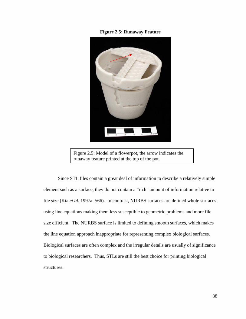
Figure 2.5: Runaway Feature
Figure 2.5: Model of a flowerpot, the arrow indicates the runaway feature printed at the top of the pot.
Since STL files contain a great deal of information to describe a relatively simple
element such as a surface, they do not contain a “rich” amount of information relative to
file size (Kia et al. 1997a: 566). In contrast, NURBS surfaces are defined whole surfaces
using line equations making them less susceptible to geometric problems and more file
size efficient. The NURBS surface is limited to defining smooth surfaces, which makes
the line equation approach inappropriate for representing complex biological surfaces.
Biological surfaces are often complex and the irregular details are usually of significance
to biological researchers. Thus, STLs are still the best choice for printing biological
structures.
38

There are a plethora of 3D file types available today. RP systems primarily utilize
the STL file format, however this format is not capable of representing colour. New RP
systems such as the Z-Corp 3D printers are capable of printing colour. Typically, a
VRML (Virtual Reality Modeling Language) file is used in place of the STL when colour
is required. The VRML file used for RP is a polygonal file similar to the STL that can
encode various types of multimedia information. For example, VRML files can
accommodate colour information within a standard polygon model in the form a regular
image file such as a bitmap (BMP). The VRML is still limited by the same problems
associated with STL files, but also carries the same advantage of representing complex
surfaces.
From the above review of the work on imaging and RP some general trends can
be identified. First, RP is likely the most appropriate manufacturing technology to be
used to recreate biological objects from digital data. In order for researchers in
anthropology to effectively use fabrication technology to create physical replicas of
virtual 3D objects, the approach must be easy to use, cost effective and able to reproduce
both internal and external structures with accuracy at least relative to data acquisition
error. Finally, data acquisition and data processing errors are the most limiting factors in
creating 3D models both virtually and physically.
39

The Role of 3D Printing in Biological Anthropology
Since most uses of RP are limited to case study reports, there is no definitive
guide for researchers looking to integrate this technology into existing projects. This is
partly due to barriers such as cost and cross-disciplinary communication. A more
comprehensive understanding of how RP can be used in biological anthropology is
required for this technology to be used in regular research projects. In order for RP to be
used more frequently than the odd case study, a more thorough understanding of the role
of RP in biological anthropology is also required.
Objectives
The purpose of this work is to explore the role of 3D printing (3DP) in biological
anthropology. Understanding how this technology can be used to enhance our
understanding of biological anthropology requires first understanding three basic
methodological considerations: the types of data acquisition that can be used to create
printable virtual models, how the original object, virtual model and printed model
compare within the scope of the research project, and how the resulting printed model
can enhance our understanding or facilitate the dissemination of research in biological
anthropology. Two case studies will be used to identify these basic methodological
issues and provide a forum for the larger discussion of the role of 3DP in biological
anthropology. These two cases are chosen as a starting point for looking at the potential
for the more common use of 3DP.
The first case study will examine the use of 3DP in reconstruction projects using a
flowerpot. The choice of a flowerpot is intended to evaluate the basic principals of
reconstruction using a simplified object, prior to venturing into more complicated skeletal
40

material. The ability to successfully create a replica of the broken flowerpot will be
evaluated from both the data acquisition and printing perspectives in order to understand
the role of 3D printing in this area of biological anthropology.
The second case study will examine the use of 3D printing for the creation of a
skeletal replica. This case study will look at the differences in model applications related
to methods of data acquisition. Two methods of data acquisition will be used; laser
surface scanning and CT scanning. In evaluating the role of 3D printing in biological
anthropology, it is important to understand the relationship between data acquisition,
processing and printing. The understanding of this relationship is what is lacking in the
case study reports of the more general use of RP in biological anthropology.
Cost and accessibility are two barriers to the regular use of RP in biological
anthropology to date. Ono and colleagues (2000) have suggested that 3DP has the
potential to be effective for anatomical modeling and overcomes the cost barrier reported
by other researchers in relation to the more widely accessible approach of SLA (Dolz et
al. 2000, Hieu et al. 2005, Hjalgrim et al. 1995, Powers et al. 1998). In consideration of
this, 3DP was selected as the primary method for both case studies. A project of this
scale would have been prohibitively costly using the more commonly used SLA
approach.
3D Printing Methods
Z-Corp is the company licensed to manufacture and distribute ‘3D printers’ based
on the binder-jet technology developed at the Massachusetts Institute of Technology
(MIT). As of December 2005, they market three machines. The Z-310 is a small,
economical 3D printer capable of only printing in monochrome. The Z-510 (successor to
41

the Z-406) is a medium sized unit capable of colour and monochrome printing and the Z-
810 is a large format printer also having colour and monochrome capabilities. All of
these machines can use either plaster or starch-based materials for the building medium.
The virtual models were printed using a Z-Corp, Z-406 3D printer. Plaster-based
material and binder solution was used to recreate the 3D objects. A layer of plaster is first
spread onto the build chamber floor. A layer of binding solution is sprayed onto the
powder surface in the shape of a 2D cross-sectional slice of the original object. This
process is repeated until a 3D object is produced within the build chamber. The
maximum build volume for the Z-406 is 203x254x203 millimeters (8x10x8 inches).
Figure 2.6 illustrates the building process from 2D cross-section to partially excavated
object.
Figure 2.6: Z-406 Build Chamber
a b
Figure 2.6: Image “a” illustrates the build chamber of the Z-406 during the printing process. A 2D cross-section of the object is printed by depositing a layer of binding solution onto a bed of plaster. Image “b” represents the printed model partially excavated from the build chamber.
Excess powder is cleaned from the model with a conventional brush followed by an
airbrush. This research used the zp102/zb56 plaster and binder combination with
42

corresponding colour binder (donated by Z-Corp). The layer thickness can be custom set
using the Z-Print software (0.076mm to 0.254mm); the default setting of 0.2 millimetres
was used for this project. Z-Print software version 6.3.28 provided the interface between
computer and printer. The models were all infiltrated using a paraffin wax bath to seal
and stabilize the plaster models.
Case Studies
Each case study has been organized as a stand-alone chapter. Both case studies
use the same 3DP methods described above, but each has a distinct data acquisition and
processing methodology. Chapter III will present the first case study on reconstruction.
Chapter IV will present the case study on creating the skeletal replica. A discussion of
the technical issues of each study is found at the conclusion of both chapters. Chapter V
is a more conceptually oriented discussion of the overall role of 3DP in biological
anthropology. The discussion chapter synthesizes the overall lessons that can be learned
from considering both studies as a representation of the types of applications for 3DP in
biological anthropology.
43

Chapter III: Case Study 1: Virtual Reconstruction
_______________________________________________________________________
Reconstruction of recovered bone and associated material is an important aspect
of some projects in biological anthropology. Reconstructions of fragmented materials
allow researchers to assemble the broken pieces of the past to gain a more coherent
understanding of form and structure. In biological anthropology reconstructions of the
skeleton from ancient peoples can add to the understanding of evolution through
morphometric analysis. In a medical-legal context reconstructions of fragmented remains
can assist forensic investigations. One of the most significant limitations of such
endeavours is the physical manipulation of the remains. Such manipulation can lead to
the permanent destruction of unique and precious material. Virtual reconstruction is
emerging as a potential tool to overcome the problems associated with the physical
manipulation of remains. Virtual reconstruction uses three-dimensional digital
technology to capture the form of objects allowing manipulation and study in a three-
dimensional computer generated environment. 3D printing offers the potential to move
the next step forward and reproduce the virtually reconstructed objects to reflect some
aspect of the reconstruction process or model the original object. Zollikofer and Ponce
de Leon (2005) term this “real virtuality”, whereby virtual representations are converted
back into the form of the original.
44

Objectives
3D printing technology has the potential to extend the role of virtual
reconstructions by offering rapid, low-cost concept modeling and colour layering for
enhanced analysis. In order for this technology to be a valuable analytical tool, several
conditions must be met. First, there needs to be an effective method of reconstruction
that can produce the necessary models for the 3D printing device and the printed objects
must be an accurate representation of the original object. Accuracy for this case study is
the ability to match the physical dimensions and overall surface topology of the original
object within the accuracy limit of the scanning device (1 mm). Finally, the printed
model must offer some advantage for the study or dissemination of the results from the
original material. This study will also evaluate and identify the methodology for using
3D surface scanning to generate the virtual models. A simple flowerpot is used as a
starting point for testing. If a successful reconstruction method can be identified that
satisfies the accuracy and usefulness conditions, the concept will be valid and eligible for
further study using more complex material (for example, skeletal elements).
Methods
Using laser surface scanning a virtual model of a ceramic flowerpot (Figure 3.1)
was created and printed.
45

Figure 3.1 Original Flowerpot
Figure 3.1: From left to right; side , bottom and top views of original flowerpot.
Following the successful creation of a virtual model, the pot was then broken and
reconstructed using surface scan data of the broken pieces. The resulting reconstructed
virtual model was compared to the original virtual model for similarity and printed.
Surface Scanning:
A Polhemus Fastscan™ handheld laser scanner was used for surface scanning.
This scanner uses a laser, camera and motion-tracking system to record a 3D point set of
the original object surface. The laser and range-finding (charge-coupled device or CCD)
camera are contained in a portable handheld wand. A fan of laser light is emitted from the
wand as the user scans the object’s surface using a motion similar to spray painting. The
range finding optics calculate the distance from the object to the scanner and record the
position as a point in 3-space. The motion tracking system establishes these points
relative to a single datum identified as the transmitter 0,0,0. The motion tracking for the
Fastscan™ is based on the Fastrak® system marketed by Polhemus. The Fastrak®
system tracks the position of a receiver (in the wand) in relation to the transmitter (0,0,0)
through a low frequency magnetic field generated by the transmitter. The result is the
46

ability to scan objects with accurate six degrees of freedom (X,Y,Z, Azimuth, Elevation
and Roll). Figure 3.2 illustrates the principals of the Fastscan™ system.
Figure 3.2 Scanning Diagram
Figure 3.2: The scanner operates within the electromagnetic field and the useful range of the scanner is contained within this area (marketed by red circle). The scanner is identified in relation to the object through the reflection of the laser off the object and recorded by the CCD camera contained within the handheld unit. The resulting data are then processed by a computer.
Resolution of the scanner decreases as the distance between the object and wand
increases. Resolution is also affected by the scanning rate (i.e. the speed at which the user
passes the wand over the object). Average resolution is 0.5mm at a distance of 200mm
from the object, where line-to-line resolution is 1mm at a speed of 50mm per second
(pers. comm. Dan Ratta, Polhemus). Since the motion tracking system is based on a field
generated from the transmitter, accuracy depends on wand-object range in relation to the
transmitter. Accuracy for the Fastscan™ is therefore 1mm at a distance of 200mm (pers.
comm. Dan Ratta Polhemus). The limitations of the scanner’s resolution are important to
consider in the context of the printed object. If the smallest feature that the printer can
produce is 0.76 mm (Grimm 2004), then the printer is capable of printing a finer object
47

than can be imaged using the Polhemus scanner. In this case the limitation on the
reproducible amount of detail is with the method of data acquisition.
The pot was scanned upside-down on a black felt cloth. Felt absorbs all the light
from the laser, eliminating the capture of background surfaces. It was not possible to
accurately scan the inside surface of the pot. The angle of the camera and laser was too
wide to capture the detail within the narrow opening of the pot (Figure 3.3).
Figure 3.3: Camera and Laser Angle for Optimum Scanning
Scanner
Figure 3.3: Red arrows indicate the triangulation pattern between the camera’s line of sight and the light emitted from the laser. The blue circle shows the scanning area possible. Note that the circle is offset, meaning that the scanned area within the pot could be manipulated by changing the angle of the handheld device.
Rather than capturing only some of the surface data inside the pot and filling holes, the
outside was scanned and the inside surface was approximated from this data during
model post-processing. The scan was exported from the Fastscan™ as an STL file. Post-
processing involved two different methods. Each method has advantages and
disadvantages. Analyzing these results will provide a better understanding of the most
appropriate post-processing methodology for virtual modeling and for 3D printing.
48

Virtual Modeling of Unbroken Flowerpot
The virtual modeling of the unbroken flowerpot examined two different post-
processing methods. Procedure one involved first filling holes using the automatic
function in the RapidForm™ software. The hole filling resulted in irregular surfaces,
corrected by using the smoothing function. The inside surface of the pot was estimated by
giving the shell (surface model) a surface thickness of 3mm using the “volume” function
in RapidForm™. Once the model was visually acceptable, an automated cleaning
function was executed to find and repair problems in the geometry that were not visually
apparent (crossing faces, unstable faces, non-manifold faces and vertices with redundant
faces). This automated algorithm for cleaning the problem geometry was not able to
remove all the errors in the model, although it did result in a printable model. It actually
increased the number of non-manifold faces from 1554 to 1766, redundant vertices from
744 to 870 and crossing faces from 166 to 398; but decreased the number of unstable
faces from 1395 to 0. Figure 3.4 below shows the result of post-processing method one.
49
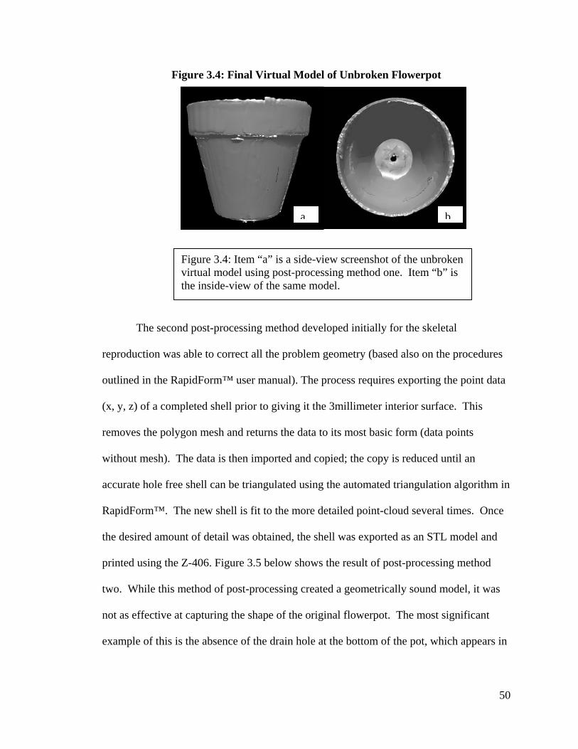
Figure 3.4: Final Virtual Model of Unbroken Flowerpot
a b
Figure 3.4: Item “a” is a side-view screenshot of the unbroken virtual model using post-processing method one. Item “b” is the inside-view of the same model.
The second post-processing method developed initially for the skeletal
reproduction was able to correct all the problem geometry (based also on the procedures
outlined in the RapidForm™ user manual). The process requires exporting the point data
(x, y, z) of a completed shell prior to giving it the 3millimeter interior surface. This
removes the polygon mesh and returns the data to its most basic form (data points
without mesh). The data is then imported and copied; the copy is reduced until an
accurate hole free shell can be triangulated using the automated triangulation algorithm in
RapidForm™. The new shell is fit to the more detailed point-cloud several times. Once
the desired amount of detail was obtained, the shell was exported as an STL model and
printed using the Z-406. Figure 3.5 below shows the result of post-processing method
two. While this method of post-processing created a geometrically sound model, it was
not as effective at capturing the shape of the original flowerpot. The most significant
example of this is the absence of the drain hole at the bottom of the pot, which appears in
50

the virtual model using processing method one (Figure 3.4), but not the new procedure
(Figure 3.5).
Figure 3.5: Unbroken Flowerpot Post-processing Method 2
a b
Figure 3.5: Item “a” is a side-view screenshot of the unbroken virtual model using post-processing method two. Item “b” is the inside-view of the same model.
Virtual Reconstruction of Broken Flowerpot
Following the successful virtual modeling of the original unbroken flowerpot, the
pot was broken into 5 principal pieces (Figure 3.6).
Figure 3.6 Broken Flowerpot
Figure 3.6: Five broken pieces of the flowerpot. The red circle highlights debris that was too small to be effectively scanned.
51

The five pieces were individually scanned using the Polhemus laser scanner. All the
pieces were scanned on the black felt with the outer surface facing upwards. Each shard
was exported directly from the Fastscan™ software in STL format. RapidForm™ was
used to put the pieces back into the shape of the original flowerpot.
Figure 3.7: Shard Models
Figure 3.7: Single-sided virtual models of the individual shards organized from smallest to largest (left to right) and magnified for clearer view.
Two approaches to the reconstruction of the flowerpot were evaluated. In order to
maintain continuity between the modeling of the unbroken and modeling of the broken
pot, only the outside surface was scanned. The inner surface was approximated by
thickening the shell by three millimetres as per the making of the unbroken virtual model.
52

Figure 3.8: Thin Shard to Thick Shard
a b
Figure 3.8: Example of shard prior to thickening (a) and after thickening (b). Note the red lines in “a” represent the edges of overlapping scans, an artifact of the scanning process.
The first approach to the reconstruction joined the shards after they were
thickened. Adding the other side to the shards increased the amount of irregularity in the
attachment surfaces, which made accurate matching very difficult (note the raised edges
of 3.8-b). Several large gaps were also present between some of the matched pieces (see
Figure 3.9). The hole-filling algorithm in RapidForm™ was not able to fill these gaps.
The hole-filling tool is intended to repair gaps defined by boundaries. Boundaries are
mathematically defined edges of the polygon shell (red lines depicted in Figure 3.8-a).
Since the individual pieces were solid-volumes and the boundaries only defined the edges
of the surface model, the software recognized the holes on the surface and not the gaps
between the shards. A rough model was created using this method of reconstruction
(Figure 3.9).
53

Figure 3.9: Reconstruction Using Volume Shards
a b
Figure 3.9: Side-view (a) and top view (b) of reconstructed pot using method one.
The second method combined the pieces as single-sided shells and added the
inside surface of the model once the pieces were registered together. The second
reconstruction method based on the “thin wall registration” function in RapidForm™ was
used to produce the most successful reconstructed virtual model. The pieces were fit
together prior to making them into volume entities. This function required selecting three
points on one shard and another three corresponding points on the adjoining shard as seen
in Figure 3.10.
54
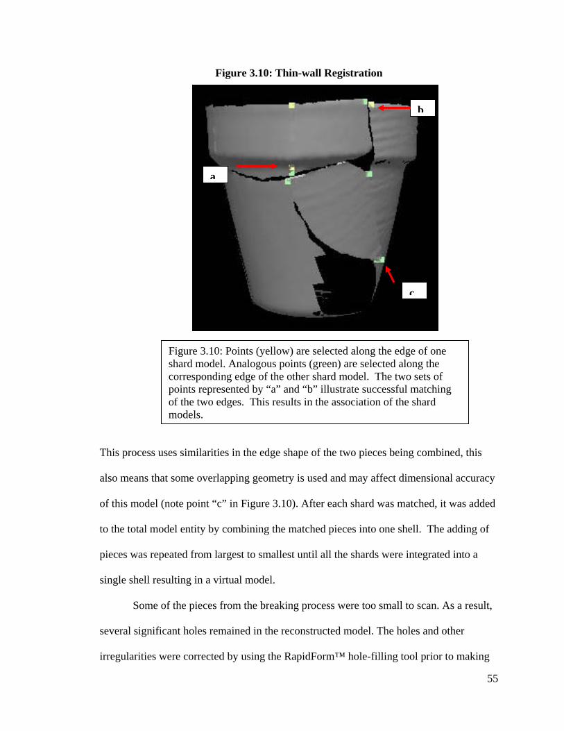
Figure 3.10: Thin-wall Registration
b
a
c
Figure 3.10: Points (yellow) are selected along the edge of one shard model. Analogous points (green) are selected along the corresponding edge of the other shard model. The two sets of points represented by “a” and “b” illustrate successful matching of the two edges. This results in the association of the shard models.
This process uses similarities in the edge shape of the two pieces being combined, this
also means that some overlapping geometry is used and may affect dimensional accuracy
of this model (note point “c” in Figure 3.10). After each shard was matched, it was added
to the total model entity by combining the matched pieces into one shell. The adding of
pieces was repeated from largest to smallest until all the shards were integrated into a
single shell resulting in a virtual model.
Some of the pieces from the breaking process were too small to scan. As a result,
several significant holes remained in the reconstructed model. The holes and other
irregularities were corrected by using the RapidForm™ hole-filling tool prior to making
55

the shell a volume. Since the shell is represented as a single surface, the edges are defined
by boundaries. The boundaries therefore defined the holes on the surface of the shell and
were filled. Unlike the earlier volume model, in this case, the model consisted of only
the outer surface. Following the hole-filling procedure, extensive smoothing was
required. Automatic filling of the largest hole resulted in a major deformity from the
surface, which was necessary but difficult to correct. The top of the pot was also very
irregular and required cropping and smoothing. Figure 3.11 illustrates the before and
after result of smoothing and cropping the model.
Figure 3.11: After Hole Filling and Smoothing
a b
Figure 3.11: Image “a” depicts the pot with bulging deformity on the bottom and extended brim. Image “c” shows the result of the smoothing and cropping process.
After the above-mentioned processing was completed, the model was then thickened by 3
mm to approximate the inner surface. This resulted in the final model that was exported
to he printer as an STL file (Figure 3.12).
56

Figure 3.12: Final Virtual Model Using Reconstruction Method Two
ba
Figure 3.12: Side-view (a) and top-view (b) of virtual flowerpot model based on reconstruction method two.
A third model was also created, which synthesized method two with post-
processing method two used for the unbroken pot (simplification, detailing and cleaning).
This last model was created in order to overcome problems with the geometry of the
reconstructed pot models. The process of combining models together to make a single
entity causes the development of many crossing faces, redundant faces and inappropriate
boundaries. The result of using post-processing method two produced a smoother more
refined surface finish for both the unbroken (a) and reconstructed (b) pots, as seen in
Figure 3.13.
57

Figure 3.13: Virtual Models of Unbroken and Reconstructed Flowerpots
a b
Figure 3.13: Side-views of both the unbroken virtual model (a) and the model created using reconstruction method two (b), using post-processing method two.
Once the virtual models were ready, they were imported into the Z-Print
software that interfaces with the Z-406 printer. The first models were printed at 70
percent of their original size to reduce overall material cost. The model from
reconstruction method one was not printed due to the poor quality of the virtual model.
The following figures (3.14 to 3.18) depict the results of the printed models by each
method.
58

Figure 3.14: Unbroken Model Using Post-Processing Method One
a b
Figure 3.14: Images “a” and “b” show top facing side-view and bottom facing side view respectively. Red arrows mark imperfections in the rim of the pot and the detail of the drain hole.
Figure 3.15: Unbroken Model Using Post-Processing Method Two
a b
Figure 3.15: Image “a” illustrates the top facing side view and image “b” shows the bottom facing side view. Note the red arrow marks the absence of the drain hole detail in this model, but the surface is smoother.
59

Figure 3.16: Reconstructed Model Using Method Two
Figure 3.17: Reconstructed Model Three (Combined Methods)
a b
Figure 3.16: Images “a” and “b” depict the top facing and bottom facing side views respectively. Areas of surface imperfection are circled in red. The arrow points out the absence of the drain hole detail.
ba
Figure 3.17: Images “a” and “b” depict the top facing and bottom facing side views respectively. The red arrow in image “a” highlights the thin plate that formed inside the top of the pot. The arrow in image “b” illustrates a geometry imperfection (crossing face) likely related to formation of the unwanted structure in image “a”.
60

Results
The intention of this work is to move beyond testing just the linear accuracy of
the printer. Therefore, the following analysis examines the dimensional and
topographical accuracy of the overall process from original to printed object. It is
however, necessary to establish a base-line understanding of where to expect the greatest
amount of dimensional error in the overall process. In order to do this, a 1:1 scale model
of the unbroken flowerpot (using post-processing method two) was printed and compared
to the original and virtual models from each of the processing and reconstruction
methods. Height was measured from the base of the pot to the top of the rim, parallel to
the side . Maximum external width was measured from the top rim of the pot. The
virtual models were all measured in RapidForm™. The results of these measurements
are summarized in Table 3.1.
Table 3.1: Original and Printed Pot Comparison
Pot Version
Measurement Original
Virtual Unbroken Method One
Virtual ReconstructionMethod One
Virtual Unbroken Method Two
Virtual Reconstruction Printed Method Two Unbroken
Height (cm) 9.75 10.00 10.12 10.00 10.00 10.50Width (cm) 14.50 11.01 10.07 11.14 11.34 11.20
The above measurements provide a quick overview of where the largest challenge
exists for recreating a dimensionally accurate model. Height is the most accurate
distance between all the models, with the printed model showing the greatest difference
(+0.75 cm). Some of this difference is seen in the move from the original to the virtual
model by an inflation of 0.25 cm (held by three of the four virtual models). The
remaining 0.5cm difference appears to be the result of accuracy between the virtual
61

model and printing process. The pot was printed upside down in the build chamber to
prevent excess pressure from the loose plaster within the walls of the pot, when being
excavated. This also means that the dimension of height corresponds to the z-axis during
the printing process. The z-axis has the most significant amount of error during the
printing process due to the layering of the cross-sections in 0.2-millimeter thicknesses. If
the pot were printed with a different orientation inside the build chamber, the height
dimension would likely be affected.
The greatest amount of overall difference is seen in the width measurements, with
the majority of the discrepancy being between the original and virtual models. The
difference between the original and four virtual models is around three centimetres. The
difference in width between the original and the virtual model that the printed version is
based on is 3.16 cm. In contrast, and with the exception of virtual reconstruction method
one, the virtual models are all within a few millimetres in width. The difference in width
between the virtual and printed model is 0.14 cm (or 14 mm). This clearly illustrates that
the problems in the width dimension originate in the virtual modeling process and not the
printing process. This is consistent with what is expected of the printer given that the
width of the printed pot is determined on the x and y axes, which are known to be the
most accurate.
This simple and relatively quick assessment of dimensional accuracy in the
modeling process from original to printed model has pointed out two important issues.
First, the orientation of the printed object within the build chamber is a significant
determinant of dimensional accuracy. Every effort should be made to limit the amount of
printing on the z-axis. Secondly, a greater amount of error is seen between the original
62
pot than amongst the virtual models. This confirms an earlier assumption that the method
of data acquisition (in this case laser scanning) contributes the most to accuracy
problems. This may be due to the actual limitations of the scanner, but is also likely due
to the extent of post-processing required to generate a 3D model from point data. The
accuracy of the scanner is based on the ability to record individual coordinate data from
the surface of the object in the form of a point-cloud. The virtual model results from a
complicated algorithm and editing process to generate a meshed surface from this
coordinate data.
An analysis of the overall surface shape differences between the complete and
reconstructed virtual pots was performed using RapidForm™. This process involved first
registering the two virtual models to a common set of coordinates and datum. This
allows the software to measure the distance between the models by each coordinate (x,y
and z) in relation to the common datum point. The results of this analysis can be
displayed graphically with colour coding to illustrate areas of difference, or by exporting
the actual displacement values to a spreadsheet program for further analysis. This
inspection process was tested for validity by performing the inspection on the same
model. The result was a deviation value of zero, suggesting that real differences can be
observed using this method.
Only the unbroken and reconstructed virtual models that were post-processed
using method two could be registered using the RapidForm™ inspection process. The
other models had far too many geometry problems to be accurately registered. Twisted
geometry is a particular problem as registration is only effective if all the vertices are
63

oriented to the same plane of reference. Table 3.2 summarizes the displacement of
common vertices between these models based on 11,328 coordinates.
Table 3.2: Unbroken and Reconstructed Differences (mm)
Variable X Y Z Total MEAN 0.02 0.00 0.05 -0.19 ST. DEV. 0.31 0.30 0.23 0.45 MIN. -1.34 -1.96 -3.55 -1.93 MAX. 2.61 1.52 1.27 3.64
Coordinates on the X-plane show the greatest amount of difference and variation. The
total variation for all points ranges between -1.9mm and +3.6mm. The range of variation
can be limited to a specific set of values with a colour map displaying the variation over
the 3D shape of the object. Figure 3.18 and 3.19 show the deviation of the reconstruction
as compared to the unbroken virtual model between the values of –1 and +1 millimetres.
64

Figure 3.18: Side View of Flowerpot Inspection Results
Figure 3.18: This image represents a colour-coded model of the deviation in coordinate values between the unbroken and reconstructed models. The values are expressed as a relationship between the deviation of the reconstruction from the unbroken model. The blue represents negative values to a limit of –1-mm (see scale) and positive values to a limit of +1-mm (see scale). The dominance of the blue colour indicates that the reconstruction is primarily smaller than the unbroken model.
65

Figure 3.19: Top/Inside View of Flowerpot Inspection Results
Figure 3.19: Same model and display values as Figure 3.19. This view shows the extent of variation on the inside surface. From this image it is possible to understand the variation in the topology between the models. The rim is particularly variable, differing by both positive and negative values. As well, there seems to be several localized and random areas of variation. Again, the dominance of the colour blue indicates that the reconstruction is smaller than the unbroken model.
Larger values failed to show shape differences and displayed the model in a solid blue
colour, which corresponded to an overall negative dimensional relationship between the
unbroken and reconstructed models. This makes sense since Table 3.1 shows that the
66

unbroken virtual model in this case is smaller than the reconstructed model. Tightening
the limits allows for the display of the variation in surface topology.
Discussion
The result of this inspection process indicates that despite some heavy variation
around the rim of the pot, the topological difference between the models is relatively
minor. Figure 3.18 shows some regular variation along the outer surface that corresponds
to a pattern of surface dimpling. While somewhat uniform, this variation could
disqualify the reconstruction as an accurate representation of the shape of the unbroken
model in a strict sense. In this case, the purpose of the reconstruction really should
dictate the decision to accept or reject the validity of the reconstruction.
It is important to frame the decision of whether or not the reconstruction of the
flowerpot was successful within the context of the end goal. The issue with any
reconstruction, especially of the past, is that it is difficult to know how exact the
reconstruction is to the original. If a general likeness in size and shape is the only
requirement, then the above reconstruction was successful. If more detail is required to
understand changes in shape of the surface (as would be required for evolutionary studies
or forensic applications), then this reconstruction effort was not successful. A
particularly problematic issue is the absence of the drain hole, which was only
reproduced in the virtual model of the unbroken pot using post-processing method one.
Post-processing method two yielded a geometrically sound model, but destroyed much of
the individualizing elements of the original flowerpot. Also important to note is that
width changed more than height between the original and virtual models (particularly the
reconstructions). This means that overall shape also changed.
67

There is an alternative usefulness for the 3D printer to reproduce virtual
reconstructions. The colour capabilities of the Z-406 allow for the communication of
differences in design and reconstruction iterations, through a tangible object that can be
directly compared to the original. The unbroken and reconstructed models where given
opposite colours (red for the unbroken and blue for the reconstruction), and registered
using the same approach as the inspection process. The models were then saved as a
single model and exported to the printer for printing. The result was a printed colour
model of the absolute differences between the models that could be handled and
examined in association with the original or other material. Figure 3.20 illustrates the
resulting model.
Figure 3.20: Colour Model of Flowerpot Differences
a b
Figure 3.20: Image “a” and “b” illustrate the top facing side view and bottom facing side view of the colour differences model respectively.
The above colour model illustrates the beginning of a new level of communication
possible using colour 3D printing. This type of colour modeling may also help museums
disseminate the limitations of reconstructions and be used to highlight differences in
68

interpretations of the past, and could apply to either biological specimens or material
culture.
Conclusion
The sum of the results in this section indicates some clear issues that need to be
considered for the reconstruction project. First, despite the problems associated with
accuracy of printing on the z-axis, there is good agreement between the virtual and
printed models. The problem lies with the post-processing of the original data and the
overall reconstruction approach. As seen in the elimination of the drain hole in the
unbroken virtual model using post-processing method two, extensive editing erodes a
great deal of the surface detail. Not processing enough introduces other quality issues
relating to geometry problems that translate into surface quality issues in the final printed
object. A more accurate method of reconstruction is required for future studies as well,
especially those involving more complex material. It is conceivable that an acceptable
reconstruction could be printed using a more accurate reconstruction method and data
that requires less manipulation than the surface scan data. A possible way to mitigate
these problems would be to use CT data, which may require less manipulation to create
clean models. A test of this hypothesis is carried out in case study two using skeletal
material.
69

Chapter IV: Case Study 2: Skeletal Reproduction
________________________________________________________________________
Objectives
The focus of this case study is to build upon and test the methodological concepts
developed in Case Study One on actual skeletal material. Case study one showed that
extensive post-processing of scan data is required for the creation of printable virtual
models of a flowerpot (unbroken and reconstructed). This led to the conclusion that
extensive post-processing of the raw data reduces the degree of analysis possible with the
virtual models or printed objects. CT scanning was proposed as an alternative method of
data acquisition, which may provide a solution to the limitations identified for the surface
scans. This proposal is evaluated using case study two by attempting to reproduce an
entire skeleton using both laser surface and CT scanning methods of data acquisition.
Case study two has two components: first, an evaluation of the use of laser surface
scanning and 3D printing to create a replica of an entire skeleton, and second an
evaluation of the use of CT scanning as an alternative method to laser surface scanning of
skeletal material. As well as illustrating the technical limitations of each data acquisition
method, a procedure for developing printable models of skeletal material will be
highlighted for future use by other researchers.
Each approach to data acquisition will be compared in relation to the degree of
usefulness of the resulting physical models. Usefulness is contextualized through three
specific applications relating to research in biological anthropology:
1. Application of the physical models for general education.
2. Application of the physical models for the dissemination of research.
70

3. Potential for using physical models in traditional osteological analysis.
Usefulness of the resulting models relates to the overall goal of this work, which is to
discuss the role of 3D printing in biological anthropology. Part of understanding this role
is knowing what methods of data acquisition should be used to accomplish the specific
goals of any given project in biological anthropology.
Materials
The Mennonite Heritage Village Museum (MHV) wanted to incorporate a replica
of an early Mennonite skeleton as part of a larger exhibit entitled “New Life”, describing
funerary practices of Mennonite settlers in Manitoba, Canada. Myra Sitchon, a doctoral
student at the University of Manitoba originally proposed using laser surface scanning to
make 3D virtual models of a skeleton for this exhibit (Sitchon et al 2004). The skeleton
of interest to the MHV is thought to be a woman who lived during the 1800’s and early
1900’s from the former Schoenfeld village in southeastern Manitoba. The remains were
archaeologically recovered in 1995 and have been analyzed by Dr. Deborah C. Merrett
and Dr. Chris Meiklejohn at the Department of Anthropology, University of Winnipeg.
This skeleton is complete but very fragile with some broken elements. In some areas,
patches of cortical bone have flaked off exposing the trabecular bone underneath. Heavy
soil staining is also found on most bone surfaces. Myra Sitchon introduced the idea of
using a non-invasive means of reproduction, such as 3D surface scanning, to overcome
the difficulties of reproducing the fragile skeleton using traditional means (such as
casting, which was totally unacceptable due to the fragility of the material).
71

Methods
Laser Surface Scanning
The laser surface scanning was accomplished using the Polhemus Fastscan™ and
took place at the University of Winnipeg, Anthropology Laboratory where the skeleton is
curated. A laptop computer was used to run the Polhemus software and all the scan files
were saved in STL format. In order to capture all the surfaces of each bone, a specific
scanning procedure was used. Each bone was scanned multiple times: one scan covered
the distal or inferior aspect, another covered the proximal or superior side. In some cases
a third or fourth scan was required from an alternate perspective. The goal of this
scanning procedure was to generate multiple scans that could be stitched together using
the post-processing software. This also meant that all the scans of a given bone required
sharing some geometry in common. This gave the software a reference point for
merging, or registering the scans to make a complete model. Figure 4.1 illustrates the
concept of multiple scans.
Figure 4.1: General Scanning for Bones
72
Figure 4.1: Scan one covers the distal epiphysis to the metaphysis of the long bone. Scan two covers the proximal epiphysis and metaphysis. Note the critical overlapping scan region that yields the common geometry necessary for the registration of the two scans to make a complete bone model.

A total of fifty-seven skeletal elements were surface scanned. Soil staining and
erosion of the cortical bone leading to the exposure of the underlying trabeculae made
scanning some items challenging or impossible. Problems associated with soil staining
could be partially compensated for by adjusting laser intensity, since the darkly stained
areas absorbed more light than non-stained areas. Higher intensity values were used for
stained areas; the laser could then be turned down on the fly after passing over the stained
areas. Several vertebrae could not be scanned due to a combination of feature size,
staining and cortical bone erosion (cervical 1 through 7, thoracic 1 through 7 and lumbar
1 through 3). The three cuneiforms for both the left and right feet were also too small
and too stained to yield effective scans. The ribs were significantly stained with extensive
cortical erosion making their structure weak and difficult to handle. Any elements too
fragile to handle were not scanned. Only 10 of the 24 ribs were preserved well enough to
be handled without damage during the scanning process. The time constraint placed on
the skeletal reproduction necessitated reducing the number of scans when possible,
therefore only the right metatarsals and right metacarpals were scanned. The most
significant limitations to successful scanning were size of the bone (too small) and
fragility. Table 4.1 summarizes the scanned elements along with the number of scans and
their orientation, required to complete the model.
73

Table 4.1: Surface Scan Summary
Element Number of Scans Scan Orientation Sacrum 4 Proximal, Distal, Superior, Inferior Mandible 2 Anterior/Superior, Posterior/Inferior Skull 4 Proximal, Distal, Superior, Inferior Sternum 4 Proximal, Distal, Superior, Inferior Vertebrae T8 to T12 2 Superior, Inferior Vertebrae L4 & L5 2 Superior, Inferior Calcaneus (L & R) 2 Proximal, Distal Talus (L & R) 2 Proximal, Distal Tarsals (2) 2 Proximal, Distal Metatarsals (5) 2 Proximal, Distal Femur (L & R) 2 Proximal, Distal Fibula (L & R) 2 Proximal, Distal Patella (L & R) 2 Proximal, Distal Tibia (L & R) 3 Proximal, Distal, Inferior Diaphysis Pelvis (L & R) 2 Superior, Inferior Clavicle (L & R) 2 Proximal, Distal Metacarpals (5) 2 Proximal, Distal Humerus (L & R) 2 Proximal, Distal Radius (L & R) 2 Proximal, Distal Scapula (L & R) 4 Proximal, Distal, Superior, Inferior Ulna (L & R) 2 Proximal, Distal Ribs (10 scanned) 3 Proximal, Distal, Shaft Total: 57
Image processing of the surface scan data was undertaken using the RapidFormTM
software. The editing process followed a series of steps: registration, simplification,
detailing and cleaning (a method suggested in the RapidForm™ user manual). This
method was required to overcome the problems associated with generating models of
skeletal material, which have a complex surface morphology. Surface scans collect a
series of points representing the object; these points are then made into a surface mesh
using an automated algorithm. Object complexity increases the chance that the algorithm
74

will make errors in the calculation of the surface mesh. The above-mentioned procedure
overcomes this difficulty by reducing the complexity of the data prior to generating the
surface mesh and then adding the detail back to the simpler surface.
In order to cover all surfaces of each bone, multiple scans were taken. The first
step in processing the scan data to make a model was to register the multiple scans of
each bone together. The software uses common geometry between two scans to estimate
the best fit. The identification of the common geometry is user directed by selecting four
points that corresponded to common areas between two scans of a single element and
executing a registration function (note the overlapping scans in Figure 4.1). The
registration function aligns the two scans together based on this input and combines the
scans into one. The result is a model file of the entire bone. The matching requires the
user to visually judge areas of similarity between the two scans. Working with meshed
surfaces such as the STL files exported from the scanner makes this process a great deal
easier. It is possible to use the unmeshed point cloud data, but that makes identifying
areas along the surface very difficult since there is no visual reference for the surface,
only a series of points. The registration process is explained graphically in Figures 4.2
and 4.3.
75

Figure 4.2: Registration Process Step One
b a
c
Figure 4.2: Image “a” shows the unregistered view of the inferior scan and the superior scan of the right innominateinnominate. The scans are separated into viewing windows “b” and “c”. Red, blue and green dots represent the user specified common areas of geometry. These do not need to be exact, as the software uses the curvature of the model’s surface in that area to more accurately match the scans.
76

Figure 4.3: Result of Registration
Figure 4.3: Illustrates the result of the registration process. The colour-coded dots are arranged in groups corresponding to similar geometry between the two scans. The scans are thus oriented correctly, yielding a whole model of the right innominate.
The model file resulting from the registration process is exported as a point cloud
file for the simplification process. This removes the polygon mesh from the shell. The
file is then reloaded under a new project window as a point set. An exact copy of this
point cloud is made and the object is reduced in complexity from the copied point-cloud.
This reduced point-cloud is then re-triangulated using the automatic algorithm in
RapidForm™. Figure 4.4 illustrates the simplification process.
77

Figure 4.4: Simplification
a b
Figure 4.4: Image “a” shows the result of removing the polygon mesh from the model file generated in Figure 4.3. Note the density of the points giving the model an almost solid appearance. Image “b” shows the result of reducing the point-cloud several times until the points represent the basic outline of the shape of the original model.
The simpler model is then re-triangulated using the automated algorithm in the
software. Any resulting holes are filled at this stage of the process to ensure the model is
completely sealed and has no boundaries. Once this is achieved, the detail is added to the
simple shell by fitting the original point-cloud to the surface over several iterations. This
replaces some of the lost detail while maintaining the geometric soundness of the simpler
model. Unfortunately, this also adds a great number of polygons to the surface mesh
increasing the overall file size of the model. A decimation algorithm was then used to
reduce the number of polygons without noticeably affecting surface quality. Figure 4.5
illustrates the process of adding detail to the simplified shell.
78

Figure 4.5: Model Detailing
a b
Figure 4.5: Image “a” is the simplified surface model. Image “b” illustrates the result of several iterations of the detailing process.
Once the re-detailed model is decimated to reduce the file size while maintaining
surface quality, it is exported as an STL. The STL file is imported into the Z-Print
software and printed. All the skeletal elements were oriented so that the least amount of
printing was done on the z-axis of the build chamber. For example, the length of a
humerus would be oriented along the x or y axes, and the width was oriented along the z-
axis.
79

CT Scanning
CT scanning was undertaken at the Department of Radiology, Winnipeg Sick
Children’s Hospital. The material was scanned using a Toshiba Asteion™ multi-slice CT
scanner at 1-millimeter slices, with 0.5-millimeter convolution. A board was placed on
the surface of the scanning table and the skeletal material was grouped into a series of
five scans.
Figure 4.6: Series One
Figure 4.6: Mimics screen-grab of the layout of scan one: cranium, mandible, left and right scapulae, left and right clavicle.
80

Figure 4.7: Series Two
Figure 4.7: Mimics screen-grab of scan two: cervicel vertebrae (1 through 7), left and right humerus, left and right radii, left and right ulnae.
Figure 4.8: Series Three
Figure 4.8: Mimics screen-grab of scan series three: thoracic vertebrae (1 through 12) and sacrum.
81

Figure 4.9: Series Four
Figure 4.9: Mimics screen-grab of scan series four: left and right innominates, lumbar vertebrae (1 through 5).
Figure 4.10: Series Five
Figure 4.10: Mimics screen-grab of scan series five: left and right carpals and metacarpals.
82

During the scanning process, the left clavicle and right innominate were
incorrectly positioned. This resulted in a portion of these two elements being cut off and
not completely recorded. Unfortunately this error was noticed only after the images were
processed from raw files into DICOM and delivered to the researcher. This problem is
illustrated in Figure 4.11.
Figure 4.11: CT Position Error
a b
Figure 4.11: Images “a” and “b” are not related by scale. The red circles in both images “a” and “b” mark the positional error where the bone has not been completely imaged due to being positioned outside of the field of view of the CT scanner.
A total of 65 elements were successfully CT scanned for this project. The scanning took
approximately 3 hours. During the scanning process, the CT equipment needed to be
cooled periodically. This added to the total scanning time.
The CT images were processed using the medical imaging software Mimics.
Mimics converts the DICOM images into a proprietary format and displays three
different views of the subject material (axial, coronal and sagital). This gives the
researcher the ability to edit structures while relating the process conceptually to the
overall 3D perspective of the subject. A project management window uses a system of
83

“masks” (colour coded projects) to organize the editing process. The colour coding
between the mask and object in the three image planes is coordinated.
Figure 4.12: Working in Mimics
c a
b
Figure 4.12: Provides an overview of the work process in Mimics. The different views (axial, coronal and sagatal) are marked “a”, “b” and “c” respectively. The project management window is marked with a red circle.
The skeletal elements were made into virtual models by first selecting an average
threshold of Hounsefield values between –450 and +1637 for the material used in this
project. In general, this range captured the detail of each element in each scan series. The
skeletal elements were then separated from the board by deleting several slices of the
board holding the elements and applying the “region-growing” function to the undeleted
slices. This tool classifies all the connected pixels within the identified threshold value as
a single region of interest over the entire stack of images. The board and the skeletal
84

material are then classed as separate entities and are given distinguishing identities in the
project management window, and corresponding colour coding in the image-plane
windows. Since no soft-tissue was present, the remaining elements were individually
isolated using the same region-growing function and were assigned their own colour
coded identities (Figure 4.13). The individual elements were then exported as STL files
and loaded into the Z-406 for printing.
Figure 4.13: Segmented Elements
Figure 4.13: Different coloured entities depict the result of the region growing process to isolate the individual skeletal elements. From this stage, each bone can be exported as a separate 3D model.
85

3D Printing Whole Bones
The orientation of bones was a significant point of consideration in the printing
process (as per Case Study One), since the z-axis is where the greatest amount of printing
error and the lowest amount of part strength occurs. Therefore, it is important to orient
long thin bones to maximize the x-y plane. To save time multiple bones were loaded into
a single build series since the speed of the printer is mainly limited by the number of
times the gantry can move across the build chamber (six layers per minute in
monochrome and two in colour mode), the most efficient use of time and space involves
limiting the z-axis depth of items as much as possible in the build chamber. The printed
object needed to be left for several hours before removing. This allowed the binding
solution to dry and cure. While in theory, objects can be removed immediately, for this
project objects were left for at least 5-6 hours.
Large bones, such as the Femora and Tibiae, were printed as two segments due to
the limited size of the build chamber in the Z-406 (8 inches wide and 10 inches long).
This meant that these elements also needed to be glued together. The best technique for
this involved beveling the circumference of the adjoining shaft surfaces to provide a
channel for the cyanoacrylate (CA) when the two portions are held together. The CA was
first applied to both adjoining surfaces, and held together until slightly firm (Figure 4.14).
Additional glue was applied through the beveled channel to increase the seal between the
surfaces.
86

Figure 4.14: Joining the Proximal and Distal Femurs
a b
Figure 4.16: Image “a” shows the metaphysial surfaces of the proximal and distal femur. The red arrows indicate where the CA was placed prior to putting the ends together. Image “b” illustrates the joined surfaces; the red arrow marks the beveled edge. CA is placed along this channel as well and later sealed with the powder and binder putty.
The original virtual models were bisected on an angle to increase the surface area for
gluing. Excess CA changes the surface colour of the model and must be covered
appropriately to hide the gluing process. To fix this problem a putty was made with the
plaster and binder solution and applied to the beveled channel. The rough edges were
sanded. This process was repeated until the seam was barely visible. Figure 4.15
illustrates the result of this process.
87

Figure 4.15: Completed Long Bone
Figure 4.15: This femur illustrates an example of the joined procedure used for long bones that did not fit in the build chamber. The red box highlights the area that was filled with the putty and sanded for smoothness. Note: the seams are only visible upon very close inspection of the actual printed object.
The final stage for the entire model collection involved submersion into a paraffin wax
bath.
Results
The principal reason for printing models created using both laser surface scanning
and CT scanning is to evaluate the degree of difference in virtual models between each
acquisition method. This will add to the understanding of the differences and limitations
of surface laser and CT scanning. Eleven of the surface and CT scan models were
compared for differences in shape using RapidForm™. The inspection process was similar
to the one used to compare the unbroken and reconstructed pots in the first case study.
The surface and CT scans of each bone were first registered together using the
88

registration function in the Inspection workbench of RapidForm™. This method
compares both models as if they are the same, by registering them to a common datum
point in three-space. The total number of vertices (and thus polygons) was reduced
equally for both the surface and CT scans after registration using the decimation
algorithm in the software. The two models contained too many points of data for the
software to operate. There was no change in the overall appearance of any of the models
following the decimation procedure, as this algorithm is designed to remove redundant
data points without significantly affecting the overall surface quality of either model.
Following the decimation procedure, RapidForm™ was used to calculate the
displacement between vertices (x, y, z coordinates) and the results were exported to an
Excel spreadsheet for analysis. The surface scan data was compared to the CT data as
though the CT data was the standard; therefore, results reflect the difference of the
surface scan data in relation to the CT data.
Table 4.2: Total Deviation Between Surface and CT Scan Data (mm)
TOTAL VALUES
ELEMENT MEAN ST DEV MIN MAX Total Range
Left Innominate -0.63 0.78 -5.35 4.06 9.41
Left Scapula -1.44 0.51 -4.48 4.15 8.63
Left Humerus -0.24 1.00 -3.40 3.36 6.76
Right Clavicle -0.26 0.83 -2.02 5.01 7.03
Right Humerus -0.98 1.05 -5.24 7.12 12.36
Right Radius -0.71 0.78 -2.49 2.85 5.34
Right Ulna -0.96 0.87 -5.45 2.33 7.78 Right Scapula -1.01 1.44 -7.31 4.35 11.66 Skull -0.74 1.15 -4.96 7.62 12.58
89

While the linear statistical analysis (in Table 4.2) of the comparison between
acquisition methods is limited, it does identify basic trends in the differences between the
models resulting from the two methods. All but two of the means for total variation are
negative values. This suggests that overall the CT data is larger than the surface scan
data. The two outliers for this trend are the left clavicle and right innominate. Both of
these CT scanned items are missing portions due to improper placement on the CT table
during the scanning process and they were removed from the inspection analysis. Figure
4.16 depicts the missing portion of the left clavicle from the CT scan (blue), versus the
surface scan (red).
Figure 4.16: CT vs. Surface Scan for Left Clavicle
Figure 4.16: Red represents the laser surface scan and blue represents the CT scan. Note that the CT scan model is noticeably larger than the surface scan model.
The head of the right humerus was held to the shaft by tape. The discontinuous junction
between the affixed humeral head and diaphysis created significant problems during
triangulation of the surface scan data that necessitated removing that portion. The CT
scan of the skull contained a great deal more inferior and endo-cranial data (from internal
boney structures such as the sinuses) than the surface scans (Figure 4.17). This likely
contributed to the range in differences between the CT and surface scans for the skull.
90

Figure 4.17: Registered CT and Surface Scans of the Skull
Figure 4.17: The red represents the surface scan model and the blue represents the CT scan model. Note the areas of difference are located in the regions most difficult to surface scan, such as the irregularity of the bones of the face.
The average deviation and range values from Table 4.2 were effective for
understanding general trends in the differences between the two acquisition methods. As
discussed in case one the inspection module of RapidForm™ offers a graphical
representation of differences between models based on a threshold of values. The 3D
models from CT and surface scanning were also compared graphically based on two
different scales. This was effective for understanding basic differences in shape between
models from the two different acquisition methods. A control scale capturing variation
between +1 and –1 millimeters of displacement was used for this comparison. Table 4.2
was used to calculate the threshold for the other scale based on the range data for each
element. The results of this graphical analysis are reported in figures 4.18 to 4.26 for each
91

model. In each comparison, the blue end of the scale corresponds to the negative
difference values; where as the red end of the scale corresponds to positive difference
values.
Figure 4.18: Innominate Inspection
a b
Figure 4.18: The control threshold (a) shows that the positive value differences are concentrated along the iliac crest and auricular surface. The same pattern is seen in (b) where the values illustrated represent the minimum and maximum deviation, taken from Table 4.2.
92

Figure 4.19: Left Humerus Inspection
a
b
Figure 4.19: The left humerus inspection shows that the surface scan data is larger toward the proximal and distal ends, with the smaller differences concentrated along the diaphysis. The control values are represented in image “a” and the values based on range data are presented in image “b”.
Figure 4.20 Left Scapula Inspection
a b
Figure 4.20: The control values (a) illustrate the negative size difference of the surface scan data to the CT scan data. The range values (b) maintain the same size pattern difference, but also suggest similarity in shape between the scans by not having a great deal of colour variation.
93

Figure 4.21: Right Clavicle Inspection
a
b
Figure 4.21: The control (a) shows an intermittent colour pattern suggesting greater variability. The range data (b) indicates that the surface scan data is smaller overall than the CT scan data, obscuring the differences with a solid colour.
94

Figure 4.22: Right Humerus Inspection
a
b
Figure 4.22: Both the control (a) and range (b) values indicate shape similarity between the models. The surface scan data is generally smaller except at the proximal end around the broken epiphysis.
95

Figure 4.23: Left Ulna Inspection
a
b
Figure 4.23: Both the control (a) and range (b) values indicate similar results. The surface scan model is smaller toward the distal diaphysis and parts of the epiphysis.
Figure 4.24: Right Ulna Inspection
96
Figure 4.24: The control (a) and range (b) results indicate different patterns. The control suggests the surface scan model is mostly smaller than the CT model, but the range data suggests the opposite. This may indicate that there is considerable difference between the shape of both models.

Figure 4.25: Skull Inspection
a b
Figure 4.25: The control (a) shows significant positive-value variability around the maxilla, orbital and zygomatic areas. The range scale (b) indicates that overall the surface scan model is smaller than the CT model.
While not quantitative, the graphical comparisons between the CT and surface
scan models offer a level of understanding not possible from the numerical comparisons
in Table 4.2. The colour-coded differences allow the researcher to understand where the
patterns of variation are in relation to the overall 3D structure of the skeletal elements.
From this, general trends in the differences between data acquisition modes can be
understood. First, these results confirm that the CT models are generally larger than the
surface scan models. More importantly however, the trends in the graphical analysis
confirm that the more complex areas of surface morphology differ the most between the
CT and surface scan models.
97

Some linear dimensional measurements were taken for comparison of the CT
virtual models and printed skull and sacrum models. The skull measurements assessed
maximum length (glabella to opisthocranion), width (euryon to euryon) and height
(basion to bregma). The sacrum measurements assessed maximum length from the most
distal point of the coccyx to the body of S1 and maximum width between the widest parts
of the left and right auricular surfaces. The results of these comparisons are reported in
Table 4.3.
Table 4.3: Skull and Sacrum Comparison of Virtual and Printed Models
Measurement (cm) Element Max Length Max Width Max Height Virtual Skull (CT) 15.75 14.15 13.15
Printed Skull 16.10 14.10 13.90 Percent Difference 2.22% -0.35% 5.70% Virtual Sacrum (CT) 8.99 12.08 NA
Printed Sacrum 9.30 11.60 NA Percent Difference 3.45% -3.97% NA
Table 4.3 shows good agreement in dimensional accuracy between the virtual and printed
models. The largest difference is 0.75 centimeters (5.70 %), between the height of the
virtual and printed skull models. The height also corresponds with the z-axis in the build
chamber. This observation is consistent with the results of case study one that suggested
the z-axis error contributed to the largest differences in the printing of the pot.
The initial purpose of this case study was to reproduce an entire skeleton for the
MHV. This was accomplished using the 3D surface scan models identified in Table 4.1.
98

A total of 57 skeletal elements were produced using the 3D surface scanning and printing
methods described earlier. The model skeleton was placed into a display case lined with
sand to give the skeleton a semi-excavated appearance. Educational material was
organized around the outside of the display case. The result of the skeletal model in the
“New Life” exhibit is illustrated in Figure 4.26.
Figure 4.26: New Life Exhibit
Figure 4.26: Skeletal replica in the “New Life” exhibit at the MHV. Note the educational material about Mennonite ways of life at the turn of the 19th Century (marked with arrow).
99

Despite not being a scientifically accurate representation of the skeletal morphology, the
replica skeleton was adequate for the public educational display in this context. As
shown in Figure 4.27, numbered cards were paired with specific areas of interest on the
skeletal replica. This provided a platform for communicating basic ideas about the
biological anthropology of the skeleton to the community of visitors.
Figure 4.27: Skeletal Reproduction
a b
c d
Figure 4.27: Images “a” through “d” illustrate the placement of number cards next to skeletal elements. These cards associate information along the educational panel and the skeletal morphology being highlighted.
100

Discussion
The use of CT scanning allowed for the imaging of structures that needed to be
omitted from the surface scan modeling. All the vertebrae, carpal and metacarpal bones
could be imaged and made into virtual models with relatively little post-processing. The
post-processing required for the vertebrae using the surface scan method was extensive
(approximately 10 hours in total). The segmentation of the vertebrae from the CT data
required less than an hour and was more effective for the smaller more intricate
structures. Post-processing is a limitation for generating surface scan models,
particularly for the irregular shape of biological material. There has been a great amount
of success with surface scanning for monuments and buildings (Ahmon 2004, Fontana et
al. 2002, Fowles 2000, Godin et al 2002, Taylor et al 2002 and 2003, Willems 2005 etc).
However, buildings and monuments are far larger and more uniform in shape than
biological material.
A special processing method was used to overcome the problems associated with
generating models of complex surfaces (Allard et al 2005). Early trials for creating
surface models of the skeletal material resulted in a significant amount of triangulation
error, including non-manifold conditions, holes and improperly defined object
boundaries. These problems needed to be corrected prior to printing the models since the
Z-406 only recognizes the models as geometrically defined mathematical representations.
A great deal of time was spent trying to clean models using the RapidForm™ automated
algorithms. These tools are effective for fixing minor problems, but not effective for
most of the issues that resulted from creating surface models of the skeletal material with
irregular surface morphology. Starting with a shell without holes makes fixing geometric
101

problems easier. Holes in the shell are a symptom of problems encountered during the
triangulation process. The detail of the object is then “carved” out of the simple shell by
adding points from the original, data rich point-cloud. The downside to this approach is
that the surface is the result of averaging the detail from the original point-cloud with the
simplified shell. This causes a level of dimensional inaccuracy due to the size difference
between the shell and original point cloud. This downside for this method is out-weighed
by the advantage of being able to create morphologically complex surface models
without geometric errors.
The other problem with the above-mentioned post-processing method is the
potential to create very large files. Each time an averaging sequence is performed
triangles are added to the surface mesh as a means of defining the surface with more
detail. After several iterations the model can become too cumbersome to work with (for
example, the skull model was originally larger than 1.5 gigabytes). Models of that size
are completely impractical to work with and require downsizing. Fortunately,
RapidForm™ does have an automated algorithm that will reduce the size of the file while
maintaining an acceptable level of detail. In many situations the result of using this
algorithm has little effect on the overall quality of the model.
Figures 4.18 to 4.25 highlight an interesting concept concerning the evaluation of
shape differences. While quantitative data will always be the principal component of
most scientific studies, a great deal of understanding can be communicated using a visual
interface. Quantitative data combined with an analytical procedure is capable of proving
or disproving a hypothesis about the subject material; for example, the numerical values
prove (in a measurable way) that the surface scan models are not the same as the CT scan
102

models. Sets of comparative coordinate data however, add little to the understanding of
that information in relation to the overall distribution of the deviation. Knowing what
differences exist only indicates that the two scanning methods result in differently shaped
models. Understanding shape differences between the models adds a great deal to the
complexity of the understanding of the differences between the two acquisition methods.
Thus, the 3D colour model provides a readily identifiable reference for understanding
these differences, which can be communicated to a general audience without prior
training in understanding numerical analysis.
In keeping with the above argument, two additional colour models were produced
virtually and then printed. The surface scan and CT scan models of the skull were
registered together and given opposite colours. The same procedure was performed for
the right humerus. The skull was also bisected sagittally in order to view the endocranial
differences between the scans. The resulting virtual models were then printed in 3D
(Figure 4.28).
103

Figure 4.28: CT and Surface Scan Comparison Models
a b
Figure 4.28: The sagittally-bisected view of the skull (a) shows the degree of size difference between the surface (red) and CT (blue) scans. In this case the endocranial and exo-cranial surfaces of the CT model exceed the dimensions of the surface scan. For the humerus (b), the surface scan model (red) is larger along the humeral diaphysis than the CT scan (blue). However, the CT scan model is longer overall as evidenced by the blue epiphyses.
The size differences in the models depicted in Figure 4.28 may be due to errors in
generating the models from the surface scan data, but may also be due to the
segmentation of the structures from the CT data. As described noted by Choi and
colleagues (2002) in Chapter Two, it is difficult to identify actual tissue boarders in CT
images. Identifying tissue boarders is further complicated by the lack of soft tissue
surrounding the bone that can act as a marker for distinguishing tissue boundaries. The
archaeological skeleton imaged was very fragile due to the extent of tissue
decomposition. The very thin areas of cortical bone may have further complicated this,
especially in regions with complex morphology. In these areas, partial volume averaging
can cause structures to look larger than what they actually are since the attenuation
104

coefficient for the pixels along the boarder of these structures is averaged with the air
surrounding it. The colour modeling in Figure 4.28 assisted in examining the differences
between the surface scan and CT models more critically, by adding a level of
understanding related to the shape differences.
Colour modeling is an area that requires further investigation with a variety of
case studies. As seen in Figure 4.28, a great deal of information can be communicated
about an object beyond recreating a photorealistic model. In this case, the
superimposition of two similar models provides a new and robust method of
understanding the shape differences between the two models. This may lead to one of the
most useful aspects of the 3DP technology.
Conclusions
The most appropriate method of data acquisition is dependant upon the end goal
of the project. As discovered in this case study, both surface scanning and CT scanning
have their own issues relating to the post-processing of the data into virtual models.
While CT scanning may be the most accurate representation of shape, it may not be
dimensionally perfect and is limited by the resolution and accessibility of the CT scanner.
The laser surface scanner is more accessible, but the post-processing of the data for
complex objects such as skeletal elements introduces a great deal of morphological error.
The laser surface scan models were effectively used for the MHV exhibit “New Life”,
which provided an educational outlet for the public. The skeletal models printed for this
project were not of the standard required for traditional anthropological analysis due to
the degree of post-processing and resulting loss of detail required to make printable
models. The colour modeling of the differences between laser surface and CT scan
105

models opens another door for the use of 3DP for scientific understanding that goes
beyond just accurate or photorealistic replicas.
106

Chapter V: The Role of 3D Printing in Biological Anthropology
Consider the statement “the medium is the message” from Marshall McLuhan’s
Understanding Media: The Extensions of Man. From this phrase, McLuhan (1966: 23)
discusses two mutual processes in the creation of media: media carries a deliberate
message from the creator, and more importantly, the use of the medium to carry the
message becomes a component of cultural significance shaping the way in which we
interact with the world. The photograph shaped the way in which we approached the
visualization of items, through the desire to capture what our own visual system
perceived at a given moment and freezing that in time and space. Naturally, our first
instinct is to model this same approach in our pursuit of the creation of 3D virtual objects.
This is a testament to the hegemony of photography in the culture of technology. Once
this barrier in thinking is overcome, we can begin to realize that we are not constrained
by the confines of reproducing physical reality, but that we can actually create a new and
truly virtual reality that extends our understanding beyond what is apparent on the
surface. Thus, as new technologies replace older ones, they acquire new positions in the
hegemonic structure of a culture.
The goal of this research is to explore the role of 3D printing in biological
anthropology. Consider the 3D model as a medium of information exchange as defined
by McLuhan. The question that should really be asked is how 3DP will change the way
in which we approach research in anthropology and how we perceive what we study.
There is already an overarching paradigm in anthropology today to be minimally invasive
with our research methodology. Fortunately virtual technology is making this goal a
107

reality, and is possibly adding insight into material not possible with conventional
methods.
Methodology is a key subject in each case study. Unlike conventional methods of
investigation, such as taking measurements, there are many different ways to create a 3D
virtual model for printing. The source data is the single most limiting factor. The
methods of data acquisition used in this work were not capable of capturing the form of
objects as accurately as the printer. In addition to this, the data must be handled and
processed to create the model. This introduces a significant amount of subjectivity into
the reproduction. The best method of data acquisition is directly linked to the purpose of
the model. This is the point at which the medium begins to shape the message. The
planning and preparation that goes into producing the model is as important and
informative as the model itself. The model actually preserves the researchers’ bias by
storing a record of the acquisition process.
The first case study used a pot for examining the role of 3D printing for virtual
reconstruction projects. Reconstruction is a very active field of research in anthropology
(e.g., Kampel and Sablatnig 2003, Thompson and Illerhaus 1998, Zollikofer and Ponce
de Leon 2005, Zollikofer et al 2005). Virtual approaches to reconstruction offer the
advantage of being non-destructive and adhere to the paradigm of non-invasive research.
Zollikofer (2002) provides an excellent example of the importance of virtual
reconstruction by showing how adherents from earlier reconstructions and matrix can be
removed in the virtual environment and the specimen (in this case a skull) can be
recreated seamlessly in three-space. Ponce de Leon (2002) also shows how the virtual
reconstruction of that same skull can be used to reverse the effects of taphonomic
108

distortion. This level of manipulation changes the types of questions we can ask of the
material. In this case, it can be used to challenge our understanding of phylogeny or
evolutionary processes. As shown by case study one, the results of the reconstruction can
be printed and used to verify the assumptions of the reconstruction. This allows
repeatability of results not possible when reconstructing the original specimen, since the
original is left untouched and subsequent versions use the digital data. It also provides
for a comparative collection of the various results, which can be held directly to each
other or other similar specimens for comparison. The focus can shift slightly from the
information gained about the reconstruction itself to include a greater discussion of the
methodology as it relates to the reconstruction. Figure 3.20 illustrates how colour
modeling can also be used to show differences between reconstructions. The colour
modeling of the superimposed unbroken and reconstructed pots gave the researcher the
ability to effectively communicate the absolute differences between the models using the
more universal language of visualization to communicate results to a broader audience.
Items concealed in matrix can be extracted efficiently and accurately using virtual
modeling without secondary damage due to the extraction process (Zollikofer and Ponce
de Leon 2005). In other research, Gill-Robinson and colleagues (2006) have used CT
imaging to extract the skull of an ancient Egyptian mummy without damaging or
unwrapping the original body. This type of non-invasive data acquisition is very
important to the future success of anthropology as researchers and students become more
aware of the sensitive nature of historical resources. The 3D printing of human remains
allows researchers to handle and interpret the original item and pass this information on
to others in a way that is tangible and easy to use. For the work by Gill-Robinson and
109

colleagues, the skull that was printed was used for facial reconstruction and allowed the
researchers to accomplish this task without harming or even making physical contact with
the original skull. Access to previously inaccessible material affects the questions that are
asked. Further to this, the researcher does not even need to be in the same city, country or
continent to examine the skeleton. By giving researchers and students access to material
from around the world, it inspires collaboration and facilitates discussion that can lead to
successful partnerships and the sharing of knowledge.
The skeletal replica from case study two was created for the Mennonite Heritage
Village exhibit entitled New Life. This exhibit describes the beliefs about death and
funerary practices of early Mennonite settlers. The replica of a skeleton was created to
show how people were buried and describe how researchers can glean information about
ancient ways of life through the skeleton. The display of human remains in Canada is
typically frowned upon and can offend communities. From an ethical and research
perspective, human remains should be properly curated in a responsible manor. These
conditions may limit the use of human remains for museum exhibits. It has been
suggested that a way around these limitations is to create a replica of the skeleton in
question, which will satisfy all parties’ interests and present the material in a socially
responsible fashion (Brownlee et al 2005, Sitchon et al 2005).
The initial approach to producing this skeletal replica involved using surface
scanning to acquire the surface geometry. This approach was completely non-invasive
and only required handling the bones. Although limited to some extent in the amount of
detail and size of items the result was adequate. The skeletal elements were set into the
sand in a mock semi-exhumed state. The creation of this exhibit provided members of
110

the public with the resource of the skeleton in manner never before possible with such
delicate remains. This is the first known example of the replication of an entire skeleton
from laser scan data and 3DP technology, however, it is similar to the approach used by
Hjalgrim and colleagues (1995) in their production of the skull of the Iceman. In the case
of the Iceman, the skull was completely inaccessible, but the model provided access for
both the researchers and for the dissemination of the findings. As projects like this and
the New Life exhibit become more commonplace, the nature of public dissemination of
research will also change.
McLuhan (1966) uses the example of photography to explain how a medium can
become ingrained into the fabric of a culture. Omitted from this example are the practical
reasons for the widespread adoption of the technology. Any self-respecting
anthropologist knows that the use of technology in culture is governed by the practical
implications of the item in question. For example, fire would not have been used by early
humans and incorporated into human culture if there was no advantage to it. RP as a
medium in general is constrained by a number of factors. As discussed in Chapter II,
most of the anatomical modeling has been done with SLA technology. There are a
number of differences between the 3DP technology and the more widely used SLA
approach, which make 3DP more appealing to research in biological anthropology.
The off-white plaster material provided an excellent proxy to the skeletal material.
Even though actual bone is not white and is usually stained by the soil, the off-white
colour of the plaster is more similar to what people associate with the colour of bone than
the semi translucent yellow resin of traditional SLA technology. The plaster used is
actually mostly calcium carbonate, the same compound found in bone. This gives the
111

material a more similar “feel” to bone than the SLA resin. Another advantage to the Z-
Print materials is the workability prior to infiltration with wax. Grimm (2004) is noted in
Chapter II as commenting about the lack of stability of items from the Z-Print machine
prior to infiltration. This was discussed by Grimm in the context of being a limitation of
the Z-Print technology since the parts require additional finishing and are not stable right
out of the build chamber. The long bones of the skeleton were too large to fit into the
build chamber and needed to be printed in sections. The sections were then joined
together prior to infiltration with wax. The simplicity of the plaster and binding solution
allowed for the creation of putty, similar to drywall compound that was used to hide the
seams. The excess was sanded down to yield a perfectly smooth surface that, at a
distance, makes the long bones look like a continuous structure (Figure 5.1). This is not
possible to do using the SLA materials that are stable right out of the build chamber.
112

Figure 5.1: Seamless Long Bones
Figure 5.1: The red circles highlight the seamless femur bones printed originally in two sections.
A major barrier to making replicas the size of an entire skeleton using RP
technology is cost. In Chapter II several researchers reported that the high cost of
production using SLA technology limited widespread use in a variety of projects (Dolz et
al. 2000, Hieu et al. 2005, Hjalgrim et al. 1995, Powers 1998). It is difficult to isolate
material cost from overall cost, however, Hjlagrim and colleagues (1995) reported a
research cost of $2500 U.S. for one skull replica using the SLA technology. According
to verbal communication with other researchers this number is not unrealistic as the cost
of photosensitive resin for SLA machines is very high. The consumable cost for the
entire skeletal reproduction for the MHV was approximately $500. This value made the
skeletal replica possible. In order for RP technology to be used regularly in the research
environment the cost of production needs to be more accessible to researchers.
113

The creative process that was involved for both case studies in this work and the
other work done in the Bioanthropology Digital Image Analysis Laboratory (BDIAL) at
the University of Manitoba requires equipment that can produce concept models
affordably. A significant advantage to the Z-Corporation equipment is the relatively low
cost of operation, which allows for large-scale projects such as the skeletal replica. It also
promotes accessing creativity that comes from free association with tangible objects, such
as that suggested by Rountree and colleagues (2002). The speed of production for the Z-
406 also increases accessibility to concept models. A small-scale replica of an edited CT
project can be produced in a matter of hours and used to evaluate project progress. This
is not possible using the more costly SLA production method. The speed and cost
effectiveness of the 3D printing approach make it a more appropriate choice for the
research environment and can provide access to methods of reproduction not previously
possible. For the MHV, this means being able to give the community a very enriching
and positive experience using the skeletal replica.
From Real to Virtual and Real Again
As stated in Chapter II, Zollikofer and Ponce de Leon (2005) are noted as writing
that RP is not an analytical tool, but simply a tool used to share information. This
reasoning assumes that the printed model is a passive element in the investigative
process, drawing a parallel between a page of text and the printed object. An analytical
tool on the other hand is a method of organizing and interpreting data. Examples of this
are statistical functions, where data are imported into a spreadsheet, organized and
interpreted based upon various formulae (average, standard deviation etc.). Similarly, the
focus of this thesis research is to identify methodological approaches to producing 3D
114

models using a 3D printer. The process has involved the acquisition of data, processing
and the production of a result. Zollikofer and Ponce de Leon (2005) maintain that the
physical object produced by this process has no interpretative value beyond what can be
gathered from the virtual model. This is what is meant by their use of the term ‘real
virtuality’, which hinges on this assumption that RP is not an analytical tool.
Traditional concepts of data analysis encompass numerical values analyzed in
some measurable and standardized way, such as with statistical analysis. Often the goal
is a measurable value of how much one object differs to another, or is similar to another.
The ability to acquire and generate very large and complex numerical data sets is
becoming a very common theme in many research areas (van Dam et al. 2002). Such
large data sets can be difficult to interpret mathematically, and often require first-hand
knowledge of the methods of analysis to be understood at any level. The visual medium
has the potential to play a role in the analysis of large datasets (van Dam et al. 2002).
The visual medium has the potential to transcend discourse and offer researchers from
different fields the ability to interpret data without complex mathematical analysis. In
some circumstances mathematical analysis can impede the learning process by requiring
extensive knowledge of the analytical techniques and overshadowing the point of the
comparison being made. For example, Fischer and colleagues (2003) identified a visual
method for understanding the complicated architecture of Gaudi’s Sagrada Familia. In
this work, the superimposition of geometric shapes arranged continuously along the z-
axis and colour coded, added insight for students into the way in which Gaudi used
simple geometry to create complicated architectural shapes. This is also an example of
Occam’s razor, which states that entities should not be multiplied beyond necessity.
115

Table 5.1 shows the results of only 15 lines of the several thousands of lines of
comparative numerical data for the shape differences between the laser surface and CT
scanned humerus from case study two.
Table 5.1: Numerical Results of Acquisition Method Comparison
Measured Point Model Point Displacement Distance X Y Z X Y Z X Y Z
1 -47.75 -6.95 1.60 -47.81 -8.65 1.01 -0.06 -1.70 -0.59 -1.80 2 -156.88 0.63 25.99 -156.99 0.06 26.16 -0.11 -0.56 0.17 -0.60 3 95.08 0.24 -16.36 94.72 0.64 -17.10 -0.36 0.41 -0.74 -0.92 4 -165.77 16.63 23.03 -165.79 16.62 23.00 -0.02 -0.01 -0.03 -0.04 5 -168.33 1.41 20.43 -169.01 0.32 21.73 -0.69 -1.10 1.30 -1.83 6 -55.57 -1.77 13.10 -55.53 -0.65 11.75 0.05 1.13 -1.35 -1.76 7 -157.91 -0.50 28.38 -157.93 -0.51 28.38 -0.02 -0.01 0.00 0.02 8 88.03 -5.72 -15.25 87.71 -5.66 -16.43 -0.32 0.06 -1.19 -1.23 9 -165.13 17.32 24.64 -165.44 17.52 25.01 -0.31 0.19 0.37 -0.52 10 -128.70 6.69 -7.78 -128.18 6.44 -9.17 0.52 -0.25 -1.39 -1.50 11 -52.36 -0.32 13.93 -52.16 -0.34 12.29 0.20 -0.03 -1.64 -1.65 12 -158.47 0.57 26.52 -158.42 0.67 26.88 0.05 0.09 0.36 -0.37 13 83.15 -8.83 -12.78 82.47 -9.31 -14.01 -0.68 -0.48 -1.23 -1.48 14 -164.21 17.37 23.23 -164.13 17.55 23.13 0.08 0.18 -0.10 0.22 15 7.59 -7.61 -0.66 7.55 -8.22 -0.66 -0.04 -0.61 0.00 -0.61
Alternatively the same data can be represented in the 3D model as a visual-spatial data
set (Figure 5.2).
116

Figure 5.2: Visual-Spatial Data Analysis Using 3D Object
Figure 5.2: The red portion corresponds to the surface scan data and the blue corresponds to the CT data.
The visual-spatial context provided by the 3D colour model of the aligned data
sets yields a more readily understandable representation of the differences between the
models. Admittedly, the model does not give a measurable account of the differences,
however, that is not required in all circumstances. In cases where presentation to the
public or to a group of non-specialists, colour modeling such as in Figure 5.2 can
facilitate discussion and understanding of relatively complex data quickly and easily.
This in no way replaces the need for quantitative analyses; it merely facilitates the
sharing of such results to a broader audience using a simpler but powerful medium.
A common question for most in a variety of industries is how RP can be used
(Carrion 1997, Grimm 2004, Kochan 2000). This is also a question that arises whenever
117

anyone first encounters an RP device or 3D printer. Drawing from the above-mentioned
examples, 3D printing changes our accessibility to information. In doing so, the data is
transformed into objects of analytical value. Researchers are beginning to recognize that
scientific methods are now able to generate large volumes of information, but that
humans are not able to interpret this data without some form of visual reference (Gaither
et al. 2004, van Dam et al 2002). This is the case for the humerus scan comparison,
where the numerical data comparing the morphology of the two models is unintelligible
without the statistical analysis. The 3D model of the two models registered together in
Figure 5.2 overcomes this barrier and provides the user with a direct interpretation of the
data. The colour modeling can provide visual insight into how the differences manifest
throughout the 3D structure of the object. When combined with the appropriate
quantitative analysis the researcher can gain a more comprehensive understanding by not
only providing quantifiable verification of difference but also visually displaying how the
differences are presented. This can lead to new questions by guiding the researcher to
query why variation occurs in one area versus another. Visual data can be presented in a
number of ways. The computer screen has become a popular interface, but it is limited
by only being able to present 2D images of 3D objects. Virtual reality is becoming
another popular area of research for presenting visual-spatial concepts. Researchers use
virtual reality to model objects in 3D space and provide the user with an immersive
interaction within the field of data. This does have potential for overcoming the barriers
imposed by numerical analysis alone by providing a more intimate relationship with the
data. The limitation however, concerns the point at which a virtual object is experienced
in a real sense (Luciani et al. 2004). A degree of physical coherence is required for
118

people to perceive objects in a virtual environment as real (Luciani et al. 2004). This has
inspired researchers to focus on such things as photorealism. An alternative approach to
this pursuit involves the use of 3D printing. Real objects are produced, bridging the
perceptual barrier of virtual reality. However, instead of trying to hold onto the
hegemony of photorealism, the model can be used to express ideas not possible in the
original object.
Rountree and colleagues (2002) investigated the use of 2D images, 3D images
and physical replicas in teaching students about ancient art forms. Although their study
did not result in a difference in test results between methods of visualization, students did
report a more poignant experience with the physical replicas. This study illuminated a
very interesting point to be investigated further. The 2D images guided the students’
experience in a particular and predictive direction. The 2D images were more commonly
associated with the students’ assumption that the particular image chosen had a deliberate
purpose and depicted the item in some fashion of directed importance (Rountree et al
2002). A similar theme is inferred from Grimm (2004) noting that the advantage of RP is
the production of items that require little explanation for the user to understand. Further
to this end, Rountree and colleagues note that students reported being able to visualize
using the objects better when they were holding the replica versus the images. Thus,
holding an object gives the beholder a more intuitive experience. Regular images tend to
guide the users perception based on the producers’ intentions, whereas a free-form object
allows the user to form their own ideas independent of the producer of the item.
To date, most visualization projects in anthropology have been focused on making
photorealistic replicas of heritage items, overlooking the other potential tools for virtual
119

exhibits (Roussou and Drettakis 2003). This idea can extent to the 3D printing world as
well and represents a general bias of most researchers to want to recreate what we
perceive to be the real world. In the case of the MHV exhibit, a condition of the display
was that it could not be overly gratuitous (pers.com. Roland Sawatzky). This meant that
the natural white colour of the 3DP models was appropriate, but representing the staining
on the bones would not be acceptable. Virtual technologies offer insight into the world
we cannot perceive naturally. This is the real advantage of these technologies that needs
to be realized and put to use. Printing a 3D model of a bone that is indistinguishable
from the original is interesting, but printing the model so that it shows information of
analytical value that cannot be seen by the human eye is interesting and useful. Now that
3D models can be produced quickly and inexpensively using colour, it is necessary to
explore the different analytical results that can be displayed on these models for the real
potential of this technology to be realized.
CT scans contain information about the internal structure of bones, including the
variation in density throughout the different structures. A pilot project stemming from
case study two successfully implemented a method of representing Hounsefield values as
a proxy for bone density on the 3D model of the mandible. This involved attaching a
colour texture map of the Hounsefield value variation to each slice of CT data. A 3D
model was then created from the CT slices and made into a polygon model. The colour
information was incorporated into this model generation as a texture map and the result
was exported as a VRML file for printing. This proof of concept was performed using a
demonstration version of the Amira™ software and the help of the Amira™ technical
support staff. Amira™ has the ability to attach arithmetic functions to the image data,
120

and can include formulas for calculating and displaying true density information. This
project simply used the Hounsefield values as a proxy of bone density. The printed
model for this study is illustrated in Figure 5.3 below.
Figure 5.3: Colour Bone Density Model of Mandible
Figure 5.3: Colour-coded 3D model of the mandible from Case Study Two.
While it was possible to generate a bone density model of the above mandible,
some problems can be noted. The surface of the model is not as smooth as the other
prints of the same element. Since the density information was calculated on individual
CT slices, the combination of this and the lack of model smoothing produced over-
extended slice ridges. These ridges show density information that is likely supposed to
be under the cortical bone surface, but appear along the surface of the model. This
problem makes the surface information confusing.
121

The colour density map used for this case study was not a true depiction of
density. Variations in the Hounsefield units were used as a proxy for changes in bone
mineral density using the assumption that density changes will affect the attenuation
coefficients and result in changes in Hounsefield units. This assumption is more
acceptable in this situation where only the skeletal material is CT scanned. Adding soft
tissue may complicate this for other studies. Further more, a calibration equation was not
used to identify the actual density values for human bone. It is possible to attach an
arithmetic module to the data set in the Amira™ software, however this was not done in
this case. The goal of this exercise was to simply illustrate the use of a colour density
map with the printed 3D model as a means to illustrate that the models can be used to
display information not apparent in a photorealistic depiction of the original.
The idea that inspired this project was encountered at a Z-Corp User Group
Meeting in 2004, where Dr. Urrutia presented a series of 3D models that depicted bone
density changes on the 3D structures of skulls and mandibles. Dr. Urrutia used these
models for planning his surgical procedures on a case-by-case basis. Yao and Taylor
(2001) also recognize the usefulness of understanding bone density changes for surgical
procedures and started to create a bone density atlas of the human skeleton for these
purposes. They note that their approach does not fully account for the extent of human
variation possible in the average population. The approach used by Dr. Urrutia
overcomes this obstacle by printing 3D models of individual patients’ bone density from
CT scans. The time and expertise required to create a graphical visualization described
by Yao and Taylor is more cumbersome than using software that can calculate density
122
values based on CT images and printing a 3D model. This is a major advantage to using
3D printing for custom, on-demand models of unique anatomical manifestations.
This same principal can be extended to archaeological material to understand
taphonomy, trauma and other pathological conditions. Lam and Pearson (2005) note that
bone density is a common measure of a bone’s resistance to damage and that this can
apply to understanding taphonomic forces in the archaeological record. For example, one
would expect changes in bone density around pre-mortem wounds and less change in
density around peri-mortem and ante-mortem wounds. Density changes can be
represented in 3D replicas of bones and used as proxies for measuring osteogenic
response. The 3D model provides the observer with the ability to examine the actual
bone with the data mapped to the surface for a better understanding of the relationships.
One other new use of 3DP technology that bears mentioning briefly is the printing
of live tissue. Some researchers have begun to explore the possibility of using the binder-
jet 3D printing approach to building whole live organs layer by layer (Jakab et al. 2004a
and 2004b, Markwald 2003 Mironov et al. 2003). This research uses a bioactive
substrate deposited onto a holding medium in the build chamber to grow tissues layer by
layer. It is limited in the size that can be built, since the technology itself is limited to
dots per inch. In order to be really effective the technology will need to adapt to be able
to print microscopic structures.
While printing live structures is an extreme example of where the 3DP technology
could progress to in the future, it is given in this work as support for the idea that the role
of 3DP has not been fully realized. In returning to McLuhan’s (1966) idea the medium is
the message, it is possible to see how 3DP has the potential to shape the questions we ask
123

in future studies. By affecting the questions we ask, it moves from being simply a
method of communication as Zollikofer and Ponce de Leon (2005) have suggested and
becomes an interpretive tool within the broader context of scientific discovery. If the
photograph influenced the development of modern human culture by allowing people to
capture and preserve moments in time and space, then 3DP has the potential to do the
same. Instead of capturing objects in a moment at a given point in time and space, 3DP
may very well allow us to recreate the entire object so that it may be perpetuated in time
and space, releasing human discovery from the bonds of temporality.
3DP changes the access to the remains we study in biological anthropology. It
provides researchers with the ability to make replicas of skeletal remains quickly, simply
and cost effectively. The colour capabilities allow researchers to represent data in a
visual-spatial capacity that is tangible and easy to understand. It also challenges our
imagination and capacity to think creatively about the representation of the people we
study. In these ways, 3DP has the potential to change and enhance the dissemination of
results and also facilitate the asking of new questions.
124

Chapter VI: Conclusion
________________________________________________________________________
3D printing has the potential to overcome the barriers to the widespread use of RP
in biological anthropology. The 3DP technology is easy to use, fast and economical to
operate making it well suited to supporting projects in biological anthropology. The main
limitation of the use of 3DP is the level of awareness of how it can be used to enhance or
facilitate projects in biological anthropology. This work has shown and discussed ways
in which researchers in biological anthropology can take advantage of 3DP. Two case
studies are presented in order to provide a forum for discussion and explore the
methodological considerations of 3DP projects. In general, both case studies proved that
data acquisition and post-processing procedures were the most limiting factor in 3DP
projects. The 3D printer is capable of far greater accuracy than the most common data
acquisition methods available today. The most important lesson to be gained from the
sum of the case study experiences is the need to identify an appropriate data acquisition
methodology for the project of interest. For example, case study two shows that while
surface laser scanning is not as accurate as CT scanning, it can be acceptable for the
production of models for public dissemination and museum exhibits.
The most exciting discovery and potential use for 3DP in anthropology is the
production of colour models. The 3D printer is not capable of producing photorealistic
replicas of bones, however colour models that depict some other analytical concept can
be created. If we can release ourselves from the confines of wanting to reproduce what
we can only see with our eyes, we can find a hidden power in the ability to represent
more conceptually complex ideas in the readily intelligible form of the 3D model. The
125

3D model has the potential to transcend barriers of discourse between disciplines to
communicate in the visual medium more effectively than words or photographs.
Finally and most importantly, 3DP has the potential to change our access to
information in a way that can inform the research questions we ask. Replicas of skeletal
elements that are hidden from direct inspection for various reasons (for example encased
in matrix or a wrapped mummy), offer researchers the chance to study and explore
remains without damaging the original. Researchers can now handle the skeletal
elements of individuals without actually needing to be with the body. Fragile skeletal
elements can be reproduced and handled for study, education or dissemination. These are
just a few ways in which less accessible material can become more accessible to a
broader group of people. Access to information and study material naturally increases
the richness of the types of questions and level of understanding that can be gained from
the human skeleton.
This work describes only the beginning of the use of 3DP in biological
anthropology. It is intended to provide a platform for understanding how researchers can
incorporate 3DP in anthropology projects by discussing the issues of data acquisition and
methodology. Future work should examine the many potential uses for colour modeling
to enhance research projects. The bone density colour map of the mandible presented in
Chapter V is an example of where more work is needed. A great deal of information is
contained in a CT scan and can be displayed in an innovative way using 3D models.
More work is also clearly needed on virtual reconstruction so that models of fragmented
remains can be presented with confidence. This is already an important are of study in
anthropology that would benefit greatly from the use of 3D printing. These suggestions
126

are merely the beginning, as McLuhan (1966: 23) argues, “the medium is the message”.
In time 3DP will change the way in which we approach some projects in biological
anthropology as making physical replicas of objects becomes more common.
127

Work Cited
Ahmon J (2004) The application of short-range 3D laser scanning for archaeological replica production: The Egyptian tomb of Seti I. Photogrammetric Record 19:111-124.
Allard TT, Sitchon ML, Sawatzky R, and Hoppa RD (2005) Use of Hand-held Laser Scanning and 3D Printing for Creation of a Museum Exhibit. The 6th International Symposium on Virtual Reality, Archaeology and Cultural Heritage (VAST 2005), pp. 97-101.
Anderl H, Zur Nedden D, Muhlbauer W, Twerdy K, Zanon E, Wicke K, and Knapp R (1994) CT-guided stereolithography as a new tool in craniofacial surgery. Br J Plast Surg 47:60-4.
Azouz ZB, Shu C, Lepage R, and Rioux M (2005) Extracting Main Modes of Human Body Shape Variation from 3-D Anthropometric Data. 5th International Conference on 3-D Digital Imaging and Modeling (3DIM 2005).
Barker TM, Earwaker WJ, and Lisle DA (1994) Accuracy of stereolithographic models of human anatomy. Australas Radiol 38:106-11.
Bibb R, and Sisias G (2002) Bone structure models using stereolithography: a technical note. Rapid Prototyping Journal 8:25-29.
Boehler W, Heinz G, Marbs A, and Siebold M (2002) 3D Scanning Software: An Introduction. Mainz, Germany: i3mainz, Institute for Spatial Information and Surveying Technology.
Borah B, Gross GJ, Dufresne TE, Smith TS, Cockman MD, Chmielewski PA, Lundy MW, Hartke JR, and Sod EW (2001) Three-dimensional microimaging (MRmicroI and microCT), finite element modeling, and rapid prototyping provide unique insights into bone architecture in osteoporosis. Anat Rec 265:101-10.
Bouyssie JF, Bouyssie S, Sharrock P, and Duran D (1997) Stereolithographic models derived from x-ray computed tomography. Reproduction accuracy. Surg Radiol Anat 19:193-9.
Brown GA, Firoozbakhsh K, and Gehlert RJ (2001) Three-dimensional CT modeling versus traditional radiology techniques in treatment of acetabular fractures. Iowa Orthop J 21:20-4.
Brown KR, and Wood H (1999) The utility of minimal CT scanning in the study of two egyptian mummy heads. International Journal of Osteoarchaeology 9:199-204.
Brownlee K, Sitchon ML, and Hoppa RD (2005) Planning for the future: Developing strategies for post-repatriation analysis of archaeological materials. Annual Meeting of the Canadian Archaeological Association.
Calhoun PS, Kuszyk BS, Heath DG, Carley JC, and Fishman EK (1999) Three-dimensional volume rendering of spiral CT data: theory and method. Radiographics 19:745-64.
Carrion A (1997) Technology Forecast on Ink-Jet Head Technology Applications in Rapid Prototyping. Rapid Prototyping Journal 3(3):99-115.
Choi JY, Choi JH, Kim NK, Kim Y, Lee JK, Kim MK, Lee JH, and Kim MJ (2002) Analysis of errors in medical rapid prototyping models. Int J Oral Maxillofac Surg 31:23-32.
128

Clark NDL, Adams C, Lawton T, Cruickshank ARI, and Woods K (2004) The Elgin marvel: using magnetic resonance imaging to look at a mouldic fossil from the Permian of Elgin, Scotland, UK. Magnetic Resonance Imaging 22:269-273.
D'Urso PS, Earwaker WJ, Barker TM, Redmond MJ, Thompson RG, Effeney DJ, and Tomlinson FH (2000) Custom cranioplasty using stereolithography and acrylic. British Journal of Plastic Surgery 53:200-204.
Dolz MS, Cina SJ, and Smith R (2000) Stereolithography - A potential new tool in forensic medicine. American Journal of Forensic Medicine and Pathology 21:119-123.
El-Hakim SF, Beraldin JA, Gonzo L, Whiting E, Jemtrud M, and Valzano V (2005) A Heirarchical 3D Reconstruction Approach for Documenting Complex Heritage Sites. The XX CIPA International Symposium.
Faber J, Berto PM, and Quaresma M (2006) Rapid prototyping as a tool for diagnosis and treatment planning for maxillary canine impaction. American Journal of Orthodontics and Dentofacial Orthopedics 129:583-589.
Fajardo RJ, Ryan TM, and Kappelman J (2002) Assessing the Accuracy of High-Resolution X-Ray Computed Tomography of Primate Trabecular Bone by Comparisons With Histiological Sections. American Journal of Physical Anthropology 118:1-10.
Feng HY, Liu YX, and Xi FF (2001) Analysis of digitizing errors of a laser scanning system. Precision Engineering-Journal of the International Societies for Precision Engineering and Nanotechnology 25:185-191.
Fischer T, Herr CM, Burry MC, and Frazer JH (2003) Tangible interfaces to explain Gaudi's use of ruled-surface geometries - Interactive systems design for haptic, nonverbal learning. Automation in Construction 12:467-471.
Fontana R, Greco M, Materazzi M, Pampaloni E, Pezzati L, Rocchini C, and Scopigno R (2002) Three-dimensional modelling of statues: the Minerva of Arezzo. Journal of Cultural Heritage 3:325-331.
Fowles PS (2000) The Garden Temple at Ince Blundell: a case study in the recording and non-contact replication of decayed sculpture. Journal of Cultural Heritage 1:S89-S91.
Gaither K, Ebert D, Geisler B, and Laidlaw D (2004) Panel 2: In the Eye of the Beholder: The Role of Perception in Scientific Visualization. IEEE Visualization, pp. 567-568.
Gateno J, Xia J, Teichgraeber JF, and Rosen A (2003) A new technique for the creation of a computerized composite skull model. J. of Oral Maxillofacial Surgery 61:222-227.
Gibbons A (2005) Paleoanthropology - Facelift supports skull's status as oldest member of the human family. Science 308:179-+.
Gibson I, and Ming LW (2001) Colour RP. Rapid Prototyping Journal 7:212-216. Harrison JA, Nixon MA, Fright WR, and Snape L (2004) Use of hand-held laser
scanning in the assesment of facial swelling: a preliminary report. British Journal of Oral and Maxillofacial Surgery 42:8-17.
Hieu LC, Zlatov N, Sloten JV, Bohez E, Khanh L, Binh PH, Oris P, and Toshev Y (2005) Medical rapid prototyping applications and methods. Assembly Automation 25:284-292.
129

Hjalgrim H, Lynnerup N, Liversage M, and Rosenklint A (1995) Stereolithography: potential applications in anthropological studies. Am J Phys Anthropol 97:329-33.
Hoffman H, Torres WE, and Ernst RD (2002) Paleoradiology: advanced CT in the evaluation of nine Egyptian mummies. Radiographics 22:377-85.
Jakab K, Neagu A, Mironov V, and Forgacs G (2004a) Organ printing: fiction or science. Biorheology 41:371-5.
Jakab K, Neagu A, Mironov V, Markwald RR, and Forgacs G (2004b) Engineering biological structures of prescribed shape using self-assembling multicellular systems. Proc Natl Acad Sci U S A 101:2864-9.
Jung H, Kim H-J, Kim D-O, Hong S-i, Jeong H-K, Kim K-D, Kim YO, Yoo SK, and Yoo HS (2002) Quantitative analysis of three-dimensional rendered imaging of the human skull acquired from multi-detector row computed tomography. Journal of Digital Imaging 15:232-239.
Kai CC, Jacob GGK, and Mei T (1997) Interface between CAD and Rapid Prototyping systems. Part 1: A study of existing interfaces. The International Journal of Advanced Manufacturing Technology 13:566-570.
Kim D-O, Kim H-J, Jung H, Jeong H-K, Hong S-i, and Kim K-D (2002) Quantitative evaluation of aquisition parameters in three-dimensional imaging with multidetector computed tomography using human skull phantom. Journal of Digital Imaging 15:254-257.
Knopf GK, and Kofman J (2002) Surface reconstruction using neural network mapping of range-sensor images to object space. Journal of Electronic Imaging 11:187-194.
Kochan A (2000) Rapid prototyping gains speed, volume and precision. Assembly Automation 20:295-299.
Kofman J, and Knopf GK (2003) Continuous unconstrained range sensing of free-form surfaces without sensor-head pose measurement. Optical Engineering 42:1496-1510.
Lam YM, and Pearson OM (2005) Bone density studies and the interpretation of the faunal record. Evolutionary Anthropology 14:99-108.
Lee SJJ, Sachs E, and Cima M (1995) Layer Position Accuracy in Powder-Based Rapid Prototyping. Rapid Prototyping Journal 1(4):24-37.
Leong KF, Chua CK, and Ng YM (1996) A study of stereolithography file errors and repair .1. Generic solution. International Journal of Advanced Manufacturing Technology 12:407-414.
Lester DS, and Olds JL (2001) Biomedical imaging: 2001 and beyond. Anat Rec 265:35-6.
Lin AC, and Liang SR (2002) Rapid prototyping through scanned point data. International Journal of Production Research 40:293-310.
Luciani A, Urma D, Marliere S, and Chevrier J (2004) PRESENCE: the sense of believability of inaccessible worlds. Computers & Graphics-Uk 28:509-517.
Lynnerup N, Hjalgrim H, Nielsen LR, Gregersen H, and Thuesen I (1997) Non-invasive Archaeology of Skeletal Material by CT Scanning and Three-dimensional Reconstruction. International Journal of Osteoarchaeology 7:91-94.
130

Marcia S. Ponce De LeÛn (2002) Computerized paleoanthropology and Neanderthals: The case of Le Moustier 1. Evolutionary Anthropology: Issues, News, and Reviews 11:68-72.
Markwald R (2003) Desktop organ printing. Anat Rec B New Anat 273:120-1. McLuhan M (1966) Understanding media : the extensions of man. New York ; Toronto:
McGraw-Hill. Mehta BV, Rajani S, and Sinha G (1997) Comparison of image processing techniques
(magnetic resonance imaging, computed tomography scan and ultrasound) for 3D modeling and analysis of the human bones. J Digit Imaging 10:203-6.
Mironov V, Boland T, Trusk T, Forgacs G, and Markwald RR (2003) Organ printing: computer-aided jet-based 3D tissue engineering. Trends Biotechnol 21:157-61.
Ono I, Abe K, Shiotani S, and Hirayama Y (2000) Producing a full-scale model from computed tomographic data with the rapid prototyping technique using the binder jet method: a comparison with the laser lithography method using a dry skull. J Craniofac Surg 11:527-37.
Pasquier E, De Saint Martin Pernot L, Burdin V, Mounayer C, Le Rest C, Colin D, Mottier D, Roux C, and Baccino E (1999) Determination of age at death: assessment of an algorithm of age prediction using numerical three-dimensional CT data from pubic bones. Am J Phys Anthropol 108:261-8.
Perez-Arjona E, Dujovny M, Park H, Kulyanov D, Galaniuk A, Agner C, Michael D, and Diaz FG (2003) Stereolithography: neurosurgical and medical implications. Neurol Res 25:227-36.
Ponce-De-Leon MS, and Zollikofer CPE (1999) New evidence from Le Moustier 1: Computer-assisted reconstruction and morphometry of the skull. The Anatomical Record (Part B: New Anat.) 254:474-489.
Powers DB, Edgin WA, and Tabatchnick L (1998) Stereolithography: a historical review and indications for use in the management of trauma. J Craniomaxillofac Trauma 4:16-23.
Rountree J, and Wong W (2002) Learning to Look: Real and Virtual Artifacts. Educational Technology & Society 5(1).
Roussou M, and Drettakis G (2003) Photorealism and Non-Photorealism in Virtual Heritage Representation. VAST: 4th International Symposium on Virtual Reality, Archaeology, and Intelligent Cultural Heritage.
Ruhli FJ, Hodler J, and Boni T (2002b) Technical note: CT-guided biopsy: A new diagnostic method for paleopathological research. Am J Phys Anthropol 117:272-5.
Ruhli FJ, Lanz C, Ulrich-Bochsler S, and Alt KW (2002a) State-of-the-art Imaging in Palaeopathology: the Value of Multislice Computed Tomography in Visualizing Doubtful Cranial Lesions. International Journal of Osteoarchaeology 12:372-379.
Seely JC (2004) Digital Fabrication in the Architectural Design Process. Master of Science, Massachusetts Institute of Technology.
Shapiro D, and Richtsmeier JT (1997) Brief communication: A sample of pediatric skulls available for study. American Journal of Physical Anthropology 103:415-416.
Sitchon ML, Sawatzky R, Finch D, and Meiklejohn C (2005) Second time around: Mennonite repatriation efforts in Manitoba. Annual Meeting of the Canadian Archaeological Association.
131

Souza A, Udupa JK, and Saha PK (2005) Volume rendering in the presence of partial volume effects. IEEE Trans Med Imaging 24:223-35.
Spoor F, Jeffery N, and Zonneveld F (2000) Using diagnostic radiology in human evolutionary studies. Journal of Anatomy 197:61-76.
Taylor J, Beraldin JA, Godin G, Baribeau R, Cournoyer L, Blais F, El-Hakim S, Picard M, Rioux M, and Domey J (2002) Culture as a Driving Force for Research and Technology Development: A Decade's Experience of Canada's NRC 3D Technology. Electronic Imaging and the Visual Arts (EVA2002), pp. 4.1-4.13.
Upcraft S, and Fletcher R (2003) The rapid prototyping technologies. Assembly Automation 23:318-330.
van Dam A, Laidlaw DH, and Simpson RM (2002) Experiments in immersive virtual reality for scientific visualization. Computers & Graphics-Uk 26:535-555.
Vialet A, Li TY, Grimaud-Herve D, de Lumley MA, Liao MY, and Feng XB (2005) A proposal of reconstruction of the second Homo erectus skull from Yunxian (China). Comptes Rendus Palevol 4:265-274.
Wang GJ, Wang CC, and Chuang SHF (1999) Reverse engineering of sculptured surfaces by four-axis non-contacting scanning. International Journal of Advanced Manufacturing Technology 15:800-809.
Weber GW (2001) Virtual anthropology (VA): A call for Glasnost in paleoanthropology. The Anatomical Record (Part B: New Anat.) 265:193-201.
Weber GW, Schafer K, Prossinger H, Gunz P, Mitterocker P, and Seidler H (2001) Virtual anthropology: the digital evolution in anthropological sciences. J Physiol Anthropol Appl Human Sci 20:69-80.
Willems G, Verbiest F, Moreau W, Hameeuw H, Lerberghe KV, and Gool LV (2005) Easy and Cost-effective Cuneiform Digitizing. The 6th International Symposium on Virtual Reality, Archaeology and Cultural Heritage (VAST), pp. 73-80.
Williams FLE, and Richtsmeier JT (2003) Comparison of mandibular landmarks from computed tomography and 3D digitizer data. Clinical Anatomy 16:494-500.
Wood B (2000) Investigating human evolutionary history. Journal of Anatomy 197:3-17. Yao J, and Taylor R (2000) Tetrahedral Mesh Modeling of Density Data for Anatomical
Atlases and Intensity-Based Registration. Zollikofer CPE (2002) A computational approach to paleoanthropology. Evolutionary
Anthropology 11:64-67. Zollikofer CPE, de Leon MSP, Lieberman DE, Guy F, Pilbeam D, Likius A, Mackaye
HT, Vignaud P, and Brunet M (2005) Virtual cranial reconstruction of Sahelanthropus tchadensis. Nature 434:755-759.
Zollikofer CPE, and Ponce de Leâon MS (2005) Virtual reconstruction : a primer in computer-assisted paleontology and biomedicine. Hoboken, N.J.: Wiley-Liss.
zur Nedden D, Knapp R, Wicke K, Judmaier W, Murphy WA, Jr., Seidler H, and Platzer W (1994) Skull of a 5,300-year-old mummy: reproduction and investigation with CT-guided stereolithography. Radiology 193:269-72.
132

Appendix I: List of Abbreviations
3DP: Three-Dimensional Printing
ASCII: American Standard Code for Information Interchange
BMP: Bitmap (image file format)
CA: Cyanoacrylate
CAD: Computer-Aided Design (or drawing)
CCD: Charge-Coupled Device
CMM: Coordinate Measuring Machine
CNC: Computer Numerical Control
CT: Computed Tomography (X-Ray)
DICOM: Digital Imaging and Communications in Medicine
FDM: Fused Deposition Modeling
LOM: Laminated Object Manufacturing
NURBS: Non-Uniform Rational B-Spline
MR(I): Magnetic Resonance (Imaging)
PVE: Partial Volume Effect
RP: Rapid Prototyping
SLA: Stereolithography (process)
SLS: Selective Laser Sintering
STL: Stereolithography (file format)
VRML: Virtual Reality Modeling Language
133