the role of karimata strait throughflow and makassar ... · the role of karimata strait throughflow...

Bureau Research Report - 002

The role of Karimata Strait Throughflow and Makassar

Strait Throughflow on the Indo-Pacific Climate Xiaobing Zhou, Oscar Alves, Anthony C. Hirst, Simon J. Marsland and Daohua Bi

July 2015

THE ROLE OF KARIMATA STRAIT THROUGHFLOW AND MAKASSAR STRAIT THROUGHFLOW ON THE INDO-PACIFIC CLIMATE

i

The role of Karimata Strait Throughflow and

Makassar Strait Throughflow on the Indo-Pacific

Climate

Xiaobing Zhou1*, Oscar Alves1, Anthony C. Hirst2, Simon J. Marsland2 and Daohua Bi2

Bureau Research Report No. 002

July 2015

1 Research & Development, Bureau of Meteorology, Melbourne, Australia

2CSIRO Ocean and Atmosphere, Aspendale, Australia

National Library of Australia Cataloguing-in-Publication entry

Author: Xiaobing Zhou, Oscar Alves, Anthony C. Hirst, Simon J. Marsland and Daohua Bi

Title: The role of Karimata Strait Throughflow and Makassar Strait Throughflow on the Indo-Pacific

Climate ISBN: 978-0-642-70661-4 Series: Bureau Research Report - BRR002


Enquiries should be addressed to: Xiaobing Zhou Bureau of Meteorology GPO Box 1289, Melbourne Victoria 3001, Australia [email protected]

Copyright and Disclaimer

© 2015 Bureau of Meteorology. To the extent permitted by law, all rights are reserved and no part of

this publication covered by copyright may be reproduced or copied in any form or by any means

except with the written permission of the Bureau of Meteorology.

The Bureau of Meteorology advise that the information contained in this publication comprises

general statements based on scientific research. The reader is advised and needs to be aware that such

information may be incomplete or unable to be used in any specific situation. No reliance or actions

must therefore be made on that information without seeking prior expert professional, scientific and

technical advice. To the extent permitted by law and the Bureau of Meteorology (including each of its

employees and consultants) excludes all liability to any person for any consequences, including but

not limited to all losses, damages, costs, expenses and any other compensation, arising directly or

indirectly from using this publication (in part or in whole) and any information or material contained

in it.


iii

Contents

Abstract ......................................................................................................................... 1

1. Introduction .......................................................................................................... 2

2. Model description and experiments .................................................................. 4

3. Sea surface height, velocity and volume transports ........................................ 6 3.1 Sea surface height .................................................................................................. 6

3.2 Velocity and volume transports ............................................................................... 7

4. Temperature analysis ........................................................................................ 14

5. Salinity analysis ................................................................................................. 21

6. Summary and discussions ............................................................................... 30

Acknowledgements .................................................................................................... 31

References ................................................................................................................... 32


iv

List of Figures

Fig. 1 The topography in the Indonesian archipelago. The red and blue thick lines are the locations where the Indonesian throughflow are blocked. ............................................ 5

Fig. 2 The model sea surface temperature (SST, unit: oC) errors (a) and sea surface salinity (SSS, unit: psu) errors (b) in run 4 with the full ITF ...................................................... 6

Fig. 3 Sea surface height in run 1 (a) and its differences with run 2 (b), run 3(c) and run 4(d) (unit: cm)...................................................................................................................... 7

Fig. 4 The meridional volume transports in January (a) and August (b) in run 4 with the full ITF (unit: Sv). ............................................................................................................... 8

Fig. 5 The monthly variations of volume transports in Karimata Strait (blue lines) and Makassar Strait (red lines). The solid lines indicate the results of run 4 with the full ITF. Blue and dashed line represents KSTF in run 2, and red and dashed line stands for MSTF in run 3 (unit: Sv). ......................................................................................... 9

Fig. 6. (a) Sea surface velocity and its magnitude in run 1 and its differences with run 2 (b), run 3(c) and run 4 (d) (unit: cm/s). ............................................................................. 10

Fig. 7. (a) Velocity at 350 m and its magnitude in run 1 and its differences with run 2 (b), run 3(c) and run 4 (d) (unit: cm/s). ................................................................................... 11

Fig. 8 (a) Barotropic stream function in run 1 and its differences with run 2 (b), run 3(c) and run 4 (d) (unit: Sv). ..................................................................................................... 12

Fig. 9 (a) Equatorial undercurrent (EUC) in run 1 (contour) and run 4 (shaded). The solid black line is 20oC isotherm for run 1 and the dashed green line is for run 4. The differences between run 1 and run 2 (b), run 3 (c) and run 4 (d) (unit: cm/s). ............ 13

Fig. 10 The averaged temperature profiles in the Indian Ocean for run 1 (red), run 2 (blue), run 3 (cyan) and run 4 (black) (unit: oC). .......................................................................... 14

Fig. 11 (a) The 20oC isotherm depth in run 1 and its differences with run 2 (b), run 3 (c) and run 4 (d) (unit: m). ............................................................................................................ 15

Fig. 12 (a) The annual mean temperature at 150 m in run 1 and its differences with run 2 (b), run 3 (c) and run 4 (d) (unit: oC). ................................................................................ 16

Fig. 13 (a) The annual mean temperature at 350 m in run 1 and its differences with run 2 (b), run 3 (c) and run 4 (d) (unit: oC). ................................................................................ 17

Fig. 14 (a) The averaged temperature between 10oS and 20oS in run 1 and its differences with run 2 (b), run 3 (c) and run 4 (d) (unit: oC). ................................................................. 18

Fig. 15 (a) The temperature along 65oE in run 1 and its differences with run 2 (b), run 3 (c) and run 4 (d) (unit: oC). ..................................................................................................... 19

Fig. 16 (a) The temperature along 90oE in run 1 and its differences with run 2 (b), run 3 (c) and run 4 (d) (unit: oC). ..................................................................................................... 20

Fig. 17 (a) The salinity profiles averaged in the Indian Ocean for run 1 (red), run 2 (green), run 3 (cyan) and run 4 (black). ......................................................................................... 21

Fig. 18 (a) The sea surface salinity in run 1 and its differences with run 2 (b), run 3 (c) and run 4 (d) (unit: psu). ......................................................................................................... 22

Fig. 19 (a) The salinity at 150 m in run 1 and its differences with run 2 (b), run 3 (c) and run 4 (d) (unit: psu). ............................................................................................................ 24

FORECASTING UPCOMING EXTREME HEAT ON MULTI-WEEK TO SEASONAL TIMESCALES: POAMA EXPERIMENTAL FORECAST PRODUCTS

v

Fig. 20 (a) The salinity at 350 m in run 1 and its differences with run 2 (b), run 3 (c) and run 4 (d) (unit: psu). ............................................................................................................ 24

Fig. 21 (a) The averaged salinity between 10oS and 20oS in run 1 and its differences with run 2 (b), run 3 (c) and run 4 (d) (unit: psu). ........................................................................ 25

Fig. 22 (a) The salinity along 65oE in run 1 and its differences with run 2 (b), run 3 (c) and run 4 (d) (unit: psu). ......................................................................................................... 27

Fig. 23 (a) The salinity along 90oE in run 1 and its differences with run 2 (b), run 3 (c) and run 4 (d) (unit: psu). ......................................................................................................... 28

Fig. 24 (a) The halocline depth in run 1 and its differences with run 2 (b), run 3 (c) and run 4 (d) (unit: m). ............................................................................................................... 29


vi


Page 1

ABSTRACT

Karimata Strait Throughflow (KSTF) and Makassar Strait Throughflow (MSTF) are parts of Indonesian Throughflow (ITF), which is an ocean bridge to connect the Pacific and Indian Oceans. The interactions between the two ocean basins can occur via the ITF. Here we investigate how the KSTF and MSTF individually affect the Indo-Pacific oceanic climate in an oceanic general circulation model (OGCM). Four 100-yr experiments with climatological forcing have been conducted. Two of them are to open or close ITF completely like previous work, but the other two runs only open a part of ITF. Namely, Java Sea is open only with a blockage of the MSTF, or vice versa. Although the MSTF is a main branch of the full ITF system, the KSTF has a pronounced impact on the climate of the Indian Ocean as well. Compared to the run without the ITF, opening KSTF can increase 2oC in temperature and reduce 0.7 psu in salinity in the subsurface of the South Indian Ocean. Opening MSTF and full ITF can make 3oC increase and 0.7 psu reduction in salinity in the same region. The part/full ITF opening has also a large effect on the subsurface thermal structure of the Arabian Sea. Permitting KSTF only or MSTF induces an increase of 3oC or 5oC in temperature, 0.9 psu or 1.4 psu in salinity at around 300-m depth along 65oE in the Arabian Sea in contrast to the run of no ITF. The low-salinity sea water through the ITF from the western Pacific and South China Sea will make sea water fresher near sea surface but saltier below 300 m in the Indian Ocean. The sea surface salinity in the South China Sea is significantly increased when the KSTF is open.


2

1. INTRODUCTION

The Indonesian archipelago is located at the confluence of the Eurasian Plate, the Indo-Australian Plate and the Pacific Plate. The Indonesian region is also called “Maritime Continent” which composes of more than 3000 islands. Its topography is very complicated. The Indonesian Throughflow (ITF) provides a low-latitude pathway for warm, fresh water to move from the Pacific to the Indian Ocean and this serves as the upper branch of the global heat conveyor belt. So far there have been a number of numerical modelling studies to investigate the ITF simulations and evaluate effects of the ITF on the mean climate and climate variations of the Pacific and Indian Oceans in climate models. In general, there are two types of climate models that can be used for studying the ITF. One is an ocean model only which is forced by external atmospheric forcings (Hirst and Godfrey 1993; Verschell et al. 1995; Murtugudde et al. 1998; Roders et al. 1999; Lee et al. 2001; Tozuka et al 2007; Tozuka et al 2009; Schiller et al 2010; Shinoda et al 2012; Gordon et al 2012) and the other is a coupled general circulation model (Schneider 1998; Song et al 2007; Santoso et al 2011; Kajtar et al. 2014). Here we briefly review the studies on the sensitive experiments with and without ITF in a climate model. Hirst and Godfrey (1993) (referred to as HG93 henceforth) explored the role of ITF in a global ocean model forced with climatology forcing. Four experiments were conducted. Two of them were with and without ITF. The other two of them broke the throughflow into its baroclinic and barotropic components. They found that the throughflow generally warmed the Indian Ocean and cooled the Pacific. Blockage of the ITF weakened the Indian Ocean South Equatorial Current (SEC) and Agulhas Current and strengthened the East Australian Current (EAC). The baroclinic component affected the surface heat flux strongly in the Leeuwin Current region but relatively weakly in the Agulhas Current and Tasman Sea. The barotropic component, however, had the opposite effect. Lee et al (2001) revisited the effects of the ITF on the mean circulation and thermal structure of the Pacific and Indian Ocean, and evaluated the ITF effects on seasonal-to-interannual variability using an OGCM forced by interannual forcing from 1981 to 1997. Besides having several similar findings to HG93 in the climatological mean, they found that the closure of the ITF reduced seasonal-to-interannual thermocline fluctuations in the central to eastern equatorial Pacific but increased them in the South Indian Ocean. Tozuka et al (2007, 2009) explored the impact of the South China Sea Throughflow (SCST) on the seasonal and interannual variations of the Makassar Strait Throughflow (MSTF). The Karimata Strait Throughflow (KSTF) is actually a part of the SCST. If the SCST is blocked (closure of Luzon Strait, Taiwan Strait, Mindoro Strait and Karimata Strait), the location of MSTF subsurface maxima of the meridional velocity will move up from 110 m to near sea surface. It results in 0.18 PW difference in the MSTF southward heat transport. The SCST is strengthened during El Nino, leading to the weakening in the southward volume and heat transport through the Makassar Strait. Gordon et al (2012) found that the MSTF profile changed dramatically in 2008-2009 such as: the characteristic thermocline velocity maximum increased from 0.7 to 0.9 m s-1 and shifted from 140 to 70 m, amounting to a 47% increase in the transport of warmer water between 50 and 150 m during the boreal


Page 3

summer. They pointed out that ENSO induced change of the SCST into the Indonesian sea was the likely cause. So far there have been few papers based on a coupled ocean-atmosphere model to study the differences of climate mean and climate variability with and without the ITF. Schneider (1998) firstly examined the effect of the ITF in a coupled ocean-atmosphere model. The ITF was closed based on the year 90 of a reference run with ITF open, and the model was integrated for another 10 yrs. The average of the last 5 yrs was investigated. Wajsowicz and Schneider (2001) performed similar numerical experiments for 20 yr. Song et al (2007) and Santoso et al (2011) integrated Intergovment Panel on Climate Change (IPCC)-class models for a long-term period to further investigate ITF impact on climate variations. Song et al (2007) found that the character of the oceanic changes was similar to that described by ocean-only model experiments, though the amplitude of many features in the tropical Indo-Pacific was amplified in the CGCM experiments. The closure of the ITF resulted in Indo-Pacific warm-pool precipitation shift eastward, and there were relaxed trade winds over the tropical Pacific and anomalous surface easterlies over the equatorial Indian Ocean. Interannual variability in the equatorial Pacific and the eastern tropical Indian Ocean was substantially intensified. El Nino Southern Oscillation (ENSO) exhibited a shorter time scale of variability and became more skewed towards its warm phase. Santoso et al (2011) integrated a CGCM with and without ITF for 1200 yrs. They had similar findings in an ENSO-like climate state in the Pacific with Song et al (2007), but they focused on investigating the effect of the ITF on ENSO dynamics by conducting an analysis utilizing the Bjerknes coupled stability index as formulated by Jin et al (2006). The relative importance of the thermocline feedback was found to be enhanced in the closed ITF experiment. Kajtar et al. (2014) studied the Indo-Pacific climate interaction without ITF in a CGCM. They found that the Indian Ocean dipole and the Indian Ocean basin-wide mode both collapsed into a single dominant and drastically transformed mode. While the relationship between ENSO and the altered Indian Ocean mode was weaker than that when the ITF was open, the decoupled experiments reveal a damping effect exerted between the two modes. Although several aspects of the ITF effect on the Pacific and Indian Ocean have been discussed by the previous studies in an ocean model only or a coupled ocean-atmosphere model, some issues need to be further investigated. Previous work in studying the effect of the ITF on the Indo-Pacific climate is by complete blockage and opening of the Indonesian passage. In this study, we will explore how the different branches of ITF impacts on the Indo-Pacific climate. He et al. (2015) analysed an ocean reanalysis and found that the annual average contribution of the KSTF transport to the ITF is 1.6 Sv, 13% of the annual mean ITF transport, while in February–April, the contribution was above 20%. MSTF is a main branch of ITF. Four experiments are conducted here. Two of them completely close/open ITF like previous studies, but the other two runs will open a part of ITF. Namely, only KSTF or MSTF is permitted. The objective of this paper is to investigate how the role of KSTF and MSTF on the Indo-Pacific climate, respectively. This paper is organised as below. Section 2 will introduce the model and experiments. The analysis in the sea surface height (SSH) and velocity will be presented in section 3. Sections 4 and 5 will give the


4

results of temperature and salinity fields, respectively. Finally the summary and discussions are provided in section 6.

2. MODEL DESCRIPTION AND EXPERIMENTS

The ocean component in the Australian Community Climate and Earth System Simulator (ACCESS-OM) is used here for model experiments (Bi et al 2013). It comprises the United States (US) National Oceanographic and Atmospheric Administration (NOAA) Geophysical Fluid Dynamics Laboratory (GFDL) Modular Ocean Model version 4.1(MOM4P1; Griffies [2009] ) , and the US Los Alomas National Laboratory version 4.1 sea-ice model CICE (Community Ice CodE, Hunke and Lipscomb [2008]) and an OASIS3 coupler (Valcke, S. 2006). The ocean model MOM4p1 is horizontally configured with an orthogonal curvilinear grid. It is uniform 1° resolution in the longitudinal direction. In the meridional direction, the grid spacing is nominally 1° resolution with the following three refinements: tripolar Arctic north of 65°north; equatorial refinement to ⅓° between 10°S and 10°N; and a Mercator (cosine dependent) implementation for the Southern Hemisphere ranging from 0.25° at 78°S to 1° at 30°S. A singularity at the north pole is avoided by using a tripolar grid following Murray (1996). This approach also provides reasonably fine resolution in the Arctic Ocean, which enhances the computational efficiency and accuracy of the model. The vertical direction has 50 levels covering 0-5830 m. At above 200 m, the resolution is uniform with a grid spacing of 10 m. Below 230 m, vertical grid spacing increases linearly to 330 m at the bottom-most tracer cell. The model employs a non-local K-profile parameterization (KPP) in the vertical mixing (Large et al, 1994), and GM isopycnal mixing scheme (Gent and McWilliam 1990). A vertical diffusivity and vertical viscosity deduced from barotropic and baroclinic tidal dissipation is also considered (Simmons et al 2004; Lee et al 2006). Lateral friction is parameterised using a combination of biharmonic and Laplacian viscosity (Griffies and Hallberg 2000). The MA scheme (Morel and Antonie 1994) is employed for shortwave penetration. The climatological chlorophyll concentration dataset with seasonal variation from Sea-viewing Wide Field-of-view Sensor (SeaWiFS) is used to calculate the shortwave attenuation coefficients in this MA scheme (http://oceancolor.gsfc.nasa.gov/SeaWiFS/). The model is initialised with temperatures and salinities from the NOAA World Ocean Atlas 2005 (WOA05) (Locarnini et al 2006; Antonov et al 2006), and the atmospheric forcing is an updated version 2 Coordinated Ocean-ice Reference Experiments (COREv2) climatology forcing dataset (Large and Yeager, 2009). COREv2 dataset provides the air temperature, winds, air specific humidity, rainfall rate and snowfall rate pressure at 10-m high, downward shortwave radiation, downward longwave radiation and river runoff. Four experiments are conducted here based on the different topography in the Indonesian region. The blue and red lines shown in Fig. 1 indicate the locations where the topography has been changed around the Maritime Continent. Run 1 (with the red and blue lines together) blocks the Indonesian Throughflow completely. Run 2 (with the blue line only) opens the Java Sea but the Makassar Strait and Banda Sea are blocked. The Torres Strait between Mainland Australia and Papua New Guinea is


Page 5

closed as well. Conversely, run 3 (with the red line) opens Makassar Strait but closes the Java Sea. Note that the weak flow through the Lifamatola Passage and Banda Sea is accounted in run 3 as well. Run 4 has a full ITF without any change in the topography. These four experiments are each integrated for 100 years and the last 20 years are used for result analysis to allow for model spin-up.

Fig. 1 The topography in the Indonesian archipelago. The red and blue thick lines are the locations where the Indonesian throughflow are blocked.

The model errors of sea surface temperature (SST) and sea surface salinity (SSS) are shown in Fig.2 in run 4 with the full ITF. The observations used are the WOA05 dataset. In most regions, the model SST errors are less than 1oC, and the model SSS departs from the observations by generally less than 1 psu. The Indian Ocean and the subtropical region in the North Pacific seem a little saltier.


6

Fig. 2 The model sea surface temperature (SST, unit: oC) errors (a) and sea surface salinity (SSS, unit: psu) errors (b) in run 4 with the full ITF

3. SEA SURFACE HEIGHT, VELOCITY AND VOLUME TRANSPORTS

In this section, we will present some analyses in the sea surface height (SSH), velocity at sea surface and 350-m depth, Pacific Equatorial Undercurrent (EUC), barotropic stream function, and the seasonal variations of volume transports for Makassar Strait and Karimata Strait under the condition with part or full ITF opening.

3.1 Sea surface height

The annual mean SSH in run 1 without the ITF is shown in Fig. 3a. There is a large difference of SSH between the eastern and western Pacific, but the east-west SSH difference in the Indian Ocean


Page 7

becomes much smaller, since the trade wind in the Pacific blows the sea water westward through the year and produces the large SSH differences. The Indian Ocean, however, is dominated by the monsoons which are reversed in summer and winter. The SSH in the western Pacific is much higher than that in the Indian Ocean in run 1 without the ITF. For instance, there is about 60-100 cm high in the western Pacific but less than 20 cm high in the eastern Indian Ocean. This big differences of SSH will be the major driver of sea water from the Pacific into the Indian Ocean when the Indonesian passages is open. The SSH differences between runs 2, 3, and 4 are displayed in Figs. 3b, c and d, respectively. They have common features such as increased SSH in the Indian Ocean, particularly in the South Indian Ocean (SIO), but reduced SSH in the Pacific. The sea level changes in run 2 are generally smaller than those in runs 3 and 4, but runs 3 and 4 seem to have similar SSH variations except the South China Sea (SCS) and the area of 130oE-180oE, 25oN-30oN. In these regions, runs 2 and 4 have more reduction in sea level than run 3, since the KSTF is open and a stronger Luzon Strait Throughflow and South China Sea Throughflow (SCST) are induced. Compared to run 1, the SSH in the other runs is increased 10 cm in the most Indian Ocean. In the SIO regions, run 2/3 generally gains extra 20/30 cm sea level and up to 25/50 cm in the Leeuwin Current region. In the Pacific, runs 2, 3 and 4 have a little reduction up to 5 cm, since the Pacific basin is much larger than the Indian Ocean. The Australian east coast in runs 3 and 4 is reduced to 10 cm.

Fig. 3 Sea surface height in run 1 (a) and its differences with run 2 (b), run 3(c) and run 4(d) (unit: cm).

3.2 Velocity and volume transports

Fig. 4 displays the meridional volume transport in Karimata Strait and Makassar Strait in January (Fig. 4a) and August (Fig. 4b). The KSTF is southward in January but reversed in August, since this flow is


8

largely affected by the Indian monsoon, which is northwest in boreal winter but southeast in boreal summer. The KSTF transport in January is stronger than that in August. Unlike the KSTF, the MSTF is closely related to the Pacific trade wind. So it is always southward and carries the warm water into the Indian Ocean. However, this throughflow is weaker in January than August.

Fig. 4 The meridional volume transports in January (a) and August (b) in run 4 with the full ITF (unit: Sv).

Fig.5 illustrates the seasonal variations of volume transport in Karimata Strait and Makassar Strait in runs 2, 3 and 4. The KSTF in run 4 (solid blue line) is northward from May to September and is changed to be southward in the other months. The smallest transport occurs in May during the transition period of the Indian monsoon and the largest transport (~6 Sv) in the boreal winter due to the strong northwest monsoon. Compared to run 4 with the full ITF, the KSTF in run 3 (dashed blue


Page 9

line) increases its southward transport a little. This is possibly caused by the compensation for the blockage of MSTF in run 3. The transport of the MSTF seems out of phase with the KSTF. Qu et al (2005) argued that the KSTF, which is a part of South China Sea Throughflow (SCST), returned the Pacific via the Makassar Strait and then partly blocked the MSTF. Although the MSTF is southward throughout the year, it has a strong seasonal variation. For instance, in run 4 with the full ITF, it is strongest in the boreal summer and weakest in the boreal winter. If the KSTF in Java Sea is closed in run 2 (dashed red line), the MSTF transports in January and December have been dramatically enhanced up to about 8 Sv, but slightly weakened from June to September. This result is consistent with that from Tozuka et al (2007). The annual averaged MSTF volume transport is about 14 Sv southward and about 17 Sv in run 2, which indicates the KSTF blocks 3 Sv MSTF transport.

Fig. 5 The monthly variations of volume transports in Karimata Strait (blue lines) and Makassar Strait (red lines). The solid lines indicate the results of run 4 with the full ITF. Blue and dashed line represents KSTF in run 2, and red and dashed line stands for MSTF in run 3 (unit: Sv).

The annual mean velocity and their differences at sea surface and 350 m for all runs are shown in Figs 6 and 7, although the Indian Ocean currents have strong seasonal variations due to the reversal of monsoon direction. It is southwest in boreal summer but changes to be northeast in boreal winter. The vectors are mapped from the original grid to a reduced grid (three times coarser in both latitude and longitude) to avoid overlap of arrows. Run 1 (Fig. 6a) still has reasonable Indian South Equatorial

2 4 6 8 10 12−25

−20

−15

−10

−5

0

5

Month

Vol

ume

Tra

nspo

rt (

Sv)

Volume transport in Makassar St and Karimata St


10

Current (SEC), Somali Current and Equatorial Counter Current even if there is no ITF impact. However, the Mozambique Current and Agulhas Current seem too weak. If the Java Sea is open (Fig. 6b), the sea water from the western Pacific moves westward, and passes Sulu Sea and South China Sea. It finally merges into the SEC and leads to strengthen the SEC, particularly in the eastern part of SEC. The SEC flows southwestward. After it reaches the African coast, it diverges in two polarward currents: the Somali Current and Agulhas Current. So a stronger SEC will make these two currents become stronger. The stronger Agulhas Current will increase the Agulhas Return Current and Antarctic Circumpolar Current (ACC). However, the East Australian Current (EAC) becomes weaker, since the sea level in the western Pacific becomes lower after the ITF opens. If the Makassar Strait Throughflow or the full ITF is open, the patterns of changes in the Indian Ocean circulation (Figs 6c and 6d) are similar to the differences between run 2 and run 1 (Fig. 6b), but the amplitudes in Fig.6b are weaker than those in Figs 6c and d. The Agulhas Current seems to have a larger increase than Somali Current in runs 3 and 4.

Fig. 6. (a) Sea surface velocity and its magnitude in run 1 and its differences with run 2 (b), run 3(c) and run 4 (d) (unit: cm/s).

Fig. 7 is same as Fig. 6 except at 350-m depth. Note that the scale length of the velocity is different with that in Fig.6. The flow field of the subtropical gyre in the South Indian Ocean is enhanced after the ITF is permitted. A pronounced feature is that an anomalous current flows northwest from the coast of south-western Australia (Fig.7b, 7c and 7d). After it reaches Mauritus Island, it diverges in


Page 11

two branches. One of them moves southwestward and merges in the Agulhas Current, whereas the other branch flows eastward. The Somali Current at 350 m becomes weaker after the ITF is open. Its change is opposite with that at the sea surface.

Fig. 7. (a) Velocity at 350 m and its magnitude in run 1 and its differences with run 2 (b), run 3(c) and run 4 (d) (unit: cm/s).

The depth-integrated barotropic stream function is displayed in Fig. 8. Opening the KSTF only or MSTF only or the complete ITF produces an anomalous anticlockwise circulation around the South Indian Ocean and the Australian east coast (Figs. 8b, c and d). This circulation is weak in run 2, but becomes much stronger in both runs 3 and 4, since the KSTF is weaker than MSTF. It increases the volume transport of the SEC, Agulhas Current, and Agulhas Retroflection, but reduces the EAC. These results agree with the analysis of velocity differences shown above. Fig. 8d showing the differences with and without the full ITF is consistent with previous publications (Hirst and Godfrey 1993; Lee et al 2002; Song et al 2007 etc). But our result in Fig. 8d creates 8 Sv difference in the SIO region, which is smaller than Lee et al (~12 Sv) and Song et al results (~10 Sv). The changes of the volume transport in the other regions such as the North Indian Ocean (NIO) and the Pacific are small


12

in response to the opening Indonesian passages from runs 2, 3 and 4. The westward transport along the equatorial Pacific is increased up to 2 Sv if the KSTF or MSTF opens.

Fig. 8 (a) Barotropic stream function in run 1 and its differences with run 2 (b), run 3(c) and run 4 (d) (unit: Sv).

The Pacific EUC is mainly derived by the differences of sea level between the eastern and western Pacific. It starts from the western Pacific and becomes stronger eastward. The core of EUC being in 140oW at around the 120-m depth is more than 100 cm/s (Fig. 9a), which is similar to observed (Johnson et al 2002). The magnitude of EUC in run 1 (contour in Fig. 9a) and run 4 (shaded in Fig. 9a) are the almost same. However, the EUC structure in run 1 moves downward in contrast with that in run 4, since run 1 has a deeper thermocline than run 4. Note that the solid black line and dashed green line are 20oC isotherm for run 1 and run 4, respectively. Compared to run 1, the other runs produce stronger EUC between 100 to 200 m (run 2 is 8 cm/s stronger and runs 3 and 4 are 12 cm/s stronger), but a weaker current one at about 100 m in the eastern Pacific. The result in run 4 (Fig. 4d) is similar to Lee’s results (Lee et al 2005).


Page 13

Fig. 9 (a) Equatorial undercurrent (EUC) in run 1 (contour) and run 4 (shaded). The solid black line is 20oC isotherm for run 1 and the dashed green line is for run 4. The differences between run 1 and run 2 (b), run 3 (c) and run 4 (d) (unit: cm/s).


14

4. TEMPERATURE ANALYSIS

Temperature is an important variable in studying the climate variability and climate change. Fig. 10 shows the vertical temperature profiles averaged horizontally in the Indian Ocean for all experiments. The temperatures decrease downwards from sea surface to deep oceans. The profile of run 2 is between the profiles of run 1 and run 3/4, but is a little closer to run 1. However, the profiles in run 3 and run 4 seem to almost overlap. This indicates that opening MSTF only and full ITF induce a similar impact on temperature in the Indian Ocean. The differences of temperature between run 2/3/4 and run 1 are increased from sea surface to subsurface. The averaged SST in all runs is almost the same, since it is mainly controlled by the external forcing such as surface heat fluxes and wind stress. The part/full ITF opening can affect temperature changes in the Indian Ocean into the deep ocean, even if the KSTF only in run 2 goes through the shallow Sunda shelf, about 50-m depth. In contrast to run 1, the largest differences for the other runs locate between 200 m and 500 m.

Fig. 10 The averaged temperature profiles in the Indian Ocean for run 1 (red), run 2 (blue), run 3 (cyan) and run 4 (black) (unit: oC).

The 20oC isotherm depth (20D) which is generally regarded to be the thermocline depth in the tropical oceans is shown in Fig.11. The western Pacific in run 1 has a much deeper thermocline than the Indian Ocean (Fig. 11a). The D20 in the Arabian Sea and the South Indian Ocean near Madagasca Island is deeper than the other areas of the Indian Ocean. The Indian SEC moves westward and it makes the sea water accumulate in the Madagasca Island and the east coast of the Africa. This accumulation will

10 15 20 25

0

200

400

600

800

1000

Temperature (oC)

Dep

th (

m)

Temperature profile in the Indian Ocean

Run 1Run 2Run 3Run 4


Page 15

depress the thermocline in these regions. It is like a deeper thermocline in the western Pacific than the eastern Pacific. In contrast to run 1, the other runs increase the depth of thermocline in the Arabian Sea and eastern SIO, but their D20 in the equatorial Pacific is uplifted (Figs 11b, c and d). Their patterns are similar, but the amplitudes in run 3 and 4 are larger than those in run 2. The Fig.11d is similar to Lee et al (2002) results except an opposite sign, but their results are limited between 20oS and 20oN. Our results show the D20 in runs 2/3/4 has a larger change beyond 20oS. In the tropical Pacific, D20 in run 2 rises slightly and run 3/4 moves up about 10 m. In general, the changes of D20 in runs 2, 3 and 4 are consistent with the sea level variations (Figs. 3b, c and d) due to part/full ITF opening.

Fig. 11 (a) The 20oC isotherm depth in run 1 and its differences with run 2 (b), run 3 (c) and run 4 (d) (unit: m).

Figs. 12 and 13 display the temperature at 150 m and 350 m, respectively. The tropical Indian Ocean is warmer almost everywhere, but the equatorial Pacific, west coast of the South America and east Australian coast are cooler when the ITF is open. These results are consistent with previous studies such as HG93, Lee et al (2002), Song et al (2007) etc. They are closely related to the changes of D20 discussed above. In general, a deeper thermocline produces a warmer temperature or vice versa. The regions with large differences of temperature with run 1, such as the SIO and equatorial Pacific, are accompanied with large changes in D20. The changes in temperature and D20 in these regions are largely induced by the variations in ocean circulations due to the ITF opening. For instance, the enhanced Indian SEC and Leeuwin Current will carry the warm water from the Pacific. The


16

strengthened upwelling in the eastern Pacific will bring the deep cold water to sea surface and this cold water moves westward forced with the trade winds. In the tropical Pacific, the temperature in runs 2, 3 and 4 have a larger reduction at 150 m than at 350 m. For instance, 2oC is decreased in the central Pacific in runs 3 and 4 at 150 m (Figs 12c and d), but 1oC reduced at the same area at 350 m compared to the run 1. Note that the west coast of South America has around 4oC reduction for runs 2, 3 and 4 at both 150 m and 350 m. It is larger than HG93 (Fig 13a, 1oC is reduced at 370 m, 1993) and Lee et al (Fig.14b, less than 0.5oC is decreased at 145 m with a reversed sign, 2002) at the same region. In fact, Lee et al results show that the change in this region is even smaller than that in central Pacific. At 350 m, the pronounced features in runs 2, 3 and 4 is that they produce an anomalous warm temperature extending westward from the Australian west coast in relative to run 1 (Figs 13b, c and d). The maximum anomalous temperature in run 2 is up to 3oC, and runs 3 and 4 reach even 5oC. These anomalous temperatures are possibly related to the anomalous westward current in the same region (Figs 9b, c and d). HG93 presented a similar result at 375 m, but their maximum difference in temperature with and without the full ITF in the Australian west coast was only about 2oC. The Australian east cost at both 150-m and 350-m depth, runs 3 and 4 create about a 2-3oC colder temperature than run 1, but run 2 has not an obvious change. It is possibly caused by a weaker EAC when the MSTF or full ITF is open. The EAC generally carries the warm current southward from the equator.

Fig. 12 (a) The annual mean temperature at 150 m in run 1 and its differences with run 2 (b), run 3 (c) and run 4 (d) (unit: oC).


Page 17

Fig. 13 (a) The annual mean temperature at 350 m in run 1 and its differences with run 2 (b), run 3 (c) and run 4 (d) (unit: oC).

Fig. 14 presents the zonal temperature section averaged between 10oS-20oS. The isotherm in the subsurface has a small slope from west to east in run 1 (Fig. 14a), which is possibly caused by the external wind forcing. There are wave-like isotherms between 50oE and 60oE, which may be induced by some islands located in this region. Run 2 with the open KSTF only makes the temperature increase 1oC between 100 and 400 m (Fig. 14b). The run 3 and run 4 will increase the temperature up to 3oC around 300 m (Figs 14c and d).


18

Fig. 14 (a) The averaged temperature between 10oS and 20oS in run 1 and its differences with run 2 (b), run 3 (c) and run 4 (d) (unit: oC).

Figs. 15 and 16 display the meridional temperatures along 65oE and 90oE sections. The thermocline is relatively shallow around 10oS in the Indian Ocean and deepens both to the south and north. Compared


Page 19

to run 1 along 65oE, run 2 increases 2-3oC around 100-200 m between 10oS and 20oS. Runs 3 and 4 increase further up to 4-5oC in this location. It is noticed that the ITF has also a significant impact on the subsurface temperature in the Arabian Sea, which was not reported before. This impact is even bigger than that on the South Indian Ocean. For instance, Run 2 has more than 3oC increase and runs 4 & 5 have more than 5oC increase between 200-300 m around 20oN. The thermocline in this region, which is about 100 m deeper than the equatorial region, is possibly affected by the outlets of Red Sea and Persian Gulf, which are possibly not open in most previous publications due to the coarse resolution in a global ocean climate model. Opening the ITF makes the sea level increase 10-20 cm (Fig.3d) in Arabian Sea and then the thermocline depth there is depressed. The temperature gradient seems large between 200-300 m around 20oN, so any change in the thermocline depth in this region will lead to large changes in temperature.

Fig. 15 (a) The temperature along 65oE in run 1 and its differences with run 2 (b), run 3 (c) and run 4 (d) (unit: oC).


20

Fig. 16 (a) The temperature along 90oE in run 1 and its differences with run 2 (b), run 3 (c) and run 4 (d) (unit: oC).


Page 21

The 20oC isotherm depth is flat from the equator to 20oN along the 90oE section (Fig.16a) in run 1. Compared to run 1, the other runs increase 1-2oC in temperature in the north part of this section which locates in the Bay of Bengal. In the South Indian Ocean, the temperature in run 2 is increased 3oC between 100-200 m at 10oS and there is a 3-4oC temperature increase between 100-450 m in run 3 and run 4. It is larger than the result of HG93 which shows only a 2oC differences with and without the ITF. But the differences between run 4 and run 1 in the north region along the 90oE section are similar to HG93 results.

5. Salinity analysis

The ITF carries the low-salinity water that originates from the western Pacific into the Indian Ocean and then affects the salinity distribution in the Indian Ocean (Gordon 2001). So far few analyses based on model simulations have been found to explore the salinity differences with and without the ITF in the Indo-Pacific basin except one slide in HG93 and Song et al (2007). Fig.17 displays the vertical salinity profiles (averaged horizontally in the Indian Ocean) from sea surface to 1000 m for all experiments. The salinity increases gradually with depth from the sea surface to around 100-m depth. After it reaches the maximum in the subsurface in run 1, it starts to decrease quickly downward (red line). However, the salinity in runs 2 and 3 remain unchanged between 100-200 m. Opening the Makassar Strait only or Java Sea or full ITF has comparable impacts on salinity in the Indian Ocean above 200-m depth. Namely, the salinity will be reduced up to ~0.3 psu in comparison with run 1. The salinity profiles in runs 1 and 2 almost overlap below 250 m, but runs 3 and 4 are saltier than run 1 between 250 m and 800 m depth.

Fig. 17 (a) The salinity profiles averaged in the Indian Ocean for run 1 (red), run 2 (green), run 3 (cyan) and run 4 (black).

34.8 35 35.2 35.4 35.6 35.8 36 36.2

0

200

400

600

800

1000

Salinity (psu)

Dep

th (

m)

Salinity profile in the Indian Ocean

Run 1Run 2Run 3Run 4


22

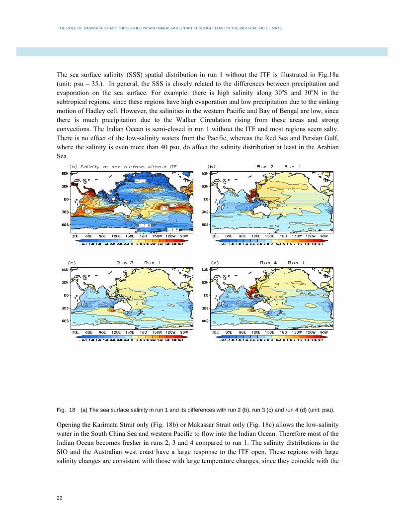
The sea surface salinity (SSS) spatial distribution in run 1 without the ITF is illustrated in Fig.18a (unit: psu – 35.). In general, the SSS is closely related to the differences between precipitation and evaporation on the sea surface. For example: there is high salinity along 30oS and 30oN in the subtropical regions, since these regions have high evaporation and low precipitation due to the sinking motion of Hadley cell. However, the salinities in the western Pacific and Bay of Bengal are low, since there is much precipitation due to the Walker Circulation rising from these areas and strong convections. The Indian Ocean is semi-closed in run 1 without the ITF and most regions seem salty. There is no effect of the low-salinity waters from the Pacific, whereas the Red Sea and Persian Gulf, where the salinity is even more than 40 psu, do affect the salinity distribution at least in the Arabian Sea.

Fig. 18 (a) The sea surface salinity in run 1 and its differences with run 2 (b), run 3 (c) and run 4 (d) (unit: psu).

Opening the Karimata Strait only (Fig. 18b) or Makassar Strait only (Fig. 18c) allows the low-salinity water in the South China Sea and western Pacific to flow into the Indian Ocean. Therefore most of the Indian Ocean becomes fresher in runs 2, 3 and 4 compared to run 1. The salinity distributions in the SIO and the Australian west coast have a large response to the ITF open. These regions with large salinity changes are consistent with those with large temperature changes, since they coincide with the


Page 23

locations with large changes of the Indian Ocean Circulation. Compared to run 1, run 2 reduces up to 1.2 psu in the Leeuwin Current region. The SSS reduction in run 2 becomes smaller westward along the SIO region. Runs 3 and 4 do not have such a gradient in salinity change in SIO. They also decrease the SSS with a maximum of 0.9 psu in this area. It should be noted that the SSS in the South China Sea (SCS) in runs 2 and 4 (Figs. 18b and d) is significantly increased to about 2.7 psu. This increase is possibly associated with a stronger SCST induced by the KSTF opening. The Pacific sea water, which is saltier than that in the SCS (Fig. 18a), passes through the Luzon Strait and moves into the SCS. The western Pacific Ocean is up to 0.6 psu saltier in run 2 and 0.3 psu saltier in run 4 than run 1. The spatial pattern in run 4 (Fig. 18d) is consistent with Song’s et al result (Song et al 2007), although the signs are opposite and they used the depth-averaged salinity between 0-50 m from a long-term run with a coupled atmosphere-ocean model. Figs.19 and 20 are the same as Fig. 18 but at 150 m and 350 m, respectively. When compared to run 1 at 150 m (Fig. 19a), the common features of the other runs include (Figs 19b, c and d): (1) the salinities are reduced in the SIO region and the eastern Pacific as with their SSS changes; (2) they are increased in the North Pacific, Arabian Sea and the southwest coast of Australia. Runs 3 and 4 have a litter larger salinity reduction in the SIO, Australian southwest coast and eastern Pacific, but gain a smaller salinity increase in the North Pacific than run 2. Run 3/4 decreases the salinity in the Australian southeast coast. It has reverse salinity changes along the east and west coasts of southern Australia like their variations in temperature fields. The reason is possibly that the Leeuwin Current is strengthened, but the EAC weakened when the MSTF is open. The salinity differences between run 2/4 with Java Sea opening and run 1 are much smaller at 150-m depth than the SSS in the SCS, since the Java Sea is very shallow, only around 50-m deep. The KSTF is hard to impact the deep SCS. The eastern Pacific at 150 m in runs 2, 3 and 4 becomes fresher than run 1 when the part/full ITF is open, since they produce a shallower thermocline.


24

Fig. 19 (a) The salinity at 150 m in run 1 and its differences with run 2 (b), run 3 (c) and run 4 (d) (unit: psu).

Fig. 20 (a) The salinity at 350 m in run 1 and its differences with run 2 (b), run 3 (c) and run 4 (d) (unit: psu).


Page 25

There is a different feature in the salinity changes at 350-m depth (Fig. 20) compared to the sea surface or 150-m depth when the ITF is open. Namely, the Indian Ocean becomes saltier at this depth. An anomalous high salinity extends westward from the west coast of Australia (Figs 20b, c and d); so does the anomalous warm temperature field (Fig.13). These temperature/salinity changes are possibly related to the anomalous westward current in the same area (Fig. 7). The SIO region is significantly affected by the ITF, so it is necessary to provide analyses for this region further. Fig. 21 displays the averaged salinity between 10oS-20oS in run 1 and its differences with the other runs. The salinity in the east in run 1 is about 0.6 psu larger than that in the west above 200 m (Fig. 21a). The deep ocean has a smaller salinity than the upper ocean. Besides the differences between run 1 and the other runs (Figs. 21b, c and d), there are some common features such as: the salinity become lower above 300 m, but higher below this depth. The maximum salinity increase occurs around 400 m. It is about 100-m deeper than the depth with the maximum temperature increase in the same region (Fig. 14). At the 400-m depth, run 3 has a little larger salinity increase than run 4, and both are 0.2 psu saltier than run 2. Run 2 seems to have a larger salinity reduction at the eastern upper ocean than runs 3 and 4, but a smaller reduction than them in the western upper ocean. It is possibly caused by a stronger SEC in runs 3 and 4 than run 1.

Fig. 21 (a) The averaged salinity between 10oS and 20oS in run 1 and its differences with run 2 (b), run 3 (c) and run 4 (d) (unit: psu).


26

The salinity for all experiments along 65oE and 90oE are illustrated in Figs. 22 and 23, respectively. They are the same with Figs 15 and 16 except for the salinity fields. The salinity is very high up to 37.7 psu in the Arabian Sea (Fig. 22a) but low in the Bay of Bengal (Fig. 23a). The fresher sea water from the western Pacific due to the part/full ITF opening impacts the salinity from south to north through the Indian Circulation (Figs 22/23b, c and d). It seems to superpose the salty deep water and depresses the pycnocline depth downwards. Like the large increase in temperature in runs 2, 3 and 4 along 65oE (Figs 15b, c and d) in comparison to run 1, the salinities in these runs are significantly saltier. No previous publications have been found to show the salinity sensitivity in the regions in response to the opening of the ITF. Run 2 has similar changes with runs 3 and 4 except a smaller salinity increase around 400 m in the SIO region. HG93 presented the salinity changes along 90oE with and without the ITF. Their result has a smaller reduction of salinity than ours result particularly between 10oS and 20oS, but almost no change occurs in the North Indian Ocean. The salinity change also shows reversal, but depth of reversal is below 600 m which is deeper than our results, about 300 m. It is possible that the model vertical resolution used in HG93 is coarser than ours.


Page 27

Fig. 22 (a) The salinity along 65oE in run 1 and its differences with run 2 (b), run 3 (c) and run 4 (d) (unit: psu).


28

Fig. 23 (a) The salinity along 90oE in run 1 and its differences with run 2 (b), run 3 (c) and run 4 (d) (unit: psu).


Page 29

Here we define the depth of maximum salinity in the subsurface as the halocline depth (Fig. 24). The halocline depth is deep in the Bay of Bengal and SCS, although the SSS is relative small due to a large precipitation in these regions. Another location with the deep halocline is in the SIO region, where there is a deep thermocline as well and a high SSS. Compared to run 1, the other runs have a significantly deeper halocline in the SIO region. They are similar to the changes in their thermocline depths, but the amplitudes in the halocline change seem is bigger.

Fig. 24 (a) The halocline depth in run 1 and its differences with run 2 (b), run 3 (c) and run 4 (d) (unit: m).


30

6. SUMMARY AND DISCUSSIONS

The ITF which is mainly forced by the horizontal pressure gradient connects the Pacific and Indian Ocean by its transport of mass and heat. Four experiments have been conducted here to examine how parts of ITF affect the Indo-pacific climate. Run 1 and run 4 are without and with the full ITF respectively. The KSTF or MSTF is only opened in run 2 and run 3. These runs 2 and 3 are actually natural extensions for the previous work, such as Hirst et al 1994; Lee et al 2005; Murtugudde et al. 1998; Song et al 2007; Santoso et al 2011 etc, which explore the role of ITF via closing or opening it completely. Although the MSTF whose annual mean meridional volume transport is 14.1 Sv southward in run 4 with the normal ITF is the main branch of the whole ITF system, the KSTF which has about 1.8 Sv southward transports in the same run has a non-trivial effect on the Indo-Pacific climate. The sea level in the western Pacific is about 100-cm high but only 20 cm high in the eastern Indian Ocean if the ITF is blocked completely (Fig.3a). Consequently, such large differences of sea level drive the warm and fresh sea water from the western Pacific to the Indian Ocean if the part/full ITF is open. Compared to run 1, the sea surface heights in the Pacific Ocean will reduce, but in the Indian Ocean they are increased almost everywhere, particularly in the South Indian Ocean. For instance, run 2 increases up to 20 cm (Fig.3b) and runs 3 and 4 even more than 30 cm (Figs 3c and 3d). The ITF in run 2, 3 and 4 produce an anomalous anti-cyclone transport in the South Indian Ocean including the Australian east coast (Fig.8) in comparison with run 1. However, this transport in run 2 seems much weaker than runs 3 and 4, since the KSTF transport is less than MSTF (Figs .4 and 5). The KSTF, MSTF and the whole ITF mainly enhance the South Indian Ocean Current, Agulhas Current, Agulhas Retroflection and Leeuwin Current, but weaken the East Australian Current. Nevertheless, the KSTF has a smaller effect on these currents than MSTF (Figs 6 and 7). The warm and fresh water originating from the western Pacific moves into the Indian Ocean via the ITF and leads to the substantial changes in the thermal structures in the Indian Ocean and equatorial Pacific. The depths of thermocline (Fig. 11) and halocline (Fig. 24) are depressed in the Indian Ocean, but uplifted along the equatorial Pacific. Consequently, a higher temperature in the Indian Ocean and a lower temperature in the equatorial Pacific occur (Figs 12-18). The largest change in temperature is located at about 100-500 m depth in the South Indian Ocean and 200-500 m depth in the Arabian Sea which has not been reported before. For example, along the 65oE section (Figs 15b-d), a temperature increase of more than 2oC is seen in run 2 and more than 4oC in runs 3 and 4 in relative to run 1 in the South Indian Ocean. The temperatures in the North Indian Ocean are even increased more. Run 2 gains more than a 3oC change, and runs 3 and 4 have more than a 5oC change. Note that the salinity has a large change as well in the same location in the North Indian Ocean (Fig. 22b, c and d). When the ITF is open, the Indian Ocean is generally fresher in the upper 200 m, but below 300 m depth the salinity becomes higher (Figs.17-23). The salinities averaged between 10oS-20oS at around 100 m in runs 2, 3 and 4 are reduced up to 0.7 psu compared to run 1, but at 400 m depth, they increase by 0.1 psu, 0.3 psu and 0.3 psu respectively. The low-salinity water masses from the western Pacific invade the Indian Ocean and dilute the original high salinity water. Meanwhile, the rise in sea


Page 31

level in the Indian Ocean makes the halocline depth sink. The deep oceans under the condition of ITF opening therefore become saltier. It should be noted that the SSS in the South China Sea has been substantially enhanced up to 2.7 psu in run 2 and run 4 when the KSTF is open (Figs 18b, d). It is possibly caused by the invasion of sea water through the Luzon Strait from the Pacific which is saltier than that in the SCS. Opening ITF will strengthen the upwelling in the eastern Pacific near the west coast of the South America, so the temperature becomes colder and the salinity is lower along the equatorial Pacific. In particular, the changes in thermal structure are pronounced at 150 m such as 2oC reduction in runs 3 and 4 and 1oC reduction in run 2 in the central Pacific (Figs 12, 19). Note that the east coast of South America even has a larger decrease in temperature and salinity than the other equatorial Pacific regions. Compared to run 1 without the ITF in the Indian Ocean climate, the differences from run 2 are generally smaller than those from run 3 or 4, since the volume transport of KSTF is smaller than that of MSTF (Figs 4 and 5), although the spatial patterns of these differences are similar. The results for both runs 3 and 4 are very close, since the MSTF accounts for 80% total ITF volume transport (Gordon 2005). However, the differences between runs 3 and 4 are different in different seasons. For example, their differences in boreal winter are larger than those in boreal summer (not shown). The annual mean meridional transport of KSTF is 1.8 Sv southward for the ITF open in run 4 but it increases to 3.3 Sv southward for the MSKF closed in run 2. The annual mean MSTF transport is 14.1 Sv in run 4 but it increases to 17.1 Sv if the MSTF is blocked in run 3. So runs 2 and 3 overestimate the normal transports of KSTF and MSTF compared with run 4, and slightly exaggerate the impact of KSTF and MSTF on the Indo-Pacific climate. Furthermore, runs 2 and 3 do not have the interaction between the KSTF and MSTF due to the closure of one of them. Although blockage of the part/full ITF creates an unrealistic oceanic state, it is still useful to understand its influence in controlling the mean and variability of the circulation and thermal structure in the Indo-Pacific. The climatological mean states have been investigated due to the part/full ITF opening in this study. In fact, the ITF is largely affected by the El Nino and La Nina events and thus has a strong interannual variability. How the different branches of ITF impact the Indo-Pacific climate variability and change should be further explored in future research.

ACKNOWLEDGEMENTS

This work is supported by the Australian Government Department of the Environment, the Bureau of Meteorology and CSIRO through the Australian Climate Change Science Program, and the NCI National Facility at the ANU.


32

REFERENCES

Antonov, J.I., Locarnini, R.A. Boyer, T.P. Mishonov, A.V. and Garcia, H.E. 2006: World Ocean Atlas 2005, Volume 2: Salinity. S. Levitus, Ed. NOAA Atlas NESDIS 62, U.S. Government Printing Office, Washington, D.C., 182 pp.

Bi, D. and Marsland, S.M. 2010: Australian Climate Ocean Model (AusCOM) Users Guide. CAWCR Technical Report No. 027, The Centre for Australian Weather and Climate Research, a partnership between CSIRO and the Bureau of Meteorology. 72 pp. ISBN: 978-1-921605-92-5. Bi, D., Marsland, S.J. Uotila, P. O’Farrell, S. Fiedler, R., Sullivan, A. Griffies, S.M. Zhou, X.. Hirst, A.C 2013: ACCESS-OM: the ocean and sea ice core of the ACCESS coupled model. Australian Met. Oceanogr. J., 63(1), 213-232. Gent, P., and J. McWilliams, 1990: Isopycnal mixing in ocean circulation models. J. Phys. Oceanogr., 20, 150–155. Gordon, A.L., 2001: Interocean exchange. Ocean Circulation and Climate, G. Siedler, J. Church, and J. Gould, Eds., Academic Press, 303–314. Gordon, A.L. 2005: Oceanography of the Indonesian seas and their throughflow, Oceanography, 18(4), 14– 27. Gordon, A.L., B.A. Huber, E.J. Metzger, R.D. Susanto, H.E. Hurlburt, and T.R. Adi 2012: South China Sea throughflow impact on the Indonesian throughflow, Geophys. Res. Lett., doi:10.1029/2012GL052021, in press. Griffies, S.M., 2009: Elements of MOM4p1: GFDL Ocean Group Tech. Rep. 6. NOAA/Geophysical Fluid Dynamics Laboratory, 444 pp. Griffies, S.M., and R.W. Hallberg, 2000: Biharmonic friction with a Smagorinsky-like viscosity for use in large-scale eddy-permitting ocean models. Mon. Wea. Rev., 128, 2935–2946. He, Z. M. Feng, D. Wang and D. Slawinski 2015: Contribution of the Karimata Strait transport to the Indonesian Throughflow as seen from a data assimilation model. Continental Shelf Research, 92, 16-22. Hirst, A.C., and J. S. Godfrey, 1993: The role of Indonesian Throughflow in a global ocean GCM. J. Phys. Oceanogr., 23, 1057–1086. Hunke, E C. and W.H. Lipscomb, 2008: CICE: The Los Alamos Sea Ice Model. Documentation and Software User's Manual. Version 4.0. T-3 Fluid Dynamics Group, Los Alamos National Laboratory, Tech. Rep. LA-CC-06-012.


Page 33

Jin, F-F., S.T. Kim, and L. Bejarano, 2006: A coupled stability index for ENSO. Geophys. Res. Lett., 33, L23708. doi:10.1029/2006GL027221. Johnson, G.C., B.S. Sloyan, W. S. Kessler, and K. E. McTaggart, 2002: Direct measurements of upper ocean currents and water properties across the tropical Pacific Ocean during the 1990s. Progress in Oceanography, Vol. 52, Pergamon, 31–61. Kajtar, J., A. Santoso, M. England, and W. Cai, 2014: Indo-Pacific Climate Interactions in the Absence of an Indonesian Throughflow. J. Climate. doi:10.1175/JCLI-D-14-00114.1, in press. Large, W.G., J.C. McWilliams, and S.C. Doney, 1994: Oceanic vertical mixing: A review and a model with a vertical K-profile boundary layer parameterization. Rev. Geophys., 32, 363–403. Large W.G. and S.G. Yeager 2009: The global climatology of an interannually varying air–sea flux data set. Clim Dyn, DOI 10.1007/s00382-008-0441-3. Tong, L., I. Fukumori, D. Menemenlis, Z. Xing and L. Fu, 2002: Effects of the Indonesian Throughflow on the Pacific and Indian Oceans. J. Phys. Oceanogr., 32, 1404–1429.

Locarnini, R.A., A.V. Mishonov, J.I. Antonov, T. P. Boyer and H. E. Garcia, 2006: World Ocean Atlas 2005, Volume 1: Temperature. S. Levitus, Ed. NOAA Atlas NESDIS 61, U.S. Government Printing Office, Washington, D.C., 182 pp.

Morel, A., and D. Antoine, 1994: Heating rate within the upper ocean in relation to its biooptical state. J. Phys. Oceanogr., 24, 1652–1665. Murtugudde, R., A.J. Busalacchi, and J. Beauchamp, 1998: Seasonal-to-interannual effects of the Indonesian throughflow on the tropical Indo-Pacific Basin. J. Geophys. Res., 103, 21425–21441. Murray, R.J., 1996: Explicit generation of orthogonal grids for ocean models. J. Comput. Phys., 126, 251–273. Qu, T., Y. Du, G. Meyers, A. Ishida, and D. Wang, 2005: Connecting the tropical Pacific with Indian Ocean through South China Sea, Geophys. Res. Lett., 32, L24609, doi:10.1029/2005GL024698. Rodgers, K.B., M.A. Cane, and N.H. Naik, 1999: The role of the Indonesian throughflow in equatorial Pacific thermocline ventilation. J. Geophys. Res., 104, 20551–20570. Santoso, A., W. Cai, M.H. England, S.J. Phipps, 2011: The Role of the Indonesian Throughflow on ENSO Dynamics in a Coupled Climate Model. J. Climate, 24, 585–601. Schiller, A., S.E. Wijffels, J. Sprintall, R. Molcard, and P.R. Oke, 2010: Pathways of intraseasonal variability in the Indonesian Throughflow region. Dyn. Atmos. Oceans, 50, 174–200, doi:10.1016/j.dynatmoce.2010.02.003.


34

Schneider, N., 1998: Indonesian Throughflow and the global climate system. J. Climate, 11, 676–689. Shinoda, Toshiaki, Weiqing Han, E. Joseph Metzger, Harley E. Hurlburt, 2012: Seasonal Variation of the Indonesian Throughflow in Makassar Strait. J. Phys. Oceanogr., 42, 1099–1123. Simmons, H.L., Jane, S.R., St. Laurent, L.C., Weaver, A.J., 2004: Tidally driven mixing in a numerical model of the ocean general circulation. Ocean Modell. 6, 245–263. Song, Q., G.A. Vecchi, A.J. Rosati, 2007: The Role of the Indonesian Throughflow in the Indo–Pacific Climate Variability in the GFDL Coupled Climate Model. J. Climate, 20, 2434–2451. Tozuka, T., T. Qu, and T. Yamagata, 2007: Dramatic impact of the South China Sea on the Indonesian Throughflow. Geophys. Res. Lett., 34, L12612, doi: 10.1029/2007GL030420. Tozuka, T., T. Qu, Y. Masumoto, and T. Yamagata, 2009: Impacts of the South China Sea throughflow on seasonal and interannual variations of the Indonesian throughflow. Dyn. Atmos. Oceans 47, 73–85.

Valcke, S. 2006: OASIS3 User Guide (prism_2-5). PRISM Support Initiative Report No 3, 64 pp.

Verschell, M., J. Kindle, and J. O'Brien, 1995: Effects of Indo–Pacific throughflow on the upper tropical Pacific and Indian Oceans. J. Geophys. Res., 100, 18409–18420. Wajsowicz, R.C., and E.K. Schneider, 2001: The Indonesian Throughflow’s effect on global climate determined from the COLA Coupled Climate System. J. Climate, 14, 3029–3042.

the role of karimata strait throughflow and makassar ... · the role of karimata strait throughflow...

Documents