1

Abstract

Data Envelopment Analysis (DEA) is an extensively studied, application driven doctrine foranalyzing Decision Making Units (DMUs) that consume inputs to produce outputs in adeterministic and quantifiable production process. The essence of DEA is captured in theminimum extrapolation principle, which guides us to envelope the data by the smallest setthat satisfies the imposed production assumptions. We thereby argue that the productionassumptions lie in the core of DEA, and the specification of assumptions is a determinantpractical consideration for all application of DEA. Unfortunately, this important matter is toooften confronted with persistent myths, illogical reasoning, or sheer ignorance.

In DEA, the production assumptions typically concern the shape of the production possibilityset in terms of such mathematical properties as monotonicity, convexity, and returns to scale.This dissertation discusses the meaning and the interpretation of these properties specificallywithin the DEA framework. Such aspects as economies of scale and of specialization as wellas incomplete or uncertain price information are considered. Our discussion focusesespecially on the various convexity properties, which are debated from both technologicaland economical perspectives. Moreover, some difficulties in the treatment of congestionusing the two-stage DEA techniques are pointed out. In addition to the theoretical discussion,we present some readily implementable operational DEA approaches which build moredirectly on the observed data.

Key Words: Data Envelopment Analysis (DEA), Non-parametric efficiency analysis,Production assumptions, Convexity, Free Disposable Hull (FDH), Economies of scale,Economies of specialization, Price uncertainty

2

3

THE ROLE OF PRODUCTIONASSUMPTIONS IN DATA

ENVELOPMENT ANALYSIS

Timo KuosmanenHelsinki School of Economics and Business Administration

Department of Economics and Management ScienceP.O. Box 1210, FIN-00101 Helsinki, FINLAND

TEL. +358 9 4313 8537FAX. +358 9 4313 8535

E-MAIL: kuosmane@hkkk.fihttp://www.hkkk.fi/methods/kuosmanen/

THIS DISSERTATION CONSISTS OF AN INTRODUCTORY SECTION AND THE FOLLOWING ARTICLES :

I. KUOSMANEN, T. (2001): DEA WITH EFFICIENCY CLASSIFICATION PRESERVINGCONDITIONAL CONVEXITY, EUROPEAN JOURNAL OF OPERATIONAL RESEARCH 132(2),83-99

II. CHERCHYE, L., T. KUOSMANEN, AND G.T. POST (2001): ALTERNATIVE TREATMENTSOF CONGESTION IN DEA: A REJOINDER TO COOPER, GU, AND LI, EUROPEAN JOURNALOF OPERATIONAL RESEARCH 133(1), 69-74

III. CHERCHYE, L., T. KUOSMANEN, AND G.T. POST (2000): WHAT IS THE ECONOMICMEANING OF FDH, A REPLY TO THRALL, JOURNAL OF PRODUCTIVITY ANALYSIS 13(3),259-263

IV. KUOSMANEN, T., AND G.T. POST (2001): MEASURING ECONOMIC EFFICIENCY WITHINCOMPLETE PRICE INFORMATION: WITH AN APPLICATION TO EUROPEANCOMMERCIAL BANKS, EUROPEAN JOURNAL OF OPERATIONAL RESEARCH, TO APPEAR

V. KUOSMANEN, T., AND G.T. POST (1999): NONPARAMETRIC EFFICIENCY ANALYSISUNDER UNCERTAINTY: A FIRST ORDER STOCHASTIC DOMINANCE APPROACH,HELSINKI SCHOOL OF ECONOMICS AND BUSINESS ADMINISTRATION, WORKING PAPERW-230

4

Preface

Now that I have typed the last corrections and refinements to this piece of work, it istime to look back and recall how this dissertation shaped into its present form. At the sametime, I have a pleasant opportunity to acknowledge those who have influenced this work andsupported my efforts through these years.

The initiative to this dissertation project came from Professor Pekka Korhonen andProfessor Jyrki Wallenius who recruited me as a full-time doctoral student to their MCDS -program at Helsinki School of Economics and Business Administration, the Department ofEconomics and Management Science in 1997. Ever since, Professor Korhonen, the chairmanon the department, has been a valuable advisor and supporter for me. As a successfulinternationally renowned scholar, he has been an excellent example for me to follow.Moreover, he has shown a lot of tolerance as my thesis supervisor, and has allowed me towork independently with my own ideas without putting me too much pressure. Another goodacademic role model for me has been Professor Jyrki Wallenius, the Vice Rector of ouruniversity. I wish to acknowledge with much appreciation the financial support from theGraduate School for Systems Analysis, Decision Making and Risk Management, which hasformed the primary source of funding for my dissertation project. Professor Seppo Salo, theformer head of our department, also earned my deep appreciation and respect. It isdevastatingly sad that he passed away before I had a chance to hand this completeddissertation to him.

Looking back, the excellent background knowledge from my underground studies atthe University of Joensuu Economics Department gave me an ideal starting point to thisdissertation project. Most notably, Dr. Tarmo Räty is guilty of introducing me to the topics ofthis thesis in the Econometrics classes on Spring-term 1996, and deepening my knowledgewhile advising my subsequent Master’s Thesis. Tarmo was preparing his own dissertation onthe topic at the time, and his genuine fascination of the topic gave the decisive inspiration forme to keep studying this literature. I believe the blueprints of this dissertation began to formalready in my undergraduate studies. I became fond of the nonparametric approach since Iwas fully aware of the difficulties in specifying an appropriate parametric function form forthe production function. Moreover, I had already developed healthy skepticism towards theconvexity postulate of DEA, which I found insufficiently motivated in most textbooks. (Inmy Master’s Thesis I already applied the non-convex FDH model.) Through these years, Ihave been in touch with Tarmo on a regular basis. Tarmo has proved a knowledgeablediscussant, a good friend, and a valuable source of older JPA papers, to which I am indebted.

In the beginning, the exact subject for my dissertation was not instantly clear, and ittook some while before it began to dawn on me. The key insight that eventually lead to thepublication of Article I below, and subsequently developed into this entire dissertation,occurred very suddenly and unexpectedly to me in a particularly creative moment during the5th European Workshop on Efficiency and Productivity Analysis held in Copenhagen onOctober 1997. I cannot explain how this happened, but the plan for this dissertation began tocrystallize, and I became very enthusiastic and motivated to start working.

I feel have been fortunate in many respects, but I should also stress that the luck issimply not enough. Refining even a most inspiring idea first to a journal article andsubsequently to a dissertation was a much more demanding process than I ever had expected.

5

Very soon I had to start revising my plans, as well as my papers. This appeared to go on andon, endlessly, over and over again. In this process I acquired dozens of nice ideas I was keenon presenting, but those ideas were scattered, unstructured, and seemingly unrelated.Unfortunately, none of those nice ideas seemed to please the referees enough to warrant apaper in any decent journal. Thinking of a complete book like this felt very remote, evenfrustrating at times.

Fortunately, I have had numerous opportunities to attend and present my work ininternational conferences, workshops and summer schools, thanks to the generous financialsupport from the Foundation of Helsinki School of Economic and Business Administration,the Foundation for Economic Education (Liikesivistysrahasto), Yrjö Jahnsson’s Foundation,and the Finnish Operations Research Society. The input from my 13 trips to 10 differentcountries on 4 different continents has been an essential factor. These professional meetingshave enabled me to adapt to the mindset of the field, keep up with the latest developments,make invaluable contacts with overseas colleagues, and get highly valuable feedback to myown studies, among other benefits. Especially the EURO Summer Institute at the Universityof Warwick on August 1998, and the Productivity Workshops since 1997 have had a greatimpact on my work. I wish to forward my deepest thanks all those wonderful scholars whohave shown interest in my work and have unselfishly shared their knowledge and insightswith me while down on the road. I am afraid the complete list would be too long to be printedhere, but I'm sure you know who you are!

These experiences helped me to realize that it was my most urgent task to learn towrite papers of publishable quality. At least for me, this was a process of trial and error.Consequently, I didn't give much though to the dissertation, but studied all interestingresearch problems I knew without following any systematic agenda. My strategy was to takethe advantage of the learning curve by producing a large number of papers and to spread therisk by investigating a wide variety of different problems and by targeting my papers todifferent journals. This was a time of very intensive work and rapid progress.

I have been privileged to share my efforts with two very ambitious, creative, clever,knowledgeable, work-oriented young scholars, Laurens Cherchye and Thierry Post, my non-convex brothers in arms. Indeed, teaming up with two highly productive co-authors hasgreatly enhanced my productivity. I have learned a lot from the intensive collaboration withLaurens and Thierry, and I hope the feeling is mutual. Perhaps most importantly, I learned tolove the writing process, even the associated critical examination, which felt quitediscouraging at first. Brainstorming sessions, anticipating the reactions of referees, andactually responding to the presented critique are actually very rewarding. And sharing this allwith good friends makes it even more fun. Cheers mates!

For roughly two years, I didn’t give much though to this project and felt a bit uneasyto even think about it. I could only hope that my hard work would eventually be rewarded bypapers that would form the dissertation some day. I took up the dissertation project againback to my drawing board on Spring 2000. Article I, the paper that took the greatest effort,had just been accepted for publication. Articles II and III had been accepted somewhatearlier. After the discouraging initial record of 8 rejections, I suddenly was in the happysituation where I had the required number of accepted publications at hand, and I merely hadto figure out a consistent story to bind the separate papers together. This was not the easiestpuzzle to solve, but I think I have managed to fit the pieces together surprisingly well.Looking back, I see that I've followed the correct strategy.

6

It is worth to mention here that I have done my best to preserve the five articles thatconstitute this dissertation as strictly as possible in their original form as intended forpublication, including any errors that I have become aware of afterwards. Hence, the articlesalso quite aptly reveal the development of my argumentation skills in the last years, fromArticle V which was written roughly two years ago in 1999 to the introduction that representmy present condition. I have revised some of our statements in the Introduction section whereI review these articles to highlight the contribution to the theme of this dissertation. Theerrors of more technical nature are addressed in Appendix 1.

I am grateful to my pre-examiners, Professor Rolf Färe and Professor Niels-ChristianPetersen, for their encouraging comments and constructive critique. Their fundamental workon the very topics of this dissertation has formed a source of inspiration for me through theseyears, and I think the influence of both these magnificent authors should be quite evidentfrom this thesis. To be honest, I could not name any more appropriate person to evaluate thecontribution of this dissertation than Professors Färe and Petersen. I consider it a great honorto have them both as the pre-examiners and the opponents of this dissertation.

Undoubtedly, the creative, internationally oriented, interdisciplinary atmosphere ofthe Quantitative Methods unit has also left its mark on my work. I have many pleasantmemories from the conference trips, summer schools and suchlike events with my colleaguesTarja Joro, Veli-Pekka Heikkinen, and Pirja Heiskanen. I would also like to thank MikkoSyrjänen, Heikki Siltanen, and Sari Rytökoski for lunch-hour discussions and bringing insome fresh new innovative sprit in the Methods group. My appreciation also goes to TuulaPaukkunen, the secretary of the unit, who has always kindly assisted me with thepracticalities.

I wish to acknowledge the inspiration from my parents Pertti and Eeva, whom I trulyrespect and admire. Since my parents did not have too good possibilities to study in theiryouth, I have always tried do my best and not to waste the excellent opportunities I have beenblessed with. My parents never put much pressure or high expectations on me, but have givenme the freedom to pursue my own routes. Their solid confidence in me has been a majorresource.

Last but not least, I am indebted to my wife Hanna who has managed our householdwith great care and skill, giving me the opportunity to focus my attention on this work. Myson Teemu deserves a special acknowledgement of the ability to cheer me up and bring meback down on the earth whenever needed. You are the greatest joy of my life. I realize thatmy long working hours, numerous overseas trips, and observing my intensive thoughtexperiments at home have often made you question is it really worth the effort. I am not sureyet, but I sincerely thank you for all the patience and love you have given me. As far as I candecide, my work is not completed yet, but this is just the beginning. Still, I hope thisdissertation proves my efforts have not been totally in vain.

Koivukylä, Vantaa, March 9, 2001.

Timo Kuosmanen

7

Contents

Abstract 1

Preface 4

Introduction 9References 22

Article I: DEA with Efficiency Classification Preserving Conditional Convexity 27

Abstract 271. Introduction 282. Static Taxonomy of Efficiency Measures 293. DEA Approach 314. Conditional Convexity 355. Efficiency Measurement 397. Concluding Remarks 45References 46

Article II: Alternative Treatments of Congestion in DEA: A Rejoinder to Cooper, Gu,and Li 51

1. Introduction 512. Definition of Congestion 523. Congestion Versus Structural Efficiency 534. Congestion Versus Free Disposability 555. Counterexamples 556. Conclusions 56References 57

Article III: What is the Economic Meaning of FDH? A Reply to Thrall 59

1. Introduction 592. Technical Efficiency Versus Profit Efficiency 603. Endogenous Prices and Price Uncertainty 604. The Interpretation of Substitution Rates 615. Conclusions 62Notes 62References 63

Article IV:Measuring Economic Efficiency with Incomplete Price Information: With anApplication to European Commercial Banks 65

Abstract 65

8

1. Introduction 652. Farrell Decomposition 673. Farrell Framework under Incomplete Price Information 704. Empirical Estimators 775. Empirical Illustration 806. Concluding Remarks 83References 84

Article V: Nonparametric Efficiency Analysis under Uncertainty: A First-OrderStochastic Dominance Approach 87

Abstract 871. Introduction 872. Efficiency Definitions 883. Efficiency Analysis under Uncertainty 904. Empirical Tests 975. Concluding Remarks 101References 102

Appendix 1: Errata 104

Appendix 2: Examples 107

9

Introduction

The notion ‘Data Envelopment Analysis ‘(DEA) was introduced by Charnes, Cooper,and Rhodes (1978). Today, DEA has become an extensively studied, application driven‘multipurpose tool’ for analyzing Decision Making Units (DMUs) that consume multipleinputs to produce multiple outputs,1 where the meaning of the words “DMU”, “input”, and“output” can be quite freely interpreted. We shall confine attention to production activitiesthat can be characterized as a deterministic process of transforming quantifiable andhomogenous inputs to quantifiable and homogenous outputs. That is, any stochasticvariations in the process as well as any quality differences and non-measurable factors areassumed non-existing, negligible for the purposes of the analysis, or ‘correctable’ by meansof some kind of data pre-processing. Although we do not impose any other qualifications onthe character of the potential activities or the numbers of inputs and outputs, thesepreconditions can still render some potentially interesting economic activities beyond thescope of our methods. For example, in the service sector the quality of ‘production’ is ofprimary importance, but it is extremely difficult - if not impossible - to measure the qualityaspect by the degree and accuracy required for efficiency analysis. Still, the focus on thequantifiable activities is the traditional stance of DEA, and we shall not deviate from it here.

DEA is studied and applied in a number of disciplines, including Economics andEconometrics, Operations Research and Management Science, Applied Mathematics, andStatistics. Most traditional application areas of DEA include such categories as agriculturalproduction, health care, education, financial institutions, and public sector production. More‘unusual’ applications of DEA include e.g. efficiency assessments with historical productiondata from Domesday England (McDonald, 1997), evaluation of alternative sites for the super-conducting super-collider in Texas (Thompson et al., 1986), and assessing the multi-dimensional performance of baseball players (Mazur, 1994)2. There exists a lot of evidencethat demonstrates the overwhelming popularity of DEA. See e.g. Seiford (1996) for a surveyarticle that lists over 600 published articles in refereed journals. We are not aware of thecurrent bibliometric statistics, but in our experience, the volume of DEA papers has recentlyincreased rather than declined.

As noted in the first paragraph of Article I, DEA has traditionally been used formeasuring various notions of technical and economic efficiency. However, in contrast toearlier accounts on DEA which typically present DEA as a synonym to efficiency analysis,we here de-emphasize the efficiency assessment aspects of DEA. On one hand, there alsoexist considerable alternative approaches to efficiency analysis, e.g. the parametric approachknown as Stochastic Frontier Analysis (SFA: see e.g. Bauer, 1990, for a survey). In fact, themost significant contributions to the actual efficiency gauges date way back to the ‘pre-DEA’era (e.g. Debreu, 1951; Shephard, 1951; Farrell, 1957) or have been presented at general levelwithout any direct association with DEA (e.g. Färe and Lovell, 1978; Zieschang, 1984;Chambers et al., 1998; among others). On the other hand, DEA is by no means limited to thecontext of efficiency analysis either. In fact, DEA is also employed for approximatingproduction functions, recovering unobserved shadow prices of inputs and outputs, providingbest-practice benchmarks, revealing shirking in principal-agent problems, and for decision 1 In the single-input single-output case, the original DEA model coincides with the traditional ratios of (partial)productivity indices, and the engineering definition of efficiency. In this sense, DEA could be viewed as anextension of the traditional output/input ratios to multi-variable settings.2 An application to the Finnish version of baseball, Pesäpallo, is reported in Kuosmanen (1999).

10

support in complicated choice situations, among other uses (see Article I, Section 1, forreferences).

By the above arguments, we see DEA essentially as a frontier estimation technique,which approximates the production frontier by a piece-wise linear envelopment supported bythe observed data points. In other words, DEA constructs a subset of the input-output spacethat contains all observed DMUs, i.e. DEA literally envelopes the data. In economicterminology, such an envelopment set can be viewed as an empirical approximation of theproduction possibility set characterizing the technology, i.e. the hypograph of the productionfunction. In general, our objective is to reveal some interesting information of the (unknown)underlying technology for the above-discussed purposes by studying the DEA frontiers.

Of course, one could easily imagine many alternative ways of enveloping any givendata. In DEA, the specification of the envelopment set is uniquely determined by theapparently universally accepted minimum extrapolation principle (Banker, Charnes, andCooper, 1984). According to this principle, the empirical DEA production set should be theminimal set that satisfies some imposed production assumptions.3 The productionassumptions of DEA conventionally include monotonicity (i.e. free disposability of inputsand outputs), convexity, and various notions of returns to scale (see e.g. Article I, Section 2,for formal definitions). Thinking in terms of the production frontier, monotonicity can beviewed as a first-order curvature condition, convexity can be seen as a second-order curvaturecondition, while returns to scale properties can be thought of as homogeneity conditions. Thisdissertation primarily focuses on the curvature conditions: monotonicity and convexity. Thereturns to scale properties will be devoted less attention, because 1) the treatment of returns toscale in DEA has already been thoroughly investigated in the earlier literature (see Article I,Section 2, for references), and 2) we are not aware of any acute problems in the standardtreatment at the moment.

From operational point of view, the minimum extrapolation principle connects DEA ina natural way to optimization. Indeed, DEA typically employs modern MathematicalProgramming, especially Linear Programming (LP) techniques. Much of the contemporaryresearch on DEA focuses on the operational issues of DEA. For example, how to formulate aLP problem in such a way that the constraints characterize a particular set of productionassumptions is a purely operational issue.

By contrast, some of the most profound methodological aspects of DEA apparentlyrest on a quite shallow foundation. For example, which assumptions to impose, and by whatcriteria, are issues which - to a large extent - determine the results one will obtain by DEA. Itis worth emphasizing that the specification of production assumptions is not merely atheoretical issue for academic debate. It is a question of vast practical importance for allapplication of DEA. It seems not exaggerated to claim the success or the failure of a DEAapplication essentially depends on its assumptions. Unfortunately, the DEA literature onlyoffers minimal guidance on the specification of the production assumption. Many valuable 3 By the term “production assumption” we explicitly refer to the maintained assumptions (axioms, postulates)concerning the properties of the underlying production set. Of course, we also need additional (explicit orimplicit) assumptions in DEA. For example, we earlier assumed that the production process does not involvestochastic variations and the data are error-free. Some authors have also imposed additional assumptions on thedistribution of inefficiency (see e.g. Banker, 1993). We here exclusively focus on the production assumptionsand the discussion on the role of the remaining premises falls beyond the scope of this dissertation. Interestedreaders can e.g. consult our recent working papers Kuosmanen and Post (1999) and Cherchye, Kuosmanen, andPost (2000, 2001a) for further discussions on the stochastic settings.

11

discussions with knowledgeable colleagues working in this field, as well as the feedback wehave received to our papers, give us an impression that quite many researchers andpractitioners feel puzzled about the production assumptions involved in DEA. We thereforebelieve the role of production assumptions forms a generally interesting as well aschallenging subject for this dissertation.

This dissertation consists of 5 distinct articles, which all contribute to the subject fromslightly different perspectives. We next take a brief outlook on these papers. Our purpose ismerely to clarify the connections between the independent papers, and to underline the mostinteresting implications to the main theme of this thesis. Moreover, we use this opportunity tobriefly discuss some additional points of interest that did not find their way to the originalpapers. All technical errors we have identified after completing the papers are addressed inAppendix 1.

Article I: Kuosmanen, T. (2001): ‘DEA with Efficiency Classification PreservingConditional Convexity’, European Journal of Operational Research 132(3), 83-99

The first article provides an elaborate introduction to the subject. First and foremost,this paper emphasizes that there is no valid justification for assuming production sets to begenerally monotonous or convex. For example, most commodities are more or lessindivisible, but indivisibility of inputs and/or outputs immediately violates both monotonicityand convexity. Furthermore, even if inputs and outputs were divisible, congestion ofproduction factors (Färe and Svensson, 1980) violates monotonicity, while economies ofscale and of specialization violate convexity. A classic reference to the economic significanceof non-convexities is Farrell (1959), who aptly summarized the economic importance of boththese qualifications:

“A glance at the world about us should be enough to convince us that most commodities areto some extent indivisible and that many have very large indivisibilities. Similarly, wheneverone refers to “economies of scale” and of “specialization”, one is pointing to concavities inproduction functions. There is thus no need to argue the importance of either indivisibilities orconcavities in production functions – the former are an obvious feature of the real world, andthe latter have constituted a central topic in economics since the time of Adam Smith.

(Farrell (1959), p. 378-379) 4

In his seminal 1957 paper, which laid the foundation for efficiency measurement ingeneral and DEA in particular, Farrell mostly focused on convex technologies in case ofconstant returns to scale. Nevertheless, Farrell also discussed the possibilities of economiesand diseconomies of scale, and he openly admitted the difficulties his method faces in case ofeconomies of scale.5 Interestingly, Farrell proposed to remedy this problem by the simple"grouping method", which means applying his method of enveloping data to subsets ofDMUs operating at the sufficiently similar scale size. Farrell and Fieldhouse (1962) furtherelaborated on this possibility. Moreover, Farrell and Fieldhouse proposed yet anotherapproach ("overall method") of applying the original Farrell method to data that is

4 A careful reader notes that (in standard terminology of mathematics) the hypograph of a concave productionfunction is a convex production set, and hence Farrell’s statement might appear somewhat confusing. However,Farrell deviated (for convenience) from the mathematical terminology and simply associated “departures fromconvexity” with “concavity”. (Farrell, 1959; footnote 3)5 Of course, diseconomies of scale are easily handled in the standard (VRS/BCC) framework. Perhaps thedifficulties Farrell saw with the treatment of the economies of scale might explain why Farrell never extendedhis method towards the so-called ‘variable returns to scale’ (VRS) technology.

12

transformed in such a way that constant returns to scale hold in the transformed input-outputvariables. These subsequent research efforts (following the seminal Farrell (1957) article)suggest that Farrell was genuinely concerned of the restrictive character of convexity in thepresent context.

The problem with economies of scale has received considerable attention in the morerecent DEA literature. Most notably, Petersen (1990) and Bogetoft (1996), and just recentlyBogetoft, Tama, and Tind (2000) and Post (2001b) have proposed DEA formulations thatrelax convexity of the production set, but maintain convexity of the input and/or outputcorrespondences. This specification allows for economies of scale, but (unfortunately)excludes potential economies of specialization in inputs and/or outputs. Indeed, should theinput and output correspondences always be convex, there would not be any incentive tospecialize in production of some particular inputs or outputs. The notion “economies ofspecialization” is by definition equivalent to non-convex input/output sets (e.g. Farrell, 1959;Arrow, Ng, and Yang, 1998). As noted already by Adam Smith in his famous needle factoryexample (to which Farrell refers in the quotation above), specialization can improveproductivity to a considerable extent. In Economic theory, increased specialization anddivision of labor are in fact widely regarded as the main sources of long-term economicgrowth. Moreover, in many areas of Economics, non-convexities in technology have beensystematically raised up as the driving force behind specialization (see e.g. Yang, 1994; Yangand Ng, 1993, 1995; Borland and Yang, 1995; Yang and Rice, 1994; Shi and Yang, 1995).

Petersen (1990) originally motivated the adherence to convexity in input and outputspace by referring to the ‘law of diminishing marginal rates of substitution’. This notion wasalso cited by Bogetoft, Bogetoft et al., and Post as the motivation of their DEA formulations.However, we cannot find other references to such law in the context of production in anyeconomic text we are aware of. The fact that neither Petersen nor the other authors citing thislaw presented any exact reference lead us to suspect an unintentional and unfortunateconfusion to the classic ‘law of diminishing returns’ (discussed in more detail in Article II).That law, however, has nothing to do with convexity of input or output correspondences.

In Article I we also put the content of this suspicious ‘law’ into question bydemonstrating that marginal rates of substitution cannot be guaranteed to diminish in case ofincreasing marginal products, i.e. the very situation for which these 'relaxed' DEA modelscited above were designed. Our example in Article I demonstrates how economies of scalecan actually give rise to economies of specialization under differentiability, even if the inputsor outputs would seem to be technical complements by their nature. To illustrate this pointmore specifically, consider the common textbook claim that input correspondences areconvex if production activities can be operated side by side without interfering with eachother (see e.g. the quotation of McFadden (1978) in Article I, p. 28). The following exampledemonstrates that this need not be true in case of economies of scale. Suppose the output ycan be produced in two independent production processes involving either input 1 or 2, i.e.

+ℜ∈21 , xx . Specifically, let the first production processes be characterized by theproduction function 2

1xy = , and let the second (alternative) process be 222xy = . Note that

both processes exhibit genuinely increasing returns to scale, with increasing marginalproductivity. Suppose further that we can operate these production processes side by sidewithout interfering with each other, so that the total amount of output is simply 2

221 2xxy += .

Interestingly, one can easily verify that the input correspondences associated with this

13

technology are non-convex for all y>0.6 This simple example suggests that when we allow foreconomies of scale, it is difficult to ascertain convexity of the input isoquants by reasoninghow inputs might interfere with each other. Rather, this example and the discussion inSection 3 of Article I demonstrate that economies of scale can lead to non-convex inputcorrespondences when there is no interaction whatsoever between the inputs, and even wheninputs are mutually complementary. By these somewhat discouraging findings we call forextra caution with postulating convexity properties a priori.

Besides drawing attention to some unrecognized problems with the standard DEAassumptions, Article I proposes a new less restrictive technology property so as to facilitate amore general (and hence ‘safer’) DEA approach. That approach is based on the novelconditional convexity concept introduced in Article I. The heuristics behind this notion arevery similar to that of the Farrell’s “grouping method”, i.e. we apply the standard DEA tosome subsets of DMUs for which convexity can be assumed to hold.7 The problem is, ofcourse, how to identify those subsets.

In Article I we confine special attention to the variant we call ‘efficiency preservingconditional convexity’, or shortly c-convexity. The starting point of that special case is theobservation that many important functions of DEA could actually be performed withoutimposing any production assumptions whatsoever, resorting only to the observed facts, i.e. tothe discrete set of observed DMUs. For example, we can classify which DMUs are clearlyinefficient –being dominated by at least one other DMU in each input and output- and whichDMUs seem efficient in the light of the given evidence. We refer to this efficiencyclassification obtained without any production assumptions whatsoever by spontaneousPareto-Koopmans efficiency classification. Of course, we can further identify seeminglyefficient DMUs as target points or benchmarks so as to facilitate learning from the ‘bestpractices’. In fact, the adjacent literature of nonparametric production analysis (Afriat, 1972;Varian, 1984) does resort to the discrete set of observed DMUs when testing for theconsistency of the observed production behavior with hypotheses of profit maximization orcost minimization. 8

Still, for other purposes of DEA it is desirable to go beyond the observations andconstruct a continuous empirical frontier. The heuristics behind the c-convexity property arethe following: Analogous to the standard DEA, we interpolate the data by constructing apiece-wise linear frontier consisting of hyperplane segments, where the empirically efficientDMUs constitute the vertices of the frontier. We deviate from the basic DEA in that we donot allow any arbitrary ad hoc assumptions to violate the natural spontaneous Pareto-Koopmans efficiency classification. This implies that the resulting production set can be non-convex. We show that in theory, conditional convexity (and hence c-convexity as its specialcase) implies both monotonicity and convexity, but not conversely. Therefore, conditionalconvexity is a more general technology property than either convexity or monotonicity. 6 The input sets are convex if the Hessian matrix of the production function is negative semidefinite. However,the Hessian matrix associated with this technology is a diagonal matrix (since 012

221

2 =∂∂∂=∂∂∂ xxyxxy ), thediagonal consisting of positive numbers ( 22

12 =∂∂ xy and 42

22 =∂∂ xy ). Hence this matrix is positive definite,

implying concave input isoquants and non-convex input sets.7 Interestingly, the modern equivalent of the Farrell and Fieldhouse “overall method” is the “TransconcaveDEA” approach studied by Post (2000a,b). Of course, the main difficulty with that approach is the specificationof appropriate transformations. Post has investigated this problem in more detail, and has obtained quitepromising results in simulated experiments by using empirical specification tests.8 Most notably, Banker and Maindiratta (1988) and Färe and Grosskopf (1995) have stressed the kinshipbetween the distinct traditions of nonparametric production analysis and DEA.

14

As discussed in Article I, a potential problem of the proposed approach is thecomputational complexity. While the basic DEA models involve solving a single LP problemfor each DMU we desire to evaluate, the c-convex DEA model presented in Article I boilsdown to disjunctive programming. Article I illustrated how one could characterize thereference peer groups, and subsequently compute efficiency measures by solving a finittesequence of LP problems. Unfortunately, the total number of LP problems one needs to solvein this primitive algorithm can be very large depending on the data set. It is therefore ofconsiderable interest to note here the encouraging result that more efficient computationalprocedures do exist. Very recently, we have found a way of reformulating the disjunctiveprogramming problem associated with the c-convex DEA model equivalently as a binary (0-1) Mixed-Integer Linear Programming Problem (MILP).9 Attractively, computing efficiencymeasures relative to the c-convex technologies can be effectively conducted by solving asingle MILP problem per each DMU to be evaluated. Today, highly efficient algorithms forsolving MILP problems are generally available, and hence (in sharp contrast to theconclusions of Article I) we no longer need to worry about the computational burden of the c-convex DEA model.

From statistical point of view, we can think of the input-output data of DMUs as asample drawn from the production set, and DEA efficiency measures as estimates for the trueefficiency measure. Banker (1993) first demonstrated that these DEA estimates are consistentunder some relatively general distribution assumptions (see Simar and Wilson, 2000, for anup-to-date discussion). In Article I we express the conjecture that under the standarddistribution assumptions considered by Simar and Wilson (2000), a DEA model based on c-convexity should be statistically consistent for a more general class of technologies than thestandard DEA (and Free Disposable Hull (FDH: Deprins, Simar, and Tulkens, 1984)) modelsthat build on the conventional monotonicity and/or convexity properties.

In finite samples, DEA efficiency estimator that builds on c-convexity is exposed tosampling error like all DEA estimators. In Article I we have focused on a variant of c-convexity that preserves efficiency classification of each observed DMU, but not theclassifications of the unobserved production vectors. Consequently, in contrast to thestandard DEA models, adherence to the minimum extrapolation principle does not suffice toguarantee that the empirical production set is contained within the underlying productionset.10 In other words, inefficiency of some DMUs could be exaggerated in a small sample.Still, in larger samples, under the standard assumptions on the data generating process, the c-convex DEA efficiency estimates should converge for a more general class of technologiesthan efficiency estimates of any earlier DEA model. Moreover, the c-convex DEA model cannever yield smaller efficiency estimates than the convex DEA models. Hence, in light of thealternatives, it would seem hypocritical to immediately object the potential negative smallsample errors associated with the c-convex DEA efficiency estimates. Specifically, if the c-convex DEA efficiency estimates happen to exaggerate inefficiency, the convex DEAalternative will always do even worse because of its inherent specification error. 9 The MILP formulation is presented in the paper in the forthcoming working paper Kuosmanen (2001), whichis available from the author upon request. Since the contents of the dissertation have already been formallyexamined and approved, we refrain from drastic revisions at this stage, following the advise of the honorablecustos.10 One might attribute this result to the shortcomings of the conditional convexity property. Conversely, thisresult can be viewed as a rather serious limitation of the fundamental minimum extrapolation principle, i.e.adherence to this principle implies containment of the empirical production set within the true production setonly under some particular production assumptions, but not necessarily in general.

15

Finally, it is always possible to apply the c-convexity condition, in addition to theobserved DMUs, to all imaginable input-output vectors as well. It would be straightforwardto demonstrate that this second variant of c-convex DEA would simply give the intersectionof MH(S) and CH(S), where MH(S) is the monotone hull of observed DMUs and CH(S) is theconvex hull of observed DMUs (using the notation and terminology of Article I). This setwould of course be contained within the underlying production set for all technologies thatsatisfy the c-convexity property. But unfortunately, by this more conservative approach welose the attractive ‘smooth’ frontier associated with the first variant, and the efficiencymeasures no longer are continuous and subdifferentiable. There are no free lunches.Nevertheless, this second variant could prove an interesting route to accommodate‘congestion’ in the Free Disposable Hull (FDH) framework. That issue that has attractedsome interest among dedicated researchers (see e.g. Kerstens and Vanden Eeckout, 1999).The final remark smoothly moves us to Article II.

Article II: Cherchye, L., T. Kuosmanen, and G.T. Post (2001): ‘AlternativeTreatments of Congestion in DEA: A Rejoinder to Cooper, Gu, and Li’, EuropeanJournal of Operational Research 133(1), 69-74

This paper grew out from two referee reports to the article by Cooper, Gu, and Li(2001), who advocated use of their new approach to deal with congestion in DEA bypresenting some numerical counterexamples against the established Färe, Grosskopf, andLovell (FGL: 1983, 1985) approach. Since many distinguished authors of the field apparentlyhave faced difficulties with the somewhat confusing terminology, we first discussed themeaning and the relationships of the notions of congestion, free disposability, and structuralefficiency. By this clarification we hope to direct the on-going debate on this subject towardsmore substantial issues.

We next refuted the claims of Cooper et al. by modifying their counterexamples.Specifically, we imposed some standard technology properties (explicitly assumed by FGL)to demonstrate that the alternative approach advocated by Cooper et al. can ‘fail’ in exactlythe same way the FGL model was claimed to fail. To enable readers to follow the counter-arguments, we have placed some necessary information on the examples available inAppendix 2.

But in addition to the obvious, we tried to use this opportunity to emphasize twopoints of far greater importance in the present context. Firstly, we expressed our skepticismfor empirical identification of congestion in a finite sample by any two-stage DEA model(including the two specific models subject to this debate). Our concern essentially arises fromthe fact that we typically only observe a sample of feasible input-output combinations, ratherthan the full (super)population. If we observe a particular input-output combination, webelieve it must be feasible. But if we do not observe a particular input-output vector, it doesnot yet imply this production plan would be infeasible. Unfortunately, the two-stage DEAapproaches do not take into account the possibility that some feasible production plans maynot be observed. In Article II we refer to this phenomenon by the statistical term ‘samplingerror’. The problem is, the proposed congestion indicators can reflect violations ofdisposability as they are expected to do, but they can equally well reflect occurrences whereour finite sample of DMUs simply does not include observations from all regions of theefficient frontier. Unfortunately, we cannot immediately distinguish the former desirable

16

effect from the latter unwanted influence by these techniques.11 We therefore suggestedestablishing a stronger connection with the rapidly developing DEA literature that explicitlydeals with the issue of sampling error (e.g. Simar and Wilson, 2000).

Secondly, we politely called for more rigor and transparency with the assumptions. Inthis respect, the treatment by Cooper et al. is an example that falls below any standards.Firstly, Cooper et al. ignored the production assumptions on which the FGL approach wasbuilt on – the assumptions that FGL had quite clearly stated in their texts. Worse still, Cooperet al. did not mention what kind of assumptions their own method would necessitate. Yet,these authors made the claim that their own approach is more meaningful than the FGLalternative.

Looking at the bigger picture, these recent discussions are directly related to the olddebate between the advocators of the ‘loose paradigm’ (which Cooper et al. (2000) call the“application oriented” approach) and the more rigorous ‘axiomatic approach’ to DEA(represented most notably by Färe and Grosskopf). The present discussion has aptly revealedthe key advantages of the axiomatic approach. Our firm conviction is that when one becomesconcerned of the meaning of the numbers generated by sophisticated DEA formulations (likeCooper et al. did), it is impossible to present any sensible argumentation if the maintainedpremises remain concealed. Yet, we would stress that the axioms are merely usefulinstruments for the logical reasoning. As Article III next aptly demonstrates, it is possible toreason logically even without mechanically resorting to axiomatics. The ultimate limitation ofany axiomatic system is that the axioms themselves cannot be proved correct by the system’sinternal logic, but must be justified by external arguments.12 This leaves room for a moreholistic reasoning (see Conclusions below for further discussion), which has been absent inthe contemporary DEA literature.

Article III: Cherchye, L., T. Kuosmanen, and G.T. Post (2000): ‘What is theEconomic Meaning of FDH? A Reply to Thrall’, Journal of Productivity Analysis13(3), 259-263

Article III continues along the lines of the previous paper, but returns back to theconvexity property, now from the perspective of economic efficiency. This paper was writtenas a response to Thrall (1999) who claimed that the non-convex FDH efficiency analysis hasno economic meaning whatsoever. Thrall based his argument on his principal theorem, whichessentially demonstrated that a DMU diagnosed technically efficient in the FDH model canbe highly inefficient in terms of profit maximization at exogeneously given and fully certainprices.

In our opinion this result is not surprising at all, and certainly does not give rise to thestrong negative conclusions drawn by Thrall. Most importantly, a similar result can be easilydemonstrated to hold for the standard convex DEA models as well, i.e. a technically efficientDMU according to a DEA model can equally well be highly inefficient in terms of profit 11 Actually, a similar identification problem pertains to the identification and measurement of scale inefficiencyby analogous two-stage DEA approaches. For example, we might be tempted to explain observed productivitydifferences by technical and scale inefficiencies. Unfortunately, DEA based finite sample inference may beseriously biased because the sampling error can only increase the technical efficiency component while it tendsto systematically decrease the scale efficiency component (essentially because the CRS technology is lessvulnerable to the sampling error). That is, we expect the two-stage DEA approach to exaggerate the importanceof scale efficiency relative to technical efficiency.12 This point is manifested in the Gödel’s famous impossibility theorem.

17

maximization. This is because technical efficiency is a necessary, but not sufficient conditionfor economic efficiency. Unlike Thrall, we do not interpret that as a failure of DEA.

Interestingly, when we take the prices explicitly into account to measure profitefficiency instead of technical efficiency, the convexity assumption becomes redundant. Thatis, profit efficiency measured relative to the convex monotone hull of DMUs always equalsprofit efficiency relative to the monotone hull (=FDH) of observations, which in turn equalsprofit efficiency relative to the discrete set of observed DMUs. This last observation followsdirectly from the fundamental theorems of nonparametric production analysis by Afriat(1972) and Varian (1984). Therefore, FDH is an equally meaningful technologyapproximation as the convex DEA (VRS) model in the economic circumstances consideredby Thrall. These arguments ipso facto refute the claim of Thrall. But again, we used theopportunity to take this line of reasoning a little bit further.

We argue that in many empirically relevant situations, the DMUs do not take prices asexogenously given and fully certain. If we consider profit-maximizing behavior underendogenous prices or price uncertainty, however, the redundancy result of convexity ceasesto hold in general. We illustrate the endogeneity argument by a simple numerical exampleadopted from Thrall.13 That example demonstrates that under imperfect competition whereprices generally depend on the supplied/demanded quantities, a DMU can maximize profit,but still become classified as inefficient in a convex DEA model. As for the price uncertainty,we refer to Article V included in this thesis. The discussion of Article III hence provides anillustrative verbal introduction to the perspective of economic efficiency investigated in thelast two papers.14

Article IV: Kuosmanen, T., and G.T. Post (2001): ‘Measuring Economic Efficiencywith Incomplete Price Information’, European Journal of Operational Research, toappear.

Article IV first rephrases the foundations of the economic efficiency measurement. Inthis perspective, we motivate the Farrell technical efficiency measure merely as a ‘proxy’ foreconomic efficiency. Interestingly, economic efficiency notions require very detailed price(or cost) information, while the technical efficiency proxy cannot immediately utilize anyprice information whatsoever. In our experience, however, most research situations arecharacterized as the intermediate cases where some important price data are unavailable orpoorly measured, but still, some bounds on the relative magnitudes of prices can be presentedbased on theoretical knowledge or practical experience of the application area. Hence, in thispaper we investigate the possibility of improving the Farrell’s proxy by utilizing all priceinformation at hand. For sake of generality (and convenience), we assume the price domaintakes a form of a convex pointed cone, which allows for a gradual transition from the perfectprice information to the opposite case of no price information. We show how one can derivean interval estimate for cost efficiency by applying the Farrell input measure to ‘convexified’input correspondences which are augmented by the polar cones associated with the pricedomain.

13 It is worth to add that (like Thrall) we did not impose any production assumptions, but studied meaningfulnessof monotonicity from the point of view of the economic objectives.14 For further discussion on price endogeneity and uncertainty, we refer to our recent working paper Cherchye etal. (2001b).

18

From operational point of view, these interval estimates can be convenientlycomputed using the standard weight-restriction, assurance region, and cone-ratio techniques,which have been extensively studied in the recent DEA literature (see Article IV forreferences). In fact, the incorporation of price information to DEA is frequently mentioned asthe motivation of using these techniques. However, the interpretation of the resulting‘efficiency scores’ appears to be an acute problem of those techniques, which seems to causea lot of confusion among the practitioners. Hence, we saw it worth to elaborate on theeconomic foundation by this paper.

In addition to this theoretical elaboration, our treatment also suggests some distinctmaterial advances in comparison to the earlier proposals. Firstly, we proposed to consider theentire interval of outcomes instead of solely focusing on the ‘optimistic’ upper bound. Thisgives a more complete picture of the magnitude of the economic losses due to inefficiency onone hand, and the gains obtainable by improving the performance on the other.15 Secondly,we stressed that not all price information is always desirable – a point that is typically ignoredin the weight-restriction literature. In essence, the value of the additional price informationdepends on the notion of economic efficiency that is seen appropriate for the situation athand. For example, if we are primarily interested of cost efficiency, the output prices arecompletely useless. Thirdly, we again emphasized the restrictive nature of productionassumptions, especially convexity. Thus far, the weight restriction approaches have beenpredominantly employed in the convex DEA framework.16 For example, one can motivateconvex input sets by the focus on cost efficiency, but that is not a valid excuse for assumingconvex output sets. Consequently, we showed how to incorporate additional priceinformation in the less restrictive FDH technology. Interestingly, the cost efficiency estimatescan in this case be computed by the standard LP codes, complemented with a very simpleenumerative principle. An application to European commercial banks demonstrates that evensome slight restrictions on the feasible price domain can result in substantial improvement inthe efficiency estimates (provided that the restrictions are correct).

Article V: Kuosmanen, T., and G.T. Post (1999): ‘Nonparametric Efficiency Analysisunder Uncertainty: A First-Order Stochastic Dominance Approach’ Helsinki School ofEconomics and Business Administration, Working paper W-230

Finally, in Article V we extend the economic efficiency analysis circumstancescharacterized by price uncertainty. More often than not, the producers must committhemselves to certain production plans before they have completely certain information onthe input or output prices – consider capital inputs for example. Therefore, the ex postperformance evaluation undertaken with DEA may not be appropriate when producers faceex ante price uncertainty. Of course, evaluation of ex ante efficiency of production plans is acomplicated task, and to the best of our knowledge, this paper is the first serious attempt toshift the perspective of DEA towards this direction.

To take the risk preferences of DMUs explicitly into account, we formulated theproduction objective to be maximization of the expected utility of profit. Interestingly, we

15 Unfortunately, there is an annoying technical error associated with the lower bound, which may cause someconfusion. The error is corrected in the Appendix.16 For example, Seiford (1996) explicitly stressed that the weight restriction techniques are available for theconvex DEA models, which can give an impression that weight restrictions cannot be incorporated into the FDHframework. As far as we know, Article IV makes the first proposal to introduce the weight restrictions to theFDH analysis.

19

have later discovered that this objective function has established as the standard in the theoryof firm under uncertainty (the classic references are McCall, 1967; and Sandmo, 1971). Still,it should be emphasized that the nonparametric efficiency tests proposed in this paper do notessentially depend on the expected utility hypothesis. In contrast to our statement on p. 91(Section 3, the last paragraph), a wide range of alternative non-expected utility theories areconsistent with the First-order Stochastic Dominance (FSD) criterion, and can hence beimmediately accommodated within our framework.

Our objective is to assess whether the evaluated input-output vector could be viewedas a rational ex ante choice that complies with some unknown well-behaved decision rule (i.e.is consistent with the FSD criterion) under some unknown price distribution. Using a similarstructure of the price domain as in Article IV, we derive the necessary and sufficientconditions for a DMU to be consistent with the FSD condition. Interestingly, we note thatthese conditions include some standard conditions of economic and technical efficiency asthe limiting special cases. This indicates the possibility to extend the traditional ex postefficiency conditions in a relatively straightforward way towards ex ante efficiencyevaluation. Moreover, this proves that the proposed FSD test approach is easilyimplementable by the standard computational techniques.

Of course, we might also think of a degree measure of inefficiency in case our testindicates inefficiencies. However, such measure should almost inevitably be based on the‘utility’ scale. But unfortunately, measuring the utility loss of inefficiency seems highlyproblematic, given our nonparametric orientation. Moreover, the complexity of the currentsetting involving price uncertainty appears to render the dual approach of Debreu (1951)ineffective. Due to these difficulties, we abstract from measuring the degree of inefficiencyand merely focus on identification of inefficient DMUs.

As for the production assumptions, we elaborate on our earlier argument (see ArticleIII) that under price uncertainty the convexity of production possibility set is generally not aharmless condition, which is in a sharp contrast to the standard result under price certainty. Incontrast to convexity, we show that monotonicity does remain as a harmless condition in thenew setting as far as the utility function is increasing in profit.

The restrictive nature of convexity essentially arises from the allowance for riskpreferences, i.e. risk aversion. Interestingly, it can be easily demonstrated that if producersare assumed to be risk neutral, the standard result of harmless convexity is restored. This isbecause risk neutrality implies that the expected utility of profit always equals the utility ofthe expected profit, or equivalently, the utility of profit at the expected prices, i.e. (using theobvious notation)

EU(π) = U(Eπ) = U(E(p)y - E(w)x).

To prove the harmless character of convexity in this case, one can simply rephrase theAfriat’s Theorem (e.g. Varian (1984)) in terms of expected prices (instead of the fully certainprices).

It remains an interesting challenge for future research to investigate how the power ofthe proposed nonparametric stochastic dominance test could be improved by imposing higherorder restrictions on the risk preferences, e.g. by using the Arrow-Pratt measure of riskaversion or the certainty equivalent as instruments. Conversely, it would be interesting to find

20

a way to recover how large the degree of risk aversion or the certainty equivalent would haveto be in order to be able to ‘rationalize’ a given non-dominated input-output vector.

Conclusions and Discussion

We have argued that DEA is essentially a nonparametric approach to frontierestimation, in which the imposed production assumptions play a central and determinant role.We discussed the meaning and the interpretation of the production assumption, whichtypically include such properties as monotonicity, convexity, and returns to scale. Weintroduced some new aspects such as economies of scale and of specialization as well asincomplete or uncertain price information into this discussion. Our remarks especiallyfocused on the various convexity properties, which were debated from both technological andeconomical perspectives. Moreover, some difficulties in the treatment of congestion using thetwo-stage DEA techniques were pointed out. In addition to the theoretical discussion, wepresent some readily implementable operational DEA techniques, most notably the c-convexand the price-augmented production sets, which build directly on the observed data.

Although the mathematical definition of production assumptions does not leave anyroom for speculation, there are considerable differences in the interpretation of theassumptions between different authors. We therefore find it illustrative to categorizealternative perspectives to production assumptions according to their source and theirfunction. The production assumptions can originate from 1) rational arguments and intuitionor 2) empirical considerations and evidence. Secondly, we can categorize the productionassumptions according to their intended purpose as i) descriptive statements or ii)instrumental hypotheses. This classification gives us four alternative views of the nature ofproduction assumptions.

Table 1: Alternative perspectives to production assumptions: examplearguments and representative references

Rational EmpiricalDescriptive Production possibilities are

convex, because themanufacturing process is bothadditive and divisible.

Arrow and Hahn (1971)

Evidence from empiricalstudies supports theassumption that productionpossibilities are convex.

Tulkens (1993)Instrumental Convexity is a 'harmless'

regularity condition underprofit maximization.

Varian (1984)

"Decision-Makers find theresults of the convex DEAmodel more convincing thanthe results from the non-convex model."

Table 1 illustrates these four different perspectives in case of the convexityassumption. To illustrate each category, we formulated some arbitrarily chosen examplearguments to justify the convexity assumption. Moreover, we included a representativereferences to papers where the perspective is present. Note that our examples and thereferences are not meant to be directly related. For example, Tulkens (1993) takes exactly theopposite stance to the example argument presented in Table 1. Moreover, we are not aware of

21

any explicit arguments where empirical evidence had been used to back up instrumentalassumptions, and we see that this position is virtually non-existing in the literature.

In the articles that constitute the main content of this dissertation, we have criticizedproduction assumptions from all these perspectives, focusing on various convexityassumptions. Firstly, we have presented rational arguments for why standard productionassumptions like convexity need not hold in reality, drawing attention to such aspects aseconomies of scale and of specialization. Moreover, we have pointed out some importantlimitations in the line of reasoning presented in the earlier literature. We refer especially toArticle I for further discussion.

Secondly, we have investigated the existing empirical evidence, which cannot bedescribed exhausting at the moment, and found some indication of violations of the commonassumptions (see e.g. Article I, Section 3, p. 33). However, we consider the existing empiricalfindings regarding the production properties tentative at best. In our opinion, a seriousempirical program would necessitate more developed statistical techniques, which couldaccount for both the sampling error and the data problems. Although some considerable stepshave recently been taken in that research direction (see e.g. Article II, Section 6, forreferences), a number of problems remain unsolved. Furthermore, we face rather fundamentalidentification problems whenever we investigate a spontaneously generated real-worldeconomic data (rather than fully controlled and isolated production experiments, like e.g.field trials in agriculture). For example, the fact that we do not currently observe any DMUproducing in the congested or non-convex region of the production frontier does notgenerally imply the production technology would be monotonous and convex. It may simplybe the case that the economic motives (e.g. profit maximization) drive the DMUs to produceat the economically advantageous regions of the frontier even though the underlyingtechnology actually is non-monotonous and non-convex. That is, an economic selectioneffect occurs, which makes the data look like it had come from a "nicely behaved" convexmonotonous technology (analogous to e.g. Afriat, 1972; and Varian, 1984). Thisidentification problem is an important (yet largely ignored) consideration in many functionsof DEA, including the planning of the future activities, in the (re)allocation of resources tothe DMUs, as well as in the forecasting of the firm behavior.

Thirdly, from the purely instrumentalist perspective, we do not see there any materialvalue whatsoever in such production assumptions that are harmless, i.e. do not interfere withthe results. As discussed in Article III, the discrete set of observations would then give theidentical results. That is, we object using the duality relationships between the economicobjective functions and the technology representations as a justification for productionassumptions in DEA. On the other hand, the instrumental statistical argument of imposingproduction assumptions to reduce the sampling error in efficiency estimates has the obviouscost of increased risk of specification error, without any associated gain in the asymptoticproperties. As noted above, we are not aware of systematic instrumentalist accounts based onempirical findings.

By the above arguments, we call for displacing the production assumptions from theleading role they now play the contemporary methodology. Instead, we would like to seethere a genuinely data driven DEA, which truly lets the data 'speak for itself' rather than forceit to the idiom of some arbitrary ad hoc postulates. In our opinion, the first important step inthe correct direction is taking the discrete set of empirical observations as the basic startingpoint of investigations. Note that focusing on the discrete set of observations is perfectly in

22

line with the minimal extrapolation principle of DEA when no production assumptions areenforced. The five articles below all share this data focused perspective. It is evident fromthese papers that our point is not to abandon envelopment sets or DEA. We have merelyobserved that the strongest cases for enveloping the data are typically the motivated from theperspective of economic conditions, objectives or efficiency criteria, rather than formtechnology properties. Under such circumstances, the discrete set of observations is at leastan equally good technology representation as any envelopment set. We do recognize thepossibility of eliciting technical information (e.g. engineering consideration, see e.g. Chenery,1949) that can be incorporated into the analysis by means of global or local productionassumptions. However, we find this a quite difficult route, limited to very simple productionactivities.

Finally, we think the fully blown methodology would also more explicitly recognizethe serious data limitations, incomplete information, and uncertainties involved in production.This would call for more transparent model specification and justification of themethodological choices, reflected also in the conclusions and implications. Most certainly,this means 'weaker' results in the sense that greater emphasis should be based on investigationof alternative scenarios, speculative 'what if…' thought experiments, examination of theextreme cases, and more systematic sensitivity and robustness analyses. However, results ofsuch comprehensive analyses would almost certainly be 'stronger' in terms of their empiricalcontent.

REFERENCES

Afriat, S. (1972): Efficiency Estimation of Production Functions, International EconomicReview 13(3), 568-598

Arrow, K.J., and F.H. Hahn (1971): General Competitive Analysis, Holden-Day Inc., SanFrancisco. Oliver & Boyd, Edinburgh.

Arrow, K.J., Y.-K. Ng, and X. Yang (Eds.) (1998): Increasing Returns and EconomicAnalysis, New York: St. Martin's Press; London: Macmillan Press

Banker, R.D. (1993): Maximum Likelihood, Consistency and Data Envelopment Analysis: AStatistical Foundation, Management Science 39(10), 1265 – 1273

Banker, R.D., A. Charnes, W. W. Cooper (1984): Some Models for Estimating Technical andScale Inefficiencies in Data Envelopment Analysis, Management Science, 30(9), 1078 – 1092

Banker, R.D., and A. Maindiratta (1988): Nonparametric Analysis of Technical andAllocative Efficiencies in Production, Econometrica 56(6), 1315-1332.

Bauer, P.W. (1990): Recent Developments in the Econometric Estimation of Frontiers,Journal of Econometrics 46(1/2), 39-56

Bogetoft, P. (1996): DEA on A Relaxed Convexity Assumption, Management Science 42(3),457-465

23

Bogetoft, P., J.M. Tama, and J. Tind (2000): Convex Input and Output Projections ofNonconvex Production Possibility Sets, Management Science 46(6), 858-869

Borland, J., and X. Yang (1995): Specialization, Product Development, Evolution of theInstitution of the Firm, and Economic Growth, Journal of Evolutionary Economics 5(1), 19-42

Chambers, R. G., Y. Chung, and R. Färe (1998): Profit, Directional Distance Functions, andNerlovian Efficiency, Journal of Optimization Theory and Applications 98(2), 351-364

Charnes, A., W.W. Cooper, and E. Rhodes (1978): Measuring the Efficiency of DecisionMaking Units, European Journal of Operational Research, 2(6), 429 – 444

Chenery, H. (1949): Engineering Production Functions, Quarterly Journal of Economics63(4), 507-531

Cherchye, L., T. Kuosmanen, G.T. Post (2000a): New Tools for Dealing with Errors-In-Variables in DEA, Catholic University of Leuven, Center for Economic Studies, Discussionpaper Series DPS 00.06.

Cherchye, L., T. Kuosmanen, G.T. Post (2001a): Nonparametric Efficiency Estimation inStochastic Environments, Operations Research (to appear)

Cherchye, L., T. Kuosmanen, G.T. Post (2001b): Nonparametric Production Analysis underAlternative Price Conditions, Catholic University of Leuven, Center for Economic Studies,Discussion paper Series 01.05.

Cooper, W.W., B. Gu, and S. Li (2001): Comparisons and Evaluations of AlternativeApproaches to the Treatment of Congestion in DEA, European Journal of OperationalResearch 133(1)

Debreu, G. (1951): The Coefficient of the Resource Utilization, Econometrica 19(3), 273 -292

Deprins, D., D. Simar, H. Tulkens (1984): Measuring Labor Efficiency in Post Offices, p.243 - 267 in M. Marchand, P. Pestieau and H. Tulkens, The Performance of PublicEnterprises: Concepts and Measurements, North Holland

Farrell, M. J. (1957): The Measurement of Productive Efficiency, Journal of Royal StatisticalSociety, Series A, 120(3), 253 - 290

Farrell, M.J. (1959): Convexity assumption in theory of competitive markets, Journal ofPolitical Economy 67, 377-391.

Farrell, M.J., and M. Fieldhouse (1962): Estimating Efficient Production Functions underIncreasing Returns to Scale, Journal of Royal Statistical Society, Series A 125, 252-267

Färe, R., and S. Grosskopf (1995): Non-Parametric Tests of Regularity, Farrell Efficiency,and Goodness of Fit, Journal of Econometrics 69, 415-425.

24

Färe, R., S. Grosskopf, and C. A. K. Lovell (1983): The Structure of Technical Efficiency,Scandinavian Journal of Economics 85(2), 181-190

Färe, R., S. Grosskopf, and C.A.K. Lovell (1985): The Measurement of Efficiency ofProduction, Kluwer Academic Publishers, Boston

Färe, R., and C. A. K. Lovell (1978): Measuring the Technical Efficiency of Production,Journal of Economic Theory 19, 150-162

Färe, R., and L. Svensson (1980): Congestion of Production Factors, Econometrica 48, 1743-1753

Hanoch, G., and M. Rothschild (1972): Testing Assumptions of Production Theory: ANonparametric Approach, Journal of Political Economy 80, 256-275

Mazur, M. J. (1994): Evaluating the Relative Efficiency of Baseball Players, in Charnes, A.,W. Cooper, A. Y. Lewin, and L. M. Seiford (eds.): Data Envelopment Analysis: Theory,Methodology and Applications, Kluwer Academic Publishers

McCall, J.J. (1969): Competitive Production for Constant Risk Utility Functions, Review ofEconomic Studies 34, 417-420.

McDonald, J. (1997): Manorial Efficiency in Domesday England, Journal of ProductivityAnalysis 8(2), 199-213

McFadden, D. (1978): Cost, Revenue, and Profit Functions, in M. Fuss and D. McFadden(Eds.): Production Economics: A Dual Approach to Theory and Applications, North-Holland,Amsterdam

Kerstens, K., and P. Vanden Eeckout (1999): Measuring Congestion with Convex and Non-Convex Technologies: Definition, Measures, Tests and Empirical Illustration, paperpresented at the 6th European Workshop on Efficiency and Productivity Analysis,Copenhagen, Denmark, October 29-31 (on-line copy currently available athttp://www.flec.kvl.dk/6EWEPA/abstracts.htm)

Kuosmanen, T. (1999): Data Envelopment Analysis of Non-Convex Technologies: With anApplication to Finnish Super League Pesis Players, Helsinki School of Economics andBusiness Administration, Working Papers W-224

Kuosmanen, T. (2001): An Efficient MILP Algorithm for C-Convex DEA Models, anunpublished manuscript

Kuosmanen, T., and G.T. Post (1999): Robust Efficiency Measurement: Dealing withOutliers in Data Envelopment Analysis, Rotterdam Institute for Business Economic Studies,Report 9911

Petersen, N. C., (1990): Data Envelopment Analysis on a Relaxed Set of Assumptions,Management Science, 36(3), 305-314

25

Post, G. T. (2001a): Transconcave Data Envelopment Analysis, European Journal ofOperational Research 132(2), 131-146

Post, G.T. (2001b): Estimating Non-convex Production Sets Using Transconcave DEA,European Journal of Operational Research (to appear)

Sandmo, A. (1971): On the Theory of the Competitive Firm under Price Uncertainty,American Economic Review 61, 65-73.

Seiford, L. M. (1996): The Most Influential DEA Publications: The Evolution and the Stateof the Art (1978-1995), Journal of Productivity Analysis 7, 99-137

Shephard. R.W. (1953): Cost and Production Functions, Princeton University Press,Princeton.

Shi, H., and X. Yang (1995): A New Theory of Industrialization, Journal of ComparativeEconomics 20(2), 171-189

Simar, L. and P. Wilson (2000): Statistical Inference in Nonparametric Frontier Models: TheState of the Art, Journal of Productivity Analysis 13(1), pp. 49-78

Thompson, R.G., F.D. Singleton Jr., R.M. Thrall, and B.A. Smith (1986): Comparative SiteEvaluations for Locating a High-Energy Physics Lab in Texas, Interfaces 16, 35-49

Thrall, R.M. (1999): What is the Economic Meaning of FDH? Journal of ProductivityAnalysis 11(3), 243-250

Varian, H (1984): The Nonparametric Approach to Production Analysis, Econometrica 52(3),579-597

Yang, X. (1994): Endogenous vs. Exogenous Comparative Advantage and Economies ofSpecialization vs. Economies of Scale, Journal of Economics (Zeitschrift fürNationalökonomie) 60(1), 29-54

Yang, X., Y.-K. Ng (1993): Specialization and Economic Organization, Elsevier Science,Amsterdam

Yang, X., Y.-K. Ng (1995): Theory of the Firm and Structure of Residual Rights, Journal ofEconomic Behavior and Organization 26(1), 107-128

Yang, X., and R. Rice (1994): An Equilibrium Model Endogenizing the Emergence of a DualStructure between the Urban and Rural Sectors, Journal of Urban Economics 35(3), 346-368

Zieschang, K. D. (1984): An Extended Farrell Technical Efficiency Measure, Journal ofEconomic Theory 33, 387-396

26

27

DEA WITH EFFICIENCY CLASSIFICATION PRESERVINGCONDITIONAL CONVEXITY

Timo Kuosmanen*

Helsinki School of Economics and Business Administration,Department of Economics and Management Science,

P.O. Box 1210, 00101 Helsinki, FINLANDTel. +358-9-431 38537Fax. +358-9-431 38535

E-mail: kuosmane@hkkk.fi

A preprint of the article to be published inEuropean Journal of Operational Research,

Vol. 132, Iss. 3, 2001, pp. 83-99

Abstract: We propose to relax the standard convexity property used in Data EnvelopmentAnalysis (DEA) by imposing additional qualifications for feasibility of convex combinations.We specifically focus on a condition that preserves the Koopmans efficiency classification.This yields an efficiency classification preserving conditional convexity property, which isimplied by both monotonicity and convexity, but not conversely. Substituting convexity byconditional convexity, we construct various empirical DEA approximations as the minimalsets that contain all DMUs and are consistent with the imposed production assumptions.Imposing an additional disjunctive constraint to standard convex DEA formulations canenforce conditional convexity. Computation of efficiency measures relative to conditionallyconvex production set can be performed through Disjunctive Programming.

Key words: Data envelopment analysis, Nonparametric efficiency analysis,Conditional convexity, Disjunctive Programming

* This paper develops the line of argumentation sketched in the working paper Kuosmanen (1999), availablefrom the author upon request. Knowledgeable comments from L. Cherchye, T. Post, L. Simar, J. Tind, and thetwo anonymous referees are gratefully acknowledged. This study was supported by the Graduate School inSystems Analysis, Decision making and Risk Management; the Foundation of Helsinki School of Economicsand Business Administration; Yrjö Jahnsson's Foundation; and the Foundation for Economic Education.

© Elsevier Science, All rights reserved.Reprinted with the permission of Elsevier Science

28

1. INTRODUCTION

Data Envelopment Analysis (DEA), originating from Farrell’s (1957) seminal work andpopularized by Charnes, Cooper and Rhodes (1978), provides a flexible nonparametricdoctrine for empirical production analysis. In recent decades, DEA has rapidly expandedtowards new application areas (see e.g. Seiford (1996) for a survey). In addition to its originaluse in efficiency measurement, DEA is also employed for approximating productionpossibility sets or input/output correspondences (see Färe and Grosskopf (1995)), recoveringshadow prices (see Färe, Grosskopf and Nelson (1990)), providing best-practice benchmarks(e.g. Bogetoft and Hougaard (1999)), as monitoring tool in agency problems (Bogetoft(1994)), and as a “lazy man’s decision support tool” (Doyle (1995)).

The key contribution of DEA to efficiency analysis, and empirical production analysisin general, is the possibility to approximate unobservable production technologies fromempirical input-output data of Decision Making Units (henceforth DMUs) without imposingoverly restrictive parametric assumptions. See e.g. Bauer (1990) for a discussion ofparametric frontier models. Still, DEA models usually impose monotonicity (i.e. freedisposability of all inputs and outputs) and convexity assumptions, sometimes complementedwith assumptions concerning returns to scale properties (see e.g. Seiford and Thrall, 1990).

It is to be noted that the basic determinism postulate of DEA, which states theproduction set should contain all observed Decision Making Units (DMUs), already sufficesfor many important functions of DEA. Additional properties such as monotonicity andconvexity become useful when we wish to extend the scope of the analysis to assessmentsconcerning the degree of inefficiency (using e.g. the radial Debreu-Farrell measures), and theshape of the "best-practice" production frontier. Unfortunately, these assumptions can beviewed overly restrictive, too. In fact, these properties can be violated in many importantsituations well recognized in economic theory. Congestion of production factors (see Färeand Svensson, 1980) can violate monotonicity. Many other features such as increasingmarginal product of inputs, or indivisibility of inputs and outputs can violate convexity. Toquote McFadden (1978, p. 8): “Convexity… holds if the technology is such that substitution ofone input combination for a second, keeping output constant, results in a diminishingmarginal reduction in the second input combination, or if production activities can beoperated side by side (or sequentially) without interfering with each other. However, theimportance of [monotonicity and convexity] in traditional production analysis lies in theiranalytic convenience rather than in their economic realism.”

Restrictiveness of the standard monotonicity and convexity conditions provides asubstantial motivation to look for more general properties, on which DEA models could bemore firmly based. In this paper we propose to relax the convexity property by imposingadditional qualifications on technical feasibility of convex combinations of observed DMUs.The focus on convexity instead of monotonicity is justified by the fact that unlikemonotonicity, convexity does not interfere with the static taxonomy of efficiency measurespresented by Farrell (1957) and extended by Färe, Grosskopf and Lovell (1983, 1985). Wespecifically focus on developing a condition, which preserves the standard efficiencyclassification based on the classic Koopmans (1951) definition. This condition yields a verygeneral conditional convexity property, which is implied by both monotonicity andconvexity, but not conversely. Substituting convexity by conditional convexity, we constructvarious empirical DEA approximations as the minimal sets that contain all DMUs and areconsistent with the imposed production assumptions. Imposing an additional disjunctive

29

constraint to the convex DEA models can enforce conditional convexity. Computation ofefficiency measures relative to this production set can be performed through DisjunctiveProgramming.

The rest of the paper unfolds as follows. Section 2 presents the necessary notation andterminology by reviewing the static taxonomy of efficiency measures. Section 3 discusses therole of convexity and monotonicity properties in the DEA reference technologies. Section 4presents the central concept of this paper: viz. conditional convexity. In Section 4 we alsodiscuss how an empirical production set can be constructed based on efficiency preservingconditional convexity. In Section 5 we formulate the Disjunctive Programming problems forcharacterizing various reference technologies and computing efficiency measures relative tothem. Section 6 illustrates the approach by a simple numerical example. Finally, Section 7draws our conclusive remarks.

2. STATIC TAXONOMY OF EFFICIENCY MEASURES

DEA models assess various performance dimensions of decision-making units (DMUs)that allocate inputs x x xq

T q= ∈ℜ+( . . . )1 to produce outputs y y y pT p= ∈ℜ+( . . . )1 . Inputs and

outputs are assumed to be observable and to completely characterize the production process.In this paper we focus on the static or cross-sectional efficiency analysis. For dynamicperformance evaluation, see e.g. Färe and Grosskopf (1996). This section presents thenecessary conceptual apparatus for the subsequent sections by discussing the static taxonomyof technical efficiency. For sake of simplicity, we mostly focus on input side, but theframework laid down in this section extends to output and full input-output space as well, seee.g. Färe, Grosskopf and Lovell (1985) for further discussion.

In this paper we characterize the production technology in terms of the productionpossibility set

{ }. output produce caninput ),( yxyxT pq++ℜ∈=

The production set T is generally assumed to be closed and nonempty. Additional propertiesdiscussed in this paper include:

Monotonicity: A production set T is said to be monotonous if for all (x,y):pq vuTvyuxTyx ++ ℜ∈ℜ∈∀∈−+⇒∈ , ),(),( .

Convexity: Let X and Y denote a )( nq × input matrix and a )( np × output matrixrespectively, and let Xj (Yj) denote the column j of X (Y). A production set T is said to beconvex if for all X,Y: 1, ),(,...,1 ),( =ℜ∈∀∈⇒=∀∈ + λλλλ eTYXnjTYX n

jj .

Constant Returns to Scale (CRS): A production set T is said to exhibit constant returns toscale if 0, >= ααTT .

Four remarks of these properties are worth noting. First, monotonicity is equivalent tofree disposability of all inputs and outputs. We think of monotonicity as a property of aproduction set, while disposability is a property associated with inputs and outputs. Second,monotonicity and convexity properties can be straightforwardly associated with subsets of T(i.e. input or output correspondences) as well. Monotonicity (convexity) of production set

30

naturally implies monotonicity (convexity) of these subsets, but the converse need not hold.Third, returns to scale properties are commonly associated with a production set, but alsowith production vectors, as discussed below in more detail. Finally, the basic DEA toolboxincludes alternative returns to scale properties as well, see e.g. Seiford and Thrall (1990). Inthis paper we mainly focus on the constant returns to scale (CRS) property. We briefly notein Section 5 that the basic alternative properties are obtained by simple modifications to themodels presented here.

In what follows we shall also employ an equivalent representation of productionpossibilities: the input distance function by Shephard (1953) defined as

{ }. ),/(),( TyxSupyxDT ∈ℜ∈= + θθ

If inputs are weakly disposable, i.e. ( ]1,0),/(),( ∈∀∈⇒∈ θθ TyxTyx , then DT (x, y) ≥ 1 isequivalent to ( , )x y T∈ , and ( , ) 1TD x y = characterizes the isoquant of the inputcorrespondence (e.g. Färe (1988)).

Following Koopmans (1951) (see also Färe, 1988), the efficient subset of theproduction set T can be defined as

}. )','(),()','(,','),{(. TyxyxyxyyxxTyxTEff ∉⇒≠≥≤∈=

In the subsequent sections we will also employ another relevant subset, the weak efficientsubset defined as (e.g. Färe, 1988):

}. )','(','),{(. TyxyyxxTyxTWEff ∉⇒><∈=

Clearly, . . TEffTWEff ⊇ . That is, efficiency implies weak efficiency, but the reverserelationship should not necessarily hold.

There are a number of alternative measures for gauging the degree of inefficiency (seee.g. De Borger et al. (1998)). In this paper we confine attention to the standard Debreu-Farrellinput measure, which is simply the inverse of the input distance function, i.e.

1),(),( −= yxDyxDF TT . (1)

As noted by Färe and Lovell (1978), the Debreu-Farrell input measure can fail to fullyaccount for all inefficiency in the sense of Koopmans. Most notably, the Debreu-Farrellmeasure may equal unity for an inefficient DMU, and the reference point ),),(( yxyxDFL

does not necessarily belong to the efficient subset. Nevertheless, the remaining nonradial'slacks' are in the original Farrell's framework captured by the allocative efficiencycomponent, which depends on the objective function of the producer. In this paper we leavethe explicit producer's objective unspecified, and hence focus on technical efficiency.

Färe, Grosskopf and Lovell (1983, 1985) extended the static taxonomy to includeadditional notions of structural efficiency and scale efficiency. For these purposes, define themonotone hull (MH) of T as the smallest monotone set that contains T, i.e.

( ){ }. ),(;)','(;';',)( pqvuTyxvyyuxxyxTMH ++ℜ∈∈−=+==

31

Next, define the smallest monotone set that exhibits CRS and contains T as the ray-unbounded monotone hull (RMH), i.e.

( )( ){ }. 0),(,,)( >∈= λλ TMHyxyxTRMH

Structural efficiency (STR) and scale efficiency (SCA) can now be defined as

),(

),(),( )(

yxDF

yxDFyxSTR

T

TMHT = and

),(

),(),(

)(

)(

yxDF

yxDFyxSCA

TMH

TRMHT =

respectively. Production is diagnosed structurally efficient if and only if it occurs in a non-congested or "economic" region of production, where marginal product of every input is non-negative. Moreover, production is diagnosed scale efficient if and only if production takesplace at the most productive scale size (see Banker et al. (1984) for discussion). Note thatproducing on the most productive scale need not always comply with the primary objectivesof the producer (e.g. profit maximization, cost minimization), and consequently, scaleefficiency should not be automatically included in overall efficiency criteria. For furtherdetails of structural and scale efficiency measures, see Färe, Grosskopf and Lovell (1983,1985).

3. DEA APPROACH

The previous section phrased in terms of a theoretical production set T. Too often, thetrue production technology cannot be characterized precisely enough by engineeringblueprints or other theoretical knowledge of the production process. The key feature of DEAis that it allows us to approximating the production technology directly from the observedproduction data. Let our observed sample consist of n DMUs, and denote the matrix of outputvectors by ( )nyyY L1= and the matrix of input vectors by ( )nxxX L1= . We use

( )Tnλλλ L1= to denote the vector of intensity variables, and ( )11L=e . Finally,{ }nS ,...,1= denotes an index set of cardinality n.

In deterministic DEA it is generally assumed that all observed production vectors aretechnically feasible, i.e. SjTYX jj ∈∀∈ ),( . This seems reasonable if the relevant input-output variables can be measured accurately enough; after all, these input-outputcombinations are observed. As already suggested by Tulkens and Vanden Eeckaut (1999),this basic assumption already allows one to distinguish between efficient, weak efficient, andinefficient DMUs respectively, i.e.

}{ , ),(),(,,:),.( jjiijiji yxyxyyxxSiSjYXEff ≠≥≤∈∃/∈= (2)

}{ , ,:),.( jiji yyxxSiSjYXWEff ><∈∃/∈= (3)

32

}{ . ),.(),.( YXWEffjSjYXIneff ∉∈= (4)

Distinguishing these subsets does not require any assumptions other than the determinismcondition discussed above. Consequently, we will refer to these subsets as the 'spontaneous'efficiency classification. These sets are sufficient as such e.g. for benchmarking purposes (seeBogetoft and Hougaard (1999)). Also ordinal ranking of DMUs based on the number ofdominating/dominated DMUs is possible (Tulkens and Vanden Eeckaut (1999)).

Further assumptions are typically necessary for measuring the (cardinal) degree ofinefficiency in terms of the standard taxonomy. The original DEA models formulated byFarrell (1957) and Charnes et al. (1978) were based on the maintained assumption that theproduction set T satisfies all three additional properties given in Section 2: monotonicity,convexity, and CRS. This assumption allows us to approximate the production set by the ray-unbounded convex monotone hull (henceforth RCMH) of the observed production vectors, i.e.

ℜ∈

−

≤

−

ℜ∈= ++

+npq

XY

xy

yxYXRCMH λλ

λ;),(),( .

Consistent with the minimum extrapolation principle (see Banker et al. (1984) and Bogetoft(1994)), RCMH(X,Y) is the minimal set that contains all observations and complies with theimposed properties. Although RCMH(X,Y) does not impose any parametric structure onproduction possibilities, postulating T to be monotonous and convex and to exhibit CRS isquite restrictive. Nevertheless, for all convex technologies, RCMH(X,Y) is contained in thecongestion and scale adjusted reference set RMH(T) used in the static decomposition.

In the last two decades, a considerable development towards more general propertieshas taken place in DEA. Perhaps the most standard DEA reference technology, which relaxesthe assumption of CRS but maintains assumptions of monotonicity and convexity, is theconvex monotone hull (henceforth CMH) (see Afriat (1972), Färe, Grosskopf, and Logan(1983), and Banker et al. (1984)) defined as

ℜ∈=

−

≤

−

ℜ∈= ++

+npq e

XY

xy

yxYXCMH λλλ

λ;1;),(),( .

Obviously, ),( ),(),( YXYXRCMHYXCMH ∀⊆ . Moreover, for convex T, CMH(X,Y) iscontained within MH(T). Hence, CMH(X,Y) can be viewed as a proxy for the congestionadjusted reference set MH(T) in the static taxonomy.

We can proceed by relaxing monotonicity from CMH, which yields the convex hull(CH) (Charnes et al. (1985)), i.e.

.;1;),(),(

ℜ∈=

−

=

−

ℜ∈= ++

+npq e

XY

xy

yxYXCH λλλ

λ

Now, ),( ),(),( YXYXCMHYXCH ∀⊆ . Moreover, for convex T, CH(X,Y) is contained in T,which justifies its use as a reference technology. Unfortunately, the assumption of convex Tis almost void of economic realism. Like noted by McFadden (1978), it is mainly used for its

33

analytical convenience. See Guesnerie (1975) and Cherchye et al. (2000), for furtherdiscussion.

In application oriented DEA, empirical realism should outweigh analyticalconvenience. Perhaps the most important drawback of this property lies in the fact thatconvexity typically interferes with the spontaneous efficiency classification. Hence, anerroneously imposed convexity assumption can have a substantial impact on policyrecommendations. Dramatic effects of the convexity postulate have been reported inempirical studies. See e.g. Deprins et al. (1984), Tulkens (1993), Dekker and Post (1999), andKuosmanen (1999). For example, in the retail banking application reported by Tulkens (1993,p. 192-197), 74.6% of public bank branches were found efficient assuming monotonicityonly, but only 5.2% of all bank branches remained efficient when both monotonicity andconvexity were imposed. For private bank branches, the same study reports 57.8% averageefficiency without convexity, and 5.5% efficiency with convexity. We do not know which ofthese results are more correct, but it obviously takes a lot of faith to maintain convexityhypothesis without any suspicion.

Consequently, an alternative strategy has been considered in the literature, see e.g.Deprins et al. (1984) and Tulkens (1993). In this approach it is the convexity property that isrelaxed, and monotonicity that is maintained. This gives the so-called Free Disposable Hull(FDH), which we here dub for sake of uniformity as monotone hull (henceforth MH), i.e.

.};1,0{;1;),(),(

∈∈=

−

≤

−

ℜ∈= ++ Sje

XY

xy

yxYXMH jpq λλλ

λ

A particularly attractive feature of monotonicity is its redundancy in the standard Koopmansnotion of technical efficiency. That is, in contrast to convexity, monotonicity does notinterfere with the efficient, weak efficient, or inefficient subsets (2)-(4).

If T is monotonous, it contains MH(X,Y). Nevertheless, monotonicity of T can beviewed equally unrealistic as convexity. See e.g. Färe and Svensson (1980) for discussion oncongestion. According to Färe, Grosskopf and Lovell (1983), examples of efficiency lossesdue to congestion include traffic congestion in the production of transportation, reduced grainyield due to excessive fertilization in agriculture, and output losses due to featherbedding andother union work rules.

From the applied point of view, MH has also other serious limitations. One frequentlycited shortcoming is that after accounting for potential radial inefficiency measured by theDebreu-Farrell measure (1), considerable non-radial slacks typically remain (see e.g. DeBorger et al. (1998) for discussion). Secondly, the marginal properties of MH are ratherbizarre: Consider for example the scale elasticity measure that can be defined in terms of thedistance function and its gradient (see e.g. Färe, Gosskopf, and Lovell (1988)) as

),0(),(),(

),(yyxD

yxDyx

T

T

⋅∇−=ε . (5)

Scale elasticity is an important indicator of returns to scale: increasing, constant or decreasingreturns to scale are said to prevail when ε > 1, ε = 1 or ε < 1. In case of MH, however,practically useful approximation of scale elasticity cannot be obtained due to the discretenature of MH. The same problem equally concerns the elasticities of substitution andtransformation. Thirdly, MH is subject to a considerable small sample error, which raises a

34

need for large data sets. Although statistical procedures to deal with the third limitation havebeen developed (see e.g. Park et al. (forthcoming), Gijbels et al. (1998), Simar and Wilson(1998)), at least the first two shortcomings remain.

Finally, a number of intermediate models that typically intend to weaken the generalconvexity assumption underlying CMH(X,Y) have been presented. In the literature onnonparametric production analysis, Hanoch and Rothschild (1972) and Varian (1984) havediscussed the possibility of imposing convexity on the input correspondence, which does notnecessarily imply convexity of the production set. In the DEA literature, Petersen (1990),Bogetoft (1996), Bogetoft et al. (forthcoming), and Post (forthcoming) have furtherdeveloped the idea of convex input/output correspondences of a nonconvex production set.Furthermore, Kerstens and Vanden Eeckaut (1998, 1999) have presented models that imposemonotonicity and CRS, but not convexity.

Consider, for example, a production set that starts from MH and additionally imposesconvexity of input correspondences, i.e.

{ } . ;1;;),(),( njjjpq eSjyyXxyxYXCIMH ++

+ ℜ∈=∈∀≤≥ℜ∈= λλλλλ

There are some special occasions where convexity of input correspondence can be areasonable and harmless requirement, e.g. when the managerial objective function is linear ininputs or outputs. See for example Hanoch and Rothschild (1972) or Kuosmanen and Post(1999a) for discussion on the economic interpretation of CIMH(X,Y) in terms of costefficiency. Unfortunately, the general justification of these partially convex models seemsproblematic, especially as the analysis of pure technical efficiency is concerned. Thesemodels clearly combine the negative features such as ignorance of congestion and ad hocspecification of convexity, but the concrete benefits of these alternatives are unclear.

Yet, it has been suggested that convexity of input and/or output correspondences wouldbe a standard property of technology. Specifically, Petersen (1990, p. 307) refers to themicroeconomic “law of diminishing marginal rates of substitutions” that would imply suchproperty. Also Bogetoft (1996) and Bogetoft et al. (forthcoming) cite this law as themotivation for their production assumptions. However, to the best of our knowledge, suchlaw does not exist in economic theory. There are such classic laws of diminishing returns andvariable proportions (see e.g. Schumpeter, 1966), but (as pointed out by both referees) theselaws are related to monotonicity or lack of it (see Färe and Svensson, 1980) rather thanconvexity.

To demonstrate the difficulties with a maintained hypothesis of convex inputcorrespondence, consider the following simple exercise in differential calculus. As notedabove, the production frontier can be represented using the input distance function, i.e.DT(x,y) = 1, akin to a production function in an implicit form. For analytical convenience,assume DT is twice continuously differentiable. The following general expression can bederived by differentiating the implicit production relation DT = 1 with respect to inputs i andj:

iT

jT

yxDj

i

xyxD

xyxD

dxdx

∂∂

∂∂−=

=/),(

/),(

1),(

. (6)

35

This expression defines the marginal rate of substitution between inputs i and j in theneighborhood of the frontier point (x, y), i.e. the slope of the input isoquant. When (x, y) isnon-congested, the distance function increases in x, and the partial derivatives in (6) arepositive, which gives the usual decreasing input isoquants. Differentiating (6) again withrespect to xj (omitting the arguments (x,y) in DT) gives

( ) ( ) ( ) ( )( )222

222

1),(

2

2

/

////

iT

iTjTjTjiT

yxDj

i

xD

xDxDxDxxD

dxxd

∂∂

∂∂⋅∂∂−∂∂⋅∂∂∂=

=

.

This second derivative reflects the curvature of the isoquant. Convexity of the input isoquantrequires nonnegative second derivative for all x. Clearly, the sign of the nominator isdeterminant in this respect.

Now what happens in case of increasing returns if the marginal product of input j isincreasing, i.e. 0/ 22 >∂∂ jT xD ? Consider a noncongested point (x,y) where the both first-order partial derivatives are positive. Convexity of the input isoquant is preserved if

222 ///

/ jTjT

iTjiT xD

xDxD

xxD ∂∂∂∂∂∂

≥∂∂∂ .

In case the marginal product is increasing, the right hand side of this inequality is strictlypositive. The left-hand side of the inequality represents the pure substitution effect inproduction, which could be positive or negative depending on the nature of inputs. Inputs iand j can be called technical complements if 0/2 ≥∂∂∂ jiT xxD , and technical substitutes if

0/2 ≤∂∂∂ jiT xxD . Clearly, all inputs must be sufficiently complementary in order topreserve convexity of the input isoquant.

In verbal terms, increasing marginal products can provide substantial incentives forutilizing scale economies by specialization. In case of substitute inputs, the specialization andsubstitution effects are mutually enhancing, which results as a concave input isoquant (non-convex input correspondence). In case of complementary inputs, however, there is a conflictbetween substitution and specialization effects. When convexity of the whole production setis relaxed, maintaining convexity of the input correspondence requires extremecomplementarity in all inputs that always outweighs any scale effect. This seems a difficultassumption, as the relative magnitudes of the scale and substitution effects are difficult (if notimpossible) to ascertain a priori.

4. CONDITIONAL CONVEXITY

As sufficiently general empirical production sets apparently cannot be built on thestandard monotonicity and convexity properties, it is worth to consider alternative weakertechnology properties. Since both monotonicity and CRS properties have already been givenan explicit interpretation in terms of the static taxonomy, it seems fruitful to focus on theremaining convexity property. This section proposes a relaxation of the convexity property,which we call conditional convexity.

36

Definition (General conditional convexity): Let C denote an arbitrary well-defined logicalcondition. Production set T is convex conditional upon C, if for all X,Y and 1, =ℜ∈ + λλ en :

.),(),( TYXCTYX ∈⇒∧∈ λλ

Clearly, if production set is convex, it is also conditionally convex for any well-defined C,but the converse need not be true.

To operationalize the general conditional convexity property, we need to specify thecondition C explicitly. One particularly interesting possibility is to enforce the spontaneoustechnical efficiency classification by putting convexity conditional upon its preservation. Thiscondition is motivated by the argument that the appeal of the frequently imposedmonotonicity property mostly underlies in the similar feature, rather than in its economicrealism. Hence, in this paper we focus on exploring convexity conditional specifically uponpreservation of efficiency classification. In terms of the above definition, the condition C isdefined as

Definition (Condition CEP): TWEffyxyYxX .),( , ∈∀>/</ λλ

Substituting C by Condition CEP in the definition of general conditional convexity givesthe efficiency classification preserving conditional convexity property. For sake of brevity,we will henceforth refer to this property by the abbreviated term c-convexity. Specifically,this property states that if no weak efficient production plan is dominated by a convexcombination of feasible production plans contained in the production set, then the convexcombination is feasible.

As noted above, convexity implies c-convexity, but the converse need not be true.Interestingly, the same holds for monotonicity, as the following proposition demonstrates:

PROPOSITION: If qpT ++ℜ⊂ represents a closed, nonempty, monotone production set, then

T is c-convex.

Proof: Let X' and Y' denote input and output matrices of an arbitrary subset of m productionvectors mjTYX jj ,...,1 )','( =∀∈ , and let ( ))(),( λλ yx denote an arbitrary convex

combination neYyXx +ℜ∈=== λλλλλλ ;1;')(;')( . The production set T is c-convex if for all:.),(, TWEffyx ∈λ ( ) Tyxyyxx ∈⇒>/</ )(),()(,)( λλλλ . By monotonicity of T and the

definition of the weak efficient subset, Tyx ∉)~,~( is equivalent toyyxxTWEffyx ><∈∃ ~,~:.),( . That is, an infeasible production vector necessarily dominates at

least one weak efficient production vector. If this is not true for ( ))(),( λλ yx , it immediatelyfollows that ( ) Tyx ∈)(),( λλ . Q.E.D.

As c-convexity does not generally imply monotonicity (see e.g. Figure 1), c-convexitycan be viewed by the previous proposition as a more general property of production sets thanmonotonicity or convexity.

Now, how could we use c-convexity in DEA? In fact, empirical DEA production setscan be constructed on c-convexity in a similar fashion as on standard convexity. Note that thec-convexity depends on the weak efficient subset of technology. As the theoretical weakefficient subset is unknown, we resort to its empirical approximation WEff.(X, Y). The

37

minimal set containing all DMUs and satisfying c-convexity is the c-convex hull (CCH)defined as

.;;1;),(),(

ℜ∈=

−

=

−

ℜ∈= ++

+EPnpq Ce

XY

xy

yxYXCCH λλλ

λ (7)

Imposing monotonicity in addition to c-convexity gives the c-convex monotone hull (CCMH)

.;;1;),(),(

ℜ∈=

−

≤

−

ℜ∈= ++

+EPnpq Ce

XY

xy

yxYXCCH λλλ

λ (8)

Finally, imposing CRS in addition to c-convexity and monotonicity yields the ray-unboundedc-convex monotone hull (RCCMH), i.e.

.;;1;0;),(),(

ℜ∈=>

−

≤

−

ℜ∈= ++

+EPnpq Ce

XY

xy

yxYXRCCMH λλαλ

λα (9)

Figure 1 illustrates CCH, CCMH and RCCMH sets in a single input-output case. Blackand white dots represent DMUs, the black ones are weak efficient, the white ones areinefficient. The dashed line with short gaps represents the boundary of CCH, the solid linerepresents the boundary of CCMH, and the straight line with long dash represents theRCCMH frontier.

Figure 1: Illustration of CCH, CCMH and RCCMH sets

y

x

RCCMH(X,Y)

CCMH(X,Y)

CCH(X,Y)

D

B

A

E

C

F

38

Three points are worth noting: First, both c-convexity and monotonicity preserveefficiency status of all weak efficient DMUs, but that feature need not carry over to the CRSproperty, like Figure 1 illustrates. Note that preserving efficiency classification under CRS isunnecessary. Note also that RCCMH differs from the CRS model by Charnes et al. (1978) inthat it need not be convex in input and output spaces. Second, CCH and CCMH productionsets do not restrict returns to scale to behave monotonically as CMH does: From A to C via Bthese technologies exhibit decreasing returns to scale, from C to D increasing returns prevail,while from D to E again decreasing returns prevail. In CMH there can only be a singleincreasing part followed by a decreasing part, which is a strong restriction. Third, CCH setindicates DMU F could suffer from congestion, which we would overlook by resorting toMH or other monotone approximations. However, one should take the inherent small sampleerror into account before drawing conclusions based on these methods.

Consider properties of these c-convex approximations. Note first that unlikemonotonicity or convexity, c-convexity of T does not guarantee CCH(X,Y) would becontained within T. It is somewhat unfortunate that the attractive general character of the c-convexity property does not fully carry over to finite sample approximations. Still, c-convexity remains a more general property than convexity even in small samples. Clearly, allc-convex empirical sets are contained within their corresponding convex counterparts, i.e.CCH(X,Y) ⊆ CH(X,Y), CCMH(X,Y) ⊆ CMH(X,Y), and RCCMH(X,Y) ⊆ RCMH(X,Y) for all(X,Y). This further implies that the c-convex approximations yield higher efficiency measuresthan their convex counterparts, e.g. ),(),( yxDFyxDF CMHCCMH ≥ for all (x,y). Naturally, the c-convex empirical sets coincide with their convex counterparts if no convex combinationinterferes with the efficiency classification.

As for monotonicity, CCH need not contain MH. Conversely, MH need not containCCH either. Consequently, although c-convexity is a more general property of theoreticalproduction sets than monotonicity, this need not be the case in empirical approximations.Nevertheless, as CCMH is monotonous, it necessarily contains MH. Note that althoughmonotonicity of T implies conditional convexity, MH need not contain CCMH, as a set ofdiscrete DMUs presented by (X,Y) does not satisfy monotonicity. Still, we conjecture that ifMH converges to a true monotone production set T as the sample size increases (see Park etal. (forthcoming) for sufficient conditions), then so does CCMH. Note that MH and CCMHcoincide if every vertex of the MH frontier represents an observed DMU. The relationshipbetween MH and CCMH can be further clarified by the fact that MH preserves the efficiencyclassification of both the observed DMUs and all non-observed production plans of the input-output space, whereas CCMH preserves the efficiency classification of the observed DMUsonly.

It should be already evident that the standard static taxonomy of efficiency is availablefor the c-convex production sets along the lines of Section 2. Now how would imposing c-convexity instead of convexity influence the decomposition? As for structural efficiency,there is no difference whatsoever. This is simply because the condition CEP cannot influencethe convex combinations of DMUs lying on the congested or uneconomical part of theisoquant. That is, the backward bending boundaries of a convex set and a c-convex set arealways exactly the same. However, for measuring technical and scale inefficiencies, theconvexity assumption can have a dramatic effect. Obviously, an erroneously imposedconvexity postulate can only decrease the measured overall "technical" inefficiency (OTE),i.e. OTE=DF∗STR∗SCA. Thus, erroneously specified convexity can both underrate overallefficiency, and distort the decomposition by overvaluing the technical and scale inefficiencies

39

relative to the structural component. These effects of convexity should be taken into accountin interpretation of results. The more general c-convexity property could help to remedy someof the potential specification errors.

Finally, note that it is possible to further relax our assumptions by applying c-convexityon the input or output isoquants, but not for the whole production set T. Following Bogetoft(1996), we could assume monotonicity of the production set, and apply c-convexity to inputsonly. However, for sake of brevity we abstract here from these obvious alternativeformulations.

5. EFFICIENCY MEASUREMENT

In this section we show that efficiency measures relative to c-convex production setscan be computed by Disjunctive Programming (DP). We also briefly discuss how the optimalsolution to a DP problem can be inferred from optimal solutions to a series of LinearProgramming (LP) problems akin to the standard DEA LP formulations.

In principal, CCH is obtained from CH by simply excluding all efficiency classificationviolating convex combinations. We can test whether any convex combination violatesefficiency status of a weak efficient DMU j by solving the following Linear Programmingtest problem:

w

j

j

eYy

Xxts

Max

+ℜ∈

==+

=−

λ

λλθ

λθ

θλθ

1)1(

)1( ..

,

(10)

This test problem uses the graph measure by Briec (1997) as an instrument. Let **,λθrepresent the optimal solution to problem (10). 0*>θ indicates that the a convex combinationof the reference DMUs { } 0* >∈= iSih λ violates the efficiency classification. Consequently,

that combination should be eliminated as infeasible. This elimination can be enforced byimposing to (10) an additional constraint

{ }. 0∪hi

i

∈

=∈ λλλ (11)

That is, at least one of the current reference DMUs is excluded from the reference set byconstraining the lambda weight equal to zero.

We can solve the test problem (10) again together with the constraint (11), andsubsequently impose additional constraints until the optimal solution to the test problemequals zero. Hence, potential non-uniqueness of any reference set h does not matter. Thisprocedure is repeated for all weak efficient DMUs. Let hk denote the resulting set of indices

Sj ∈ of DMUs that form an efficiency classification violating combination k, k = 1,…,r.Furthermore, denote the set of efficiency classification violating combinations by H = {h1 , ..., hr}. Elimination of combinations h∈H can be enforced by invoking a so-called disjunctiveconstraint (in the conjunctive normal form) written as

40

{ }∩ ∪Hh hj

j

k k∈ ∈

=∈ 0λλλ .

Incorporating this constraint to CH gives CCH an equivalent formulation to (7), i.e.

{ }

ℜ∈

=∈=

−

=

−

ℜ∈=∈

+∈

++ ∩ ∪

Hh

n

hj

jpq

k k

eX

Yx

yyxYXCCH λλλλλ

λλ

;0;1;),(),( .

Similarly, we can write CCMH equivalent to (8) as

{ }

ℜ∈

=∈=

−

≤

−

ℜ∈=∈

+∈

++ ∩ ∪

Hh

n

hj

jpq

k k

eX

Yx

yyxYXCCMH λλλλλ

λλ

;0;1;),(),( .

Finally, RCCMH can be written equivalent to (9) as

{ } .;0;),(),(

ℜ∈

=∈

−

≤

−

ℜ∈=∈

+∈

++ ∩ ∪

Hh

n

hj

jpq

k kX

Yx

yyxYXRCCMH λλλλ

λλ

Computation of the standard efficiency measures relative to CCH, CCMH or RCCMHinvolves solving a DP problem for each DMU. For example, the Debreu-Farrell inputmeasure for DMU j can be computed relative to CCMH as the optimal solution to theproblem

w

j

j

eYy

Xxts

Min

+ℜ∈

=≤

≥

λ

λλ

λθ

θλθ

1

..

,

(12)

{ }∩ ∪Hh hj

j

k k∈ ∈

=∈ 0λλλ (13)

The analogous CCH measure is simply obtained by substituting inequalities in (12) byequalities, while the RCCMH measure is obtained by deleting the constraint eλ = 1. Note thatincreasing (decreasing) returns to scale can be enforced by substituting this constraint by eλ ≥1 (eλ ≤ 1). Also alternative orientations or non-radial gauges can be computed relative toRCCMH, CCMH or CCH in a straightforward fashion.

Optimization theory knows a number of alternative finitely converging algorithms forsolving Linear Programming problems with disjunctive constraints. See e.g. Sherali andShetty (1980) for details. Let us suffice here to point some brief remarks on a basic relaxationprinciple. Note first that relaxing the disjunctive constraint (13) yields an ordinary DEA LPproblem (12). The disjunctive constraint can be viewed to represent alternative sets ofconstraints, of which at least one must be satisfied. These constraints preserve the linearstructure, enforcing lambda weights of the particular subsets of DMUs equal to zero. In fact,

41

this is equivalent to excluding the corresponding subsets from the data matrices X and Y.These alternative data sets span a number of convex sets in the input-output space, whichcould be viewed as some kind of sub-technologies. For example, the CCMH set of Figure 1can be presented as a union of three CMHs spanned by subsets (A,B), (B,C), and (C,D,E)respectively. A straightforward, albeit computationally hard way is simply to computeefficiency measures relative to all alternative sub-technologies i.e. by solving a relaxedversion of LP problem (12). All these sub-technologies are feasible, so the minimum of theresulting optimal solutions is the optimal solution to the DP problem (12) with constraint(13). As a conclusion, the optimal solution to the DP problem can be inferred from optimalsolutions to a series of LP problems.

The explicit characterization of c-convex technologies can be convenient for many'predictive' purposes of DEA. However, it also entails a substantial computational burden.Computationally superior algorithms could be developed if we ignore the explicitcharacterization, and focus on solving efficiency measures as usual in DEA (see Kuosmanen(1999) for some heuristics). While this indeed seems an interesting avenue to explore further,we will abstract from this issue in the current paper and leave it for future research.

As for recovering shadow prices or approximating the elasticities of the frontier, c-convex reference sets provide equally fit frameworks as their convex counterparts, althoughthe results can differ considerably. For simplicity, we have only considered the envelopmentside (primal) problems here, but it is trivial to infer the optimal multiplier (dual) weightsusing the information of the optimal λ vector, i.e. find the minimal dimensional hyperplanethat supports all reference DMUs and the projected reference point of the evaluated DMU. Inpractice, one can solve the multiplier (dual) DEA formulation relative to the optimalreference set. Alternatively, it is possible to use the multiplier formulation throughout insteadof (12), by modifying the data matrices instead of imposing restrictions on lambda weights,recalling that restricting a lambda weight equal to zero corresponds to excluding thecorresponding DMU from the data. The multiplier weights can be used for example forcomputing elasticity of scale (5), or for inferring the qualitative (local) returns to scaleproperties. Moreover, the multiplier weights can be given a shadow price interpretation,which can be motivated by price endogeneity or uncertainty (see Kuosmanen and Post(1999b) for further discussion). Although recovering shadow prices is one promising by-product of the proposed model, its specific treatment falls beyond the scope of this paper, andso we leave it also for future research.

6. ILLUSTRATIVE EXAMPLE

We illustrate the practice of efficiency measurement relative to the c-convex referencesets by a simple example. For sake of brevity we focus on the CCMH set solely. For a moreextensive application of the approach to a real-world data of 194 Finnish pesis batters (agame akin to baseball) with a single-input-three-output technology, see Kuosmanen (1999).

Consider the single-input single-output data of 5 DMUs given in Table 1, andillustrated by Figure 2. It is easy to see that DMUs #1, #2, #3, and #4 are efficient, and hencealso weak efficient. The only inefficient one is the DMU #5. Now what would be the degreeof inefficiency of this unit? In terms of the Debreu-Farrell input measure, MH efficiencyamounts to 81.8%, while CMH efficiency is only 45.5%. Clearly, the convexity assumptionmakes a big difference. Also DMUs #2 and #3 would appear inefficient if convexity wereimposed. Let us now compute efficiency measure of DMU #5 for the CCMH model.

42

Table 1: Example data setDMU 1 DMU 2 DMU 3 DMU 4 DMU 5

X 2 6 9 11 11Y 2 3 6 11 5

01

23

4567

89

1011

12

0 1 2 3 4 5 6 7 8 9 10 11 12

x

y

Figure 2: CMH and MH frontiers in the example data set

We start by characterizing the feasible convex subsets as explained in the previoussection. We solve the test problem (10) for all efficient DMUs, excluding the ineficient DMU#5 from the reference data. For DMU j, j =1,2,3,4, the test problem reads:

Problem 6.1

0,,,1

11632)1(

11962)1( ..

4321

4321

4321

4321

,

≥=+++

+++≤+

+++≥−

λλλλλλλλ

λλλλθ

λλλλθ

θλθ

j

j

y

xts

Max

For DMUs #1 and #4 the optimal solution to this problem is =θ 0. For DMUs #2 and

#3 the optimal solutions are: DMU #2: =θ 1/3; ( ) 92,0,0,9

7=λ ; DMU #3: =θ 1/5;

( ) 458,0,0,45

37=λ . As for these two DMUs 0>θ , the convex combination of DMUs #1

and #4, which have lambda weights greater than zero in both solutions, must be eliminated byconstraining 01 =λ or 04 =λ .

DMU3

DMU5

DMU2

DMU1

DMU4

CMH(X,Y)

MH(X,Y)

43

We proceed by solving two new problems with restriction 01 =λ imposed in Problem6.2, and restriction 04 =λ imposed in Problem 6.3. For DMU j, j = 2,3, the two testproblems read:

Problem 6.2

00,,,

1

11632)1(

11962)1( ..

1

4321

4321

4321

4321

,

=≥

=+++

+++≤+

+++≥−

λλλλλ

λλλλ

λλλλθ

λλλλθ

θλθ

j

j

y

xts

Max

Problem 6.3

00,,,

1

11632)1(

11962)1( ..

4

4321

4321

4321

4321

,

=≥

=+++

+++≤+

+++≥−

λλλλλ

λλλλ

λλλλθ

λλλλθ

θλθ

j

j

y

xts

Max

The optimal solutions are the following. Problem 6.2: DMU #2: =θ 0; DMU #3:

0882.0≅θ ; ( ) 10245,0,102

57,0=λ ; Problem 6.3: DMU #2: =θ 12/17; ( ) 0,178,0,17

9=λ ;

DMU #3: =θ 0. Elimination of the infeasible convex combinations is carried out by thefollowing restrictions: 0, 21 =λλ or 0, 41 =λλ or 0, 43 =λλ .

We proceed by formulating and solving the following three new problemscorresponding to the three restrictions above:

Problem 6.4

0,0,,,

1

11632)1(

11962)1( ..

21

4321

4321

4321

4321

,

=≥

=+++

+++≤+

+++≥−

λλλλλλ

λλλλ

λλλλθ

λλλλθ

θλθ

j

j

y

xts

Max

44

Problem 6.5

0,0,,,

1

11632)1(

11962)1( ..

41

4321

4321

4321

4321

,

=≥

=+++

+++≤+

+++≥−

λλλλλλ

λλλλ

λλλλθ

λλλλθ

θλθ

j

j

y

xts

Max

Problem 6.6

0,

0,,,1

11632)1(

11962)1( ..

43

4321

4321

4321

4321

,

=

≥=+++

+++≤+

+++≥−

λλ

λλλλλλλλ

λλλλθ

λλλλθ

θλθ

j

j

y

xts

Max

The optimal solutions to Problems 6.4 - 6.6 for DMUs #1 - #4 are all less than or equal tozero. Hence, the reference sets of Problems 6.4 – 6.6 characterize three convex monotonehulls that form CCMH as their union. Figure 3 illustrates the so-found convex sets. In thatfigure, CMH 1 corresponds to Problem 6.4, CMH 2 corresponds to Problem 6.5, and CMH 3corresponds to Problem 6.6.

0

1

2

3

4

5

6

7

8

9

10

11

12

0 1 2 3 4 5 6 7 8 9 10 11 12

x

y

Figure 3: CCMH as the union on three convex subsets

CMH 3

CMH 2

CMH 1

45

Next, we can compute efficiency measures for inefficient units, say DMU #5, bysolving the Debreu-Farrell measures relative to CMH 1, CMH 2, and CMH 3 respectively,and consequently selecting the minimum of the feasible optimal solutions. For example, theefficiency score relative to CMH 1 can be solved as the optimal solution to the LP problem:

Problem 6.7

0,0,,,

1

11632

11962 ..

21

4321

4321

4321

4321

,

=≥

=+++

+++≤

+++≥

λλλλλλ

λλλλ

λλλλ

λλλλθ

θλθ

j

j

y

xts

Min

Note that Problem 6.7 differs from Problem 6.4 only in that we have modified theobjective function and the first two constraints so as to compute the Debreu-Farrell measureinstead of the Briec graph measure. The corresponding DEA problems for computingDebreu-Farrell measures relative to CMH 2 and CMH 3 are modified accordingly fromProblems 6.5 and 6.6 respectively, and are omitted here as obvious. For DMU #5, the optimalsolutions are: CMH 1: =θ 9/11; ( ) 0,1,0,0=λ ; CMH 2: =θ 8/11; ( ) 0,3

2,31,0=λ ; CMH 3:

infeasible. The Debreu-Farrell efficiency measure for DMU #5 is then Min(9/11, 8/11) =8/11. Like expected, this measure falls between the corresponding CMH (5/11) and MH(9/11) scores.

We solved the total of 17 LP problems (Problem 6.1 for 4 DMUs, Problems 6.2 and 6.3for 2 DMUs, Problems 6.4 - 6.6 for 2 DMUs, and finally 3 LPs akin to Problem 6.7 for asingle DMU). This small example gives a somewhat discouraging impression of thecomputational burden associated with the approach. Note that most of the computational costwas associated with characterizing the sub-technologies, i.e. CMHs 1, 2, and 3. Once this hasbeen done, computing efficiency scores for inefficient units has the marginal cost of 3 LPsonly. Finally, this simple and straightforward relaxation strategy is not necessarily the mostefficient algorithm for computing efficiency scores. If it is unnecessary to explicitlycharacterize the sub-technologies, an iterative branch and bound type of approach couldreduce computational cost considerably. However, as noted in the previous section, thedevelopment of efficient computation codes is left for future research

7. CONCLUDING REMARKS

We proposed to relax the standard convexity property by invoking additionalqualifications or conditions for feasibility of convex combinations. We especially focused ona condition that preserves the spontaneous Koopmans efficiency classification. Weabbreviated the efficiency classification preserving conditional convexity as c-convexity. Asboth monotonicity and convexity imply c-convexity, but the converse does not generallyhold, c-convexity can be viewed as the most general property of these three.

46

Substituting convexity by c-convexity, we constructed empirical DEA production setsas the smallest polyhedrons containing all DMUs, consistent with the imposed productionassumptions. These c-convex production sets combine the attractive marginal properties ofconvex DEA technologies, allowing e.g. the measurement of scale elasticity, withpreservation of the efficiency classification thus far only associated with the extremely non-convex MH model. Unfortunately, the general theoretical character of the c-convexityproperty does not fully carry over to empirical DEA approximations. Still, c-convexityprovides a more general approximation than standard convexity even in small samples.

The distinct feature of the DEA formulations based on c-convexity is the disjunctiveconstraint that eliminates the infeasible, efficiency classification violating convexcombinations. Consequently, solving the DEA model generally involves DisjunctiveProgramming. We briefly outlined a relaxation strategy for inferring the optimal solutionfrom optimal solutions to a series of ordinary Linear Programming problems, using the factthat CCMH can be viewed as a union of convex monotone hulls of subsets of DMUs. Thisapproach provides an explicit characterization of the production set, but is oftencomputationally heavy. Development of a more efficient algorithm tailored for DEA providesan interesting challenge for future research.

Another promising avenue for the future research is to try to give the shadow prices ofthe c-convex frontiers a rigorous economic meaning. Price endogeneity and uncertainty,which have been almost ignored in this literature so far, provide a possible source ofmotivation for such an investigation.

We illustrated the computational formula by a simple single-input single-outputexample with 5 DMUs. Although the computational burden associated with this model isconsiderably higher than in the basic DEA models, the solutions are still obtained by a finitenumber of Linear Programming problems. We are quite convinced that the computationalcapacity currently available to researchers suffices to compute the proposed model even inrelatively large-scale problems. It is also generally expected that the computational capacitycan rapidly improve in the future. Therefore, development of models based on less restrictivemaintained hypotheses appear affordable if the additional computational burden constitutesthe only cost.

REFERENCES

Afriat, S. (1972): Efficiency Estimation of Production Functions, International EconomicReview 13, 568-598.

Banker, R.D., A. Charnes, W. W. Cooper (1984): Some Models for Estimating Technical andScale Inefficiencies in Data Envelopment Analysis, Management Science 30(9), 1078 - 1092

Bauer, P.W. (1990): Recent Developments in the Econometric Estimation of Frontiers,Journal of Econometrics 46(1/2), 39-56

Bogetoft, P. (1994): Incentive Efficient Production Frontiers: An Agency perspective onDEA, Management Science 40(8), 959-968

47

Bogetoft, P. (1996): DEA on A Relaxed Convexity Assumption, Management Science 42(3),457-465

Bogetoft, P., and J.L. Hougaard (1999): Efficiency Evaluations Based on Potential (Non-Proportional) Improvements, Journal of Productivity Analysis 12, 233-247

Bogetoft, P., J.M. Tama, and J. Tind (forthcoming): Convex Input and Output Projections ofNonconvex Production Possibility Sets, Management Science

Briec, W. (1997): A Graph-Type Extension of Farrell Technical Efficiency Measure, Journalof Productivity Analysis 8, 95-110

Charnes, A., W. Cooper, and E. Rhodes (1978): Measuring the Efficiency of DecisionMaking Units, European Journal of Operational Research 2(6), 429 - 444

Charnes, A., W.W. Cooper, B. Golany, L. Seiford, and J. Stutz (1985): Foundations of DataEnvelopment Analysis for Pareto-Koopmans Efficient Empirical Production Frontiers,Journal of Econometrics 30(1-2), 91-107

Cherchye, L., T. Kuosmanen, and G. T. Post (2000): What is the Economic Meaning ofFDH? A Reply to Thrall, Journal of Productivity Analysis 13(3), 259-263

De Borger, B., G. D. Ferrier, and K. Kerstens (1998): The Choice of a Technical EfficiencyMeasure on the Free Disposal Hull Reference Technology: A Comparison Using US BankingData, European Journal of Operational Research 105, 427-446

Dekker, D. J. and G. T. Post. (1999): A Quasi-Concave DEA Model with an Application forBank Branch Performance Evaluation, Rotterdam Institute for Business Economic Studies(RIBES), Report no. 9906, under revision for European Journal of Operational Research

Deprins, D., D. Simar, H. Tulkens (1984): Measuring Labor Efficiency in Post Offices, p.243 - 267 in M. Marchand, P. Pestieau and H. Tulkens, The Performance of PublicEnterprises: Concepts and Measurements, North Holland

Doyle, R. (1995): Multiattribute Choice for the Lazy Decision Maker: Let the AlternativesDecide!, Organizational Behavior & Human Decision Processes 62(1), 87-100

Farrell, M. J. (1957): The Measurement of Productive Efficiency, Journal of Royal StatisticalSociety, Series A, 120(3), 253 - 290

Färe, R. (1988): Fundamentals of Production Theory, Springer-Verlag, Berlin

Färe, R., and S. Grosskopf (1995): Non-Parametric Tests of Regularity, Farrell Efficiency,and Goodness of Fit, Journal of Econometrics 69, 415-425.

Färe, R., and S. Grosskopf (1996): Intertemporal Production Frontiers: With Dynamic DEA,Kluwer Academic Publishers, Boston

Färe, R., S. Grosskopf, and J. Logan (1983): The Relative Efficiency of Illinois ElectricUtilities, Resources and Energy 5, 349-367

48

Färe, R., S. Grosskopf, and C.A.K. Lovell (1983): The Structure of Technical Efficiency,Scandinavian Journal of Economics 85(2), 181-190

Färe, R., S. Grosskopf, and C.A.K. Lovell (1985): The Measurement of Efficiency ofProduction, Boston, Kluwer

Färe, R., S. Grosskopf, and C.A.K. Lovell (1988): Scale Elasticity and Scale Efficiency,Journal of Institutional and Theoretical Economics (JITE) 144, 721-729

Färe, R., S. Grosskopf, and J. Nelson (1990): On Price Efficiency, International EconomicReview 31(3), 709-720

Färe, R., and C.A.K. Lovell (1978): Measuring Technical Efficiency of Production, Journalof Economic Theory 19(1), 150-162

Färe, R., L. Svensson (1980): Congestion of Production Factors, Econometrica 48(7), 1745-1753

Gijbels, I., E. Mammen, B.U. Park, and L. Simar (1999): On estimation of monotone andconcave frontier functions, Journal of the American Statistical Association 94, 220-228

Guesnerie R. (1975): Pareto Optimality in Non-Convex Economies, Econometrica 43, 1-29.

Hanoch, G., and M. Rothschild (1972): Testing Assumptions of Production Theory: ANonparametric Approach, Journal of Political Economy 80, 256-275

Kerstens, K., and P. Vanden Eeckaut (1998): Distinguishing Technical and Scale Efficiencyon Non-Convex and Convex technologies: Theoretical Analysis and Empirical Illustrations,Louvain-la-Neuve, UCL (CORE Discussion Paper 9855)

Kerstens, K., and P. Vanden Eeckaut (1999): Estimating Returns to Scale Using Non-Parametric Deterministic Technologies: A New Method Based on Goodness-Of-Fit,European Journal of Operational Research 113(1), 206-214

Koopmans, T.C. (1951): Analysis of Production as an Efficient Combination of Activities, inT.C. Koopmans (Ed.), Activity Analysis of Production and Allocation, Wiley, New York.

Kuosmanen, T. (1999): Data Envelopment Analysis of Non-convex Technology: With anApplication to Finnish Super League Pesis Players, Helsinki School of Economics andBusiness Administration, Working Papers, W-224

Kuosmanen, T., and G. T. Post (1999a): Measuring Economic Efficiency with IncompletePrice Information, Rotterdam Institute for Business Economic Studies (RIBES), Report no.9934

Kuosmanen, T., and G. T. Post (1999b): Nonparametric Efficiency Analysis underUncertainty: A First-Order Stochastic Dominance Approach, Helsinki School of Economicsand Business Administration, Working Papers, W-230

49

McFadden, D. (1978): Cost, Revenue, and Profit Functions, in M. Fuss and D. McFadden,(Eds.): Production Economics: A Dual Approach to Theory and Applications, North-Holland,Amsterdam.

Park, B.U., L. Simar and C. Weiner (forthcoming): FDH efficiency scores from a stochasticpoint of view, Econometric Theory.

Petersen, N. C., (1990): Data Envelopment Analysis on a Relaxed Set of Assumptions,Management Science 36(3), 305-314

Post, G.T. (forthcoming): Estimating Non-convex Production Sets Using Transconcave DEA,European Journal of Operational Research

Seiford, L.M. (1996): Data Envelopment Analysis: The Evolution of the State of the Art(1978-1995), Journal of Productivity Analysis 7, 99-137

Seiford, L.M., and R. Thrall (1990): Recent Developments in DEA: The MathematicalProgramming Approach to Frontier Analysis, Journal of Econometrics 46(1-2), 7-38.

Schumpeter, J.A. (1966): History of Economic Analysis, Oxford University Press, Oxford

Shephard, R.W. (1953): Cost and Production Functions, Princeton University Press,Princeton

Sherali, H.D., and C.M. Shetty (1980): Optimization with Disjunctive Constraints, Springer-Verlag, Berlin

Simar, L., and P. Wilson (1998): Sensitivity Analysis of Efficiency Scores: How to Bootstrapin Non-parametric Frontier Models, Management Science 44(11), 49-61

Tulkens, H. (1993): On FDH Analysis: Some Methodological Issues and Applications toRetail Banking, Courts and Urban Transit, Journal of Productivity Analysis 4(1-2), 183-210

Tulkens, H., and P. Vanden Eeckaut (1999): Mesurer l'efficaté: avec ou sans frontières, p. 75-100 in P.Y. Badillo and J.C. Paradi (Eds.), La Méthode DEA: analyse de performances,Hemès science publication, Paris

Varian, H.R. (1984): The Non-parametric Approach to Production Analysis, Econometrica52, 279-297.

50

51

ALTERNATIVE TREATMENTS OF CONGESTION IN DEA:

A REJOINDER TO COOPER, GU, AND LI*

LAURENS CHERCHYECatholic University of Leuven, Belgium

E-mail: Laurens.Cherchye@econ.kuleuven.ac.be

TIMO KUOSMANEN

Helsinki School of Economics and Business Administration, FinlandE-mail: Kuosmane@hkkk.fi

THIERRY POSTErasmus University Rotterdam, The Netherlands

E-mail: GTPost@few.eur.nl

A preprint of the article to be published inEuropean Journal of Operational Research,

Vol. 133, Iss. 1, 2001, pp. 69-74

1. Introduction

The treatment of congestion within the DEA framework has received considerableattention in the recent literature, see e.g. Cooper, Seiford and Zhu (2000a,b) and Färe andGrosskopf (2000). Cooper, Gu, and Li [this issue], claim that the standard procedure to dealwith congestion in DEA by Färe, Grosskopf, and Lovell (1985), henceforth FGL, can i) failto identify congestion when it is present, and ii) identify congestion when it is not present.Cooper et al. therefore advocate an alternative Cooper, Thompson, and Thrall (1996)procedure (hereafter CTT), extended by Brockett, Cooper, Shin and Wang (1998), whichaccording to these authors does not suffer from similar problems.

We have two main objections against the reasoning by Cooper et al.. First, theseauthors use the FGL procedure for a purpose -detecting congestion- for which the procedurewas not originally intended. In addition, Cooper et al. apply FGL to technologies for which itwas never intended. Second, even if we adhere to the purpose and the technologies used byCooper et al., it is logically incorrect to conclude from one or two examples that CTT worksbetter. FGL indeed fails to detect congestion for the two example technologies, and CTTindeed succeeds for these technologies. However, simple counterexamples demonstrate CTT

* This rejoinder was proposed by Professor Jyrki Wallenius to whom we are grateful. We develop and elaboratethe argumentation initiated in the two referee reports by the second author.

© Elsevier Science, All rights reserved.Reprinted with the permission of Elsevier Science

52

can fail for the purpose of detecting congestion as well. Before presenting thecounterexamples, brief clarifications of the notion of congestion and the related concepts ofstructural efficiency and free disposability are in order.

2. Definition of Congestion

The key to the debate concerning treatment of congestion in DEA lies in the meaningand definition of congestion. The notion of input congestion originates from Färe andSvensson (1980), who motivated their concept by referring to Turgot's classic 'law of variableproportions', also known as 'law of diminishing returns'. See e.g. Brue (1993) for a historicalreview of this classic economic concept, and Färe (1980) for an elaborate formal treatment.Cooper et al. criticize the FGL model for adhering to this 'law', but they do not present anyarguments to back up their negative position. Moreover, it seems that these authors somewhatconfuse the intuitive meaning underlying this 'law'. Therefore, some conceptual clarificationis in order.

The 'law of diminishing returns' is generally known as a stylized fact, which statesthat if a single input is increased while other inputs are held constant, the marginal product ofthe variable input diminishes. In other words, product mix diseconomies are expected toemerge due to unbalanced input proportions. In everyday English language, congestiongenerally means overcrowding, or more specifically, concentration of some material objectsin a small or narrow space. It should be noted that in the classic treatments of the law ofdiminishing returns (e.g. Turgot, Ricardo, Malthus), the space (i.e. the cultivated land area) isviewed as an essential production factor, which represents the fixed input factor on which avariable input (e.g. labor) congests. For a modern illustration, consider the following stylizedexample from transportation industry. Suppose we use two inputs, vehicles and road-network,to produce hauling service. Traffic congestion typically occurs when we increase the numberof vehicles (input 1) in a fixed road network (input 2). As traffic increases, an additionalvehicle produces only a marginal transportation output, like the law of variable proportionssuggests. In colloquial language we typically use traffic congestion to describe a situationwhere the marginal transportation output of an additional car is substantially decreased due tointerference with other units of the same input (vehicles). In this sense, the law ofdiminishing returns and congestion are intimately related, as discussed in Färe and Svensson(1980).

However, we would make a clear distinction between the everyday meaning ofcongestion, and the congestion property currently debated in the DEA literature. Cooper et al.refer to the following definition of congestion adopted from Färe et al. (1985), using

{ } output producecan input )( ml yxxyL ++ ℜ∈ℜ∈= for the input correspondence:

Definition 1: The production technology is input congested if for some y ≥ 0 and )(yLx ∈ ,there exists an x' ≥ x such that )(' ,10 ),(' yLxyLx ∉<≤∈ θθ .

Interestingly, this definition differs from the original definitions given in Färe andSvensson (1980) in three respects. In Definition 1, congestion is a qualitative propertyassociated with the production technology, while Färe and Svensson (1980) associatedcongestion with the input vector that is congested. In Definition 1, congestion can be aproperty associated with a technology even if all observed DMUs (Decision Making Units)

53

would produce in the congestion-free region of the production set. The second difference isthat Färe and Svensson phrased their definition in terms of (single-input) productionfunctions while Definition 1 uses input correspondence. Finally, Färe and Svensson explicitlydistinguish between three degrees of congestion, i.e. output-limitational congestion,monotone output-limitational congestion, and output-prohibitive congestion. These morespecific terms already suggest that Färe and Svensson, followed by Färe et al., are not talkingabout congestion in the everyday sense of the word. Rather, they are interested in particularlysevere forms of congestion that can limit or completely prohibit production. Note that productmix diseconomies suggested by the law of variable proportions do not yet imply inputcongestion in the sense of Definition 1. Specifically, this law only suggests that the marginalproduct of input becomes small, but not necessarily negative (as required in Definition 1).

The relationship between congestion and scale diseconomies is also interesting. Thelaw of variable proportions does not say anything about what should happen in case alloutputs are simultaneously augmented, maintaining the original proportions. Return to ourstylized transportation example. If both the number of vehicles and the road-network capacityare increased proportionately so that the car-density remains constant, traffic congestionshould not emerge. However, it is still possible that marginal transportation output decreasesor even becomes negative, but for a different reason such as 'managerial' difficulties due toincreased complexity of the road-network. In standard microeconomic reasoning, outputlosses caused by an equiproportionate scale expansion would not be associated with the lawof diminishing returns, congestion, or product mix diseconomies. Rather, such losses wouldbe associated with scale diseconomies.

It is important to note that Definition 1 can associate congestion both with productmix diseconomies and scale diseconomies. Still, it appears that Färe et al. are thinking ofcongestion primarily as a serious form of product mix diseconomies. Note that theassumption of weak disposability of inputs17 which Färe et al. (1985) explicitly introduce andmaintain throughout their analysis, suffices to eliminate the effects of severe scalediseconomies and hence focuses attention on the product mix diseconomies in the spirit of theclassical authors. Therefore, the assumption of weak disposability is an integral part of thecongestion analysis by Färe et al. (1985), like Färe and Grosskopf (2000) also emphasize. Bycontrast, Cooper et al. seem to have the scale diseconomies in mind since they explicitlycriticize the law of variable proportions and the weak disposability assumption. In ouropinion, both product mix and scale perspectives are interesting. However, Definition 1 is apotential source of confusion because it doesn't distinguish between the two.

3. Congestion versus Structural Efficiency

Recall that Definition 1 to which Cooper et al. refer describes congestion as aqualitative property of technology. This definition does not suggest any quantitative measuresuch as the “amount of congestion” or “congesting amount” that Cooper et al. associate withDMUs. As these concepts are not properly defined, our first objection against the comparisonpresented by Cooper et al. is that the ultimate purpose of the CTT procedure is not clearlystated. From the treatment of the examples, we infer that the purpose is to detect whether ornot the technology is congested.

17 Inputs are weakly disposable iff x∈L(y) => θx ∈L(y) for all 1, my +ℜ∈>θ .

54

Interestingly, detecting occurrence of congestion was not the original purpose of theFGL procedure. Rather, that procedure was intended for measuring structural efficiency as acomponent of overall efficiency. Specifically, structural efficiency (STR) is defined as:

(1) ),(/),(),( yxDyxDyxSTR FDHLL= .

In this expression, { } )(),( yLxInfyxDL ∈= θθ denotes the Debreu-Farrell input measure -oralternatively interpreted, the inverse of Shephard's input distance function- relative to L, andFDHL denotes the free disposable hull of L, i.e. the smallest set that contains L(y) andsatisfies free (=strong) disposability of inputs.18

Färe et al. presented this concept of structural efficiency to extend the well-knownFarrell (1957) decomposition of overall efficiency (Färe et al. (1983, 1985: chapters 3, 8 and9)). Specifically, they used the following decomposition:

(2) OE = FTE * STR * SCA * AE,

where OE = Overall Efficiency, FTE = Farrell (“pure”) Technical Efficiency, STR =Structural Efficiency, SCA = Scale Efficiency, and AE = Allocative Efficiency. See Färe et al.(1985, pp. 187-191) for further details.

Färe et al. presented DEA models for approximating overall efficiency and itsdifferent components. Specifically, the FGL model for approximating structural efficiency isthe model that Cooper et al. criticize for failure to identify congestion (see Cooper et al.,model (3)). However, it is clear from the Färe et al. (1985, chapter 3) that the originalpurpose of the STR measure did not include identifying whether or not congestion occurs in aparticular technology. Rather, Färe et al. were interested in assessing the extent to whichcongestion affects a DMU’s overall inefficiency.

Cooper et al. have apparently confused the notions of congestion and structuralefficiency, which explains some of their negative conclusions. The two examples do notprovide any evidence that the FGL model would fail to measure what it is proposed tomeasure, viz. structural efficiency. For example, the pyramid shaped production set in thesecond example is indeed congested according to the definition given by Färe et al. (considere.g. DMU G = (7.5,7.5) that uses higher amounts of both input than DMU R = (5,5) butcannot produce the output of R, i.e. 10). Still, G is structurally efficient because congestiondoes not affect its Farrell efficiency (i.e. the radial input contraction).

Of course, the second example does show that FGL can fail for the purpose ofdetecting congestion. This failure occurs because FGL restricts attention to the observedDMUs and the Farrell efficiency measure (which suffices for measuring structuralefficiency). However, as discussed above, FGL was not originally intended for the purpose ofdetecting congestion. One could equally well argue that CTT fails to measure structuralefficiency.

18 Inputs are freely disposable iff lyLyL +ℜ+= )()( for all my +ℜ∈ . It is important to distinguish free (or

strong) disposability from weak disposability (see Footnote 16). FGL examines congestion by dropping thestrong disposability assumption, but it still maintains weak disposability.

55

4. Congestion versus Free Disposability

FGL assesses the influence of the free disposability assumption on efficiency. If theassumptions that Färe et al. impose on the technology are satisfied, lack of free disposabilityof inputs is equivalent to input congestion (see Färe et al. (1985, pp. 68), and Färe andGrosskopf (1983) for a formal proof). This implies that FGL cannot find structurallyinefficient DMUs (detect congestion) if the technology is not congested.

Still, Cooper et al. claim that this failure can occur, and use their first example asproof for this claim. In that example, the production set is assumed to take a form of aplateau. Clearly, congestion does not occur simply because output cannot increase ordecrease by any feasible input adjustments. Still, FGL does classify DMUs 6 and 7 asstructurally inefficient, which seems to wrongly suggest congestion. Hence, the Cooper et al.claim seems correct for this technology. However, Cooper et al. forgot to mention that aplateau technology does not satisfy the FGL technology assumptions!

Specifically, Färe et al. (1985, pp. 23) assume that )0( lL +ℜ= . We might call this the'idling assumption', since it essentially says that any combination of nonnegative inputs canbe held idle. If the technology does not satisfy this assumption, then lack of free inputdisposability and congestion (in the sense of Definition 1) no longer are equivalent.Specifically, lack of free input disposability becomes a necessary but not sufficient conditionfor congestion. Hence, FGL may detect lack of disposability for non-congested technologies.This is exactly what happens in the first example, where the plateau technologyviolates )0( lL +ℜ= .

It should be obvious that any DEA model (including both FGL and CTT) can fail fora technology that does not satisfy the maintained production assumption. Apart from theidling assumption, also other frequently imposed postulates including envelopment of theobserved DMUs and convexity provide potential sources of specification error. It thereforeseems more meaningful to compare alternative DEA models on the level of the assumptionsthey impose on the technology. Unfortunately, this is difficult in this particular case becausethe exact assumptions underlying the CTT model are unclear. Of course, we can discussabout the validity of the idling assumption in specific applications. However, Cooper et al. donot discuss validity of the FGL assumptions, but rather ignore them completely.

5. Counterexamples

Even if we adhere to the purpose of detecting congestion, it is not correct to claim thatCTT works better than FGL. Cooper et al. correctly show that FGL identifies congestionwhile it is not present in the first example, and that FGL fails to identify congestion while it ispresent in the second example, even though both examples violate the FGL assumptions.However, it is logically incorrect to conclude from these two examples that CTT is fit fordetecting congestion, or that it is better than the FGL procedure. In fact, two simplecounterexamples suffice to show that CTT can fail in cases in which the FGL proceduresucceeds.

To demonstrate this, consider the first example Cooper et al. adopted from Färe et al.(1985, pp. 76-77). Let the input correspondence L(2) be the plateau assumed by Cooper et al.,

56

but following FGL assume further that )0( lL +ℜ= . Clearly, the output of DMU 7 decreasesfrom 2 to 0, if input 1 is even slightly increased. Hence, congestion occurs according toDefinition 1. The FGL structural efficiency measure correctly identifies that DMU 7produces at the backward bending (congested) part of the frontier, whereas the slack basedCTT measure fails to identify congestion under these assumptions.

In the second example adopted from Brockett et al. (1998) we might augment thepyramid shaped production set by further assuming either weak disposability of inputs, orconstant returns to scale (i.e. x∈L(y) => θx ∈L(θy) for all 0, my +ℜ∈>θ ). Note that theoriginal FGL model imposes both assumptions. Under these alternative assumptions, DMU Gdoes not lie on the congested part of the frontier but rather in the interior of the productionset, as the FGL structural efficiency measure correctly suggests. See Fig. 1 in Färe andGrosskopf (2000) for illustration. By contrast, the slack based CTT measure spuriouslyidentifies G congested when this is not the case (congestion still occurs elsewhere but DMUG does not produce on the congested part of the frontier). These remarks should suffice toshow that congestion diagnoses essentially depend on what assumptions we are willing toimpose on the production technology.

6. Conclusions

The FGL procedure fails to identify congestion in the Cooper et al. examples.However, FGL was originally proposed for measuring structural efficiency rather thandetecting congestion. In addition, the example technologies do not satisfy the basicassumptions underlying FGL. In this respect, the critique by Cooper et al. is somewhatmisplaced. Still, it would be interesting to develop a procedure for detecting congestion for abroad class of technologies. Unfortunately, we cannot conclude from the Cooper et al.examples that CTT is fit for that purpose, or that it is better than FGL. In fact, simplecounterexamples show that CTT can fail in cases in which FGL succeeds. We therefore callfor a more systematic treatment of this issue. A first step into that direction would be toformalize the purpose of CTT and its underlying assumptions.

A point that has been ignored so far is the effect of sampling error in two-stage DEAmodels such as FGL and BTT. In practical applications, the production set is estimated froma finite sample of empirical data. Finite samples generally do not contain sufficientobservations to fully represent the production possibilities. It is well known that DEA modelswhich build on more relaxed sets of postulates are generally exposed to greater small sampleerror. For example, the stage one of the FGL model (see Cooper et al., Formula 1) thatimposes weak disposability cannot yield a smaller efficiency score than the stage two of theFGL model (Cooper et al., Formula 3) that builds on free disposability. As such, differencesbetween efficiency scores in the two stages of the FGL model (or slack values in the twostages of CTT) can be due to congestion, but also to the weaker discriminatory power of thestage one model, which arises from the small sample error. Consequently, these DEA modelsas such cannot provide empirical evidence of occurrence of congestion in a finite sample ofDMUs.

In addition, empirical data are almost always contaminated by errors-in-variables. Forexample, much empirical research uses accounting data that can give a flawed representationof the underlying economic values, e.g. because of debatable valuation and depreciationschemes. In case of sampling error and errors-in-variables, structurally inefficient

57

observations do not generally constitute convincing evidence of occurrence of congestion.Therefore, future research attention should be directed at integrating the measures forstructural efficiency and the tests for congestion with the rapidly growing DEA literature ondealing with sampling error (see e.g. Grosskopf (1996) for a survey, and Simar and Wilson(2000) for recent advances on that area) and errors-in-variables (see Post (1999, Section 4.2)for a survey).

References

Brockett, P.L., W.W. Cooper, H.C. Shin, and Y. Wang (1998): Inefficiency and Congestionin Chinese Production Before and After the 1978 Economic Reforms, Socio-EconomicPlanning Sciences 32, 1-20

Brue, S.L. (1993): Retrospectives: The Law of Diminishing Returns, Journal of EconomicPerspectives 7(3), 185-192

Cooper, W.W., B. Gu, and S. Li (2001): Comparisons and Evaluations of AlternativeApproaches to the Treatment of Congestion in DEA, European Journal of OperationalResearch, this issue

Cooper, W.W., L.M. Seiford, and J. Zhu (2000a): A Unified Additive Model Approach forEvaluating Inefficiency and Congestion, Socio-Economic Planning Sciences 34, 1-26

Cooper, W.W., L.M. Seiford, and J. Zhu (2000b): Slacks and Congestion: A Response to theComments of R. Färe and S. Grosskopf, Socio-Economic Planning Sciences (to appear)

Cooper, W.W., R.G. Thompson, and R.M. Thrall (1996): Introduction: Extensions and NewDevelopments in DEA, Annals of Operations Research 66, 3-45

Farrell, M. J. (1957): The Measurement of Productive Efficiency, Journal of Royal StatisticalSociety, Series A, 253 - 290

Färe, R. (1980): Laws of Diminishing Returns, Springer-Verlag, Berlin

Färe, R., and S. Grosskopf (1983): Measuring Congestion in Production, Zeitschrift fürNationalökonomie 43, 257-271

Färe, R., and S. Grosskopf (2000): Slacks and Congestion: A Response, Socio-EconomicPlanning Sciences 34, 35-50

Färe, R., S. Grosskopf, and C.A.K. Lovell (1983): The Structure of Technical Efficiency,Scandinavian Journal of Economics 85(2), 181-190

Färe, R., S. Grosskopf, and C.A.K. Lovell (1985): The Measurement of Efficiency ofProduction, Kluwer-Nijhoff Publishing, Boston

Grosskopf (1996): Statistical Inference and Nonparametric Efficiency: A Selective Survey,Journal of Productivity Analysis 7, 161-176.

58

Post, G.T. (1999): Finding the Frontier: Methodological Advances in DEA, TinbergenInstitute Research Series 211, Rotterdam, The Netherlands.

Simar, L., and P. Wilson (2000): Statistical Inference in Nonparametric Frontier Models: TheState of the Art, Journal of Productivity Analysis 13(1), 49-78

59

WHAT IS THE ECONOMIC MEANING OF FDH?

A REPLY TO THRALL*

LAURENS CHERCHYECatholic University of Leuven, Belgium

E-mail: Laurens.Cherchye@econ.kuleuven.ac.be

TIMO KUOSMANEN

Helsinki School of Economics and Business Administration, FinlandE-mail: Kuosmane@hkkk.fi

THIERRY POSTErasmus University Rotterdam, The Netherlands

E-mail: GTPost@few.eur.nl

A preprint of the article originally published inJournal of Productivity Analysis,Vol. 13, Iss. 3, 2000, pp. 259-263

1. Introduction

In a recent issue of the Journal of Productivity Analysis, Thrall (1999) called forabandoning the Free Disposable Hull (FDH, Deprins et al., 1984) approximation ofproduction possibilities as economically meaningless in comparison to the Convex MonotoneHull (CMH; Banker et al., 1984) approximation. This strong conclusion was solely based onThrall's Principal Theorem, which essentially demonstrates that FDH can give a technicallyefficient classification to output-input vectors that are inefficient in terms of profitmaximisation, i.e. at all non-negative price vectors there exists an alternative output-inputvector that yields higher profit. In this short communication, we argue that the economicmeaning of the competing empirical production sets cannot be inferred from this theorem.Specifically, we demonstrate that both empirical production sets are economically equallymeaningful under the economic conditions that underlie Thrall's theorem. In addition, wedemonstrate that FDH can be economically more meaningful than CMH under non-trivialalternative economic conditions.

* We thank C.A. Knox Lovell for helpful comments.

© Kluwer Academic Publishers, All rights reserved.Reprinted with the permission of Kluwer Academic Publishers

60

2. Technical efficiency versus profit efficiency

FDH relies on the sole assumption that production possibilities satisfy freedisposability. The key difference between FDH and CMH is that CMH imposes theadditional assumption that production possibilities are convex1. Free disposability is agenerally accepted assumption in production economics. Färe and Grosskopf (1983) showthat imposing free disposability in fact implies a congestion-adjusted approximation. Notethat this congestion adjustment is harmless as far as the usual (Pareto-Koopmans or Debreu-Farrell) notions of technical efficiency are concerned. By contrast, to the best of ourknowledge, there appear to be no valid theoretical arguments for assuming a priori thatproduction possibilities are truly convex (see also McFadden, 1978, pp. 8-10). In addition,various empirical studies of non-trivial industries suggest violations of the convexityhypothesis (see e.g. Hasenkamp, 1976; Kuosmanen, 1999; Dekker and Post, 1999).Therefore, FDH seems to have a comparative advantage for analysing technical efficiency.

Ironically, Thrall’s negative conclusion towards FDH originates from confusingtechnical and economic efficiency criteria. Thrall considered the evaluation of efficiency interms of profit maximisation at given prices, but he used the Pareto-Koopmans notion oftechnical efficiency as the only efficiency criterion. Theoretically, technical efficiency is anecessary but generally not a sufficient condition for overall economic efficiency (Farrell,1957). Therefore, FDH technical efficiency cannot guarantee profit maximisation, as Thrallcorrectly points out, but it should be added that CMH technical efficiency does not guaranteeit either.

When an appropriate efficiency criterion that complies with the assumed profitmaximisation objective is adopted (i.e. profit efficiency, as originally proposed by Nerlove,1965)2, both approximations appear equally meaningful. The Nerlovian profit efficiencycriterion compares the obtained profit level to the highest profit level attainable giventechnology and output and input prices: an output-input combination is labelled efficient if,for given prices, no higher profit level is shown to be attainable. A standard result inproduction analysis is that production sets can be ‘monotonised’ and ‘convexified’ withoutharm for the purpose of measuring profit efficiency, because monotonisation andconvexification do not interfere with the maximum profit level (see e.g. Varian, 1984). Infact, from production economics we know that cost, revenue and profit functions associatedwith a particular technology equal those corresponding to its appropriately convexifiedcounterpart, a point which is nicely illustrated by Diewert (1982; p. 538-540). We concludethat maximum profit levels associated with the FDH and CMH approximations are identical.Therefore, we do not see any reason to discriminate between the two approximations asregards economic efficiency.

3. Endogenous prices and price uncertainty

The equivalence result mentioned at the end of the previous section only applies toNerlovian profit efficiency in Farrell's framework, which is economically relevant ifproducers take exogenously fixed prices as given. That is a valid assumption under economicconditions of perfect competition or price rationing under perfect certainty. In real-lifeindustries, however, these conditions are mostly not satisfied even by approximation3. Inmany cases, prices and quantities of inputs and outputs are mutually dependent and the price-taking assumption is no longer valid. Also, decision-makers frequently face uncertainty aboutex post prices when ex ante allocating resources and producing output (McCall, 1967;

61

Sandmo, 1971). In these instances, the economic justification of convexification breaksdown, and FDH generally becomes economically more meaningful than CMH.

First, if input and output prices vary with quantities demanded or supplied, theevaluated firm can in general not be compared with a convex combination of firms with adifferent output-input structure, which are confronted with different output and input prices.Indeed, firms of which convex combinations dominate the evaluated firm may actually beassociated with strictly lower profit levels. This point can be illustrated using the exampleconsidered by Thrall (1999). That example involved three firms producing two outputs, y1

and y2, from a single input x. The observed vectors ( xyy ,, 21 ) are (1, 10, 1), (2,2,1) and (10,1,1). The output-input vector (2,2,1) is FDH efficient, as it is not dominated by any of the twoother observations, but CMH inefficient, because convex combinations of (1, 10, 1) and(10,1, 1) do dominate it. However, this does not necessarily imply that (2,2,1) is not profit-maximising. Consider, for example, the following linear inverse demand functions for thetwo outputs (with pi the price of yi (i=1,2)): p1=10 – y1 + ½ y2; p2=10 – y2 + ½ y1. The outputbundle (2,2) is associated with revenue of 36, while output bundles (1,10) and (10,1) bothyield revenue of 19 only. Since all three firms use the same input amount, the profitassociated with (2,2,1) is necessarily higher than that corresponding to (1,10,1) and (10,1,1).Hence, the output-input vector (2,2,1) cannot be demonstrated to be economically inefficient.While the argument for convexification breaks down if prices are endogenous, freedisposability can be maintained without harm in the economically meaningful region wheremarginal costs of inputs and marginal revenues of outputs are nonnegative.

Second, convexification requires that producers have perfect information about inputand output prices when fixing their production plans. When prices are uncertain, however, itcan be unfair and misleading to measure economic efficiency at the ex post prices. Rather,profit realisations at all possible ex post price scenarios have to be taken into account. FDH iseconomically appealing under uncertainty due to the fact that for every interior point thereexists an actually observed point that yields higher profit at all possible (non-negative) pricevectors. This has a natural interpretation in terms of first-order stochastic dominance, a well-known decision criterion for choice under uncertainty. In particular, under FDH the profitdistribution of an interior point is always stochastically dominated by that of an actuallyobserved point (see Kuosmanen and Post, 1999, for a more elaborate discussion). This needsnot be the case with CMH. Although for each interior point there exists at every single pricevector an observed DMU that yields higher profit, CMH reference units need not yield higherprofits at all price vectors. Hence, CMH does not have the same stochastic dominanceinterpretation as FDH.

4. The interpretation of substitution rates

A final point concerns Thrall’s claim that CMH efficiency analysis provides theresearcher with additional information on the terms of substitution. We do not believe thisprovides a valid argument in favour of CMH and against FDH. Firstly, one has to distinguishbetween the (supply-side) technical substitution properties on the one hand and the (demand-side) preference-related substitution effects on the other. In contrast to Thrall’s claims, CMHcan only approximate the former type of substitution rates, and only so for a truly convexproduction set. Secondly, although FDH does not directly provide estimates of the technicalsubstitution properties, it may be complemented by various nonparametric or parametricapproaches (see Kuosmanen (1999) for a detailed discussion and references). For example,

62

Thiry and Tulkens (1992) used a two-stage technique that first filters out FDH inefficientDMUs and subsequently estimates the frontier using parametric regression techniques.

5. Conclusions

We pointed out that FDH remains an economically meaningful empirical productionset. Specifically, we showed that Thrall’s main argument against FDH, concerning thepotential disparity between technical and profit efficiency classifications, builds on aninappropriate efficiency criterion. We subsequently demonstrated that FDH and CMHapproximations actually lead to exactly the same profit efficiency results when a suitablecriterion is applied. In addition, we discussed non-trivial economic conditions (imperfectcompetition and price uncertainty) under which FDH may even become economically moremeaningful than CMH. We want to underline that there are no a priori economic grounds tobelieve that the true production set is convex. Therefore, FDH has a comparative advantageover CMH as regards technical efficiency analysis and the related decomposition ofeconomic efficiency into allocative and technical components.

Nevertheless, some non-economic arguments in favour of CMH can beacknowledged. Firstly, simple linear programming techniques can compute e.g. Farrell(1957) technical efficiency measures relative to CMH (see Banker et al., 1984). However, wewould add that FDH Farrell estimates are equally simply obtained from integer programming,which is no problem to modern-day solvers, or from enumeration, which does not requiremathematical programming at all (see Tulkens, 1993). Second, if the technology would betruly convex - by some strike of luck - the CMH approximation may yield better technicalefficiency estimates than the FDH approximation. This, however, would in principle requiresome empirical verification of the convexity property, which to the best of our knowledge isnot easily obtained. Moreover, it is possible to reduce the small sample error associated withFDH using information from the asymptotic distributions of efficiency estimates (Park et al.,1997), or alternatively from simulated empirical distributions generated with bootstrappingtechniques (e.g. Simar and Wilson, 1998). Including additional local production information(see e.g. Thannassoulis and Allen, 1998) could also help to remedy this problem. Finally, ifthe production set would indeed happen to be convex, possible advantages of CMH overFDH generally vanish for large samples.

Notes1. Free disposability and convexity are assumptions about the true production possibilities.

Both FDH and BCC impose the additional (determinism) assumption that observed input-output vectors are a sample from the true production possibilities.

2. See also Banker and Maindiratta (1988) and Chambers et al. (1998).3. Nerlove (1965, pp. 90) already criticised Farrell’s (1957) treatment, which essentially

remains embedded in modern DEA, for the fact that it is not generally applicable underimperfect competition.

63

References

Banker, R. D., A. Charnes, and W. W. Cooper. (1984). “Some Models for EstimatingTechnical and Scale Inefficiencies in Data Envelopment Analysis.” Management Science 30,1078 - 1092

Banker, R.D. and A. Maindiratta. (1988). “Nonparametric Analysis of Technical andAllocative Efficiencies in Production.” Econometrica 56, 1315-1332.

Chambers, R.G., Y. Chung and R. Färe. (1998). “Profit, Efficiency and NermovianEfficiency.” Jounal of Optimization Theory and Applications 98, 351-364.

Dekker, D.J. and G.T. Post. (1999). "A Quasi-Concave DEA Model with an Application forBank Branch Performance Evaluation.” Rotterdam Institute for Business Economics Studies(RIBES) Working Paper 9906, ISBN 90-5086-319-1, under revision for European Journal ofOperational Research

Deprins, D., L. Simar and H. Tulkens. (1984). “Measuring Labor Efficiency in Post Offices.”In M. Marchand, P. Pestieau and H. Tulkens (eds.), The Performance of Public Enterprises:Concepts and Measurements. Amsterdam: North Holland.

Diewert, E. (1978). “Duality Approaches to Microeconomic Theory.” In K.J. Arrow and M.D.Intriligator (eds.), Handbook of Mathemetical Economics Volume 2. Amsterdam: North-Holland.

Farrell, M. J. (1957). “The Measurement of Productive Efficiency.” Journal of the RoyalStatistical Society Series A 120, 253 - 281

Färe, R. and S. Grosskopf. (1983). “Measuring Congestion in Production.” Zeischrift furNationalökonomie 43, 257-271.

Hasenkamp, G. (1976). “A Study of Multiple-Output Production Functions.” Journal ofEconometrics 4, 253-262.

Kuosmanen, T. (1999). “Data Envelopment Analysis of Non-Convex Technology: With anApplication to Finnish Super League Pesis Players.” Helsinki School of Economics andBusiness Administration Working Papers W-224, under revision for European Journal ofOperational Research.

Kuosmanen, T. and G. T. Post. (1999). “Nonparametric Efficiency Analysis underUncertainty: A First-Order Stochastic Dominance Approach.” Helsinki School of Economicsand Business Administration Working Paper W-230, under revision for Journal ofProductivity Analysis.

McCall, J. J. (1967): "Competitive Production for Constant Risk Utility Functions", Review ofEconomic Studies 34, 417-420

McFadden, D. (1978). “Cost, Revenue and Profit Functions.” In M. Fuss and D. McFadden(eds.), Production Economics: A Dual Approach to Theory and Applications. Amsterdam:North-Holland.

64

Nerlove, M. (1965). "Estimation and Identification of Cobb-Douglas Production Functions."Chicago: Rand McNally.

Park, B., L. Simar, and C. Weiner. (1997). “FDH Efficiency Scores from a Stochastic Pointof View.” Econometric Theory, forthcoming.

Sandmo, A. (1971). "On the Theory of the Competitive Firm under Price Uncertainty."American Economic Review 61, 65-73

Simar, L. and P. Wilson (1998). “Sensitivity Analysis of Efficiency Scores: How to Bootstrapin Non-parametric Frontier Models.” Management Science 44, 49-61

Thanassoulis, E. and R. Allen. (1998). “Simulating Weight Restrictions in Data EnvelopmentAnalysis.” Management Science 44, 586-594.

Thrall, R.M. (1999). “What is the Economic Meaning of FDH?” Journal of ProductivityAnalysis 11, 243-250.

Thiry, B. and H. Tulkens. (1992). “Allowing for technical Inefficiency in Parametricestimation of Production Functions for Urban Transit Firms.” Journal of ProductivityAnalysis 3, 45-65.

Tulkens, H. (1993). “On FDH Analysis: Some Methodological Issues and Applications toRetail Banking, Courts and Urban Transit.” Journal of Productivity Analysis 4,183-210.

Varian, H. (1984). “The Nonparametric Approach to Production Analysis.” Econometrica 50,945-974.

65

MEASURING ECONOMIC EFFICIENCY WITHINCOMPLETE PRICE INFORMATION

WITH AN APPLICATION TO EUROPEAN COMMERCIAL BANKS

TIMO KUOSMANEN

Helsinki School of Economics and Business Administration, FinlandE-mail: Kuosmane@hkkk.fi

THIERRY POSTErasmus University Rotterdam, The Netherlands

E-mail: GTPost@few.eur.nl

A preprint of the article to be published inEuropean Journal of Operational Research*

AbstractMeasuring economic efficiency requires complete price information, while resorting totechnical efficiency exclusively does not allow one to utilise any price information. In moststudies, at least some information on the prices is available from theory or practicalknowledge of the industry under evaluation. In this paper we extend the theory of efficiencymeasurement to accommodate incomplete price information by deriving upper and lowerbounds for Farrell's overall economic efficiency. The bounds typically give a betterapproximation for economic efficiency than technical efficiency measures that use no pricedata whatsoever. From an operational point of view, we derive new Data EnvelopmentAnalysis (DEA) models for computing these bounds using standard linear programming. Thepractical application of these estimators is illustrated with an empirical application to largeEuropean Union commercial banks.

Key words: Economic efficiency measurement, imperfect price information, DataEnvelopment Analysis (DEA), weight restricted models, Free Disposable Hull (FDH)

1. IntroductionIn the literature of productivity and efficiency analysis, much discussion has focused

on economic efficiency measures, as well as on the economic justification of technicalefficiency measures. Following Farrell’s (1957) seminal paper, economic efficiency can bedecomposed into two components: allocative efficiency and technical efficiency. Thetechnical component requires quantitative volume data of inputs and outputs only, while © Elsevier Science, All rights reserved.Reprinted with the permission of Elsevier Science

66

associated prices or cost shares are also necessary for measuring allocative efficiency.Already Debreu (1951) and Farrell (1957) expressed their concern about the ability tomeasure prices accurately enough to make good use of economic efficiency measurement.For example, accounting data can give a poor approximation for economic prices (i.e.marginal opportunity costs), because of debatable valuation and depreciation schemes.Several authors, including Charnes and Cooper (1985) cite this concern as a motivation foremphasizing technical efficiency measurement. Consequently, many studies in the moreapplication oriented side of Operations Research, including the seminal articles on DataEnvelopment Analysis (DEA) by Charnes, Cooper and Rhodes (1978), Banker, Charnes andCooper (1984), and Charnes et al. (1985), assess efficiency solely in terms of technicalefficiency.

Interestingly, the radial (i.e. Debreu-Farrell) technical efficiency measure provides atheoretical upper bound for economic efficiency, as Debreu (1951) and Shephard (1953)already noted. However, this measure need not be a particularly good approximation foreconomic efficiency, as it does not utilize any price information whatsoever. In numerousempirical studies, at least some rough information on the economic prices is available fromtheory or practical knowledge of the industry under evaluation. One source of priceinformation is prior knowledge on the quality or risk of the different inputs and outputs. Forexample, primary inputs are typically more expensive than secondary inputs. Therefore, theunit of labour input of key personnel (e.g. detectives, dentists, university professors,surgeons, teachers) is more expensive than that of assisting staff (e.g. secretaries, researchassistants, cleaners, janitors). As capital inputs are concerned, the unit cost of equity capitalexceeds that of debt, because equity involves more risk for the capital suppliers than debtdoes. Consequently, there exist both need and opportunities to include incomplete priceinformation in efficiency analysis, so as to improve approximation of economic efficiencyconcepts.

In this paper, we extend the classic Farrell's theoretical framework to includeincomplete price information. Assuming that a convex polyhedral cone can represent theprice domain, we derive both upper and lower bounds for economic efficiency. The boundstypically give a better approximation for true economic efficiency than technical efficiencymeasures that use no price data whatsoever. For sake of generality, we only assumeproduction technologies are closed. In particular, we do not impose convexity ormonotonicity of the production set. Therefore, the general theory developed in this paper isnot limited to some restrictive classes of technologies, or particular approaches ofapproximating them, but are ready to put in practice both in parametric and nonparametricstreams of efficiency analysis.

In addition to the theoretical discussion, we show how standard linear programmingtechniques can obtain DEA estimators for these bounds from empirical data. These estimatorshave some technical similarity to the well-known 'weight-restricted' DEA models, as initiatedby Thompson et al. (1986).19 Those models enrich original DEA models with managerialjudgement by restricting the dual multipliers to convex polyhedral cones. The dualmultipliers represent the marginal properties (shadow prices) of the production set, andrestricting them can help to obtain a better approximation for the production set. Therefore,weight restrictions are a useful approach for including production information.

19 For a detailed survey of the weight-restricted DEA models, see Allen et al. (1997).

67

The inclusion of price information for the purpose of economic efficiency estimation(i.e the subject of this study) is also frequently cited as a rationale for using weight-restrictedmodels (e.g. Thompson et al., 1990). However, there are at least three important objectionsagainst using weight restrictions for including price information. First, it conceals thatdifferent economic efficiency measures require different kinds of price information. Forexample, information on input prices can improve the estimation of cost efficiency. Bycontrast, output prices are not required, and can even seriously distort the analysis. Still, theweight-restricted models give the impression that all price information is desirable. Second,by restricting the dual multipliers to price cones, the model looses flexibility to obtaininformation on the marginal properties of the production set. Third, the use of weightrestrictions is restricted to DEA models that give a locally linear approximation for theproduction set, and hence assume that the production set is convex. However, there are fewvalid theoretical or empirical arguments in favour of convexity, and, in many cases, it isdesirable to relax convexity, e.g. to allow for economies of scale and of specialisation (seee.g. Kuosmanen (2001) and Cherchye, Kuosmanen, and Post (2000)). For these reasons, wethink weight-restricted DEA models have limited use for measuring economic efficiency.

To remedy the above problems, the empirical estimators derived below explicitlydistinguish between the marginal properties of the production set on one hand, and theeconomic prices on the other. In addition, we derive both upper and lower bounds foreconomic efficiency, whereas weight-restricted DEA models usually consider an upperbound only. Finally, our estimators build on the assumption of free disposability of inputs andoutputs only (like the Free Disposable Hull (FDH) model by Deprins, Simar, and Tulkens(1984)), which makes them consistent estimators for both convex and non-convextechnologies.

The remainder of this paper is organised as follows. In Section 2 we present theFarrell decomposition along with some definitions of various efficiency measures. Section 3discusses how incomplete price information can be used for deriving an interval for economicefficiency. Section 4 discusses standard mathematical programming techniques can obtainnonparametric estimators for these bounds from empirical data. Section 5 illustrates theapproach with an empirical application for large European Union commercial banks, andshow that even a single restriction on prices can substantially improve the economicefficiency estimation. Section 6 gives our conclusive remarks.

2. Farrell decomposition

The Farrell decomposition is a fundamental cornerstone of the theory of efficiencymeasurement. Farrell (1957) explicitly decomposed overall economic efficiency intocomponents of technical efficiency and allocative efficiency.20 Farrell's general frameworkapplies to a number of different ways to define and measure economic efficiency. Inefficiency analysis, the organisations under study differ both in terms of their objectives andtheir environment (compare e.g. business enterprises versus non-for-profit organisations).Therefore, alternative measures are needed for a meaningful assessment of economicefficiency for different organisations. Following Farrell, we focus on cost minimisingbehaviour of producers. In this perspective, the appropriate measure for economic efficiencyis cost efficiency, associated with the input oriented technical efficiency measure (i.e. output 20 In fact, Farrell originally used the term “price efficiency” instead of allocative efficiency, but we agree withKopp (1981) who pointed out that the assumed price-taking nature of production units that is better captured bythe term allocative efficiency.

68

is held constant). However, the proposed approach is directly applicable to analogous revenueefficiency and profit efficiency (Nerlove, 1965) measures, and the associated output orientedand non-oriented technical efficiency measures respectively (see e.g. Chambers et al. (1996,1998); and Briec and Lesourd (1999)).

It is first necessary to introduce some notation. Throughout the paper, productioninputs are represented by the input vector ( ) q

qxxx +ℜ∈= L1 , whereas outputs are

denoted by ( ) pqyyy +ℜ∈= L1 . Input prices in terms of marginal opportunity cost are

represented by the price vector ( ) qTqwww +ℜ∈= L1 . The empirical production data of

the production units are represented by the output matrix TnyyY )...( 1= , with

)( 1 pjjj yyy ⋅⋅⋅= , and the input matrix TnxxX )...( 1= , with )( 1 qjjj xxx ⋅⋅⋅= . In addition, we

use the index set },...,1{ nS = .

There are many alternative ways to characterise the production technology (see e.g.Färe (1988) for an elaborate discussion). The most general representation is the productionpossibilities set T:

(2.1) { } produce can ),(: yxyxT pq ++ℜ∈=

For the purposes of Sections 2 and 3, however, a more convenient representation of thetechnology is the input correspondence

(2.2) { } pyTyxxyL +ℜ∈∈= ,),(:)( ,

which maps outputs y into subsets L(y) of inputs. In other words, the input set L(y) denotes allinput vectors x that yield output y. For sake of generality, in Sections 2 and 3 we onlypostulate T and L to be nonempty and closed. Specifically, we do not impose any convexityor monotonicity assumptions whatsoever. We think this is an important point of deviationfrom the earlier theoretical developments, which are heavily built on these two simplifyingassumptions. We stress that there are no valid theoretical or empirical arguments for claimingT or L to be convex a priori (see e.g. Farrell (1959); and more recent papers Cherchye et al.(2000) and Kuosmanen (2001) on this point). In addition, as demonstrated below, convexityassumptions can be unnecessary for employing duality theory of optimization, and forderiving tractable model formulations.

Cost efficiency is conventionally defined as the ratio of the minimum cost ofproducing the output of the evaluated production unit to the actual cost at the given inputprices and technology. 21 Using the standard notion of cost function, i.e.

(2.3) { } )(:);( yLxxwMinwyCx

L ∈=

cost efficiency can be formally defined as

21 It is worth to note that since we assume away any stochastic disturbances, we measure efficiency oftechnically feasible production vectors (x,y)∈T only, so we use minimum and maximum rather than infimum andsupremum.

69

(2.4) xw

wyCwyxCE

LL );(

:);,( = .

In the subsequent section, we shall utilise an equivalent formulation of cost efficiencythat views cost efficiency as the cost function at normalised prices, i.e.

(2.5) { } . 1';,''');,()('

=ℜ∈== +∈

xwwwwxMinwyxCEyLx

L αα

In this measure, prices are normalised such that the normalised cost of the evaluatedproduction vector equals unity, i.e. 1'=xw . It is worth to note at least the following propertiesof this measure: Firstly, cost efficiency is homogeneous of degree one in input prices.Furthermore, the measure is restricted by construction to the closed interval [0,1], the valueof unity representing total efficiency.

Number of alternative measures for technical efficiency have been proposed in theliterature (see De Borger et al., 1998, for an up-to-date presentation). Nevertheless, it turnsout that the only measure with a tractable dual formulation is the radial measure proposed byDebreu (1951) (see also Shephard (1953)), and adopted by Farrell. The Debreu-Farrell inputefficiency measure defines inefficiency as the maximum equiproportionate reduction ofinputs that is attainable without reducing any of the outputs, formally

(2.6) { } )(:),( yLxMinyxDF L ∈= θθθ

.

Analogous output and graph measures are also available (see e.g. Farrell, 1957; andChambers et al., 1998)

Allocative efficiency can be seen as the cost efficiency measure (or the overalleconomic efficiency in general) applied to the technically efficient reference production plan,i.e. ),),(( yxyxDF L . In case of cost savings, allocative efficiency is formally defined as

(2.7) xwyxDF

wyCwyxAE

L

LL

),();(

:);,( = .

Although the above definition associates allocative efficiency intimately with cost efficiency,it is worth to note that allocative efficiency can be equivalently defined without any suchreference by using the radial Debreu-Farrell input gauge and the minimum isocost hyperplane

{ } );('');( wyCwxxwyH LL == , i.e.

(2.8) ),),(();,( yxyxDFDFwyxAE LHL = .

It is immediate from (2.6) that the allocative efficiency measure has by definition thehomogeneity property in input prices. By construction, allocative efficiency is restricted tothe interval [0,1]. Moreover, it is obvious from (2.6) that the product of allocative efficiencyand technical efficiency always equals cost efficiency, i.e.

(2.9) qLLL wyLxyxDFwyxAEwyxCE +ℜ∈∈∀×= ),( ),();,();,( .

70

Equation (2.9) is the fundamental Farrell decomposition. Among other things, thisdecomposition implies that technical efficiency is a necessary, but not sufficient condition foreconomic efficiency. This result is also known as the Mahler inequality (see e.g. Färe andPrimont, 1995), i.e.

(2.10) qLL wyLxyxDFwyxCE +ℜ∈∈∀≤ ),( ),();,( .

Figure 1 illustrates the Farrell decomposition graphically with two inputs, at a fixedlevel of output y. The production unit k lies in the interior of the (non-convex) input set L so itis inefficient both in technical and economic sense. The Debreu-Farrell technical efficiencymeasure is the ratio ORDF /Ok. Allocative efficiency is the ratio OR'CE /ORDF. Finally, costefficiency is OR'CE /Ok, which we obtain by multiplying the technical efficiency andallocative efficiency indices.

Figure 1: Farrell decomposition of cost efficiency (OR'CE/Ok) as a product oftechnical efficiency (ORDF/Ok) and allocative efficiency (OR'CE/ORDF)components.

3. Farrell framework under incomplete price information

The economic and technical efficiency measures are extreme cases with respect to therequirement and the utilisation of price information. The economic efficiency measuresrequire complete and accurate information. On the other hand, no prices appear in thedefinitions of technical efficiency measures, cf. e.g. (2.6). However, we believe manyresearch situations are best described by the intermediate case where some incomplete priceinformation is available. In that case, the economic approach can not be used, because theprice information is incomplete. However, resorting to the technical approach leavespotentially valuable price information unutilised. Below, we demonstrate how incomplete

L(y)

x2

x1O

RCEk

R'CE

71

price information can be accommodated into the Farrell framework to obtain betterapproximations for economic efficiency than available from technical efficiency measures.

In this paper we relax the information requirement of prices by only assuming that thefactor prices belong to domain qW +ℜ⊆ . For simplicity, we use a polyhedral convex cone torepresent the price domain. More specifically, we assume the following structure for the pricedomain:

(3.1) { }0≥ℜ∈= + AwwW q .

This cone represents the price domain in terms of l linear inequalities. A is a ql × matrixcomposed of l row vectors A1,…,Al. Denote the index set L={1,…,l}. Heuristically, each rowvector Aj, j∈L can be considered as an input vector. Interpreted in this way, price domain W isa collection of all nonnegative prices vectors at which the cost of each input vector Aj, j∈L isgreater than or equal to zero. As the limiting special cases, we have qW +ℜ= if A is void. Bycontrast, the price cone reduces to a specific price vector unique up to a multiplication by anypositive scalar if 0≥Aw can be expressed in terms of q linearly independent equalityrestrictions 0=Bw , where B is a qq × matrix of full rank.

The price domain cone W involves two sets that are interesting from an economicperspective, and that will prove helpful for approximating economic efficiency. The first setis the negative polar cone of W, which has the economic interpretation of the set of inputvectors associated with a nonnegative cost at all prices in W:

(3.2) { } { } ; 0 lqqU AxxWwxwxW +ℜ∈≥ℜ∈=∈∀≥ℜ∈= ββ .

The second set contains all input vectors associated with a nonnegative cost at some prices inW :

(3.3) { } { } 0;; 0: ≥∈≥ℜ∈=≥∈∃ℜ∈= αα LiAxxxwWwxW iqqV .

It should be noted that the assumed form of the price domain W could turn out impractical orirrelevant in some empirical situations. However, in many cases, price information does takethe form of linear inequalities, or linear inequalities can give a good approximation for morecomplicated price structures. For example, the information that equity capital is moreexpensive than debt capital can be represented by a single linear inequality. In addition, thelimiting cases of exact and complete price information on one hand, and no price informationwhatsoever on the other, are special cases of this more general price domain, as shown inmore detail below. Finally, polyhedral convex cones are computationally convenient, becausethey can be included in Linear Programming models.

Figure 2 illustrates a graphical example of a price domain as represented by the

convex cone W. This price domain is obtained by specifying

−

−=

2112

A , which

effectively restricts the relative price W1/W2 of the two inputs to the closed interval [0.5, 2].

72

W1

W2

O

W1=2W2

W

2W1=W2

Figure 2: Example of the price domain as represented by the convex cone W

To obtain an upper bound for cost efficiency, we propose to use the maximum valueof cost efficiency over the price domain, i.e.:

(3.4) { }

===

∈∈∈1'minmax);,(max);,(

)('xwwxwyxCEWyxCE

yLxWw

L

Ww

L.

We will refer to this maximum value as the upper bound of cost efficiency, using analogy tononparametric production analysis (e.g. Varian, 1984), especially Banker and Maindiratta(1988) who derived upper and lower bounds for profit efficiency using their subset-rationalization condition.

Employing duality theory of optimization, we can relate this upper bound to theDebreu-Farrell measure (2.6).

THEOREM 3.1: For all closed nonempty input sets L(y) and price domains W, the upper

bound of cost efficiency );,( WyxCEL

is equal to the Debreu-Farrell input measure),( yxDF U relative to the augmented input set UWyLcoyU += ))(()( , where ))(( yLco

denotes the convex hull of the input set.

PROOF 3.1 In problem (3.4), the inputs set L(y) can be harmlessly substituted by it's convexhull, i.e. ))(( yLco , because the objective function is linear in inputs (see Varian (1984) forfurther details). Hence, problem (3.4) can equivalently be defined as:

(i) { } { } 1'maxmin1'minmax);,())(('))(('

====∈∈∈∈

xwwxxwwxWyxCEWwyLcoxyLcoxWw

L.

This problem embeds the following Linear Programming problem:(ii) { } { } 0;1'max1'max ≥===

+ℜ∈∈Awxwwxxwwx

qwWw.

The dual associated with this problem is:(iii) { } 'min

,xAx

lθβθ

βθ≤+

+ℜ∈.

73

Substituting (iii) for (ii) in (i) gives:

(iv) { } { }' ( ( )) ,

( , ; ) min min ' min ( ( )) l

L U

x co L yCE x y W x A x x co L y W

θθ βθ β θ θ θ

+∈ ∈ℜ

= + ≤ = ∈ +

.

= ),( yxDF U . Q.E.D.

The above theorem demonstrates that it makes good sense to use radial Debreu-Farrellmeasure against the augmented input set to obtain a proxy for economic efficiency, as issometimes done in the DEA literature. In addition, this theorem underlines the interpretationof such efficiency score as the upper bound of cost efficiency. Heuristics behind theequivalence are as follows. The augmented reference set U(y) represents all input vectors xthat involve a minimum cost of xw at most, for all prices Ww ∈ . As L(y) is always contained

within U(y), the upper bound );,( WyxCEL

can never exceed the value of ),( yxDF L , butdepending on the price domain W, it can be substantially lower. Thus, this upper bound cangive a substantially better approximation for economic efficiency than the Debreu-Farrellmeasure alone. Note that the elements of U(y) need not be included in L(y), and hence theyneed not suffice to produce output y. For example, U(y) has convex isoquants even if theisoquants of the true production set are non-convex. However, the non-feasible elements canbe harmlessly used for cost comparisons, because L(y) necessarily contains at least one inputvector that can produce y at a cost of xw at most. As ),( yxDF U is computationallyconvenient, we will elaborate on how to obtain empirical approximations for U(y) in Section4 below.

Figure 3 illustrates graphically the upper bound of cost efficiency relative to L(y),which equals the Debreu-Farrell measure relative to set U(y). The slopes of the two isocostlines drawn in Figure 3 represent the extreme scenarios of relative prices included in ahypothetical price domain W. Notice that the radial reference point R’CE is an infeasibleproduction plan, as it lies outside the input correspondence L(y). However, L(y) contains twoproduction plans RCE1 and RCE2 that produce the output y at the same cost as the referencepoint R’CE. Note that while L(y) is non-monotonous and non-convex, U(y) is bothmonotonous and convex. Therefore, for the purpose of evaluating cost efficiency, the inputset can be 'monotonised' and 'convexified' without harm. However, this does neither implythat the entire production set T could be convexified, nor that the convexification would beallowed for measuring technical or allocative efficiency.

74

Figure 3: Illustration of the upper bound of cost efficiency, which is theDebreu-Farrell measure relative to set the augmented set U rather than L(y).

Interestingly, if price information is complete, i.e. the price domain W only containsmultiples of the true price vector, the upper bound (3.4) always equals the cost efficiencymeasure (2.4). On the other hand, if no price information is available, sets U(y) and L(y)coincide, and (3.4) equals the Debreu-Farrell measure (2.6) in the special case of monotonousand convex input set. This, however, need not be the case in general. Therefore, the upperbound (3.4) can give a better approximation for cost efficiency in case of non-convextechnologies even when no price information is available, i.e. price domain W contains thewhole non-negative orthant of real valued vector space. Finally, the properties of measure(3.4) effectively induce a gradual transition from Debreu-Farrell efficiency (associated withno price information) to economic efficiency (associated with full complete priceinformation).

A lower bound for cost efficiency can be obtained in a similar way. Morespecifically:

(3.5) { } 1'minmin);,()('

==∈∈

xwwxWyxCEyLxWw

L .

Using duality theory, we can also relate this lower bound to the Debreu-Farrellmeasure (2.6).

THEOREM 3.2: For all closed nonempty input sets L(y) and price domains W, the lowerbound of cost efficiency );,( WyxCE L is equal to Debreu-Farrell input measure ),( yxDF V

defined with respect to the augmented input set VWyLcoyV += ))(()( .

L(y)

x2

x1O

RCE1 k

R'CE

RDF

U(y)

RCE2

75

PROOF 3.2 In problem (3.5), the objective function is linear in inputs and prices, and hence)(yL can be replaced by ))(( yLco , and moreover the order of the two minimization problems

can be safely reversed:(i) { }( )1'minmin);,(

))(('==

∈∈xwwxWyxCE

WwyLcox

L.

This problem embeds the following Linear Programming problem:(ii) { } { } 0;1'min1'min ≥===

+ℜ∈∈Awxwwxxwwx

qwWw.

The dual associated with this problem is:(iii) { } { }

, 0,max ' min ' ;

l ix A x x A x i Lθ αθ β

θ β θ θ α θ+ ≥∈ℜ

− ≥ = + ≤ ∈ .

Substituting (ii) by (iii) in (i) gives

(vi) );,( WyxCE L { }( )' ( ( )) , 0min min ' ; i

x co L yx A x i L

θ αθ α θ

∈ ≥= + ≤ ∈

{ }=+∈= VWyLcox ))((min θθθ

),( yxDF V . Q.E.D.

Combined with the upper bound, the lower bound can be used to construct an intervalapproximation for the true cost efficiency. Theorem 3.2 implies that the radial technicalefficiency measure relative to an augmented input set can in fact be used for computing theentire interval for economic efficiency. We think that also the worst case scenario, asreflected by the augmented reference set V(y) gives valuable information in manyapplications. The set V(y) represents all input vectors that produce output y at a minimum costof xw at most, for some prices Ww ∈ . Obviously, the reference set U(y) is always containedwithin V(y). Again, the elements of V(y) need not be contained within L(y). However, L(y)contains input vectors that can produce y at a cost of xw for some prices. As ),( yxDF V iscomputationally convenient, we will elaborate on how to obtain empirical approximations forV(y) in Section 4 below.

Figure 4 illustrates graphically the lower bound relative to set V(y). Notice that theradial reference point in the boundary of V(y), denoted by R’CEL, is associated with thenonradial reference point in the boundary of L(y), denoted by RCEL. In fact, RCEL representsthe optimal x to the minimization problem (3.5). Interestingly, the upper and lower bounds ofcost efficiency provide some economic justification for the general idea of non-radialprojections to the technical frontier. Unfortunately, any well-known non-radial measure doesnot generally coincide with these reference points. As shown by Figure 4, achieving thisreference may actually require increase in some inputs.

76

Figure 4: Illustration of the lower bound of cost efficiency, which is theDebreu-Farrell measure relative to set V

Consider the special case of full information. As could be expected the sets U(y) andV(y) coincide, and the lower bound equals the upper bound. On the other hand, in case of noprior price information, the lower bound can fall considerably short of the upper bound. Still,the lower bound typically exceeds zero, which suggests that the theoretical lower bound cangive new insight even when prices are totally unavailable.

Finally, using the Farrell decomposition (2.9) and the cost efficiency bounds derivedabove, we can construct a theoretical interval for allocative efficiency, i.e.

(3.6) [ ]LLL AEAEAE ,∈ ,

where the lower bound is given by

(3.7) LLL DFCEAE /= ,

and the upper bound is respectively

(3.8) LLLDFCEAE /= .

It is immediate from (3.6) and (3.7) that the interval for allocative efficiency is simply costefficiency interval normalised by technical efficiency. Nevertheless, it can be highlyinformative to decompose the estimated cost efficiency measures into its two components soas to gain insight of the underlying sources of inefficiency, i.e. to what extent the observedoverall inefficiency is due to inefficient planning versus inefficient operation. In this respect,even a rough interval for allocative efficiency can provide valuable information in

L(y)

x2

x1O

RCE

k

R'CE

RDF

V(y)

77

comparison to the level of technical efficiency. Moreover, the interval generally diminishesby a more accurate price information.

4. Empirical estimators

Above we extended the general theory of efficiency measurement to bridge the gapbetween the opposite cases of perfect price information on one hand and no price informationwhatsoever on the other. Although the above measure can deal with incomplete priceinformation, complete information on the input set L(y) is still required. Unfortunately, onetypically faces imperfect information on the production possibilities in empirical analysis.However, empirical inference is possible by approximating the true input correspondence byparticular empirical input sets constructed from empirical data.

Various approximations can be employed, depending on the assumptions imposed onproduction possibilities and the data used for approximating it. In the nonparametric DEAliterature, the most popular approximation of production possibilities set T is the convexmonotone hull of observations used, among others, by Banker et al. (1984) for estimatingDebreu-Farrell input efficiency and Banker and Maindiratta (1988) for estimating overalleconomic efficiency. In case of these standard convex DEA technologies, the upper boundfor cost efficiency can be easily computed by standard weight restriction techniques, e.g. byincorporating the price cone W in the cone-ratio DEA model by Charnes et al. (1990).

However, the standard DEA models build on the assumption of convex production set(i.e. T=co(T)), which is more restrictive than convexity of the input correspondences (i.e.L(y)=co(L(y)), py +ℜ∈ ). As emphasised already by Farrell (1959) (and more recentlyKuosmanen (2001) and Cherchye et al. (2000)), there is no reason to expect productiontechnologies to be convex, and economic phenomena such as economies of scale and ofspecialization significantly violate convexity. Because of the restrictive nature of theconvexity assumption, we choose to derive our empirical estimators from a convexity-freeDEA model.

In the previous sections of this study we only assumed sets L(y) and T to be closedand nonempty. However, we need to impose some additional structure for the productionpossibilities in order to obtain any meaningful empirical reference set. Therefore, wehenceforth resort to the free disposable hull (FDH) technology (Deprins et al. (1984), andTulkens (1993)). The FDH approximation of the input correspondence L can be formallyrepresented by:

(4.1) { } }1,0{;1;;)(ˆ SjeXxYyxyL jTTTq

FDH ∈∀∈=≥≤ℜ∈= + λλλλ .

If the production set T is monotonous, i.e. inputs and outputs are freely (=strongly)disposable, and all the observations included in the data set are technically feasible, then

)()(ˆ yLyLFDH ⊆ . Note that these two assumptions are also imposed in standard DEA, the onlydifference between the free disposable hull and convex monotone hull being the (debatable)convexity postulate. Under the two assumptions imposed here, measuring technical efficiencyrelative to the FDH approximation gives an upper bound for the true Debreu-Farrellefficiency, i.e.

78

(4.2) { } }1,0{;1;;min),(),(,

ˆ SjeyYxXyxDFyxDF jTTTLL

FDH ∈∀∈=≥≤== λλλθλθλθ

.

Solving a Mixed Integer-Linear Programming problem for each DMU can obtain theseestimates. Tulkens (1993) has also provided a specially tailored enumeration algorithm forthis problem.

Unfortunately, a lower bound for technical efficiency cannot be obtained when L isunknown, except for the value of zero, which provides a theoretical infimum when no freelunch is allowed, i.e. production of positive output bundles is impossible with non-positiveinput levels.

The FDH approximation also forms a good starting point for cost efficiencyevaluation. For this purpose, we construct an FDH approximation for the price-augmentedreference set U(y) as

(4.3) { } , 1;;;)()(ˆ )( =ℜ∈ℜ∈+≥ℜ∈= ++ eAyxxyU TycardlTqFDH λλββχλ χ

where )(yχ denotes the input matrix of such observed production plans that produce higheroutput than y, i.e.

(4.4) { } . )( yyXxy jj ≥∈=χ

Using Theorem 3.1 we obtain the following upper bound for cost efficiency

(4.5) ),(),(ˆˆ

yxDFyxCE FDHFDH UL=

{ } . 1;;;)(min )(

,,=ℜ∈ℜ∈≤+= ++ exAy TycardlT λλβθβχλθ χ

βλθ

Note that problem (4.5) can be solved by standard Linear Programming algorithms (after firstenumerating the matrix )(yχ ), despite the fact that we built on a non-convex FDHtechnology.

Similarly, for computing the empirical lower bound for cost efficiency we firstconstruct the empirical reference set ˆ ( )FDHV y :

(4.6) { } . 1;;0;,)()(ˆ )( =ℜ∈≥∈+≥ℜ∈= + eLiAyxxyV Tycardi

TlFDH λλααχλ χ

Using Theorem 3.2, the empirical lower bound for cost efficiency can be computed as

(4.7) ),(),(ˆˆ

yxDFyxCE FDHFDH VL =

{ } . 1;;0;;)(min )(

,,=ℜ∈≥∈+≥= + eLiAyx Tycard

iT λλααχλθθ χ

αλθ

Here we can easily enumerate the solution by solving the embedded problem

79

(4.8) { } 1;;0;)(min )(

,,=ℜ∈≥+≥ + eAyx Tycard

iT λλααχλθθ χ

αλθ

for each i=1,…,l and subsequently select the minimum of the obtained solutions. This is aneffective strategy especially when l is small. For larger problems, more efficient algorithmscold be developed, but we leave that issue for further research.

As pointed out in the previous section, the convexification of input correspondence isharmless due to the linearity of the cost function. Therefore, the price-augmented FDH inputset )(ˆ yU FDH can be equivalently obtained as the input correspondence of empiricalproduction sets that impose convexity in input space only (see e.g. Bogetoft (1996), and Post(2001)). In the above FDH formulas, potential non-convexity in the graph or output space istaken into account by first filtering out such observations that produce smaller amount of anyoutput than the evaluated production plan.

The empirical bounds of cost efficiency derived above have following properties. IfFDH input set is contained within the true input correspondence, then the empirical upper

bound is always greater than or equal to the theoretical upper bound, i.e. LL

CECEFDH

≥ˆ

.Moreover, as the theoretical upper bound is greater than or equal to the true cost efficiency,

i.e. LLCECE ≥ , it follows that the true cost efficiency can never exceed the empirical upper

bound, i.e. LLCECE

FDH

≥ˆ

. In addition, under some generally accepted assumptions of thedistribution of inefficiency terms, the FDH converges to the true production set as the samplesize is increased (see Park, Simar and Weiner, 1997). Therefore, the empirical upper bound

asymptotically converges to the theoretical upper bound, i.e. LL

CECEFDH

→ˆ

.

Similarly, the empirical lower bound is always greater than or equal to the theoretical

lower bound, i.e. LL CECEFDH

≥ˆ

. However, as LL CECE ≤ , the empirical lower bound cangenerally be greater or less than the true cost efficiency. Thus, the lower bound is essentiallya sample property. We would underline that the true economic efficiency can in some casesfall short of the empirical lower bound i.e. due to the finite sample error. However, theempirical lower bound asymptotically converges to the corresponding theoretical value, i.e.

LL CECEFDH

→ˆ

. Furthermore, the lower bound estimate relative to a sample can still be avaluable information for practical purposes, as there is no evidence of DMUs operating withlower cost than the reference cost on the lower bound.

Unfortunately, a more precise theoretical interval than the natural [0,1] range cannotbe obtained for allocative efficiency, because we can only characterize upper bounds for bothcost and technical efficiency. Still, it can be interesting to consider allocative efficiencyinterval observed in the sample relative to the empirical technology, i.e.

(4.9)

∈ FDHFDHFDH

LLL AEAEAEˆˆˆ

, .

The upper and lower bound of allocative efficiency can be computed from (3.6) and (3.7) bysubstituting L by its empirical approximation. In a large enough data set the sample intervalcan give a good approximation due to the asymptotic properties of FDH approximation.

80

5. Empirical illustration

The nonparametric approach to efficiency measurement has seen extensiveapplication for studying the financial industry. For example, Berger and Humphrey (1997)find that 69 out of 122 frontier efficiency studies for financial institutions use thenonparametric approach. To illustrate the use of incomplete price information in economicefficiency analysis, we performed an empirical application for commercial banks.Specifically, we used a data set with 1997 financial statement data of the 453 largestcommercial banks in the European Union22. For convenience, we use a simplifiedrepresentation of the bank technology, which involves a single output, total earning assets,and a three inputs, equity capital, debt capital and operational costs (which aggregates allinputs apart from equity and debt). All variables are measured in millions of Euro. Figure 1illustrates graphically the employed technology. Furthermore, Table 1 presents somedescriptive statistics for the data set.

Figure 5: Graphical representation of the bank technology.

Table 1: Descriptive statistics for the bank sample.Tot. Earn. Ass. Eq. Cap. Debt cap. Op. Costs

Mean 1027.88 468.49 23389.64 24283.46Median 222.25 64.34 4005.60 3964.36Maximum 30808.54 10433.01 568501.80 574533.80Minimum 8.35 1.23 500.70 533.43St. Dev. 2547.49 1286.28 60211.62 62961.11Skewness 5.82 4.83 4.84 4.77Kurtosis 51.52 29.90 31.24 29.91

To measure cost efficiency and allocative efficiency, information is required on theprices of the inputs, say ( )321 wwww = , where 1w denotes the price of equity capital, 2w 22 In this article, we use BankScope data provided by Bureau van Dijk Nederland.

Commercial Bank

• Total Earning Assets

• Equity Capital• Debt Capital• Operational Costs

81

the price of debt capital and 3w the price of other inputs. Our data set includes operationalcost, which is computed using the price of other inputs, 3w . However, the prices of capitalinputs are not available. The price of debt capital is not available, because interest revenuesand interest expenditures are aggregated as net interest income. In addition, the cost of capitalfor equity relates to the ex ante required rate of return from future dividend payments andcapital gains. This rate of return can't be inferred from ex post financial statements. Inaddition, the required rate of return on equity generally depends on the debt/equity ratio, andtherefore can not be assumed to apply to reference units that have a different debt/equity ratiothan the evaluated DMU. These complications exclude the possibility of direct measurementof cost efficiency and allocative efficiency.

As discussed above, the input-oriented Debreu-Farrell measure for technicalefficiency can be used as an upper bound for cost efficiency. However, prior priceinformation can derive better bounds for cost efficiency. For example, economic theoryassumes that the cost of equity capital exceeds that of debt capital. The rationale behind thisassumption is that equity involves more risk for the capital supplier than debt does, becausedebt claims are senior to equity claims. This assumption can be enforced by specifying thematrix A as:

(5.1) )011( −=A .

Additional information on the prices could be found, e.g. using empirical estimatesfrom capital market data or subjective assessments by bank managers. However, for thepurpose of illustration, we resort to this single assumption on the relative price of equity anddebt capital. Our purpose is to demonstrate by this example that valuable information can begained by this simple restriction on input prices.

For these purposes we computed the Debreu-Farrell measure (4.2), and the empiricalupper and lower bounds for cost efficiency associated with A, i.e. (4.4) and (4.7). Wesubsequently computed the empirical bounds on allocative efficiency, i.e. (3.6) and (3.7).Table 2 reports the summary statistics of the cost efficiency bounds and Debreu-Farrelltechnical efficiency. 23

Table 2: Statistics on the cost efficiency bounds and Debreu-Farrell measuresCost efficiencyLower bound

Cost efficiencyUpper bound

Debreu-Farrell

Mean 0.114 0.978 0.988Median 0.048 1 1Maximum 1 1 1Minimum 0.007 0.312 0.369St. Dev. 0.176 0.048 0.041Skewness 3.374 -6.962 -9.141Kurtosis 12.574 83.382 123.774

23 More detailed estimation results can be obtained from the authors upon request.

82

Figure 6: White area represents the improvement in cost efficiency boundsassociated with the information that the cost of capital of equity exceeds thatof debt.

Figure 6 graphically illustrates the relative improvement in the cost efficiency boundsachieved by incorporating price restriction (5.1), in other words, the computed cost efficiencyinterval is presented at the normalised scale [0, ),(

ˆyxDF FDHL ]=[0,1]. Alternatively, The grey

area between the upper line and the lower line in Figure 6 can be viewed as the allocative

efficiency interval

FDHFDH LL AEAE

ˆˆ, for the observations. As allocative and cost efficiency

intervals generally improve at the same rate, in what follows we refer to intervals and boundsin both meanings. Table 3 further summarises the improvements from using prior priceinformation relative to interval from [0, ),(

ˆyxDF FDHL ], i.e. the interval associated with no

prior information.

Table 3: Statistics on the improvements due to price informationLower Bound Upper Bound

Mean 0.114 0.989Median 0.049 1.000Maximum 1.000 1.000Minimium 0.007 0.846St. Dev. 0.176 0.018Skewness 3.371 -2.210Kurtosis 12.554 11.122

It is clear both from Figure 6 and Table 3 that for a number of banks, incorporatingprice information substantially narrow intervals from [0,1], i.e the interval associated with no

83

prior information. We see that the reduction in the intervals achieved by the restriction (5.1)solely, as represented by the white area, is quite substantial relative to the additionalinformation content in (5.1). Obviously, for some banks, the improvements are moresubstantial than for others. For example, for a number of banks the lower bound equals unity.These banks are demonstrably cost efficient in this sample at all prices within the price cone.Note that in the classic framework, when full price data was unavailable, the cost efficiencyinterval for a Debreu-Farrell efficient bank was the maximal [0,1]. For some of these banks,we were able to provide evidence of their efficiency that was previously unavailable.

In addition, for many banks the upper bound is substantially lower than the Debreu-Farrell measure. For these banks, (1) the radial projection point is on a non-convex part of theisoquant, or alternatively (2) the marginal rates of technical substitution at the projectionpoint differ from the input prices contained within the price cone.

For the majority of banks, however, the improvement in the interval was due to theintroduction of the lower bounds. There certainly is a correlation between upper and lowerbounds, so that when upper bounds are relatively close to unity, like with most banks in thisdata set, the lower bounds capture a greater proportion of the narrowing of the bounds, andvice versa. However, notice also that the above results may be subject to small sample bias.The empirical measures are biased above the theoretical bounds if the empirical productionset is only a subset of the true production set, as is true in small samples. As discussed above,this positive bias preserves the status of the empirical upper bound as an upper bound for truecost efficiency. However, the empirical lower bound is not necessarily a lower for true costefficiency, and should be interpreted as a sample property rather than a population property.This needs to be taken into consideration in the interpretation of the empirical bounds. Still,the empirical and theoretical bounds converge as the sample size increases.

We conclude by pointing some interesting opportunities to extend this type ofempirical analysis. Naturally, collecting more accurate price restrictions can help to furtherimprove the efficiency intervals. Moreover, when more accurate price data is not available, itcan be worth to consider alternative price scenarios, speculate what would happen if the pricedomain would be specified in a different way, or how particular production assumptions (i.e.convexity, constant returns to scale, etc.) would affect the results. However, thesespeculations are beyond the scope of the current application. Our purpose was to show thatthe theoretical framework proposed in this paper provides an operationally tractable basis thatrequires little additional information, and most remarkably, rests of minimal assumptions onthe unknown production process.

6. Concluding remarks

Economic efficiency measures require complete price data, while technical efficiencymeasures do not utilise any price information whatsoever. In many empirical studies, priceinformation is considered highly relevant, but price data available is considered incompletefor using economic efficiency concepts. We derived upper and lower bounds for overalleconomic efficiency and allocative efficiency assuming incomplete price data in the form of aconvex polyhedral cone. Standard linear programming techniques can be used for computingnonparametric estimates for these bounds from empirical data. The application for Europeancommercial banks presented in Section 5 shows that these bounds can give a substantiallybetter approximation for economic efficiency than technical efficiency measures; a single

84

theoretically sound assumption about the relative prices of equity and debt capital generated asubstantial improvement.

In the Introduction, we noted that our approach has a strong similarity with so-calledweight restricted DEA models. Now, how do the empirical bounds we derived from Farrell'stheoretical model compare to the weight restricted DEA models? In contrast to the weight-restricted models, we distinguish between the marginal properties (shadow prices) of theproduction set on one hand, and the economic prices on the other. This distinction has at leastthree important implications. First, it allows one to incorporate information in bothenvelopment and multiplier problems. Hence, including economic prices does not interferewith the elicitation of information on the shadow prices. Second, the distinction reveals thatdifferent notions of economic efficiency require different kinds of price information. Forexample, it is immediately clear that cost efficiency measures require information on theinput prices, but not on the output prices. Third, the distinction facilitates the analysis of non-convex production technologies, which we consider desirable e.g. to account for economiesof scale and of specialisation. In addition to distinguishing between technical and economicinformation, we compute both upper and lower bounds so as to present the whole interval ofpossible efficiency values, whereas weight restricted DEA models usually consider an upperbound at 'most favourable' weights only.

Regardless of the limitations of weight restricted DEA models for measuringeconomic efficiency, proper restrictions of technology parameters can help to improve theapproximation of the production set. However, it should be understood that weightrestrictions reflect technical information on marginal products or marginal substitution ortransformation rates, rather than information on economic prices. In fact, weight restrictionshave been utilized to reflect the former information in DEA right from the beginning, forexample to impose particular assumptions of returns-to-scale (see e.g. Banker et al, 1984).Therefore, it is useful to distinguish between technology related information on one hand, andprice or value related information on the other, both of which can be included in the model byparameter restrictions. We conclude by calling for more attention to the interpretation ofweight restricted DEA models.

References

Allen, R., A. D. Athanassopoulos, R.G. Dyson and E. Thanassoulis (1997): WeightRestrictions and Value Judgements in DEA: Evolution, Development and Future Directions.Annals of Operations Research 73, 13-34.

Banker, R.D., Charnes, A., and W. W. Cooper (1984): Some Models for EstimatingTechnical and Scale Inefficiencies in Data Envelopment Analysis, Management Science30(9), 1078 – 1092.

Banker, R.D. and A. Maindiratta (1988): Nonparametric analysis of technical and allocativeefficiencies in production, Econometrica 56(6), 1315-1332.

Berger, A. N. and D. B. Humphrey (1997): Efficiency of Financial Institutions: InternationalSurvey and Directions for Future Research, European Journal of Operational Research 98, 175-212.

85

Bogetoft, P. (1996): DEA on a Relaxed Convexity Assumption, Management Science 42(3),457-465

Briec, W., and Lesourd (1999): Metric Distance Function and Profit: Some Duality Results,Journal of Optimization Theory and Applications 101, 15-33

Chambers, R.G., Y. Chung, and R. Färe (1998): Benefit and Distance Functions, Journal ofEconomic Theory 70, 407-419

Chambers, R.G., Y. Chung, and R. Färe (1998): Profit, Directional Distance Functions andNerlovian Efficiency, Journal of Optimization Theory and Applications 98(2), 351-364.

Charnes, A. and W. W. Cooper (1985): Preface to Topics in Data Envelopment Analysis,Annals of Operations Research 2, 59-94.

Charnes, A., W. Cooper, B. Golany, L. Seiford, J. Stutz (1985): Foundations of DataEnvelopment Analysis for Pareto-Koopmans Efficient Empirical Production Functions,Journal of Econometrics, 30(1), 91 – 107

Charnes, A., W. Cooper, Z. M. Huang and D. B. Sun (1990): Polyhedral cone-ratio DEAmodels with an illustrative application to large commercial banks, Journal of Econometrics46, 73-91.

Charnes, A., W. Cooper, and E. Rhodes (1978): Measuring the Efficiency of DecisionMaking Units, European Journal of Operational Research 2, 429 – 444.

Cherchye, L., T. Kuosmanen, and G.T. Post (2000): What is the Economic Meaning of FDH?A Reply to Thrall, Journal of Productivity Analysis 13(3), 259-263

De Borger, B., G. D. Ferrier, and K. Kerstens (1998): The Choice of a Technical EfficiencyMeasure on the Free Disposal Hull Reference Technology: A Comparison Using US BankingData, European Journal of Operational Research 105, 427-446

Debreu, G. (1951): The Coefficient of the Resource Utilization, Econometrica 19(3), 273 –292.

Deprins, D., D. Simar, H. Tulkens (1984): Measuring Labor Efficiency in Post Offices, p.243 - 267 in M. Marchand, P. Pestieau and H. Tulkens (Eds.), The Performance of PublicEnterprises: Concepts and Measurements, North Holland.

Farrell, M. J. (1957): The Measurement of Productive Efficiency, Journal of the RoyalStatistical Society Series A 120(3), 253 – 281.

Farrell, M.J. (1959): Convexity assumption in theory of competitive markets, Journal ofPolitical Economy 67, 377-391.

Färe, R. (1988): Fundamentals of Production Theory, Springer-Verlag, Berlin

Färe R., and D. Primont (1995): Multi-Output Production and Duality: Theory andApplications, Kluwer Academic Publishers, Boston.

86

Kopp, R. J. (1981): The Measurement of Productive Efficiency: A Reconsideration, TheQuarterly Journal of Economics, 96(3), 477-503

Kuosmanen, T. (2001): DEA with Efficiency Classification Preserving ConditionalConvexity, forthcoming in European Journal of Operations Research

Nerlove, M. (1965): Estimation and Identification of Cobb-Douglas Production Functions,Rand McNally, Chicago, Illinois

Park, B.U., L. Simar and C. Weiner (1997): FDH Efficiency Scores from a Stochastic Pointof View, Discussion Paper 9715, Institut de Statistique, Universtite Catholique de Louvain,under revision for Econometric Theory

Post, G.T. (2001): Estimating Non-Convex Production Sets: Imposing Convex Input Sets andOutput Sets in Data Envelopment Analysis, forthcoming in European Journal of OperationsResearch.

Shephard, R.W. (1953): Cost and Production Functions, Princeton University Press,Princeton

Thompson, R.G., F.D. Singleton Jr., R.M. Thrall, and B.A. Smith (1986): Comparative SiteEvaluations for Locating High Energy Lab in Texas, TIMS Interfaces, 1380-1395

Thompson, R.G., L.N. Langemeier, C.-T. Lee, E. Lee, and R.M. Thrall (1990): The Role ofMultiplier Bounds in Efficiency Analysis with Application to Kansas Farming, Journal ofEconometrics 46, 93-108

Tulkens, H. (1993): On FDH Analysis: Some Methodological Issues and Applications toRetail Banking, Courts and Urban Transit, Journal of Productivity Analysis 4(1-2), 183-210

Varian, H.R. (1984): The Non-parametric Approach to Production Analysis, Econometrica52, 279-297

87

NONPARAMETRIC EFFICIENCY ANALYSIS UNDER UNCERTAINTY:

A FIRST-ORDER STOCHASTIC DOMINANCE APPROACH

TIMO KUOSMANEN

Helsinki School of Economics and Business Administration, FinlandE-mail: Kuosmane@hkkk.fi

THIERRY POSTErasmus University Rotterdam, The Netherlands

E-mail: GTPost@few.eur.nl

Helsinki School of Economics and Business AdministrationWorking Papers W-230*

August 1999

AbstractThis paper extends the nonparametric approach to efficiency analysis to include uncertaintyfor input-output prices. We introduce a novel concept for efficiency under uncertaintytogether with necessary and sufficient first-order stochastic dominance (FSD) conditions.These FSD conditions require minimal assumptions with respect to the preferences of thedecision-maker and the distribution of the prices. In addition, the FSD conditions include thewell-established efficiency conditions by Koopmans and Nerlove as limiting cases.Furthermore, the FSD conditions can be tested empirically using standard mathematicalprogramming techniques.

Key words: nonparametric efficiency analysis, Data Envelopment Analysis, performanceevaluation under uncertainty, stochastic dominance.

1. Introduction

Following Koopmans (1951), most studies in the field of nonparametric efficiencyanalysis, including the classic DEA papers by Charnes, Cooper and Rhodes (1978), Banker,Charnes and Cooper (1984), and Charnes et al. (1985), assess efficiency in terms of technicalefficiency. Technical efficiency is an important organisational objective. However, itgenerally is not the sole objective. Therefore, technical efficiency generally is a necessary, ISSN 1235-5674, ISBN 951-791-413-X Timo Kuosmanen, Thierry Post, and Helsinki School of Economics and Business Administration

88

but not sufficient, condition for effectiveness, i.e. the extent to which DMUs succeed inachieving their organisational objectives. Consequently, there is the need to includeadditional preference information in efficiency analysis, so as to discriminate betweentechnically efficient production plans.

One attractive approach to include additional preference information is to usebehavioural assumptions from microeconomic theory. Most notably, Nerlove (1965) derivedthe concept of profit efficiency from the assumption that DMUs maximise profit given inputand output prices. In the nonparametric literature, Varian (1984), Banker and Maindiratta(1988), and Färe and Grosskopf (1997), among others, have proposed empirical tests andefficiency measures related to Nerlovian profit efficiency24. A problem not recognised thusfar is that the input-output prices typically involve uncertainty. If this is the case, evaluatingefficiency of DMUs at the realised prices observed ex post by the analyst is unfair towardsthe units who actually did not have all that information at hand when they fixed theirproduction plans.

This paper extends the nonparametric approach to efficiency analysis to includeuncertainty. Using the theory of first-order stochastic dominance (Hadar and Russell 1969),we derive necessary and sufficient conditions for efficiency under uncertainty that requireminimal assumptions about the statistical distribution of the prices and the organisationalobjectives of the DMUs. These conditions include the condition for Koopmans' technicalefficiency as the limiting case where prices are unrestricted strictly positive random variables.Similarly, the condition for Nerlovian profit efficiency is the limiting case where prices areknown with complete certainty. In addition, we derive empirical tests for the necessary andsufficient conditions that can be implemented using standard mathematical programmingtechniques.

The remainder of the text is organised as follows. Section 2 introduces the establishedefficiency concepts by Koopmans and Nerlove. Section 3 discusses production analysis underprice uncertainty, and introduces the first-order stochastic dominance conditions. Section 4illustrates how the FSD conditions can be tested empirically. Finally, Section 5 drawsconclusions and gives suggestions for future research.

2. Efficiency definitions

We intend to evaluate the efficiency of DMUs that operate under a particularproduction technology, as represented by the production possibilities set:

(1) { } output produce caninput ),( yxxyT mq++ℜ∈= .

Throughout the text, the production data of the DMUs are represented by the output matrixT

nyyY )...( 1= , with )( 1 qjjj yyy ⋅⋅⋅= , and the input matrix TnxxX )...( 1= ,

with )( 1 mjjj xxx ⋅⋅⋅= . In addition, we use },...,1{ nS = .

24 Neither Varian, nor Banker and Maindiratta explicitly refer to Nerlove, but the concept of profit efficiency isfundamentally embedded into both studies.

89

Koopmans efficiency25 for the evaluated (say k-th) unit can be formally defined asfollows: DMU k is technically efficient in Koopmans sense if and only if, given theproduction technology, none of its inputs or outputs could be improved without worseningsome of its other inputs or outputs, i.e.:

(2) ( ) 0),(;),(;max,,,

=

ℜ∈′∈

−

≥

−−

′−′ +

+′

mq

k

k

ssyxssTxy

xy

sxsy

ess .

In the nonparametric literature, Charnes, Cooper and Rhodes (1978), Banker, Charnes andCooper (1984), and Charnes et al. (1985), among others, have proposed empirical tests andefficiency measures related this efficiency concept.

The recognised problem of technical efficiency is that it typically is a necessary, butnot sufficient condition for optimal economic behaviour. Technical efficiency considersmeans for achieving given ends, but the specification of the ends themselves is ignored. Inother words, potential inefficiencies in the allocation of resources to produce the optimaloutput bundle are not taken into account. Theoretically, this point was already manifested inthe seminal Farrell decomposition (Farrell, 1957).

One possibility to enrich efficiency analysis is to change the perspective towardseconomic efficiency concepts. Most notably, Nerlove (1965) introduced the concept of profitefficiency. This efficiency concept uses the microeconomic assumption of profitmaximisation subject to technological constraints, as represented by the production set, andenvironmental factors, as represented by output prices qT

qkkk ppp +ℜ∈⋅⋅⋅= )( 1 and input

prices mTmkkk www +ℜ∈⋅⋅⋅= )( 1 .

A DMU k is profit efficient if and only if it is not possible to achieve higher profit,given the technology and the prices, i.e.:

(3) { } 0),()()(max,

=∈−−− Txywxpyxwyp kkkkkkxy

In the nonparametric literature, Varian (1984), Banker and Maindiratta (1988), and Färe andGrosskopf (1997), among others, have proposed empirical tests and efficiency measuresrelated to Nerlovian profit efficiency.

A problem not recognised thus far is that the input-output prices typically involveuncertainty for the DMUs. Prices are typically determined by demand and supply forces thatare (partly) beyond the control of the DMUs, and in addition that are (partly) unpredictablefor the DMUs. For example, in the classic Cournot (1838) duopoly model, DMUs controltheir production plans, but prices are determined on the market. Under such circumstances,DMUs require perfect information on demand responses and production plans of competitors,to perfectly anticipate (the Nash equilibrium) prices. Moreover, even if the nominal prices

25 Also known as Pareto-Koopmans efficiency. This should not be confused to another well-establishedtechnical efficiency concept proposed by Debreu (1951) and especially Farrell (1957) that exclusively focuseson radial (equiproportional) input reduction and/or output augmentation.

90

would be fixed i.e. by long-term contracts or regulatory acts, the unpredictable fluctuations inuncontrollable environmental factors such as business cycles, interest rates, and inflationguarantee that the real prices in terms of opportunity costs typically involve uncertaintiesbeyond hedging. Thus, evaluating efficiency of DMUs at the realised prices observed ex postby the analyst is unfair towards the units who actually did not have all that information athand when they fixed their production plans.

3. Efficiency analysis under uncertainty

In contrast to the standard model, we assume the DMU under evaluation facesuncertainty for the price vectors. More specifically, we assume that the prices are randomvariables with domain msD +

+ℜ⊆ and joint distribution function ]1,0[: →DF . Both theprice domain D and the distribution function F can be harmlessly assumed DMU specific.

For simplicity, we use a polyhedral convex cone to represent the price domain. Morespecifically, we assume the following structure for the price domain:

(4) { } ),(;0),( ε≥≥+ℜ∈= ++ wpBwApwpD mq .

This cone represents the price domain in terms of l linear inequalities. A and B are ql × andml × matrices respectively and c is a 1×l vector. In addition, the prices are assumed to be

strictly positive. Restricting the prices to exceed an arbitrary positive constant ε imposes thatassumption. It should be noted that the assumed form of price domain may turn outimpractical or irrelevant in some empirical cases. However, in many cases, price informationdoes take the form of linear inequalities, or linear inequalities can give a good approximationfor more complicated price structures. Especially, the limiting cases of exact and completeprice information on one hand, and no price information whatsoever on the other, are specialcases of this more general price domain, as shown in more detail below. Finally, polyhedralconvex cones are computationally convenient, because they can be included in LinearProgramming models.

In DEA literature, Charnes et al. (1990), among others, have used polyhedral convexcones in the so-called weight-restricted DEA models (henceforth WR models). For a detailedsurvey of WR models, see Allen et al. (1997). Despite the technical similarity, the WRmodels should not be confused with the approach adopted in this paper. Firstly, WR modelsuse polyhedral convex cones to impose restrictions on the marginal substitution rates of theproduction set (2.1). By contrast, we deal with the assumptions about the input prices requiredfor measuring economic efficiency, rather than the structure of the production possibilities.Secondly, WR models only focus on the most favourable substitution rates, whereas weconsider the least favourable prices (the lower bounds below) in addition to the mostfavourable ones (the upper bounds below). Finally, WR models relate specifically to theempirical convex hull approximation by Banker et al. (1984). By contrast, we define boundsrelative to the true technology T, and show how empirical estimates can be obtained for variousempirical approximations, including non-convex ones.

To include uncertainty, we formulate production analysis in terms of the VonNeumann-Morgenstern (1967) Expected Utility Theory. More specifically, we assume that

91

the evaluated DMU selects its production plan to maximise the expected value of a VonNeumann-Morgenstern utility function 11: ℜ→ℜU that is defined over profit, subject to thetechnological constraints, and subject to the distribution of prices26. The followingconstrained maximisation problem represents the decision problem of the evaluated DMU:

(5) ( )( ){ }TxyxwypUExy

∈− ),(max,

.

The purpose of efficiency analysis is to evaluate whether or not the choice of theproduction variables was rational, maximising the expected utility function of the DMU.First, notice that it is consistent with the Von Neumann-Morgenstern axioms to expressexpected utility as follows:

(6) ( )( ) ( )∫ ∂−=−D

wpFxwypUxwypUE ),( .

Thus, analogous to (3), the DMU k maximises expected utility if and only if:

(7) ( ) ( ) 0),(),(,),(max,

=

∈∂−∂− ∫∫ TxywpFwxpyUwpFxwypUD

kkD

xy.

Unfortunately, this can not be solved without imposing further assumptionsconcerning the preference structure (U) and the distribution function (F). However, we intendto impose minimal distribution and preference assumptions, so as to preserve thenonparametric nature of the standard framework. Therefore, we propose to use decisioncriteria from the theory of stochastic dominance, which is a theory of choice under uncertaintythat has seen considerable theoretical development and empirical application in economics inthe last decades27. The most general form of stochastic dominance makes no assumptions withrespect to the form of the disturbance distribution. Furthermore, no specific functional form fordecision-maker preferences is assumed. Rather, stochastic dominance relies on assumptionsabout the general characteristics of decision-maker preferences. In this paper, we use the mostgeneral first-order stochastic dominance (henceforth FSD) criterion (Hadar and Russell,1969). This criterion assumes that decision-makers maximise expected utility and, inaddition, that decision-makers are non-satiable, i.e. they prefer more to less.

In general, a distribution function )(1 zG stochastically dominates another distributionfunction )(2 zG by first-order, if and only if the former involves a probability of exceeding anyvalue for z greater than or equal to that of the latter (with inequality for at least one value for z),i.e.:

26 In this paper, we assume that input-output quantities are fully controllable. However, sometimes it isnecessary to include uncertainty for the quantities as well. For example, in the Bertrand (1883) oligopoly model,DMUs set prices, and quantities are determined on the market. However, if DMUs can freely choose betweenBertrand and Cournot strategies, the resulting Nash equilibrium tends to be the Cournot equilibrium (Qin andStuart, 1997).27 For a detailed survey and analysis of the expected utility and stochastic dominance literature, see Levy (1992).

92

(8) 112 )()( ℜ∈∀zzGzG f .

Here 'f ' is used to denote the condition that '≥ ' holds for the entire domain with '>' holdingfor at least some values of the domain.

In the production problem discussed above, prices are considered random variables.Therefore, profit is a random variable with the following probability distribution:

(9) ( ){ }

∫≤−∈

∂=≤−π

πwxpyDwp

kk

kk

wpFwxpyP),(

),( .

Applying the FSD rule (8) to this distribution function, we find that the evaluated DMU isstochastically dominated by first-order by some feasible production plan, if and only if:

(10){ } { }

1

),(),(

),(),(:),( ℜ∈∀∂∂∈∃ ∫∫≤−∈≤−∈

πππ xwypDwpwxpyDwp

wpFwpFTxykk

f .

Consequently, a necessary condition for optimal production is:

(11){ } { }

0),(),(),(minmax),(),(

,=

∈

∂−∂ ∫∫≤−∈≤−∈

TxywpFwpFxwypDwpwxpyDwp

xykk ππ

π.

Similarly, the evaluated DMU stochastically dominates all feasible production plans ifand only if:

(12){ } { }

TxywpFwpFwxpyDwpxwypDwp kk

∈ℜ∈∀∂∂ ∫∫≤−∈≤−∈

),(;),(),( 1

),(),(

πππ

f .

Consequently, a sufficient condition for optimal production is:

(13){ } { }

0),(),(),(maxmax),(),(

,=

∈

∂−∂ ∫∫≤−∈≤−∈

TxywpFwpFxwypDwpwxpyDwp

xykk ππ

π.

These rules do not require preference assumptions in addition to non-satiability.However, they do require information on the distribution function F. However, the followingnecessary condition for (11) can be obtained for an arbitrary distribution:

(14) { } 0),(),()()(minmax,,

=

∈∈−−− TxyDwpwxpyxwyp kkwpxy

.

In other words, optimal behaviour requires that input-output vectors that yield higher profitthan the evaluated DMU at all possible price vectors are not attainable.

Similarly, the following sufficient condition for (13) can be obtained for an arbitrarydistribution:

93

(15) { } 0),(;),()()(max,,,

=∈∈−−− TxyDwpwxpyxwyp kkwpxy

.

In other words, if the evaluated DMU yields the maximum profit at all possible price vectors,it necessarily maximises expected utility.

Using duality theory, the following equivalent condition can be obtained for problem(14):

(16) ( ) ( ){ } 0),(;),(;,max,,,

=ℜ∈′∈∈+′−′ ++′

mq

ssxyssTxyUsxsyessε .

Here U represents the following polyhedral convex cone:

(17)

ℜ∈

+−

+≥

−

ℜ∈= ++ l

k

kmq zzBx

zAyx

yxyU ;),( .

This cone represents all input-output values that yield more profit than the evaluated DMU atall prices from D. It can be constructed from the restrictions that A and B impose on therelative prices.

Proof Problem (14) embeds the following Linear Programming problem, using y* and x* forthe optimal solutions to the maximisation problem:

{ }Dwpwxpywxpy kkwp

∈−−− ),()()**(min,

=

{ } ),(;0)()**(min,

ε≥≥+−−− wpBwApwxpywxpy kkwp

.

The dual formulation of this problem is:

( )

ℜ∈ℜ∈′

+−

+≥

−−

′−′ +

++

lmq

k

k

zsszss

zBxzAy

sxsy

ess ;),(;*

*max

,,,'ε =

( ) ( ){ } *,*max,'

Usxsyessss

∈+′−′ε .

Substituting this problem in (14), we find (16).?

Similarly, duality gives the following equivalent condition for (15):

(18) ( ) ( ){ } 0),(),(;,minmax,,

=

ℜ∈′∈∈+′−′ +

+′

mq

ssxyssTxyVsxsyessε .

Here V represents the following polyhedral convex cone:

(19)

ℜ∈

−−

−≤

−

ℜ∈= ++ l

k

kmq zzBx

zAyx

yxyV ;),( .

94

This cone represents all input-output vectors that yield less profit than DMU k at all prices inD. Like U, it can be constructed from the restrictions that A and B impose on the relativeprices.

Proof Problem (15) embeds the following Linear Programming problem, using y* and x* forthe optimal solutions:

{ } ),()()**(max,

Dwpwxpywxpy kkwp

∈−−− =

{ } ),(;0)()**(max,

ε≥≥+−−− wpBwApwxpywxpy kkwp

.

The dual formulation of this problem is:

( ) =

ℜ∈ℜ∈′

−−

−≤

−−

′−′ +

++

lmq

k

k

zsszss

zBxzAy

sxsy

ess ;),(;*

*min

,,'ε

( ) ( ){ } *,*max,'

Vsxsyessss

∈+′−′ε .

Substituting this problem in (15), we find (18). ?

Figures 1, 2 and 3 graphically illustrate the FSD conditions for a single input - singleoutput technology. Figure 1 illustrates the price domain used in this example as representedby the polyhedral convex cone D. Figure 2 displays the production set T and the polyhedralconvex set U related to D. The shaded area represents the intersection of T and U. Thisintersection represents the attainable input-output vectors that yield higher profit than DMU kat all prices included in D. Since this intersection is non-empty, DMU k is stochasticallydominated by first-order. Figure 3 displays the production set T and the polyhedral convex setV. The shaded area represents the set of attainable input-output vectors that do not yield lessprofit than DMU k at all prices included in D. Since this set is non-empty, DMU k does notsatisfy the sufficient condition for optimal production.

95

Out

put p

rice

(p)

Input price (w)

D

Figure 1: Example of price domain as represented by polyhedral convex coneD.

Out

put(y

)

Input(x)

U

T

DMU k

Figure 2: The shaded area represents the intersection of the production set Tand the polyhedral cone U. This intersection represents the feasibleproduction plans that dominate DMU k in FSD sense.

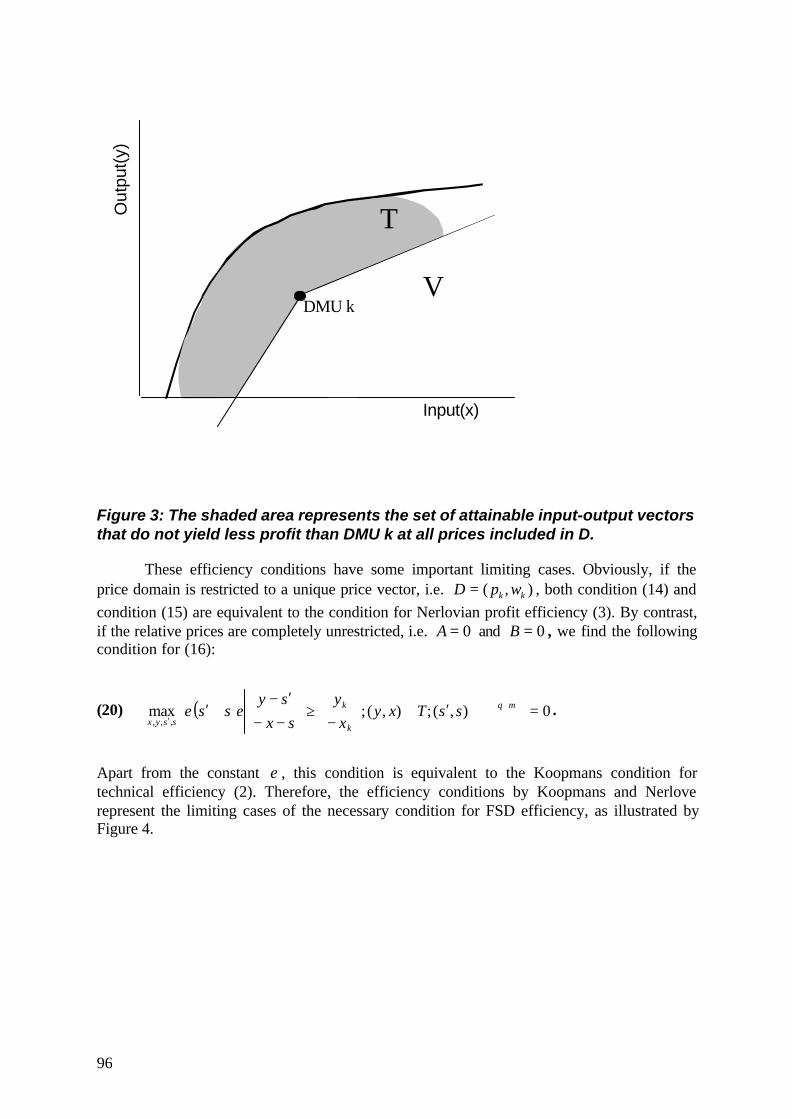
96

Out

put(

y)

Input(x)

T

V DMU k

Figure 3: The shaded area represents the set of attainable input-output vectorsthat do not yield less profit than DMU k at all prices included in D.

These efficiency conditions have some important limiting cases. Obviously, if theprice domain is restricted to a unique price vector, i.e. ),( kk wpD = , both condition (14) andcondition (15) are equivalent to the condition for Nerlovian profit efficiency (3). By contrast,if the relative prices are completely unrestricted, i.e. 0=A and 0=B , we find the followingcondition for (16):

(20) ( ) 0),(;),(;max,,,

=

ℜ∈′∈

−

≥

−−

′−′ +

+′

mq

k

k

ssyxssTxy

xy

sxsy

essε .

Apart from the constant ε , this condition is equivalent to the Koopmans condition fortechnical efficiency (2). Therefore, the efficiency conditions by Koopmans and Nerloverepresent the limiting cases of the necessary condition for FSD efficiency, as illustrated byFigure 4.

97

Out

put (

y)

Input (x)

Koopmans FSD Nerlove

U

DMU k

T

Figure 4: Koopmans technical efficiency and Nerlovian profit efficiency aslimiting cases of the necessary condition for FSD efficiency.

4. Empirical tests

Resorting to the above FSD conditions can reduce the information requirement for thepreference structure and the price distribution. However, information on the production set isstill required. Unfortunately, one typically faces imperfect information on the productionpossibilities in the empirical analysis of production data. However, empirical tests can beobtained approximating the true production set by particular empirical production setconstructed from empirical data.

Various approximations can be employed, depending on the assumptions imposed onthe production set and the data used for approximating it. In Banker, Charnes and Cooper(1984) three key assumptions were imposed. Firstly, the production set was assumed tocontain all observations, i.e.:

(21) .),( TYX ∈

Furthermore, the production set was assumed to satisfy free disposability, i.e.:

(22) 1212222211 ;:),(),(),( xxyyxyTxyTxy ms ≥≤ℜ∈∀∈⇒∈ ++ .

Finally, the production set was assumed convex, i.e.:

98

(23) nTTT eTXYTXY +ℜ∈=∀∈⇒∈ λλλλλ ,1:),(),( .

Banker et al. (1984) used the convex hull of observations as an empirical productionset. The convex hull satisfies the so-called minimum extrapolation principle, being thesmallest set in mq +

+ℜ consistent with the above assumptions. More formally, the followingempirical production set was used to approximate the true production set:

(24) ;1;),(ˆ

ℜ∈=

−≤

−

ℜ∈= ++

+nT

T

Tmq

BCC eX

Yx

yxyT λλ

λλ

.

This empirical production set has become the standard approximation for T in thenonparametric literature. For example, it was used by Banker et al. (1984) and Charnes et al.(1985), among others, for testing and measuring Koopmans' technical efficiency. In addition,Varian (1984), Banker and Maindiratta (1988), and Färe and Grosskopf (1997), amongothers, used it for testing and measuring Nerlovian profit efficiency.

An attractive feature of the convex hull is that it can be used for assessing profitefficiency even if the true production set does not satisfy free disposability and convexity. Ifthe true production set violates free disposability or convexity, the convex hull can containinput-output vectors outside the production set. However, profit is concave and monotonic inoutput and input. Therefore, the data set necessarily contains an observation that produces atleast as much profit as an arbitrary vector from the convex hull, i.e.:

(25) :;),(: mpmqkkkjkj xyxwypwxpySj +

++

+ ℜ∈ℜ∈∀−≥−∈∃ λ

1; =

−≤

−

eX

Yx

y TT

T

λλλ

.

Therefore, the convex hull implicitly represents feasible profit levels. Consequently, theproduction set may harmlessly violate free disposability and convexity, provided allobservations are contained within the same production set (21).

However, under uncertainty, the convex hull can approximate the production set onlyif the latter truly is convex. This is because (25) does not imply that the convex hull containsan observation that produces at least as much profit as an arbitrary vector at all prices fromthe price domain. Therefore, the goodness of the convex hull depends on whether theproduction set truly is convex or not. Convexity requires the production technology to exhibitparticular theoretical characteristics such as non-increasing marginal products and non-increasing marginal rates of substitution and transformation (Madden, 1986). From empiricalpoint of view, little evidence on these theoretical characteristics has been presented (Brue,1993). In case of violations, an alternative empirical production set is required. A number ofalternative sets that do not require convexity have been proposed in the DEA literature,including Deprins, Simar, and Tulkens (1984), Petersen (1990), and Bogetoft (1996).

Figure 5 illustrates this point graphically. The shaded area represents the intersectionof the convex hull of the observations and the polyhedral cone U. This intersection is non-

99

empty, so the necessary condition (16) implies DMU k has to be inefficient. However, theintersection of U and the true, non-convex production set T is empty. Thus, DMU k canactually maximise expected utility. Therefore, if T is non-convex, the convex hullapproximation may lead to erroneous conclusions.

Out

put(

y)

Input(x)

T

U

DMU 1

DMU 2

DMU k TBCC

Figure 5: The shaded area represents the intersection of the convex hull ofobservations and the polyhedral cone U. This intersection is non-empty,falsely implying inefficiency of DMU k.

In contrast to convexity, free disposability can be imposed without harm. This isbecause the data set necessarily contains an observation that yields at least as much profit, atall possible prices, as an arbitrary feasible input-output vector that produces less output anduses more input than the observation, i.e.:

(26) :),(;),(: TxyDwpxwypwxpySj jj ∈∈∀−≥−∈∃ .

−

≤

− j

j

xy

xy

The smallest subset of mq ++ℜ consistent with the assumptions of containment of

observations (21) and free disposability (22) is the so-called Free Disposable Hull (henceforthFDH) set by Deprins et al. (1984) (see also Tulkens, 1993). More formally, the FDH set canbe represented by:

(27) };1,0{;1;),(ˆ

∈∈=

−≤

−

ℜ∈= ++ Sje

XY

xy

xyT jT

T

Tmq

FDH λλλ

λ.

100

Substituting that set for the true production set in the necessary FSD condition (16)gives the following empirical condition:

(28) ( ) ( ){ } ⇔=ℜ∈′∈∈+′−′ ++′

0),(;ˆ),(;,max,,,

mqFDH

ssxyssTxyUsxsyessε

( ) 0;),(;}1,0{;1;max,,,

=

ℜ∈ℜ∈′∈∈=

+−

+≥

−−

′−′ +

++′

lmqj

T

k

kT

T

zsszssSje

zBxzAy

sXsY

ess λλλ

λε

λ

If the observations are contained within the production set, this measure gives a necessarycondition for optimal production under uncertainty.

Similarly, substituting the FDH set for the true production set in the sufficient FSDcondition (15) gives the following empirical condition:

(29) { } ⇔=∈∈−−− 0ˆ),(;),()()(max,,,

FDHkkwpxy

TxyDwpwxpyxwyp

{ } 0}1,0{;1;,;0)()(max,,,

=∈∈=≥≥−−−−′

SjewpBwApwxpyXwYp jT

kkTT

zssλλελλ

λ.

Since the FDH set typically is smaller than the true production set, this condition does notgive a sufficient condition for optimal production. However, it does give a sufficientcondition for dominance over all observations in the sample. Solving a Mixed Integer-LinearProgramming problem for each DMU can check these conditions.

Out

put(

y)

Input(x)

DMU 1

U

DMU 2

DMU 3

DMU k

TFDH

Figure 6: The shaded area represents the intersection of the FDH productionset and the polyhedral cone U. Although DMU k produces on the frontier of thetrue technology, it does not maximize expected utility as there exist observedpoints that yield higher profit at all possible prices.

101

Figure 6 illustrates the application of the FDH set to test the empirical FSD condition(28). The shaded area represents the intersection of the FDH production set and thepolyhedral cone U. Although DMU k produces on the frontier of the true technology, andhence is Koopmans efficient, it does not maximize expected utility as there exist observedpoints that yield higher profit at all possible prices

5. Concluding remarks

We have presented an approach based on first-order stochastic dominance thatextends the nonparametric efficiency analysis to deal with uncertainty related to input-outputprices. We have derived necessary and sufficient first-order stochastic dominance conditionsthat production vectors must satisfy in order to maximise expected utility. Interestingly, thenecessary FSD efficiency condition contains the well-established conditions for Koopmanstechnical efficiency and Nerlovian profit efficiency as its limiting cases.

In addition, we have discussed empirical conditions that can test whether observedbehaviour is consistent with expected utility maximisation. These conditions can be checkedusing standard mathematical programming techniques. A complication for testing FSDempirically is that convexity for the production set cannot be assumed without harm.Therefore, if violations of convexity are anticipated, the FDH set is preferred to the convexhull, which is typically used for testing profit efficiency conditions. From a methodologicalpoint of view, the approach adopted in this paper provides a powerful economic justificationfor the FDH approximation of technology set. We believe a substantial proportion of theappeal related to the convex monotone hull is due to the well-known economicunderpinnings, i.e. the property (25). One important implication of this paper is that theconvenient microeconomic properties of the convex monotone hull can be seriously inflatedin a case of price uncertainty.

Nevertheless, it should be understood that the FSD approach is not limited toparticular empirical production sets. Alternative empirical approximations or estimationscould be used, depending on the purposes of the application and the available information onthe production relationships.

In this paper, we assumed that input-output quantities are controllable, and we onlyconsidered uncertainty related to the input-output prices. However, in some cases, includingBertrand competition, it is necessary to include uncertainty for the quantities as well.Therefore, the inclusion of uncertainty for the input-output variables is an interesting routefor future research. Furthermore, we only discussed testing efficiency of individual DMUs,given a specific theoretical or empirical production set. However, the problem can be easilyturned around to test properties of the production set, given the set of efficient DMUs, as inVarian (1984).

To preserve the applicability related to the established nonparametric tools, wedeliberately avoided imposing assumptions that could be considered restrictive in any sense.Resorting to first order stochastic dominance allowed us to effectively reduce the informationrequirement on the utility function and price distributions. However, in principle nothingprevents one to apply higher-order stochastic dominance rules. Higher order criteria involvemore discriminating power than lower order ones, because they induce a larger reduction of

102

the set of not-dominated choice alternatives. Nevertheless, that power has to be balancedagainst the stringency of the preference imposed assumptions (e.g. risk aversion for second-order stochastic dominance and decreasing absolute risk aversion for third-order stochasticdominance). Still, extending the FSD approach towards higher-order criteria is anotherinteresting challenge for future research.

References

Allen, R., A. D. Athanassopoulos, R.G. Dyson and E. Thanassoulis (1997): WeightRestrictions and Value Judgements in DEA: Evolution, Development and Future Directions.Annals of Operations Research 73, 13-34.

Banker, R.D., Charnes, A., and W. W. Cooper (1984): Some Models for EstimatingTechnical and Scale Inefficiencies in Data Envelopment Analysis, Management Science 30,No. 9, 1078 - 1092

Banker, R.D. and A. Maindiratta (1988): Nonparametric Analysis of Technical andAllocative Efficiencies in Production, Econometrica 56 (6), 1315-1332.

Bertrand, J. (1883): Théorie Mathématique de la Richesse Sociale, Journal des Savants, 499 -508

Bogetoft, P. (1996): DEA on Relaxed Convexity Assumptions, Management Science 42, 457-465.

Brue, S.L. (1993): Retrospectives: The Law of Diminishing Returns, Journal of EconomicPerspectives, 7 (3), 185-192.

Charnes, A., W. Cooper, Z. M. Huang and D. B. Sun (1990): Polyhedral Cone-ratio DEAModels with an Illustrative Application to Large Commercial Banks, Journal ofEconometrics 46, 73-91.

Charnes, A., W. Cooper, and E. Rhodes (1978): Measuring the Efficiency of DecisionMaking Units, European Journal of Operational Research 2, 429 - 444

Charnes, A., W. Cooper, B. Golany, L. Seiford, J. Stutz (1985): Foundations of DataEnvelopment Analysis for Pareto-Koopmans Efficient Empirical Production Functions,Journal of Econometrics, 30, No. 1, 91 – 107

Cournot, A. (1838): Recherches sur les Principes Mathématiques de la Théorie desRichesses. English edition: Researches into the Mathematical Principles of the Theory ofWealth, Edited by N. Bacon, New York, Macmillan

Debreu, G. (1951): The Coefficient of the Resource Utilization, Econometrica 19 (3), 273 -292

Deprins, D., D. Simar, H. Tulkens (1984): Measuring Labor Efficiency in Post Offices, p.243 - 267 in M. Marchand, P. Pestieau and H. Tulkens (Eds.),, The Performance of PublicEnterprises: Concepts and Measurements, North Holland

103

Farrell, M. J. (1957): The Measurement of Productive Efficiency, Journal of the RoyalStatistical Society Series A 120 (3), 253 - 281

Färe, R., and S. Grosskopf (1997): Profit efficiency, Farrell decompositions and the Mahlerinequality, Economics Letters 57, 283-287

Hadar, J. and W. R. Russell (1969): Rules for Ordering Uncertain Prospects, AmericanEconomic Review 59, 25-34.

Levy, H. (1992): Stochastic Dominance and Expected Utility: Survey and Analysis,Management Science 38 (4), 555-593.

Koopmans, T. (1951): Activity Analysis of Production and Allocation, John Wiley & SonsInc., New York

Madden, P. (1986) 'Concavity and Optimisation in Microeconomics', ISBN 0-631-14192-8.

Neumann, J. Von, and O. Morgenstern (1967): Theory of games and economic behaviour,Wiley, New York.

Nerlove, M. (1965): Estimation and Identification of Cobb-Douglas Production Functions,Rand McNally, Chicago, Illinois.

Petersen, N. C. (1990): Data Envelopment Analysis on a Relaxed Set of Assumptions.Management Science, vol. 36 (3), 305-314.

Qin, C.-Z., and Stuart, C. (1997): Bertrand versus Cournot revisited, Economic Theory, vol.10 (3), 497-507

Tulkens, H. (1993): On FDH Efficiency Analysis: Some Methodological Issues andApplication to Retail Banking, Courts, and Urban Transit, The Journal of ProductivityAnalysis, 4, No. 1, 183-210

Varian, H (1984): The Nonparametric Approach to Production Analysis, Econometrica 52(3), 579-597.

104

Appendix 1: Errata

We have identified the following errors in the original articles.

Article II:

Some typing errors are noted:

On p. 53, Section 2, 1st paragraph. "The second difference is that Färe and Svensson phrasedtheir definition in terms of (single- input) production functions…". This should read [(single-output) production functions].

p. 55, Section 4, 3rd paragraph. "It therefore seems more meaningful to compare alternativeDEA models on the level of the assumptions…" [at the level of the assumptions].

Article III:

P. 60, Section 2, 1st paragraph. "Note that this congestion adjustment is harmless as far as theusual (Pareto-Koopmans or Debreu-Farrell) notions of technical efficiency are concerned."This statement is true as for the Pareto-Koopmans notion of technical efficiency, but not so inthe case of Debreu-Farrell notion. See Article II for further details.

P. 63, References: The paper by Diewert was published in 1982 as stated in the text, not in1978 as claimed in the list of references.

Article IV:

Firstly, an annoying technical error. We are grateful to Professor Niels-Christian Petersen forpointing out this technical error in his pre-examination report of this dissertation.

From Article IV (p. 71):

"The price domain cone W involves two sets that are interesting from an economicperspective, and that will prove helpful for approximating economic efficiency. […] Thesecond set contains all input vectors associated with a nonnegative cost at some prices in W:

(3.3) { }: 0 V qW x w W xw= ∈ℜ ∃ ∈ ≥ ."

In Article IV we assumed that this set is equivalent to the following set:

VW% ={ }; ; 0 qix x A i Lα α∈ℜ ≥ ∈ ≥ ,

and proceeded to derive Proof 3.2 and empirical estimator (4.7), formulated in terms of thisset. Unfortunately, the two sets are not equivalent. Example: Consider a case with two inputsand suppose A=0, which implies that VW% 2

+ℜ= . Consider the input vector )11(−=x .Clearly, x does not belong to the set VW% q

+ℜ= . Yet, Vx W∈ since there exist feasible prices

105

at which the cost is positive, e.g. )10(=x . It follows that Proof 3.2 (associated withTheorem 3.2 which still is correct) and the empirical estimator (4.7) are incorrect.

To correct this problem, we can introduce the following alternative set:

{ };V q li i

W x x A i Lα α −= ∈ℜ ≥ ∀ ∈ ℜ ∈ .

In Kuosmanen and Post (2001) we present a revised proof of the Lower Bound Theorem 3.2.,which implies that this set is equivalent to (3.3).

To facilitate empirical application, we proposed an enumerative Linear Programmingprocedure for computing the empirical estimator );,( WyxCE FDHL relative to the Free

Disposable Hull (FDH) input set { }ˆ ( ) ; ;qFDH j jL y x y y x x j S+= ∈ℜ ≤ ≥ ∈ . We next briefly

outline a revised algorithm to correct the error identified above.

To characterize that reference technology, the original article first identified (by enumeration)the subset of observed production plans that yield output vectors greater than or equal to y,i.e. { }( ) j jy x X y yχ = ∈ ≥ . (For notational convenience, in Article IV ( )yχ was used

interchangeably for this discrete set of input vectors, and the matrix consisting of thesevectors.) Since the set ( )yχ necessarily includes all the extreme points of ˆ ( )FDHL y , the lower

bound estimator );,( WyxCE FDHL can equivalently be written in terms of this set as

=);,( WyxCE FDHL { }( )

min min 1j

jw W x yx w xw

χ∈ ∈

=

.

We can next safely reserve the order of the two minimization problems:

=);,( WyxCE FDHL { }( )( )min min 1j

jx y w Wx w xw

χ∈ ∈= .

Thus, the lower bound estimator can be easily computed by the following simple algorithm:1) Identify the input set ( )yχ by enumeration. 2) Solve the embedded LP problems

{ }min 1jw Wx w xw

∈= for each ( )jx yχ∈ . 3) Select the minimum of the optimal solutions to

those problems.

Note: In large-scale applications, the computation burden can be reduced by using additionalinformation (e.g. from technical efficiency classifications, or cost efficiency upper bounds) todecrease the size of ( )yχ by eliminating all 'inefficient' observations that cannot solve thesubsequent minimization problem in Step 3.

To conclude, we happily noticed that actually the correct algorithm outlined above wasoriginally used for computing the lower bound estimates in the empirical applicationpresented in Article IV. The error with the input set was introduced in one of the subsequentrevisions.

106

Finally, there is an error in the references concerning the forthcoming papers Kuosmanen(2000) and Post (2000). Both are scheduled for publication in 2001.

Article V:

p. 101, Section 5, 4th paragraph: "In this paper, we assumed that input-output quantities arecontrollable, and we only considered uncertainty related to the input-output prices. However,in some cases, including Bertrand competition, it is necessary to include uncertainty for thequantities as well." This remark on Bertrand competition takes a shortcut, which may appearconfusing. Actually, the case of Bertrand competition does not directly relate to the quantityuncertainty at all. It merely points to the fact that in some situations it may be moreappropriate to model the prices (rather than quantities) as decision variables, while thedemanded/supplied quantities would be determined by the market forces. In such a setting, itmight be reasonable to associate the uncertainty to the quantities.

References

Kuosmanen, T., and G.T. Post (2001): Notes on: Measuring Economic Efficiency withIncomplete Price Information, an unpublished manuscript

Starmer, C. (2000): Developments in Non-Expected Utility Theory: The Hunt for aDescriptive Theory of Choice under Risk, Journal of Economic Literature 37, 332-382

107

Appendix 2: Examples

Details of the two examples discussed in Article II.

Example 1:

DMU Output y Input x1 Input x2

1 2 1 22 2 2 23 2 2 14 2 1 35 2 1 46 2 3 1.257 2 4 1.25

Source: Färe, R., S. Grosskopf, and C.A.K. Lovell (1985): The Measurement of Efficiency ofProduction, Kluwer Academic Publishers, Boston

73

1

4

5

6

2

0

1

2

3

4

5

0 1 2 3 4 5

x1

x2

108

Example 2:

DMU Output y Input x1 Input x2

A 1 5 1B 1 1 5C 1 5 10D 1 10 5G 1 7.5 7.5R 10 5 5

Source: Brockett, P.L., W.W. Cooper, H.C. Shin, and Y. Wang (1998): Inefficiency andCongestion in Chinese Production Before and After the 1978 Economic Reforms, Socio-Economic Planning Sciences 32, 1-20

C(5,10)

R(5,5)

B(1,5)

A(5,1)

D(10,5)

G(7.5,7.5)

0

2

4

6

8

10

12

0 2 4 6 8 10 12

x1

x2