the role of remote sensing in assessing the...
TRANSCRIPT
UNIVERSIDADE DE LISBOA FACULDADE DE CIÊNCIAS
DEPARTAMENTO DE ENGENHARIA GEOGRÁFICA, GEOFÍSICA E ENERGIA
THE ROLE OF REMOTE SENSING IN ASSESSING THE IMPACT OF CLIMATE VARIABILITY ON VEGETATION
DYNAMICS IN EUROPE
Célia Marina Pedroso Gouveia
Doutoramento em Ciências Geofísicas e da GeoInformação
(Detecção Remota)
2008


UNIVERSIDADE DE LISBOA FACULDADE DE CIÊNCIAS
DEPARTAMENTO DE ENGENHARIA GEOGRÁFICA, GEOFÍSICA E ENERGIA
THE ROLE OF REMOTE SENSING IN ASSESSING THE IMPACT OF CLIMATE VARIABILITY ON VEGETATION
DYNAMICS IN EUROPE
Célia Marina Pedroso Gouveia
Doutoramento em Ciências Geofísicas e da GeoInformação
(Detecção Remota)
Tese orientada pelo Professor Doutor Carlos da Camara, Professor Associado do Departamento de Física da Faculdade de Ciências da Universidade de Lisboa e pelo Professor Doutor Ricardo Machado Trigo,
Investigador Auxiliar do Instituto D. Luiz
2008


ACKNOWLEDGEMENTS
to my father


- i -
ACKNOWLEDGEMENTS My first words of acknowledgment are for my supervisors. To Prof. Carlos da Camara I
am grateful for accepting being my supervisor and for introducing me into Remote
sensing; indeed, I have learned more than advanced techniques of colouring! His words
of friendship, never-ending optimism and senses of humour made this work much more
interesting. Our science-related discussions, his advices and suggestions, made me
‘grow up’.
I am especially indebted to Prof. Ricardo Trigo to whom I thank the support, dedication,
involvement and suggestions; that without them this work would not have ever arrived
to a safe harbour. His words and friendship in crucial moments of this long way showed
me the light at the end of the tunnel.
To my PhD colleague and friend, Margarida L. R. Liberato, I thank her unconditional
friendship, patience and support, our long and fruitful scientific discussions, which
helped overcoming difficulties.
I may not forget Teresa Calado, to whom I thank her suggestions, friendship and
support, which eased this work. To Dulce Lajas I thank for her friendship and support,
so important at the initial stage of this research. To Renata Libonati and Leonardo Peres
I thank our scientific discussions so important that proved that friendship is at the
distance of a click. I also would like to thank Alexandre Ramos, Joana Freire, Telmo
Frias and David Barriopedro for their friendship.
I am grateful to Escola Superior de Tecnologia and Instituto Politécnico de Setúbal,
where I have been teaching since 1999, for granting a six-month leave for full time
scientific research, so important at the final stage of this work, as well as for supporting
my participation at International Scientific Conferences and Workshops where I have
presented scientific results from this research. A word of acknowledgment is also due to
my colleagues at the Departamento de Energia Mecânica who have always motivated

- ii -
me to pursue these studies, in particular Fernando Cunha, Luis Ferro, Luis Coelho and
Miguel Cavique. To Margarida Lopes I thank for her precious teaching collaboration.
Last, but not the least, a very special word of acknowledgement to my family and close
friends for their understanding and help provided during this long path. To Débora and
Miguel for the time we did not spend together, during which they grow and became
adults. To my sister and my parents, for all the motivation incentive encouragement,
help and support they have always provided; without it this work would have been
impossible. A very special thought towards my mother who taught me to dream and
also showed me that depending on our will dreams may become true.
To my husband, Rogério, who has always accompanied me along this course, as along
the other paths, and with whom I have been sharing good and bad moments of all these
years, I wish to thank for all his support, help and love without which all this effort
would not make sense. This work is also a bit of him! To Duarte, who cannot
understand yet why mummy likes doing “such things” so much, I want to thank his
patience, understanding and care for what we could not do together, but mainly for what
we managed to do. These prove that, after all, he has been my master piece (once again
shared with my husband).
Finally, to my Father, who has always believed that I would accomplish this goal and
would certainly have a smile of proud on his lips. Unfortunately he did not live to see
this day. To him, that I miss so much, I dedicate this work.
The Portuguese Foundation of Science and Technology (FCT) partially supported this
research (Grant SFRH / BD / 32829 / 2006).

- iii -
ABSTRACT
The study aims at investigating the relationship between climate variability and
vegetation dynamics by combining meteorological and remote-sensed information. The
vegetation response to both precipitation and temperature in two contrasting areas
(Northeastern Europe and the Iberian Peninsula) of the European continent is analysed
and special attention is devoted to the impact of the North Atlantic Oscillation (NAO)
on the vegetative cycle in the two regions which is assessed taking into account the
different land cover types and the respective responses to climate variability.
An analysis is performed of the impact of climate variability on wheat yield in Portugal
and. the role of NAO and of relevant meteorological variables (net solar radiation,
temperature and precipitation) is investigated. Using spring NDVI and NAO in June as
predictors, a simple regression model of wheat yield is built up that shows a general
good agreement between observed and modelled wheat yield values.
The severity of a given drought episode in Portugal is assessed by evaluating the
cumulative impact over time of negative anomalies of NDVI. Special attention is
devoted to the drought episodes of 1999, 2002 and 2005. While in the case of the
drought episode of 1999 the scarcity of water in the soil persisted until spring, the
deficit in greenness in 2005 was already apparent at the end of summer. Although the
impact of dry periods on vegetation is clearly noticeable in both arable land and forest,
the latter vegetation type shows a higher sensitivity to drought conditions.
Persistence of negative anomalies of NDVI was also used to develop a procedure
aiming to identify burned scars in Portugal and then assess vegetation recovery over
areas stricken by large wildfires. The vulnerability of land cover to wildfire is assessed
and a marked contrast is found between forest and shrubland vs. arable land and crops.
Vegetation recovery reveals to strongly depend on meteorological conditions of the year
following the fire event, being especially affected in case of a drought event.
Keywords: Remote sensing, Vegetation dynamics, Wheat yield, Vegetation recovery,
Burned areas, Climate Variability, North Atlantic Oscillation, Drought persistence.


- v -
RESUMO
Os ecossistemas terrestres têm vindo a ser objecto de interesse crescente devido
ao papel que desempenham no controlo e forçamento do sistema climático à escala
global. Responsáveis pelo armazenamento e libertação de diversos gases com efeito de
estufa, tais como o dióxido de carbono (CO2), o metano e o óxido nitroso, os
ecossistemas terrestres encontram-se, por sua vez, sujeitos localmente à influência do
clima. Tais interacções traduzem-se numa multiplicidade de mecanismos de feedback
entre o ciclo do carbono e o clima, os quais podem ser atenuados ou amplificados pela
variabilidade climática às escalas regional e global. Neste contexto, destaca-se o papel
da vegetação, dada a quantidade elevadíssima de carbono que é armazenada na própria
vegetação e na matéria orgânica.
Recentemente, um número crescente de trabalhos tem vindo a pôr em evidência
a resposta das componentes terrestres do ciclo do carbono às variações e tendências do
sistema climático à escala global. Heimann e Reichstein (2008) mostraram que a forte
variabilidade interanual da taxa global de crescimento médio de CO2 atmosférico está
correlacionada fortemente com o índice El-Niño-Oscilação do Sul. Este controlo parece
estar relacionado com o impacto de eventos extremos na vegetação da Amazónia
ocidental e do sudeste da Ásia, conduzindo a uma perda do carbono pela floresta devido
à diminuição da produtividade fotossintética e/ou ao aumento da respiração.
Ao estudar o impacto do clima no balanço do carbono assume-se que a
sequestração de CO2, pela fotossíntese, é estimulada pelo aumento de temperatura e
pelo próprio aumento de CO2 (Davidson e Janssens, 2006), tendo-se que estes processos
– que ocorrem essencialmente nas florestas da região boreal e das regiões temperadas –
devem atingir a saturação para valores elevados da temperatura e da concentração de
CO2. Acontece, porém, que a respiração responde de forma exponencial às variações da
temperatura, mas não é sensível aos níveis do CO2. Assim, parece ser a própria biosfera
que fornece um mecanismo de feedback negativo para o aumento da temperatura e do
CO2, o qual permanecerá activo enquanto o efeito de estimulação da temperatura
exceder o efeito de fertilização do CO2 (Denman et al., 2007). Por outro lado, numa
terra aquecida, será de esperar um aumento da evaporação, conducente a um balanço

- vi -
negativo da água, o qual será mitigado pela diminuição da perda da água nos estomas
das plantas, característica de um mundo com excesso de CO2. Desta forma, o resultado
líquido dependerá essencialmente da capacidade de armazenamento de água pelo solo,
da distribuição vertical do carbono e das raízes no solo e da sensibilidade geral da
vegetação às condições de stress hídrico (Heimann e Reichstein, 2008), tendo-se que as
limitações em água podem até suprimir a resposta da respiração à temperatura.
(Reichstein et al., 2007). Sob condições de seca severa, alguns cenários climáticos
apontam para um aumento do sequestro do carbono através da supressão da respiração,
bem como da redução da perda de carbono devido à diminuição da actividade
fotossintética (Ciais et al., 2005; Saleska et al., 2003).
Acontece que a biosfera não responde unicamente às variações das variáveis
climáticas médias, mas também – e sobretudo – às flutuações e à variabilidade dessas
variáveis, as quais, por sua vez, se encontram relacionadas com a ocorrência de eventos
extremos. Um bom exemplo desta dependência foi a recente onda de calor que assolou a
Europa durante o Verão de 2003; tendo-se que a acumulação de carbono durante os
cinco anos precedentes, foi anulada em apenas alguns dias de condições atmosféricas
extremas. Ciais et al. (2005) mostraram que a respiração, em vez de aumentar com a
temperatura, diminuiu juntamente com a produtividade, tendo aqueles autores destacado
ainda que as secas e as ondas de calor podem modificar a produtividade da vegetação e
transformar, por curtos períodos, sumidouros em fontes, conduzindo, desta forma, a um
mecanismo de feedback positivo do sistema climático. Os efeitos prejudiciais de tais
eventos extremos podem mesmo ser amplificados por meio de impactos retardados, tais
como aqueles associados à morte das árvores e à recuperação lenta da vegetação em
caso de incêndios florestais (Heimann e Reichstein, 2008; Le Page et al., 2008).
Nas latitudes elevadas, as variações na sazonalidade da temperatura têm vindo a
induzir Invernos amenos e Primaveras antecipadas, conduzindo a um derretimento dos
gelos e a um florescimento da vegetação prematuros e, portanto, a uma maior
vulnerabilidade às geadas (Myneni et al., 1997; Zhou et al., 2001). Por outro lado, os
aumentos de temperatura observados, na Primavera e no Outono das latitudes elevadas
do Hemisfério Norte, conduzem a um aumento da extensão da estação de crescimento e
a uma maior actividade fotossintética, a qual poderá afectar o ciclo sazonal do carbono.
Enquanto que na Primavera a fotossíntese prevalece sobre a respiração, já no Outono
acontece o oposto e, por conseguinte, será na Primavera que se espera a ocorrência do
sequestro de CO2 (Piao et al., 2008). No futuro – e caso se verifique um aquecimento

- vii -
mais acelerado no Outono – a capacidade de sequestro do carbono pelos ecossistemas
do Norte poderá diminuir mais rapidamente do que se previa (Sitch et al., 2008).
Por sua vez, as variações temporais na velocidade de vento, na temperatura do
ar, no stress hídrico e na humidade podem induzir variações na frequência e na
severidade dos fogos florestais e, consequentemente, originar a libertação para a
atmosfera, em apenas alguns minutos, de enormes quantidades do carbono, que foram
acumuladas no solo e na vegetação durante séculos (Shakesby et al., 2007; Michelsen et
al., 2004). Acresce que fogos florestais mais frequentes e mais intensos reduzem a
biomassa e a produtividade da camada superficial do solo, o que leva à erosão e à
diminuição do biodiversidade e, em última análise, conduzirá à degradação dos solos.
Por outro lado, em regiões áridas e semi-áridas, e durante períodos secos, as espécies
herbáceas altamente combustíveis tendem a competir com a vegetação nativa, tornando
estas áreas mais vulneráveis ao fogo, devido à acumulação de biomassa seca altamente
inflamável. Por sua vez, a reincidência de incêndios pode induzir alterações na estrutura
do coberto vegetal, convertendo a vegetação nativa em espaços florestais degradados.
A detecção remota afigura-se presentemente como uma ferramenta muito útil
para a monitorização, à escala global e a custo relativamente baixo, da dinâmica e do
stress da vegetação, bem como da desflorestação e das alterações na utilização do solo.
O aparecimento de novas plataformas, sensores e satélites tem vindo a suscitar um
esforço notável com vista ao desenvolvimento de métodos mais sofisticados e de
algoritmos mais aperfeiçoados com o objectivo de proceder a uma homogeneização das
séries temporais e de integrar observações da natureza diferente. Um bom exemplo é
dado pelo Global Inventory Monitoring and Modelling System (GIMMS), que
proporciona actualmente à comunidade científica mais de vinte anos de dados com 8 km
de resolução, baseados na informação proveniente dos satélites da série
AVHRR/NOAA. A Europa, por sua vez, encetou uma iniciativa complementar, através
do sistema VEGETATION que, desde o final de 1998, tem vindo a fornecer dados
acerca das características da superfície do solo, com 1 km de resolução, baseada na
informação proveniente do sensor VEGETATION a bordo dos satélites SPOT. De
referir, ainda, o esforço adicional que tem vindo a ser efectuado no sentido de se
proceder ao desenvolvimento de diversos índices da vegetação – de que merece
destacar-se o NDVI – elaborados especificamente para quantificar diversos aspectos
relacionados com as concentrações da vegetação verde e a identificação de locais onde a
vegetação é saudável ou se encontra sujeita a stress térmico ou hídrico.

- viii -
A presente tese tem por objectivo contribuir para uma melhor compreensão do
impacto da variabilidade climática na dinâmica da vegetação à escala europeia, com
especial ênfase nos aspectos particulares que ocorrem em Portugal continental e dando-
se especial atenção à análise da relação entre a actividade fotossintética e a Oscilação do
Atlântico Norte (NAO) já que esta constitui o modo principal de variabilidade climática
do Hemisfério Norte. Assim – e no seguimento de diversos estudos que abordaram
alguns aspectos da relação da NAO com a dinâmica da vegetação à escala europeia
(D’Odorico et al., 2002; Cook et al., 2004; Stöckli and Vidale, 2004; Vicente Serrano
and Heredia Laclaustra, 2004) – procedeu-se a uma análise sistemática de duas regiões
com comportamentos contrastantes, a saber a Península Ibérica e o Nordeste da Europa.
A análise, que abarcou um período de 21 anos (1982-2002), foi efectuada a partir de
compósitos mensais de NDVI e da temperatura do brilho da série de dados GIMMS,
bem como da precipitação mensal disponibilizada pelo Global Precipitation
Climatology Centre (GPCC). Para o referido período de 21 anos, procedeu-se a um
estudo sistemático dos campos de correlação pontual entre os valores de Inverno da
NAO e os correspondentes valores da Primavera e do Verão do NDVI, tendo-se ainda
analisado, nas duas regiões referidas, a resposta da vegetação às condições de
precipitação e de temperatura de Inverno. No caso da Península Ibérica, os resultados do
estudo efectuado evidenciaram que valores (negativos) positivos da NAO de Inverno
induzem (elevada) baixa actividade da vegetação na Primavera e no Verão seguintes,
estando este comportamento associado ao impacto da NAO na precipitação do Inverno,
conjuntamente com a forte dependência da vegetação da Primavera e do Verão da
disponibilidade de água durante o Inverno precedente. Já no Nordeste da Europa se
observou um comportamento diferente, com valores (negativos) positivos da NAO de
Inverno a induzirem valores (baixos) elevados de NDVI na Primavera e valores
(elevados) baixos de NDVI no Verão, comportamento este resultante principalmente do
forte impacto da NAO na temperatura do Inverno, associado com a dependência do
crescimento da vegetação do efeito combinado de condições amenas e da
disponibilidade de água ocorridas no Inverno. Na Península Ibérica, observou-se ainda
que o impacto da NAO é maior nas zonas não florestadas, já que estas respondem mais
rapidamente às variações espaço-temporais da humidade do solo e da precipitação. No
Nordeste da Europa, o impacto da NAO é especialmente notório durante os primeiros
meses do ano, sugerindo que o crescimento da vegetação verde tende a ocorrer mais

- ix -
cedo e intensamente nos anos de fase positiva da NAO, devido às condições
relativamente mais amenas associadas a um derretimento prematuro do coberto de gelo.
Os resultados obtidos – em particular aqueles que respeitam à relação entre a
NAO de Inverno e o NDVI da Primavera e do Verão – representam um importante valor
acrescentado, na medida em que proporcionam uma antevisão global do estado da
vegetação, passível de diversas aplicações que incluem a formulação de previsões a
curto prazo da produtividade de culturas e a previsão a longo prazo de risco de
incêndios florestais. Neste contexto – e no seguimento de diversos estudos em que se
procede ao estudo de relações entre o rendimento de culturas e a distribuição espaço-
temporal de variáveis meteorológicas relevantes (Maytelaube et al. 2004; Atkinson et
al., 2005; Iglesias and Quiroga, 2007, Rodríguez-Puebla et al., 2007) – analisou-se a
produtividade de trigo no Alentejo e suas relações com o regime meteorológico do ano
agrícola. O estudo foi suscitado pelo facto de se terem encontrado no Alentejo, para o
período 1982-1999, correlações fortemente negativas entre a produtividade do trigo e o
NDVI da Primavera obtido a partir da base de dados GIMMS. O impacto dos factores
meteorológicos na produtividade do trigo naquela região foi, por sua vez, avaliado
através do cálculo de correlações mensais das anomalias da produtividade do trigo com
a radiação solar, a temperatura e a precipitação, bem como com a NAO. Os resultados
obtidos indicam que temperaturas frias durante o Inverno e uma Primavera antecipada,
juntamente com a ocorrência de precipitação em Fevereiro e Março e a disponibilidade
de radiação solar em Março, têm um impacto positivo durante a fase de crescimento,
tendo-se ainda que um valor elevado do índice NAO em Junho é benéfico para o estádio
de maturação do grão. Com base nas relações obtidas, procedeu-se à elaboração de um
modelo simples (de regressão linear multivariada) da produção de trigo, utilizando
como predictores os valores de NDVI da Primavera e da NAO de Junho. Os resultados
da validação cruzada confirmaram o bom desempenho do modelo, que se antevê possa
vir a ser melhorado quando estendido a um período mais alargado.
Os campos de NDVI derivados do sensor VEGETATION foram, por sua vez,
utilizados para monitorizar episódios de seca em Portugal continental, estudo este
motivado pelo recente reconhecimento da existência de uma forte dependência da
dinâmica da vegetação, na região do Mediterrâneo, da disponibilidade em água
(Eagleson, 2002, Rodríguez-Iturbe and Porporato, 2004, Vicente-Serrano and Heredia-
Laclaustra, 2004, Vicente-Serrano, 2007). Nesta conformidade, a severidade de um
dado episódio de seca foi avaliada através da persistência temporal das condições de

- x -
stress hídrico da vegetação – traduzida pelo número de meses em que se observa uma
anomalia negativa do NDVI num determinado período de tempo – tendo-se dado
atenção especial ao episódio de seca de 2005, bem como aos episódios ocorridos em
1999 e em 2002. O impacto da humidade do solo na dinâmica da vegetação foi ainda
avaliado através do estudo do ciclo anual do Soil Water Index (SWI) em função do
NDVI, tendo-se observado que, no caso do ano de 1999, a escassez de água no solo
persistiu até à Primavera, enquanto que, no episódio de 2005, o stress da vegetação já
era visível no final do Verão. Igualmente se avaliou o impacto dos períodos secos nos
diferentes tipos de coberto vegetal, tendo-se observado, em particular, que a terra arável
apresenta maior sensibilidade do que a floresta.
O problema da recuperação da vegetação após um episódio de fogo florestal tem
vindo a ser objecto de um considerável número de estudos realizados para as regiões do
Mediterrâneo e baseados em informação proveniente de detecção remota (Jakubauskas
et al., 1990; Viedma et al., 1997; Díaz-Delgado et al., 1998; Henry and Hope, 1998;
Ricotta et al., 1998). Seguindo o exemplo de alguns autores que têm utilizado o NDVI
para proceder à monitorização da recuperação do coberto vegetal (Paltridge and Barber,
1988; Viedma et al., 1997; Illera et al., 1996), novamente se recorreu à persistência das
anomalias negativas de NDVI para simultaneamente desenvolver uma metodologia que
permitisse a identificação de áreas queimadas e avaliasse a capacidade de recuperação
da vegetação nas áreas ardidas. A metodologia desenvolvida revelou-se adequada para
ambos os propósitos no caso de áreas afectadas por incêndios florestais de grandes
dimensões, tendo os resultados obtidos apontado para uma muito maior vulnerabilidade
ao fogo das zonas de floresta e de mato, em contraste com o observado nas zonas de
terra arável e culturas. No que respeita à recuperação da vegetação nas áreas afectadas
por fogos florestais, observou-se que a recuperação depende em larga medida das
condições meteorológicas durante o ano que se segue ao fogo, em particular das
condições de aridez. De facto, verificou-se que a recuperação da vegetação foi
especialmente lenta em 2003, por causa da seca que se seguiu em 2004/2005, sobretudo
nas áreas ardidas na região do Algarve onde os efeitos da seca foram mais severos.
Palavras chave: Detecção Remota, Dinâmica da Vegetação, Produtividade do Trigo em
Portugal, Recuperação da Vegetação, Áreas Ardidas, Variabilidade Climática,
Oscilação do Atlântico Norte, Secas, Severidade, Persistência de Secas

- xi -
TABLE OF CONTENTS
Acknowledgements...........................................................................................................i
Abstract...........................................................................................................................iii
Resumo.............................................................................................................................v
Table of Contents............................................................................................................xi
List of Figures................................................................................................................xv
List of Tables...............................................................................................................xxiii
List of Acronyms..........................................................................................................xxv
1. Introduction ........................................................................................................ xxv
2. Fundamentals.......................................................................................................... 7
2.1 Remote sensing................................................................................................. 7
2.2 Radiometric concepts ....................................................................................... 8
2.3 Image correction............................................................................................. 12
2.3.1 Atmospheric correction .......................................................................... 12
2.3.2 Radiometric correction ........................................................................... 14
2.3.3 Geometric correction .............................................................................. 14
2.3.3.1 Distortion models ............................................................................... 16
2.3.3.2 Coordinate transformations ................................................................ 17
2.4 Resampling ..................................................................................................... 22
2.5 The SPOT and the NOAA systems ................................................................ 24
2.5.1 The SPOT Program ................................................................................ 24
2.5.2 The NOAA series ................................................................................... 31
3. Basic Data and Pre-Processing............................................................................ 35
3.1 Vegetation Indices .......................................................................................... 35
3.1.1 Introduction ............................................................................................ 35

- xii -
3.1.2 Performance and limitations of empirical vegetation indices ................ 37
3.1.3 NDVI from AVHRR/NOAA.................................................................. 40
3.1.4 NDVI data fromVEGETATION/SPOT ................................................. 42
3.2 Land Cover Maps ........................................................................................... 45
3.2.1 Introduction ............................................................................................ 45
3.2.2 The Global Land Cover 2000 Project..................................................... 45
3.2.3 The Corine Land Cover 2000 project ..................................................... 47
3.3 Climate data.................................................................................................... 53
3.3.1 Meteorological Data ............................................................................... 53
3.3.2 North Atlantic Oscillation ...................................................................... 54
4. Climate Impact on Vegetation Dynamics........................................................... 57
4.1 Introduction .................................................................................................... 57
4.2 Methodology................................................................................................... 60
4.3 NAO and Vegetation Greenness..................................................................... 62
4.4 NAO and Climatic Activity............................................................................ 65
4.5 The role NAO on the vegetative cycle ........................................................... 73
4.6 Conclusions .................................................................................................... 75
5. Interannual Variability of Wheat Yield in Portugal ......................................... 79
5.1 Introduction .................................................................................................... 79
5.2 Wheat and Climate ......................................................................................... 81
5.3 Wheat in Portugal ........................................................................................... 82
5.3.1 Production and Yield .............................................................................. 83
5.3.2 Vegetative cycle ..................................................................................... 85
5.3.3 Spatial distribution.................................................................................. 86
5.3.4 Meteorological variables ........................................................................ 88
5.4 A simple regression model for wheat yield .................................................... 93
5.5 Final Remarks................................................................................................. 95
6. Drought and Vegetation Stress Monitoring ....................................................... 97
6.1 Introduction .................................................................................................... 97
6.2 Vegetation stress............................................................................................. 99
6.3 Drought assessment ...................................................................................... 101
6.3.1 Annual cycle of NDVI.......................................................................... 101
6.3.2 Annual cycle of soil moisture............................................................... 105
6.4 Drought persistence ...................................................................................... 112

- xiii -
6.5 Final remarks ................................................................................................ 118
7. Monitoring Burned Areas and Vegetation Recovery...................................... 123
7.1 Introduction .................................................................................................. 123
7.2 Rationale....................................................................................................... 124
7.3 Vegetation recovery in burned areas ............................................................ 128
Final remarks ............................................................................................................ 131
8 Conclusions ......................................................................................................... 135
REFERENCES ........................................................................................................... 139

- xv -
LIST OF FIGURES Figure 2.1 Data collection by remote sensing (from http://www.cla.sc.edu/geog/cgisrs/).
.................................................................................................................................. 8
Figure 2.2 Spatial and temporal resolution for selected remote sensing applications
(from Jensen, 2007). ............................................................................................... 10
Figure 2.3 Spectral reflectance of vegetation (from
http://www.csc.noaa.gov/products/sccoasts/html/images/reflect2.gif ). ................ 11
Figure 2.4 Spectral reflectance of vegetation, soil and water (from
http://landsat.usgs.gov/resources/remote_sensing/remote_sensing_applications.php
)............................................................................................................................... 12
Figure 2.5 Conventional definitions for the three attitude axes of a sensor platform
(source: Schowengerdt, 1997) ................................................................................ 16
Figure 2.6 Ellipsoid, geoid and topographic surfaces (source:
http://www2.uefs.br/geotec/topografia/apostilas/topografia(1).htm ) .................... 19
Figure 2.7 The UTM Zone 29 (source: www.isa.utl.pt/der/Topografia/cartografia2.ppt)
................................................................................................................................ 20
Figure 2.8 Picture of the satellite SPOT 4. (from http://medias.obs-
mip.fr/www/Reseau/Lettre/11/en/systemes/vegetation.html). ............................... 25
Figure 2.9 The cross-track direction operating mode of the two HRV sensors. (from
http://www.spotimage.fr/html/_167_224_230_.php). ............................................ 27
Figure 2.10 Repeated observation by SPOT. (from
http://www.spotimage.fr/html/_167_224_230_.php). ............................................ 27
Figure 2.11 The push broom principle (http://spot4.cnes.fr/spot4_gb/index.htm )........ 28
Figure 2.12 SPOT’s Field of view. (from http://spot5.cnes.fr/gb/satellite/42.htm ) ...... 28
Figure 2.13 The VEGETATION field of view. (from http://spot5.cnes.fr/gb/ .............. 29
Figure 3.1 Reflectance from different wavelengths and different surfaces.................... 35
Figure 3.2 Monthly anomalies of NDVI over Europe for August 2003. Anomalies were
computed with respect to the base period 1999-2004 (excluding 2003)................ 39
Figure 3.3 As in Figure 3.2 but respecting to FAPAR anomalies. Anomalies were
computed with respect to the base period 1998-2002. (from Gobron et al, 2005). 39

- xvi -
Figure 3.4 Monthly time-series of NDVI for the period 1999–2006 and respecting to
four different land cover types; an arable land pixel located in South Alentejo (left
top panel), an arable land pixel located in North Alentejo (right top panel), a
coniferous forest pixel (left bottom panel) and a broad-leaved forest pixel (right
bottom panel). Green dots and the solid curve respectively represent the time series
of corrected and non-corrected NDVI monthly values. ......................................... 43
Figure 3.5 Number of months between September 2001 and August 2002 that are
characterised by NDVI anomaly values below -0.025, using non-corrected (left
panel) and corrected (right panel) NDVI data. ....................................................... 44
Figure 3.6 The Global Land Cover 2000 Project. .......................................................... 46
Figure 3.7 The updated version of the GLC2000 map for the European Window.
(http://www-gvm.jrc.it/glc200 ). ............................................................................ 47
Figure 3.8 Landsat 7 imagery for the updating CLC, using the IMAGINE2000 software.
(http://image2000.jrc.it/ )........................................................................................ 48
Figure 3.9 Corine Land Cover 2000 map for Portugal, as developed by ISEGI and the
adopted 44 class-nomenclature (http://terrestrial.eionet.europa.eu/CLC2000)...... 49
Figure 3.10 Corine Land Cover 2000 map for Portugal; the original map at 250m
resolution (left panel), the degraded map at 1000m resolution using the nearest
neighbour technique (central panel), the degraded map at 1000m resolution using
the majority rule (right panel)................................................................................. 50
Figure 3.11 As in Figure 3.10 but respecting to a box centred in the Tagus estuary. .... 51
Figure 3.12 Histogram of relative frequencies of pixels in the 250m original map (blue),
and in the 1000m degraded maps as obtained using the nearest neighbour
technique (green) and the majority rule (red). Labels in bars identify classes
referred to in the text. ............................................................................................. 51
Figure 3.13 Spatial distribution of relative presence for a set of five GLC2000 classes
for the 1000m degraded maps using the majority rule, respectively urban areas
(code 1.1.2), non irrigated arable land (code 2.1.1), broad-leaved forest (code
3.1.1), water courses (code 5.1.1) and estuaries (code 5.2.2)................................. 52
Figure 3.14 Patterns of simple correlation computed over the period 1982-2002 of three-
monthly averages of winter NAO (JFM) vs. winter precipitation (top panel) and
surface air temperature (bottom panel)................................................................... 56
- xvii -
Figure 4.1 Interannual variability of late winter NAO index over the 21-year long
period, from 1982 to 2002. Open (black) circles indicate years characterised by
NAO indices above (below) the 3rd (1st) quartile. .................................................. 60
Figure 4.2 Temporal averages of NDVISPR (left panel) and NDVISUM (right panel) over
the period from 1982 to 2002. Gray pixels over land correspond to areas covered
by snow and ice. ..................................................................................................... 61
Figure 4.3 As in Figure 4.2 but for PNAO (left panel) and TNAO (right panel). ............... 62
Figure 4.4 Point correlation fields of NAO vs. NDVISPR (left panel) and NAO vs.
NDVISUM (right panel) over the period from 1982 to 2002. Black frames identify
the Baltic region and the Iberian Peninsula. The colorbar identifies values of
correlation and the two arrows indicate the ranges that are significant at 5% level.
................................................................................................................................ 63
Figure 4.5 Boxplots of simple correlation between three months composite of North
Atlantic Oscillation (NAO) and NDVI for the 2 selected areas (NE and IB). ....... 64
Figure 4.6 Seasonal anomalies of NDVISPR for 1986 (NAO+), 1995 (NAO-) and for
differences between 1995 and 1986 (upper, middle and lower panels, respectively)
over IB and NE (left and right panels respectively). .............................................. 65
Figure 4.7 Point correlation fields of NAO vs. TNAO (left panel) and NAO vs. PNAO
(right panel) over the period from 1982 to 2002. The colorbar shows values of
correlation and the two arrows indicate the ranges that are significant at 5% level.
................................................................................................................................ 66
Figure 4.8 Geographical distribution of sets of selected pixels over the IB (upper
panels), based on the strong values of correlation of NDVISPR (upper left panel)
and NDVISUM (upper right panel) with NAO. Red, green and blue pixels are
respectively associated to forest and shrub, cultivated areas and other types of
vegetation cover. Land cover type (low panel) as obtained from GLC2000) ........ 68
Figure 4.9 As in Figure 4.8 but respecting to NHCP over NE. Red, green and blue
pixels are respectively associated to needle-leaved, evergreen, cultivated and other
types of vegetation cover........................................................................................ 69
Figure 4.10 Dispersion diagrams of NDVISPR (upper panels) and NDVISUM (lower
panels) vs. PNAO (left panels) and TNAO (right panels) for selected pixels over the
IB. Each dot represents a pair of median values of a given set of selected 500
pixels, for a given year of the considered period (1982-2002). Years that belong to
the subset of NAO+ (NAO-) are marked in red (green) and the respective variability
- xviii -
is characterised by means of horizontal and vertical bars indicating the interquartile
ranges...................................................................................................................... 71
Figure 4.11 As in Figure 4.10, but respecting to NE...................................................... 72
Figure 4.12 Annual cycles of monthly values of NDVI for NAO High Correlation
Pixels (NHCP), for spring (upper panel) and summer (lower panel), over IB (left
panel) and NE (right panel). The annual cycles of average NDVI values for the
entire period (1982-2002) are represented by thick solid lines, whereas the annual
cycles of averages for the NAO- (NAO+) subsets are identified by the thin solid
(dashed) curves. Vertical dashed curves delimit the season of the year................. 74
Figure 4.13 As in Figure 4.12, but restricting to the annual cycles of NDVI for the
individual years of 1986 (NAO−) and 1995 (NAO+), respectively represented by
the dashed and the solid lines. ................................................................................ 74
Figure 5.1 Comparison of AVHRR, SPOT and MODIS VIs over Southeastern,
Australia, for February 2003 (Justice, 2005).......................................................... 80
Figure 5.2 Time series of annual wheat yield in Portugal for the period from 1961 to
2005: yield (solid line), general trend (dashed line) and anomalies for detrended
time series (line with asterisks). ............................................................................. 84
Figure 5.3 Contribution of different growing regions of Portugal to total wheat yield for
the period from 1996 to 2003. ................................................................................ 84
Figure 5.4 Percentage of Alentejo’s wheat yield for hard and soft wheat for the period
from 1996 to 2003 .................................................................................................. 85
Figure 5.5 Patterns of simple correlation between spring NDVI composites and wheat
yield in Portugal, for the period of 1982-1999 (left panel); patterns of simple
correlation that are significant at the 99% level (right panel). ............................... 86
Figure 5.6 Pixels coded as “arable land not irrigated” according to Corine2000 for
Portugal. (left panel). Relative frequency of correlation coefficient values between
spring composite of NDVI and wheat yield in Portugal, for pixels coded as arable
land (right panel). ................................................................................................... 87
Figure 5.7 As in Figure 5.5 (left panel), but for the pixels with correlations that are
significant at the 99% level. ................................................................................... 87
Figure 5.8 Time series for the period 1982-1999 of detrended anomalies of wheat yield
in Portugal (green curve) and of spring NDVI averaged over the “wheat-like”
pixels (red curve). Values of wheat yield were normalized by subtracting the mean
and dividing by the standard deviation................................................................... 88
- xix -
Figure 5.9 Patterns of simple correlation between wheat yield in Portugal and the three
most relevant meteorological fields for the period of 1982-1999; top panel: net
short wave radiation; middle panel: surface air temperature; bottom panel:
precipitation. Boxes in the Southern sector delimit the area containing “wheat-like”
pixels....................................................................................................................... 90
Figure 5.10 Patterns of simple correlation, over the Iberian Peninsula, between NAO
averaged for April, May and June and contemporaneous fields of radiation (left
panel), temperature (central panel) and precipitation (right panel) for the
considered period 1982-1999. ................................................................................ 91
Figure 5.11Patterns of simple correlation between wheat yield in Portugal and the three
most relevant meteorological fields for the period of 1982-1999; top panel: net
long wave radiation; middle panel: surface air temperature; bottom panel:
precipitation. ........................................................................................................... 92
Figure 5.12 Time series (1982-1999) of observed (green curve) wheat yield in Portugal
and of corresponding modeled values (red curve) when using a linear regression
model based on spring NDVI and NAO in June (upper panel). Time series (1982-
1999) of residuals and respective 95% level confidence intervals (central panel);
the single outlier (in 1998) is highlighted in red. Time series (1982-1999) of
observed (green curve) wheat yield in Portugal and of corresponding modeled
values (red curve) as obtained from the leave-one-out cross-validation procedure.
................................................................................................................................ 94
Figure 6.1 Monthly time-series (1999–2006) of NDVI averaged over Continental
Portugal for all pixels (black line), for pixels of non-irrigated arable land (red line)
and of pixels of broad-leaved forest (green line). Black arrows indicate the drought
episodes of 1999, 2002 and 2005. .......................................................................... 99
Figure 6.2 Monthly means of NDVI (1999-2006) over Continental Portugal, covering
the period from September to August................................................................... 100
Figure 6.3 NDVI anomalies from September to August respecting to the year of
1998/1999. ............................................................................................................ 102
Figure 6.4 As in Figure 6.3 but respecting to the year of 2001/2002........................... 103
Figure 6.5 As in Figure 6.3 but respecting to the year of 2004/2005........................... 104
Figure 6.6 Monthly time-series (1992–2005) of SWI averaged over Continental
Portugal. Values from January 2001 until August 2003 are missing. Black arrows
indicate the drought episodes of 1999 and 2005. ................................................. 106

- xx -
Figure 6.7 Monthly means of SWI (1992-2005) over Continental Portugal, covering the
period from September to August. ....................................................................... 107
Figure 6.8 Climatological cycle of SWI vs. NDVI. Letters indicate months of the year.
.............................................................................................................................. 108
Figure 6.9 SWI anomalies for January to August respecting to the year 1998/1999. .. 109
Figure 6.10 As in Figure 6.9 but respecting to the year 2004/2005. ............................ 110
Figure 6.11 Annual cycles (red curves) of SWI vs. NDVI for the drought episodes of
1999 (left panel) and 2005 (right panel). The climatological cycle (black curves) is
also presented for reference purposes................................................................... 111
Figure 6.12 Annual cycles of spatially averaged NDVI for each year of the considered
period (1999-2006) over non-irrigated arable land (top panel) and coniferous forest
(bottom panel). The drought episodes of 1999 and 2005 are represented,
respectively, by the curves with circles and asterisks. The line in bold refers to
monthly means over the entire period. ................................................................. 112
Figure 6.13 Percentage of continental Portugal with monthly NDVI anomalies lower
than 0 (red bars) and lower than -0.025 (green bars), from September to August of
2005. The black line represents the percentage of mainland affected by extreme
drought, i.e., with PDSI ≈ -4. The 3-month delay of PDSI relatively to NDVI (as
indicated by the two different horizontal time axes) is worth being noted. ......... 114
Figure 6.14 Number of months between September and August that are characterised by
NDVI anomaly values below -0.025, for each year of the considered period (1999-
2006)..................................................................................................................... 116
Figure 6.15 As in Figure 6.14, but all pixels that are identify as burned areas are masked
.............................................................................................................................. 121
Figure 7.1 Annual burned areas in Continental Portugal (right panel) for the fire season
of 2003 (red pixels) using the criterion of at least 5 months of NDVI anomalies
below -0.075 during the period from September to May of 2004; black pixels refer
to burned scars for the previous fire season of 2002. Annual burned areas in
Continental Portugal (central panel) for the period 2000-2004 as identified from
Landsat imagery. The central panel was adapted from Pereira et al. (2006). ...... 125
Figure 7.2 Annual burned areas in Continental Portugal (left panel) for the fire season of
2004 (red pixels) using the criterion of at least 5 months of NDVI anomalies below
-0.075 during the period from September to May of 2005; black pixels refer to
burned scars for the previous fire season of 2003. Annual burned areas in
- xxi -
Continental Portugal (central panel) for the period 2000-2004 as identified from
Landsat imagery. Annual burned areas in Continental Portugal (right panel) for the
fire season of 2004 (red pixels) using the criterion of at least 7 months of NDVI
anomalies below -0.075 during the period from January to August of 2005; black
pixels refer to burned scars for the previous fire season of 2003. The central panel
was adapted from Pereira et al. (2006). ................................................................ 126
Figure 7.3 Annual burned areas in Continental Portugal (left panel) for the fire season of
2005 (red pixels) using the criterion of at least 5 months of NDVI anomalies below
-0.075 during the period from September to May of 2006; black pixels refer to
burned scars for the previous fire season of 2004. Annual burned areas in
Continental Portugal (central panel) for the year of 2005 as identified from Landsat
imagery. Annual burned areas in Continental Portugal (right panel) for the fire
season of 2005 (red pixels) using the criterion of at least 5 months of NDVI
anomalies below -0.075 during the period from January to June of 2006; black
pixels refer to burned scars for the previous fire season of 2004. The central panel
is courtesy from J.M.C. Pereira. ........................................................................... 127
Figure 7.4 Burned scars for each year of the period 1998-2005 as identified based on
NDVI anomalies ................................................................................................... 129
Figure 7.5 Time series of annual burned areas in Continental Portugal for the period
1998-2005 as obtained from the developed methodology (solid line) and based on
DGRF information (dotted curve). ....................................................................... 130
Figure 7.6 Time series of NDVI for selected pixels in a set of eight large fire scars, each
one corresponding to an event that has occurred in a given year of the 1998-2005.
The location of the selected fire scars is given in the upper panel. ...................... 132
Figure 7.7 Time series of averaged NDVI over three large fire scars, one of them
associated to an event in 2001 and the remaining associated to two events in 2003.
The location of the selected fire scars is given in the upper panel. ...................... 133


- xxiii -
LIST OF TABLES Table 2.1 Regions used in remote sensing. (adapted from
http://www.esa.int/esaEO/SEMLFM2VQUD_index_1_m.html). ........................... 9
Table 2.2 Table of Ellipsoids (Adapted from http://ltpwww.gsf.nasa.gov/
IAS/handbook/hamdbook_htmls/chapter1/chapter1.html) .................................... 18
Table 2.3 Projection plane equations for several common map projections (Moik, 1980).
The latitude of a point on the Earth is ϕ and its longitude is λ . The projected map
coordinates, x and y, are called “easting” and “northing”, respectively. R is the
equatorial radius of the Earth and ε is the Earth’s eccentricity. The subscripted
values of latitude and longitude pertain to the definition of a particular projection
(source: Schowengerdt, 1997)................................................................................ 21
Table 2.4 HRV Spectral Bands.(from
http://www.spotimage.fr/html/_167_224_230_.php). ............................................ 25
Table 2.5 HRVIR Spectral Bands
(fromhttp://www.spotimage.fr/html/_167_224_230_.php).................................... 26
Table 2.6 Orbit characteristics for SPOT 5. ................................................................... 30
Table 2.7 SPOT 5 sensor characteristics. ....................................................................... 30
Table 2.8 General time coverage by satellite. (from
http://www.ngdc.noaa.gov/stp/NOAA/noaa_poes.html)........................................ 31
Table 2.9 NOAA Satellites Orbital Characteristics. (Adapted from
http://www.crisp.nus.edu.sg/~research/tutorial/noaa.htm ).................................... 32
Table 2.10 AVHRR Sensor Characteristics. (from
http://www.crisp.nus.edu.sg/~research/tutorial/noaa.htm)..................................... 33
Table 4.1 Descriptive statistics of the distributions of NDVI anomalies for the sets of
selected pixels associated to forest and shrub, and to cultivated areas, in the cases
of spring and summer over the Iberian Peninsula and the Baltic region. P1, Q1, Q2,
Q3 and P99 respectively denote percentile one, the first quartile, the median, the
third quartile and percentile 99. Percent figures in parenthesis below the land cover
types indicate the fraction of pixels of the considered set associated to that type. 70
- xxiv -
Table 5.1 Correlation values between spring NDVI and wheat yield and respective 95%
confidence intervals and level of significance as obtained for 10,000 bootstrap
samples. .................................................................................................................. 88
Table 5.2 Correlation coefficient values between annual wheat yield and monthly net
long wave radiation, air surface temperature and precipitation (from January to
June) for the pixels coded as arable land not irrigated. Bold values are representing
correlations values that are significant at 95% level and red value is presented the
correlation value significant at 99% level. ............................................................. 89
Table 5.3 As in table 5.1, but respecting to net short-wave radiation, temperature,
precipitation in March and to NAO in June. .......................................................... 92
Table 6.1 Percentage of mainland Portugal stricken by serious drought, i.e., with
monthly NDVI anomalies below -0.025 in more than 9 months (out of 11). ...... 115
Table 6.2 Total amounts and relative proportions of pixels affected by drought for
different land cover types during the drought episodes of 1999, 2002 and 2005. 115
Table 6.3 Cumulative effect of drought conditions for specific land cover types during
the drought episodes of 1999, 2002 and 2005. ..................................................... 118
Table 7.1 Percentage of burned pixels for pixels classified as non irrigated Arable Land,
Forest, Transitional woodland-shrub and Shrubland (using Corine Land Cover
Map 2000, CLC2000) for the fire seasons from the years 1998 to 2005. ............ 130

LIST OF ACRONYMS AVHRR Advanced Very High Resolution Radiometer
CLC2000 Corine Land Cover 2000
CNES Centre National d'Etudes Spatiales
CORINE COoRdinate INformation on the Environment
CRU Climate Research Unit
DFRF Direcção Geral dos Recursos Florestais
EEA European Environment Agency
EMD Empirical Mode Decomposition
ERS European Remote Sensing
FAO Food and Agriculture Organization
GAC Global Area Coverage
GEWEX Global Energy and Water Cycle Experiment
GIMMS Global Inventory Monitoring and Modelling System
GIS Geographical Information System
GLAM Global Agriculture Monitoring
GLC2000 Global Land Cover 2000
GPCC Global Precipitation Climatology Centre
HRPT High Resolution Picture Transmission
HRV High Resolution Visible
HRVIR High Resolution Visible and Infrared
IB IBerian peninsula
IFOV Instantaneous Field of View
INE Instituto Nacional de Estatística
ISEGI Instituto Superior de Estatística e Gestão da Informação
JRC Joint Research Center
LAC Local Area Coverage
LST Local Solar Time
MAM March, April and May

- xxvi -
MODIS MODerate Resolution Imaging Spectroradiometer
MS MultiSpectral mode
MSU Microwave Sounding Unit
MVC Maximum Value Composite
NASA National Aeronautics and Space Administration
NDVI Normalised Difference Vegetation Index
NDVISPR SPRing NDVI
NDVISUM SUMmer NDVI
NE Northeastern Europe
NHCP NAO High Correlated Pixels
NAO North Atlantic Oscillation
NIMA United States National Imagery and Mapping Agency
NIR Near InfraRed
NOAA US National Oceanic and Atmospheric Administration
PAN PANchromatic mode
PDSI Palmer Drought Severity Index
PNAO Precipitation corresponding to the winter NAO index
SPOT Satellite Pour l’Observation de la Terre
SWI Soil Water Index
SWIR ShortWave InfraRed
TIR Thermal InfraRed
TNAO Temperature corresponding to the winter NAO index
TOVS TIROS Operational Vertical Sounder
USDA/FAS United States Department of Agriculture/Foreign Agricultural
Service
UTM Universal Transverse Mercator
VGT VEGETATION
VGT-NDVI NDVI using VGT
VGT-P VGT Physical products
VGT-S VGT Synthesis products
VI Vegetation Index
VIS VISible
WCRP World Climate Research Program
WMO World Meteorological Organization

1. INTRODUCTION
Terrestrial ecosystems are of primary importance as they exert control and can
partially drive the climate system at the global scale. Among other climate related
impacts, terrestrial ecosystems are responsible for the storage and release of greenhouse
gases, such as carbon dioxide (CO2), methane and nitrous oxide. However terrestrial
ecosystems themselves are subject to the influence of local climate, leading to a
multiplicity of feedback mechanisms between carbon cycle and climate, which may in
turn be attenuated or intensified by regional and global climate variability. The role
played by vegetation becomes decisive in this context because of the large quantities of
carbon that are stored in vegetation and organic matter. When released into the
atmosphere, in CO2 form, stored carbon may have strong impacts on global climate.
Since carbon discharges, such as those resulting from the combustion of fossil fuel and
in land-use changes, are mainly due to human activities, forest has become a major
carbon source either in a direct or in an indirect way.
As carbon changes are a major driver of climate change, it has become essential
to understand in detail how terrestrial ecosystems may gain carbon through
photosynthesis and lose it via autotrophic and heterotrophic respiration (as well as by
volatile organic compounds, methane and dissolved carbon, in less but not neglected
amounts). Quantifying and predicting the carbon cycle and modelling climate feedbacks
is not an easy task, mainly because of the present limited knowledge about the
geobiochemical processes that transform/recycle the carbon inside the climate system
(Heimann and Reichstein, 2008).
In recent years a growing number of works has provided strong evidence that the
terrestrial components of the carbon cycle are responding to global climate changes and
trends. Heimann and Reichstein (2008) have shown that the strong interannual
variability of globally averaged growth rate of atmospheric CO2 is highly correlated
with the El-Niño-Southern Oscillation index. This control appears be related with the

Chapter1 Introduction
- 2 -
impact of extreme events on the health of vegetation of Western Amazonia and
Southeastern Asia, leading to a loss of carbon by forest due to the decrease of
photosynthetic productivity and/or increase in respiration. In this context, when
studying the climate impact on carbon budget it is usually assumed that the CO2 uptake,
by photosynthesis, is stimulated by the increases in both the CO2 itself and in
temperature (Davidson and Janssens, 2006). These processes that essentially occur in
boreal forests and temperate regions are expected to saturate at high values of CO2
concentration and temperature. On the other hand, respiration responds exponentially to
temperature changes, but is not sensitive to CO2 levels. This may indicate that the
biosphere provides a negative feedback to the increase of temperature and CO2 until
temperature is so high that the stimulation of respiration exceeds the fertilization effect
of CO2. However the full process may be even more complex if we take into account
the complex mechanisms that occur in soil layers. Furthermore, other climatic and
environmental factors may modify the carbon balance (Denman et al, 2007).
The primary productivity in the majority of the terrestrial ecosystems is limited
by water availability, which means that significant changes in precipitation may have a
strong impact on the dynamics of the carbon cycle. Changes in frequency and
occurrence of precipitation (even without changes in the total annual amount) may be
decisive to photosynthetic productivity because the precipitation regime determines
when the water will be used and transpired by vegetation or just runoff and evaporate
(Knapp et al., 2002). On other hand, in a warmer Earth, an increase of evaporation is
expected, leading to a negative water balance, whereas the diminishing of loss of water
by plant stomata in a world with a surplus of CO2 will mitigate the previous effect. As a
consequence, the net result will mainly depend on the water holding capacity of the soil,
as well as on the vertical distribution of carbon and roots in the soil and on the general
sensitivity of vegetation to drought (Heimann and Reichstein, 2008). Water limitations
may even suppress the response of respiration to temperature (Reichstein et al., 2007).
Under drier conditions, some climate change scenarios give an indication of an
increasing of carbon sequestration, by respiration suppression, as well as of a reducing
of carbon loss due to the decrease of photosynthetic productivity (Ciais et al., 2005;
Saleska et al., 2003).
It is a well establish fact that the biosphere does not solely respond to changes in
average climatic variables, but its changes are mainly associated to fluctuations and to
variability of climatic variables, which in turn are related to the occurrence of extreme
Introduction Chapter 1
- 3 -
events. A good example was the recent heat wave that stroke Europe during the summer
of 2003; the carbon sequestration that occurred in the previous five years was
annihilated in just a few days of extreme weather conditions. Ciais et al. (2005) have
shown that, rather than accelerating with temperature rise, respiration has decreased
together with productivity. These authors have highlighted that droughts and heat waves
may modify the health and productivity of vegetation and transform, albeit for a short
period, sinks into sources, leading to a short-term positive carbon-climate feedback. It
may be noted that these mechanisms are related to the productivity rates of cultures,
mainly in regions where artificial irrigation is not employed and for crops with
vegetative cycles that do not coincide with the extreme heat. The negative effects of
such extreme events may be even amplified by lagged impacts, such as those associated
to tree death and the slow recovery of vegetation in case of wildfires (Holmgren et al.,
2006; Heimann and Reichstein, 2008, Le Page et al., 2008).
Changes in temperature seasonality may have induced the occurrence of mild
winters and early springs in high latitudes, leading to an early melting and flowering
and, consequently, to a higher vulnerability to frost (Myneni et al., 1997; Zhou et al.,
2001). On the other hand, the observed increases of temperature in spring and autumn
over high latitude regions of the Northern Hemisphere leads inevitably to larger
growing seasons and to higher photosynthetic activity and therefore strongly affecting
the carbon seasonal cycle. However the processes that take place in spring and in
autumn have a different nature. Whereas in spring photosynthesis dominates respiration,
the opposite takes place in autumn and therefore it is in spring that an increase in CO2
sequestration is expected to occur (Piao et al., 2008). Accordingly, in the future and in
case the autumn warming occurs faster than the spring warming, the ability of carbon
sequestration by Northern ecosystems may decrease faster than previously suggested
(Sitch et al., 2008). However, changes in the seasonality of temperature and
precipitation may have distinct impacts, depending on local characteristics.
Temporal changes in wind speed, air temperature, water stress and humidity
may change the frequency and severity of wildfires with the consequent release, in a
few minutes, of enormous quantities of carbon, into the atmosphere, that have been
accumulated in soil and vegetation during centuries (Shakesby et al., 2007; Michelsen et
al., 2004). More frequent and intense forest fires reduce biomass and productivity of the
surface layer of soil, leading to erosion and decrease of biodiversity and finally to soil
degradation. Recent observations in different regions have related fire severity to

Chapter1 Introduction
- 4 -
summers drought; persistent droughts tend to intensify land degradation due to land use
pressure, setting conditions, when rainfall starts, for the spreading and for a faster
growing of highly flammable wild plants (Dube, 2007; Holmgren and Scheffer, 2001).
In arid and semi-arid regions, and during dry periods, the highly flammable herbaceous
species tend to compete with native vegetation. With the increase of meteorological fire
risk, these areas tend to become more vulnerable to wildfires, due to the accumulation
of highly flammable dry biomass. Repeated fires may in turn induce changes in
vegetation structure, by converting the native vegetation into shrub-woodland
vegetation (Brooks and Pyke, 2002; Sheuyange et al., 2005).
A solid understanding of vegetation dynamics and climate variability becomes
therefore crucial for the integration of the carbon cycle into the climate system and for
the establishment of links between land use changes and extreme events, namely
droughts and wildfires. In such a wide and complex context, remote sensing has become
a very useful tool to monitor, at the global scale and relatively low cost, vegetation
dynamics and stress, as well as deforestation and land use changes. The emergence of
new satellite platforms and sensors, has prompted a strong effort to develop more
sophisticated methods and algorithms to homogenise time series and to integrate
observation of different nature. A good example is the one provided by the Global
Inventory Monitoring and Modelling System (GIMMS) group, that has supplied the
user community with more than twenty years of remote-sensed data at 8 km resolution,
based on original information from the successive satellites of the AVHRR/NOAA
series. Europe has built another complementary important initiative, the VEGETATION
system that, since the end of 1998, has been supplying data on earth surface
characteristics, at 1 km resolution, based on remote sensed information from
VEGETATION instrument on board of the French SPOT satellites. An effort has also
been put into the development of several vegetation indices, specifically design to
quantify concentrations of green leaf vegetation and identify places where vegetation is
either healthy or under stress.
The aim of the present thesis is to further investigate the relationship between
climate variability and vegetation dynamics in Europe by combining remote-sensed
information and meteorological data. Special attention will be devoted to the Iberian
Introduction Chapter 1
- 5 -
Peninsula and Portugal and the study will encompass different aspects of the problem,
from the impact of NAO on the vegetative cycle to vegetation recovery after fire events.
The thesis is organised into three main parts; a first one dedicated to
fundamentals, data and methods; a second one dealing with the impact of climate
variability on vegetation dynamics in Europe and crop production in southern Portugal;
and a third focusing on the effects of extreme events on Portuguese vegetation health.
The first part comprises Chapters 2 and 3. In Chapter 2 an overview is given on
remote sensing and image correction techniques and a detailed description is provided
about the major characteristics of NOAA and SPOT systems. Chapter 3 gives a
thorough description of datasets used, namely remote-sensed (GIMMS, VITO,
CLC2000, GLC2000) and meteorological (CRU, GPCC) data and presents an overview
on the characteristics and the applicability of vegetation indices, namely on the
Normalised Difference Vegetation Index (NDVI).
The second part comprises Chapters 4 and 5 and the goal is to assess the impact
of climate variability on vegetation dynamics and crop production. Chapter 4 is
dedicated to the analysis of the relation between vegetation phenology and climate
variability over Europe and to characterizing the response of vegetation to both
precipitation and temperature in two contrasting areas of Europe, respectively
Northeastern Europe and the Iberian Peninsula. The impact of the Northern Atlantic
Oscillation (NAO) on the vegetative cycle in the two regions is assessed and related to
the different land cover types and to the respective responses to climate variability.
Results of this chapter have been published in Gouveia at al. (2008). Chapter 5 gives a
brief description of the impact of climate variability on wheat production and yield that
is mostly relevant in southern Portugal. The role of relevant meteorological variables is
investigated, namely net solar radiation, temperature and precipitation and the impact of
NAO is evaluated. A simple regression model of wheat yield is built up using as
predictors spring NDVI and NAO in June that are related to meteorological conditions
during the growing and maturation stages of wheat. Parts of these results have been
published in Gouveia and Trigo (2008).
The third part of the thesis which comprises Chapters 6 and 7 is related to the
assessment of the impact of extreme events, such as drought episodes and wildfires, on
vegetation health in Continental Portugal. Chapter 6 is dedicated to the spatial and
temporal monitoring of heat and water stress of vegetation. The severity of a given
episode is assessed and special attention is devoted to the drought episode of 2005, as
Chapter1 Introduction
- 6 -
well as to those of 1999 and 2002. Parts of these results have been submitted in Gouveia
et al.*, (2008). In Chapter 7 a simple methodology is presented that allows identifying
burned areas based on the analysis of persistent negative anomalies of NDVI. The
developed methodology allows evaluating the susceptibility to fire of different land
cover types as well as assessing the distinct recovery profiles of vegetation after wildfire
events.
Finally an overview of results is given in Chapter 8 and a summary of the most
important conclusions are presented on the work that was performed.
*Gouveia, C., DaCamara, C.C. Trigo; R.M., 2008: Drought and Vegetation Stress Monitoring in Portugal using Satellite Data, Natural Hazards and Earth System Sciences (Submitted).

2. FUNDAMENTALS
2.1 Remote sensing
Following the American Society of Photogrammetry and Remote Sensing we will
adopt a combined definition of photogrammetry and remote sensing (Colwell, 1997),
that will be defined as
“the art, science, and technology of obtaining reliable
information about physical objects and the environment, through the
process of recording, measuring and interpreting imagery and digital
representations of energy patterns derived from noncontact sensor
systems”.
This is a complex and comprehensive sequence of processes involving the
detection and measurement of electromagnetic radiation of different wavelengths
reflected or emitted from distant objects or materials, with the aim of estimating their
physical and biophysical properties and/or organising them in terms of class/type,
substance, and spatial distribution. A device such as a camera or a scanner that is able to
detect the electromagnetic radiation reflected or emitted from an object is called a
"remote sensor" or "sensor". The vehicle, such as an aircraft or a satellite that carries the
sensor is called a "platform".
Remote sensing aims therefore at identifying and describing objects and/or
environmental conditions by analysing the respective signatures on the reflected and
emitted spectra of electromagnetic radiation (Figure 2.1). Because of the unique view it
provides of the Earth, remote sensing has come to be a very important method to
analyse the environment. In this sense, remote sensing is an exploratory science, as it
provides images of areas in a fast and cost efficient way, and attempts to uncover the
properties of the observed elements.

Chapter 2 Fundamentals
- 8 -
Figure 2.1 Data collection by remote sensing (from http://www.cla.sc.edu/ geog/cgisrs/).
2.2 Radiometric concepts
All matter reflects, absorbs and emits electromagnetic radiation in a unique way.
For example, the reason why a leaf looks green is that the chlorophyll absorbs blue and
red and reflects green radiation. Such unique characteristics of matter are usually called
spectral characteristics.
The flux of electromagnetic radiation is usually characterised by the so-called
radiance, L, which is defined as the flux per unit projected area (at the specific location
in the plane of interest) per unit solid angle (in the direction specified relative to the
reference plane). The SI units of radiance are therefore Wm-2sr-1.
In general, we may consider that:
where:
L is the radiance recorded within the Instantaneous Field of View (IFOV) of the
considered optical remote sensing system, i.e., the area from which radiation impinges
on the detector (e.g. a picture element or pixel in a digital image)
( )Ω= ,,,,, ,, PtsfL zyx θλ

Fundamentals Chapter 2
- 9 -
and where:
λ denotes wavelength (i.e. the spectral response measured in various bands or at specific
frequencies);
sx,y,z denotes the size of the picture element (or pixel) whose location is at (x,y,z);
t refers to temporal information (i.e., when and how often the information is acquired);
θ denotes the set of angles that describe the geometric relationships among the radiation
sources (e.g., the Sun), the target of interest (e.g., a corn field), and the remote sensing
system (e.g., a satellite platform);
P denotes the polarization of back-scattered energy recorded by the sensor;
Ω denotes the radiometric resolution (precision) at which the data (e.g., reflected,
emitted, or back-scattered radiation) are recorded by the remote sensing system.
As shown in Table 2.1, the electromagnetic radiation regions used in remote
sensing are the near ultra-violet (0.3-0.4 μm), the visible (0.4-0.7 μm), the reflective
infrared (0.7-3.0 μm), the thermal infrared (3.0-14 μm) and the microwave (1 mm-1 m).
The spectral range of reflective infrared is more influenced by solar reflection than by
the emission from the ground surface. The reflective infrared is usually subdivided into
the near infrared (0.7-0.9 μm) and the shortwave infrared (0.9-3.0 μm). In the thermal
infrared region, emission from the surface dominates the radiant energy with little
influence from solar reflection.
Table 2.1 Regions used in remote sensing. (adapted from http://www.esa.int/esaEO/SEMLFM2VQUD_index_1_m.html).
Ultra-violet Visible Infrared Microwave
0.30-0.40μm Near ultra-violet 0.40-0.45 μm Violet 0.7-3.0 μm Reflective Infrared 1mm-1m
0.45-0.50 μm Blue 3.0-14 μm Thermal Infrared
0.50-0.55 μm Green 14.0- 1000 μm Far Infrared
0.55-0.60 μm Yellow
0.60-0.65 μm Orange
0.65-0.70 μm Red

Chapter 2 Fundamentals
- 10 -
Meteorological, agricultural and environmental remote sensing in general is
commonly performed in the visible (VIS), the near-infrared (NIR), the shortwave
infrared (SWIR) and thermal infrared (TIR) portions of the spectrum.
Resolution is generally defined as the ability of an entire remote-sensing system to
render a sharply defined image. Resolution involves the following specific types (Figure
2.2)
• Spatial resolution, defined as the size of the field-of-view (FOV), e.g., 10
× 10 m;
• Spectral resolution, defined as the number and size of spectral regions the
sensor records data, e.g. blue (B), green (G), red (R), NIR, TIR,
microwave;
• Temporal resolution which is related to how often the sensor acquires data,
e.g. every 30 days;
• Radiometric resolution, defined as the sensitivity of detectors to small
differences in electromagnetic energy.
Figure 2.2 Spatial and temporal resolution for selected remote sensing applications (from Jensen, 2007).
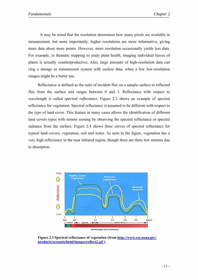
Fundamentals Chapter 2
- 11 -
It may be noted that the resolution determines how many pixels are available in
measurement, but more importantly, higher resolutions are more informative, giving
more data about more points. However, more resolution occasionally yields less data.
For example, in thematic mapping to study plant health, imaging individual leaves of
plants is actually counterproductive. Also, large amounts of high-resolution data can
clog a storage or transmission system with useless data, when a few low-resolution
images might be a better use.
Reflectance is defined as the ratio of incident flux on a sample surface to reflected
flux from the surface and ranges between 0 and 1. Reflectance with respect to
wavelength is called spectral reflectance. Figure 2.3 shows an example of spectral
reflectance for vegetation. Spectral reflectance is assumed to be different with respect to
the type of land cover. This feature in many cases allows the identification of different
land covers types with remote sensing by observing the spectral reflectance or spectral
radiance from the surface. Figure 2.4 shows three curves of spectral reflectance for
typical land covers; vegetation, soil and water. As seen in the figure, vegetation has a
very high reflectance in the near infrared region, though there are three low minima due
to absorption.
Figure 2.3 Spectral reflectance of vegetation (from http://www.csc.noaa.gov/ products/sccoasts/html/images/reflect2.gif ).

Chapter 2 Fundamentals
- 12 -
Figure 2.4 Spectral reflectance of vegetation, soil and water (from http://landsat.usgs.gov/resources/remote_sensing/remote_sensing_applications.php).
Soil has rather higher values for almost all spectral regions. Water has almost no
reflectance in the infrared region. Chlorophyll, contained in a leaf, has strong absorption
at B (0.45 μm) and R (0.67 μm), and high reflectance at NIR (0.7-0.9 μm). This
characteristic reflects in the small peak at G (0.5-0.6 μm), which makes vegetation
green to the human observer. NIR is very useful for vegetation surveys and mapping
because such a steep gradient at 0.7-0.9 μm is produced only by vegetation. Because of
the water content in a leaf, there are two absorption bands at about 1.5 μm and 1.9 μm.
This is also used for surveying vegetation greenness.
2.3 Image correction
2.3.1 Atmospheric correction
Radiation from the Earth's surface undergoes significant interaction with the
atmosphere before it reaches the satellite sensor. This interaction with the atmosphere
can be severe, as in the case of cloud contamination, or minor, as in the case when the
FOV is essentially a clear sky (Schott and Henderson-Sellers, 1984). Regardless of the

Fundamentals Chapter 2
- 13 -
type of analysis that is performed on the remotely sensed data, it is important to
understand the effects of the atmosphere upon the radiance response.
The propagation of electromagnetic radiation through the atmosphere is affected
by two essential processes; absorption and scattering. Absorption occurs when a
fraction of energy passing through the atmosphere is absorbed by some of the
atmospheric constituents and is then re-emitted at different wavelengths. Scattering
occurs when a fraction of energy passing through the atmosphere has its direction
altered through a diffusion of radiation by small particles in the atmosphere. The type
and significance of the scattering depends upon the size of the scattering element
compared to the wavelength of the radiation (Schott and Henderson-Sellers, 1984;
Drury, 1987).
At the shorter wavelengths, attenuation occurs by scattering due to clouds and
other atmospheric constituents, as well as by reflection. The effect of scattering on the
visible wavelengths is significant and must be compensated for when developing
empirical relationships through time. The most significant interaction that thermal
infrared radiation undergoes, as it passes through the atmosphere, is by absorption,
primarily due to ozone and water vapour particles in the atmosphere.
The objective of atmospheric correction is to retrieve the surface reflectance
(that characterizes the surface properties) from remotely sensed imagery by removing
the atmospheric effects. Since atmospheric correction has been shown to significantly
improve the accuracy of image classification, the problem has received considerable
attention from researchers in remote sensing who have devised a number of approaches
to its solution (Crippen, 1987). Most of them are sophisticated approaches (based on
e.g. correlation with ground-based measurements, ground truth methods, in-scene
methods, multiple view angle, multiple altitude techniques, atmospheric propagation
models) but they are computationally challenging and have only been validated on a
very small scale. Simplified approaches (e.g. use of a constant correction factor for each
channel of the dataset) have also been adopted, especially in cases of operational
applications over large areas. Atmospheric correction is beyond the scope of this work
and an overview of methods is given e.g. in Chapter 6 of Schott (1997).
Chapter 2 Fundamentals
- 14 -
2.3.2 Radiometric correction
When the emitted or reflected electromagnetic energy is received by a sensor,
the observed energy does not coincide with the energy emitted or reflected from the
same object observed from a short distance. This is due to several factors which include
the sun's azimuth and elevation, the topography, the atmospheric conditions (e.g. fog or
aerosols) and the sensor response. All such factors influence the observed energy and
radiometric correction is a pre-processing technique that aims at reconstructing the
signal and getting physically-calibrated values. In such context, radiometric errors and
inconsistencies are frequently referred to as noise, which may be defined as any
undesirable spatial or temporal variations in image brightness not associated with
variations in the imaged surface.
There are several others techniques aiming at minimizing the effects of the
above-mentioned factors. One of the most common consists of adjusting the average
and the standard deviation of recorded data. Another one is performing a conversion of
data to a normalized index, e.g. the Normalized Difference Vegetation Index (NDVI),
which will be described in detail in Chapter 3. Other techniques include the least square
method and the histogram matching, i.e. histograms per band and/or per sensor are
calculated and the cumulative histogram with cut-offs at 1% and 99% is then relatively
adjusted to the reference histogram.
2.3.3 Geometric correction
Geometric distortions refer to errors between the actual image coordinates and
the ideal image coordinates, which would be projected theoretically with an ideal sensor
and under ideal conditions. Geometric distortions are classified into internal distortions
that result from the geometry of the sensor (e.g. lens distortion, misarrangement of
detectors, variations of sampling rate), and external distortions that arise from the
position and the attitude of the sensor as well as from the shape of the object, the earth
curvature, and the topographic relief. Geometric correction is therefore achieved by
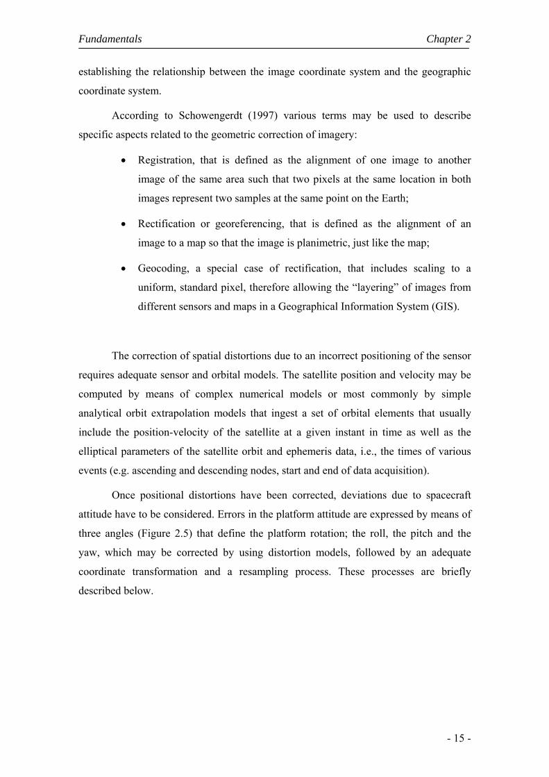
Fundamentals Chapter 2
- 15 -
establishing the relationship between the image coordinate system and the geographic
coordinate system.
According to Schowengerdt (1997) various terms may be used to describe
specific aspects related to the geometric correction of imagery:
• Registration, that is defined as the alignment of one image to another
image of the same area such that two pixels at the same location in both
images represent two samples at the same point on the Earth;
• Rectification or georeferencing, that is defined as the alignment of an
image to a map so that the image is planimetric, just like the map;
• Geocoding, a special case of rectification, that includes scaling to a
uniform, standard pixel, therefore allowing the “layering” of images from
different sensors and maps in a Geographical Information System (GIS).
The correction of spatial distortions due to an incorrect positioning of the sensor
requires adequate sensor and orbital models. The satellite position and velocity may be
computed by means of complex numerical models or most commonly by simple
analytical orbit extrapolation models that ingest a set of orbital elements that usually
include the position-velocity of the satellite at a given instant in time as well as the
elliptical parameters of the satellite orbit and ephemeris data, i.e., the times of various
events (e.g. ascending and descending nodes, start and end of data acquisition).
Once positional distortions have been corrected, deviations due to spacecraft
attitude have to be considered. Errors in the platform attitude are expressed by means of
three angles (Figure 2.5) that define the platform rotation; the roll, the pitch and the
yaw, which may be corrected by using distortion models, followed by an adequate
coordinate transformation and a resampling process. These processes are briefly
described below.
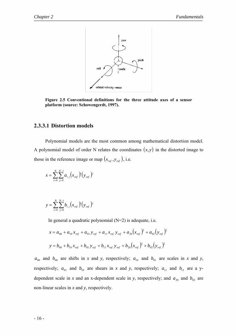
Chapter 2 Fundamentals
- 16 -
Figure 2.5 Conventional definitions for the three attitude axes of a sensor platform (source: Schowengerdt, 1997).
2.3.3.1 Distortion models
Polynomial models are the most common among mathematical distortion model.
A polynomial model of order N relates the coordinates ( )yx, in the distorted image to
those in the reference image or map ( )refref yx , , i.e.
( ) ( )∑∑=
−
=
=N
i
iN
j
jref
irefji yxax
0 0
( ) ( )∑∑=
−
=
=N
i
iN
j
jref
irefji yxby
0 0
In general a quadratic polynomial (N=2) is adequate, i.e.
( ) ( )2022
2011011000 refrefrefrefrefref yaxayxayaxaax +++++=
( ) ( )2022
2011011000 refrefrefrefrefref ybxbyxbybxbby +++++=
00a and 00b are shifts in x and y, respectively; 10a and 01b are scales in x and y,
respectively; 01a and 10b are shears in x and y, respectively; 11a and 11b are a y-
dependent scale in x and an x-dependent scale in y, respectively; and 20a and 02b are
non-linear scales in x and y, respectively.

Fundamentals Chapter 2
- 17 -
In case the image has been processed accurately for systematic distortions, a linear
polynomial usually gives satisfactory results
refref yaxaax 011000 ++=
refref ybxbby 011000 ++=
This linear transformation is known as an affine transformation (Wolf, 1983) and
includes six kinds of distortion, i.e. a translation (or shift) in x, a translation in y, a scale
change in x, a scale change in y, a skew and a rotation.
Coefficients of the polynomial models are usually determined by means of
Ground Control Points (GCPs). Examples of GCPs include natural features (e.g. along
coastlines and rivers), small islands and man-made features (e.g. dams and road
intersections). Once a suitable set of GCPs has been found then coefficients of the
polynomial model may be retrieved by the least-squares technique. However it should
be noted that the goodness-of-fit of the solution does not indicate the validity of the
polynomial model as a model for the physical distortion (Schowengerdt, 1997).
Accordingly, a number of GCPs should be kept for validation but this procedure is
seldom used.
2.3.3.2 Coordinate transformations
Unlike local scale analyses, which treat the Earth as a plane, the precise
determination of the position of points over a broad area must take into account the
actual shape of the Earth that may be approximated by an ellipsoid of revolution or
spheroid, i.e. the geometric figure defined by an ellipse rotated round its minor axis.
The ellipsoid is very important to GIS because heights are measured with respect to the
ellipsoid.
National mapping agencies in different countries around the world use different
ellipsoids, adjusting the lengths of the polar and equatorial radii to get the best fit within
their region of interest (Table 2.2). However recent work based on satellite data has seen
the development of ellipsoids that are used worldwide (e.g. GRS80).
Horizontal and vertical measurements made on the earth are made in the earth's
gravitational field, which can distort those measurements. In fact, the gravity field is

Chapter 2 Fundamentals
- 18 -
dependent on the distribution of the earth mass and some parts of the earth are more
massive than others. If there is a dense mass to one side, “up” will be deflected in the
direction of the mass and “down” will not necessarily be directed toward the centre of
the earth with enough precision for intercontinental distance measurements. Elevation
with respect to mean sea level is therefore measured in respect to the geoid, which is
defined as an equipotential surface derived from the earth's gravity field and the
outward centrifugal force of the earth's rotation. Gravity is accordingly perpendicular to
the geoid at every point. Generally, the geoid is higher over continents and lower over
the oceans (Figure 2.6). Because the geoid is dependent on the irregular distribution of
masses in the earth, the shape of the geoid can not be calculated, only measured.
Table 2.2 Table of Ellipsoids (Adapted from http://ltpwww.gsf.nasa.gov/ IAS/handbook/hamdbook_htmls/chapter1/chapter1.html). Name Date Semi-major
Axis(a) Semi-minor
Axis(b) Use
Airy 1830 6377563.396 6356256.91 Great Britain Bessel 1841 6377397.155 6356078.963 Chile, most parts of
Central Europe, and Indonesia
Clarke 1866 6378206.4 6356583.8 North America and Philippines
Clarke 1880 6378249.145 6356514.87 France, and most of Africa
Everest 1956 6377301.243 6356100.228 India and Nepal Everest 1969 6377295.664 6356094.668 Hayford 1909 6378388 6356911.946 Helmert 1906 6378200 6356818.17 Egypt Hough 6378270 6356794.343
Modified Everest
1948 6377304.063 6356103.039 W. Malaysia and Singapore
Sphere 6370997 6370997 Walbeck 6376896 6355834.847 WGS66 1966 6378145 6356759.769 WGS72 1972 6378135 6356750.52 World wide WGS84 1984 6378137 6356752.31 World wide
The process of converting image coordinates (e.g. lines and columns of pixels)
into positions on Earth requires the adoption of a Coordinate Reference System which
consists of a Coordinate System (i.e. a set of mathematical rules for specifying how
coordinates are to be assigned to points) together with a Datum (EPSG, 2002) that
relates the Coordinate System to the Earth.

Fundamentals Chapter 2
- 19 -
Figure 2.6 Ellipsoid, geoid and topographic surfaces (source: http://www2.uefs.br/geotec/topografia/apostilas/topografia(1).htm).
Among the different Coordinate Systems, map projections are worth mentioning
since they constitute the framework for analysis of remote-sensing imagery
(Schowengerdt, 1997). There is a very wide variety of projection schemes that
constitute trade-offs between different types of distortions (e.g. Gilbert, 1974; Snyder,
1987). Examples of several commonly used map projections are given in Table 2.3 and
an extensive survey on currently used map projections may be found e.g. in EPSG
(2002).
In most maps meridians of longitude and parallels of latitude appear as curved
lines and, to avoid the inconvenience of pinpointing locations on curved reference lines,
cartographers superimpose on the map a rectangular grid consisting of two sets of
straight, parallel lines, uniformly spaced, each set perpendicular to the other. This grid is
designed so that any point on the map can be designated by its latitude and longitude or
by its grid coordinates. Such grids are usually identified by the name of the particular
projection for which they are designed.
The United States National Imagery and Mapping Agency (NIMA) adopted a
special grid for military use throughout the world called the Universal Transverse
Mercator (UTM) grid (USGS, 2001). In this grid, the world is divided into 60 north-
south zones (Figure 2.7), each covering a strip 6° wide in longitude.

Chapter 2 Fundamentals
- 20 -
Figure 2.7 The UTM Zone 29 (source: www.isa.utl.pt/der/Topografia /cartografia2.ppt).
These zones are numbered consecutively beginning with Zone 1, between 180°
and 174° west longitude, and progressing eastward to Zone 60, between 174° and 180°
east longitude. In each zone, coordinates are measured north and east in meters. The
northing values are measured continuously from zero at the Equator, in a northerly
direction. To avoid negative numbers for locations south of the Equator, NIMA's
cartographers assigned the Equator an arbitrary false northing value of 10,000,000
meters. A central meridian through the middle of each 6° zone is assigned an easting
value of 500,000 meters. Grid values to the west (east) of this central meridian are less
(more) than 500,000.
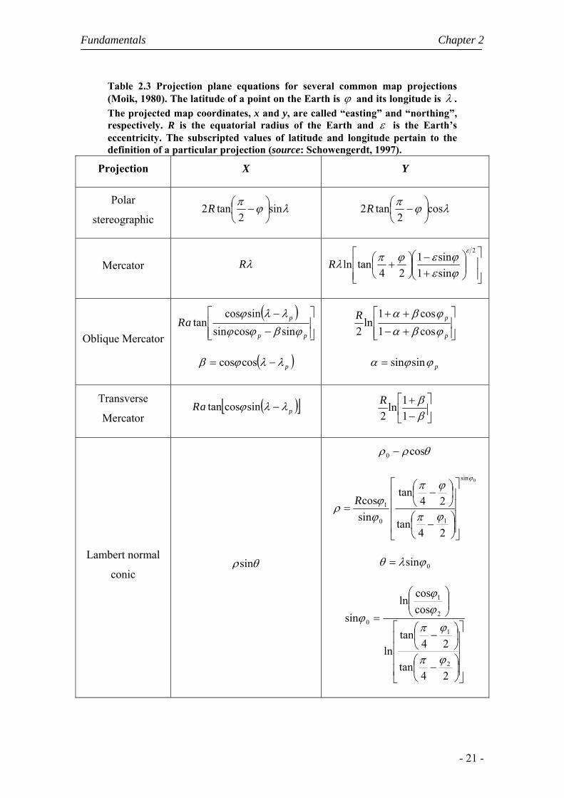
Fundamentals Chapter 2
- 21 -
Table 2.3 Projection plane equations for several common map projections (Moik, 1980). The latitude of a point on the Earth is ϕ and its longitude is λ . The projected map coordinates, x and y, are called “easting” and “northing”, respectively. R is the equatorial radius of the Earth and ε is the Earth’s eccentricity. The subscripted values of latitude and longitude pertain to the definition of a particular projection (source: Schowengerdt, 1997).
Projection X Y
Polar
stereographic λϕπ sin
2tan2 ⎟
⎠⎞
⎜⎝⎛ −R λϕπ cos
2tan2 ⎟
⎠⎞
⎜⎝⎛ −R
Mercator λR ⎥⎥⎦
⎤
⎢⎢⎣
⎡⎟⎟⎠
⎞⎜⎜⎝
⎛+−
⎟⎠⎞
⎜⎝⎛ +
2
sin1sin1
24tanln
ε
ϕεϕεϕπλR
Oblique Mercator
( )⎥⎥⎦
⎤
⎢⎢⎣
⎡
−
−
pp
paRϕβϕϕ
λλϕsincossin
sincostan
( )pλλϕβ −= coscos
⎥⎥⎦
⎤
⎢⎢⎣
⎡
+−
++
p
pRϕβαϕβα
cos1cos1
ln2
pϕϕα sinsin=
Transverse
Mercator ( )[ ]paR λλϕ −sincostan ⎥
⎦
⎤⎢⎣
⎡−+ββ
11ln
2R
Lambert normal
conic θρsin
θρρ cos0 −
0sin
10
1
24tan
24tan
sincos
ϕ
ϕπ
ϕπ
ϕϕ
ρ
⎥⎥⎥⎥
⎦
⎤
⎢⎢⎢⎢
⎣
⎡
⎟⎠⎞
⎜⎝⎛ −
⎟⎠⎞
⎜⎝⎛ −
=R
0sinϕλθ =
⎥⎥⎥⎥
⎦
⎤
⎢⎢⎢⎢
⎣
⎡
⎟⎠⎞
⎜⎝⎛ −
⎟⎠⎞
⎜⎝⎛ −
⎟⎟⎠
⎞⎜⎜⎝
⎛
=
24tan
24tan
ln
coscosln
sin
2
1
2
1
0
ϕπ
ϕπϕϕ
ϕ
Chapter 2 Fundamentals
- 22 -
2.4 Resampling
Once the coordinate transformation from ( )refref y,x to ( )y,x has been
determined then the transformation is applied by stepping through the reference
coordinates and computing the corresponding distorted coordinates ( )y,x . Computed
values of ( )y,x will not usually match the values of the pixels of the image and
therefore there is the need to proceed to the interpolation of the “new” pixels between
the existing pixels in the image. This procedure is usually referred to as resampling.
There are several interpolation schemes to compute the value of a resampled
pixel; these include:
• the nearest neighbour method;
• the bilinear interpolation method;
• the cubic convolution method.
A) Nearest neighbour method
In this method, also called zero-order interpolation, each new pixel at ( )refref y,x
gets the value of the original pixel whose location ( )y,x is the nearest to it.
The nearest neighbour method (e.g. Cracknell, 1998) does not require any
computations and therefore has the advantage of being very fast to use. Besides, it does
not lead to any loss of information due to smoothing and no new values are introduced
in the statistical distribution. However, the “round-off” property that is inherent to the
method may cause geometric discontinuities of the order of ± ½ pixel, which may be the
cause of spurious effects (e.g. omission or repetition of pixels).
B) Bilinear interpolation method
In this method, also called first-order interpolation, the estimate of the value of the
output pixel located at ( )refref y,x is based on the values of the four surrounding input
pixels located in the original space ( )yx, . The method consists in performing two linear
Fundamentals Chapter 2
- 23 -
interpolations, one along the lines (x direction) that creates a new resampled column (y
direction), the final value at ( )y,x being again obtained by linear interpolation.
Bilinear resampling is computationally much more expensive and produces a
much smoother interpolating surface than the nearest-neighbour method. This
smoothing effect is especially conspicuous in sharp boundaries that become blurred
after bilinear interpolation.
C) Cubic convolution method
The cubic convolution method, also called bicubic or third-order interpolation,
avoids the excessive smoothing of bilinear resampling. The method involves fitting
third-degree polynomials using the 16 nearest pixels located in the original space ( )y,x
that surround the output pixel ( )refref y,x . However, unlike bilinear resampling, the
method may create values outside the original range.
In the case of thematic maps (e.g. land cover maps) resampling is usually
performed by using either the already described nearest neighbour method or the so-
called majority rule, where the output pixel ( )refref y,x is assigned to the most frequent
class as observed in a given window of pixels in the original space ( )y,x . The majority
rule will be described in detail in section 3.2.3.

Chapter 2 Fundamentals
- 24 -
2.5 The SPOT and the NOAA systems
2.5.1 The SPOT Program
The SPOT (Satellite Pour l’Observation de la Terre) program consists of a series
of optical remote sensing satellites with the primary mission of obtaining Earth imagery
for land use, agriculture, forestry, geology, cartography, regional planning, water
resources and GIS applications. The program is committed to commercial remote
sensing on an international scale and has established a global network of control
centres, receiving stations, processing centres and data distributors. SPOT satellites are
operated by the French Space Agency, the Centre National d'Etudes Spatiales (CNES).
SPOT 1 was first launched in February, 1986, with successors following every
three or four years. SPOT 2 was launched in January, 1990 and SPOT 3 was launched
in September 1993; SPOT 4 was launched on March 1998 and SOPT 5 followed on
May 2002. The orbit of SPOT 1 was lowered in 2003 and the satellite will gradually
loose its altitude and break up on the atmosphere. The recorders on-board SPOT 2 are
not working but the satellite is still able to provide imagery. SPOT 3 is not working
anymore but SPOT 4 and SPOT 5 are fully functional.
All satellites are in sun-synchronous, near-polar orbits at altitudes of about 830
km above the Earth, and have orbit repetitions of 26 days. The SPOT system provides
global coverage between the latitudes of 87ºN and 87ºS. The loads of SPOT 1, SPOT 2
and SPOT 3 were the same, each satellite carrying two identical High Resolution
Visible (HRV) imaging instruments. As shown in Table 2.4, the HRV instrument is able
to operate in two modes; the panchromatic (PAN) mode and the multispectral (MS)
mode. In PAN, imaging is performed in a single spectral band that covers the visible
part of the electromagnetic spectrum. In MS, imaging is performed in three spectral
bands, green, red and NIR.

Fundamentals Chapter 2
- 25 -
Table 2.4 HRV Spectral Bands. (from http://www.spotimage.fr/html/ _167_224_230_.php).
Mode Band Wavelength (µm) Resolution (m)
Multispectral XS1 0.50 - 0.59 (Green) 20
Multispectral XS2 0.61 - 0.68 (Red) 20
multispectral XS3 0.79 - 0.89 (Near IR) 20
Panchromatic P 0.51 - 0.73 (Visible) 10
In the case of SPOT 4 (Figure 2.8) the two imaging instruments were upgraded,
becoming the High Resolution Visible and Infrared (HRVIR) instrument. As shown in
Table 2.5 the HRVIR is similar to the HRV, except that HRVIR has an additional SWIR
band, and the wavelength bandwidth of the panchromatic mode is narrower than that for
HRV.
Figure 2.8 Picture of the satellite SPOT 4. (from http://medias.obs-mip.fr/www/Reseau/Lettre/11/en/systemes/vegetation.html).
In the field of environment and agriculture, the sensitivity of the SWIR band to
variations in canopy or soil water content produces a high contrast between soil and
vegetation reflectances, leading to an easier detection of variations in the canopy
structure. The SWIR band is therefore especially interesting for the discrimination of
wet areas, the identification of water stress in plants, the classification of some crops
and vegetation areas. In particular, the SWIR enables to obtain a better characterisation
of arid and semi-arid areas and reveals to be also useful to study forest areas. In

Chapter 2 Fundamentals
- 26 -
particular, it provides increased precision for the mapping of forests types, with special
interest for areas poorly mapped (e.g. tropical environment), as well as for the
estimation of cover rate and the relative humidity of plant communities.
Table 2.5 HRVIR Spectral Bands (from http://www.spotimage.fr/html/ _167_224_230_.php).
Mode Band Wavelength (µm) Resolution (m)
Multispectral XI1 0.50 - 0.59 (Green) 20
Multispectral XI2 0.61 - 0.68 (Red) 20
Multispectral XI3 0.79 - 0.89 (Near IR) 20
Multispectral XI4 1.53 - 1.75 (SWIR) 20
Monospectral M 0.61 - 0.68 (Red) 10
As shown in Figure 2.9, the two HRV (or HRVIR) sensors operate in a cross-track
direction. The position of each HRV (or HRVIR) entrance mirror can be commanded by
ground control to observe a region of interest not necessarily vertically beneath the
satellite. Thus, each HRV (or HRVIR) offers an oblique viewing capability, the viewing
angle being adjustable through ±27º relative to the vertical. This off-nadir viewing
enables the acquisition of stereoscopic imagery and provides a short revisit interval of 1
to 3 days (Figure 2.10). Moreover, due to the parallax thus created, the oblique viewing
capacity of SPOT makes it possible to produce “stereopairs” by combining two images
of the same area acquired on different dates and at different angles, due to the parallax
thus created.

Fundamentals Chapter 2
- 27 -
Figure 2.9 The cross-track direction operating mode of the two HRV sensors. (from http://www.spotimage.fr/html/_167_224_230_.php)
Figure 2.10 Repeated observation by SPOT. (from http://www.spotimage.fr/ html/_167_224_230_.php)
Both the HRV and the HRVIR instruments were constructed with multilinear
array detectors. In particular, the HRVIR instrument was designed to acquire,
instantaneously, one complete line of pixels at a time covering the entire field of view.
This is attained using a charged-couple device (CCD) linear array. The CCD linear
arrays operate in the so-called "push-broom" mode (Figure 2.11). A wide-angle
telescope forms an instantaneous image of adjacent "ground patch areas" on a row of
detectors in the instrument's focal plane. Column-wise scanning is a direct result of the

Chapter 2 Fundamentals
- 28 -
satellite's motion along its orbit. The signals generated by the detectors (photodiodes)
are read out sequentially at a predetermined clock rate. Thus, although the linear arrays
do not "scan" in the line-wise direction to gather light, the detectors are scanned
electronically to generate the output signal. The telescope has a field of view of 4°,
corresponding to 60 km on the ground covered instantaneously by a line of 6000
detectors. Each HRVIR is thus said to offer a "strip width" of 60 km (Figure 2.12).
Figure 2.11 The push broom principle (http://spot4.cnes.fr/spot4_gb/ index.htm).
Figure 2.12 SPOT’s Field of view. (from http://spot5.cnes.fr/gb/satellite/ 42.htm)
As a complement to the two HRVIR instruments, SPOT 4 takes on board the
VEGETATION instrument that is part of the so-called VEGETATION system.

Fundamentals Chapter 2
- 29 -
The VEGETATION system is the result of a co-operation between the European
Union, France, Sweden, Belgium and Italy. It aims at ensuring a regional and global
continuous monitoring of the continental biosphere and of crops. It observes the Earth at
a resolution of 1.15 km, quite invariable in the swath width of nearly 2250 km (Figure
2.13). This gives almost daily access to any point on the earth surface. Taking into
account the measurements which have to be discarded due to cloud coverage or bad
atmospheric conditions, this feature minimises the probability to get one useful
measurement per ten-day periods, the multitemporal spatial resolution being of about 1
km. These characteristics allow the observation and study of seasonal evolutions in the
biosphere and its processes. Moreover, SPOT enables to lead these studies and
observations in a multi-scale context, as the spectral bands and geometrical references
of the VEGETATION instrument are the same for the two HRVIR instruments, the
three instruments being inter-calibrated.
Figure 2.13 The VEGETATION field of view. (from http://spot5.cnes.fr/gb/ satellite/42.htm)
The new SPOT 5 satellite is designed to ensure SPOT data users with continuity
of service, enhanced image quality and improved services. Derived from the HRVIR
instruments on SPOT 4, the two new HRG instruments offer higher resolution: 2.5
metres to 5 metres in panchromatic mode and 10 metres in multispectral mode. Imagery
at a resolution of 2.5 metres is generated using a new sampling concept dubbed
"Supermode". SPOT 5 features a new HRS imaging instrument operating in
panchromatic mode. SPOT 5 is also carrying the recurrent VEGETATION 2
instrument. Tables 2.6 and 2.7 respectively show the orbit characteristics for SPOT 5
and the VEGETATION characteristics, for the four multi-spectral bands.
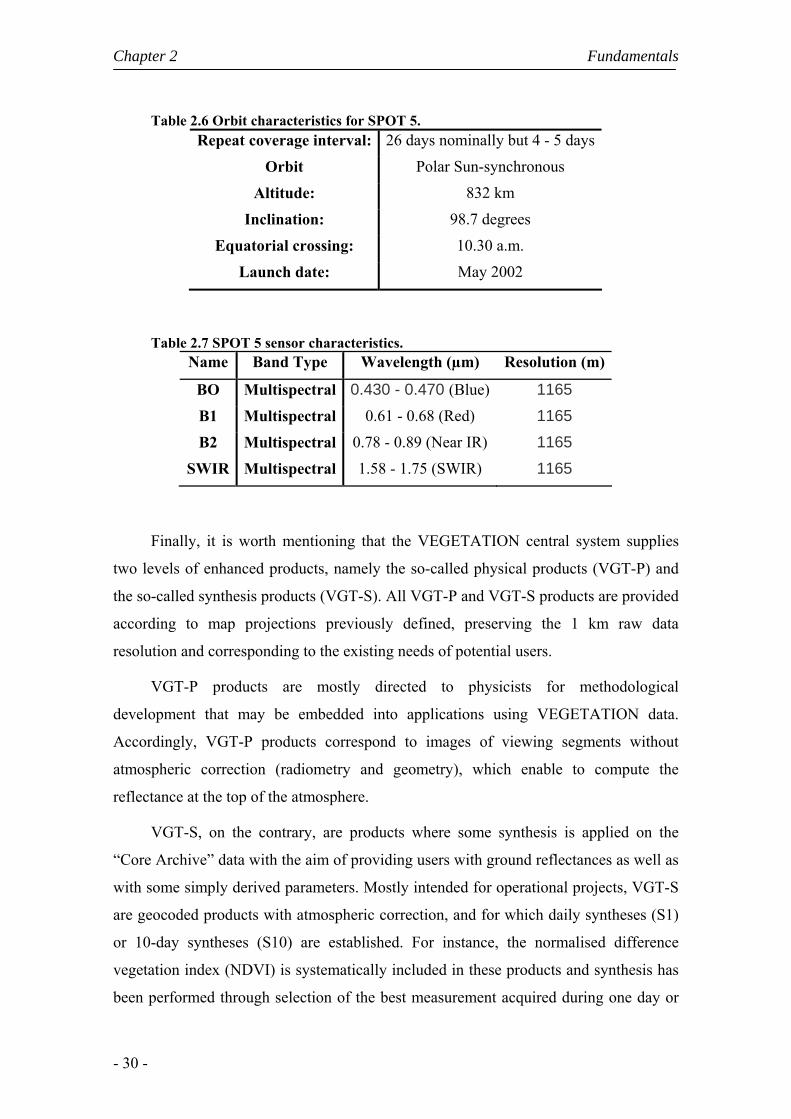
Chapter 2 Fundamentals
- 30 -
Table 2.6 Orbit characteristics for SPOT 5.
Repeat coverage interval: 26 days nominally but 4 - 5 days
Orbit Polar Sun-synchronous
Altitude: 832 km
Inclination: 98.7 degrees
Equatorial crossing: 10.30 a.m.
Launch date: May 2002
Table 2.7 SPOT 5 sensor characteristics. Name Band Type Wavelength (µm) Resolution (m)
BO Multispectral 0.430 - 0.470 (Blue) 1165
B1 Multispectral 0.61 - 0.68 (Red) 1165
B2 Multispectral 0.78 - 0.89 (Near IR) 1165
SWIR Multispectral 1.58 - 1.75 (SWIR) 1165
Finally, it is worth mentioning that the VEGETATION central system supplies
two levels of enhanced products, namely the so-called physical products (VGT-P) and
the so-called synthesis products (VGT-S). All VGT-P and VGT-S products are provided
according to map projections previously defined, preserving the 1 km raw data
resolution and corresponding to the existing needs of potential users.
VGT-P products are mostly directed to physicists for methodological
development that may be embedded into applications using VEGETATION data.
Accordingly, VGT-P products correspond to images of viewing segments without
atmospheric correction (radiometry and geometry), which enable to compute the
reflectance at the top of the atmosphere.
VGT-S, on the contrary, are products where some synthesis is applied on the
“Core Archive” data with the aim of providing users with ground reflectances as well as
with some simply derived parameters. Mostly intended for operational projects, VGT-S
are geocoded products with atmospheric correction, and for which daily syntheses (S1)
or 10-day syntheses (S10) are established. For instance, the normalised difference
vegetation index (NDVI) is systematically included in these products and synthesis has
been performed through selection of the best measurement acquired during one day or

Fundamentals Chapter 2
- 31 -
one decade. As described in the next chapter, such selection is based on the Maximum
Value Composite (MVC) technique where the retained measurement simply
corresponds to the highest NDVI value computed on top of atmosphere reflectances.
2.5.2 The NOAA series
Starting with TIROS-1 in 1960, the first and the second generations of the US
National Oceanic and Atmospheric Administration (NOAA) polar orbiting satellites
reached the third generation of meteorological satellites with the launch of TIROS-N in
1978. The first generation was the TIROS series (1960-1965), while the second
generation was ITOS series (1970-1976). TIROS-N has been followed by NOAA-6
through NOAA-18 (Table 2.8).
Table 2.8 General time coverage by satellite. (from http://www.ngdc.noaa.gov/ stp/NOAA/noaa_poes.html)
TIROS-N 1978 - 1981
NOAA-6 1979 - 1986
NOAA-7 1981 - 1985
NOAA-8 1983 - 1985
NOAA-10 1986 - 1991
NOAA-12 1991 - 2002
NOAA-14 1994 - 2004
NOAA-15 1998 - present
NOAA-16 2001 - present
NOAA-17 2002 - present
NOAA-18 2005 - present
NOAA satellites operate at an altitude of approximately 850 km with slight
inclined orbits of approximately 98.8º and an orbital period of about 101.5 min (i.e. 14.2
orbits per day). Since the number of daily orbits is not an integer, the sub-orbital tracks
do not repeat on a daily basis, although the Local Solar Time (LST) of the satellite’s
passage is essentially unchanged for any latitude. However, the satellite’s orbit drifts
over time, causing a systematic change of illumination conditions and local time of

Chapter 2 Fundamentals
- 32 -
observation, which is the major source of non-uniformity in multi-annual satellite time
series.
NOAA has two types of satellites operating in complementary orbits, one crossing
the Equator around 0730 and 1930 LST and the other one around 0230 and 1430 LST.
For reasons of convention, even satellites cover the “morning orbit” (0730), while the
odd ones cover the “afternoon orbit” (1430). Table 2.9 shows the orbit characteristics
for several NOAA satellites covering the “afternoon orbit”.
Table 2.9 NOAA Satellites Orbital Characteristics. (Adapted from http://www.crisp.nus.edu.sg/~research/tutorial/noaa.htm)
NOAA-12 NOAA-14 NOAA-16 NOAA-18 Launch date 14 May 1991 30 Dec 1994 21 Sep 2000 20 May
2005
Date operations began 17 Sep 1991 10 Apr 1995 20 Mar 2001 30 Oct 2005
Orbit inclination 98.5 99.1 98.8 98.8
Mean altitude (km) 808 847 851 833
Equator crossing time (A: Northbound, B: Southbound)
16:49A, 04:49D
17:52A, 05:52D
13:54A, 01:54D
Period (min.) 101.2 101.9 102.1 101.35
One of the main instruments carried on-board the NOAA satellites is the
Advanced Very High Resolution Radiometer (AVHRR) with a 1.1 km instantaneous
field of view (IFOV) for a swath of 2,800 km in the visible and infrared wavelength
regions. The earlier AVHRR instrument on-board NOAA 9, 10, 11, 12 had 5 bands,
respectively in the visible (band 1), NIR (band 2), MIR (band 3) and TIR (bands 4, 5)
regions. Starting from NOAA-14, the newer AVHRR instrument (AVHRR/2) has an
extra band in the SWIR. This band shares the same transmission channel with the
MWIR band which is designated Band 3A, while the SWIR band is Band 3B. Only one
of the 3A or 3B bands is activated at any instant. Table 2.10 presents the AVHRR
Sensor Characteristics of each band.

Fundamentals Chapter 2
- 33 -
Table 2.10 AVHRR Sensor characteristics. (from http://www.crisp.nus. edu.sg/~research/tutorial/noaa.htm)
Band Wavelength (µm)
Applications
Visible 1 0.58-0.68 cloud, snow and ice monitoring
Near IR 2 0.725-1.10 water, vegetation and agriculture surveys
Short Wave IR 3A 1.58-1.64 snow, ice and cloud discrimination
Medium Wave IR
3B 3.55-3.93 sea surface temperature, volcano, forest fire activity
Thermal IR 4 10.3-11.3 sea surface temperature, soil moisture
Thermal IR 5 11.3-12.5 sea surface temperature, soil moisture
There is another important sensor on-board NOAA satellites, namely the TIROS
Operational Vertical Sounder (TOVS) which consists of three units; the High
Resolution Infrared Sounder; model 2 (HIRS/2) with 20 km IFOV, for a 2,200 km
swath, the Stratospheric Sounding Unit (SSU) with 147 km IFOV, for a 736 km swath
and the Microwave Sounding Unit (MSU) with 110 km IFOV, for a 2,347 km swath.
AVHRR data are acquired in three formats: High Resolution Picture Transmission
(HRPT), Local Area Coverage (LAC) and Global Area Coverage (GAC). HRPT data
are full resolution image data which are transmitted to a local ground station as they are
being collected. Many weather stations around the world operate ground stations that
routinely receive real-time HRPT data. LAC data are also full resolution, but they are
recorded in an on-board tape for subsequent transmission during a station overpass.
Since the on-board tape facility is limited, only a number of scenes are archived. GAC
data are subsampled on-board to about 4-km pixel separation at nadir and provide daily
global coverage. GAC data are also recorded on tape and then transmitted to a ground
station. LAC and GAC data are available from NOAA's Satellite Active Archive (SAA)
through the world-wide web (http://www.saa.noaa.gov).


3. BASIC DATA AND PRE-PROCESSING
3.1 Vegetation Indices
3.1.1 Introduction
Changes in vegetation have a strong impact on human activities around the globe.
For instance, over the last 50 years deforestation in South America has left vast areas
uncultivated and has destroyed many species. One of the major advantages of remote
sensing data is its capability of detecting and quantifying green vegetation. Satellite data
may for instance be used to detect vegetative changes from one growing season to the
next, from year to year, or from decade to decade.
The principle behind the detection of green vegetation is connected with the use
of blue and red radiation as energy sources for actively photosynthesizing plants. On the
other hand, and as already pointed out in the previous chapter, near-infrared radiation is
highly reflected by vegetation (Figure 3.1). Several algorithms have been developed
which combine the measured radiances reflected by land surface in different spectral
bands of the atmospheric window in order to obtain the so-called "Vegetation Indices"
(VIs), that are able to discriminate green vegetation.
Figure 3.1 Reflectance from different wavelengths and different surfaces.

Chapter 3 Basic Data and Pre-Processing
- 36 -
A VI may therefore be used to quantify concentrations of green leaf vegetation
and identify those places where vegetation is either green or under stress due to the
absence of water. In fact, several authors have shown that VIs are well correlated with
vegetation amount, unstressed vegetation and photosynthetic capacity (Tucker, 1979;
Sellers et al., 1992) as well as with other parameters, such as the Leaf Area Index (LAI)
and the Fraction of Absorbed Photosynthetically Active Radiation (FAPAR), that
quantify biomass and physiological functioning. For instance, LAI may be derived
based on a regression model derived from a vegetation index and ground measurements
of the considered type of vegetation (Holben et al. 1980; Li et al. 1993; Chen and
Cihlar, 1996).
Other models based on indices have been designed to both detect sparse green
vegetation and minimize the effects of soil background brightness, topographical
distortion and atmospheric “noise”.
In general terms, VIs may be divided into two main groups, referred to as
Empirical Vegetation Indices and Optimised Vegetation Indices. The most commonly
used VI, the so-called Normalized Difference Vegetation Index (NDVI), belongs to the
first group. NDVI was introduced by Rouse et al. (1974) and is defined as:
rednir
rednirNDVIρρρρ
+−
=
NDVI ranges between –1.0 and +1.0 and assumes positive values for areas with
vegetation. Very low values of NDVI (0.1 and below) are characteristic of barren areas
of rock, sand, or snow. Moderate values are associated to shrub and grassland (0.2 to
0.3), while high values indicate temperate and tropical rainforests (0.6 to 0.8). As
already pointed out, healthy green leaves commonly have larger reflectances in the near
infrared than in the visible range. As the leaves come under water stress, become
diseased or die back, they become more yellow and reflect significantly less in the near
infrared range. Additionally, unhealthy or sparse vegetation reflects more visible light
and less near-infrared light (Figure 3.1).
Basic Data and Pre-Processing Chapter 3
- 37 -
Clouds, water, and snow have larger reflectances in the visible than in the near
infrared whereas the difference is almost zero for rock and bare soil. However, actual
vegetation status cannot be observed under cloudy sky conditions. Tropical areas, for
instance, are often covered with clouds, becoming very hard to obtain cloud-free data at
once for entire areas. In order to overcome this difficulty, NDVI data with little
influence of cloud are usually produced by extracting the maximum value of NDVI
from data series covering a long enough period, e.g. one month at each grid point.
However, values of NDVI may still be low when cloud or ice covers the vegetation for
the whole considered period. In the case of water bodies, such class of pixels is usually
masked by assigning a conventional value (e.g. zero).
3.1.2 Performance and limitations of empirical vegetation indices
Vegetation indices were introduced over more than 25 years ago as a simple
remote sensing tool. Still largely used today, their usage requires however a good
understanding of their respective advantages and drawbacks when analysing remote
sensing data. For instance, and in what respects to NDVI, it is important to understand
that NDVI holds only a fraction of the information available in the original spectral
reflectance data. Users of NDVI have in fact tended to estimate a large number of
vegetation properties (e.g., LAI, FAPAR, chlorophyll concentration in leaves, plant
productivity, fractional vegetation cover and accumulated rainfall). However, if
correctly used, an appropriate VI may be converted into a useful product and is also an
important tool to estimate the likelihood that vegetation is actively growing at a
particular location. The correct usage and interpretation of an index generally depends
on how it was designed, but there is no single and definite meaning.
It is worth stressing that NDVI turns out to be sensitive to a number of perturbing
factors induced by clouds, atmospheric conditions and soil type. NDVI is also sensitive
to anisotropic and spectral effects. Accordingly, in the case of quantitative applications
that require a given level of accuracy, the perturbing factors may lead to errors or
uncertainties of the same order of magnitude of the quantities to be evaluated. In such
cases, special care must be taken to remove perturbations from the data and this may
require extensive processing based on ancillary data and other sources of information.

Chapter 3 Basic Data and Pre-Processing
- 38 -
Optimized vegetation indices represent an alternative to the use of empirical VIs.
Such indices are ‘optimized’ in the sense that they are specifically designed to
physically estimate a given geophysical or biological variable. During the last decades,
a new generation of spectral indices has been developed in order to estimate a specific
environmental variable on the basis of data from a specific instrument. The rationale
behind the design of optimized vegetation indices is described e.g. in Verstraete and
Pinty (1996) and Govaerts et al. (1999). This approach has been developed and applied
in the context of a wide range of sensors, including SeaWiFS, VEGETATION, MIRS
and MERIS (Gobron et al.; 2000; 2001; 2002). The design of optimized vegetation
indices is based on exploiting combinations of spectral bands that have a maximal
sensitivity to the presence and to changes in the properties of healthy green vegetation.
In addition indices should have a minimal sensitivity to atmospheric scattering and
absorption effects, to soil color and brightness changes, and to temporal and spatial
variations in the geometry of illumination and observation.
Besides the simplicity and low computational cost, NDVI presents the advantage
of the availability and continuity of the datasets (25 years of AVHRR NDVI), which
represents an invaluable feature for climatic studies. In fact, when the aim is to study the
status of vegetation due to climate variability, namely droughts and extreme events (e.g.
heat waves), results based on the analysis of NDVI time series have brought some
satisfactory insights. An example is shown in Figures 3.2 and 3.3 that present the results
obtained during the extreme heat wave that has stricken Europe in August 2003. Results
shown in Figure 3.2 were obtained using NDVI data as obtained from the
VEGETATION instrument on board SPOT4, whereas those in Figure 3.3 are based on
FAPAR as derived from the MERIS instrument on board ENVISAT platform. It may be
noted that FAPAR is a physically-based quantity, defined as the fraction of
photosynthetically active radiation (400 -700 nm) absorbed by vegetation canopies.
Figure 3.2 presents monthly anomalies of NDVI during August 2003 and the anomaly
was calculated with respect to a base period as obtained for the years 1999-2004
(excluding 2003). Negative (positive) anomalies correspond to lower (higher) than
average NDVI. Figure 3.3 presents monthly FAPAR anomalies for August 2003 over
Europe (Gobron et al., 2005). The anomaly is calculated with respect to a base period
taken over the years of 1998 to 2002. In both cases the base period does not include the
year of 2003 and it may be noted that anomaly fields of NDVI and FAPAR are
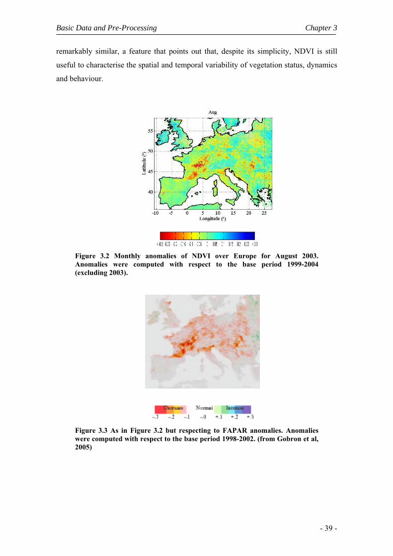
Basic Data and Pre-Processing Chapter 3
- 39 -
remarkably similar, a feature that points out that, despite its simplicity, NDVI is still
useful to characterise the spatial and temporal variability of vegetation status, dynamics
and behaviour.
Figure 3.2 Monthly anomalies of NDVI over Europe for August 2003. Anomalies were computed with respect to the base period 1999-2004 (excluding 2003).
Figure 3.3 As in Figure 3.2 but respecting to FAPAR anomalies. Anomalies were computed with respect to the base period 1998-2002. (from Gobron et al, 2005)

Chapter 3 Basic Data and Pre-Processing
- 40 -
In the present work we will use, for climatological purposes, two datasets of
NDVI, respectively derived from VEGETATION/SPOT and NOAA/AVHRR. The two
databases will be described in the following two sections.
3.1.3 NDVI from AVHRR/NOAA
The NDVI database as derived from AVHRR/NOAA has been widely used in
studying vegetation and ecosystems, especially in semi-arid environments where
vegetation cover is less than 30% (Huete and Tucker, 1991; Karnieli et al., 1996). In
particular, NOAA-AVHRR derived NDVI and other related indices have been
successfully used to identify and monitor areas affected by drought at the regional and
the local scales (Malingreau, 1986; Bayarjargal et al., 2006, Vicente-Serrano, 2007).
Relationships have also been found between NDVI and other vegetation indicators such
as Leaf Area Index (LAI) (Myneni and Williams, 1994) and green biomass production,
as well as with rainfall or soil moisture in semi-arid environments (Schmidt and
Karnieli, 2000).
In our study we have used monthly values of NDVI and of channel 4 brightness
temperature, at 8-km resolution, from the Advanced Very High Resolution Radiometers
(AVHRR), as provided by the Global Inventory Monitoring and Modelling System
(GIMMS) group (Pinzon et al., 2005; Tucker et al., 2005). The GIMMS NDVI datasets
were generated with the aim of providing a 22-year satellite record (1982-2003) of
monthly changes in terrestrial vegetation. Such long-term series of NDVI may be used
in climate and biogeochemical models to calculate photosynthesis, the exchange of CO2
between the atmosphere and the land surface, the land-surface evapotranspiration and
the absorption and release of energy by the land surface (Tucker et al., 2005).
It is worth emphasizing that several factors have to be taken into account when
building up a long-term time series of NDVI. For instance, band calibrations have
changed substantially during considered 22 years (five NOAA/AVHRR instruments).
Natural variability in atmospheric aerosols and column water vapour has also affected
the NDVI record. Over the acquisition period there were two major volcanic eruptions,
El Chichon in May-July 1982 and Mount Pinatubo in July-September 1991, which
injected large quantities of aerosols into the Earth’s stratosphere. These aerosols, along

Basic Data and Pre-Processing Chapter 3
- 41 -
with smoke from biomass burning and dust from soil erosion and other sources, may
have introduced significant variability in the AVHRR/NDVI dataset.
The pre-processing of satellite data involved cloud screening and calibration for
sensor degradation and inter-sensor variations (Los, 1998). Cloud screening was
provided by a channel 5 thermal mask of 0ºC for all continents except Africa, where a
cloud mask of 10ºC was used. In addition, the bimonthly composites significantly
reduced cloud contamination. The data from April 1982 to December 1984 and from
June 1991 to December 1993 were corrected to remove the effects of stratospheric
aerosol from El Chichon and Mount Pinatubo eruptions (Tanré et al., 1992), as well as
NOAA-9 descending node data from September 1994 to January 1995 (Los, 1998). In
fact, in 1992, NOAA-13 has failed to achieve orbit and NOAA-11 continued to supply
global afternoon/early morning AVHRR data. From September 1994, the GIMMS
group began to use NOAA-9 descending node AVHRR data for the global NDVI data
set and continued using these data until NOAA-14 became operational in late January
1995. This feature constitutes a fundamental difference between the GIMMS NDVI and
other AVHRR NDVI datasets, such as the Pathfinder AVHRR Land (PAL) data and the
Global Vegetation Index (GVI) datasets. In the case of GIMMS the gap of data from
September 1994 to January 1995 was filled using the NOAA-9 data while the other
datasets present missing data (Pettorelli at al., 2005).
NDVI is also sensitive to the periodic variations in solar illumination angle and to
sensor viewing angles induced by the NOAA orbits. The polar, sun-synchronous orbits
of the NOAA series allow daily coverage of each point on earth, although at time-
varying viewing and illumination geometry. The GIMMS NDVI dataset has a satellite
overpass time drift correction that largely eliminates the variation of NDVI due to
changes in solar zenith angle.
The GIMMS group uses the so-called Empirical Mode Decomposition (EMD) to
identify and remove parts of the NDVI signal that are most related to the satellite drift
(Pinzon 2002; Pinzon et al. 2004). The EMD is empirical, intuitive, direct, a posteriori,
and adaptive, with the decomposition functions based on and derived from the data
(Huang et al. 1998; Huang et al. 1999). Pinzon et al. (2001) showed that EMD was
applicable to NDVI time series from the AVHRR sensor to isolate orbital drift effects
from the NDVI signal. Further details on the quality of the AVHRR dataset may be
found in Kaufmann et al. (2000) and Zhou et al. (2001).

Chapter 3 Basic Data and Pre-Processing
- 42 -
The GIMMS data set is originally defined on an Alberts Conical Equal-area
projection, using the Clarke ellipsoid. Data used in our study respects to a window
covering the Eurasian and the North Atlantic regions, from 30º W to 60º E and from 30º
to 75º N, over the 21-year long period, from 1982 to 2002. This dataset will be used in
Chapters 4 and 5 and it is worth mentioning that NDVI values were re-projected to
geographic coordinates, using a nearest neighbour scheme (Chapter 2).
3.1.4 NDVI data fromVEGETATION/SPOT
As pointed out in Chapter 2, VEGETATION on board SPOT 4 and SPOT 5 is an
optical multi-spectral instrument that performs an almost complete cover of the Earth
surface in four spectral bands (Hagolle et al., 2005), on a daily basis. NDVI data were
extracted from the S10 products of the VITO database (http://free.vgt.vito.be), which
are supplied at the resolution of 0.008928º (i.e., about 1 km2 resolution at equator) in
geographic coordinates (Lat/Lon), using the WGS84 ellipsoid It may be noted that
supplied values of NDVI were derived from atmospherically corrected and
geometrically calibrated data and that we have restricted to the period from September
1998 to July 2006 over the region extending from 37º N to 42º N and from 9º W to 6º E.
NDVI fields are given on a 10-day basis as derived using the Maximum Value
Composite method (MVC, Holben, 1986), which simply consists in selecting, for each
pixel, the date of maximum NDVI among 10 consecutive daily images. Despite some
problems, time series of MVC-NDVI composites have proven to be a source of valuable
information for monitoring surface vegetation dynamics at the global and the regional
scales (Zhou et al., 2001; Lucht et al., 2002; Nemani et al., 2003). Remaining problems
are related with contamination by clouds, shadows and snow, with sun/view directional
dependence of the spectral response as well as with the dependence of phenological
changes both on time of observation and on geographical location.
In order to create a consistent dataset of vegetation phenology, the yearly time-
series of VGT-NDVI were analysed and corrected, following the method proposed by
Stockli and Vidale (2004) that has been successfully applied to the Pathfinder NDVI
data in order to create a continuous European vegetation phenology dataset of 10-day
temporal and 0.1º spatial resolution. The approach involves two steps in the spatio-
temporal interpolation process; i) a replacement of no-data values in the dataset by

Basic Data and Pre-Processing Chapter 3
- 43 -
spatial interpolation and ii) an adjustment of the NDVI time-series by using a temporal
interpolation procedure.
The methodology relies on the application of an adjustment algorithm based on a
weighted second-order Fourier analysis of the data, as previously described by Sellers et
al. (1996) and Los (1998). This approach uses different correction procedures for the
growing and the non-growing season and therefore requires a precise definition of the
growing season, which in Portugal usually starts with the hydrological year, i.e. year N
starts in the second decade of August of year N-1 and ends in the first decade of August
of year N).
The correction method was applied to VGT-NDVI 10-day composites with 1 km
spatial resolution for the period from September of 1998 to July 2006. Figure 3.4 shows
four representative examples of corrected (red line) and non-corrected (green dots)
monthly time-series of NDVI for different land cover types.
Figure 3.4 Monthly time-series of NDVI for the period 1999–2006 and respecting to four different land cover types; an arable land pixel located in South Alentejo (left top panel), an arable land pixel located in North Alentejo (right top panel), a coniferous forest pixel (left bottom panel) and a broad-leaved forest pixel (right bottom panel). Green dots and the solid curve respectively represent the time series of corrected and non-corrected NDVI monthly values.
With the exception of the coniferous type, the years of 1999 and 2005 are
conspicuous in the time series because of the low photosynthetic activity. This is
especially apparent in the case of the pixels associated to arable land (Figure 3.4, top
panels). In particular, in the case of the arable land pixel located in South Alentejo (top

Chapter 3 Basic Data and Pre-Processing
- 44 -
left panel) the years of 1999 and 2005 reveal marked signs of stress in the vegetation,
which presents shorter vegetation cycles together with lower values of NDVI. In the
case of forest pixels (low panels), the coniferous forest, as expected, presents a high
photosynthetic activity along the year (high NDVI values) together with low interannual
variability, while the broad-leaved type presents a pronounced year cycle of NDVI.
Figure 3.5 shows the results that were obtained when applying to non-corrected
(left panel) and to corrected (right panel) NDVI pixels a technique aiming to detect
years affected by drought conditions. The technique that will be described in Chapter 6,
is based on the number of months characterised by negative anomalies below a given
threshold. In the case of 2002, results are dramatically different when applied to non-
corrected and to corrected NDVI. In the first case, pixels associated to a high number of
months with strong negative anomalies present a rather noisy spatial structure and the
year would not be classified as stricken by drought. However when corrected pixels are
used, a large region of strong negative anomalies is well apparent in the Northeast of
Portugal, indicating that the area was in fact under drought conditions, in good
agreement with climatological records.
Figure 3.5 Number of months between September 2001 and August 2002 that are characterised by NDVI anomaly values below -0.025, using non-corrected (left panel) and corrected (right panel) NDVI data.
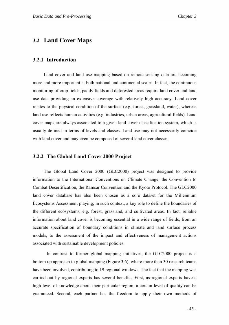
Basic Data and Pre-Processing Chapter 3
- 45 -
3.2 Land Cover Maps
3.2.1 Introduction
Land cover and land use mapping based on remote sensing data are becoming
more and more important at both national and continental scales. In fact, the continuous
monitoring of crop fields, paddy fields and deforested areas require land cover and land
use data providing an extensive coverage with relatively high accuracy. Land cover
relates to the physical condition of the surface (e.g. forest, grassland, water), whereas
land use reflects human activities (e.g. industries, urban areas, agricultural fields). Land
cover maps are always associated to a given land cover classification system, which is
usually defined in terms of levels and classes. Land use may not necessarily coincide
with land cover and may even be composed of several land cover classes.
3.2.2 The Global Land Cover 2000 Project
The Global Land Cover 2000 (GLC2000) project was designed to provide
information to the International Conventions on Climate Change, the Convention to
Combat Desertification, the Ramsar Convention and the Kyoto Protocol. The GLC2000
land cover database has also been chosen as a core dataset for the Millennium
Ecosystems Assessment playing, in such context, a key role to define the boundaries of
the different ecosystems, e.g. forest, grassland, and cultivated areas. In fact, reliable
information about land cover is becoming essential in a wide range of fields, from an
accurate specification of boundary conditions in climate and land surface process
models, to the assessment of the impact and effectiveness of management actions
associated with sustainable development policies.
In contrast to former global mapping initiatives, the GLC2000 project is a
bottom up approach to global mapping (Figure 3.6), where more than 30 research teams
have been involved, contributing to 19 regional windows. The fact that the mapping was
carried out by regional experts has several benefits. First, as regional experts have a
high level of knowledge about their particular region, a certain level of quality can be
guaranteed. Second, each partner has the freedom to apply their own methods of

Chapter 3 Basic Data and Pre-Processing
- 46 -
mapping and define their own regional legend, which allows them to apply the
classification techniques they find as most appropriate for land cover mapping in their
respective region. Third, the regional mapping approach ensures that access could be
gained to reference material. However in order to guarantee the necessary consistency,
the two following conditions had to be fulfilled by the regional experts; i) the data had
to be based on SPOT-4 VEGETATION VEGA2000 dataset, which was made freely
available by CNES, ii) the partners had to use the Land Cover Classification System
which was adopted by FAO (Di Gregorio and Jansen, 2000).
Figure 3.6 The Global Land Cover 2000 Project.
The Central European window was mapped by the Department of
Environmental Sciences and Land Use Planning, at Catholic University of Louvain
(Universite Catholique de Louvain, UCL), Belgium. In the classification process, fifteen
land cover classes have been determined and labelled using a combination of reference
information from the CORINE landcover database (see next sub-section), the
interpretation of high resolution satellite imagery (Landsat TM) and the knowledge of
the local experts. In 2006 the European window classification was updated and the
result is presented in Figure 3.7.
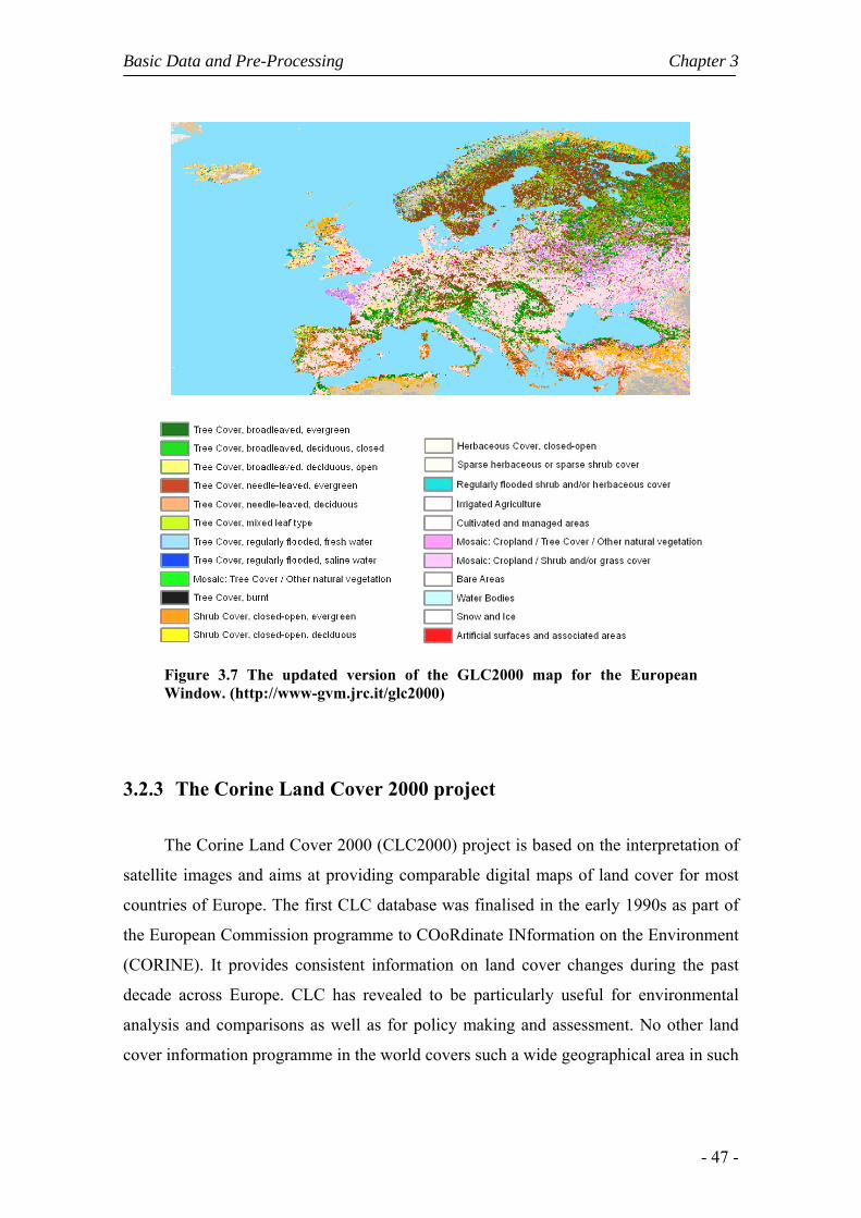
Basic Data and Pre-Processing Chapter 3
- 47 -
Figure 3.7 The updated version of the GLC2000 map for the European Window. (http://www-gvm.jrc.it/glc2000)
3.2.3 The Corine Land Cover 2000 project
The Corine Land Cover 2000 (CLC2000) project is based on the interpretation of
satellite images and aims at providing comparable digital maps of land cover for most
countries of Europe. The first CLC database was finalised in the early 1990s as part of
the European Commission programme to COoRdinate INformation on the Environment
(CORINE). It provides consistent information on land cover changes during the past
decade across Europe. CLC has revealed to be particularly useful for environmental
analysis and comparisons as well as for policy making and assessment. No other land
cover information programme in the world covers such a wide geographical area in such
Chapter 3 Basic Data and Pre-Processing
- 48 -
detail. CLC is recognised by decision-makers as a fundamental thematic reference data
set for spatial and territorial analyses.
At the end of the 1990s several users at national and European levels expressed a
need for its update. The European Environment Agency (EEA) and the Joint Research
Center (JRC) launched the IMAGE2000 and CLC2000 projects, which consisted in the
update of the Corine Land Cover 90 database. Image2000 is a related project to Corine
Land Cover 2000 that provided the necessary Landsat 7 imagery (Figure 3.8) for the
updating of the European Land Use/ Land Cover database.
Figure 3.8 Landsat 7 imagery for the updating CLC, using the IMAGINE2000 software. (http://image2000.jrc.it/)
CLC is therefore a key database for integrated environmental assessment studies,
namely those related with agricultural issues, and provides a pan-European inventory of
biophysical land cover, using a 44 class-nomenclature. In Portugal, the development of
this thematic map was made under the responsibility of Instituto Superior de Estatística
e Gestão da Informação (ISEGI). This Corine Land Cover 2000 for Portugal (Figure
3.9) is originally provided on a 250m by 250m grid, using a Transverse Mercator
projection with the Hayford spheroid. However, the majority of remote sensing imagery
used in this work is defined on geographic coordinates, with 1000m at resolution.
Therefore, in order to enable comparisons of images which had different spatial
resolutions, it was necessary to resample the CLC2000 map to the coarser resolution of
1000m.

Basic Data and Pre-Processing Chapter 3
- 49 -
Figure 3.9 Corine Land Cover 2000 map for Portugal, as developed by ISEGI and the adopted 44 class-nomenclature (http://terrestrial.eionet.europa.eu/ CLC2000).
We started by using the nearest neighbour re-sampling technique because of the
expected good results for less populated classes (Schowengerdt, 1997). Results obtained
for Portugal and for a box centred on the Tagus estuary are shown respectively in
Figures 3.10 and 3.11. When comparing the original maps (left panels of Figures 3.10
and 3.11) with the ones obtained using the nearest neighbour technique (central panels),
it may be observed that some of the classes, e.g. water courses (code 5.1.1) are correctly
resampled, whereas some other classes, e.g. urban areas (codes from 1.1.1 up to 1.4.2)
are less correctly represented.

Chapter 3 Basic Data and Pre-Processing
- 50 -
Figure 3.10 Corine Land Cover 2000 map for Portugal; the original map at 250m resolution (left panel), the degraded map at 1000m resolution using the nearest neighbour technique (central panel), the degraded map at 1000m resolution using the majority rule (right panel).
We have also tested a degradation procedure based on the majority rule that is
commonly applied when degrading thematic maps, namely land cover maps (Turner et
al., 1989; Benson and Mackenzie, 1995; Wu et al., 2002; Saura, 2004). The underlying
assumption is that when applying the majority rule (i.e. the degraded image pixels are
assigned to the most frequent class) similar patterns are produced at coarser resolutions.
Majority rules assign to the degraded image the most frequent class in windows of F×F
pixels, where F, the aggregation factor represents the relation between the length of a
pixel in the degraded and in the original image. When applying this criterion to the
CLC2000 map for Portugal at 250m of resolution in order to obtain a degraded map at
1000m resolution, the procedure involves degradation by a scale factor of 4 in each
direction. The obtained maps, for Continental Portugal and for the box centred in the
Tagus estuary are also shown in Figures 3.10 and 3.11 (right panels). In general, and
independently of the aggregation method used, there is an under representation of the
less frequent classes in the original map. In the case of water courses (code 5.1.1), the
results obtained when using the majority rule were slightly worse than when using the
nearest neighbour technique. However, other equally less frequent classes, e.g. the
urban areas (codes from 1.1.1 up to 1.4.2) present higher spatial consistency when the
majority rule is used.
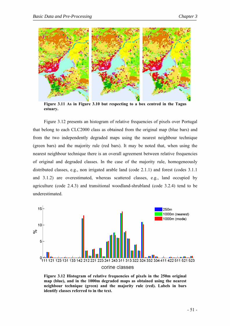
Basic Data and Pre-Processing Chapter 3
- 51 -
Figure 3.11 As in Figure 3.10 but respecting to a box centred in the Tagus estuary.
Figure 3.12 presents an histogram of relative frequencies of pixels over Portugal
that belong to each CLC2000 class as obtained from the original map (blue bars) and
from the two independently degraded maps using the nearest neighbour technique
(green bars) and the majority rule (red bars). It may be noted that, when using the
nearest neighbour technique there is an overall agreement between relative frequencies
of original and degraded classes. In the case of the majority rule, homogeneously
distributed classes, e.g., non irrigated arable land (code 2.1.1) and forest (codes 3.1.1
and 3.1.2) are overestimated, whereas scattered classes, e.g., land occupied by
agriculture (code 2.4.3) and transitional woodland-shrubland (code 3.2.4) tend to be
underestimated.
Figure 3.12 Histogram of relative frequencies of pixels in the 250m original map (blue), and in the 1000m degraded maps as obtained using the nearest neighbour technique (green) and the majority rule (red). Labels in bars identify classes referred to in the text.

Chapter 3 Basic Data and Pre-Processing
- 52 -
The majority rule has however the advantage of assessing the relative presence of
the most frequent class within the 4×4 pixel windows. In fact, when there is the need to
assign pixels to a given class, specific thresholds (e.g. 50%, 75% or 90%) may be
defined in such a way that a pixel is considered as representative of that class when the
relative presence of that class is above the specified threshold. This procedure has the
advantage of providing predefined levels of confidence for each class label, while
maintaining a sufficiently large sample in each class (Lotsch et al., 2003).
Figure 3.13 presents several examples of the obtained spatial distribution of
relative presence for a set of five GLC2000 classes, respectively urban areas (code
1.1.2), non irrigated arable land (code 2.1.1), broad-leaved forest (code 3.1.1), water
courses (code 5.1.1) and estuaries (code 5.2.2). For instance, if there is the need to mask
pixels contaminated by the presence of urban areas or water courses, a low threshold,
e.g. 20%, has to be chosen in order to assure that contamination is adequately
prevented. On the other hand, if the aim is to identify pixels associated to arable land or
to forest a moderate threshold, e.g. 50%, may be appropriate. Finally a high threshold,
e.g. 90% may be chosen if the aim is to study very specific areas, such as estuaries.
1.1.2 2.1.1 3.1.1 5.1.1 5.2.2
Figure 3.13 Spatial distribution of relative presence for a set of five GLC2000 classes for the 1000m degraded maps using the majority rule, respectively urban areas (code 1.1.2), non irrigated arable land (code 2.1.1), broad-leaved forest (code 3.1.1), water courses (code 5.1.1) and estuaries (code 5.2.2).
Basic Data and Pre-Processing Chapter 3
- 53 -
In the present work, the majority rule was used to degrade CLC2000 to 1000m
resolution in order to identify land cover classes that were affected by drought (Chapter
6) and by wildfires (Chapter 7). In Chapter 5 we have defined a threshold of 50% to
produce a 8000 m degraded map of non irrigated arable land (code 2.2.1) in order to
identify areas with wheat crops and monitor the vegetation cycle using GIMMS-NDVI
at 8 km resolution.
3.3 Climate data
3.3.1 Meteorological Data
Meteorological data used in this study are large-scale gridded data as retrieved
from the Climate Research Unit (CRU) datasets, for the period 1982-1999. A complete
description of the methodology used to derive this monthly high-resolution (10’
resolution) climatic database may be found in Mitchell and Jones (2005). This high
resolution dataset replaces the coarser resolution CRU dataset (0.5º x 0.5º) widely used
in many climatic variability studies over Europe (e.g. Trigo et al., 2004; Paredes et al.,
2006). This dataset was built based on an optimum interpolation method that takes into
account latitude, longitude, and elevation using thin-plate splines (New et al., 1999;
2000). The accuracy of the obtained interpolations is assessed using cross validation as
well as through objective comparisons with other climatologies. The higher resolution
database was checked for inhomogeneities in the station records, by means of an
automated procedure that refines previous methods using incomplete and partially
overlapping records and through the detection of inhomogeneities with opposite signs in
different seasons (Mitchell and Jones, 2005).
Monthly values of cloud cover, temperature and precipitation, were extracted
from the CRU database for the window 35ºN-45ºN, 10ºW-0ºE. Under the scope of the
Portuguese funded (FCT/ESA) project CARBERIAN (Terrestrial Vegetation Carbon
Trends in the Iberian Peninsula), the CRU TS 1.2 10’ climate datasets were interpolated
to the GIMMS NDVI coordinates grid with a recently developed non-linear method
(Zhao et al., 2005). The cloud cover time series were then converted to net solar
radiation fields using the Soil and Water Assessment Tool, a method developed by

Chapter 3 Basic Data and Pre-Processing
- 54 -
Neitsch et al. (2002). This procedure yielded monthly climate fields geographically
compatible with GIMMS NDVI.
The Global Precipitation Climatology Project (GPCP) is an element of the Global
Energy and Water Cycle Experiment (GEWEX) of the World Climate Research
program (WCRP). It was established by the WCRP in 1986 with the major aim of
providing monthly mean precipitation data on a 2.5°×2.5° latitude/longitude grid.
Monthly mean precipitation estimates are being produced continuously since 1979. In
this dataset infrared and microwave satellite estimates of precipitation were merged
with rain gauge data from more than 6,000 stations. Infrared precipitation estimates are
obtained from GOES (United States), GMS (Japan) and Meteosat (European
Community) geostationary satellites as well as from the National Oceanic and
Atmospheric Administration (NOAA) operational polar orbiting satellites. Microwave
estimates are obtained from the U.S. Defense Meteorological Satellite Program (DMSP)
satellites using the Special Sensor Microwave Imager (SSM/I). These data sets will be
used to validate general circulation and climate models, to study the global hydrological
cycle and to diagnose the variability of the global climate system.
In recent years the data sets have been updated and enlarged, to that besides the
monthly mean product available, the GPCP has now a 2.5°×2.5° degree pentad data set
since 1979, a 1°×1° daily data set since 1997 and (on request) the 0.5º×0.5º grid
monthly data. Here we have used monthly precipitation data from the GPCC (Rudolf
and Schneider, 2005) with the highest resolution (0.5º latitude by 0.5º longitude grid),
covering the period 1982-2002 for the European window.
3.3.2 North Atlantic Oscillation
The North Atlantic Oscillation (NAO) has been recognized for more than 70
years as one of the major patterns of atmospheric variability in the Northern
Hemisphere (Walker, 1924). The NAO refers to a meridional oscillation of the
atmospheric mass with centers of action located near Iceland and over the subtropical
Atlantic from the Azores across the Iberian Peninsula. When NAO is in its positive
phase, low pressure anomalies over the Icelandic region and throughout the Arctic
combine with high-pressure anomalies across the subtropical Atlantic to produce
Basic Data and Pre-Processing Chapter 3
- 55 -
stronger than average westerlies across the midlatitudes. Therefore, this phase of the
oscillation is associated with cold conditions over the northwest Atlantic and warm
weather over Europe, together with wet conditions from Iceland through Scandinavia
and dry conditions over southern Europe.
However, only in recent years has this important atmospheric circulation mode
become the subject of a wider interest (e.g. van Loon and Rogers, 1978; Rogers, 1984;
Barnston and Livezey, 1987). More recently, the study by Hurrell (1995) had significant
impact on the climatological community and has been followed by an increasing
number of studies. It is within this context, that several studies have established links
between the NAO index and winter season precipitation in Western Europe and, in
particular, over the Mediterranean basin (Hurrell 1995; Qian et al., 2000; Trigo et al.,
2004). This control exerted by NAO on the precipitation field over Europe is likely
related to corresponding changes in the associated activity of North Atlantic storm
tracks (Serreze et al., 1997; Osborn et al., 1999). In fact, this strong NAO-precipitation
link has been used to develop rainfall forecast models that predict precipitation in Iberia
several months in advance (e.g. Gámiz-Fortis et al, 2002; Rodriguez-Fonseca and
Castro, 2002). The output of these models may provide useful seasonal forecasting tools
for water resource managers and risk assessment teams (Trigo et al., 2004).
The NAO index used in this study is based on the one developed by the Climatic
Research Unit (University of East Anglia, UK) which was originally defined, on a
monthly basis, as the difference between the normalized surface pressure at Gibraltar, in
the southern tip of the Iberian Peninsula and Stykkisholmur, in Iceland (Jones et al.,
1997). For each year covering the 21-year long period from 1982 to 2002, we have
derived a late winter NAO index, defined as the average of the monthly values of
January, February and March of the corresponding year. In this work we will use the
term NAO to refer to the three-monthly averaged as well as to any averaged quantity
over January, February and March (e.g, PNAO for averaged precipitation). It may be
finally noted that the original time series of winter monthly values of the NAO index
presents a positive trend over the last 30 years and therefore its distribution is
dominated by positive values, leading to late winter averages above zero (Jones et al.,
1997). As a representative example, Figure 3.14 shows the patterns of simple
correlation computed over the period 1982-2002 the three monthly averages of winter
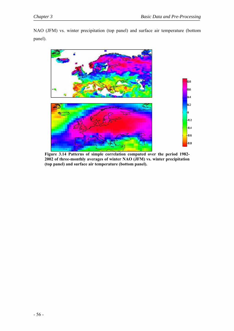
Chapter 3 Basic Data and Pre-Processing
- 56 -
NAO (JFM) vs. winter precipitation (top panel) and surface air temperature (bottom
panel).
Figure 3.14 Patterns of simple correlation computed over the period 1982-2002 of three-monthly averages of winter NAO (JFM) vs. winter precipitation (top panel) and surface air temperature (bottom panel).

4. CLIMATE IMPACT ON VEGETATION DYNAMICS
4.1 Introduction
Over the last two decades, the continuous monitoring of vegetation from space
has prompted new studies aiming to relate the observed major global changes in
vegetation (e.g. trends, variability and extremes) with changes of surface climatic
variables, such as temperature and precipitation (Myneni et al., 1997, Hansen et al.,
1999, Zhou et al., 2001). In particular, several groups have shown that the recorded rise
of temperature in the northern latitudes by 0.8ºC in the last 25 years has been
accompanied by a significant reduction in annual snow cover as induced by an early
melting of snow in spring (Groisman et al., 1994, Vinnikov et al., 1999). A longer
active growing season has also been observed as a result of an early spring and delayed
autumn (Bogaert et al., 2002, Shabanov et al., 2002). This change in the annual cycle is
associated with an increase in photosynthetic activity of vegetation (Zhou et al., 2001),
as detected from observed changes in the Normalised Difference Vegetation Index
(NDVI).
Although no evidence has been given that such changes in NDVI are related to the
positive trend in atmospheric concentration of CO2 (Kaufmann et al., 2002), the global
carbon cycle has been certainly affected (Keeling et al., 1996) and there is a strong need
for long-term and large-scale studies aiming to assess the impact of atmospheric
circulation variability on surface climate and related vegetation activity. In this respect
special attention has been devoted to investigating relationships between vegetation
dynamics and the North Atlantic Oscillation (NAO), which (as shown in Chapter 3) is
the major pattern of atmospheric variability in the Northern Hemisphere (Hurrell, 1995).
A number of studies have naturally addressed the question of the relationship between
NDVI and meteorological fields, namely temperature and precipitation. Vicente-Serrano
and Heredia-Laclaustra (2004) have adopted the climatological viewpoint and focused
their attention on the Iberian Peninsula where the influence of winter NAO on the

Chapter 4 Climate Impact on Vegetation Dynamics
- 58 -
precipitation regime is especially prominent in the south-west region (Rodriguez-Puebla
et al., 1998). They have shown the existence of a positive trend in annual vegetation
productivity where the NAO influence is weaker, in strong contrast to the stable or
negative trends that were detected in the areas located in the south of Iberia, where
precipitation is mostly determined by NAO. However the authors pointed out the need
for further studies, at finer temporal scales, namely at the monthly and seasonal ones.
Stöckli and Vidale (2004) have found that spring plant phenology over Europe is
well correlated with the winter NAO index. Their study has focused on several
geographical sub-domains of Europe that neither reflect any bio-geographical
stratification nor any particular sensitivity to the NAO index. The Mediterranean and, in
particular, the Iberian Peninsula was not included in the study because their analysis
procedure required a large seasonal amplitude in the phenology. The aim of the present
chapter is to fill the gap between the assessment made by land cover experts and by
researchers that have looked at the problem from a climatological viewpoint. We will
search for relationships between NAO and vegetation activity at the month and seasonal
levels over Europe and look for regions where such activity presents a clear dependence
on NAO both in spring and summer. We will then investigate how such dependence
may be explained in terms of the impact of NAO on relevant surface climate variables,
namely temperature and precipitation. We will pay special attention to the Iberian
Peninsula and Northeastern Europe because of the distinctive vegetation response to
precipitation and temperature. Finally, we will identify which of the variables have a
determinant role on vegetation activity of different regions and make an assessment on
the role played by the variables in the annual cycle of vegetation activity.
Accordingly, the main goals of this chapter are the following:
• To study the relation between vegetation phenology and NAO over Europe.
• To characterise the vegetation response to precipitation and temperature in two
contrasting areas of Europe, respectively Northeastern Europe and the Iberian
Peninsula.
• To assess the impact of NAO on the vegetative cycle in the two areas, and relate it
to the different land cover types and their response to surface climate variability.

Climate Impact on Vegetation Dynamics Chapter 4
- 59 -
Relationships between NAO and diverse aspects of European vegetation
dynamics have been addressed by various authors. D’Odorico et al. (2002) showed that
spring phenology in the British Isles is influenced by NAO. Dates of leaf unfolding for
a mean of nine plant species vary over a 40-day range, from approximately the spring
equinox to the end of April. The Julian date of leaf unfolding is inversely correlated
with the NAO phase, i.e. leaf unfolding occurs earlier under positive, and later under
negative phases of NAO. Similar patterns are reported for Poland, Norway and Sardinia.
D’Odorico et al. (2002) also found a strong NAO influence on the timing of the pollen
season in Europe.
Cook et al. (2004) modelled the NAO-dependence of phenological variability in
Europe, mediated by the NAO influence on synoptic scale winter temperature
variability, and successfully reproduced observed patterns of growing degree-days over
Europe. A projection of NAO trends 50 years into the future, based on climate change
scenarios, indicated a sustained advance of the growing season start.
Stöckli and Vidale (2004) used AVHRR Pathfinder NDVI data, and found that
spring phenology correlates well with anomalies in winter temperature and winter NAO
index. They established the existence of trends towards an earlier onset and longer
duration of the spring vegetation growing period, especially significant over Central
Europe.
Vicente-Serrano and Heredia-Laclaustra (2004) analysed the relationship between
the NAO index and vegetation productivity (represented by the annual integral of
monthly AVHRR Pathfinder NDVI values) trends, for the Iberian Peninsula. Areas of
stable or decreasing vegetation productivity were located in southern Iberia, where the
NAO influence is stronger. Significant positive productivity trends occur in the north of
the Peninsula, where the NAO influence on vegetation dynamics is weaker.
We will rely on AVHRR NDVI data from the Global Inventory Modelling and
Mapping Studies – GIMMS group (see Chapter 3), which incorporate more thorough
and accurate corrections of orbital drift, radiometric degradation, and volcanic aerosol
effects than those previously applied to the Pathfinder AVHRR Land (PAL) product,
used in earlier works.
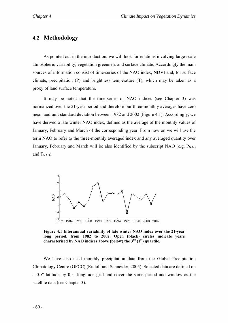
Chapter 4 Climate Impact on Vegetation Dynamics
- 60 -
4.2 Methodology
As pointed out in the introduction, we will look for relations involving large-scale
atmospheric variability, vegetation greenness and surface climate. Accordingly the main
sources of information consist of time-series of the NAO index, NDVI and, for surface
climate, precipitation (P) and brightness temperature (T), which may be taken as a
proxy of land surface temperature.
It may be noted that the time-series of NAO indices (see Chapter 3) was
normalized over the 21-year period and therefore our three-monthly averages have zero
mean and unit standard deviation between 1982 and 2002 (Figure 4.1). Accordingly, we
have derived a late winter NAO index, defined as the average of the monthly values of
January, February and March of the corresponding year. From now on we will use the
term NAO to refer to the three-monthly averaged index and any averaged quantity over
January, February and March will be also identified by the subscript NAO (e.g. PNAO
and TNAO).
Figure 4.1 Interannual variability of late winter NAO index over the 21-year long period, from 1982 to 2002. Open (black) circles indicate years characterised by NAO indices above (below) the 3rd (1st) quartile.
We have also used monthly precipitation data from the Global Precipitation
Climatology Centre (GPCC) (Rudolf and Schneider, 2005). Selected data are defined on
a 0.5º latitude by 0.5º longitude grid and cover the same period and window as the
satellite data (see Chapter 3).
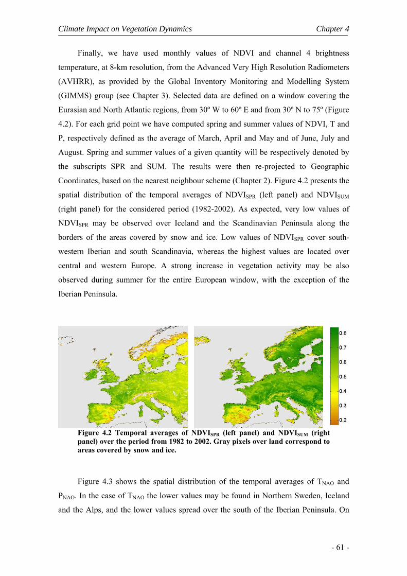
Climate Impact on Vegetation Dynamics Chapter 4
- 61 -
Finally, we have used monthly values of NDVI and channel 4 brightness
temperature, at 8-km resolution, from the Advanced Very High Resolution Radiometers
(AVHRR), as provided by the Global Inventory Monitoring and Modelling System
(GIMMS) group (see Chapter 3). Selected data are defined on a window covering the
Eurasian and North Atlantic regions, from 30º W to 60º E and from 30º N to 75º (Figure
4.2). For each grid point we have computed spring and summer values of NDVI, T and
P, respectively defined as the average of March, April and May and of June, July and
August. Spring and summer values of a given quantity will be respectively denoted by
the subscripts SPR and SUM. The results were then re-projected to Geographic
Coordinates, based on the nearest neighbour scheme (Chapter 2). Figure 4.2 presents the
spatial distribution of the temporal averages of NDVISPR (left panel) and NDVISUM
(right panel) for the considered period (1982-2002). As expected, very low values of
NDVISPR may be observed over Iceland and the Scandinavian Peninsula along the
borders of the areas covered by snow and ice. Low values of NDVISPR cover south-
western Iberian and south Scandinavia, whereas the highest values are located over
central and western Europe. A strong increase in vegetation activity may be also
observed during summer for the entire European window, with the exception of the
Iberian Peninsula.
Figure 4.2 Temporal averages of NDVISPR (left panel) and NDVISUM (right panel) over the period from 1982 to 2002. Gray pixels over land correspond to areas covered by snow and ice.
Figure 4.3 shows the spatial distribution of the temporal averages of TNAO and
PNAO. In the case of TNAO the lower values may be found in Northern Sweden, Iceland
and the Alps, and the lower values spread over the south of the Iberian Peninsula. On
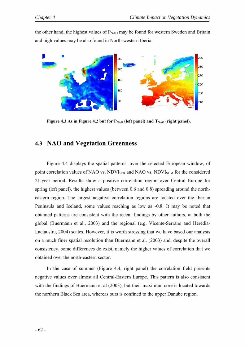
Chapter 4 Climate Impact on Vegetation Dynamics
- 62 -
the other hand, the highest values of PNAO may be found for western Sweden and Britain
and high values may be also found in North-western Iberia.
Figure 4.3 As in Figure 4.2 but for PNAO (left panel) and TNAO (right panel).
4.3 NAO and Vegetation Greenness
Figure 4.4 displays the spatial patterns, over the selected European window, of
point correlation values of NAO vs. NDVISPR and NAO vs. NDVISUM for the considered
21-year period. Results show a positive correlation region over Central Europe for
spring (left panel), the highest values (between 0.6 and 0.8) spreading around the north-
eastern region. The largest negative correlation regions are located over the Iberian
Peninsula and Iceland, some values reaching as low as -0.8. It may be noted that
obtained patterns are consistent with the recent findings by other authors, at both the
global (Buermann et al., 2003) and the regional (e.g. Vicente-Serrano and Heredia-
Laclaustra, 2004) scales. However, it is worth stressing that we have based our analysis
on a much finer spatial resolution than Buermann et al. (2003) and, despite the overall
consistency, some differences do exist, namely the higher values of correlation that we
obtained over the north-eastern sector.
In the case of summer (Figure 4.4, right panel) the correlation field presents
negative values over almost all Central-Eastern Europe. This pattern is also consistent
with the findings of Buermann et al (2003), but their maximum core is located towards
the northern Black Sea area, whereas ours is confined to the upper Danube region.

Climate Impact on Vegetation Dynamics Chapter 4
- 63 -
Figure 4.4 Point correlation fields of NAO vs. NDVISPR (left panel) and NAO vs. NDVISUM (right panel) over the period from 1982 to 2002. Black frames identify the Baltic region and the Iberian Peninsula. The colorbar identifies values of correlation and the two arrows indicate the ranges that are significant at 5% level.
The contrasting behaviour of north-eastern and south-western regions of Europe is
worth being further investigated. For this purpose we have selected two regions, namely
Northeastern Europe (hereafter NE) and the Iberian Peninsula (hereafter IB). These two
regions are identified by black frames in Figure 4.4 and it may be noted that selection
was made in such a way to obtain an amount of land pixels of the same order in the two
regions, respectively 9639 over NE and 9080 over IB. Both NE and IB show fairly
coherent values of correlation of NAO vs. NDVI for both spring and summer. It is also
apparent that over IB, NAO is anti-correlated with vegetation greenness both in spring
and summer, whereas over NE the correlation is positive in spring and predominantly
negative in summer. During spring, the distribution of correlation values over NE
presents a median value about 0.5, whereas the distribution over IB has a median of -0.2
and spans a wide range of negative values, reaching as low as -0.7 (Figure 4.5). During
summer, both areas exhibit distributions with similar medians about -0.2, but the lower
dispersion is now observed over IB.
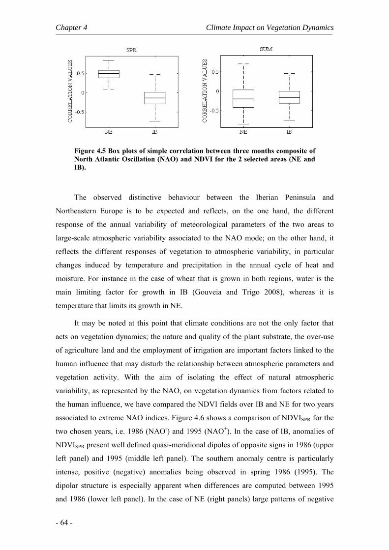
Chapter 4 Climate Impact on Vegetation Dynamics
- 64 -
Figure 4.5 Box plots of simple correlation between three months composite of North Atlantic Oscillation (NAO) and NDVI for the 2 selected areas (NE and IB).
The observed distinctive behaviour between the Iberian Peninsula and
Northeastern Europe is to be expected and reflects, on the one hand, the different
response of the annual variability of meteorological parameters of the two areas to
large-scale atmospheric variability associated to the NAO mode; on the other hand, it
reflects the different responses of vegetation to atmospheric variability, in particular
changes induced by temperature and precipitation in the annual cycle of heat and
moisture. For instance in the case of wheat that is grown in both regions, water is the
main limiting factor for growth in IB (Gouveia and Trigo 2008), whereas it is
temperature that limits its growth in NE.
It may be noted at this point that climate conditions are not the only factor that
acts on vegetation dynamics; the nature and quality of the plant substrate, the over-use
of agriculture land and the employment of irrigation are important factors linked to the
human influence that may disturb the relationship between atmospheric parameters and
vegetation activity. With the aim of isolating the effect of natural atmospheric
variability, as represented by the NAO, on vegetation dynamics from factors related to
the human influence, we have compared the NDVI fields over IB and NE for two years
associated to extreme NAO indices. Figure 4.6 shows a comparison of NDVISPR for the
two chosen years, i.e. 1986 (NAO-) and 1995 (NAO+). In the case of IB, anomalies of
NDVISPR present well defined quasi-meridional dipoles of opposite signs in 1986 (upper
left panel) and 1995 (middle left panel). The southern anomaly centre is particularly
intense, positive (negative) anomalies being observed in spring 1986 (1995). The
dipolar structure is especially apparent when differences are computed between 1995
and 1986 (lower left panel). In the case of NE (right panels) large patterns of negative

Climate Impact on Vegetation Dynamics Chapter 4
- 65 -
(positive) anomalies of NDVISPR may be observed in 1986 (1995). Observed anomalies
are particularly intense in 1986 (NAO-) and this feature is well apparent when analysing
differences between 1995 and 1986 (lower right panel).
Figure 4.6 Seasonal anomalies of NDVISPR for 1986 (NAO+), 1995 (NAO-) and for differences between 1995 and 1986 (upper, middle and lower panels, respectively) over IB and NE (left and right panels respectively).
4.4 NAO and Climatic Activity
Taking into account the results of the previous section, we will now pay attention
to the influence of the NAO mode over two atmospheric parameters relevant to
vegetation activity, namely surface temperature and precipitation. The analysis will
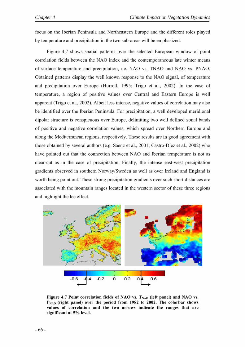
Chapter 4 Climate Impact on Vegetation Dynamics
- 66 -
focus on the Iberian Peninsula and Northeastern Europe and the different roles played
by temperature and precipitation in the two sub-areas will be emphasized.
Figure 4.7 shows spatial patterns over the selected European window of point
correlation fields between the NAO index and the contemporaneous late winter means
of surface temperature and precipitation, i.e. NAO vs. TNAO and NAO vs. PNAO.
Obtained patterns display the well known response to the NAO signal, of temperature
and precipitation over Europe (Hurrell, 1995; Trigo et al., 2002). In the case of
temperature, a region of positive values over Central and Eastern Europe is well
apparent (Trigo et al., 2002). Albeit less intense, negative values of correlation may also
be identified over the Iberian Peninsula. For precipitation, a well developed meridional
dipolar structure is conspicuous over Europe, delimiting two well defined zonal bands
of positive and negative correlation values, which spread over Northern Europe and
along the Mediterranean regions, respectively. These results are in good agreement with
those obtained by several authors (e.g. Sáenz et al., 2001; Castro-Díez et al., 2002) who
have pointed out that the connection between NAO and Iberian temperature is not as
clear-cut as in the case of precipitation. Finally, the intense east-west precipitation
gradients observed in southern Norway/Sweden as well as over Ireland and England is
worth being point out. These strong precipitation gradients over such short distances are
associated with the mountain ranges located in the western sector of these three regions
and highlight the lee effect.
Figure 4.7 Point correlation fields of NAO vs. TNAO (left panel) and NAO vs. PNAO (right panel) over the period from 1982 to 2002. The colorbar shows values of correlation and the two arrows indicate the ranges that are significant at 5% level.

Climate Impact on Vegetation Dynamics Chapter 4
- 67 -
Although it is known that the impact of NAO on temperature and precipitation
described above is especially prominent in winter (e.g. Vicente-Serrano and Heredia-
Laclaustra, 2004, Trigo et al., 2004), such behaviour contrasts with that obtained for
vegetation activity (Figure 4.4), where the impact of NAO is clearly apparent both in
spring and summer (i.e. NAO vs. NDVISPR and NAO vs. NDVISUM). This gives a strong
indication that special attention must be devoted to the relationship between late winter
temperature and late winter precipitation, with vegetation greenness in the following
spring and summer seasons.
Since we are particularly interested in pixels characterised by the strong influence
of NAO on vegetation activity, we will restrict our analysis to IB and NE (as identified
in Figure 4.4), and will focus on those pixels that exhibit the highest (lowest) values of
positive (negative) correlations of NDVISPR and NDVISUM with NAO. Henceforth, they
will be called NAO High Correlation Pixels (NHCP).
As pointed out in the previous section, vegetation greenness over the IB is
negatively correlated with NAO, both in spring and summer. Accordingly, we selected,
for each one of the two seasons, the 500 highest NHCP. In the case of NE, NHCP were
predominantly correlated with NDVI in spring and anti-correlated in summer. Therefore
we selected the 500 pixels with the highest (lowest) values of positive (negative)
correlation in spring (summer). Figures 4.8 and 4.9 show the geographical distribution
of the NHCP for spring and summer, respectively over IB and NE. Information about
the land cover type associated to each pixel is also provided, as obtained from the
Global Land Cover 2000 (GLC2000) database (Chapter 3). Table 4.1 shows descriptive
statistics of the NHCP associated with the two most common types of vegetation
namely in what respects to the distribution of NDVI anomalies for two classes of years,
characterised by extreme NAO indices, i.e. the NAO+ and NAO-, as described in section
3. NDVI anomalies in a given pixel are defined as differences from the respective 21-
year mean (1982-2002) and the two considered classes of years. For each area and
season the statistical distributions of NDVI anomaly values for the two classes of years
(NAO+ and NAO-) and the two types of vegetation cover are characterised by means of
the respective median (Q2), first and third quartiles (Q1 and Q3), and percentiles 1 and
99 (P1 and P99).

Chapter 4 Climate Impact on Vegetation Dynamics
- 68 -
As expected, there are marked differences in the obtained distributions of NDVI
anomalies for NAO+ and NAO- classes for a given type of vegetation, in a given season,
over a given region. For instance, it is worth noting that there is no class overlap when
restricting to median values between P1 and P99. This feature was taken into account in
Figures 4.8 and 4.9, where a given year is characterised by its median value.
Figure 4.8 Geographical distribution of sets of selected pixels over the IB (upper panels), based on the strong values of correlation of NDVISPR (upper left panel) and NDVISUM (upper right panel) with NAO. Red, green and blue pixels are respectively associated to forest and shrub, cultivated areas and other types of vegetation cover. Land cover type (low panel) as obtained from GLC2000).
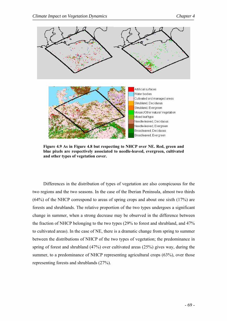
Climate Impact on Vegetation Dynamics Chapter 4
- 69 -
Figure 4.9 As in Figure 4.8 but respecting to NHCP over NE. Red, green and blue pixels are respectively associated to needle-leaved, evergreen, cultivated and other types of vegetation cover.
Differences in the distribution of types of vegetation are also conspicuous for the
two regions and the two seasons. In the case of the Iberian Peninsula, almost two thirds
(64%) of the NHCP correspond to areas of spring crops and about one sixth (17%) are
forests and shrublands. The relative proportion of the two types undergoes a significant
change in summer, when a strong decrease may be observed in the difference between
the fraction of NHCP belonging to the two types (29% to forest and shrubland, and 47%
to cultivated areas). In the case of NE, there is a dramatic change from spring to summer
between the distributions of NHCP of the two types of vegetation; the predominance in
spring of forest and shrubland (47%) over cultivated areas (25%) gives way, during the
summer, to a predominance of NHCP representing agricultural crops (63%), over those
representing forests and shrublands (27%).

Chapter 4 Climate Impact on Vegetation Dynamics
- 70 -
Table 4.1 Descriptive statistics of the distributions of NDVI anomalies for NAO High Correlation Pixels (NHCP) associated to the two most important vegetation types as found in the cases of spring and summer over IB and NE. P1, Q1, Q2, Q3 and P99 respectively denote percentile one, the first quartile, the median, the third quartile and percentile 99. Percent figures in parenthesis below the types of vegetation indicate the fraction of pixels of the considered NHCP associated to that type.
IB Spring
Forest & shrubland (17%) *
Cultivated (64%)
P1 Q1 Q2 Q3 P99 P1 Q1 Q2 Q3 P99 NAO+ -0,049 -0,030 -0,021 -0,013 0,002 -0,080 -0,041 -0,031 -0,022 -0,004NAO- 0,004 0,015 0,024 0,033 0,066 0,003 0,019 0,027 0,038 0,071
Summer Forest & shrubland
(29%) ** Cultivated
(47%) P1 Q1 Q2 Q3 P99 P1 Q1 Q2 Q3 P99
NAO+ -0,053 -0,031 -0,023 -0,017 0,005 -0,066 -0,036 -0,026 -0,014 0,000 NAO- -0,001 0,011 0,016 0,022 0,039 0,003 0,012 0,018 0,025 0,054
NE
Spring Needle-leaved Evergreen
(47%)# Cultivated
(25%) P1 Q1 Q2 Q3 P99 P1 Q1 Q2 Q3 P99 NAO+ 0,011 0,027 0,033 0,041 0,071 0,009 0,026 0,033 0,044 0,060NAO- -0,084 -0,054 -0,043 -0,035 -0,014 -0,072 -0,055 -0,045 -0,037 -0,010
Summer Needle-leaved Evergreen
(27%)## Cultivated
(63%) P1 Q1 Q2 Q3 P99 P1 Q1 Q2 Q3 P99 NAO+ -0,059 -0,037 -0,028 -0,021 -0,008 -0,068 -0,039 -0,030 -0,022 -0,005NAO- 0,006 0,020 0,025 0,032 0,056 0,009 0,022 0,027 0,034 0,052
* Includes 14% of Needle-leaved Evergreen, 26% of Broadleaved deciduous and 60% of Shrubland. ** Includes 31% of Needle-leaved Evergreen, 25% of Broadleaved deciduous and 44% of Shrubland # Includes 12% of Needle-leaved Evergreen and 88% de Broadleaved deciduous ## Includes 35% of Needle-leaved Evergreen and 65% de Broadleaved deciduous
The above results may be viewed in terms of the distinct responses of the various
vegetation types to moisture and heat conditions prevailing during the previous winter.
These conditions, in turn, are determined by the nature of the relationships between the
surface annual variability of atmospheric parameters, PNAO and TNAO, and the different
phases (NAO+ and NAO-) of the NAO atmospheric mode. Figures 4.10 and 4.11 show
scatterplots, for IB and NE, respectively, of spring and summer anomalies of vegetation
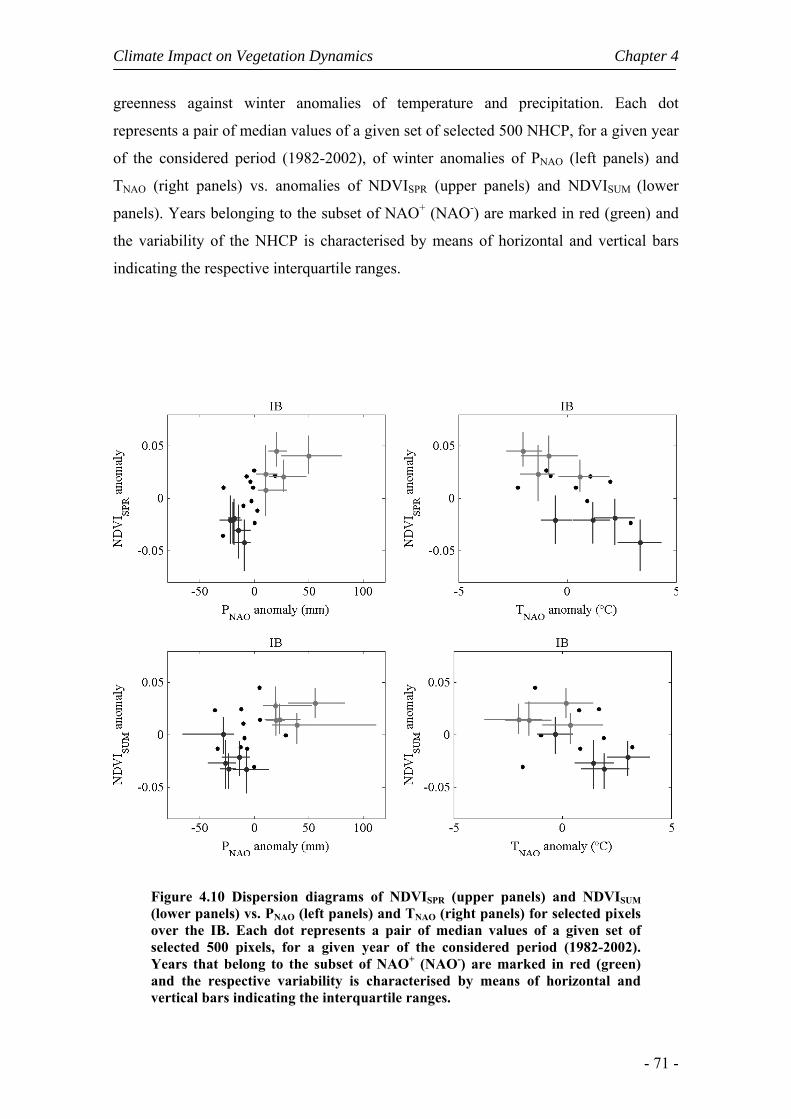
Climate Impact on Vegetation Dynamics Chapter 4
- 71 -
greenness against winter anomalies of temperature and precipitation. Each dot
represents a pair of median values of a given set of selected 500 NHCP, for a given year
of the considered period (1982-2002), of winter anomalies of PNAO (left panels) and
TNAO (right panels) vs. anomalies of NDVISPR (upper panels) and NDVISUM (lower
panels). Years belonging to the subset of NAO+ (NAO-) are marked in red (green) and
the variability of the NHCP is characterised by means of horizontal and vertical bars
indicating the respective interquartile ranges.
Figure 4.10 Dispersion diagrams of NDVISPR (upper panels) and NDVISUM (lower panels) vs. PNAO (left panels) and TNAO (right panels) for selected pixels over the IB. Each dot represents a pair of median values of a given set of selected 500 pixels, for a given year of the considered period (1982-2002). Years that belong to the subset of NAO+ (NAO-) are marked in red (green) and the respective variability is characterised by means of horizontal and vertical bars indicating the interquartile ranges.

Chapter 4 Climate Impact on Vegetation Dynamics
- 72 -
Figure 4.11 As in Figure 4.10, but respecting to NE.
As shown in Figure 4.10, IB region presents a similar spring and summer
vegetation response to precipitation, i.e. an increase (decrease) of vegetation greenness
for NAO- (NAO+) years. In both seasons there is less variability of precipitation in the
set of NAO+ NHCP, in comparison with NAO-, especially in spring. A slight
dependence of vegetation greenness on temperature is also apparent in the case of
spring, with NVDISPR median values showing a tendency to decrease from NAO- to
NAO+. It may be noted that the obtained stronger dependence of vegetation on
precipitation than on temperature is consistent with the already pointed out fact that
over the Iberian Peninsula the influence of NAO is particularly strong on the
precipitation regime whereas the relationship between NAO and temperature is less
clear. In the case of NE (Figure 4.11) there is a marked dependence of vegetation
greenness on winter temperature, but the nature of such dependence is reversed from
spring to summer. In the first case, NDVISPR shows a strong increase from NAO- to
NAO+, whereas a sharp decrease is observed for summer. The lower variability of
temperature in the set NHCP for NAO+ is again evident, when compared with the

Climate Impact on Vegetation Dynamics Chapter 4
- 73 -
corresponding set for NAO-. Concerning winter precipitation, no effects are apparent on
vegetation greenness for both spring and summer. Finally, the differences in magnitude
of the impacts of NAO on precipitation and temperature in IB and NE is worth being
emphasised; the impact on precipitation (temperature) is three times larger over IB (NE)
than the corresponding impact over NE (IB), a feature that is in good agreement with
the found dependences of NDVI on precipitation (temperature) over IB (NE). This is to
be expected, since vegetation growth is much more water-limited in IB than in NE.
4.5 The role NAO on the vegetative cycle
The striking differences that were obtained in the response of vegetation to
moisture and heat conditions and to anomalies in PNAO and TNAO associated to the NAO
atmospheric mode, warrant further analysis of the NDVI annual cycle for the NHCP
over IB and NE. Figure 4.12 presents the annual cycles of NDVI monthly values for the
NHCP, for spring (upper panels) and summer (lower panels), over IB (left panels) and
NE (right panels). The annual cycles of mean NDVI for the entire period (1982-2002)
are represented by thick solid black lines, whereas the annual cycles of averages for the
NAO- (NAO+) subsets are identified by the thin solid (dashed) curves.
In the case of IB the most interesting feature for both spring and summer (Figure
4.12, left panels) is that the highest impact of NAO is observed to occur during the
periods of the year characterised by more intense vegetation activity (Ji and Peters,
2003), i.e. around April (June) in the case of the NHCP for spring (summer). During
spring, two thirds of the NHCP (Table 4.1) correspond to cultivated areas that mainly
consist of crops adapted to the relatively dry Iberian conditions. Due to the generally
observed high temperatures, vegetation has a short growth cycle that starts as soon as
water is available, a situation that is especially favoured by NAO-. This is especially
apparent in Figure 4.13 (left panel) where the annual cycles of NDVI are compared for
the years of 1986 (NAO-) and 1995 (NAO+) that were chosen because of being
associated to extreme NAO indices. In the case of summer the vegetation that is most
affected by NAO initiates its growing period late in the year and therefore the response
to precipitation tends to extend late in the year.

Chapter 4 Climate Impact on Vegetation Dynamics
- 74 -
Figure 4.12 Annual cycles of monthly values of NDVI for NAO High Correlation Pixels (NHCP), for spring (upper panel) and summer (lower panel), over IB (left panel) and NE (right panel). The annual cycles of average NDVI values for the entire period (1982-2002) are represented by thick solid lines, whereas the annual cycles of averages for the NAO- (NAO+) subsets are identified by the thin solid (dashed) curves. Vertical dashed curves delimit the season of the year.
Figure 4.13As in Figure 4.12, but restricting to the annual cycles of NDVI for the individual years of 1986 (NAO−) and 1995 (NAO+), respectively represented by the dashed and the solid lines.

Climate Impact on Vegetation Dynamics Chapter 4
- 75 -
In the case of NE (Figure 4.13, right panels) the annual cycles present
characteristics that are very different from those observed over IB. The impact of NAO
is especially conspicuous during the first months of the year, suggesting that green
vegetation growth tends to occur early and intensively, due to the combined effect of
warm conditions, especially of the former, since water availability is seldom a problem
in NE. This contrast in the response of vegetation during the early months is also well
apparent in Figure 4.13 (right panel) where the years of 1986 (NAO-) and 1995 (NAO+)
are compared. The distinct behaviour of vegetation in spring (Figure 4.12, upper panel)
and summer (lower panel) is also worth pointing out. In the case of the spring, the NAO
impact is almost negligible, whereas in the case of the summer the growth of vegetation
is enhanced under NAO- conditions. This is to be expected, since snow melt is expected
to occur later in the year, due to the lower winter temperature. Accordingly, vegetation
growth will be reduced in spring, getting delayed until summer, when solar radiation
availability increases (Blenckner and Hillebrand, 2002; Menzel 2003; Wang and You,
2004).
4.6 Conclusions
We analysed the relationship between the NAO atmospheric mode and vegetation
activity (NDVI) over the two contrasting regions of Iberia and Northeastern Europe. As
expected the behaviour of vegetation reflects the different response of surface climate to
large-scale atmospheric variability associated to the NAO mode. A systematic analysis
was performed over two contrasting regions of Europe, namely IB and NE. Over IB
there is strong evidence that positive (negative) values of winter NAO induce low (high)
vegetation activity in the following spring and summer seasons. This feature is mainly
associated with the impact of NAO on winter precipitation, together with the strong
dependence of spring and summer NDVI on contemporary water availability. NE shows
a different behaviour, with positive (negative) values of winter NAO inducing high
(low) values of NDVI in spring, but low (high) values of NDVI in summer. This
behaviour mainly results from the strong impact of NAO on winter temperature
associated with the critical dependence of vegetation growth on the combined effect of
warm conditions and water availability during the winter season. (D’Odorico et al.,
2002).
Chapter 4 Climate Impact on Vegetation Dynamics
- 76 -
In both spring and summer NHCP over the Iberian Peninsula there is less
precipitation variability under NAO+ than under NAO-, especially in the spring. This
feature may be associated with the strong impact of climate variability in semi-arid
areas, namely regarding effects of drought conditions on vegetation activity (Vicente-
Serrano and Heredia-Laclaustra, 2004), in particular during the intense spring
vegetation growth period. A weak dependence of vegetation greenness on temperature
is also visible in spring, with median values of spring NVDI tending to decrease from
NAO- to NAO+ conditions. In the case of NHCP over NE there is a marked dependence
of vegetation greenness on winter temperature, but the nature of such dependence is
reversed from spring to summer. In spring there is a strong increase of NDVI from
NAO- to NAO+, whereas a sharp decrease is observed for summer. Again the lower
variability of temperature in the set of NHCP for NAO+, when compared with the
corresponding one for NAO-, is evident.
Finally, the NAO impact on vegetation dynamics over the two regions was
evaluated by studying the corresponding annual cycles of NDVI and comparing their
behaviour for years associated with opposite NAO phases. In Iberia the NAO impact is
greater on non-forest vegetation which responds rapidly to spatio-temporal variations in
precipitation and soil moisture. During the summer, forests and other dense vegetation
areas display the highest sensitivity to NAO dynamics. This vegetation shows slower
response to precipitation, and the NAO impacts are delayed until late in the year. Over
NE, the NAO impact is especially apparent during the first months of the year,
suggesting that green vegetation growth tends to occur early and intensely in NAO+
years due to the relatively warmer conditions associated to the absence of ice cover and
early melting. NAO has a strong effect on temperature which, in turn, impacts
vegetation activity. The latter impact is well depicted when comparing monthly values
of NDVI for the first months of the year, under NAO+ and NAO- (Figure 4.12).
The magnitude of the NAO-precipitation relationship in Iberia has been well
documented in the literature over the last decade (e.g. Rodó et al., 1997; Trigo et al.
2002; 2004). However, only recently have such connections started to be taken into
account when developing precipitation forecast models and predicting precipitation over
the Iberian Peninsula with several months in advance (e.g. Gámiz-Fortis et al., 2002,
Rodríguez-Fonseca and Castro, 2002). It is highly desirable that such models are
implemented at the operational level because of their capacity of providing important
Climate Impact on Vegetation Dynamics Chapter 4
- 77 -
seasonal forecasting information to be used by water resources and agricultural
managers. However, it should be stressed that our lagged relationships between winter
NAO and NDVI values for spring and summer already represent an added value since
they allow formulating, by the end of March, simple outlooks of vegetation greenness
for certain land cover types over the European region that may provide useful
information in a wide range of application encompassing; crop forecasts, long-lead
wildfire risk assessment and early warning for public health issues, such as pollen-
induced allergies.


5. INTERANNUAL VARIABILITY OF WHEAT YIELD
IN PORTUGAL
5.1 Introduction
Crop assessment at the large or even the global scale fulfils at least two important
roles. On the one hand, the identification of drought conditions and of associated
shortages that are likely to follow is a major concern for government officials and to
those that are responsible for international response programmes and relief efforts. On
the other hand, subsidies that are becoming more and more available to agro-industries
have prompted the development of sophisticated modelling techniques aiming to
maximise the effectiveness of grants. It may be noted that whereas the first role is
especially important in underdeveloped and developing countries, the second one is of
particular value for developed ones.
In such a global context, usage of remote sensing techniques for data gathering,
together with Geographic Information Systems (GIS) for data referencing provides
powerful means of data processing and allows data to be combined with information
collected using traditional field techniques. Remotely sensed data also allow a suitable
preparation of base terrain evaluation, land use classification and land degradation
maps. Finally, and taking into account that agriculture and associated vegetative
phenomena are dynamic both in time and space, remote sensing techniques allow for a
correct assessment of conditions at any time and place and are the only operational way
for a continuous and global monitoring of trends and patterns in land cover as well as
for assessing both processes and yields.
An example of the above-described procedures is the one provided by the Global
Agriculture Monitoring (GLAM) Project that aims to enhance the capability of the
USDA Foreign Agricultural Service (USDA/FAS) to both perform agricultural
monitoring and to estimate crop production, using NASA's moderate resolution satellite
data. The primary mission of GLAM is to supply agricultural information for global
food security through regular assessments of global agricultural production and the
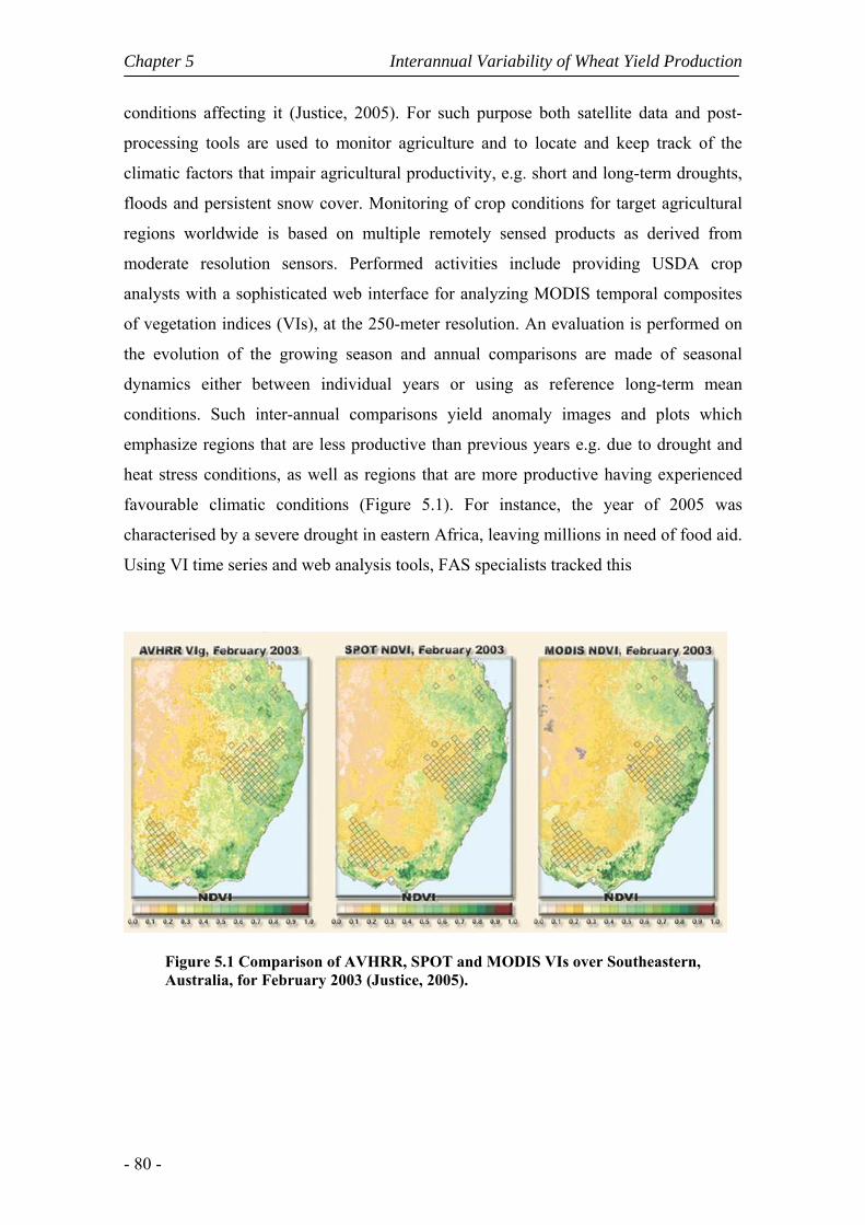
Chapter 5 Interannual Variability of Wheat Yield Production
- 80 -
conditions affecting it (Justice, 2005). For such purpose both satellite data and post-
processing tools are used to monitor agriculture and to locate and keep track of the
climatic factors that impair agricultural productivity, e.g. short and long-term droughts,
floods and persistent snow cover. Monitoring of crop conditions for target agricultural
regions worldwide is based on multiple remotely sensed products as derived from
moderate resolution sensors. Performed activities include providing USDA crop
analysts with a sophisticated web interface for analyzing MODIS temporal composites
of vegetation indices (VIs), at the 250-meter resolution. An evaluation is performed on
the evolution of the growing season and annual comparisons are made of seasonal
dynamics either between individual years or using as reference long-term mean
conditions. Such inter-annual comparisons yield anomaly images and plots which
emphasize regions that are less productive than previous years e.g. due to drought and
heat stress conditions, as well as regions that are more productive having experienced
favourable climatic conditions (Figure 5.1). For instance, the year of 2005 was
characterised by a severe drought in eastern Africa, leaving millions in need of food aid.
Using VI time series and web analysis tools, FAS specialists tracked this
Figure 5.1 Comparison of AVHRR, SPOT and MODIS VIs over Southeastern, Australia, for February 2003 (Justice, 2005).

Interannual Variability of Wheat Yield Production Chapter 5
- 81 -
5.2 Wheat and Climate
During the last decades, the study of weather conditions and of their connection
to plant growth and crop yield has been very important in agricultural research. At the
same time, remote sensing technology has been developing steadily and its products
may provide a large number of applications in agriculture, namely in the cases of crop
identification, crop growth monitoring and yield prediction.
Wheat production and quality are associated with several factors that include
seed variety, soil type and fertilization techniques with the latter being taken as virtually
unvariable over the European Union due to the strict regulations imposed by the
European Community. Nevertheless, climate is still one of the major factors which
influence the spatio-temporal distribution of most agricultural systems, which are
vulnerable to inter-annual climate variability and, in particular, to extreme events and
trends in traditional patterns of regional climate (Hoogenboom, 2000).
Winter atmospheric circulation affects the regional distributions of temperature
and precipitation in Europe and relations have been found between them and wheat
yield for the European countries (Maytelaube et al, 2004); however sensitivity to winter
variability seems to be at the local scale and there is the need to perform a regional
analysis with the aim of clarifying the relationship between winter variability and crops.
Other studies have shown that a high North Atlantic Oscillation (NAO) index in winter
is associated with better quality of the UK wheat crop (Atkinson et al., 2005) and with
better wheat, rye, oat and citrus yields in the Iberian Peninsula (Gimeno et al, 2002).
Estimations of the effects of climate variability on the final crop yields has also been
evaluated at five sites in Spain (Iglesias and Quiroga, 2007) and wheat and barley yields
were predicted in the Ebro valley using drought indices and remote-sensed data
(Vicente-Serrano et al., 2006).
Rodríguez-Puebla et al. (2007) have derived a model able to integrate effects of
climate variables on winter cereals productivity in Spain. The model integrates the
effects of abundant precipitation together with dynamic aspects of the air masses, during
the maturation. The positive effects of warm winters at the beginning of the cereal
growing season were also considered. Several authors have tried to integrate crop
Chapter 5 Interannual Variability of Wheat Yield Production
- 82 -
simulation models with remotely sensed data through data-assimilation methods. This
approach has the advantage of improving initialization of model parameters with
remotely sensed observations to improve model performance (Fang et al., 2008; De
Melo et al., 2008).
The most important meteorological variables associated with agriculture
production are air temperature (daily maximum and minimum values), solar radiation
and precipitation. In particular, solar radiation provides the energy for the processes that
drive photosynthesis (Hoogenboom, 2000) and it has been shown that wheat yields in
Canadian Prairies may be satisfactorily predicted by combining meteorological and
remote sensing data (Boken and Shaykewich, 2002).
5.3 Wheat in Portugal
The majority of wheat in Portugal is sown in October and November and
harvested in June and July of the following year, leading to a small production due to
the existence of a very short vegetative cycle. A comprehensive assessment on the
Portuguese wheat vegetative cycle and the corresponding relationship with climate
variables is given by Sampaio (1990) and Feio (1991).
According to the Köppen’s climate classification, continental Portugal belongs
to the so-called Csa and Csb groups, which are characterized by a typical Mediterranean
climate, with mild and relatively wet winters and dry summers. This situation may be
further worsened by bad drainage of soils. The wheat yield in Portugal is therefore
considerably smaller than the corresponding wheat yield in the North-western European
countries, with cold (but not too wet) winters and relatively wet summers. During the
grain filling until the complete grain ripening phase, the Mediterranean conditions may
even get worse, due to the short period of time between frost episodes and relatively
high temperatures at the end of spring (May/June). Another adverse situation, especially
when compared with the same period for North-western European countries, consists in
the low photoperiod (number of sun hours) and the high temperatures which may occur
at the end of the maturation phase. During this phase large values of potential
evapotranspiration may lead to weak photosynthetic activity, since the plant mostly
spends this activity in the transpiration process in order to fight against the warm season
Interannual Variability of Wheat Yield Production Chapter 5
- 83 -
effects instead of producing dry matter. An excess of evapotranspiration may therefore
lead to a decrease of wheat quality. On the other hand, and as already pointed out, there
is also a strong dependence of wheat yield and quality on temperature, precipitation and
radiation. We will shortly describe the impact of these three meteorological factors on
the vegetative cycle of wheat.
Temperature. Wheat requires low temperature during winter (January/
February), while too high temperature at the end of the cycle may lead to bad
productions. Low temperature and frosts during spring may also cause damages, as
wheat spikes in this season are growing; they are especially sensitive to frost in this
period.
Precipitation. Rainfall is the driving factor of soil moisture, a variable that is
indispensable for the appropriate development of most cultures in Portugal. A good year
for wheat production in Portugal is usually characterized by reasonable precipitation in
late September and early October (in way to prepare the soil to catch-crop), followed by
low precipitation in late autumn and early winter. Moderate precipitation in late winter
and early spring is also beneficial, namely in April, and May. June should be dry, but
not too dry in order to allow for a slow and complete maturation that promotes the
emergence of filled and well formed grains. However intense rain in late June could
favor the development of pests and consequently a decrease on wheat quality. It may be
noted that, in the case of precipitation, the most important issue is the seasonal
distribution throughout the year, not the total annual amount of rainfall. In Portugal this
aspect is generally problematic, due to the irregularity and unpredictability of
precipitation distribution that is typical in Mediterranean climates (Trigo et al., 2004).
Photoperiod (number of sun hours). Radiation has a distinct impact from
temperature in wheat growing. Since solar radiation provides the energy needed to
promote photosynthesis, the number of sunny hours is very important to induce
flowering.
5.3.1 Production and Yield
Wheat yield data for Portugal were extracted from the Food and Agriculture
Organization (FAO) database for the period 1961-2005. Annual averages of wheat yield
in Portugal for the considered period may be observed in Figure 5.2. It may be noticed

Chapter 5 Interannual Variability of Wheat Yield Production
- 84 -
that the yield time series has two components: a trend, due essentially to improvements
in farm management practices and a weather-related yield interannual variability
(Maytelaube et al., 2004). Since our aim is to assess the effects of climate related
variability on crop yield, the “technologically driven” trend was removed from the raw
time series, i.e. we will restrict to annual yield anomalies.
Figure 5.2 Time series of annual wheat yield in Portugal for the period from 1961 to 2005: yield (solid line), general trend (dashed line) and anomalies for detrended time series (line with asterisks).
Data of wheat yield for different regions in Portugal was provided by the
Portuguese Instituto Nacional de Estatísitica (INE) and covers a shorter period from
1996 to 2003; however these data are available for both hard and soft yield wheat. The
main wheat growing area is Alentejo, a region that is located in the southern sector of
Portugal (Figure 5.3). Alentejo contributes with more than 80% of the total wheat
production, and concentrates more than 95% of the total of hard wheat production
(Figure 5.4). It worth stressing that this type of wheat is less sensitive to technological
improvements
Figure 5.3 Contribution of different growing regions of Portugal to total wheat yield for the period from 1996 to 2003.
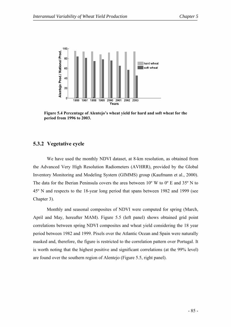
Interannual Variability of Wheat Yield Production Chapter 5
- 85 -
Figure 5.4 Percentage of Alentejo’s wheat yield for hard and soft wheat for the period from 1996 to 2003.
5.3.2 Vegetative cycle
We have used the monthly NDVI dataset, at 8-km resolution, as obtained from
the Advanced Very High Resolution Radiometers (AVHRR), provided by the Global
Inventory Monitoring and Modeling System (GIMMS) group (Kaufmann et al., 2000).
The data for the Iberian Peninsula covers the area between 10º W to 0º E and 35º N to
45º N and respects to the 18-year long period that spans between 1982 and 1999 (see
Chapter 3).
Monthly and seasonal composites of NDVI were computed for spring (March,
April and May, hereafter MAM). Figure 5.5 (left panel) shows obtained grid point
correlations between spring NDVI composites and wheat yield considering the 18 year
period between 1982 and 1999. Pixels over the Atlantic Ocean and Spain were naturally
masked and, therefore, the figure is restricted to the correlation pattern over Portugal. It
is worth noting that the highest positive and significant correlations (at the 99% level)
are found over the southern region of Alentejo (Figure 5.5, right panel).

Chapter 5 Interannual Variability of Wheat Yield Production
- 86 -
Figure 5.5 Patterns of simple correlation between spring NDVI composites and wheat yield in Portugal, for the period of 1982-1999 (left panel); patterns of simple correlation that are significant at the 99% level (right panel).
5.3.3 Spatial distribution
The Corine Land Cover Map (CLC2000), originally on a 250m by 250m grid,
was re-projected to the scale of 8 km by 8km (i.e. the same as in the NDVI database),
using the methodology described in Chapter 3. We have restricted the analysis to the set
of pixels that were coded as non irrigated arable land (Figure 5.6, left panel) and have
then characterized the statistical distribution of correlation coefficient values between
wheat yield and spring NDVI (Figure 5.6, right panel). It is worth noting that the three
higher correlation classes (i.e. those centered at 0.5, 0.7 and 0.9) represent more than
90% of pixels coded as non-irrigated arable land. We have then selected for further
analysis the subset of pixels where correlation values are statistically significant at the
1% level. The subset of selected pixels is shown in Figure 5.7 and it may be noted that
they present a rather homogenous distribution over the south of Alentejo that
corresponds to areas of extensive cultivation of wheat. The considered subset of pixels
will hereafter be referred to as “wheat-like” pixels. We will therefore assess the
statistical significance of the relationship between spring NDVI and wheat yield by
evaluating the correlation between detrended anomalies of wheat yield and averaged
spring NDVI over the selected subset of “wheat-like” pixels.

Interannual Variability of Wheat Yield Production Chapter 5
- 87 -
Figure 5.6 Pixels coded as “arable land not irrigated” according to Corine2000 for Portugal. (left panel). Relative frequency of correlation coefficient values between spring composite of NDVI and wheat yield in Portugal, for pixels coded as arable land (right panel).
Figure 5.7 As in Figure 5.5 (left panel), but for the pixels with correlations that are significant at the 99% level.
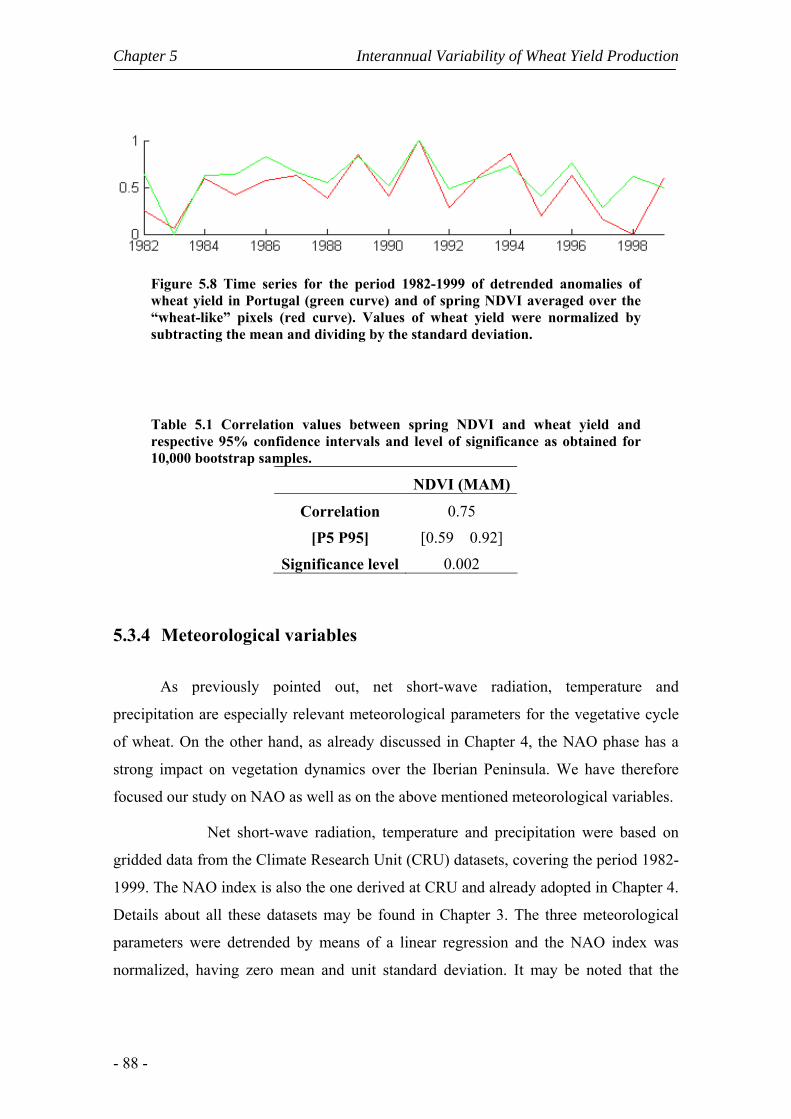
Chapter 5 Interannual Variability of Wheat Yield Production
- 88 -
Figure 5.8 Time series for the period 1982-1999 of detrended anomalies of wheat yield in Portugal (green curve) and of spring NDVI averaged over the “wheat-like” pixels (red curve). Values of wheat yield were normalized by subtracting the mean and dividing by the standard deviation.
Table 5.1 Correlation values between spring NDVI and wheat yield and respective 95% confidence intervals and level of significance as obtained for 10,000 bootstrap samples.
NDVI (MAM)
Correlation 0.75
[P5 P95] [0.59 0.92]
Significance level 0.002
5.3.4 Meteorological variables
As previously pointed out, net short-wave radiation, temperature and
precipitation are especially relevant meteorological parameters for the vegetative cycle
of wheat. On the other hand, as already discussed in Chapter 4, the NAO phase has a
strong impact on vegetation dynamics over the Iberian Peninsula. We have therefore
focused our study on NAO as well as on the above mentioned meteorological variables.
Net short-wave radiation, temperature and precipitation were based on
gridded data from the Climate Research Unit (CRU) datasets, covering the period 1982-
1999. The NAO index is also the one derived at CRU and already adopted in Chapter 4.
Details about all these datasets may be found in Chapter 3. The three meteorological
parameters were detrended by means of a linear regression and the NAO index was
normalized, having zero mean and unit standard deviation. It may be noted that the
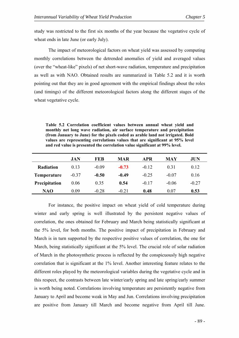
Interannual Variability of Wheat Yield Production Chapter 5
- 89 -
study was restricted to the first six months of the year because the vegetative cycle of
wheat ends in late June (or early July).
The impact of meteorological factors on wheat yield was assessed by computing
monthly correlations between the detrended anomalies of yield and averaged values
(over the “wheat-like” pixels) of net short-wave radiation, temperature and precipitation
as well as with NAO. Obtained results are summarized in Table 5.2 and it is worth
pointing out that they are in good agreement with the empirical findings about the roles
(and timings) of the different meteorological factors along the different stages of the
wheat vegetative cycle.
Table 5.2 Correlation coefficient values between annual wheat yield and monthly net long wave radiation, air surface temperature and precipitation (from January to June) for the pixels coded as arable land not irrigated. Bold values are representing correlations values that are significant at 95% level and red value is presented the correlation value significant at 99% level.
JAN FEB MAR APR MAY JUN
Radiation 0.13 -0.09 -0.73 -0.12 0.31 0.12
Temperature -0.37 -0.50 -0.49 -0.25 -0.07 0.16
Precipitation 0.06 0.35 0.54 -0.17 -0.06 -0.27
NAO 0.09 -0.28 -0.21 0.48 0.07 0.53
For instance, the positive impact on wheat yield of cold temperature during
winter and early spring is well illustrated by the persistent negative values of
correlation, the ones obtained for February and March being statistically significant at
the 5% level, for both months. The positive impact of precipitation in February and
March is in turn supported by the respective positive values of correlation, the one for
March, being statistically significant at the 5% level. The crucial role of solar radiation
of March in the photosynthetic process is reflected by the conspicuously high negative
correlation that is significant at the 1% level. Another interesting feature relates to the
different roles played by the meteorological variables during the vegetative cycle and in
this respect, the contrasts between late winter/early spring and late spring/early summer
is worth being noted. Correlations involving temperature are persistently negative from
January to April and become weak in May and Jun. Correlations involving precipitation
are positive from January till March and become negative from April till June.

Chapter 5 Interannual Variability of Wheat Yield Production
- 90 -
Correlations involving radiation are negative from February until April and become
positive in May and June. Finally, it is worth noting that obtained results are in good
agreement with the recent findings by Rodríguez-Puebla et al. (2007) for Spain.
The described impact of meteorological variables along the vegetative cycle of
wheat is well apparent in Figure 5.9 that presents the monthly patterns of simple
correlations, from January to June, between detrended anomalies of wheat yield and the
three considered meteorological variables.
JAN FEB MAR APR MAY JUN
Figure 5.9 Patterns of simple correlation between wheat yield in Portugal and the three most relevant meteorological fields for the period of 1982-1999; top panel: net short wave radiation; middle panel: surface air temperature; bottom panel: precipitation. Boxes in the Southern sector delimit the area containing “wheat-like” pixels.
Obtained values of correlation between NAO and wheat yield also reflect the
different role played by NAO along the vegetative cycle of wheat. In fact, the contrast
between late winter/early spring and late spring/early summer is well apparent, with
negative correlations between NAO and yield in February and March and positive
correlations in April and June, both statically significant at the 5% level. This behavior
may be viewed as reflecting the integrated impact on radiation, temperature and
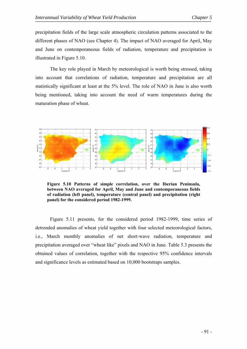
Interannual Variability of Wheat Yield Production Chapter 5
- 91 -
precipitation fields of the large scale atmospheric circulation patterns associated to the
different phases of NAO (see Chapter 4). The impact of NAO averaged for April, May
and June on contemporaneous fields of radiation, temperature and precipitation is
illustrated in Figure 5.10.
The key role played in March by meteorological is worth being stressed, taking
into account that correlations of radiation, temperature and precipitation are all
statistically significant at least at the 5% level. The role of NAO in June is also worth
being mentioned, taking into account the need of warm temperatures during the
maturation phase of wheat.
Figure 5.10 Patterns of simple correlation, over the Iberian Peninsula, between NAO averaged for April, May and June and contemporaneous fields of radiation (left panel), temperature (central panel) and precipitation (right panel) for the considered period 1982-1999.
Figure 5.11 presents, for the considered period 1982-1999, time series of
detrended anomalies of wheat yield together with four selected meteorological factors,
i.e., March monthly anomalies of net short-wave radiation, temperature and
precipitation averaged over “wheat like” pixels and NAO in June. Table 5.3 presents the
obtained values of correlation, together with the respective 95% confidence intervals
and significance levels as estimated based on 10,000 bootstraps samples.

Chapter 5 Interannual Variability of Wheat Yield Production
- 92 -
Figure 5.11 Patterns of simple correlation between wheat yield in Portugal and the three most relevant meteorological fields for the period of 1982-1999; top panel: net long wave radiation; middle panel: surface air temperature; bottom panel: precipitation.
Table 5.3 As in Table 5.1, but respecting to net short-wave radiation, temperature, precipitation in March and to NAO in June.
Radiation
(MAR)
Temperature
(MAR)
Precipitation
(MAR)
NAO
(JUN)
Correlation -0.73 -0.49 0.54 0.53
[P5 P95] [-0.88 -0.52] [-0.78 -0.13] [0.18 0.80] [0.23 0.78]
Significance level 0.0006 0.04 0.02 0.03
Interannual Variability of Wheat Yield Production Chapter 5
- 93 -
5.4 A simple regression model for wheat yield
Results obtained in the previous section suggest using spring NDVI together
with meteorological variables to build up a simple model of wheat yield in Portugal for
the period 1982-1999. We have accordingly tried several regression models that used as
predictors spring NDVI combined with the meteorological factors shown in Table 5.3.
Statistical models developed with relatively short time series are particularly prone to
overfitting problems (Wilks, 1995), to solve this caveat it is advisable to apply cross
validation techniques, i.e to split the available time series in a calibration and validation
periods. Evaluation of model performance and prevention of overfitting was done by
means of leave-one-out cross validation technique i.e., by using a single observation
from the original sample as the validation data, and the remaining observations as the
training data
Best results were obtained when using as predictors spring NDVI together with
the NAO for June. The best performance of this model may be viewed as reflecting the
fact that chosen predictors grasp the relevant information during two crucial stages for
wheat; the growing and the mature stages. Spring NDVI is an indicator of the
healthiness of wheat during the growing stage which in turn reflects the meteorological
conditions in terms of radiation, temperature and precipitation regimes. On the other
hand NAO for June is an indicator of the large-scale circulation affecting Portugal
which in turn is related to regional conditions in terms of radiation, temperature and
precipitation that have an important role in the process of maturation of wheat.
Figure 5.12 (upper panel) presents, for the considered period 1982-1999, the
time series of observed and modeled wheat yield. The overall agreement is worth being
noted, the two time-series presenting a correlation of 0.83.
Figure 5.12 (central panel) shows the time series of residuals, defined as
departures of observed values from modeled ones. The 95% confidence intervals
relative to these residuals (Chatterjee and Hadi, 1986) are plotted as error bars and it
may be noted that 1998 represents the single outlier since its error bar does not cross the
zero reference line.
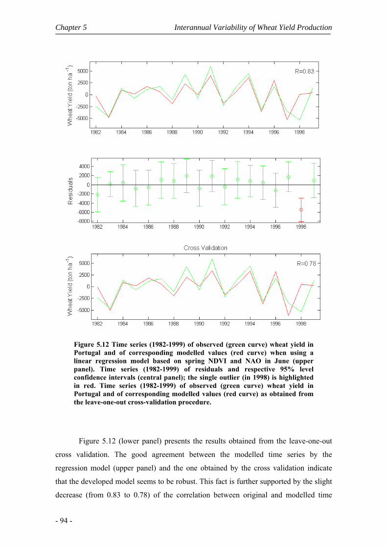
Chapter 5 Interannual Variability of Wheat Yield Production
- 94 -
Figure 5.12 Time series (1982-1999) of observed (green curve) wheat yield in Portugal and of corresponding modelled values (red curve) when using a linear regression model based on spring NDVI and NAO in June (upper panel). Time series (1982-1999) of residuals and respective 95% level confidence intervals (central panel); the single outlier (in 1998) is highlighted in red. Time series (1982-1999) of observed (green curve) wheat yield in Portugal and of corresponding modelled values (red curve) as obtained from the leave-one-out cross-validation procedure.
Figure 5.12 (lower panel) presents the results obtained from the leave-one-out
cross validation. The good agreement between the modelled time series by the
regression model (upper panel) and the one obtained by the cross validation indicate
that the developed model seems to be robust. This fact is further supported by the slight
decrease (from 0.83 to 0.78) of the correlation between original and modelled time

Interannual Variability of Wheat Yield Production Chapter 5
- 95 -
series. However results of the model should be regarded with some caution, given the
short length of the analyzed time series (18 years).
5.5 Final Remarks
We have computed point correlations between spring NDVI over Portugal and
wheat yield during the period 1982-1999. We have found strongly negative correlations
(statistically significant at the 1% level) over Southern Portugal (Alentejo), a region
where more than 80% of wheat is produced and more than 95% of the total of hard
wheat production is concentrated. We have then selected the so-called subset of “wheat-
like” pixels, i.e. pixels coded as non-irrigated arable land associated to correlation
values that are statistically significant at the 1% level.
The impact of meteorological factors on wheat yield was assessed by computing
monthly correlations of the detrended anomalies of yield with averaged values (over the
“wheat-like” pixels) of net short-wave radiation, temperature and precipitation as well
as with NAO. Obtained results are in good agreement with the empirical findings about
the roles (and timings) of the different meteorological factors along the different stages
of the wheat vegetative cycle. In particular, cold temperatures during winter and early
spring, precipitation in February and March and solar radiation in March have a positive
impact during the growing stage, whereas a larger NAO index in July is beneficial for
the maturation stage.
A regression model was finally built up using as predictors spring NDVI and
NAO in June. Performance of the model was quite satisfactory, with a generally good
agreement between observed and modelled wheat yield. Although results may still be
considered as preliminary, given the short length of the analyzed series (18 years), the
model is expected to be useful to for wheat yield monitoring. The model is also
expected to be improved when extending it to an enlarged GIMMS dataset (1982-2006).

6. DROUGHT AND VEGETATION STRESS
MONITORING
6.1 Introduction
The Iberian Peninsula is recurrently affected by drought episodes and by the
adverse effects associated that range from severe water shortages to economic losses
and related social impacts. For instance, during the hydrological year of 2004/2005, the
Iberian Peninsula was hit by one of the two worst drought episodes that were recorded
in the last six decades (Garcia-Herrera et al., 2007), reinforcing the need for a
continuous monitoring of vegetation stress and for reliable estimates of the drought
impacts. In this respect it is worth mentioning that more than 280 M€ were spent in
order to compensate for the damage associated with the 2005 drought in continental
Portugal (MADRP, 2005).
The strong dependence of vegetation dynamics on water availability has been for
long recognized in the Mediterranean and other semi-arid regions (Eagleson, 2002,
Rodríguez-Iturbe and Porporato, 2004, Vicente-Serrano and Heredia-Laclaustra, 2004,
Vicente-Serrano, 2007). A combined effect of lack of precipitation over a certain period
with other climatic anomalies, such as high temperature, high wind and low relative
humidity over a particular area may result in reduced green vegetation cover. When
drought conditions end, recover of vegetation may follow (Nicholson et al., 1998) but
the process may last for longer periods of time (Diouf and Lambin, 2001).
Traditional methods of drought assessment and monitoring depend heavily on
rainfall data as recorded in meteorological and hydrological networks. However the
availability of reliable satellite imagery covering wide regions over long periods of time
has progressively strengthen the role of remote sensing in environmental studies, in
particular in those related to drought episodes (Kogan, 1995, 1997, 2000, Kogan et al.,
2004, McVicar and Jupp, 1998, 1999, 2002). Drought early warning and monitoring are

Chapter 6 Drought and Vegetation Stress Monitoring
- 98 -
crucial components of drought awareness and mitigation plans (Wilhite, 1993) and it is
worth stressing, that with the help from environmental satellites, drought can be
detected 4-6 weeks earlier than before and delineated more accurately (Kogan, 2000).
In recent years there has been a considerable amount of drought studies dealing
with different regions of Europe as well as covering the entire European continent
(Briffa et al., 1994; Gibb et al., 1978; Marsh and Lees, 1985; Phillips and McGregor,
1998; Bussay et al., 1999; Estrela et al., 2000; Lana et al., 2001; Lloyd-Hughes and
Saunders, 2002). Summer droughts are the most important in terms of human
perception, but water shortages during the other seasons may also have significant
socio-economic impacts (EEA, 2001). Several authors have examined the special case
of the Iberian Peninsula (Garcia-Herrera et al., 2007, Vicente-Serrano, 2006) and it may
be noted that, even though the recent 2005 drought has been ranked among the strongest
ones of the last century in Portugal, the episodes of 1945, 1981, 1983, 1992 and 1999
were also major events (Feio and Henriques, 1986; Godinho et al., 1992). In addition, a
slight downward trend has been found in the annual precipitation recorded over
Portugal (Zhang et al., 1997, Miranda et al., 2006) that is particularly noticeable in early
spring (Trigo and DaCamara, 2000, Garcia-Herrera et al., 2007). However, less
attention has been paid to the impacts of drought in vegetation activity as well as to the
sensitivity of the photosynthetic mechanisms to water stress.
The aim of the present chapter is therefore to make use of remote-sensed
information in order to monitor the spatial and temporal distribution of heat and water
stress of vegetation in Continental Portugal. The severity of a given drought episode
will then be assessed by evaluating the cumulative impact over time of heat and water
stress conditions on vegetation in a certain region. Special attention will be devoted to
the above mentioned extreme drought episode of 2005, as well as to those of 1999 and
2002. It may be noted that the latter episode has mainly affected Northeastern Portugal
in strong contrast with the other two episodes that have struck hardest Southern
Portugal.

Drought and Vegetation Stress Monitoring Chapter 6
- 99 -
6.2 Vegetation stress
The response of vegetation to heat and water stress was assessed based on fields
of NDVI as derived from the VEGETATION instrument on-board SPOT5. As
discussed in Chapter 3, any vegetation monitoring based on NDVI requires a previous
correction of the time-series, in order to distinguish real changes in the annual cycles of
vegetation greenness from those due other factors, e.g. contamination by clouds,
shadows and snow and sun/view directional dependence of spectral response. Figure 6.1
presents monthly values of NDVI that were spatially averaged over Continental
Portugal. The years of 1999, 2002 and 2005 are conspicuous because of the occurrence
of low values of vegetation greenness, especially during the growing season, i.e., during
the period of high photosynthetic activity. In the case of the droughts of 1999 and 2005,
this is especially apparent when the spatial averages are performed over non-irrigated
arable land, a feature that is in contrast with the case of 2002 where the lower values are
well visible over broad-leaved forest. The delay of the growing season of arable land
together with the observed relative insensitivity in the case of broad-leaved forest is
another interesting feature that suggests drought conditions to be responsible for both
delaying and shortening the growing season.
Figure 6.1 Monthly time-series (1999–2006) of NDVI averaged over Continental Portugal for all pixels (black line), for pixels of non-irrigated arable land (red line) and of pixels of broad-leaved forest (green line). Black arrows indicate the drought episodes of 1999, 2002 and 2005.

Chapter 6 Drought and Vegetation Stress Monitoring
- 100 -
Figure 6.2 Monthly means of NDVI (1999-2006) over Continental Portugal, covering the period from September to August.

Drought and Vegetation Stress Monitoring Chapter 6
- 101 -
Figure 6.2 presents the monthly mean fields of NDVI from September to August,
over Continental Portugal and covering the period 1999-2006. As expected, larger
values of NDVI associated with an increase in photosynthetic activity, and therefore in
vegetation greenness, may be found in winter and spring over Southern Portugal.
During summer and autumn this region presents low values, a feature that is coherent
with the vegetation types of a semi-arid environment. In contrast, Northwestern
Portugal presents high values of vegetation greenness as expected from the presence of
forest, the predominant vegetation cover.
6.3 Drought assessment
6.3.1 Annual cycle of NDVI
Figures 6.3 to 6.5 show monthly anomaly fields of NDVI from September to
August, respectively for the years 1998/1999, 2001/2002 and 2004/2005. It may be
noted that monthly anomalies of a given month are defined as departures from the
median of that month (computed over the considered period 1999-2006). Usage of the
median (instead of the mean) was made in order to avoid the lever effect by the
extremely low NDVI values that were attained in the droughts years, taking into
account the small length of the sample (8 years).
As already discussed, the three chosen drought years are characterised by low
vegetation greenness activity associated to low values of NDVI (Figure 6.1). In the case
of 1999 (Figure 6.3) the highest negative anomalies (around -0.30) present an early start
in November and persistently remain until April. The most affected regions are located
in Southern Portugal and it may be noted that the impact of the drought is apparent until
May. A strong contrast in the spatial distribution may be observed in the case of 2002
(Figure 6.4) the highest negative anomalies being mainly located over Northeastern
Portugal where negative values (around -0.10) may be found extending from November
to February. During 2005 (Figure 6.5), the highest negative anomalies (around -0.30)
may be observed, over Southern Portugal, between February and June.

Chapter 6 Drought and Vegetation Stress Monitoring
- 102 -
Figure 6.3 NDVI anomalies from September to August respecting to the year of 1998/1999.

Drought and Vegetation Stress Monitoring Chapter 6
- 103 -
Figure 6.4 As in Figure 6.3 but respecting to the year of 2001/2002.

Chapter 6 Drought and Vegetation Stress Monitoring
- 104 -
Figure 6.5 As in Figure 6.3 but respecting to the year of 2004/2005.

Drought and Vegetation Stress Monitoring Chapter 6
- 105 -
It is worth emphasising that, in the cases of the 1999 and 2005 drought episodes,
the area of stressed vegetation is located in the south of Portugal, a region that is
generally covered by non-irrigated arable land (Figure 3.9) with semi-arid
characteristics and presenting a strong desertification risk. It may be further noted that
the location of stressed pixels is also in good agreement with the results of Vicente-
Serrano (2006) who has shown that the impact of climate variability and associated
extreme events (such as drought) on vegetation activity is most pronounced over most
arid areas. Finally, in the case of the 2005 drought episode, it is worth stressing that the
observed negative anomalies are contemporaneous with the period of high
photosynthetic activity (i.e., high NDVI values in Figure 6.2), leading to a further
amplification of the negative impact on vegetation dynamics and therefore to an even
larger drought impact.
6.3.2 Annual cycle of soil moisture
Since a quick response of vegetation to spatio-temporal variations in soil moisture
is generally observed in semi-arid regions (Bonifacio et al., 1993; Sannier and Taylor,
1998), the impact of soil moisture on vegetation dynamics is worth being analysed. We
have relied on the Global Soil Moisture Archive (http://www.ipf.tuwien.ac.at/radar/ers-
scat/home.htm) for the period 1992-2005 (Scipal, 2002) and have extracted the so-
called Soil Water Index (SWI) which is based on the method developed by Wagner et
al. (1999a, b). The archive is based on information from the European Remote Sensing
(ERS) Scatterometer instrument on-board ERS-1 and ERS-2 satellites, operated by the
European Space Agency (ESA), which achieve global coverage within 3 to 4 days with
a 25 km grid spacing. SWI fields were interpolated to a 0.25º latitude-longitude grid
covering the same window that was defined for NDVI (see Chapter 3).
Figure 6.6 presents spatially averaged values over Portugal of SWI and it is well
apparent that the drought episodes of 1999 and 2005 are characterised by an annual
cycle reaching values well below the remaining years. Figure 6.7 presents the monthly
mean fields of SWI from September to August, over Continental Portugal and covering
the same period. The annual cycle of soil moisture is well apparent and the contrast

Chapter 6 Drought and Vegetation Stress Monitoring
- 106 -
between the regions North and South of the Tagus valley is worth being noted in the
transition seasons.
Figure 6.6 Monthly time-series (1992–2005) of SWI averaged over Continental Portugal. Values from January 2001 until August 2003 are missing. Black arrows indicate the drought episodes of 1999 and 2005.
The response of vegetation to soil moisture is well illustrated in Figure 6.8 that
presents the annual cycle of SWI vs. NDVI as obtained from averaging the periods of
study. The initial linear relationship between NDVI and SWI from August to December
translates the contemporaneous response of vegetation to soil moisture that leads to a
maximum of greenness in January. However, the following period presents a non linear
behaviour. The strong decrease in SWI between January and April corresponds to a
slight decrease of NDVI, suggesting that vegetation greenness is sustained by the
cumulated soil water during winter time. A contemporaneous response of NDVI to SWI
is again observed from April to August, closing the vegetation cycle.
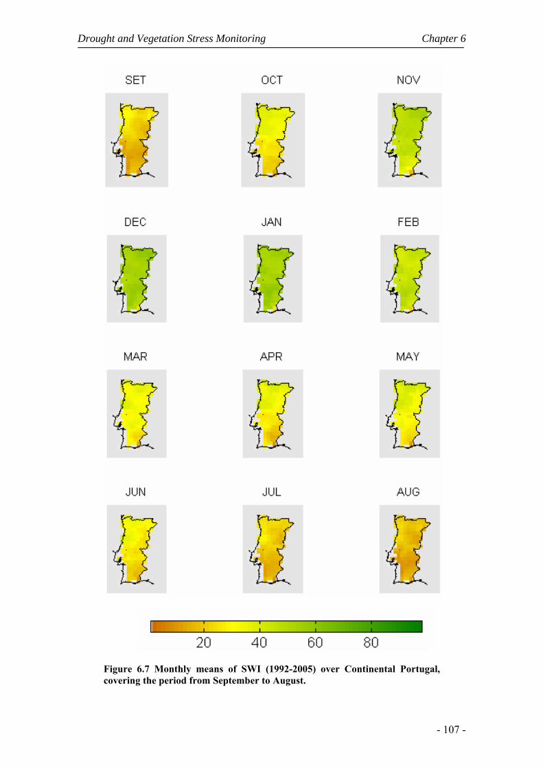
Drought and Vegetation Stress Monitoring Chapter 6
- 107 -
Figure 6.7 Monthly means of SWI (1992-2005) over Continental Portugal, covering the period from September to August.

Chapter 6 Drought and Vegetation Stress Monitoring
- 108 -
Figure 6.8 Climatological cycle of SWI vs. NDVI. Letters indicate months of the year.
Figures 6.9 and 6.10 present the spatial distribution over Continental Portugal of
monthly anomalies of SWI for the drought episodes of 1999 and 2005. The drought
episode of 2002 was not considered because of the unavailability of SWI data for the
year 2001/2002. SWI anomalies are defined as departures from the mean of the
respective month over the considered 14-year period (1992-2005) and as opposed to the
drought episode of 2005, where the occurrence of negative anomaly values of SWI only
begin in spring, drought conditions start to occur in the beginning of winter 1998/1999.

Drought and Vegetation Stress Monitoring Chapter 6
- 109 -
Figure 6.9 SWI anomalies for January to August respecting to the year 1998/1999.
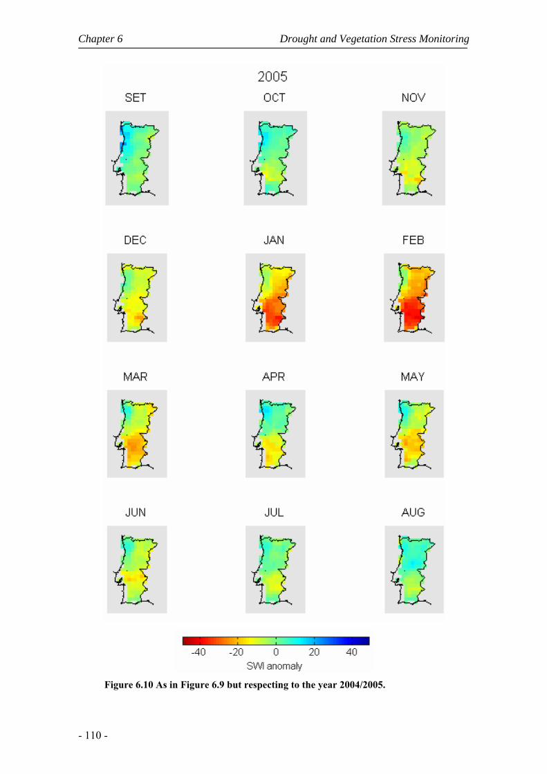
Chapter 6 Drought and Vegetation Stress Monitoring
- 110 -
Figure 6.10 As in Figure 6.9 but respecting to the year 2004/2005.
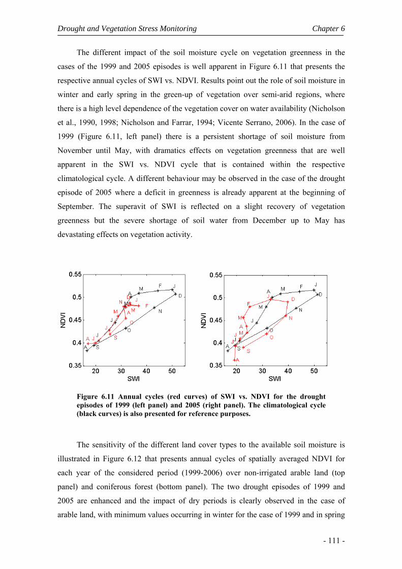
Drought and Vegetation Stress Monitoring Chapter 6
- 111 -
The different impact of the soil moisture cycle on vegetation greenness in the
cases of the 1999 and 2005 episodes is well apparent in Figure 6.11 that presents the
respective annual cycles of SWI vs. NDVI. Results point out the role of soil moisture in
winter and early spring in the green-up of vegetation over semi-arid regions, where
there is a high level dependence of the vegetation cover on water availability (Nicholson
et al., 1990, 1998; Nicholson and Farrar, 1994; Vicente Serrano, 2006). In the case of
1999 (Figure 6.11, left panel) there is a persistent shortage of soil moisture from
November until May, with dramatics effects on vegetation greenness that are well
apparent in the SWI vs. NDVI cycle that is contained within the respective
climatological cycle. A different behaviour may be observed in the case of the drought
episode of 2005 where a deficit in greenness is already apparent at the beginning of
September. The superavit of SWI is reflected on a slight recovery of vegetation
greenness but the severe shortage of soil water from December up to May has
devastating effects on vegetation activity.
Figure 6.11 Annual cycles (red curves) of SWI vs. NDVI for the drought episodes of 1999 (left panel) and 2005 (right panel). The climatological cycle (black curves) is also presented for reference purposes.
The sensitivity of the different land cover types to the available soil moisture is
illustrated in Figure 6.12 that presents annual cycles of spatially averaged NDVI for
each year of the considered period (1999-2006) over non-irrigated arable land (top
panel) and coniferous forest (bottom panel). The two drought episodes of 1999 and
2005 are enhanced and the impact of dry periods is clearly observed in the case of
arable land, with minimum values occurring in winter for the case of 1999 and in spring

Chapter 6 Drought and Vegetation Stress Monitoring
- 112 -
for the case of 2005. However, over coniferous forests, lower than average values of
NDVI may still be observed during the beginning of winter in the case of 1999 and
during spring in the case of 2005.
Figure 6.12 Annual cycles of spatially averaged NDVI for each year of the considered period (1999-2006) over non-irrigated arable land (top panel) and coniferous forest (bottom panel). The drought episodes of 1999 and 2005 are represented, respectively, by the curves with circles and asterisks. The line in bold refers to monthly means over the entire period.
6.4 Drought persistence
The severity of a given drought episode is often assessed by means of the so
called Palmer Drought Severity Index (PDSI) that is based on a supply-and-demand
model of soil moisture (Palmer, 1965). The aim of PDSI is to provide standardized
measurements of moisture conditions so that comparisons can be made between
locations and between months.
Based on the concept of water balance, PDSI is mainly a meteorological index
which responds to weather conditions that have been unusually dry or unusually wet.
Drought and Vegetation Stress Monitoring Chapter 6
- 113 -
Details on the evaluation of PDSI, as well as about its usefulness and limitations, may
be found e.g., in Alley (1984). The index is usually computed on a monthly basis and
has proven as especially adequate to characterise long-term droughts. Values of PDSI,
which roughly vary between -6.0 and +6.0 are derived from the following relationship
10.8973
ii i
ZX X −= + (6.1)
where Xi and Zi respectively denote the monthly values for month i of PDSI and the so-
called moisture anomaly index which takes into account the difference between the
actual precipitation in month i and the amount of precipitation that is “climatologically
appropriate” for the existing conditions, weighted by a “climate characteristic”, K
(Palmer, 1965). Since the first term of the equation (6.1) introduces an autoregressive
process, PDSI has a certain length of memory (Karl, 1986).
Drought episodes are associated to negative values of PDSI and are usually
grouped into the so-called drought severity classes which are defined as follows;
moderate drought (PDSI ≈ -2), severe drought (PDSI ≈ -3) and extreme drought (PDSI
≈ -4).
Figure 6.13 presents, for the year of 2004/2005, the evolution on a monthly basis
(black curve) of the percentage of continental Portugal that is under extreme drought
conditions according to WMO (2006). The respective evolution of the percentage of the
territory with stressed (red bars) and very stressed (green bars) vegetation is also shown
in the figure. It may be noted that the area of stressed (very stressed) vegetation was
estimated based on the fraction of pixels with anomalies lower than 0 (lower than -
0.025). The severity of the drought episode of 2005 is well apparent taking for instance
into account that, in May, almost 90% of continental Portugal is covered by pixels with
NDVI anomalies lower than 0.
Figure 6.13 also shows the existence of a delay of about three months of PDSI
relatively to NDVI. This delay, that is especially visible for very stressed vegetation,
translates the above mentioned memory of PDSI. Moreover, the observed good
agreement, for the 2005 drought episode, between the percentage of territory affected by
extreme drought and associated to very stressed vegetation suggests adopting a
threshold of -0.025 to identify pixels affected by drought conditions in the remaining
years of the study period.

Chapter 6 Drought and Vegetation Stress Monitoring
- 114 -
Figure 6.13 Percentage of continental Portugal with monthly NDVI anomalies lower than 0 (red bars) and lower than -0.025 (green bars), from September to August of 2005. The black line represents the percentage of mainland affected by extreme drought, i.e., with PDSI ≈ -4. The 3-month delay of PDSI relatively to NDVI (as indicated by the two different horizontal time axes) is worth being noted.
As mentioned above, an important aspect to be considered when assessing
drought severity respects to the persistence of dry conditions for a given location.
Accordingly, we have evaluated drought persistence by simply counting, for each pixel,
the number of months with NDVI anomalies lower than -0.025. Results are shown in
Figure 6.14 and the years of 1999, 2002 and 2005 are particularly striking due to the
large areas affected by persistent drought. In the cases of the drought episodes of 1999
and 2005, pixels located over the south of Portugal reveal up to nine months (out of
eleven) of persistently stressed vegetation. In the case of the drought episode of 2002 a
considerable vast area over Noutheastern Portugal presents more than eight months (out
of eleven) of stressed vegetation.
Table 6.1 presents the percentage of mainland Portugal stricken by serious
drought, i.e., with monthly NDVI anomalies below -0.025 in more than 9 months (out
of 11). The exceptionality of 2005 is again conspicuous, with more than one third of
Portugal with more than 9 months in vegetation stress, an area that is twice the one
observed in 1999. The amount of 11% of mainland affected in the case of 2002 is still
contrasting with the remaining years of the considered period.
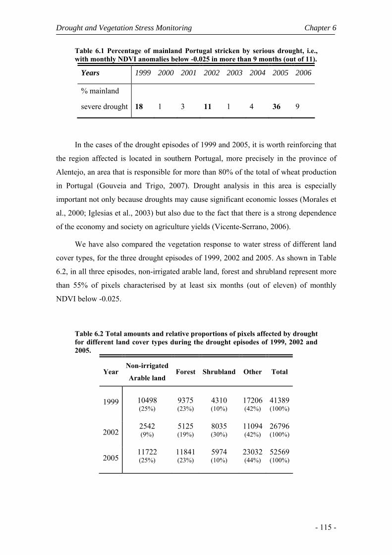
Drought and Vegetation Stress Monitoring Chapter 6
- 115 -
Table 6.1 Percentage of mainland Portugal stricken by serious drought, i.e., with monthly NDVI anomalies below -0.025 in more than 9 months (out of 11).
Years 1999 2000 2001 2002 2003 2004 2005 2006
% mainland
severe drought
18
1
3
11
1
4
36
9
In the cases of the drought episodes of 1999 and 2005, it is worth reinforcing that
the region affected is located in southern Portugal, more precisely in the province of
Alentejo, an area that is responsible for more than 80% of the total of wheat production
in Portugal (Gouveia and Trigo, 2007). Drought analysis in this area is especially
important not only because droughts may cause significant economic losses (Morales et
al., 2000; Iglesias et al., 2003) but also due to the fact that there is a strong dependence
of the economy and society on agriculture yields (Vicente-Serrano, 2006).
We have also compared the vegetation response to water stress of different land
cover types, for the three drought episodes of 1999, 2002 and 2005. As shown in Table
6.2, in all three episodes, non-irrigated arable land, forest and shrubland represent more
than 55% of pixels characterised by at least six months (out of eleven) of monthly
NDVI below -0.025.
Table 6.2 Total amounts and relative proportions of pixels affected by drought for different land cover types during the drought episodes of 1999, 2002 and 2005.
Year Non-irrigated
Arable land Forest Shrubland Other Total
1999
10498 (25%)
9375 (23%)
4310 (10%)
17206(42%)
41389 (100%)
20022542 (9%)
5125 (19%)
8035 (30%)
11094(42%)
26796 (100%)
200511722 (25%)
11841(23%)
5974 (10%)
23032(44%)
52569 (100%)

Figure 6.14 Number of months between September and August that are characterised by NDVI anomaly values below -0.025, for each year of the considered period (1999-2006).
Drought and Vegetation Stress Monitoring Chapter 6
-117-
As expected the episode of 2005 ranks first in what respects to the total amount of
affected pixels (52569), followed by 1999 (41389) and 2002 (26796). However there
are interesting differences when comparing the drought episodes of 1999 and 2005
versus the episode of 2002 in what respects to the proportion of affected vegetation
types. Arable land was especially affected during the 1999 and 2005 episodes, whereas
shrubland was the most affected land cover type during the 2002 episode. Forest was
affected in similar proportions during the three drought episodes and the remaining
types of vegetation do not show as well noticeable differences among episodes.
The cumulative effect of drought conditions on the three considered types of
vegetation was further investigated by analysing the relative proportions of pixels that
remained with monthly anomalies of NDVI below -0.025 for 7, 8 and 9 months. Results
are presented in Table 6.3 and conspicuous differences may be found among the three
drought episodes. The exceptional strength of the drought episode of 2005 is well
illustrated by the percentage of affected pixels of all vegetation types (including forest),
with more than half of the pixels being affected for more than 9 months. In the case of
the drought episode of 1999 non-irrigated arable land was the main vegetation type
affected, with a total amount of almost one third of the pixels being affected for more
than 9 months. Finally, in the case of the episode of 2002, shrubland was the most
affected vegetation type with slightly more than one third being affected for at least 9
months.

Chapter 6 Drought and Vegetation Stress Monitoring
- 118 -
Table 6.3 Cumulative effect of drought conditions for specific land cover types during the drought episodes of 1999, 2002 and 2005.
Nº Months Non-irrigated
Arable land Forest Shrubland
1999
≥ 6 100 100 100
≥ 7 87 76 74
≥ 8 64 47 43
≥ 9 31 17 18
2002
≥ 6 100 100 100
≥ 7 72 66 74
≥ 8 48 43 53
≥ 9 29 26 34
2005
≥ 6 100 100 100
≥ 7 93 85 83
≥ 8 83 71 66
≥ 9 65 54 50
6.5 Final remarks
An assessment was made on the potential usage of environmental satellites for the
detection and monitoring of drought events in Continental Portugal. For this purpose,
annual cycles of vegetation greenness were analysed by examining, for each year, the
monthly anomalies of NDVI. Special attention was devoted to the years of 1999, 2002
and 2005 because of the occurrence of low values of vegetation greenness during the
growing season. In the case of the drought episodes of 1999 and 2005, southern
Portugal was mostly affected, whereas in the case of 2002 the highest negative
anomalies were mostly located in Northern Portugal.
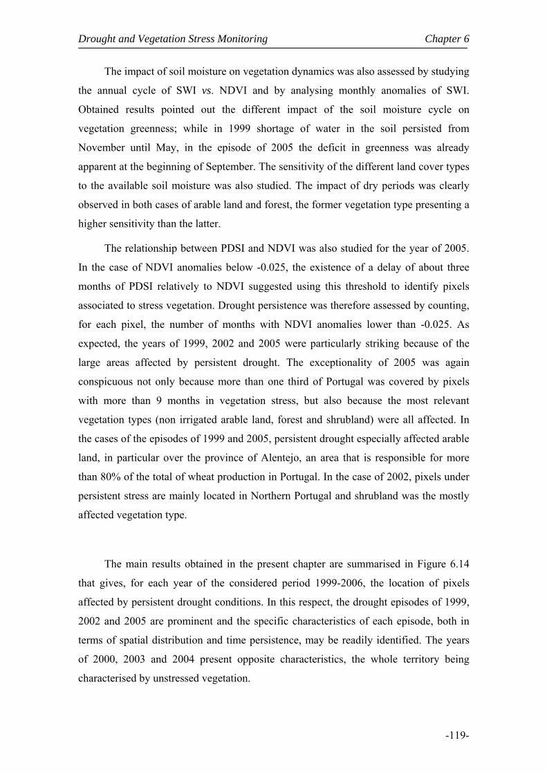
Drought and Vegetation Stress Monitoring Chapter 6
-119-
The impact of soil moisture on vegetation dynamics was also assessed by studying
the annual cycle of SWI vs. NDVI and by analysing monthly anomalies of SWI.
Obtained results pointed out the different impact of the soil moisture cycle on
vegetation greenness; while in 1999 shortage of water in the soil persisted from
November until May, in the episode of 2005 the deficit in greenness was already
apparent at the beginning of September. The sensitivity of the different land cover types
to the available soil moisture was also studied. The impact of dry periods was clearly
observed in both cases of arable land and forest, the former vegetation type presenting a
higher sensitivity than the latter.
The relationship between PDSI and NDVI was also studied for the year of 2005.
In the case of NDVI anomalies below -0.025, the existence of a delay of about three
months of PDSI relatively to NDVI suggested using this threshold to identify pixels
associated to stress vegetation. Drought persistence was therefore assessed by counting,
for each pixel, the number of months with NDVI anomalies lower than -0.025. As
expected, the years of 1999, 2002 and 2005 were particularly striking because of the
large areas affected by persistent drought. The exceptionality of 2005 was again
conspicuous not only because more than one third of Portugal was covered by pixels
with more than 9 months in vegetation stress, but also because the most relevant
vegetation types (non irrigated arable land, forest and shrubland) were all affected. In
the cases of the episodes of 1999 and 2005, persistent drought especially affected arable
land, in particular over the province of Alentejo, an area that is responsible for more
than 80% of the total of wheat production in Portugal. In the case of 2002, pixels under
persistent stress are mainly located in Northern Portugal and shrubland was the mostly
affected vegetation type.
The main results obtained in the present chapter are summarised in Figure 6.14
that gives, for each year of the considered period 1999-2006, the location of pixels
affected by persistent drought conditions. In this respect, the drought episodes of 1999,
2002 and 2005 are prominent and the specific characteristics of each episode, both in
terms of spatial distribution and time persistence, may be readily identified. The years
of 2000, 2003 and 2004 present opposite characteristics, the whole territory being
characterised by unstressed vegetation.

Chapter 6 Drought and Vegetation Stress Monitoring
- 120 -
However a closer look to the year of 2004 reveals an unexpected behaviour. In
fact two well defined regions, respectively, located in Central Portugal and in the
Southwest, show a deep contrast with the background, the pixels presenting monthly
anomalies below -0.025 for 9 to up 11 months. Such a behaviour is not compatible with
the one associated to drought conditions. In fact, a comparison with a map of fire scars
respecting to the summer season of 2003 could immediately lead to the identification of
the two areas as representing the signature of wildfires that occurred in the previous
year.
This feature is especially interesting because it raises the possibility of adapting
the developed technique to identify burned areas and to assess the recovery of
vegetation over areas stricken by fire. Figure 6.15 is an updated version of Figure 6.14,
where we have masked all pixels that were identifying as burned areas using the
procedure described in Chapter 7, that is dedicated to the problem of burned area
monitoring and vegetation recovery.
Figure 6.15 As in Figure 6.14, but all pixels that are identify as burned areas are masked


7. MONITORING BURNED AREAS AND VEGETATION
RECOVERY
7.1 Introduction
The number of fires and the extent of the burned surface in Mediterranean Europe
have strongly increased during the last decades. This may be due either to land-use
changes (e.g. land abandonment and fuel accumulation) or to climatic changes (e.g.
reduction of fuel humidity) that increase fire risk and fire spread (Pausas and Vallejo,
1999). As in the Mediterranean ecosystems, fires in Portugal have an intricate effect on
vegetation regeneration due to the complexity of landscape structures as well as to the
different responses of vegetation to the variety of fire regimes (Wittenberg et al., 2006).
Vegetation cover has, in turn, a key role on soil erosion and land degradation processes
(Shakesby et al., 1993). For instance, the destruction of vegetation by wildfires
generally leads to an intensification of runoff and erosive processes (Inbar et al., 1997;
1998). Thornes (1990) has suggested that a minimum of 30% in vegetation cover is
required to protect the soils against water erosion. Studies performed at various spatial
scales and under different ecological conditions indicate that the majority of loss of
sediments occurs during the first year after fire occurrence (DeBano et al., 1998, Inbar
et al., 1998 and Cerda and Doerr, 2005) and that the risk of post-fire soil erosion
increases with the time required for vegetation to reach the minimal threshold cover
(Shakesby et al., 1993; Inbar et al., 1998; Cerda, 1998a; Cerda, 1998b). A thorough
evaluation of vegetation recovery after fire events becomes therefore crucial in land
management (Wittenberg et al., 2006).
In the above mentioned context remote sensing plays an important role because it
has revealed to be particularly useful to estimate post-fire vegetation dynamics. A
Chapter 7 Monitoring Burned Areas and Vegetation Recovery
- 124 -
considerable number of fire recovery studies based on remote sensing have been
conducted in regions characterised by Mediterranean climates (Jakubauskas et al., 1990;
Marchetti et al., 1995; Viedma et al., 1997; Díaz-Delgado et al., 1998; Henry and Hope,
1998; Ricotta et al., 1998). Several authors have also tested the use of NDVI to monitor
plant regeneration after fire (Malingreau et al., 1985; Paltridge and Barber, 1988;
Viedma et al., 1997; Illera et al., 1996). It may be noted, however, that satellite data are
not adequate to accurately detect high resolution changes in the structure of vegetation.
Several studies have shown that rapid regeneration occurs within the first 2 years
after the fire occurrences (Trabaud, 1981; Kutiel, 1994; Inbar et al., 1998), with distinct
recovery rates at the north and the south facing slopes (Cerda and Doerr, 2005). Pausas
and Vallejo (1999) have shown that, in the Iberian Peninsula, one year after a single fire
event vegetation cover reached 52% on the north facing slope and 32% on the south
facing slope. Similar trends were found at the Mt. Carmel region, Israel, after the 1988
fire event (Kutiel, 1994; Inbar et al., 1998). Díaz-Delgado et al. (2002) have observed
lower NDVI values after the second of two successive fires occurring within an 11-year
interval, i.e. the green biomass diminishes significantly when disturbances occur within
short time intervals. They concluded that increased fire frequency might reduce
ecosystem resilience, i.e. the ability of the system to recover to a pre-disturbance state.
We will present a methodology that allows identifying large fire scars in Portugal
using monthly values of NDVI at the 1km×1km spatial scale. We will then show how
the developed procedure may be applied to assess vegetation recovery after a fire event.
7.2 Rationale
As pointed out at the end of Chapter 6, the year of 2004 presents several areas
characterized by persistent negative anomalies of NDVI which are associated to burned
scars resulting from wildfire events that occurred in the summer of the previous year. A
close inspection of burned scars revealed that, besides their persistence, pixels
belonging to scars were characterized by extremely low negative anomalies of NDVI.
This behaviour suggests identifying pixels belonging to burned areas resulting from
fires of year Y-1 as those associated to NDVI anomalies in year Y that are below a

Monitoring Burned Areas and Vegetation Recovery Chapter 7
-125-
sufficiently low threshold T and last for at least M months of a specified long enough
period.
As shown in Figure 7.1, choice of T = -0.075 and M = 5 during the period from
September to May leads to the identification of burned areas with shape and spatial
distribution that closely resemble those that were identified by Direcção Geral dos
Recursos Florestais (DGRF) based on information (with 30 m resolution) from Landsat
imagery.
Figure 7.1 Annual burned areas in Continental Portugal (right panel) for the fire season of 2003 (red pixels) using the criterion of at least 5 months of NDVI anomalies below -0.075 during the period from September to May of 2004; black pixels refer to burned scars for the previous fire season of 2002. Annual burned areas in Continental Portugal (central panel) for the period 2000-2004 as identified from Landsat imagery. The central panel was adapted from Pereira et al. (2006).
Figure 7.2 (left panel) shows results that are obtained when applying the above
described criterion to the year of 2005 in order to identify burned areas associated to
wildfire events of 2004. When comparing obtained results from those of DGRF (Figure
5.2, central panel), a large number of erroneously identified burned pixels is well
apparent in Southern Portugal leading to an overestimation of the burned area by almost
a factor of 9.5This behaviour is due to the fact that, as discussed in Chapter 6, the year
of 2005 was affected by severe drought. Accordingly, pixels associated to drought were

Chapter 7 Monitoring Burned Areas and Vegetation Recovery
- 126 -
mistakenly identified as burned areas. In order to circumvent this problem the criterion
was modified by introducing a larger number of months (M =7) during an enlarged
period (from January to August). Figure 7.2 (right panel) shows the obtained results
with the new criterion and it may be observed that a large number of false alarms have
indeed been eliminated.
Figure 7.2 Annual burned areas in Continental Portugal (left panel) for the fire season of 2004 (red pixels) using the criterion of at least 5 months of NDVI anomalies below -0.075 during the period from September to May of 2005; black pixels refer to burned scars for the previous fire season of 2003. Annual burned areas in Continental Portugal (central panel) for the period 2000-2004 as identified from Landsat imagery. Annual burned areas in Continental Portugal (right panel) for the fire season of 2004 (red pixels) using the criterion of at least 7 months of NDVI anomalies below -0.075 during the period from January to August of 2005; black pixels refer to burned scars for the previous fire season of 2003. The central panel was adapted from Pereira et al. (2006).
Figure 7.3 (left panel) shows a third example, namely results obtained when
applying the first criterion to the year of 2006 in order to identify burned areas
associated to wildfire events of 2005. Again there is the problem of false alarms that
spread all over the country, leading to an overestimation of burned area by a factor of
1.9. The problem is related to the fact that the year of 2006 had a late starting of the
vegetative cycle because of the effects of the previous drought episode of 2005. The
criterion was again adapted by delaying the five month period, now defined from
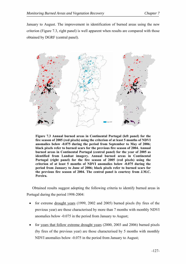
Monitoring Burned Areas and Vegetation Recovery Chapter 7
-127-
January to August. The improvement in identification of burned areas using the new
criterion (Figure 7.3, right panel) is well apparent when results are compared with those
obtained by DGRF (central panel).
Figure 7.3 Annual burned areas in Continental Portugal (left panel) for the fire season of 2005 (red pixels) using the criterion of at least 5 months of NDVI anomalies below -0.075 during the period from September to May of 2006; black pixels refer to burned scars for the previous fire season of 2004. Annual burned areas in Continental Portugal (central panel) for the year of 2005 as identified from Landsat imagery. Annual burned areas in Continental Portugal (right panel) for the fire season of 2005 (red pixels) using the criterion of at least 5 months of NDVI anomalies below -0.075 during the period from January to June of 2006; black pixels refer to burned scars for the previous fire season of 2004. The central panel is courtesy from J.M.C. Pereira.
Obtained results suggest adopting the following criteria to identify burned areas in
Portugal during the period 1998-2004:
• for extreme drought years (1999, 2002 and 2005) burned pixels (by fires of the
previous year) are those characterised by more than 7 months with monthly NDVI
anomalies below -0.075 in the period from January to August;
• for years that follow extreme drought years (2000, 2003 and 2006) burned pixels
(by fires of the previous year) are those characterised by 5 months with monthly
NDVI anomalies below -0.075 in the period from January to August;
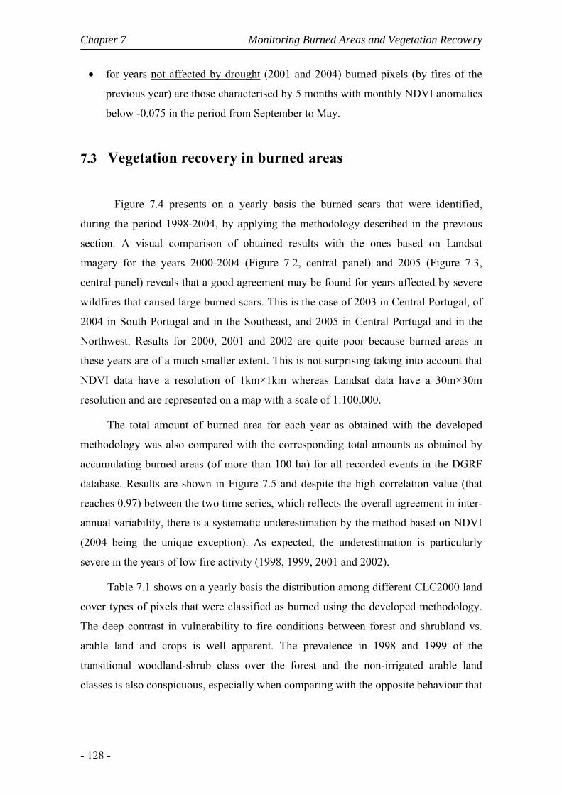
Chapter 7 Monitoring Burned Areas and Vegetation Recovery
- 128 -
• for years not affected by drought (2001 and 2004) burned pixels (by fires of the
previous year) are those characterised by 5 months with monthly NDVI anomalies
below -0.075 in the period from September to May.
7.3 Vegetation recovery in burned areas
Figure 7.4 presents on a yearly basis the burned scars that were identified,
during the period 1998-2004, by applying the methodology described in the previous
section. A visual comparison of obtained results with the ones based on Landsat
imagery for the years 2000-2004 (Figure 7.2, central panel) and 2005 (Figure 7.3,
central panel) reveals that a good agreement may be found for years affected by severe
wildfires that caused large burned scars. This is the case of 2003 in Central Portugal, of
2004 in South Portugal and in the Southeast, and 2005 in Central Portugal and in the
Northwest. Results for 2000, 2001 and 2002 are quite poor because burned areas in
these years are of a much smaller extent. This is not surprising taking into account that
NDVI data have a resolution of 1km×1km whereas Landsat data have a 30m×30m
resolution and are represented on a map with a scale of 1:100,000.
The total amount of burned area for each year as obtained with the developed
methodology was also compared with the corresponding total amounts as obtained by
accumulating burned areas (of more than 100 ha) for all recorded events in the DGRF
database. Results are shown in Figure 7.5 and despite the high correlation value (that
reaches 0.97) between the two time series, which reflects the overall agreement in inter-
annual variability, there is a systematic underestimation by the method based on NDVI
(2004 being the unique exception). As expected, the underestimation is particularly
severe in the years of low fire activity (1998, 1999, 2001 and 2002).
Table 7.1 shows on a yearly basis the distribution among different CLC2000 land
cover types of pixels that were classified as burned using the developed methodology.
The deep contrast in vulnerability to fire conditions between forest and shrubland vs.
arable land and crops is well apparent. The prevalence in 1998 and 1999 of the
transitional woodland-shrub class over the forest and the non-irrigated arable land
classes is also conspicuous, especially when comparing with the opposite behaviour that
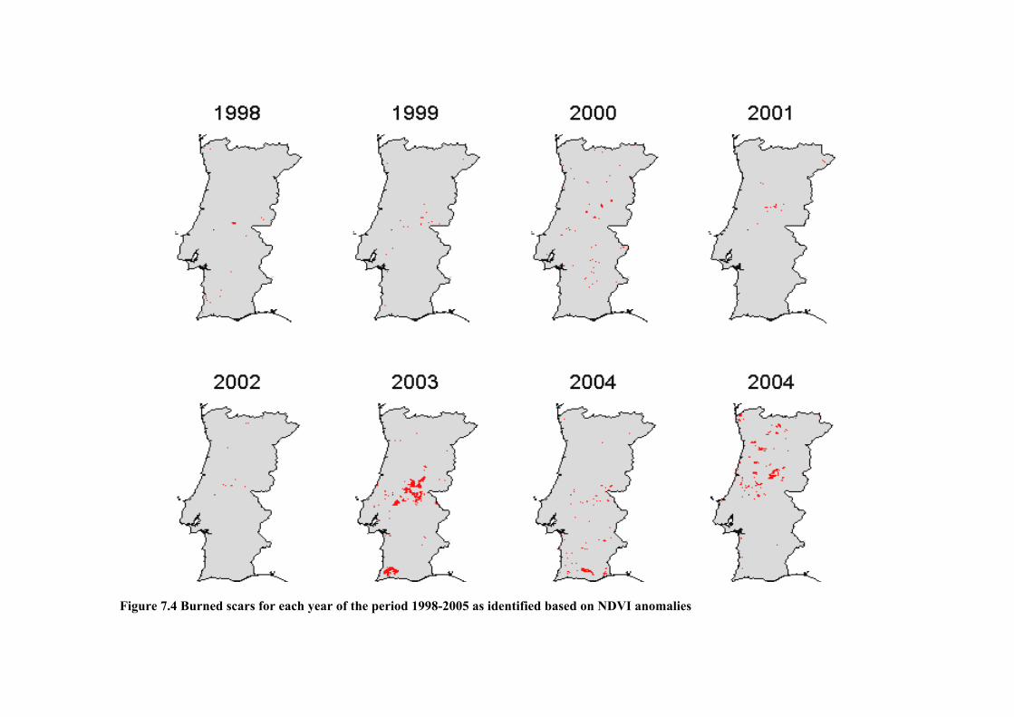
Figure 7.4 Burned scars for each year of the period 1998-2005 as identified based on NDVI anomalies
Chapter 7 Monitoring Burned Areas and Vegetation Recovery
-130-
Figure 7.5 Time series of annual burned areas in Continental Portugal for the period 1998-2005 as obtained from the developed methodology (solid line) and based on DGRF information (dotted curve).
Table 7.1 Percentage of burned pixels for pixels classified as non irrigated Arable Land, Forest, Transitional woodland-shrub and Shrubland (using Corine Land Cover Map 2000, CLC2000) for the fire seasons from the years 1998 to 2005.
Years Non
irrigated
arable land
Annual crops/
permanent
crops
Forest
Transitional
woodland-
-shrub
Shrubland Others
1998 11 1 21 38 4 19
1999 2 1 22 58 3 14
2000 16 4 23 18 9 30
2001 2 1 44 17 29 7
2002 0 0 76 16 3 5
2003 1 1 69 14 7 8
2004 4 1 55 8 9 23
2005 1 2 51 28 9 9
Monitoring Burned Areas and Vegetation Recovery Chapter 7
-131-
may be observed from 2000 onwards. However, this may be explained by the fact that
burned areas in 1998 and 1999 (i.e. in years immediately prior to 2000) were naturally
classified as transitional woodland-shrub according to CLC2000, meaning that
vegetation was still in the process of recovering from fire events. In the same context,
the sudden increase in 2005 of the percentage of burned pixels associated to transitional
woodland-shrub is also worth being noted. Such increase is due to the recurrence in
2005 of fires in regions that had burned prior to 2000.
Figure 7.6 shows, for selected pixels in a set of eight large fire scars, the
respective time series of NDVI, each one corresponding to an event that has occurred in
a given year of the considered 8-year period (1998-2005). The behaviour of the annual
cycles of NDVI, that display always a sharp decrease in the year of the fire event and a
steady increase in the following years, is a strong indication about the adequacy of the
adopted methodology. Results obtained further suggest using the procedure to assess
vegetation recovery after a large scale fire event.
An example of how vegetation recover assessment may be performed based on
the developed methodology is given in Figure 7.7. The figure presents the time series of
NDVI averaged over three large scars, two of them located in Central Portugal and
respecting to events in 2001 and 2003, and the third one located in Algarve and
respecting to an event in 2003. Differences in vegetation recovery are well apparent
between the two years and the two locations. In the case of the fire scars located in
Central Portugal it may be observed that the recovery is much faster in 2001 than in
2003, a feature that is explained by the fact that 2003 was followed by an extreme
drought event that started in 2004 and reached a peak in 2005. In the case of the event
of Algarve, the recovery is much slower than in the case of the event of the same year
that took place in Central Portugal. Again this may be partly explained by the fact that
drought conditions of 2004/2005 were particularly severe in the southern part of
Portugal (see Chapter 6).
Final remarks
We present a methodology aiming to identify large fire scars using monthly
values of NDVI at the 1km×1km spatial scale. The procedure is based on the analysis of

Chapter 7 Monitoring Burned Areas and Vegetation Recovery
-132-
Figure 7.6 Time series of NDVI for selected pixels in a set of eight large fire scars, each one corresponding to an event that has occurred in a given year of the 1998-2005. The location of the selected fire scars is given in the upper panel.
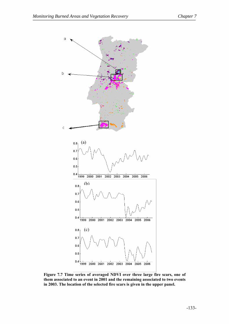
Monitoring Burned Areas and Vegetation Recovery Chapter 7
-133-
Figure 7.7 Time series of averaged NDVI over three large fire scars, one of them associated to an event in 2001 and the remaining associated to two events in 2003. The location of the selected fire scars is given in the upper panel.
(a)
(b)
(c)
Chapter 7 Monitoring Burned Areas and Vegetation Recovery
-134-
strongly negative anomalies of NDVI that persist during the vegetative cycle of the year
that follows the fire event.
Obtained results respecting to burned scars from fire events that have occurred in
the period 1998-2005 reveal that the developed methodology leads to an adequate
identification of burned areas for years affected by severe wildfires that caused large
burned scars. When comparing yearly amounts of burned area by the proposed method
with the corresponding ones from the official DGRF database, a systematic
underestimation is found, in particular in the case of years of low fire activity. However
the methodology based on NDVI anomalies allows monitoring the vegetation recovery
in areas affected by large fires.
A case study was performed involving two large burned areas in Central Portugal
associated to fire events that took place in 2001 and 2003 and a third one in Algarve
associated to a wildfire in 2003. Differences in vegetation recovery are well apparent
between the two years and the two locations, which were found to be mainly associated
to the meteorological conditions of the following year. In particular it was found that
vegetation recovery was slower for the two 2003 burned areas because of the prolonged
following drought of 2004/2005, especially in the case of Algarve where the effects of
drought were more severe.
8 CONCLUSIONS
Vegetation plays a crucial role in the global carbon balance because of the large
amounts of carbon stored in green vegetation. Over the last two decades, continuous
monitoring of vegetation from space has prompted new studies aiming to relate
observed major global changes in vegetation (e.g. trends, variability and extremes) with
changes in surface climatic variables, such as temperature and precipitation. Despite the
global nature of the problem, studies at the regional and local scales are especially
relevant in these contexts due to the socio-economical impacts in land management.
The primary motivation of our work was to contribute to a better understanding
of the impact of climate variability on vegetation status and dynamics at the European
scale, but in particular at the scale of Continental Portugal. We began by assessing the
relationship between vegetation greenness and the NAO index. The study covered the
21-year period of available homogeneous datasets from 1982 to 2002, and was based on
monthly composites of NDVI and Brightness Temperature from GIMMS dataset as well
as on monthly precipitation from GPCC. A systematic analysis was initially performed
of point correlation fields over the 21-year period between the winter NAO index and
the spring and summer NDVI. An assessment was then performed on the vegetation
response to precipitation and temperature conditions in winter, over two contrasting
regions, namely the Iberian Peninsula and Northeastern Europe. The impact of NAO on
vegetation dynamics over the two considered regions was finally evaluated by studying
the corresponding annual cycles of NDVI and then comparing their behaviour for years
associated with opposite NAO phases.
There is strong evidence that positive (negative) values of winter NAO induce
low (high) vegetation activity, over the Iberian Peninsula, in the following spring and
summer seasons. This feature is mainly associated with the impact of NAO on winter
precipitation, together with the strong dependence of spring and summer vegetation on
water availability during the previous winter. In Iberia, the NAO impact is larger on
non-forested vegetation, which responds quickly to spatio-temporal variations in
precipitation and soil moisture. During summer, forests and other dense vegetation areas

Chapter 8 Conclusions
-136-
display the highest sensitivity to NAO dynamics, as well as a slower response to
precipitation, the NAO impacts being delayed until late in the year. Obtained results, in
particular those related to the relationships found between winter NAO and NDVI for
spring and summer represent an added value since they allow formulating simple
outlooks of vegetation greenness that may provide useful information for a wide range
of application, such as crop forecasting and long-lead wild fire assessment.
In this context, we have further investigated how variations in vegetation
greenness over Continental Portugal might be related with NDVI as derived from the
GIMMS database. We have focused on wheat yield for the period 1982-1999 and
strongly negative correlations were found between wheat yield and spring NDVI over
the wheat production area located in Southern Portugal (Alentejo). The impact of
meteorological factors on wheat yield over this region was also assessed by computing
monthly correlations of detrended anomalies of yield with net short-wave radiation,
temperature and precipitation as well as with NAO. Results obtained indicate that cold
temperatures during winter and early spring, precipitation in February and March and
solar radiation in March have a positive impact during the growing stage, whereas a
larger NAO index in June is beneficial for the maturation stage. Therefore, a simple
multi-linear regression model was built up using, as predictors, the values of spring
NDVI and NAO in June. Simple and cross-validation have confirmed that the
performance of such a straightforward model can be quite satisfactory, with a general
agreement between observed and modelled wheat yield.
NDVI fields as derived from the VEGETATION instrument were also used to
monitor drought episodes. The severity of a given drought episode was assessed by
evaluating the cumulative impact over time of drought conditions on vegetation. Special
attention was given to the drought episode of 2005, as well as to those that took place in
1999 and 2002. The impact of soil moisture on vegetation dynamics was also evaluated
by studying the annual cycle of SWI vs. NDVI and by analysing monthly anomalies of
SWI. While in the case of the drought episode of 1999 the scarcity of water in the soil
persisted until spring, in the recent episode of 2005 the deficit in greenness was already
apparent at the end of summer. The impact of dry periods on vegetation was clearly
observed in both arable land and forest, and it was found that arable land presented a
higher sensitivity.
Chapter 8 Conclusions
-137-
Persistence of negative anomalies of NDVI was also used to develop a procedure
aiming to identify burned scars and assess vegetation recovery over areas stricken by
wildfires. Obtained results indicated that the developed methodology is adequate to
identify large burned areas. The vulnerability of land cover to wildfire was also assessed
and a strong contrast was found between forest and shrubland vs. arable land and crops.
The high percentage of burned pixels that were found to belong to the transitional
woodland-shrub class may provide and indication of the repeated occurrence of
wildfires, which may accelerate the switch of forest into shrub-woodland vegetation,
with important consequences in a country where transitional woodland-shrub vegetation
is the third more frequent land cover. The developed methodology based on persistent
NDVI anomalies also allowed monitoring vegetation recovery in areas affected by large
fires. Evidence was found that vegetation recovery may strongly depend on the
meteorological conditions of the following year. In fact, vegetation recovery was
especially slow in 2003 because of the following drought of 2004/2005, in particular in
the case of Algarve where the effects of drought were more severe.
The main conclusions from our study may be summarized as follows:
• the impact of climate variability on vegetation dynamics, as response to
precipitation and temperature conditions in winter, is well apparent in Iberian
Peninsula and Northeastern Europe;
• there is strong evidence that positive (negative) values of winter NAO induce low
(high) vegetation activity, over the Iberian Peninsula, in the following spring and
summer seasons;
• the lagged relation between winter NAO and spring and summer NDVI may be
used to build-up models of crop forecasting and long-lead fire assessment;
• the impact of climate variability on wheat yield in Portugal may be used to
build-up models of wheat yield;
• drought conditions in Portugal may be adequately monitored using remote sensed
information and drought severity may be assessed based on the persistence of
NDVI anomalies;
• persistent anomalies of NDVI may be also used to identify burned areas and to
assess vegetation recovery after large wildfires.


REFERENCES
Alley, W.M., 1984: The Palmer Drought Severity Index: Limitations and assumptions.
Journal of Climate and Applied Meteorology, 23, 1100–1109.
Atkinson, M.D., Kettlewell, P.S., Hollins, P.D, Stephenson, D.B. and Hardwick, N.V.,
2005: Summer climate mediates UK wheat quality response to winter North Atlantic
Oscillation. Agricultural and Forest Meteorology, 130, 27–37.
Barnston, A.G., Livezey, R.E., 1987: Classification, Seasonality and Persistence of
Low-Frequency Atmospheric Circulation Patterns. Monthly Weather Review, 115,
1083-1126.
Bayarjargal, Y., Karnieli, A., Bayasgalan, M., Khudulmur, S., Gandush, C. and Tucker,
C.J., 2006: A comparative study of NOAA-AVHRR derived drought indices using
change vector analysis. Remote Sensing of Environment, 105(1), 9-22.
Benson, B.J., and MacKenzie, M.D., 1995: Effects of sensor spatial resolution on
landscape structure parameters. Landscape Ecology, 10, 113-120.
Blenckner, T, Hillebrand, H., 2002: North Atlantic Oscillation signatures in ecosystems
- a meta-analysis. Global Change Biology, 8, 203-212.
Bogaert, J, Zhou, L, Tucker, C.J., Myneni, R.B., Ceulemans, R., 2002: Evidence for a
persistent and extensive greening trend in Eurasia inferred from satellite vegetation
index data. Journal of Geophysical Research, 107(D11), DOI:
10.1029/2001JD00107.
Boken, V.K. and Shaykewich, C.F., 2002: Improving an operational wheat yield model
using phonological phase-based Normalized Difference Vegetation Index.
International Journal of Remote Sensing, 23(20), 4155–4168.
Bonifacio, R., Dugdale, G. and Milford, J.R., 1993: Sahelian rangeland production in
relation to rainfall estimates from Meteosat. International Journal of Remote
Sensing, 14, 2695–2711.
References
-140-
Briffa, K.R., Jones, P.D. and Hulme, M., 1994: Summer moisture variability across
Europe, 1892–1991: an analysis based on the Palmer drought severity index.
International Journal of Climatology, 14, 475–506.
Brooks, M.L. and Pyke, D.A., 2001: Invasive plants and fire in the deserts of North
America. In K. Galley and T. Wilson (Eds.), Fire Conference 2000: The First
National Congress on Fire, Ecology, Prevention and Management. Invasive Species
Workshop: The Role of Fire in the Control and Spread of Invasive Species (pp. 1-
14). Tallahassee: Tall Timbers Research Station.
Buermann, W., Anderson, B., Tucker, C.J., Dickinson, R.E., Lucht, W., Potter, C.S. and
Myneni, R.B., 2003: Interannual covariability in Northern Hemisphere air
temperatures and greenness associated with El Niño-southern oscillation and the
Arctic Oscillation. Journal of Geophysical Research, 108, 4396,
DOI:10.1029/2002JD002.
Bussay, A., Szinell, C., Szentimery, T., 1999: Investigation and Measurements of
Droughts in Hungary. Hungarian Meteorological Service: Budapest.
Castro-Díez, Y., Pozo-Vázquez, D., Rodrigo, F.S. and Esteban-Parra, M.J., 2002: NAO
and winter temperature variability in southern Europe. Geophysical Research Letters,
29, DOI:10.1029/ 2001GL014042.
Cerda, A., 1998a: Changes in overland flow and infiltration after a rangeland fire in a
Mediterranean scrubland. Hydrological Processes, 12, 1031–1042.
Cerda, A., 1998b: Postfire dynamics of erosional processes under Mediterranean
climatic conditions. Zeitschrift für Geomorphologie, 42, 373–398.
Cerda, A. and Doerr, S.H., 2005: The influence of vegetation recovery on soil
hydrology and erodibility following fire: an eleven year investigation. International
Journal of Wildland Fire, 14(4), 423–437.
Chatterjee, S., Hadi, A.S., 1986: Influential observations, high leverage points, and
outliers in linear regression. Statistical Science, 1(3), 379-416.
Chen, J.M. and Cihlar, J., 1996: Retrieving leaf area index for boreal conifer forests
using Landsat TM images. Remote Sensing of Environment, 55, 153-162.
Ciais, Ph., Reichstein, M., Viovy, N., Granier, A., Ogée, J., Allard, V., Aubinet, M.,
Buchmann, N., Bernhofer, Chr., Carrara, A., Chevallier, F., De Noblet, N., Friend,
References
-141-
A.D., Friedlingstein, P., Grünwald, T., Heinesch, B., Keronen, P., Knohl, A.,
Krinner, G., Loustau, D., Manca, G., Matteucci, G., Miglietta, F., Ourcival, J.M.,
Papale, D., Pilegaard, K., Rambal, S., Seufert, G., Soussana, J.F., Sanz, M.J.,
Schulze, E.D., Vesala, T. and Valentini, R., 2005: Europe-wide reduction in primary
productivity caused by the heat and drought in 2003. Nature, 437, 529–533.
Colwell, R.N., 1997: History and Place of Photographic Interpretation. In M.D.
Bethesda (Ed.), Manual of Photographic Interpretation (pp. 33–48). American
Society for Photogrammetry & Remote Sensing.
Cook, B.I., Mann, M.E., D’Odorico, P. and Smith, T.M., 2004: Statistical simulation of
the influence of the NAO on European winter surface temperatures: Applications to
phenological modeling. Journal of Geophysical Research, 109(D16106),
DOI:10.1029/2003JD004305.
Cracknell, A.P., 1998: Synergy in remote sensing – what’s in a pixel?. International
Journal of Remote Sensing, 19(11), 2025-2047.
Crippen, R.E., 1987: The Regression Intersection Method of Adjusting Image Data for
Band Ratioing. International Journal of Remote Sensing, 8, 137-155.
Davidson, E.A. and Janssens, I.A., 2006: Temperature sensitivity of soil carbon
decomposition and feedbacks to climate change. Nature, 440, 165–173.
DeBano, L.F., Neary, D.G. and Ffolliott, P.F., 1998: Fire's Effects on Ecosystems. John
Wiley and Sons, Inc., New York, 333 pp.
DeMelo, R.W., Fontana, D.C., Berlato, M.A. and Ducati, J.R., 2008: An
agrometeorological-spectral model to estimate soybean yield, applied to southern
Brazil. International Journal of Remote Sensing, 29(14), 4013- 4028.
Denman, K.L., Brasseur, G., Chidthaisong, A., Ciais, P., Cox, P.M., Dickinson, R.E.,
Hauglustaine, D., Heinze, C., Holland, E., Jacob, D., Lohmann, U., Ramachandran,
S, da Silva Dias, P.L., Wofsy, S.C. and Zhang, X., 2007: Couplings Between
Changes in the Climate System and Biogeochemistry. In S. Solomon, D. Qin, M.
Manning, Z. Chen, M. Marquis, K.B. Averyt, M. Tignor and H.L. Miller (Eds.),
Climate Change 2007: The Physical Science Basis. Contribution of Working Group I
to the Fourth Assessment Report of the Intergovernmental Panel on Climate Change

References
-142-
(pp. 499-587). Cambridge University Press, Cambridge, United Kingdom and New
York, NY, USA. Available at: http://ipcc-wg1.ucar.edu/wg1/wg1-report.html.
Díaz-Delgado, R., Salvador, R. and Pons, X., 1998: Monitoring of plant community
regeneration after fire by remote sensing. In L. Traboud (Ed.), Fire management and
landscape ecology (pp. 315-324). International Association of Wildland Fire,
Fairfield, WA.
Díaz-Delgado, R., Lloret, F., Pons, X. and Terradas, J., 2002: Satellite evidence of
decreasing resilience in Mediterranean plant communities after recurrent wildfires.
Ecology, 83(8), 2293–2303.
Diouf, A. and Lambin, E.F., 2001: Monitoring land-cover changes in semi-arid regions:
Remote sensing data and field observations in the Ferlo, Senegal. Journal of Arid
Environments, 48, 129 148.
D’Odorico, P., Yoo, J.C. and Jaeger, S., 2002: Changing seasons: an effect of the North
Atlantic Oscillation? Journal of Climate, 15, 435-445.
Drury, S., 1987: Display and enhancement of gridded aeromagnetic data of the Solway
Basin. International Journal of Remote Sensing, 8(10), 1433-1444.
Dube, O.P., 2007: Fire Weather and Land Degradation. In Springer Berlin Heidelberg
(Ed.), Climate and Land Degradation (pp. 223-251). ISBN 978-3-540-72437-7. DOI
10.1007/978-3-540-72438-4
Eagleson, P., 2002: Ecohydrology. Darwinian expression of vegetation form and
function. Cambridge University Press, Cambridge, 2002.
EEA, 2001: Sustainable water use in Europe, Part 3: extreme hydrological events:
floods and droughts. Environmental Issue Report No. 21. European Environment
Agency.
EPSG, 2002: Coordinate Conversions and Transformations including Formulas,
Guidance Note Number 7, Petrochemical Open Software Corporation (POSC).
Available at: http://www.ihsenergy.com/epsg/guid7.pdf
Estrela, M.J., Penarrocha, D. and Mill´ na, M,. 2000: Multi-annual drought episodes in
the Mediterranean (Valencia region) from 1950–1996. A spatio-temporal analysis.
International Journal of Climatology, 20, 1599–1618.

References
-143-
Fang, H., Liang, S., Hoogenboom, G., Teasdale, J. and Cavigelli, M., 2008: Corn-yield
estimation through assimilation of remotely sensed data into the CSM-CERES-Maize
model. International Journal of Remote Sensing, 29(10), 3011-3032.
Feio, M. and Henriques, V., 1986: As secas de 1980–81 e de 1982–83 e as principais
secas anteriores – intensidade e distribuição regional. Memórias do Centro de
Estudos Geográficos, 10, 7–113.
Feio, M., 1991: Clima e Agricultura. Ministério da Agricultura, Pescas e Alimentação.
Gámiz-Fortis, S.D., Pozo-Vázquez, D., Rodrigo, F.S., Esteban-Parra, M.J. and Castro-
Díez, Y., 2002: Spectral characteristics and predictability of the NAO assessed
through Singular Analysis. Journal of Geophysical Research, 107, 4685.
DOI:10.1029/2001JD001436.
Garcia-Herrera, R., Paredes, D., Trigo, R.M., Trigo, I.F., Hernández, H., Barriopedro D.
and Mendes, M.T., 2007: The outstanding 2004-2005 drought in the Iberian
Peninsula: the associated atmospheric circulation. Journal of Hydrometeorology, (in
press).
Gibb, O, Penman, H.L., Pereier, H.C. and Ratcliffe, R.A.S., 1978: Scientific Aspects of
the 1975–76 Drought in England and Wales. The Royal Society: London.
Gilbert, E.N., 1974: Distortion in maps. SIAM Review, 16(1), 47-62.
Gimeno, L., Ribera, P., Iglesias, R., Torre, L., Garcia, R. and Hernández, E, 2002:
Identification of empirical relationships between indices of ENSO and NAO and
agricultural yields in Spain. Climate Research, 21, 165–172.
Gobron, N., Pinty, B. and Verstraete, M.M., 1997: Theoretical Limits to the Estimation
of the Leaf Area Index on the Basis of Visible and Near-Infrared Remote Sensing
Data. IEEE Transactions on Geoscience and Remote Sensing, 35, 1438-1445.
Gobron, N., Pinty, B., Verstraete, M.M. and Widlowski, J.-L., 2000: Advanced
Vegetation Indices Optimized for Up-Coming Sensors: Design, Performance and
Applications. IEEE Transactions on Geoscience and Remote Sensing, 38, 2489-
2505.
Gobron, N., Mélin, F., Pinty, B., Verstraete, M.M., Widlowski, J.-L., and Bucini, G.,
2001: A Global Vegetation Index for SeaWiFS: Design and Applications. In M.
References
-144-
Beniston and M. M. Verstraete (Eds.), Remote Sensing and Climate Modelling:
Synergies and Limitations (pp. 5-21). Kluwer Academic Publishers, Dordrecht.
Gobron, N., Pinty, B., Mélin, F., Taberner M. and Verstraete, M.M., 2002: Sea Wide
Field-of-View Sensor (SeaWiFS) - An Optimized FAPAR Algorithm - Theoretical
Basis Document. EUR Report No. 20148 EN (pp. 20), Institute for Environment and
Sustainability.
Gobron, N., Pinty, B., Mélin, F., Taberner M., Verstraete, M.M., Belward, A.,
Lavergne, T. and Widlowski, J.-L., 2005: The state of vegetation in Europe
following the 2003 drought. International Journal of Remote Sensing Letters, 26,
2013–2020.
Godinho, S.F., Mendes, J.C. and Reis, R.M., 1992: A Situação de Seca em Portugal
iniciada no Inverno de 1991/92. Ambiente, 6, 18–25.
Gouveia, C. and Trigo, R.M., 2008: Infuence of Climate Variability on Wheat
Production in Portugal. In A. Soares, M.J. Pereira and R. Dimitrakopoulos (Eds.),
geoENV VI -Geostatistics for Environmental Applications (pp.335-345). Springer.
Govaerts, Y.M., Verstraete, M.M., Pinty, B. and Gobron, N., 1999: Designing optimal
spectral indices: A feasibility and proof of concept study. International Journal of
Remote Sensing, 20, 1853–1873.
Groisman, P.Y., Karl, T.R. and Knight, R.W., 1994: Observed impact of snow cover on
the heat balance and the rise of continental spring temperatures. Science, 263, 198-
200.
Hagolle, O., Lobo, A., Maisongrande, P., Duchemin, B., and De Pereira, A., 2005:
Quality assessment and improvement of SPOT/VEGETATION level temporally
composited products of remotely sensed imagery by combination of VEGETATION
1 & 2 images. Remote Sensing of Environment, 94(2), 172–186.
Hansen, J., Ruedy, R., Glascoe, J., Sato, M., 1999: GISS analysis of surface temperature
change. Journal of Geophysical Research, 104, 30997-31022.
Heimann, M. and Reichstein, M., 2008: Terrestrial ecosystem carbon dynamics and
climate feedbacks. Nature, 451, 289-292.

References
-145-
Henry, M.C. and Hope, A.S., 1998: Monitoring post-burn recovery of chaparral
vegetation in southern California using multitemporal satellite data. International
Journal of Remote Sensing, 19(16), 3097–3107.
Holben, B.N., Tucker C.J. and Fan, C-J., 1980: Spectral Assessment of Soybean Leaf
Area and Leaf Biomass. Photogrammetric Engineering and Remote Sensing, 46,
651-656.
Holben, B.N., 1986: Characteristics of maximum-value composite images from
temporal AVHRR data. International Journal of Remote Sensing, 7, 1417–1434.
Holmgren, M. and Scheffer, M., 2001: El Niño as a window of opportunity for the
restoration of degraded arid ecosystems. Ecosystems, 4, 151-159.
Holmgren, M., Stapp, P., Dickman, C.R., Gracia, C., Grahams, S., Gutierrez, J.R., Hice,
C., Jaksic, F., Kelt, D.A., Letnic, M., Lima, M., Lopez, B.C., Meserve, P.L.,
Milstead, W.B., Polis, G.A., Previtali, M.A., Michael, R., Sabate, S., and Squeo,
F.A., 2006: Extreme climatic events shape arid and semiarid ecosystems. Frontiers
in Ecology and the Environment, 4, 87–95.
Hoogenboom, G, 2000: Contribution of agrometeorology to the simulation of crop
production and its applications. Agricultural and Forest Meteorology, 103, 137-158.
Huang, N.E., Shen, Z., Long, S.R., Wu, M.C., Shih, H.H., Zheng, Q., Yen, N.-C., Tung,
C.C. and Liu, H.H., 1998: The empirical mode decomposition and the Hilbert
spectrum for nonlinear and non-stationary time series analysis. Proceedings from the
Royal Society of London, 545, 903-995.
Huang, N.E., Shen, Z. and Long, S.R., 1999: A new view of nonlinear water waves: the
Hilbert spectrum. Annual Review of Fluid Mechanics, 31, 417-457.
Huete, A.R. and Tucker, C.J., 1991: Investigation of soil influences on AVHRR red and
near-infrared vegetation index imagery. International Journal of Remote Sensing, 12,
1223 1242.
Hurrell, J.W., 1995: Decadal trends in the north Atlantic oscillation: regional
temperatures and precipitation. Science, 269, 676–679.
Iglesias, A., Quiroga, S., 2007: Measuring the risk of climate variability to cereal
production at five sites in Spain. Climate Research, 34, 47–57.

References
-146-
Iglesias, E., Garrido, A. and Gomez-Ramos, A., 2003: Evaluation of drought
management in irrigated areas. Agricultural Economics, 29, 211–229.
Illera, P., Fernandez, A. and Delgado, J.A., 1996: Temporal evolution of the NDVI as
an indicator of forest fire danger. International Journal of Remote Sensing, 17(6):
1093–1105.
Inbar, M., Wittenberg, L. and Tamir, M., 1997: Soil erosion and forestry management
after wildfire in a Mediterranean woodland, Mt. Carmel, Israel. International Journal
of Wildland Fire, 7(1997), 285–294.
Inbar, M., Tamir, M. and Wittenberg, L., 1998: Runoff and erosion processes after a
forest fire in Mount Carmel, a Mediterranean area. Geomorphology, 24(1) (1998),
17–33.
Jakubauskas, M., Lulla, K.P., and Mausel, P.W., 1990: Assessment of vegetation
change in a fire-altered forest landscape. Photogrammetric Engineering & Remote
Sensing, 56, 371-377.
Jensen, J.R., 2005: Introductory Digital Image Processing: A Remote Sensing
Perspective. 3rd Edition. Prentice Hall Inc., 526pp.
Jensen, J.R., 2007: Remote Sensing of the Environment: An Earth Resource Perspective.
2nd Edition. Prentice-Hall, Inc., Saddle River, N.J., 544 pp.
Ji, L. and Peters, A.J., 2003: Assessing vegetation response to drought in the northern
Great Plains using vegetation and drought indices. Remote Sensing of Environment,
87, 85-98.
Jones, P.D., Johnson, T. and Wheeler, D., 1997: Extension to the North Atlantic
Oscillation using instrumental pressure observations from Gibraltar and south-west
Iceland. International Journal of Climatology, 17, 1433–1450.
Justice, C., Dorn, B., Hansen, M., Tucker, J., Anyamba, A., Sullivan, M. and Reshef, I.,
2005: Global Agricultural Monitoring: Science Information to Inform Decision
Making. U.S. Climate Change Science Program (CCSP) Workshop on Climate
Science in Support of Decision Making, Arlington, Virgina, 14-16 November 2005.
Karl, T., 1986: The sensitivity of the Palmer drought severity index and Palmer's Z-
index to their calibration coefficients including potencial evapotranspiration. Journal
of Climate and Applied Meteorology, 25, 77-86.
References
-147-
Karnieli, A., Shachak, M., Tsoar, H., Zaady, E., Kaufman, Y., Danin, A. and Porter, W.,
1996: The effect of Microphytes on the spectral reflectance of vegetation in semi-
arid regions. Remote Sensing of Environment, 57, 88–96
Kaufmann, R.K., Zhou, L., Knyazikhin, Y., Shabanov, N., Myneni, R.B. and Tucker,
C.J., 2000: Effect of orbital drift and sensor changes on the time series of AVHRR
vegetation index data. IEEE Transactions Geoscience and Remote Sensing, 38,
2584–2597.
Kaufmann, R.K., Zhou, L., Tucker, C.J., Slayback, D., Shabanov, N.V. and Myneni,
R.B., 2002: Reply to Comment on ‘Variations in northern vegetation activity inferred
from satellite data of vegetation index during 1981-1999 by J.R. Ahlbeck. Journal of
Geophysical Research, 107(D11), DOI:10.1029/2001JD001516.
Keeling, C.D., Chin, J.F.S. and Whorf, T.P., 1996: Increased activity of northern
vegetation inferred from atmospheric CO2 measurements. Nature, 382, 146-149.
Knapp, A.K., Fay, P.A., Blair, J.M., Collins, S.L., Smith, M.D., Carlisle, J.D., Harper,
C.W., Danner, B.T., Lett, M.S. and McCarron, J.K., 2002: Rainfall variability,
carbon cycling, and plant species diversity in a mesic grassland. Science, 298, 2202–
2205.
Kogan, F.N., 1995: Application of vegetation index and brightness temperature for
drought detection. Advances in Space Research, 11, 91-100.
Kogan, F.N., 1997. Global drought watch from space. Bulletin of the American
Meteorological Society, 78, 621-636.
Kogan, F.N., 2000. Contribution of remote sensing to drought early warning. In D.A.
Wilhite, M.V.K. Sivakumar and D.A. Wood (Eds.), Early warning systems for
drought preparedness and drought management: Proceedings of an Expert Group
Meeting, 5–7 September, Lisbon, Portugal (pp. 86-100). Geneva, Switzerland:
WMO.
Kogan, F.N., Usa, D.C., Stark, R., Gitelson, A., Jargalsaikhan, L. and Dugarjav, C.,
2004: Derivation of pasture biomass in Mongolia from AVHRR-based vegetation
health indices. International Journal of Remote Sensing, 25, 2889 2896.
Kutiel, P., 1994: Fire and ecosystem heterogeneity: a Mediterranean case study. Earth
Surface Processes and Landforms, 19, 187–194.

References
-148-
Lana, X., Serra, C. and Burgueño, A., 2001: Patterns of monthly rainfall shortage and
excess in terms of the standardized precipitation index. International Journal of
Climatology, 21, 1669–1691.
Le Page, Y., Pereira, J.M.C., Trigo, R.M., DaCamara, C.C., Oom, D., and Mota, B.,
2008: Global fire activity patterns (1996-2006) and climatic influence: an analysis
using the World Fire Atlas. Atmospheric Chemistry and Physics, 8, 1911-1924.
Li, Y., Demetriades-Shah, T.H., Kanemasu, E.T., Shultis, J.K. and Kirkham, M.B.,
1993: Use of Second Derivatives of Canopy Reflectance for Monitoring Prairie
Vegetation Over Different Soil Backgrounds. Remote Sensing of Environment, 44,
81-87.
Lloyd-Hughes, B. and Saunders, M.A., 2002: A drought climatology for Europe.
International Journal of Climatology, 22(13), 1571-1592.
Los, S.O., 1998: Estimation of the ratio of sensor degradation between NOAA-AVHRR
channels 1 and 2 from monthly NDVI composites. IEEE Transactions on Geoscience
and Remote Sensing, 36, 206-213.
Los, S.O., 1998: Linkages between global vegetation and climate: an analysis based on
NOAA-Advanced Very High Resolution Radiometer Data. Doctoral Thesis, Vrije
Universiteit, Amsterdam.
Lotsch, A., Tian, Y., Friedl, M.A. and Myneni, R.B., 2003: Land cover mapping in
support of LAI/FPAR retrievals from EOS-MODIS and MISR: Classification
methods and sensitivities to errors. International Journal of Remote Sensing, 24,
1997-2016.
Lucht, W.I., Colin Prentice, W.I., Myneni, R.B., Sitch, S., Friedlingstein, P., Cramer,
W., Bousquet, P., Buermann, W., and Smith, B., 2002: Climatic Control of the High-
Latitude Vegetation Greening Trend and Pinatubo Effect. Science, 296, 1687–1688.
MADRP, 2005: Relatório de balanço da seca. Ministério da Agricultura do
Desenvolvimento Rural e Pescas, Lisboa.
Malingreau, J.P., Stephens, G. and Fellows, L., 1985: Remote sensing of forest fires:
Kalimantan and North Borneo in 1982–83. Ambio, 14, 314–321.
Malingreau, J.P., 1986: Global vegetation dynamics: Satellite observations over Asia.
International Journal of Remote Sensing, 9, 1121 1146.

References
-149-
Marsh, T.J., Lees, M.L., 1985: The 1984 Drought. Institute of Hydrology: Wallingford,
UK.
Maytelaube, P., Terres, J.-M. and Doblas-Reyes, F.J., 2004: Influence of climate
variability on European agriculture —analysis of winter wheat production. Climate
Research, 27, 135–144.
McVicar, T.R., and Jupp, D.L.B., 1998: The current and potential operational uses of
remote sensing to aid decisions on drought exceptional circumstances in Australia: A
review. Agricultural Systems, 57, 399-468.
McVicar, T.R. and Jupp, D.L.B., 1999: Estimating one-time-of-day meteorological data
from standard daily data as inputs to thermal remote sensing based energy balance
models. Agriculture and Forest Meteorology, 96, 219-238.
McVicar, T.R. and Jupp, D.L.B., 2002: Using covariates to spatially interpolate
moisture availability in the Murray-Darling Basin: A novel use of remotely sensed
data. Remote Sensing of Environment, 79, 199-212.
Menzel, A., 2003: Plant Phenological Anomalies in Germany and their Relation to Air
Temperature and NAO. Climatic Change, 57, 243-263.
Michelsen, A., Andersson, M., Jensen, M., Kjøller, A. and Gashew, M., 2004: Carbon
stocks, soil respiration and microbial biomass in fire-prone tropical grassland,
woodland and forest ecosystems. Soil Biology & Biochemistry, 36, 1707-1717.
Miranda, P.M.A., Valente, M.A., Tomé, A.R., Trigo, R., Coelho, M.F., Aguiar, A. and
Azevedo E.B., 2006: O Clima de Portugal nos séculos XX e XXI. In Santos, F.D.,
Forbes K. and Moita R. (Eds.), Climate Change in Portugal: Scenarios, Impacts and
Adaptation Measures - SIAM II Project (pp. 47-113). Gradiva, Lisbon.
Mitchell,T.D. and Jones, P.D., 2005: An improved method of constructing a database of
monthly climate observations and associated high-resolution grids. International
Journal of Climatology, 25, 693-712.
Moik, J.G., 1980: Digital Processing of Remotely Sensed Images. Washington D.C.,
NASA, U.S. Government Printing Office, 330 pp.
Morales, A., Olcina, J. and Rico, A.M., 2000: Diferentes percepciones de la sequía en
España: adaptación, catastrofismo e intentos de corrección (The different perceptions

References
-150-
about droughts in Spain: adaptations and correction systems, in Spanish).
Investigaciones Geográficas, 23, 5–46.
Myneni, R.B. and Williams, D.L., 1994: On the relationship between FPAR and NDVI.
Remote Sensing of Environment, 49, 200–211.
Myneni, R.B., Keeling, C.D., Tucker, C.J., Asrar, G. and Nemani, R.R., 1997. Increase
plant growth in the northern high latitudes from 1981-1991. Nature, 386, 698-702.
Neitsch, S.L., Arnold, J.G., Kiniry, J.R., Williams, J.R. and Kiniry, K.W., 2002: Soil
and Water Assessment Tool theoretical documentation. TWRI report TR-191, Texas
Water Resources Institute, College Station.
Nemani, R.R., Charles, D., Keeling, C.D., Hashimoto, H., Jolly, W.M., Piper, S.C.,
Tucker, C.J., Myneni, R.B. and Running, S.W., 2003: Climate-Driven Increases in
Global Terrestrial Net Primary Production from 1982 to 1999. Science, 300, 1560–
1563.
New, M., Hulme, M. and Jones, P.D., 1999: Representing twentieth century space-time
climate variability. Part 1: development of a 1961-90 mean monthly terrestrial
climatology. Journal of Climate, 12, 829-856.
New, M., Hulme, M. and Jones, P.D., 2000: Representing twentieth century space-time
climate variability. Part 2: development of 1901-96 monthly grids of terrestrial
surface climate. Journal of Climate, 13, 2217-2238.
Nicholson, S.E., Davenport, M.L., and Malo, A.R., 1990: A comparison of the
vegetation response to rainfall in the Sahel and east Africa, using normalized
difference vegetation index from NOAA-AVHRR. Climatic Change, 17, 209–241.
Nicholson, S.E., and Farrar, T.J., 1994. The influence of soil type on the relationships
between NDVI, rainfall, and soil moisture in semiarid Botswana: I. NDVI response
to rainfall. Remote Sensing of Environment, 50, 107 120.
Nicholson, S.E., Tucker, C.J., and Ba, M.B., 1998: Desertification, drought and surface
vegetation: An example from the West African Sahel. Bulletin of the American
Meteorological Society, 79, 815-829.
Osborn, T.J., Briffa, K.R., Tett, S.F.B., Jones, P.D., and Trigo, R.M., 1999: Evaluation
of the North Atlantic Oscillation as simulated by a climate model. Climate
Dynamics, 15, 685–702.

References
-151-
Palmer, W.C., 1965: Meteorological drought. Research Paper No. 45, U.S. Department
of Commerce Weather Bureau, Washington, D.C.
Paltridge, G.W. and Barber, J., 1988: Monitoring grassland dryness and fire potential in
Australia with NOAA–AVHRR data. Remote Sensing of Environment, 25, 381–394.
Paredes D., Trigo, R.M., Garcia-Herrera, R., Trigo, I.F., 2006: Understanding
precipitation changes in Iberia in early Spring: weather typing and storm-tracking
approaches. Journal of Hydrometeorology, 7, 101-113.
Pausas, G.J. and Vallejo, V.R., 1999: The role of fire in European Mediterranean
Ecosystems. In: E. Chuvieco (Ed.), Remote sensing of large wildfires in the
European Mediterranean basin (pp. 3–16). Springer–Verlag (1999).
Pereira, J.S., Pereira, J.M.C., Rego, F.C., Silva, J.M.N. and Silva, T.P., 2006: Incêndios
florestais em Portugal: caracterização, impactes e prevenção. ISA Press, Lisboa.
Pettorelli, N., Vik, J.O, Mysterud, A., Gaillard, J.-M. Tucker, C. J., Stenseth, N. C.,
2005: Using the satellite-derived NDVI to assess ecological responses to
environmental change. Trends in Ecology and Evolution, 20, 503-510.
Phillips, I.D. and McGregor, G.R., 1998: The utility of a drought index for assessing the
drought hazard in Devon and Cornwall, South West England. Meteorological
Applications, 5, 359–372.
Piao, S., Ciais, P., Friedlingstein, P., Peylin, P., Reichstein, M., Luyssaert, S., Margolis,
H., Fang, J., Barr, A., Chen, A,. Grelle, A., Hollinger, D.Y., Laurila, T., Lindroth, A.,
Richardson, A.D., and Vesala, T., 2008: Net carbon dioxide losses of northern
ecosystems in response to autumn warming. Nature, 451, 49-52.
Pielke, R.A., 2001: Influence of the spatial distribution of vegetation and soils on the
prediction of cumulus convective rainfall. Reviews of Geophysics, 39, 151–177.
Pinzon, J., Pierce, J.F. and Tucker, C.J., 2001: Analysis of Remote Sensing Data Using
Hilbert-Huang Transform. Proceedings from the SCI 2001 Conference, July 22-25,
Orlando, Florida, SCI International.
Pinzon, J., 2002: Using HHT to successfully uncouple seasonal and interannual
components in remotely sensed data. Proceedings from the SCI 2002 Conference,
July 14-18, Orlando, Florida, SCI International.
References
-152-
Pinzon, J., Brown, M.E. and Tucker, C.J., 2004: Satellite time series correction of
orbital drift artifacts using empirical mode decomposition. In N. Huang(Ed.),
Hilbert-Huang Transform: Introduction and Applications. Chapter 10, Part II.
Applications.
Pinzon, J., Brown, M.E. and Tucker, C.J., 2005: Satellite time series correction of
orbital drift artifacts using empirical mode decomposition. In N. Huang (Ed.),
Hilbert-Huang Transform: Introduction and Applications (pp. 167-186).
Qian, B., Corte-Real, J. and Xu, H., 2000: Is the North Atlantic oscillation the most
important atmospheric pattern for precipitation in Europe? Journal of Geophysical
Research, 105, 901–910.
Reichstein, M., Papale, D., Valentini, R., Aubinet, M., Bernhofer, C., Knohl, A.,
Laurila, T., Lindroth, A., Moors, E., Pilegaard, K. and Seufert, G., 2007:
Determinants of terrestrial ecosystem carbon balance inferred from European eddy
covariance flux sites. Geophysical Research Letters, 34, L01402.262.
Ricotta, C., Avena, G.C., Olsen, E.R., Ramsey, R.D. and Winn, D.S., 1998: Monitoring
the landscape stability of the Mediterranean vegetation in relation to fire with a
fractal algorithm. International Journal of Remote Sensing, 19(5), 871–881.
Rodó, X., Baert, E. and Comin, F.A., 1997: Variations in seasonal rainfall in Southern
Europe during the present century: relationships with the North Atlantic Oscillation
and the El Niño-Southern Oscillation. Climate Dynamics, 13, 275-284.
Rodríguez-Fonseca, B. and Castro, M., 2002: On the connection between winter
anomalous precipitation in the Iberian Peninsula and North West Africa and the
Summer subtropical Atlantic sea surface temperature. Geophysical Research Letters,
29, DOI:1029/2001GL014421.
Rodríguez-Iturbe, I. and Porporato, A., 2004: Ecohydrology of water-controlled
ecosysytems: Soil Moisture and Plant Dynamics. Cambridge University Press.
Rodriguez-Puebla, C., Encinas, A.H., Nieto, S. and Garmendia, J., 1998: Spatial and
temporal patterns of annual precipitation variability over the Iberian Peninsula.
International Journal of Climatology, 18, 299-316.
References
-153-
Rodriguez-Puebla, C., Ayuso, S.M., Frias, M.D. and Garcia-Casado, L.A., 2007: Effects
of climate variation on winter cereal production in Spain. Climate Research, 34, 223-
232.
Rogers, J.C., 1984: The Association between the North Atlantic Oscillation and the
Southern Oscillation in the Northern Hemisphere. Monthly Weather Review, 112,
1999-2015.
Rouse, J.W., Haas, R.H., Schell, J.A., Deering, D.W. and Harlan, J.C., 1974:
Monitoring the vernal advancement and retrogradation (greenwave effect) of natural
vegetation. NASA/GSFC Type III Final Report, Greenbelt, Md. 371 pp.
Rudolf, B. and Schneider, U., 2005: Calculation of Gridded Precipitation Data for the
Global Land-Surface using in-situ Gauge Observations. Proceedings from the 2nd
Workshop of the International Precipitation Working Group IPWG, Monterey,
October 2004. EUMETSAT, ISBN 92-9110-070-6, ISSN 1727-432X, 231-247.
Saleska, S.R.; Miller, S.D.; Matross, D.M.; Goulden, M.L.; Wofsy, S.C.; da Rocha,
H.R.; de Camargo, P.B.; Crill, P.; Daube, B.C.; de Freitas, H.C.; Hutyra, L.; Keller,
M.; Kirchhoff, V.; Menton, M.; Munger, J.W.; Pyle, H.E.; Rice, A.H., and Silva, H.,
2003: Carbon in Amazon forests: unexpected seasonal fluxes and disturbance
induced losses. Science, 302, 1554–1557.
Sáenz, J., Rodriguez-Puebla, C., Fernández, J., Zubillaga, J., 2001: Interpretation of
interannual winter temperature variations over southwestern Europe. Journal of
Geophysical Research, 106, 20641-20651.
Sampaio, A.J., 1990: A cultura do Trigo. Ministério da Agricultura, Pescas e
Alimentação.
Sannier, C.A. D. and Taylor, J.C., 1998: Real-time vegetation monitoring with
NOAAAVHRR in Southern Africa for wildlife management and food security
assessment. International Journal of Remote Sensing, 19, 621–639.
Saura, S., 2004: Effects of remote sensor spatial resolution and data aggregation on
selected fragmentation indices. Landscape Ecology, 19, 197-209
Schmidt, H. and. Karnieli, A., 2000: Remote sensing of the seasonal variability of
vegetation in a semi-arid environment. Journal of Arid Environments, 45(1), 43-60.

References
-154-
Schott, J.R.; Henderson-Sellers, A., 1984: Radiation, the atmosphere and satellite
sensors. In A. Henderson-Sellers (Ed.), Satellite sensing of a cloudy atmosphere:
Observing the third planet (pp. 45-89). London, Philadelphia.
Schott, J.R., 1997: Remote Sensing – the image chain approach. Oxford University
Press, 394 pp.
Schowengerdt, R.A., 1997: Remote Sensing – models and methods for image
processing. 2nd Edition. Academic Press, 522 pp.
Scipal, K., 2002: Global Soil Moisture Retrieval from ERS Scatterometer Data.
Doctoral Thesis, Vienna University of Technology, Austria.
Sellers, P.J., Berry, J.A., Collatz, G.J., Field, C.B. and Hall, F.G., 1992, Canopy
reflectance, photosynthesis and transpiration, III. A reanalysis using improved leaf
models and a new canopy integration scheme. Remote Sensing of Environment, 42,
1-20.
Sellers, P.J., Los, S.O., Tucker, C.J., Justice, C.O., Dazlich, D.A., Collatz, G.J. and
Randall, D.A., 1996: A revised land surface parameterization (SiB2) for atmospheric
GCMs. Part 2: The generation of global fields of terrestrial biophysical parameters
from satellite data. Journal of Climate, 9, 706–737.
Serreze, M.C., Carse, F., Barry, R.G., Rogers, J.C., 1997: Icelandic Low cyclone
activity: climatological features, linkages with the NAO, and relationships with
recent changes in the Northern Hemisphere circulation. Journal Climate, 10, 453–
464.
Shabanov, N.V., Zhou, L., Knyazikhin, Y., Myneni, R.B., 2002: Analysis of Interannual
Changes in Northern Vegetation Activity Observed in AVHRR Data during 1981 to
1994. IEEE Transactions on Geoscience and Remote Sensing, 40, 115-130.
Shakesby, R.A; Coelho, C.O.A., Ferreira, A.D., Terry, J.P. and Walsh, R.P.D., 1993:
Wildfire impacts on soil erosion and hydrology in wet Mediterranean forest,
Portugal. International Journal of Wildland Fire, 3, 95–110.
Shakesby, R.A., Wallbrink, P.J., Doerr, S.H., English, P.M., Chafer, C.J., Humphreys,
G.S., Blake, W.H. and Tomkins, K.M., 2007: Distinctiveness of wildfire effects on
soil erosion in south-east Australian eucalypt forests assessed in a global context.
Forest Ecology and Management, 238, 347-364.

References
-155-
Sheuyange, A., Oba, G. and Weladji, R.W., 2005: Effects of anthropogenic fire history
on Savanna vegetation in North-eastern Namibia. Journal of Environmental
Management, 75, 189–198.
Sitch, S., Huntingford, C., Gedney, N., Levy, P.E., Lomas, M., Piao, S.L., Betts, R.,
Ciais, P., Cox, P., Friedlingstein, P., Jones, C.D., Prentice, I.C., Woodward, F.I.,
2008: Evaluation of the terrestrial carbon cycle, future plant geography and climate–
carbon cycle feedbacks using 5 Dynamic Global Vegetation Models (DGVMs).
Global Change Biology (in the press).
Snyder, J.P., 1987: Map Projections-A Working Manual. U.S. Geological Survey
Professional Paper 1395, Washington, D.C., U.S. Government Printing Office, 383
pp.
Stöckli, R., Vidale, P.L., 2004: European plant phenology and climate as seen in a 20-
year AVHRR land-surface parameter dataset. International Journal of Remote
Sensing, 25, 3303-3330.
Tanré, D., Holben, B.N. and Kaufman, Y.J., 1992: Atmospheric Correction Algorithms
for NOAA-AVHRR products: Theory and Application. IEEE Transactions on
Geoscience and Remote Sensing, 30, 231-248.
Thornes, J., 1990: The interaction of erosion and vegetation dynamics in land
degradation: spatial outcomes. In J. Thornes (Ed.), Vegetation and Erosion (pp. 41–
54). Wiley, New York.
Trabaud, L., 1981: Man and fire: impacts on Mediterranean vegetation. In F. di Castri,
D.W. Goodall and R.L. Specht (Eds.), Mediterranean-Type Shrublands (pp. 523-
537). Elsevier, Amsterdam.
Trigo, R.M. and DaCamara, C.C., 2000: Circulation Weather Types and their impact on
the precipitation regime in Portugal. International Journal of Climatology, 20, 1559-
1581.
Trigo, R.M., Osborn, T.J. and Corte-Real, J.M., 2002: The North Atlantic Oscillation
influence on Europe: climate impacts and associated physical mechanisms. Climate
Research, 20, 9-17.
Trigo, R.M., Pozo-Vazquez, D., Osborn, T.J, Castro-Diez, Y., Gámis-Fortis, S. and
Esteban-Parra, M.J., 2004: North Atlantic Oscillation influence on precipitation,
References
-156-
river flow and water resources in the Iberian Peninsula. International Journal of
Climatology, 24, 925-944.
Tucker, C.J., 1979. Red and photographic infrared linear combinations for monitoring
vegetation. Remote Sensing of Environment, 8, 127-150.
Tucker, C.J., Pinzon, J.E., Brown, M.E., Slayback, D.A., Pak, E.W., Mahoney, R.,
Vermote, E.F. and El Saleous N., 2005: An extended AVHRR 8-km NDVI dataset
compatible with MODIS and SPOT vegetation NDVI data. International Journal of
Remote Sensing, 26(20), 4485-4498.
Turner, M.G., 1989: Landscape ecology: the effect of pattern on process. Annual
Review of Ecology and Systematics, 20, 171–197.
Turner, M.G., Dale, V.H. and Gardner, R.H., 1989: Predicting across scales: theory
development and testing. Landscape Ecology, 3, 245–252.
Van Loon, H., and Rogers, J.C.: 1978: The seesaw in winter temperatures between
Greenland and Northern Europe, Part 1: General description. Monthly Weather
Review, 106, 296–310.
Verstraete, M.M. and Pinty, B., 1996: Designing optimal spectral indexes for remote
sensing applications. IEEE Transactions on Geoscience and Remote Sensing, 34,
1254-1265.
Vicente-Serrano, S.M. and Heredia-Laclaustra A., 2004: NAO influence on NDVI
trends in the Iberian Peninsula (1982-2000). International Journal of Remote
Sensing, 25, 2871-2879.
Vicente-Serrano, S.M., Cuadrat-Prats, J.M. and Romo, A., 2006: Early prediction of
crop production using drought indices at different time-scales and remote sensing
data: application in the Ebro valley (North-East Spain). International Journal of
Remote Sensing, 27, 511–518.
Vicente-Serrano, S.M., 2006: Spatial and temporal analysis of droughts in the Iberian
Peninsula (1910–2000). Hydrological Sciences Journal, 51, 83–97.
Vicente Serrano, S.M., 2007: Evaluating the Impact of drought using Remote Sensing
in a Mediterranean, semi-arid region. Natural Hazards, 40, 17–208, DOI
10.1007/s11069-006-0009-7.

References
-157-
Viedma, O., Meliá, J., Segarra, D. and Garcıa-Haro, J., 1997: Modeling rates of
ecosystem recovery after fires using Landsat TM data. Remote Sensing of
Environment, 61, 383–398.
Vinnikov, K.Y., Robock, A., Stouffer, R.J., Walsh, J.E., Parkinson, C.L., Cavalieri,
D.J., Mitchell, J.F.B., Garrett, D. and Zakharov, V.F., 1999: Global warming and
Northern Hemisphere sea ice extent. Science, 286, 1934-1937.
Wagner, W., Noll, J., Borgeaud, M. and Rott, H., 1999a: Monitoring Soil Moisture over
the Canadian Prairies with the ERS Scatterometer. IEEE Transactions on Geoscience
and Remote Sensing, 37(1), 206-216.
Wagner, W., Lemoine, G., Borgeaud, M. and Rott, H., 1999b: A Study of Vegetation
Cover Effects on ERS Scatterometer Data. IEEE Transactions on Geoscience and
Remote Sensing, 37(2), 938-948.
Walker, G.T., 1924: Correlations in seasonal variations of weather. IX Memoirs of India
Meteorological Department, 24, 275–332.
Wang, J., Rich, P.M. and Price, K.P., 2003: Temporal responses of NDVI to
precipitation and temperature in the central Great Plains, USA. International Journal
of Remote Sensing, 24, 2345–2364.
Wilhite, D.A., 1993: Understanding the Phenomenon of Drought. Hydro-Review, 12,
136–148.
Wilks, D.S., 1995: Statistical methods in the atmospheric sciences: an introduction.
Academic Press, 464 pp.
Wittenberg, L., Malkinson, D., Beeri, O., Halutzy, A. and Tesler, N., 2006: Spatial and
temporal patterns of vegetation recovery following sequences of forest fires in a
Mediterranean landscape, Mt. Carmel Israel. Catena, 71(1), 76-83.
WMO, 2006: Drought monitoring and early warning: Concepts, progress and future
challenges. World Meteorological Organization, 26 pp.
Wolf, P.R., 1983: Elements of Photogrammetry. 2nd edition, McGraw-Hill, 628 pp.
Wu, J., Shen, W., Sun, W. and Tueller, P.T., 2002: Empirical patterns of the effects of
changing scale on landscape metrics. Landscape Ecology, 17, 761–782.

References
-158-
Zhang, X., Wang, X.L. and Corte-Real, J., 1997: On the relationships between daily
circulation patterns and precipitation in Portugal. Journal of Geophysical Research,
102, 13495–13507.
Zhao, M., Heinsch, F.A., Nemani, R.R. and Running, S.W., 2005: Improvements of the
MODIS terrestrial gross and net primary production global data set. Remote Sensing
of Environment, 95, 164–176.
Zhou, L., Tucker, C.J., Kaufmann, R.K., Slayback, D. Shabanov, N.V. and Myneni,
R.B., 2001: Variations in northern vegetation activity inferred from satellite data of
vegetation index during 1981 to 1999. Journal of Geophysical Research, 106, 20069-
20083.