the science of digital media title: the science of digital media author: jennifer burg publisher:...
Post on 19-Dec-2015
220 views
TRANSCRIPT
The Science of Digital Media
• Title: The Science of Digital Media• Author: Jennifer Burg• Publisher: Pearson International Edition• Publication Year: 2009
Course Book Details
22 March 2010 1Metropolia University of Applied Sciences, Digital
Media, Erkki Rämö, Principal Lecturer
The Science of Digital Media

The Science of Digital Media
• Chapter 1: Digital Data Representation and Communication
• Chapter 2: Digital Image Representation• Chapter 3: Digital Image Processing
General Course Contents
22 March 2010 2Metropolia University of Applied Sciences, Digital
Media, Erkki Rämö, Principal Lecturer
The Science of Digital Media

The Science of Digital Media
• Chapter 2: Digital Image Representation– Bitmaps– Frequency in Digital Images– The Discrete Cosine Transform– Aliasing– Color– Vector Graphics– Algorithmic art and Procedural Modeling
General Course Contents
22 March 2010 3Metropolia University of Applied Sciences, Digital
Media, Erkki Rämö, Principal Lecturer
The Science of Digital Media
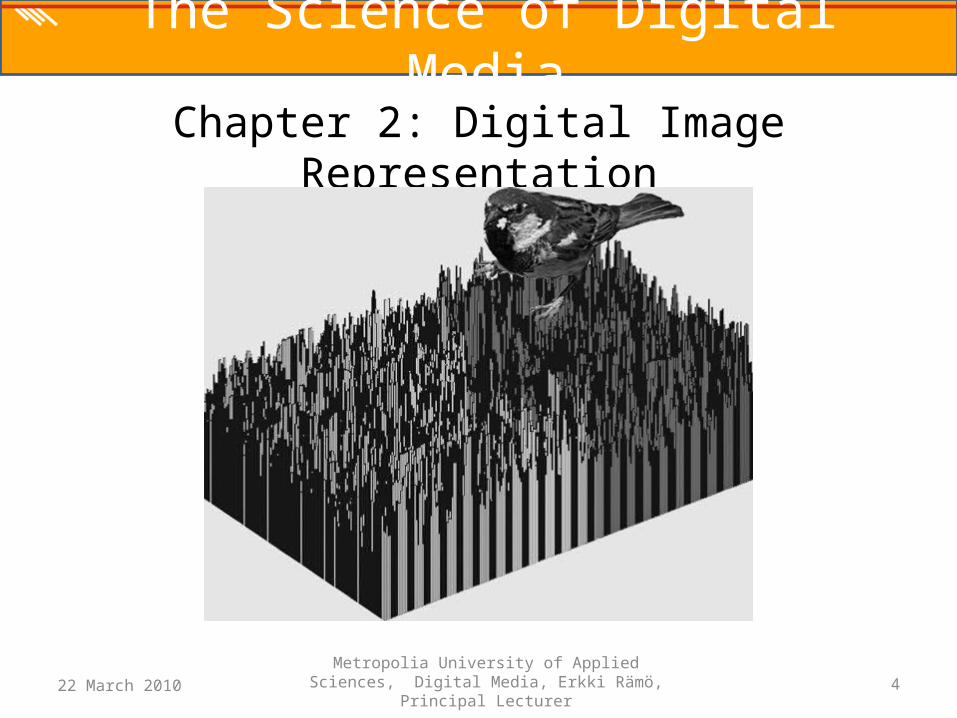
The Science of Digital MediaChapter 2: Digital Image Representation
22 March 2010 4Metropolia University of Applied Sciences, Digital
Media, Erkki Rämö, Principal Lecturer
The Science of Digital Media
The Science of Digital Media
• Digital images are created by three basic methods: – Bitmapping, – Vector graphics, and – Procedural modeling
Introduction
22 March 2010 5Metropolia University of Applied Sciences, Digital
Media, Erkki Rämö, Principal Lecturer
The Science of Digital Media

The Science of Digital Media
• A bitmap is two-dimensional array of pixels describing a digital image
• Each pixel, short for picture element, is a number representing the color at position (r,c) in the bitmap, where “r” is the row and “c” is the column
22 March 2010 6Metropolia University of Applied Sciences, Digital
Media, Erkki Rämö, Principal Lecturer
Bitmap Definition
2.2 - Bitmaps

The Science of Digital Media
• There are three ways to create a bitmap:– First, through software, by means of a paint program– Second, through reproduction scenes and objects we
perceive in the world around us– Third, through shooting the image with a digital camera
and transfer the bitmap to your computer
• In this course the emphasis will be on bitmap images created from digital photography
22 March 2010 7Metropolia University of Applied Sciences, Digital
Media, Erkki Rämö, Principal Lecturer
Bitmap Digitization (1)
2.2 - Bitmaps

The Science of Digital Media
• Through software, by means of a paint program– you paint your picture one pixel at a time,
• Through reproduction scenes and objects we perceive in the world around us– take a snapshot with a traditional analog camera, develop a
film and then scan the photograph with a digital scanner to create a bitmap image that can be stored on your computer
• Through shooting the image with a digital camera and transfer the bitmap to your computer– Digital cameras can have various kinds of memory cards,
sometimes called flash memory on which the digital image can be stored
22 March 2010 8Metropolia University of Applied Sciences, Digital
Media, Erkki Rämö, Principal Lecturer
Bitmap Digitization (2)
2.2 - Bitmaps
The Science of Digital Media
• Digital camera uses the same digitization process discussed in part-I (sampling and quantization)
• Sampling rate for digital camera– How many points of color are sampled and recorded in
each dimension of the image– For example: 1600 x 1200, 1280 x 960, 1024 x 768 and
640 x 480. Some cameras do offer no choice
22 March 2010 9Metropolia University of Applied Sciences, Digital
Media, Erkki Rämö, Principal Lecturer
Bitmap Digitization – Sampling
2.2 - Bitmaps
The Science of Digital Media
• Quantization in digital camera– Is a matter of the color model used and the
corresponding bit depth (color models will be dealt in more details later in this chapter)
– For now the digital cameras generally use RGB color, which saves each pixel in three bytes one for each of the color channels: red(R), green(G) and blue(B)
– A higher bit depth is possible in RGB, but three bytes per pixel is common. 3 bytes = 24bits, therefore, 224 = 16,777,216 colors to be represented
22 March 2010 10Metropolia University of Applied Sciences, Digital
Media, Erkki Rämö, Principal Lecturer
Bitmap Digitization - Quantization
2.2 - Bitmaps

The Science of Digital Media
• Both quantization and digitization can introduce error– The image captured might not represent, with perfect
fidelity, the original scene or objects that were photographed
– If you do not take enough samples over the area being captured, the image will lack clarity
– The larger the area represented by a pixel, the blurrier the picture, because sabtle transition from one color to the next cannot be captured
22 March 2010 11Metropolia University of Applied Sciences, Digital
Media, Erkki Rämö, Principal Lecturer
Quantization and Digitization Error (1)
2.2 - Bitmaps
The Science of Digital Media
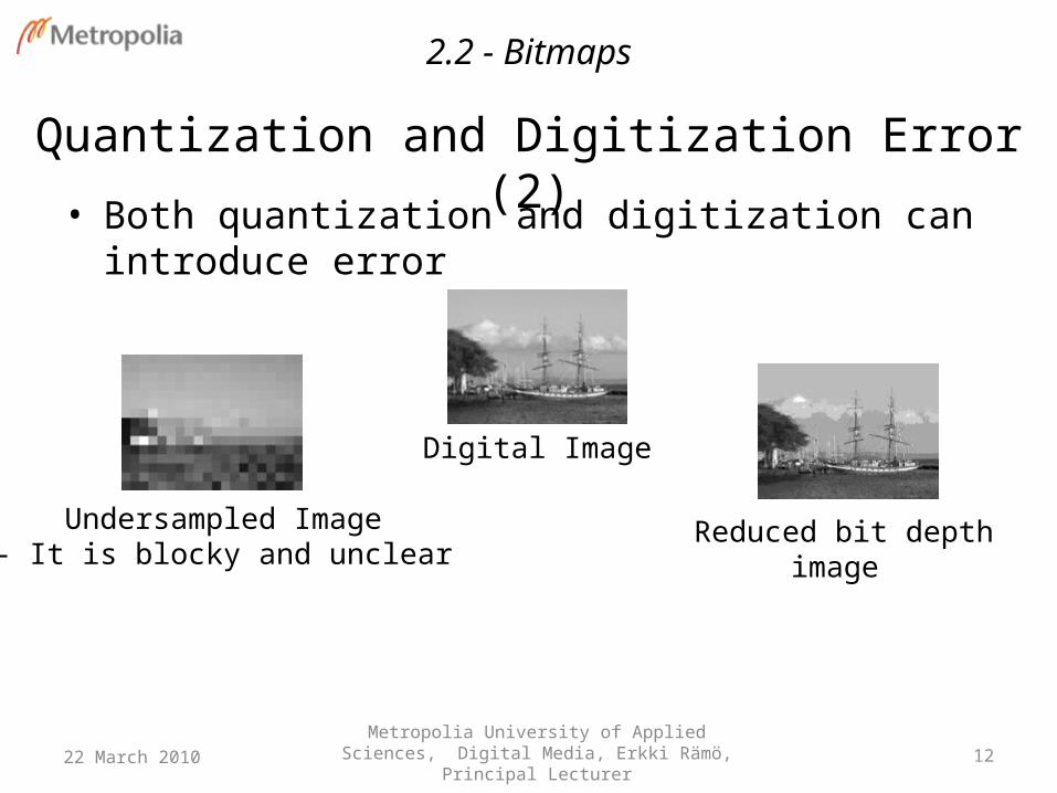
• Both quantization and digitization can introduce error
22 March 2010 12Metropolia University of Applied Sciences, Digital
Media, Erkki Rämö, Principal Lecturer
Quantization and Digitization Error (2)
Digital Image
Undersampled Image- It is blocky and unclear
Reduced bit depth image
2.2 - Bitmaps

The Science of Digital Media
• We have defined pixel in context of bitmap, but has another meaning in the context of a computer display
• Pixel in Computer Display context– Is a physical object a point of light on the screen
• Sometimes logical pixel and physical pixel are used to distinguish between the two usages
• When you display a bitmap image on your computer:– The logical pixel i.e., the number representing a color
and stored for a given position in the image file is mapped to a physical pixel on the computer screen
22 March 2010 13Metropolia University of Applied Sciences, Digital
Media, Erkki Rämö, Principal Lecturer
Pixel Dimension, Resolution and Image Size
2.2 - Bitmaps
The Science of Digital Media
• Is a number of pixels horizontally (i.e., width, “w”) and vertically (i.e., height, “h”) denoted w x h
• For example: Digital camera can take digital images with pixel dimensions of 1600 x 1200. Similarly, your computer screen has a fixed maximum pixel dimension e.g., of 1024 x 768 or 1400 x 1050– Megapixels concept in digital cameras
• Is a value derived from the maximum pixel dimensions allowable for pictures taken with the camera.
• Example : If the largest picture you can take in pixels for a certain camera is 2048 x 1536, i.e., 3,145,728 total pixels, then this is a 3 Megapixel camera (approximately)
22 March 2010 14Metropolia University of Applied Sciences, Digital
Media, Erkki Rämö, Principal Lecturer
Pixel Dimension
2.2 - Bitmaps

The Science of Digital Media
• Is the number of pixels in an image file per unit of spatial measure, i.e., pixel per inch, ppi
• It is assumed that the same number of pixels are used in the horizontal and vertical directions
• Resolution of a printer is a matter of how many dots of color it can print over an area, i.e., dots per inch (DPI)
• The printer and its software map the pixels in an images file to the dots of color printed
• There maybe more or fewer pixels per inch than dots printed
22 March 2010 15Metropolia University of Applied Sciences, Digital
Media, Erkki Rämö, Principal Lecturer
Resolution
2.2 - Bitmaps
The Science of Digital Media
• Is a physical dimensions of an image when it is printed our or displayed on a computer, e.g., in inches or centimeters
• By this definition image size is a function of the pixel dimension and resolution, as follows:– For an image with resolution “r” and pixel dimensions “w x
h” where “w” is the width and “h” is the height, the printed image size “a x b” is given by:
– Example: If you have an image that is 1600 x 1200, and you choose to print it out at 200ppi, it will be 8” x 6”
22 March 2010 16Metropolia University of Applied Sciences, Digital
Media, Erkki Rämö, Principal Lecturer
rhbandr
wa
Image Size - On Print
2.2 - Bitmaps
The Science of Digital Media
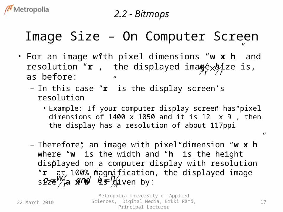
• For an image with pixel dimensions “w x h” and resolution “r”, the displayed image size is, as before:– In this case “r” is the display screen’s resolution
• Example: If your computer display screen has pixel dimensions of 1400 x 1050 and it is 12” x 9”, then the display has a resolution of about 117ppi
– Therefore, an image with pixel dimension “w x h” where “w” is the width and “h” is the height displayed on a computer display with resolution “r” at 100% magnification, the displayed image size “a x b” is given by:
22 March 2010 17Metropolia University of Applied Sciences, Digital
Media, Erkki Rämö, Principal Lecturer
rh
rw
Image Size – On Computer Screen
rhbandr
wa
2.2 - Bitmaps

The Science of Digital Media
• Image Cropping is simply cutting off part of the picture, discarding the unwanted pixels
• Resampling is changing the number of pixels in an image– Upsampling: increasing the pixel dimensions– Downsampling: decreasing the pixel dimensions– Resampling always involves some kind of interpolation,
averaging or estimation and thus it cannot improve the quality of an image
22 March 2010 18Metropolia University of Applied Sciences, Digital
Media, Erkki Rämö, Principal Lecturer
Image Size – Common Terms
2.2 - Bitmaps
The Science of Digital Media
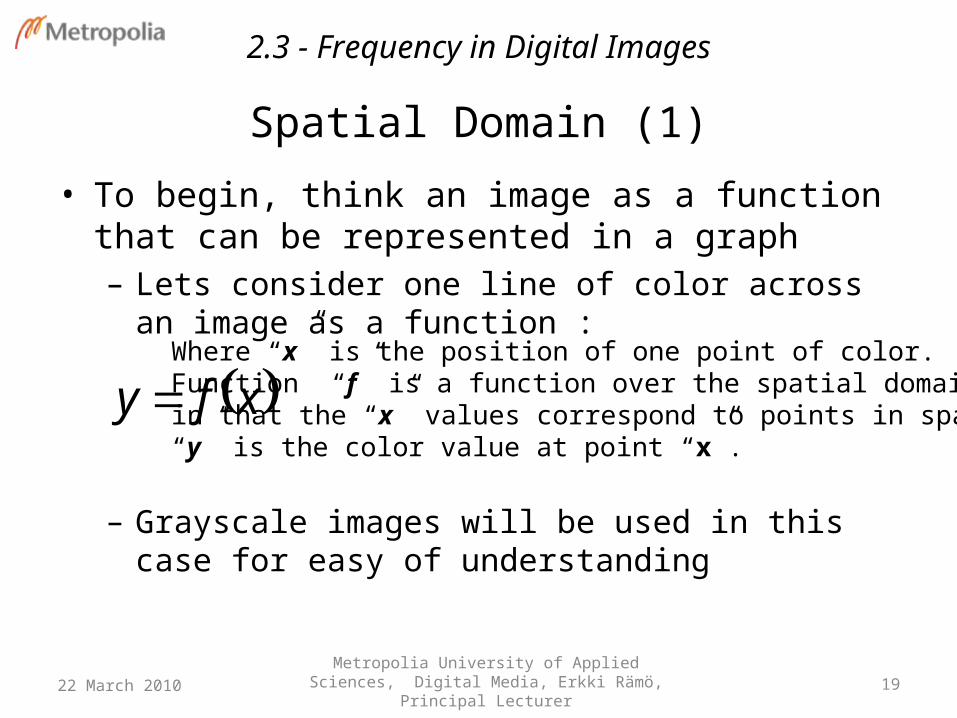
• To begin, think an image as a function that can be represented in a graph– Lets consider one line of color across an image as a
function :
– Grayscale images will be used in this case for easy of understanding
22 March 2010 19Metropolia University of Applied Sciences, Digital
Media, Erkki Rämö, Principal Lecturer
xfy Where “x” is the position of one point of color.Function “f” is a function over the spatial domainin that the “x” values correspond to points in space.“y” is the color value at point “x”.
Spatial Domain (1)
2.3 - Frequency in Digital Images

The Science of Digital Media
• In digital images, frequency refers to the rate at which color value changes
22 March 2010 20Metropolia University of Applied Sciences, Digital
Media, Erkki Rämö, Principal Lecturer
Spatial Domain (2)
Figure 2.4: A image in which color varies continuously from light gray
to dark gray and back again
Figure 2.5: Graph of function y=f(x) for one line of color across the image. f is
assumed to be continuous and periodic
2.3 - Frequency in Digital Images
The Science of Digital Media
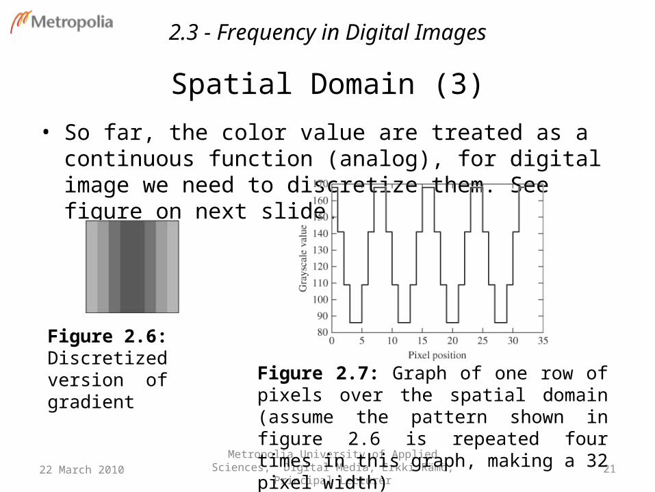
• So far, the color value are treated as a continuous function (analog), for digital image we need to discretize them. See figure on next slide.
22 March 2010 21Metropolia University of Applied Sciences, Digital
Media, Erkki Rämö, Principal Lecturer
Spatial Domain (3)
Figure 2.6: Discretized version of gradient
Figure 2.7: Graph of one row of pixels over the spatial domain (assume the pattern shown in figure 2.6 is repeated four times in this graph, making a 32 pixel width)
2.3 - Frequency in Digital Images

The Science of Digital Media
• All bitmap images, even those with irregular pattern of pixel values like the picture of the sparrow, can be viewed as waveform
22 March 2010 22Metropolia University of Applied Sciences, Digital
Media, Erkki Rämö, Principal Lecturer
Spatial Domain (4)
Figure 2.8: Grayscale bitmap image of sparrow
Figure 2.9: Graph of one row of sparrow bitmap over the spatial domain
2.3 - Frequency in Digital Images

The Science of Digital Media
• Extending these observations to two-dimensional image is straight forward
22 March 2010 23Metropolia University of Applied Sciences, Digital
Media, Erkki Rämö, Principal Lecturer
Spatial Domain (5)
Figure 2.10: Graph of Figure 2.6, assumed to be an 8 × 8 bitmap image
Figure 2.11: Graph of two-dimensional bitmap of sparrow (figure 2.8)
2.3 - Frequency in Digital Images
The Science of Digital Media
• All the previous graphs have been presented in the spatial domain
• To separate out individual frequency components, we need to translate the image into frequency domain
• According to Fourier theory:– Any complex periodic waveform can be equated to an
infinite sum of simple sinusoidal waves of varying frequencies and amplitudes
22 March 2010 24Metropolia University of Applied Sciences, Digital
Media, Erkki Rämö, Principal Lecturer
Frequency Domain (1)
2.3 - Frequency in Digital Images
The Science of Digital Media
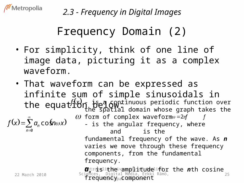
• For simplicity, think of one line of image data, picturing it as a complex waveform.
• That waveform can be expressed as infinite sum of simple sinusoidals in the equation below:
22 March 2010 25Metropolia University of Applied Sciences, Digital
Media, Erkki Rämö, Principal Lecturer
0
cosn
n xnaxf
- is a continuous periodic function over the spatial domain whose graph takes the form of complex waveform- is the angular frequency, where and is thefundamental frequency of the wave. As n varies we move through these frequency components, from the fundamental frequency.an is the amplitude for the nth cosine frequency component
xf
f 2 f
Frequency Domain (2)
2.3 - Frequency in Digital Images
The Science of Digital Media
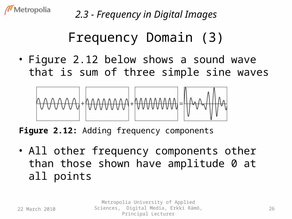
• Figure 2.12 below shows a sound wave that is sum of three simple sine waves
• All other frequency components other than those shown have amplitude 0 at all points
22 March 2010 26Metropolia University of Applied Sciences, Digital
Media, Erkki Rämö, Principal Lecturer
Frequency Domain (3)
Figure 2.12: Adding frequency components
2.3 - Frequency in Digital Images
The Science of Digital Media
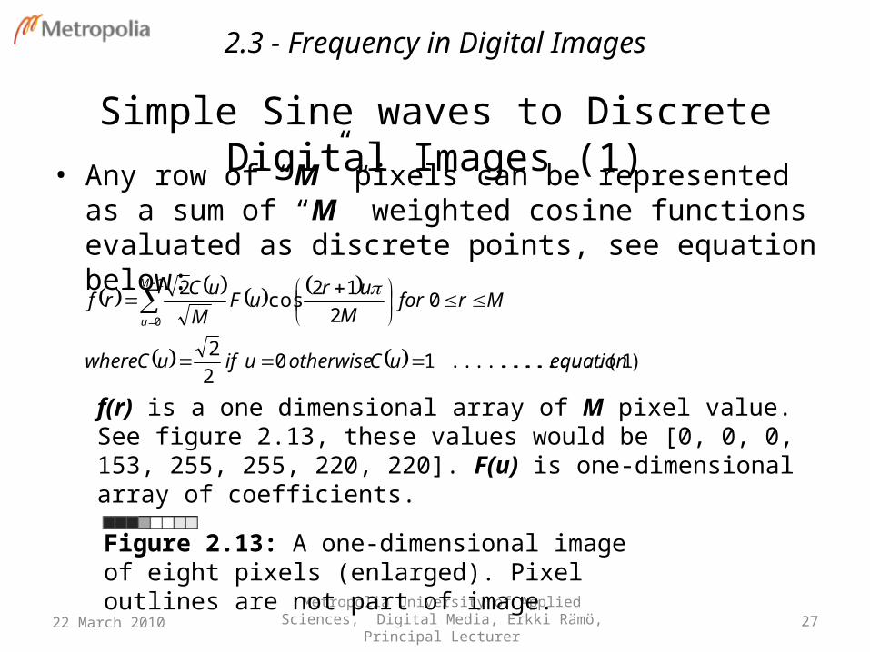
• Any row of “M” pixels can be represented as a sum of “M” weighted cosine functions evaluated as discrete points, see equation below:
22 March 2010 27Metropolia University of Applied Sciences, Digital
Media, Erkki Rämö, Principal Lecturer
Simple Sine waves to Discrete Digital Images (1)
)1.........(..........102
2
02
12cos
21
0
equationuCotherwiseuifuCwhere
MrforM
uruF
M
uCrf
M
u
f(r) is a one dimensional array of M pixel value. See figure 2.13, these values would be [0, 0, 0, 153, 255, 255, 220, 220]. F(u) is one-dimensional array of coefficients.
Figure 2.13: A one-dimensional image of eight pixels (enlarged). Pixel outlines are not part of image.
2.3 - Frequency in Digital Images

The Science of Digital Media
• Each function is called a basis function• You can also think of each function as a frequency
component• The coefficients in F(u) tells how much each
frequency component is weighted in the sum that produces the pixel value
• You can think of this as “how much” each frequency component contributes to the image
22 March 2010 28Metropolia University of Applied Sciences, Digital
Media, Erkki Rämö, Principal Lecturer
M
ur
2
12cos
Simple Sine waves to Discrete Digital Images (2)
2.3 - Frequency in Digital Images

The Science of Digital Media
• For M = 8, the basic functions are those given in the figures below
• As the values of cosine function decrease, the pixels gets darker: 1 represent white and -1 black
22 March 2010 29Metropolia University of Applied Sciences, Digital
Media, Erkki Rämö, Principal Lecturer
Simple Sine waves to Discrete Digital Images (3)
Figure 2.14: Basis Function 0
Figure 2.15: Basis Function 1
2.3 - Frequency in Digital Images

The Science of Digital Media
22 March 2010 30Metropolia University of Applied Sciences, Digital
Media, Erkki Rämö, Principal Lecturer
Simple Sine waves to Discrete Digital Images (4)
Figure 2.16: Basis Function 2
Figure 2.17: Basis Function 3
Figure 2.18: Basis Function 4
2.3 - Frequency in Digital Images

The Science of Digital Media
22 March 2010 31Metropolia University of Applied Sciences, Digital
Media, Erkki Rämö, Principal Lecturer
Figure 2.19: Basis Function 5
Figure 2.20: Basis Function 6
Figure 2.21: Basis Function 7
Simple Sine waves to Discrete Digital Images (5)
2.3 - Frequency in Digital Images
The Science of Digital Media
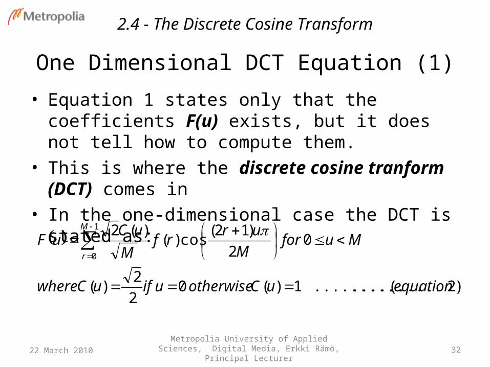
• Equation 1 states only that the coefficients F(u) exists, but it does not tell how to compute them.
• This is where the discrete cosine tranform (DCT) comes in
• In the one-dimensional case the DCT is stated as:
22 March 2010 32Metropolia University of Applied Sciences, Digital
Media, Erkki Rämö, Principal Lecturer
)2(....................1)(02
2)(
02
)12(cos)(
)(21
0
equationuCotherwiseuifuCwhere
MuforM
urrf
M
uCuF
M
r
One Dimensional DCT Equation (1)
2.4 - The Discrete Cosine Transform

The Science of Digital Media
• The DCT equation2 tells how to transform an image from the spatial domain, which gives color or gray values to frequency domain which gives coefficients by which the frequency components should be multiplied
• Example for DCT Equation 2 (a):– Consider the row of 8-pixels (seen previously) with
corresponding grayscale values [0, 0, 0, 153, 255, 255, 220, 220]– This array represents the image in the spatial domain. – If you compute a value F(u) for using equation2,
you get the array of values [389.97, -280.13, -93.54, 83.38, 54.09, -20.51, -19.80, -16.34]
22 March 2010 33Metropolia University of Applied Sciences, Digital
Media, Erkki Rämö, Principal Lecturer
10 Mu
One Dimensional DCT Equation (2)
2.4 - The Discrete Cosine Transform

The Science of Digital Media
• Example for Equation 2 (b):– You have applied the DCT, yielding an array that
represents the pixels in the frequency domain– This means the line of pixels is a linear combination of
frequency components, i.e., the basis function multiplied by the coefficients in “F” and a constant added together, as follows:
22 March 2010 34Metropolia University of Applied Sciences, Digital
Media, Erkki Rämö, Principal Lecturer
M
r
M
r
M
r
M
r
M
r
M
r
M
r
MMrf
2
7)12(cos34.16
2
6)12(cos80.19
2
5)12(cos51.20
2
4)12(cos09.54
2
3)12(cos38.83
2
2)12(cos54.93
2
)12(cos13.280
2)0cos(
97.389)(
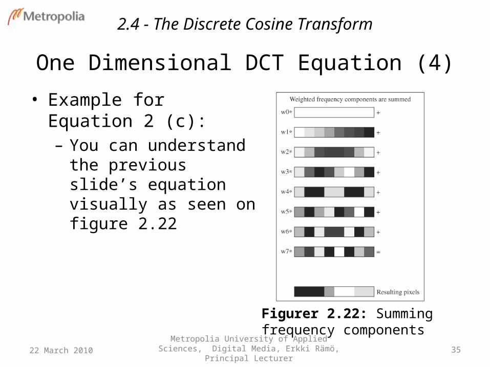
One Dimensional DCT Equation (3)
2.4 - The Discrete Cosine Transform
The Science of Digital Media
• Example for Equation 2 (c):– You can understand the
previous slide’s equation visually as seen on figure 2.22
22 March 2010 35Metropolia University of Applied Sciences, Digital
Media, Erkki Rämö, Principal Lecturer
Figurer 2.22: Summing frequency components
One Dimensional DCT Equation (4)
2.4 - The Discrete Cosine Transform

The Science of Digital Media
• Example for Equation 2 (d):– Having a negative coefficient for a frequency
components amounts to adding the inverted waveform, as shown in Figure 2.23
22 March 2010 36Metropolia University of Applied Sciences, Digital
Media, Erkki Rämö, Principal Lecturer
Figure 2.23: A frequency component with a negative coefficient
One Dimensional DCT Equation (5)
2.4 - The Discrete Cosine Transform

The Science of Digital Media
• First element F(0) is called the DC component (for a periodic function, represented in the frequency domain, the DC component is a scaled average value of the waveform)
• You can see this in the one-dimensional case:
22 March 2010 37Metropolia University of Applied Sciences, Digital
Media, Erkki Rämö, Principal Lecturer
)7()6()5()4(
)3()2()1()0(1
)7()0cos()6()0cos()5()0cos()4()0cos(
)3()0cos()2()0cos()1()0cos()0()0cos(1)0(
ffff
ffff
M
ffff
ffff
MF
One Dimensional DCT Equation – Terminologies (1)
2.4 - The Discrete Cosine Transform

The Science of Digital Media
• All the other components (F(1) through F(M-1)) are called AC components.
• The names were derived from an analogy with electrical systems, the DC component being comparable to direct current and AC component being comparable to alternating current
22 March 2010 38Metropolia University of Applied Sciences, Digital
Media, Erkki Rämö, Principal Lecturer
One Dimensional DCT Equation – Terminologies (2)
2.4 - The Discrete Cosine Transform

The Science of Digital Media
• We have been looking only at one-dimensional case to keep things simple. But to present images we need two dimensions.
• The two dimensional DCT is expressed as:– Let f(r,s) be the pixel value at row r and column s of a
bitmap. F(u,v) is the coefficient of the frequency component at (u,v), where
22 March 2010 39Metropolia University of Applied Sciences, Digital
Media, Erkki Rämö, Principal Lecturer
1,01,0 NvsandMur
1)(02
2)(
2
)12(cos
2
)12(cos),(
)()(2),(
1
0
1
0
CotherwiseifCwhere
N
vs
M
ursrf
MN
vCuCvuF
M
r
N
s
Two Dimensional DCT Equation (1)
2.4 - The Discrete Cosine Transform

The Science of Digital Media
• Matrices are assumed to be treated in row-major order, i.e., row by row rather than column by column
• You can think of DCT in two equivalent ways:– Think of the DCT as taking a function over the spatial
domain, i.e., function f(r,s), and then returning a function over the frequency domain, i.e., function f(u,v)
– Think of the DCT as taking a bitmap image in the form of a matrix of color values – f(r,s) and returning the frequency components of the bitmap in the form of matrix of coefficients – f(u,v).
22 March 2010 40Metropolia University of Applied Sciences, Digital
Media, Erkki Rämö, Principal Lecturer
Two Dimensional DCT Equation (2)
2.4 - The Discrete Cosine Transform

The Science of Digital Media
• Rather than being applied to a full M x N image, the DCT is applied to 8 x 8 pixel subblocks
• This discussion will be limited to image in these dimensins (i.e., 8 x 8 pixel subblocks)
22 March 2010 41Metropolia University of Applied Sciences, Digital
Media, Erkki Rämö, Principal Lecturer
Two Dimensional DCT Equation (3)
Figure 2.24 - 8 x 8 bitmap image. Pixel outlines are not part of image
2.4 - The Discrete Cosine Transform

The Science of Digital Media
22 March 2010 42Metropolia University of Applied Sciences, Digital
Media, Erkki Rämö, Principal Lecturer
Two Dimensional DCT Equation (4)• Tables showing color value for Image in Figure 2.24 and its Amplitude of Frequency components
2.4 - The Discrete Cosine Transform
The Science of Digital Media
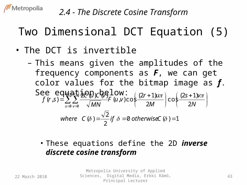
• The DCT is invertible– This means given the amplitudes of the frequency
components as F, we can get color values for the bitmap image as f. See equation below:
• These equations define the 2D inverse discrete cosine transform
22 March 2010 43Metropolia University of Applied Sciences, Digital
Media, Erkki Rämö, Principal Lecturer
1)(02
2)(
2
)12(cos
2
)12(cos),(
)()(2),(
1
0
1
0
CotherwiseifCwhere
N
vs
M
urvuF
MN
vCuCsrf
M
u
N
v
Two Dimensional DCT Equation (5)
2.4 - The Discrete Cosine Transform
The Science of Digital Media
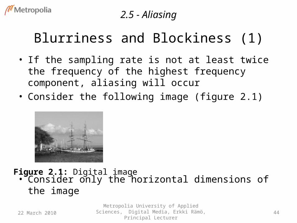
• If the sampling rate is not at least twice the frequency of the highest frequency component, aliasing will occur
• Consider the following image (figure 2.1)
• Consider only the horizontal dimensions of the image
22 March 2010 44Metropolia University of Applied Sciences, Digital
Media, Erkki Rämö, Principal Lecturer
Blurriness and Blockiness (1)
2.5 - Aliasing
Figure 2.1: Digital image

The Science of Digital Media
• Imagine that the picture has been divided into sampling areas so that only 15 samples are taken across a row (very low rate)
• If the color changes even one time within one of the sample areas, then the two colors in that area can not both be represented by the sample
• This implies that the image reconstructed from the sample will not be a perfect reproduction of the original scene, as seen in the figure below
22 March 2010 45Metropolia University of Applied Sciences, Digital
Media, Erkki Rämö, Principal Lecturer
Blurriness and Blockiness (2)
2.5 - Aliasing
The Science of Digital Media
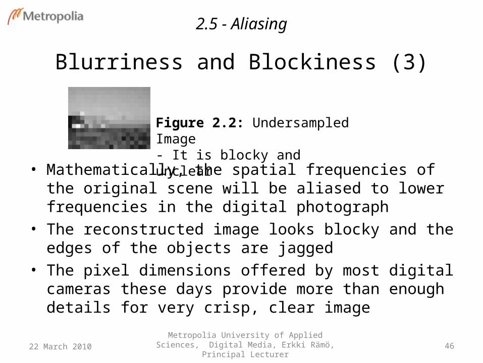
• Mathematically, the spatial frequencies of the original scene will be aliased to lower frequencies in the digital photograph
• The reconstructed image looks blocky and the edges of the objects are jagged
• The pixel dimensions offered by most digital cameras these days provide more than enough details for very crisp, clear image
22 March 2010 46Metropolia University of Applied Sciences, Digital
Media, Erkki Rämö, Principal Lecturer
Blurriness and Blockiness (3)
Figure 2.2: Undersampled Image- It is blocky and unclear
2.5 - Aliasing

The Science of Digital Media
• Moiré effect or moiré pattern is another interesting example of aliasing– Can occur when there is a pattern in the image being
photographed, and the sampling rate for the digital image is not enough to capture the frequency of the pattern
22 March 2010 47Metropolia University of Applied Sciences, Digital
Media, Erkki Rämö, Principal Lecturer
Moiré Patterns (1)
2.5 - Aliasing

The Science of Digital Media
• What would happen if we sampled this image five time, at a regular spaced intervals?– Depending on where the sampling
started, the resulting image would be either all black or all white
– If we sample more that ten times (more than twice per repetition of the pattern), we will be able to reconstruct the image faithfully. This is a simple application of Nyquist Theorem.
22 March 2010 48Metropolia University of Applied Sciences, Digital
Media, Erkki Rämö, Principal Lecturer
Moiré Patterns (2)
A simple image with vertical stripes
Figure 2.29
2.5 - Aliasing
The Science of Digital Media
• More visually interesting moiré effects can result when the original pattern is more complex and the pattern is tilted at an angle with respect to the sampling
• Assume that if more than half a sampling block is filled with black from the original striped image, then that block becomes black. Otherwise, it is white.
22 March 2010 49Metropolia University of Applied Sciences, Digital
Media, Erkki Rämö, Principal Lecturer
Moiré Patterns (3)
2.5 - Aliasing

The Science of Digital Media
• The pattern in the reconstructed image is distorted in a moiré effect, see figure 2.30
• Moiré patterns can result both when a digital photograph is taken and when a picture is scanned, because both processes involve choosing a sampling rate.
Figure 2.30: Sampling that can result in a moiré pattern
22 March 2010 50Metropolia University of Applied Sciences, Digital
Media, Erkki Rämö, Principal Lecturer
Moiré Patterns (4)
2.5 - Aliasing
The Science of Digital Media
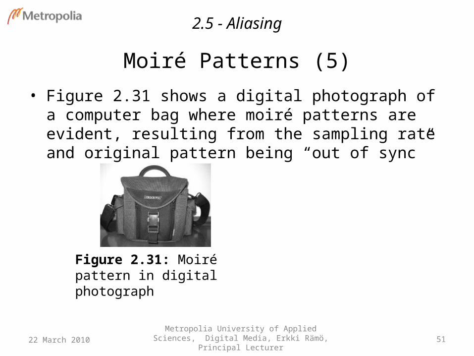
• Figure 2.31 shows a digital photograph of a computer bag where moiré patterns are evident, resulting from the sampling rate and original pattern being “out of sync”
Figure 2.31: Moiré pattern in digital photograph
22 March 2010 51Metropolia University of Applied Sciences, Digital
Media, Erkki Rämö, Principal Lecturer
Moiré Patterns (5)
2.5 - Aliasing
The Science of Digital Media
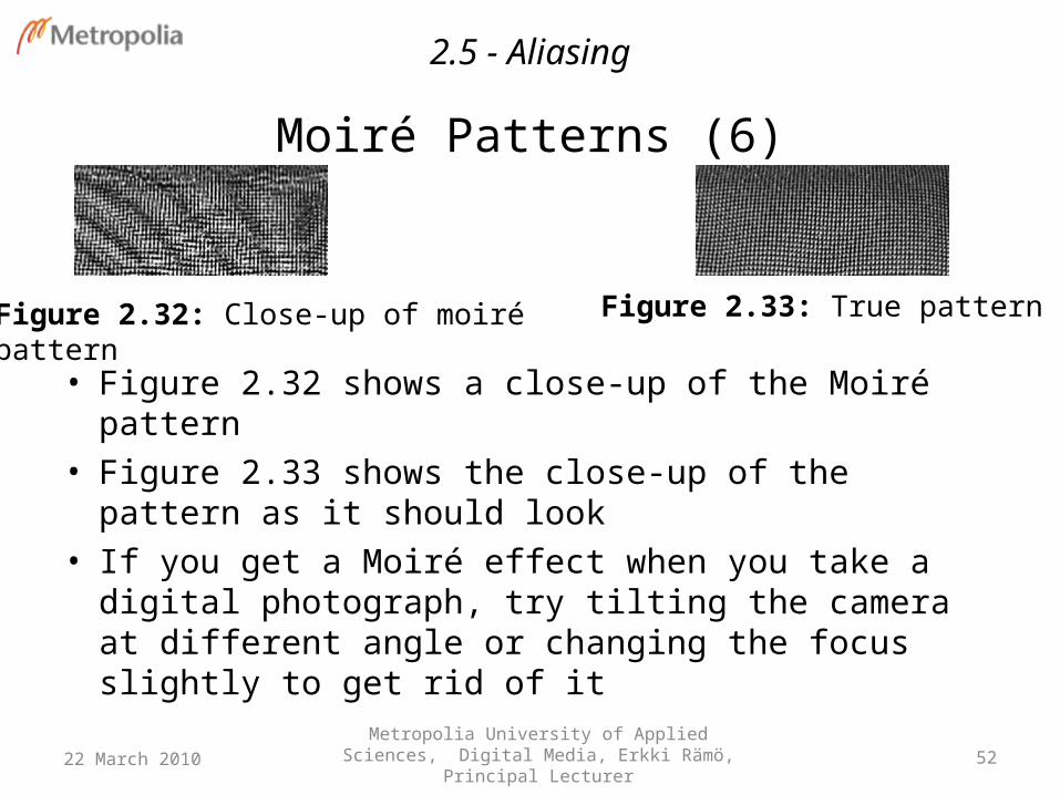
• Figure 2.32 shows a close-up of the Moiré pattern• Figure 2.33 shows the close-up of the pattern as it
should look• If you get a Moiré effect when you take a digital
photograph, try tilting the camera at different angle or changing the focus slightly to get rid of it
22 March 2010 52Metropolia University of Applied Sciences, Digital
Media, Erkki Rämö, Principal Lecturer
Moiré Patterns (6)
Figure 2.32: Close-up of moiré pattern
Figure 2.33: True pattern
2.5 - Aliasing
The Science of Digital Media
• Camera tilting or refocusing will change the sampling orientation or sampling precision with respect to the pattern
• Moiré patterns occur in digital photography because it is based on discrete samples
• An alias of the original pattern results if the discrete samples are taken “off beat” from the detailed pattern in the subject being photographed
• But this does not fully explain the source of the problem
22 March 2010 53Metropolia University of Applied Sciences, Digital
Media, Erkki Rämö, Principal Lecturer
Moiré Patterns (7)
2.5 - Aliasing
The Science of Digital Media
• Sometimes aliasing in digital images manifest itself as small area of incorrect colors or artificial auras around objects, which can be referred to as– Color aliasing – Moiré fringes– False coloration– Phantom colors
• To understand what causes this phenomenon, you have to know a little about how color is perceived and recorded in digital camera
22 March 2010 54Metropolia University of Applied Sciences, Digital
Media, Erkki Rämö, Principal Lecturer
Area of Incorrect Colors
2.5 - Aliasing
The Science of Digital Media
• Photograph taken with a traditional analog camera– Film that is covered with silver-laden is exposed to light– There are three layers on photographic film, one
sensitive to red, one to green and one to blue light (assuming the use of RGB color)
– At each point across a continuous plane, all three color components are sensed simultaneously
– The degree to which the silver atoms gather together measures the amount of light to which the film is exposed
22 March 2010 55Metropolia University of Applied Sciences, Digital
Media, Erkki Rämö, Principal Lecturer
Analog Camera Photography
2.5 - Aliasing
The Science of Digital Media
• Analogy photography measures the incident light continuously across the focal plane while digital photography samples it only at discrete points.
• Another difference is that it is more difficult for digital camera to sense all three color components i.e., red, green and blue at each sample point.– The constraints on sampling color and the use of
interpolation to “fill the blanks” in digital sampling can lead to color aliasing.
22 March 2010 56Metropolia University of Applied Sciences, Digital
Media, Erkki Rämö, Principal Lecturer
Analog Versus Digital Photography
2.5 - Aliasing

The Science of Digital Media
• Many current digital cameras use charge-coupled device (CCD) technology to sense light and thereby color
• CMOS-Complementary Metal-Oxide Semiconductor is an alternative technology for digital photography
• CCD– Consists of two-dimensional array of photosites– Each photosite correspond to one sample (one pixel in
the digital image)– The number of photosites determines the limits of
camera’s resolution22 March 2010 57
Metropolia University of Applied Sciences, Digital Media, Erkki Rämö, Principal Lecturer
Charge-Coupled Device (CCD) - 1
2.5 - Aliasing

The Science of Digital Media
• To sense red, green or blue at a discrete point, the sensor at that photosite is covered with red, green or blue color filter
• But the question is:– Should all three color components be sensed simultaneously
at each photosite?– Should they be sensed at different moments when the picture
is taken?– Or should only one color component per photosite be
sensed?
• There are various CCD designs in current technology each with its own advantages and disadvantages
22 March 2010 58Metropolia University of Applied Sciences, Digital
Media, Erkki Rämö, Principal Lecturer
Charge-Coupled Device (CCD) - 2
2.5 - Aliasing
The Science of Digital Media
• The incident light can be divided into three beams– Three sensors are used at each photosite, each covered
with a filter that allows only red, green or blue to be sensed.
– Is an expensive solution and creates a bulkier camera
• The sensor is can be rotated when the picture is taken so that it takes in information about red, green and blue light in succession– The three colors are not sensed at precisely the same
moment, so the subject being photographed needs to be still
22 March 2010 59Metropolia University of Applied Sciences, Digital
Media, Erkki Rämö, Principal Lecturer
Charge-Coupled Device (CCD) - 3
2.5 - Aliasing
The Science of Digital Media
• A more recently developed technology (Foveon X3) uses silicon for the sensors in a method called vertical stacking.– Different depths of silicon absorb different wavelengths of
light, all three color components can be detected at one photosite.
– This technology is gaining popularity
• A less expensive method of color detection uses a color array to detect only one color component at each photosite– Interpolation is then used to derive the other two color
components based on information from neighbouring sites– It is the interpolation that can lead to color aliasing
22 March 2010 60Metropolia University of Applied Sciences, Digital
Media, Erkki Rämö, Principal Lecturer
Charge-Coupled Device (CCD) - 4
2.5 - Aliasing
The Science of Digital Media
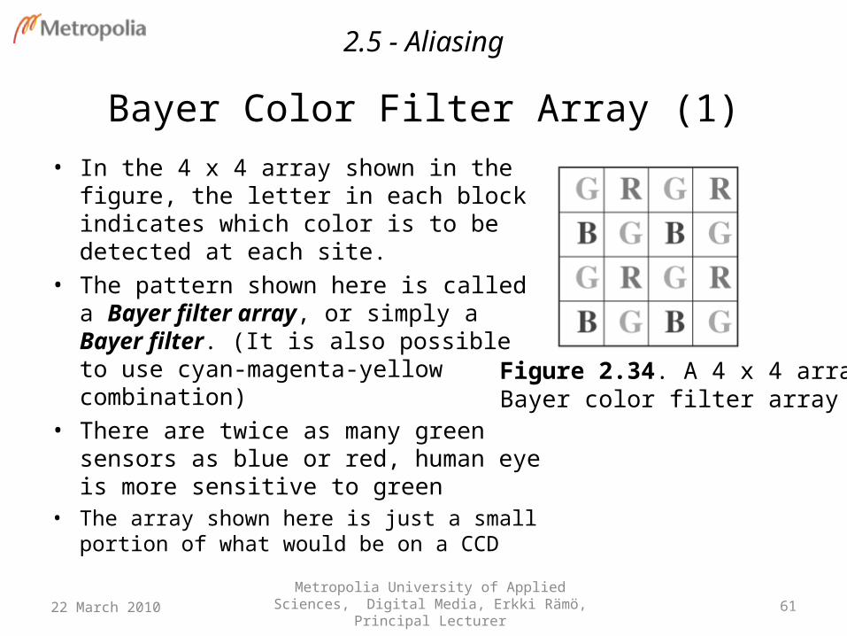
• In the 4 x 4 array shown in the figure, the letter in each block indicates which color is to be detected at each site.
• The pattern shown here is called a Bayer filter array, or simply a Bayer filter. (It is also possible to use cyan-magenta-yellow combination)
• There are twice as many green sensors as blue or red, human eye is more sensitive to green
• The array shown here is just a small portion of what would be on a CCD
22 March 2010 61Metropolia University of Applied Sciences, Digital
Media, Erkki Rämö, Principal Lecturer
Bayer Color Filter Array (1)
Figure 2.34. A 4 x 4 array;Bayer color filter array
2.5 - Aliasing

The Science of Digital Media
• Each block in the array represents a photosite, and each photosite has a filter on it that determines which color is sensed at that site
• The interpolation algorithm for deriving the two missing color channels at each photosite is called demosaicing
• A variety of demosaicing algorithms have been devised
• A simple nearest neighbor algorithm determines a missing color “c” for a photosite based on the colors of the neighbors that have color “c”
22 March 2010 62Metropolia University of Applied Sciences, Digital
Media, Erkki Rämö, Principal Lecturer
Bayer Color Filter Array (2)
Figure 2.34. A 4 x 4 array;Bayer color filter array
2.5 - Aliasing

The Science of Digital Media
• For the algorithm given below, assuming a CCD array of dimensions (m x n), the nearest neighbors of photosite (i, j) are sites:– (i-1, j-1), (i-1, j), (i-1, j+1), (i, j-1), (i, j+1), (i+1, j-1), (i+1, j),
(i+1, j+1)
where 0 ≤ j ≤ n (disregarding boundary areas where neighbors may not exist)
22 March 2010 63Metropolia University of Applied Sciences, Digital
Media, Erkki Rämö, Principal Lecturer
Nearest Neighbor Algorithm
2.5 - Aliasing

The Science of Digital Media
• With this algorithm, there may be either two or four neighbors involved in the averaging as shown in Figure 2.35a and Figure 2.35b
22 March 2010 64Metropolia University of Applied Sciences, Digital
Media, Erkki Rämö, Principal Lecturer
Photosite Interpolation (1)
Figure 2.35 Photosite Interpolation
2.5 - Aliasing

The Science of Digital Media
• Other standard interpolation methods are Linear, Cubic , Cubic spline etc
• The region of the nearest neighbors can be larger than 3 x 3 or a shap other than a square
• The result of interpolation is the formation of full RGB color channels to the two photosites using the information from one of them
• Most digital camera that uses CCD technology uses this method
22 March 2010 65Metropolia University of Applied Sciences, Digital
Media, Erkki Rämö, Principal Lecturer
Photosite Interpolation (2)
2.5 - Aliasing

The Science of Digital Media
• Interpolation by its nature cannot give a perfect reproduction of the scene being photographed
• Occasionally color aliasing results from the process, detected as Moiré patterns, streaks or spots of color not present in the original scene
22 March 2010 66Metropolia University of Applied Sciences, Digital
Media, Erkki Rämö, Principal Lecturer
Photosite Interpolation (3)
2.5 - Aliasing

The Science of Digital Media
• Figures 2.36a and b proves that when a small area color can be detected by only a few photosites, the neighboring pixels don’t provide enough information so that the true color of this area can be determined by interpolation
22 March 2010 67Metropolia University of Applied Sciences, Digital
Media, Erkki Rämö, Principal Lecturer
Photosite Interpolation (4)
Figure 2.36: A situation that can result in color aliasing
2.5 - Aliasing

The Science of Digital Media
• Some cameras use descreening or anti-aliasing filters over their lenses for effectively blurring an image slightly to reduce the color aliasing or moiré effect
• The filters removes high frequency details, but sacrifices a little of the image clarity
22 March 2010 68Metropolia University of Applied Sciences, Digital
Media, Erkki Rämö, Principal Lecturer
Photosite Interpolation (5)
2.5 - Aliasing
The Science of Digital Media
• Aliasing can be used to describe the jagged edges along lines or edges that are drawn at an angle across a computer screen
• This type of aliasing occurs during rendering rather than sampling and results from the finite resolution of computer displays
• A line (as an abstract geometric object) is made up of infinitely many points on a plane, you can think of a line being infinitely narrow
22 March 2010 69Metropolia University of Applied Sciences, Digital
Media, Erkki Rämö, Principal Lecturer
Bitmap - Jagged Edges (1)
2.5 - Aliasing

The Science of Digital Media
• A line on a computer screen, on the other hand, is made up of discrete units: pixels
• Assume these pixels are square or rectangular and lined up parallel to the sides of the display screen, then there is no way to align them perfectly when a line is drawn at an angle on the computer screen (figure 2.37)
22 March 2010 70Metropolia University of Applied Sciences, Digital
Media, Erkki Rämö, Principal Lecturer
Bitmap - Jagged Edges (2)
Figure 2.37: Aliasing of a line that is one pixel wide
2.5 - Aliasing

The Science of Digital Media
• A line is drawn in a draw or a paint program using a line tool, you click on one endpoint and then the other, and the line is drawn between the two points
• This requires a line-drawing algorithm like algorithm 2.2 • Beginning at one of the line’s endpoints, the algorithm
moves horizontally across the display device, one pixel at a time
• Given column number x0, the algorithm finds the integer y0 such that (x0, y0) is the point closest to the line.
• Pixel (x0, y0) is then colored
22 March 2010 71Metropolia University of Applied Sciences, Digital
Media, Erkki Rämö, Principal Lecturer
Bitmap - Jagged Edges (3)
2.5 - Aliasing

The Science of Digital Media
• Figure 2.38 shows a line that is two pixels wide going from point (8, 1) to point (2, 15)
• The ideal line is drawn between the two endpoints • To render the line in a black and white bitmap image, the
line-drawing algorithm must determine which pixels are intersected by the two-pixel-wide area
22 March 2010 72Metropolia University of Applied Sciences, Digital
Media, Erkki Rämö, Principal Lecturer
Bitmap - Jagged Edges (4)
Figure 2.38: Drawing a line two pixels wide
2.5 - Aliasing

The Science of Digital Media
• The result is the line drawn in Figure 2.39• Because it is easy to visualize, we use the assumption that
a pixel is colored black if at least half its area is covered by the two-pixel line
• Other line-drawing algorithms may operate differently
22 March 2010 73Metropolia University of Applied Sciences, Digital
Media, Erkki Rämö, Principal Lecturer
Bitmap - Jagged Edges (5)
Figure 2.39 Line two pixels wide, aliased
2.5 - Aliasing
The Science of Digital Media
• Is a technique for reducing the jaggedness of lines or edges caused by aliasing
• The idea is to color a pixel with a shade of its designated color in proportion to the amount of the pixel that is covered by the line or edge
• It helps to compensate for the jagged effect that results from imperfect resolution
22 March 2010 74Metropolia University of Applied Sciences, Digital
Media, Erkki Rämö, Principal Lecturer
Bitmap: Anti-Aliasing (1)
2.5 - Aliasing

The Science of Digital Media
22 March 2010 75Metropolia University of Applied Sciences, Digital
Media, Erkki Rämö, Principal Lecturer
Bitmap: Anti-Aliasing (2)
• The anti-aliased version of our example line is shown in Figure 2.40, enlarged
Figure 2.40: Line two pixels wide, anti-aliased
2.5 - Aliasing
The Science of Digital Media
• Bitmaps are just one way to represent digital images• Another way is by means of vector graphics– Rather than storing image bit-by-bit, a vector graphic
file stores a description of geometric shapes and colors in an image
22 March 2010 76Metropolia University of Applied Sciences, Digital
Media, Erkki Rämö, Principal Lecturer
Jagged Edges – Vector Graphics (1)
2.5 - Aliasing

The Science of Digital Media
• Vector graphics– A line can be described by means of its endpoints, a
square by the length of a side and a registration point, a circle by its radius and center point, etc.
– Aliasing in rendering can occur in both bitmap and vector graphics
– In either type of digital image, the smoothness of lines, edges and curves is limited by the display device
22 March 2010 77Metropolia University of Applied Sciences, Digital
Media, Erkki Rämö, Principal Lecturer
Jagged Edges – Vector Graphics (2)
2.5 - Aliasing

The Science of Digital Media
• Vector graphics suffer less from aliasing problems than do bitmap images, i.e., vector graphics images can be resized without loss of resolution
• Since vector graphic files are not created from samples and not stored as individual pixel values, upsampling has no meaning in vector graphics
• Vector graphic can be resized for display or printing by recomputation of geometric shapes on the basis of mathematical properties
• This means that the jaggedness of the line will never be worse than what results from the resolution of the display device
22 March 2010 78Metropolia University of Applied Sciences, Digital
Media, Erkki Rämö, Principal Lecturer
Vector Graphics Versus Bitmap Images (1)
2.5 - Aliasing

The Science of Digital Media
22 March 2010 79Metropolia University of Applied Sciences, Digital
Media, Erkki Rämö, Principal Lecturer
Vector Graphics Versus Bitmap Images (2)
Figure 2.41: Aliasing of bitmap line resulting from enlargement
Figure 2.42: Aliasing does not increase when a vector graphic line is enlarged
2.5 - Aliasing