The Secrets of Salient Object Segmentation

Yin Li∗

Georgia Techyli440@gatech.edu

Xiaodi Hou∗

Caltechxiaodi.hou@gmail.com

Christof KochAllen Institute for Brain Science

christofk@alleninstitute.org

James M. RehgGeorgia Tech

rehg@cc.gatech.edu

Alan L. YuilleUCLA

yuille@stat.ucla.edu

Abstract

In this paper we provide an extensive evaluation of fixa-tion prediction and salient object segmentation algorithmsas well as statistics of major datasets. Our analysis iden-tifies serious design flaws of existing salient object bench-marks, called the dataset design bias, by over emphasisingthe stereotypical concepts of saliency. The dataset designbias does not only create the discomforting disconnectionbetween fixations and salient object segmentation, but alsomisleads the algorithm designing.

Based on our analysis, we propose a new high qualitydataset that offers both fixation and salient object segmen-tation ground-truth. With fixations and salient object beingpresented simultaneously, we are able to bridge the gapbetween fixations and salient objects, and propose a novelmethod for salient object segmentation. Finally, we reportsignificant benchmark progress on 3 existing datasets ofsegmenting salient objects.

1. Introduction

Bottom-up visual saliency refers to the ability to selectimportant visual information for further processing. Themechanism has proven to be useful for human as wellas computer vision. Unlike other topics such as objectdetection/recognition, saliency is not a well-defined term.Most of the works in computer vision focus on one of thefollowing two specific tasks of saliency: fixation predictionand salient object segmentation.

In a fixation experiment, saliency is expressed as eyegaze. Subjects are asked to view each image for secondswhile their eye fixations are recorded. The goal of analgorithm is to compute a probabilistic map of an image topredict the actual human eye gaze patterns. Alternatively,

∗These authors contribute equally.

in an salient object segmentation dataset, image labelersannotate an image by drawing pixel-accurate silhouettes ofobjects that are believed to be salient. Then the algorithm isasked to generate a map that matches the annotated salientobject mask.

Various datasets of fixation and salient object segmenta-tion have provided objective ways to analyze algorithms.However, existing methodology suffers from two majorlimitations: 1) algorithms focusing on one type of saliencytend to overlook the connection to the other side. 2)Benchmarking primarily on one dataset tend to overfit theinherent bias of that dataset.

In this paper, we explore the connection between fixationprediction and salient object segmentation by augmenting850 existing images from PASCAL 2010 [12] dataset witheye fixations, and salient object segmentation labeling. InSec. 3 we argue that by making the image acquisition andimage annotation independent to each other, we can avoiddataset design bias – a specific type of bias that is causedby experimenters’ unnatural selection of dataset images.

With fixations and salient object labels simultaneouslypresented in the same set of images, we report a seriesof interesting findings. First, we show that salient objectsegmentation is a valid problem because of the high con-sistency among labelers. Second, unlike fixation datasets,the most widely used salient object segmentation dataset isheavily biased. As a result, all top performing algorithmsfor salient object segmentation have poor generalizationpower when they are tested on more realistic images. Fi-nally, we demonstrate that there exists a strong correlationbetween fixations and salient objects.

Inspired by these discoveries, in Sec. 4 we propose anew model of salient object segmentation. By combiningexisting fixation-based saliency models with segmentationtechniques, our model bridges the gap between fixationprediction and salient object segmentation. Despite itssimplicity, this model significantly outperforms state-of-

4321

the-arts salient object segmentation algorithms on all 3salient object datasets.

2. Related Works

In this section, we briefly discuss existing models offixation prediction and salient object segmentation. We alsodiscuss the relationship of salient object to generic objectsegmentation such as CPMC [7, 19]. Finally, we reviewrelevant research pertaining to dataset bias.

2.1. Fixation prediction

The problem of fixation based bottom-up saliency is firstintroduced to computer vision community by [17]. The goalof this type of models is to compute a “saliency map” thatsimulates the eye movement behaviors of human. Patch-based [17, 6, 14, 16, 26] or pixel-based [15, 13] featuresare often used in these models, followed by a local or glob-al interaction step that re-weight or re-normalize featuressaliency values.

To quantitatively evaluate the performance of differentfixation algorithms, ROC Area Under the Curve (AUC) isoften used to compare a saliency map against human eyefixations. One of the first systematic datasets in fixationprediction was introduced in [6]. In this paper, Bruce et al.recorded eye fixation data from 21 subjects on 120 naturalimages. In a more recent paper [18], Judd et al. introduceda much larger dataset with 1003 images and 15 subjects.

Due to the nature of eye tracking experiments, the errorof recorded fixation locations can go up to 1◦, or over 30pixels in a typical setting. Therefore, there is no needto generate a pixel-accurate saliency map to match humandata. In fact, as pointed out in [15], blurring a saliency mapcan often increase its AUC score.

2.2. Salient object segmentation

It is not an easy task to directly use the blurry saliencymap from a fixation prediction algorithm. As an alternative,Liu et al. [21] proposed the MSRA-5000 dataset withbounding boxes on the salient objects. Following the idea of“object-based” saliency, Achanta et al. [1] further labeled1000 images from MSRA-5000 with pixel-accurate objectsilhouette masks. Their paper showed that existing fixationalgorithms perform poorly if benchmarked F-measures ofPR curve. Inspired by this new dataset, a line of papershas proposed [9, 23, 22] to tackle this new challenge ofpredicting full-resolution masks of salient objects. Anoverview of the characteristics and performances of salientobject algorithms can be found in a recent review [4] byBorji et al.

Despite the deep connections between the problems offixation prediction and object segmentation, there is a dis-comforting isolation between major computational models

of the two types. Salient object segmentation algorithmshave developed a set of techniques that have little overlap-ping with fixation prediction models. This is mainly dueto a series of differences in the ground-truth and evaluationprocedures. A typical fixation ground-truth contains severalfixation dots, while a salient object ground-truth usuallyhave one or several positive regions composed of thousandsof pixels. Having different priors of sparsity significantlylimited the model of one type to have good performance ontasks of the other type.

2.3. Objectness, object proposal, and foregroundsegments

In the field of object recognition, researchers are inter-ested in finding objects independent of their classes [10].Alexe et al. [2] used a combination of low/mid level imagecues to measure the “objectness” of a bounding box. Othermodels, such as CPMC [7, 19] and Object Proposal [11],generate segmentations of candidate objects without relyingon category specific information. The obtained “foregroundsegments”, or “object proposals” are then ranked or scoredto give a rough estimate of the objects in the scene.

The role of a scoring/ranking function in the aforemen-tioned literature shares a lot of similarities with the notion ofsaliency. In fact, [2] used saliency maps as a main featurefor predicting objectness. In Sec. 4, we propose a modelbased on the foreground segmentations generated by CPM-C. One fundamental difference between these methods tovisual saliency is that an object detector is often exhaustive– it looks for all objects in the image irrespective of theirsaliency value. In comparison, a salient object detectoraims at enumerating a subset of objects that exceed certainsaliency threshold. As we will discuss in Sec. 4, an objectmodel, such as CPMC offers a ranking of its candidateforeground proposals. However, the top ranked (e.g. first200) segments do not always correspond to salient objectsor their parts.

2.4. Datasets and dataset bias

Recently, researchers started to quantitatively analyzedataset bias and their detrimental effect in benchmarking.Dataset bias arises from the selection of images [25], as wellas the annotation process [24]. In the field of visual saliencyanalysis, the most significant bias is center bias. It refers tothe tendency that subjects look more often at the center ofthe screen [24]. This phenomenon might be partly due toexperimental constraints that a subject’s head being on achin-rest during the fixation experiment, and partly due tothe photographer’s preference to align objects at the centerof the photos.

Center bias has been shown to have a significant influ-ence on benchmark scores [18, 26]. Fixation models eitheruse it explicitly [18]; or implicitly by padding the borders

4322

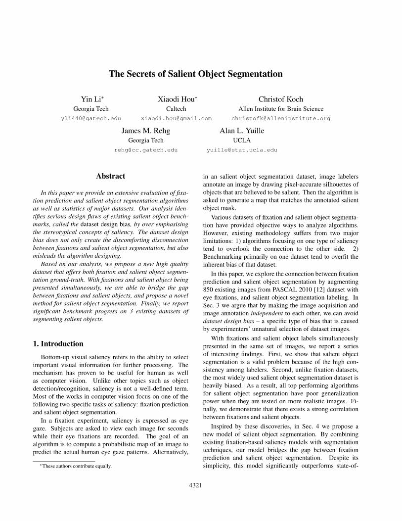
A: Original image B: Full segmentation

C: Fixation ground-truth D: Salient object ground-truth

Figure 1. An illustration of PASCAL-S dataset. Our datasetprovides both eye fixation (Fig. C) and salient object (Fig. D)mask. The labeling of salient objects is based on the full seg-mentation (Fig. B). A notable difference between PASCAL-S andits predecessors is that each image in PASCAL-S is labeled bymultiple labelers without restrictions on the number of salientobjects.

of a saliency map [14, 16, 26]. To make a fair evaluation ofthe algorithm’s true prediction power, Tatler [24] proposeda shuffled-AUC (s-AUC) score to normalize the effect ofcenter-bias. In s-AUC, positive samples are taken from thefixations of the test image, whereas the negative samples arefrom all fixations across all other images.

3. Dataset Analysis

In this paper, we will benchmark on the followingdatasets: Bruce [6], Judd [18], Cerf [8], FT [1], andIS [20]. Among these 5 datasets, Judd and Cerf onlyprovides fixation ground-truth. FT only provides salientobject ground-truth. IS provides both fixations1 as well assalient object masks. While Bruce dataset was originallydesigned for fixation prediction, it was recently augmentedby [5] with 70 subjects under the instruction to label thesingle most salient object in the image. In our comparisonexperiment, we include the following fixation predictionalgorithms: ITTI [17], AIM [6], GBVS [1], DVA [16],SUN [26], SIG [15], AWS [13]; and following salient objectsegmentation algorithms: FT [1], GC [9], SF [23], andPCAS [22]. These algorithms are top-performing ones inmajor benchmarks [4].

1IS provides raw gaze data at every time point. We use the followingthresholds to determine a stable fixation: min fixation duration: 160ms,min saccade speed: 50px/100ms.

3.1. Psychophysical experiments on the PASCAL-Sdataset

Our PASCAL-S dataset is built on the validation setof the PASCAL VOC 2010 [12] segmentation challenge.This subset contains 850 natural images. In the fixationexperiment, 8 subjects were instructed to perform the “free-viewing” task to explore the images. Each image waspresented for 2 seconds, and eye-tracking re-calibration wasperformed on every 25 images. The eye gaze data wassampled using Eyelink 1000 eye-tracker, at 125Hz. In thesalient object segmentation experiment, we first manuallyperform a full segmentation to crop out all objects in the im-age. An example segmentation is shown in Fig. 1.B. Whenwe build the ground-truth of full segmentation, we adhere tothe following rules: 1) we do not intentionally label parts ofthe image (e.g. faces of a person); 2) disconnected regionsof the same object are labeled separately; 3) we use solidregions to approximate hollow objects, such as bike wheels.

We then conduct the experiment of 12 subjects to labelthe salient objects. Given an image, a subject is asked toselect the salient objects by clicking on them. There isno time limitation or constraints on the number of objectsone can choose. Similar to our fixation experiment, theinstruction of labeling salient objects is intentionally keptvague. The final saliency value of each segment is thetotal number of click it receives, divided by the number ofsubjects.

3.2. Evaluating dataset consistency

Quite surprisingly, many of today’s widely used salientobject segmentation datasets do not have any guaranteeon the inter-subject consistency. To compare the levelof agreement among different labelers in our PASCAL-Sdataset and other existing dataset, we randomly select 50%of the subjects as the test subset. Then we benchmark thesaliency maps of this test subset by taking the rest subjectsas the new ground-truth subset. For fixation task, the testsaliency map for each image is obtained by first plotting allthe fixation points from the test subset, and then filter thesaliency map by a 2D Gaussian kernel with σ = 0.05 ofthe image width. For salient object segmentation task, thetest/ground-truth saliency maps are binary maps obtainedby first averaging the individual segmentations from thetest/ground-truth subset, and then threshold with Th =0.52 to generate the binary masks for each subset. Thenwe compute either AUC score or F-measure of the testsubset and use this number to indicate the inter-subjectconsistency.

We notice that the segmentation maps of Bruce datasetare significantly sparser than maps in PASCAL-S or IS.Over 30% of the segmentation maps in Bruce dataset are

2At least half of the subjects within the subset agree on the mask.

4323

completely empty. This is likely a result of the labelingprocess. In Borji et al.’s experiment [5], the labelers areforced to choose only one object for each image. Imageswith two or more equally salient objects are very likely tobecome empty after thresholding. Although Bruce is oneof the very few datasets that offer both fixations and salientobject masks, it is not suitable for our analysis.

For dataset PASCAL-S and IS, we benchmark the F-measure of the test subset segmentation maps by theground-truth subset. The result is shown in Tab. 1.

AUC scoresPASCAL-S Bruce Cerf IS Judd

0.835 0.830 0.903 0.836 0.867

F-measuresPASCAL-S IS

0.972 0.900Table 1. Inter-subject consistency of 2 salient object segmentationdatasets and 5 fixation datasets.

Similar to our consistency analysis of salient objectdataset, we evaluate the consistency of eye fixations amongsubjects (Tab. 1). Even though the notion of “saliency”under a context of complex natural scene is often consideredas ill-defined, we observe highly consistent behaviors a-mong human labelers in both eye-fixation and salient objectsegmentation tasks.

3.3. Benchmarking

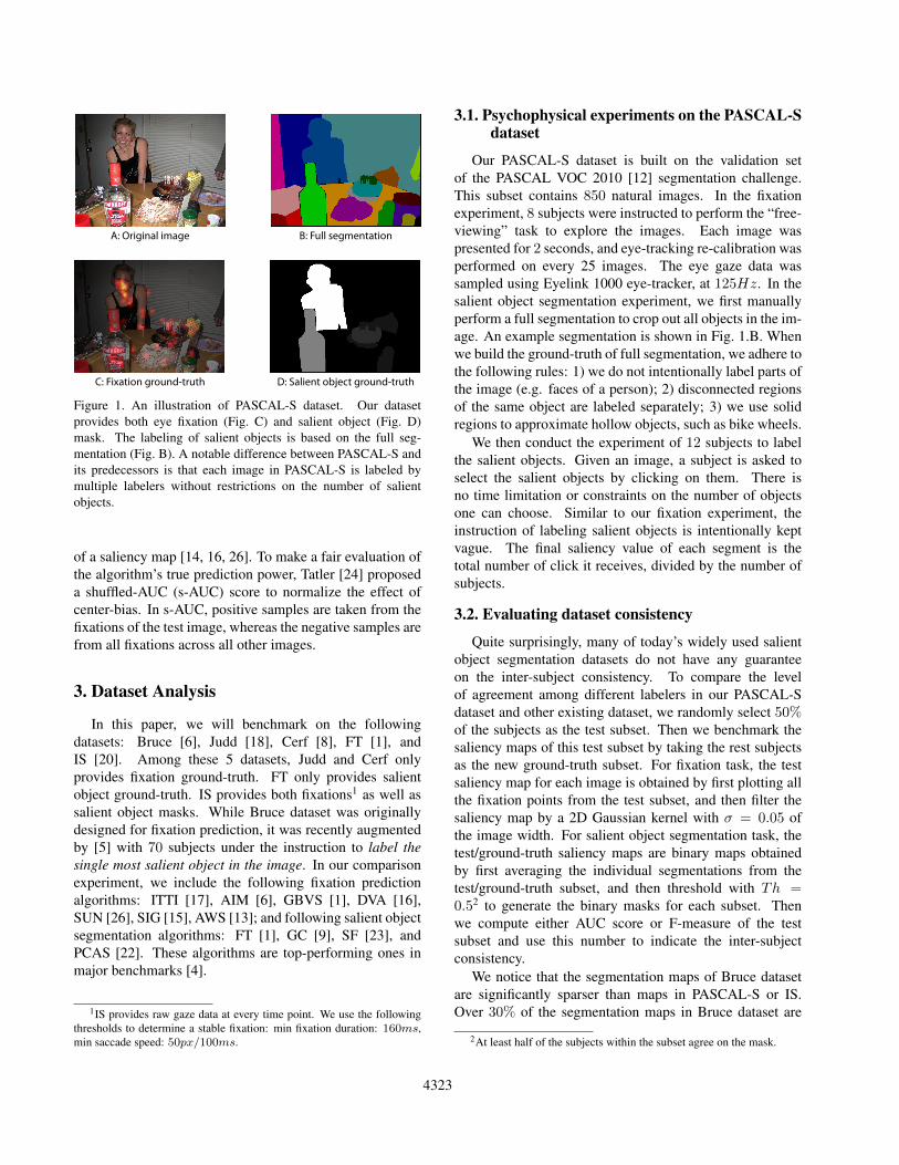
In this section, we benchmark 7 fixations algorithms,AWS [13], AIM [6], SIG [15], DVA [16], GBVS [14],SUN [26], and ITTI [17] on 5 datasets, Bruce [6], Cerf[8], IS [20], Judd [18], and our PASCAL-S. For salientobject segmentation, we bench 4 algorithms SF [23], PCAS[22], GC [9], and FT [1] on 4 datasets, FT [1], IS [20],and our PASCAL-S. For all algorithms, we use the originalimplementations from the authors’ websites. The purposesof this analysis are: 1) to highlight the generalizationpower of algorithms, and 2) to investigate inter-datasetdifference among these independently constructed datasets.The benchmark results are presented in Fig. 2. Sharplycontrasted to the fixation benchmarks, the performance ofall salient object segmentation algorithms drop significantlywhen migrating from the popular FT dataset. The aver-age performance of all 4 algorithms have dropped, fromFT’s 0.8341, to 0.5765 (30.88% drop) on IS, and 0.5530(33.70% drop) on PASCAL-S. This result is alarming,because the magnitude of the performance drop from FTto any dataset by any algorithm, can easily dwarf the 4-year progress of salient object segmentation on the widelyused FT dataset. Moreover, the relative ranking amongalgorithms also changes from one dataset to another.

0 0.2 0.4 0.6 0.8 10

0.05

0.1

0.15

0.2

0.25

Local Color Contrast

0 0.2 0.4 0.6 0.8 10

0.05

0.1

0.15

0.2

0.25

Object Size

FTISPASCAL−S

0 0.2 0.4 0.6 0.8 10

0.03

0.06

0.09

0.12

0.15

Global Color Contrast

0 0.2 0.4 0.6 0.8 10

0.03

0.06

0.09

0.12

0.15

Local gPb Boundary Strengh

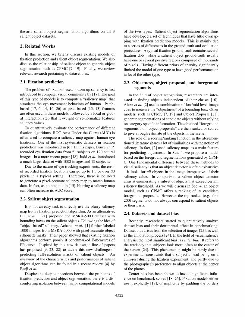
Figure 3. Image statistics of the salient object segmentationdatasets. The statistics of FT dataset is different from otherdatasets in local/global color contrast and boundary strength. Asfor object size, the PASCAL-S contains a balanced mix of largeand small objects.

3.4. Dataset design bias

The performance gap among datasets clearly suggestsnew challenges in salient object segmentation. However, itis more important to pinpoint the cause to the performancedegradation rather than to start benchmark race on anothernew dataset. In this section, we analyze the following imagestatistics in order to find the similarities and differences oftoday’s salient object segmentation datasets:

Local color contrast: Segmentation or boundary detec-tion is an inevitable step in most salient objects detec-tors. It is important to check whether the boundariesare “unnaturally” easy to segment. To estimate thestrength of the boundary, we crop a 5 × 5 imagepatch at the boundary location of each labeled object,and compute RGB color histograms for foregroundand background separately. We then calculate theχ2 distance to measure the distance between two his-tograms. It is worth noting that some of the ground-truth of the IS dataset are not perfectly aligned withobjects boundaries, resulting in an underestimate oflocal contrast magnitude.

Global color contrast: The term “saliency” is also relatedto the global contrast of the foreground and back-ground. Similar to the local color contrast measure, foreach object, we calculate the χ2 distance between itsRGB histogram and the background RGB histogram.

Local gPB boundary strength: While color histogramdistance captures some low-level image features, an

4324

FT IS PASCAL-S

F-Measure

PASCAL-S Bruce Cerf IS Judd0.5

0.6

0.7

0.8

0.9

s-

AU

C

0

0.2

0.4

0.6

0.8

1

AWS AIM SIG DVA

GBVS SUN ITTI Human

SF PCAS GC

FT Human

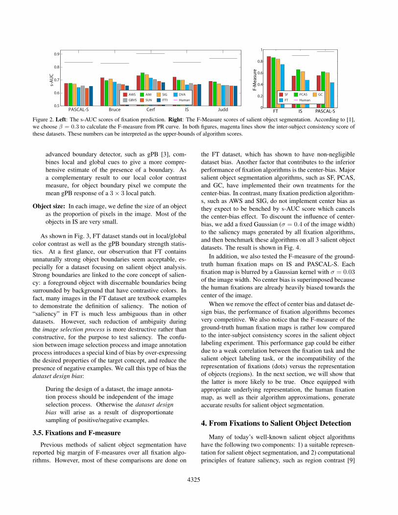
Figure 2. Left: The s-AUC scores of fixation prediction. Right: The F-Measure scores of salient object segmentation. According to [1],we choose β = 0.3 to calculate the F-measure from PR curve. In both figures, magenta lines show the inter-subject consistency score ofthese datasets. These numbers can be interpreted as the upper-bounds of algorithm scores.

advanced boundary detector, such as gPB [3], com-bines local and global cues to give a more compre-hensive estimate of the presence of a boundary. Asa complementary result to our local color contrastmeasure, for object boundary pixel we compute themean gPB response of a 3× 3 local patch.

Object size: In each image, we define the size of an objectas the proportion of pixels in the image. Most of theobjects in IS are very small.

As shown in Fig. 3, FT dataset stands out in local/globalcolor contrast as well as the gPB boundary strength statis-tics. At a first glance, our observation that FT containsunnaturally strong object boundaries seem acceptable, es-pecially for a dataset focusing on salient object analysis.Strong boundaries are linked to the core concept of salien-cy: a foreground object with discernable boundaries beingsurrounded by background that have contrastive colors. Infact, many images in the FT dataset are textbook examplesto demonstrate the definition of saliency. The notion of“saliency” in FT is much less ambiguous than in otherdatasets. However, such reduction of ambiguity duringthe image selection process is more destructive rather thanconstructive, for the purpose to test saliency. The confu-sion between image selection process and image annotationprocess introduces a special kind of bias by over-expressingthe desired properties of the target concept, and reduce thepresence of negative examples. We call this type of bias thedataset design bias:

During the design of a dataset, the image annota-tion process should be independent of the imageselection process. Otherwise the dataset designbias will arise as a result of disproportionatesampling of positive/negative examples.

3.5. Fixations and F-measure

Previous methods of salient object segmentation havereported big margin of F-measures over all fixation algo-rithms. However, most of these comparisons are done on

the FT dataset, which has shown to have non-negligibledataset bias. Another factor that contributes to the inferiorperformance of fixation algorithms is the center-bias. Majorsalient object segmentation algorithms, such as SF, PCAS,and GC, have implemented their own treatments for thecenter-bias. In contrast, many fixation prediction algorithm-s, such as AWS and SIG, do not implement center bias asthey expect to be benched by s-AUC score which cancelsthe center-bias effect. To discount the influence of center-bias, we add a fixed Gaussian (σ = 0.4 of the image width)to the saliency maps generated by all fixation algorithms,and then benchmark these algorithms on all 3 salient objectdatasets. The result is shown in Fig. 4.

In addition, we also tested the F-measure of the ground-truth human fixation maps on IS and PASCAL-S. Eachfixation map is blurred by a Gaussian kernel with σ = 0.03of the image width. No center bias is superimposed becausethe human fixations are already heavily biased towards thecenter of the image.

When we remove the effect of center bias and dataset de-sign bias, the performance of fixation algorithms becomesvery competitive. We also notice that the F-measure of theground-truth human fixation maps is rather low comparedto the inter-subject consistency scores in the salient objectlabeling experiment. This performance gap could be eitherdue to a weak correlation between the fixation task and thesalient object labeling task, or the incompatibility of therepresentation of fixations (dots) versus the representationof objects (regions). In the next section, we will show thatthe latter is more likely to be true. Once equipped withappropriate underlying representation, the human fixationmap, as well as their algorithm approximations, generateaccurate results for salient object segmentation.

4. From Fixations to Salient Object Detection

Many of today’s well-known salient object algorithmshave the following two components: 1) a suitable represen-tation for salient object segmentation, and 2) computationalprinciples of feature saliency, such as region contrast [9]

4325

or element uniqueness [23]. However, none of these twocomponents alone is new to computer vision. On one hand,detecting boundaries of objects has been a highly desiredgoal for segmentation algorithms since the beginning ofcomputer vision On the other hand, defining rules of salien-cy has been studied in fixation analysis for decades. In thissection, we build a salient object segmentation model bycombining existing techniques of segmentation and fixationbased saliency. The core idea is to first generate a set ofobject candidates, and then use the fixation algorithm torank different regions based on their saliency. This simplecombination results in a novel salient object segmentationmethod that outperforms all previous methods by a largemargin.

4.1. Salient object, object proposal and fixations

Our first step is to generate the segmentation of objectcandidates by a generic object proposal method. We useCPMC [7] to obtain the initial segmentations. CPMC isan unsupervised framework to generate and rank plausiblehypotheses of object candidates without category specificknowledge. This method initializes foreground seeds uni-formly over the image and solves a set of min-cut problemswith different parameters. The output is a pool of objectcandidates as overlapping figure-ground segments, togetherwith their “objectness” scores. The goal of CPMC is to pro-duce a over-complete coverage of potential objects, whichcould be further used for tasks such as object recognition.

The representation of CPMC-like object proposal is eas-ily adapted to salient object segmentation. If all salientobjects can be found from the pool of object candidates,we can reduce the problem of salient object detection to amuch easier problem of salient segment ranking. Rankingthe segments also simplifies the post-processing step. Asthe segments already preserve the boundary of the image,no explicit segmentation (e.g. GraphCut [9]) is required toobtain the final binary object mask.

To estimate the saliency of a candidate segment, weutilize the spatial distribution of fixations within the object.It is well known that the density of fixation directly revealsthe saliency of the segment. The non-uniform spatialdistribution of fixations on the object also offers useful cuesto determine the saliency of an object. For example, fixationat the center of a segment will increase its probability ofbeing an object. To keep our frame work simple, we do notconsider class specific or subject specific fixation patternsin our model.

4.2. The model

We use a learning based framework for the segmentselection process. This is achieved by learning a scoringfunction for each object candidate. Given a proposed objectcandidate mask and its fixation map, this function estimates

the overlapping score (intersection over union) of the regionwith respect to the ground-truth, similar to [19].

We extract two types of features: shape features and fix-ation distribution features within the object. The shape fea-tures characterizes the binary mask of the segment, whichincludes major axis length, eccentricity, minor axis length,and the Euler number. For fixation distribution features,we first align the major axis of each object candidate, andthen extract a 4 × 3 histogram of fixations density over thealigned object mask. This histogram captures the spatialdistribution of the fixations within a object. Finally, the33 dimensional feature vector is extracted for each objectmask.

For each dataset, we train a random forest with 30 trees,using a random sampling of 40% of the images. The rest ofimages are used for testing. The results are averaged on a10-fold random split of the training and testing set. We userandom regression forest to predict the saliency score of anobject mask. In the testing phase, each segment is classifiedindependently. We generate the salient object segmentationby averaging the top-K segments at pixel level. We then usesimple thresholding to generate the final object masks. Asour saliency scores are defined over image segments, thissimple strategy leads to fairly good object boundaries.

Note that no appearance feature is used in our method,because our goal is to demonstrate the connection betweenfixation and salient object segmentation. Our algorithm isindependent of the underlying segmentation and fixationprediction algorithms, allowing us to switch between dif-ferent fixation algorithm or even human fixations.

4.3. Limits of the model

Our model contains two separate parts: a segmenter thatproposes regions, and a selector that gives each region asaliency score. In this section we explore the limitationof our model, by replacing each part at a time. First,we quantify the performance upper-bound of the selector,and then, best achievable results of the segmenter is alsopresented.

To test the upper-bound of the selector, we train ourmodel on the ground-truth segments of PASCAL-S (e.g.Fig. 1.B) with human fixation maps. With a perfect seg-menter, this model can accurately estimate the saliency ofsegments using fixation and shape information. On the testset, it achieves a F-Measure of 0.9201 with P = 0.9328and R = 0.7989. This result is a strong validation to ourmotivation, which is to bridge the gap between fixations andsalient objects. It is worth mentioning that this experimentrequires a full segmentation of all objects of the entiredataset. Therefore, PASCAL-S is the only dataset thatallows us to test the selector with an ideal segmenter.

Second, we test the upper-bound performance of CPMCsegmentation algorithm. We match the each segment from

4326

AWSAIM

SIG

DVA GBVS

SUNITTI

AWSAIM

SIG

DVA GBVS

SUNITTI

GCFT

SFPCAS

Salient objectalgorithms

CPMC + �xationalgorithms

Original �xationalgorithms (with �xed center bias mask)

CPMC Best

CPMC Ranking

GT Seg + Human Fixations

CPMC + Human Fixations

Baselinemodels

1

0.8

0.6

0.4

0.2

0

Human Fixations

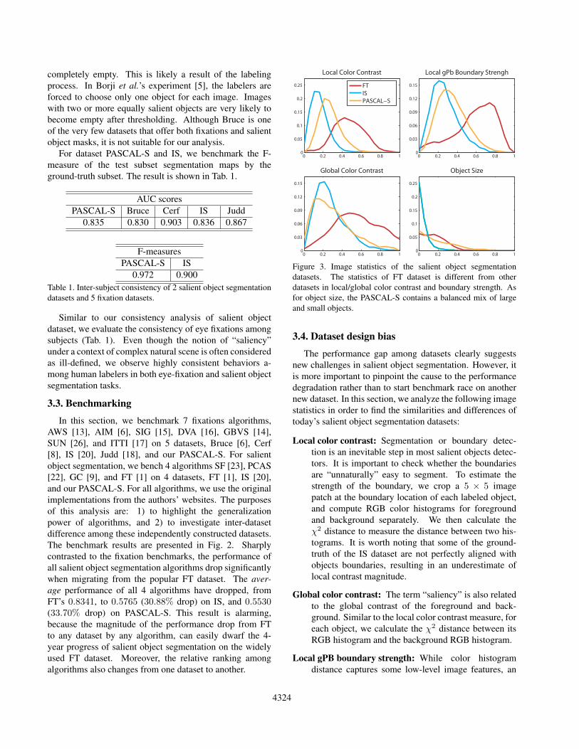
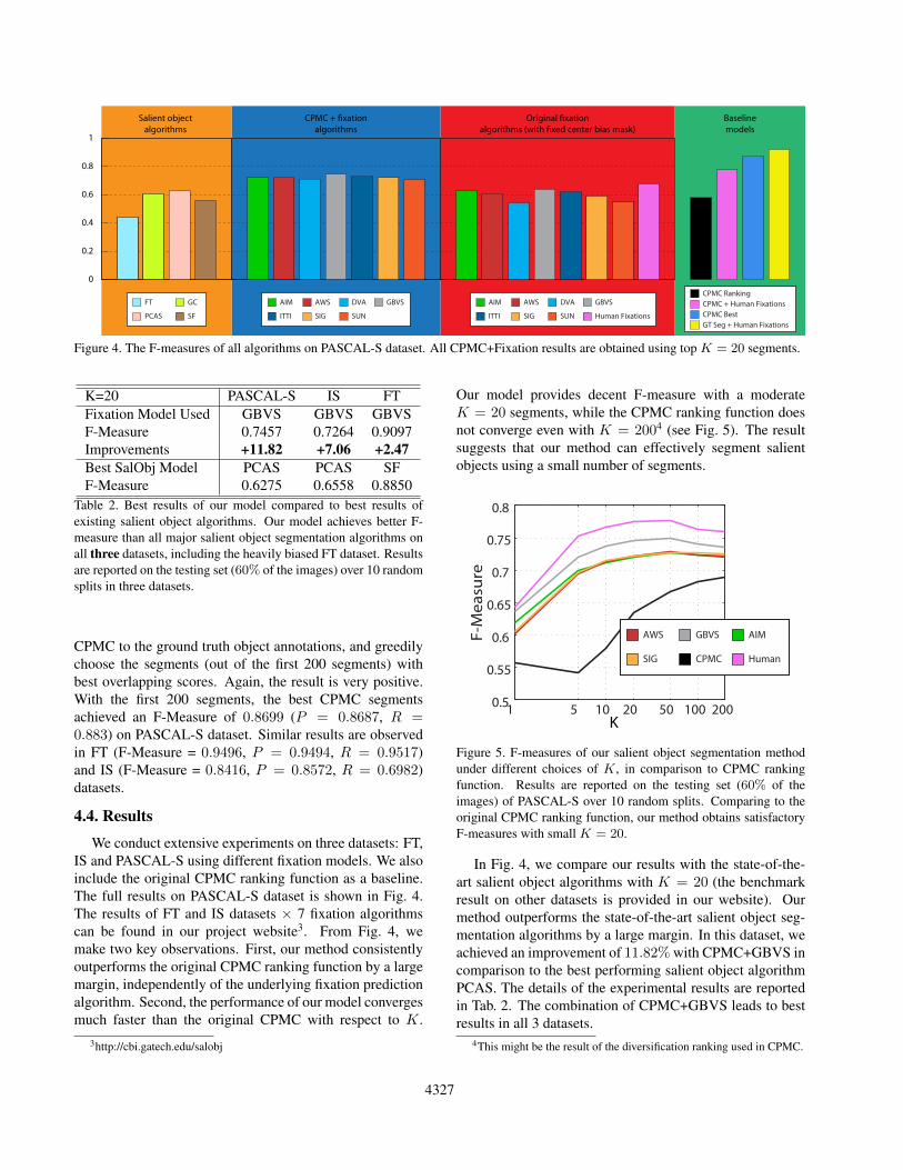
Figure 4. The F-measures of all algorithms on PASCAL-S dataset. All CPMC+Fixation results are obtained using top K = 20 segments.

K=20 PASCAL-S IS FTFixation Model Used GBVS GBVS GBVSF-Measure 0.7457 0.7264 0.9097Improvements +11.82 +7.06 +2.47Best SalObj Model PCAS PCAS SFF-Measure 0.6275 0.6558 0.8850

Table 2. Best results of our model compared to best results ofexisting salient object algorithms. Our model achieves better F-measure than all major salient object segmentation algorithms onall three datasets, including the heavily biased FT dataset. Resultsare reported on the testing set (60% of the images) over 10 randomsplits in three datasets.

CPMC to the ground truth object annotations, and greedilychoose the segments (out of the first 200 segments) withbest overlapping scores. Again, the result is very positive.With the first 200 segments, the best CPMC segmentsachieved an F-Measure of 0.8699 (P = 0.8687, R =0.883) on PASCAL-S dataset. Similar results are observedin FT (F-Measure = 0.9496, P = 0.9494, R = 0.9517)and IS (F-Measure = 0.8416, P = 0.8572, R = 0.6982)datasets.

4.4. Results

We conduct extensive experiments on three datasets: FT,IS and PASCAL-S using different fixation models. We alsoinclude the original CPMC ranking function as a baseline.The full results on PASCAL-S dataset is shown in Fig. 4.The results of FT and IS datasets × 7 fixation algorithmscan be found in our project website3. From Fig. 4, wemake two key observations. First, our method consistentlyoutperforms the original CPMC ranking function by a largemargin, independently of the underlying fixation predictionalgorithm. Second, the performance of our model convergesmuch faster than the original CPMC with respect to K.

3http://cbi.gatech.edu/salobj

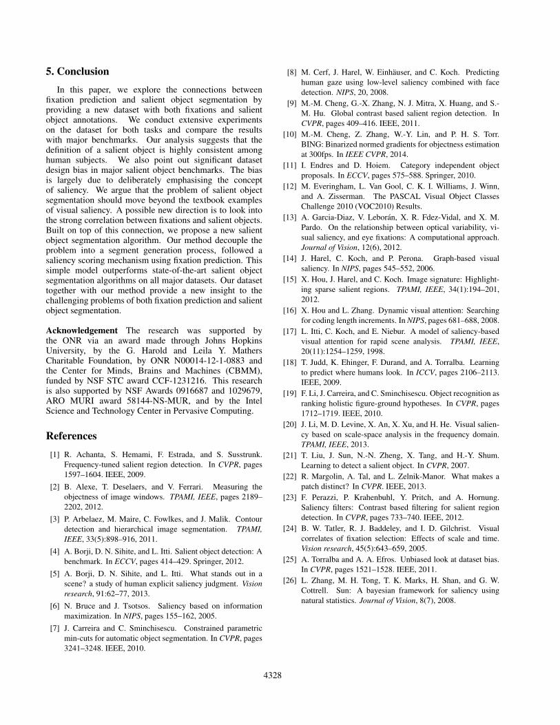
Our model provides decent F-measure with a moderateK = 20 segments, while the CPMC ranking function doesnot converge even with K = 2004 (see Fig. 5). The resultsuggests that our method can effectively segment salientobjects using a small number of segments.

1 5 10 20 50 100 2000.5

0.55

0.6

0.65

0.7

0.75

0.8

F-M

easu

re

K

AWS GBVS AIM

SIG CPMC Human

Figure 5. F-measures of our salient object segmentation methodunder different choices of K, in comparison to CPMC rankingfunction. Results are reported on the testing set (60% of theimages) of PASCAL-S over 10 random splits. Comparing to theoriginal CPMC ranking function, our method obtains satisfactoryF-measures with small K = 20.

In Fig. 4, we compare our results with the state-of-the-art salient object algorithms with K = 20 (the benchmarkresult on other datasets is provided in our website). Ourmethod outperforms the state-of-the-art salient object seg-mentation algorithms by a large margin. In this dataset, weachieved an improvement of 11.82% with CPMC+GBVS incomparison to the best performing salient object algorithmPCAS. The details of the experimental results are reportedin Tab. 2. The combination of CPMC+GBVS leads to bestresults in all 3 datasets.

4This might be the result of the diversification ranking used in CPMC.

4327

5. ConclusionIn this paper, we explore the connections between

fixation prediction and salient object segmentation byproviding a new dataset with both fixations and salientobject annotations. We conduct extensive experimentson the dataset for both tasks and compare the resultswith major benchmarks. Our analysis suggests that thedefinition of a salient object is highly consistent amonghuman subjects. We also point out significant datasetdesign bias in major salient object benchmarks. The biasis largely due to deliberately emphasising the conceptof saliency. We argue that the problem of salient objectsegmentation should move beyond the textbook examplesof visual saliency. A possible new direction is to look intothe strong correlation between fixations and salient objects.Built on top of this connection, we propose a new salientobject segmentation algorithm. Our method decouple theproblem into a segment generation process, followed asaliency scoring mechanism using fixation prediction. Thissimple model outperforms state-of-the-art salient objectsegmentation algorithms on all major datasets. Our datasettogether with our method provide a new insight to thechallenging problems of both fixation prediction and salientobject segmentation.

Acknowledgement The research was supported bythe ONR via an award made through Johns HopkinsUniversity, by the G. Harold and Leila Y. MathersCharitable Foundation, by ONR N00014-12-1-0883 andthe Center for Minds, Brains and Machines (CBMM),funded by NSF STC award CCF-1231216. This researchis also supported by NSF Awards 0916687 and 1029679,ARO MURI award 58144-NS-MUR, and by the IntelScience and Technology Center in Pervasive Computing.

References[1] R. Achanta, S. Hemami, F. Estrada, and S. Susstrunk.

Frequency-tuned salient region detection. In CVPR, pages1597–1604. IEEE, 2009.

[2] B. Alexe, T. Deselaers, and V. Ferrari. Measuring theobjectness of image windows. TPAMI, IEEE, pages 2189–2202, 2012.

[3] P. Arbelaez, M. Maire, C. Fowlkes, and J. Malik. Contourdetection and hierarchical image segmentation. TPAMI,IEEE, 33(5):898–916, 2011.

[4] A. Borji, D. N. Sihite, and L. Itti. Salient object detection: Abenchmark. In ECCV, pages 414–429. Springer, 2012.

[5] A. Borji, D. N. Sihite, and L. Itti. What stands out in ascene? a study of human explicit saliency judgment. Visionresearch, 91:62–77, 2013.

[6] N. Bruce and J. Tsotsos. Saliency based on informationmaximization. In NIPS, pages 155–162, 2005.

[7] J. Carreira and C. Sminchisescu. Constrained parametricmin-cuts for automatic object segmentation. In CVPR, pages3241–3248. IEEE, 2010.

[8] M. Cerf, J. Harel, W. Einhauser, and C. Koch. Predictinghuman gaze using low-level saliency combined with facedetection. NIPS, 20, 2008.

[9] M.-M. Cheng, G.-X. Zhang, N. J. Mitra, X. Huang, and S.-M. Hu. Global contrast based salient region detection. InCVPR, pages 409–416. IEEE, 2011.

[10] M.-M. Cheng, Z. Zhang, W.-Y. Lin, and P. H. S. Torr.BING: Binarized normed gradients for objectness estimationat 300fps. In IEEE CVPR, 2014.

[11] I. Endres and D. Hoiem. Category independent objectproposals. In ECCV, pages 575–588. Springer, 2010.

[12] M. Everingham, L. Van Gool, C. K. I. Williams, J. Winn,and A. Zisserman. The PASCAL Visual Object ClassesChallenge 2010 (VOC2010) Results.

[13] A. Garcia-Diaz, V. Leboran, X. R. Fdez-Vidal, and X. M.Pardo. On the relationship between optical variability, vi-sual saliency, and eye fixations: A computational approach.Journal of Vision, 12(6), 2012.

[14] J. Harel, C. Koch, and P. Perona. Graph-based visualsaliency. In NIPS, pages 545–552, 2006.

[15] X. Hou, J. Harel, and C. Koch. Image signature: Highlight-ing sparse salient regions. TPAMI, IEEE, 34(1):194–201,2012.

[16] X. Hou and L. Zhang. Dynamic visual attention: Searchingfor coding length increments. In NIPS, pages 681–688, 2008.

[17] L. Itti, C. Koch, and E. Niebur. A model of saliency-basedvisual attention for rapid scene analysis. TPAMI, IEEE,20(11):1254–1259, 1998.

[18] T. Judd, K. Ehinger, F. Durand, and A. Torralba. Learningto predict where humans look. In ICCV, pages 2106–2113.IEEE, 2009.

[19] F. Li, J. Carreira, and C. Sminchisescu. Object recognition asranking holistic figure-ground hypotheses. In CVPR, pages1712–1719. IEEE, 2010.

[20] J. Li, M. D. Levine, X. An, X. Xu, and H. He. Visual salien-cy based on scale-space analysis in the frequency domain.TPAMI, IEEE, 2013.

[21] T. Liu, J. Sun, N.-N. Zheng, X. Tang, and H.-Y. Shum.Learning to detect a salient object. In CVPR, 2007.

[22] R. Margolin, A. Tal, and L. Zelnik-Manor. What makes apatch distinct? In CVPR. IEEE, 2013.

[23] F. Perazzi, P. Krahenbuhl, Y. Pritch, and A. Hornung.Saliency filters: Contrast based filtering for salient regiondetection. In CVPR, pages 733–740. IEEE, 2012.

[24] B. W. Tatler, R. J. Baddeley, and I. D. Gilchrist. Visualcorrelates of fixation selection: Effects of scale and time.Vision research, 45(5):643–659, 2005.

[25] A. Torralba and A. A. Efros. Unbiased look at dataset bias.In CVPR, pages 1521–1528. IEEE, 2011.

[26] L. Zhang, M. H. Tong, T. K. Marks, H. Shan, and G. W.Cottrell. Sun: A bayesian framework for saliency usingnatural statistics. Journal of Vision, 8(7), 2008.

4328