the semi-lagrangian method with oblique...

The Semi-Lagrangian method with obliqueinterpolation

M. Mehrenberger

IRMA, University of Strasbourg and TONUS project (INRIA)

Nice, INRIA Project Labs Fratres Meeting, 15-16.10.2015

Joint work including the participation of Yaman Güclü, Guillaume Latu,Maurizio Ottaviani and Eric Sonnendrücker

M. Mehrenberger (UDS) The oblique Semi-Lagrangian method IPL FRATRES, Nice 2015 1 / 31

I. Introduction

Motivation

Exploit alignement of the structures according to the strong externalmagnetic field in plasma turbulence simulations


I. Introduction

Magnetic field

We consider here cylindrical or toroidal geometry

The external strong magnetic field reads B = Bθθ̂ + Bϕϕ̂Here

∇r = r̂ , ∇θ =θ̂

r, ∇ϕ =

ϕ̂

R


I. Introduction

Magnetic field

A general form of the magnetic field in tokamaks is

B = F0∇ϕ+∇Ψ×∇ϕ.

Poloidal flux Ψ for cylindrical or toroidal geometry is supposed to beof the form Ψ = Ψ(r)

⇒ A flux surface is a (θ, ϕ) plane with given r

Trajectories induced by the magnetic field remain in the flux surface.We get

Bθ =−Ψ′(r)

R, Bϕ =

F0

R


I. Introduction

Magnetic field

The pitch angle αpitch is the angle of B with toroidal direction ϕ̂

tan(αpitch) =BθBϕ

=−Ψ′(r)

F0

We define the rotational transform ι

ι =time to do one poloidal rotationtime to do one toroidal rotation

which is the inverse of the safety factor q = 1ι


I. Introduction

Magnetic field

We approximate ι so that it only depends on r (B we call it still ι)

ι(r) =R0

rtan(αpitch) =

R0BθrBϕ

We define the aspect ratio aratio = R0rmax

and have R0r ≥ aratio


I. Introduction

Trajectories in (θ, ϕ) plane

We have∂θrθ′(t) + ∂ϕrϕ′(t) = B(r , θ(t))

and∂θr = r θ̂, ∂ϕr = Rϕ̂

which leads torθ′(t) = Bθ, Rϕ′(t) = Bϕ

andθ′(t)ϕ′(t)

=B · ∇θB · ∇ϕ

=RBθrBϕ

= ι(r)RR0

So, we solve {θ′(t) = ι(r)

ϕ′(t) = R0R = 1

1+(r/R0) cos(θ(t))


I. Introduction

Trajectories in (θ, ϕ) plane

Example that will be used. At rpeak = rmin+rmax2 , we have R0

rpeak' 5.45.


I. Introduction

Specific form of the functions in (θ, ϕ) plane

Initial data is bath of modes g(t = 0) ' sin(mθ + nϕ) subject toadvection like equation, when |B| is dominant

∂tg + v‖B · ∇g ' 0

Gradient along B :

B · ∇g � k‖ cos(mθ + nϕ)

withk‖ = mι+ n R0

R

|k‖| small↔ No much variation of g along B direction.In plasma turbulent simulations, it is observed that

Mode numbers m and n are big (unbounded)k‖ remains small (bounded)


I. Introduction

⇒ Field aligned methods

Many codes simulating turbulence in tokamaks have now a fieldaligned strategyHow to deal with semi-Lagrangian codes (here of interest) ?

Change the grid with curvilinear transform

⇒ First attempt in [Brauenig et al, 2012]

Keep the grid fixed but use field aligned interpolation⇒ General idea developed first in [Hariri-Ottaviani, 2013] (3D fluid code)⇒ First results in Semi-Lagrangian gyrokinetic context together with

curvilinear geometry in the poloidal plane [Kwon et al., 2014]

Field aligned interpolation is a new emerging idea that has startedto be studied and concerns both fluid and kinetic applications,semi-Lagrangian or eulerian methodsAim : reduce the computational size / improve precision


I. Introduction

THE FCI approach

FCI = flux coordinate independantReduce the number of points in ϕ thanks to adhoc transformation(Ottaviani, 2009)

⇒ permits to treat X-point geometry⇒ discretization needs not to be changed

Former transformations : Reduce the number of points in θ (S.Cooley et al., 1991 ; Scott, 2001)

⇒ not able to treat X-point geometry

Here, we do not have to deal with X-point geometry, but still use thesame FCI approach and adapt it to the semi-Lagrangian framework


I. Introduction

Example of FCI approach

Use same fine cartesian grid of the poloidal plane to deal with

Hariri-Ottaviani, CPC (2013) ( c©picture from Hariri talk EFTC2015)


I. Introduction

Our "semi-FCI" approach

Semi-Lagrangian contextUse of polar coordinates (not cartesian)We do not change the discretization in θgeneralization to more complex geometry imply use of curvilineargeometry in the poloidal plane (until last closed surface) ( c©picturefrom Hariri talk EFTC2015)

full FCI also possible (on cartesian grid), but 1D interpolation in θ(see later) would be replaced by 2D interpolation.


I. Introduction

Validation of the approach

Aim of our work : propose one of such an approach and check itsvalidity on different models of increasing difficulty

Description of the method2D advection

⇒ comparison with exact solution

4D screw pinch drift kinetic model in cylindrical geometry

⇒ comparison with known linear instability rate

4D toroidal version of Gysela

⇒ comparison with standard method using different grid resolutions


II. Description of the method

The 2D Semi-Lagrangian method

c©V. Grandgirard slidesM. Mehrenberger (UDS) The oblique Semi-Lagrangian method IPL FRATRES, Nice 2015 15 / 31


Oblique interpolation at feet of the characteristics

⇒ Reconstruction of the needed values through θ interpolation⇒ Reconstruction in the aligned direction

cubic splines not possible in the aligned directionWe use here Lagrange interpolation of odd degreeprevious 1D interpolation is now 2D interpolation



Oblique interpolation at feet of the characteristics

direction given by ι(r)

Use of splitting for (θ, ϕ) advectionFeet through first or second order Taylor expansionDerivative of potential also aligned computed

⇒ Hope to keep Nϕ small ; Nθ (and Nr ) remains big.⇒ Approx 16 points needed per mode


III. 2D advection

2D Translation in ι direction

Advection equation∂tg + B · ∇g = 0

Large aspect ratio limit : R = R0

⇒ Translation parametrized by ιInitial condition g(t = 0) = sin(mθ + nϕ)

L∞ error after one time step ; different time steps are usedDifferent regimes for m = −34 and ι = 1/

√2. Here k‖ = n + mι

n = 5 so k‖ ' −19.04 (old method better)n = 12 so k‖ ' −12.04 (equivalent methods)n = 23 so k‖ ' −1.04 (new method better)n = 30 so k‖ ' 5.96 (new method still better)


III. 2D advection

Error versus Nϕ/n ; Nθ = 200 (or 400 for n = 23)

Lagrange interpolation of degree 9


III. 2D advection

Error versus Nϕ/k‖Lagrange interpolation of degree d

d = 3 d = 5 d = 17

Gain/loss is∣∣∣ n

k‖

∣∣∣M. Mehrenberger (UDS) The oblique Semi-Lagrangian method IPL FRATRES, Nice 2015 20 / 31

IV. Cylindrical geometry

Screw pinch drift kinetic model (in Selalib)

Vlasov type equation for ions

∂t f −∂θφ

rB0∂r f +

∂r Φ

rB0∂θf + v∇‖f −∇‖Φ∂v f = 0, ∇‖ = b · ∇,

External magnetic field B = B0bΦ electric potential satisfies a Poisson type equation

Equations in cylindrical geometry

rmin = 0.1, rmax = 14.5, R0 ' 240that is ρ∗ = 1/14.5 and aspect ratio aratio ' 16.5Nr = 256, Nθ = 512, Nv = 128d = 5 cubic splines in θ and other interpolations.

Different ι

ι = 0 : standard drift kinetic model [Grandgirard et al., JCP, 2006]ι = 0.8



Single mode excitation

Development of Ion Temperature Gradient (ITG) modesDispersion relation gives expected exponential growth rates fromsingle mode excitationIt depends on m and k‖ = (n + mι) bϕ, wherebϕ = 1√

1+(ιr/R)2' 1± 10−3.

We take initial data feq(r , v) (1 + ε(r) cos(mθ + nϕ)), with m = 15

n = 1, for ι = 0⇒ k‖ = 1n = −11 for ι = 0.8⇒ k‖ ' 1

⇒ Results should be the same, at least in the linear phase



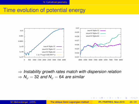
Time evolution of potential energy

⇒ Instability growth rates match with dispersion relation⇒ Nϕ = 32 and Nϕ = 64 are similar



poloidal cut f (T , r , θ,0,0) for T = 4000 (top) andT = 6000 (bottom)

ι = 0,Nϕ = 32 ι = 0.8,Nϕ = 32 ι = 0.8,Nϕ = 64M. Mehrenberger (UDS) The oblique Semi-Lagrangian method IPL FRATRES, Nice 2015 24 / 31


f (T , rmin+rmax2 , θ, ϕ,0) for T = 4000 (top) and T = 6000

(bottom)

ι = 0,Nϕ = 32 ι = 0.8,Nϕ = 32 ι = 0.8,Nϕ = 64


V. Toroidal geometry

GYSELA results

Equations in toroidal geometry

rmin = 4, rmax = 40, R0 = 120That is ρ∗ = 1/40 and aspect ratio aratio = 3Nr = Nθ = 256, Nv = 48d = 5, cubic splines in θ and other interpolations.Bath of modes initialization

Different toroidal discretizations :

Aligned method, with Nϕ = 32Standard method, with Nϕ = 32Standard method, with Nϕ = 64 and Nϕ = 128

shear case : ι(rmin) = 1 ≥ ι(r) ≥ ι(rmax) = 2/3




⇒ 4 times less points for the aligned method for similar accuracy



GYSELA results poloidal (top) and (θ, ϕ) cut (bottom)of electric potential

Nϕ = 32, aligned Nϕ = 32, standard Nϕ = 128, standard


VI. Conclusion

Conclusion/Perspectives

Aligned method is validated on different situations⇒ Oblique interpolation seems to be enough, even for not straight

magnetic field lines (toroidal case)Possible extensions

Improve efficiencyReduce cost of interpolationAdhoc parallelization strategies

Go to larger size machines :ITER : Nr , Nθ ' 4000 Nϕ ' 36000 → Nϕ ' 64 ?

More general geometryworks on curvilinear geometryHexagonal meshdiscontinuous Galerkin method

Add electronscoupling fluid/kinetic ?PIC/semi-Lagrangian ?


VII. Backup


no shear case shear case

⇒ 4 times less points for the aligned method for similar accuracy


VII. Backup

GYSELA results poloidal (top) and (θ, ϕ) cut (bottom)of electric potential

No shear case

Nϕ = 32, aligned Nϕ = 32, standard Nϕ = 128, standard


the semi-lagrangian method with oblique...

Documents