THE SENSITIVITY OF A LINEAR PROGRAM SOLUTION

TO CHANGES IN MATRIX COEFFICIENTS

by

Robert M. Freund

Sloan W. P. No. 1532-84 February 1984

- --- --- --- -- _--.- -��- �.�-�.-..-.-��-I

ABSTRACT

This paper examines the sensitivity of a linear program to changes in

matrix coefficients. Consider the linear program P(e):

maximize z(e) - c x subject to A x b, x> 0,

where Ae F + eG. For all but a finite number of values of for which

the problem is feasible, we show that -I G x where x and ; are anyae

primal and dual solutions to the problem P(e). The theory developed also

includes formulas for all derivatives of z(G), the Taylor series expansion

for z(e) and the Taylor series expansions for the basic solutions to the

primal and dual problems. Furthermore, it is possible to know, by examining

the lexicographic ordering of a certain matrix, whether or not S is one of

the finite possible values of e for which b may not exist, and whether or

not - G x represents a right-sided or left-sided directional derivative of z(e)

at e. f

0749528

_ ___ _.________�___ � �__�____ I__I___I_ CI_ � I_ __

-2-

1. Introduction

The subject of this paper is the sensitivity analysis of a linear program

to changes in matrix coefficients. Whereas the sensitivity of a linear

programming solution to changes in the right-hand side (RHS) and/or objective

row coefficients has been understood for quite some time and is a part of

linear programming practice, such has not been the case for changes in matrix

coefficients. This is due to the apparent complexity of examining the

sensitivity of the inverse of a basis to its original coefficients. This

paper addresses sensitivity analysis of matrix coefficients, and it is shown

that the problem of marginal analysis is simple to solve.

Consider a standard linear program:

max z c x

s.t. Ax = b

x> 0

In some cases, we may want to know how z changes when one coefficient,'say

aij, of A changes to aij + gij, i.e., we seek z(e) and/or z'(e).

In other cases, the problem of changing matrix coefficients arises from

"averaging" constraints of the form, e.g.

kxi

= il ' > 8 which after transformation becomes

E xi + E iil1 i=k+l

__ I ��____�

-3-

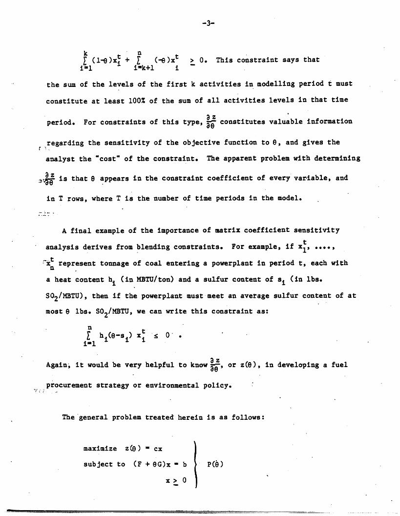
k nE (1-)i + £ (- )xt ,> . This constraint says thatil i-k+l i

the sum of the levels of the first k activities in modelling period t must

constitute at least 100% of the sum of all activities levels in that time

period. For constraints of this type, Az constitutes valuable information

regarding the sensitivity of the objective function to 6, and gives the

analyst the "cost" of the constraint. The apparent problem with determining

ar is that 9 appears in the constraint coefficient of every variable, and

in T rows, where T is the number of time periods in the model.

A final example of the importance of matrix coefficient sensitivity

-,·· ~ ~ ~ ~~~t~~tanalysis derives from blending constraints. For example, if , ....ktn represent tonnage of coal entering a powerplant in period t, each with

a heat content hi (in MBTU/ton) and a sulfur content of si (in lbs.

S02/MBTU), then if the powerplant must meet an average sulfur content of at

most e lbs. S02/MBTU, we can write this constraint as:

i-1

Again; it would be very helpful to know , or z(e), in developing a fuel: -

procurement strategy or environmental policy.

The general problem treated herein is as follows:

maximize z(E) - cx

subject to (F + G)x b P()

x> 0

_I - --- -----------""·------sI*--�I�------·-----�

-4-

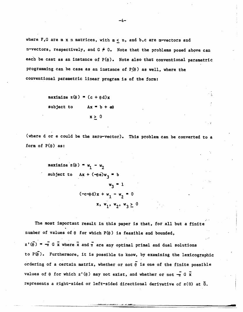
where F,G are m x n matrices, with m < n, and b,c are m-vectors and

n-vectors, respectively, and G 0. Note that the problems posed above can

each be cast as an instance of P(e). Note also that conventional parametric

programming can be case as an instance of Pe) as well, where the

conventional parametric linear program is of the form:

maximize z(e) C (c + d)x

subject to Ax b + ee

x> 0

(where d or e could be the zero-vector). This problem can be converted to a

form of P(e) as:

maximize z(e) - w1 - w2

subject to Ax + (-8e)w 3 b

w3 l 1

(-c-ed)x + w - w2= O

x, wl, w2, w 3 > 0

The most important result in this paper is that, for all but a finite

number of values of e for which P(e) is feasible and bounded,

z'(e) -= G x where x and y are any optimal primal and dual solutions

to P(s). Furthermore, it is possible to know, by examining the lexicographic

ordering of a certain matrix, whether or not e is one of the finite possible

values of for which z'(e) may not exist, and whether or not -m G x

represents a right-sided or left-sided directional derivative of z(G) at .

-- 4L-�-^ �--��-�--�DI-�.�---·�

-5-

The theory developed along the way to proving the above statements also

includes formulas for all derivatives of z(e) at 6, the Taylor series

expansion for z(e), and the Taylor series expansions of the basic solutions

to the primal and dual problems.

Because most large-scale linear programming computer codes furnish x and

r, and can be easily modified to furnish the optimal basis inverse or the

basis L-U decomposition, it should be possible to conveniently generate

z'(e) - -r G x as well as other sensitivity analysis information developedherein

regarding the objective function and the basic optimal solutions to P (G) and its dual.

Section 2 of this paper presents the main results and their proof for the

nondegenerate case. Because degeneracy is prevalent in most large-scale

linear programs, either in fact or due to numerical round-off error, the main

results are also proved for degenerate optimal solutions in Section 3, for

which a deeper analysis of the underlying problem is required.

As regards this paper, my original interest in the problem developed from

the need to compute z'(8) for the sulfur blending constraint described

above, in a particular linear programming application. In the study of this

sensitivity analysis problem, I have tried to follow the standard of George

Dantzig's work-the development of theory in the solution of practical

problems. His standard is one which all can follow.

___l�l�a I ____

-6-

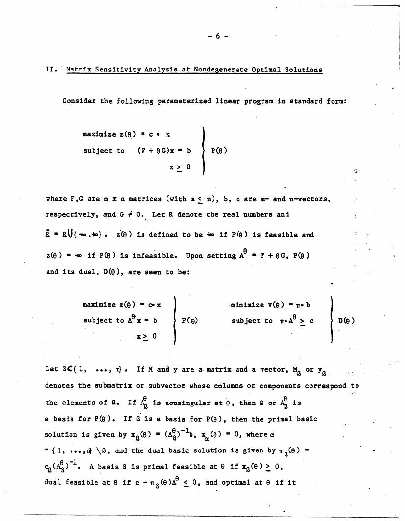
II. Matrix Sensitivity Analysis at Nondegenerate Optimal Solutions

Consider the following parameterized linear program in standard form:

maximize z(e) - c x

subject to (F + G)x = b P(O)

x> 0

where F,G are m x n matrices (with m < n), b, c are m- and n-vectors,

respectively, and G 0. Let R denote the real numbers and r

i - RU{-,Iw}. z() is defined to be i- if P(e) is feasible and

z(e) - A if P() is infeasible. Upon setting A ~ F + OG, P(e)

and its dual, D(), are seen to be:

maximize z(e) = c-x minimize v(Q) = g b

subject to Ax = b P(e) subject to *.Ae > c D(e)

x> 0

Let BC{1, ..., 4. If M and y are a matrix and a vector, Ma or yB

denotes the submatrix or subvector whose columns or components correspond to

e the elements of . If is nonsingular at e, then or A is

a basis for P(e). If is a basis for P(G), then the primal basic

solution is given by x (e) (A@)-lb, xa(e) 0, where a

= {1, ...,* \3, and the dual basic solution is given by w(e) =

c(4)- 1. A basis is primal feasible at e if x(8) > 0,

dual feasible at 9 if c - (G)A < 0, and optimal at 9 if it

__~~~__~~~~~~ ~~__~~_~~~~ ______~~~~~______~~~~_~~~~__~~~~___ * ,i~~~~

-7-

is both primal and dual feasible at . is defined to be a nondegenerate

optimal basis at if (e)Ae - c + x( ) > 0, where x(e) '

(x (e), x ()). This corresponds to both primal and dual

nondegeneracy at the optimal solution.

For a given vector y or matrix M, we define Ilyll maxlyjl and 1111 'j

maxlmijl, the standard supremum norm. An interval I in R is definedi,j

to be any set of the form (a,b), a,b], [a,b), or (a,b], where a,b £ R. The

ith row or jth column of a matrix M is denoted by Mi. or M.j, respectively.

A property ? is said to be true near if there exists > 0 such that ?

is true for all £ (-s, ~E). P is said to be true near - or

near 6+ if there exists > 0 such that? is true for all 8 (8- e ,

or e [, e ), respectively.

If a is a basis for P(8), ()i (det()) a whereby

e -1 P

we see that each component of (A4) is given by ( where p(e) and q(e)

are polynomials in 8 of degree less than or equal to m-l and m, respectively,

and q(8) O. If .G.has only one non-zero row or non-zero column, then p(.)

and q(*) will have degree less than or equal to one, and the problem of analyzing

)-1 through fractional polynomials is tractable, see e.g., Orchard-Hays [2].

Rather than approaching the problem of determining () -1 through fractional

polynomials, we instead derive the Taylor series expansion of (4)1 about

in this analysis. For notational convenience, let B 4 , where is a

-8-

fixed value of and is a given basis for P(8); thus, B is the basis

matrix at e e 9.

Our main result for the nondegenerate case is: ;

THEORM 1: Let B be a (munique) nondegenerate optimal basis for P(i). Let z

and w be the (nique) pr~al and dual optimal solutions to P().

Then for all e near e, B is a nondgenerate optimal basis for

P(e), and

(i) z'(e) -- G x ,

(ii) zk(e) (k:) c(-B GB)k , for k 1, ...., where zk (.) is the kth

derivative of z(.).

.(iii) z (e) C E C(e-e ) (- GB) xGiGO

(iv) zk(e) [ (i) c (-)(i-k)(B 1G)i X8 for k- 1; .

(v) x(e) - (xB(e), (e)) - ( [ ( 8e-)i(--1G%)i ;s,0 ) is the unique optimal

solution to P(8), and

(vi) IT(e) (e > = >i (-G B-i is the unique optimal solution to D(e),i=0

where B = A .

Before proving the theorem, it is important to note why z'(8) -- Gx

on more intuitive grounds. At 8 8, x and T are primal and dual optimal

"" I I I------- I---- I--- I 'III

-9-

solutions to P(e) and D(), and E ' io As x is kept fixed, and changes to

to 0- + A, the new primal system satisfies-:

(F + C + A)G) x b + AG x.

In order to regain the original system of equations, with a right-hand side of

b, b must be changed to b(A) - b - G x. Using the chain rule for differentiation,

, (

z il az

3 bi

Ma - i ; i(-G)iil

- - G x .

This is not a rigorous proof of (i) of Theorem 1 inasmuch as x and Ir are assumed

to remain fixed as 0 varies.

A second perspective on the formula z'(O) - -WGx arises from the formulation

of P() as a Lagrangian problem:

z(C) - ax min. (cx - (Ae x - b)).

If x and r are primal and dual optimal solutions at 8 e $, then

z(O) . max min(cx - ((F + eG)x-b)) - cx - -r Fx - 0nGx + lb.

.. t ..

For small changes in 0, if x and i do not change appreciably, then z' (O) = -TGx.

Again, the proof is not valid because of the assumption of the static nature of

x and as changes near - 0.

_�__L- '--·i-�i -- -P-IIIL 5·1� �i- PT-II .� ._.__�______� �_�

-10-

PROOF OF THEOREM 1:

For all of 8 near 8, exists and so I ) = (B + (8-9)G)( ) I.

-1Premultiplying this system by B and rearranging, we obtain:

-1 -l -1c, 1sB1 -_ (o - ) (B G (A)

By recursively substituting for ( )-1 in this last expression, we obtain:

This series converges for all 18-91 < - (i-B GI) . The series in

(v) follows from the fact that xB(8) (A)-b. (iii) follows from the

equation z(8e) cBxB(8), and (i), (ii), and (iv) derive from (iii).

,eC - CA~- - Z ) Cei CjB'G - 80 Ce)' c C-G B i -i-O B i-o B

i(e-9) f -GB ) , which is the series in (vi). Because B is a nondegenerate

i.O

basis for P(e), (8)A? - c + x(o) > 0, and so for all near 8,

s(0)A - c + x(8) > 0 as well, thereby showing that x(O) and r(8e) are feasible

and nondegenerate solutions to P(e) and D(8).

Because most large-scale linear programming computer codes compute and

record the primal and dual solutions and the basis inverse or the L-U

decomposition of the basis, each of the terms of the series in (i)-(vi) can

readily be computed. Regarding the higher-order terms of these series, the

computational burden of computing these terms is probably excessive, unless

_���___

-·------· ·---�-------- ·�-----�p� �����

-11-

B-1G is very sparse. (Even when G is sparse, as it may possibly be in

any particular application, B- G may not be sparse.)

From a theoretical point of view, the nondegeneracy hypothesis of Theorem

1 is satisfied for P) except for a certain collection of problem data

(b,c) which has measure zero. However, as a matter of experience, most

large-scale linear programs exhibit substantial degeneracy in the optimal

basis, either in fact (primarily the result of special structures) or due to

numerical roundoff. It thus is necessary to examine the general (degenerate

or nondegenerate) case of P) if the formulas of Theorem 1 are to have

practical significance.

___·l___l__s___lls___I___�_II___IC____

III. Matrix Sensitivity Analysis at Degenerate or Nondegenerate Solutions

Let {i P( ) is feasible and bounde , i.e., is the set of

for which -~ < z(8) < + . The main result of this section is:

THEOREM 2: Let B be an optimal basis for P(9). Let and w be the primal

and dual basic optimal solutions to P(j) corresponding to B.

Then, except for a finite number of values of e e e , equations

(i) - (vi) of Theorem 1 are true for all e near 0.

The proof of this theorem follows from the following lemma.

Lema 1: (i) {Iz( ) ( )} is a finite union of intervals.

(ii) {eIB is an optimal basis for P(e)) is a finite union of

intervals for each BC{1,...,n}.

(iii) {(1 -a < z(e) +)- is a finite nion of intervals.

(iv) {e z() ' -} is a finite union of intervals.-

PROOF: For any given value of 8, we can assume that A has full rank, by

appropriate addition of artificial variables, if necessary. Thus, if

z(e) i= for some 8, there exists a basis such that xB(8) > 0, and a

column j such that (A)-lAj 0 and cj - fwB(e)A > 0. Therefore,

{e z(e) " A-,.} U fJ { det(A- 0) ' c(AO) -b . 0{

{I(A0) A < °} n{Cj c} (A() A. 0 > O}. Because det(A0 ) is a polynomial{e 1 e, - c.e A Ain (of degree at most m), ({1 detfAh) # 01 is a finite union of intervals.

We can assume that if det (A) ' 0, then -det (A) > O, by rearranging columns,

if necessary, whereby { I| (A-l) b 2 0} = {O adj(A )b > 0, and each

constraint of this latter formulation is a polynomial. Hence the set

-13-

is the intersection of a finite union of intervals, which is a finite union of

intervals. Similarly, (CA A } - {Aladj() < O} lad) < O}, each constraint of

of which is a polynomial ine, and thus this set also is a finite union of

intervals. Finally {(6 c-c(A) Ad > O) ({l (det(A ))cj > c (adj( A)A )} which

is also a finite union of intervals. Thus {elz(e) - WI) is the union over all

of the intersection of a finite union of intervals, which is itself a finite

union of intervals. This proves (i). To prove (ii), note that {(13 is anj.: '

optimal basis for P(e)} - {(1 det(A) # O, (A)-b > and

c(13 ) 1A> c - {81 det(o) a O} {9(1 adj()b > 0} (n i(adj(s he

c(det(A)}. Using the logic employed above, the latter formulation is the

intersection of three sets, each of which is a finite union of intervals.

(iii) follows from (ii) and the fact that there are a finite number of bases,

and (iv) follows from (i) and (iii). 0

Let I () I {e1 is an optimal basis for P(e)}, and let B be the

union over all c {1,...,n} of the set of endpoints of the intervals of

3 (1). 7 then is the set of "breakpoints" of the function z(O), i.e., is

the set of points at which a basis changes to primal or dual infeasible from

feasible, or the basis matrix becomes singular.

Proof of Theorem 2: For any e'Vg\ , and any optimal basis for P(8), there is an

,open interval (8- , ef) such that is an optimal basis for P(e) for all

___II�:_� -�� -�------^---------------

-14-

e8 (-e 4). This being the case, the power series' of (i)-(vi) of

Theorem 1 converge. SinceX is a finite union (overall 3 C {l,...,n}) of a

finite number of endpoints, B is finite, proving the theorem. a

We now turn our attention to the task of determining for a given problem

P(e) if e is a breakpoint, i.e., an element of . If P(9) has a non-

degenerate solution, then e is not an element of 8, and so the conclusions'of

Theorem 1 hold true. However, even if P(e) exhibits a degenerate optimal basic

solution, e need not be an element of . - This is illustrated in the following

example, where the initial tableau is shown, followed by Tableaus 1-4, which

illustrate four different bases and basic solutions. In these tableaus, the

basement row represents the objective function z(e).

____� __��1�1� 1__ � P1_II� �Ds I(···llili·L�·li·�-·�·111�······�·-11� I�-�l�L- ·li-----· ·-·-�I -�I

i

-15-

Initial Tableau

RHS xl x2 x3 x4

1 1-e 0 2 59

1 0 1-8 -1- 1

Q0 1 1 1 -4

Basis Range of Optimality

, Tableau 1, -i

x, .:.RHS Xt x2 x3 x4

2 581-e 11

0 1 -1-81-8

X1 - {1,2} -5 < < 1

1w--

-2 -5f1- 1-

Tableau 2'

RHS x x2 .x3 X4

21' 514 2

. T 1 -2

2 -5-280 0 0- -

Tableau 3

RHS x1 x2 X3 x4

-1 8-1 1 -1

3 2 5 O 32+5e+22 1 e -192

1- O O

z 2 = {2,3}

B3- {1,3}

-3 < < 1

-5 < e <-3_ _ ,

1

11e

1= ij[~~~~~~~~~~~~~~~~~~~~~~~~~~~~~~~~~~~~~~~~

�-�11�1�-�--- -- �'�--�-I---�-�`- ���--�II�-���----~~�`""~����-`-�-I�-I��� �. .. ,. , <- .

-16-

Tableau 4

RHS x1 x2 X3 x4

1-5e 2 +5e+21 -5o +

1 0 1- -1- 1

.. 3-e 5 .. - el- )(54e )0

i , , , , , ,, .' '

4 = 1,4} < -5

This exmple has degenerate optimal solutions for -5 < e < 1, yet the

only breakpoints areZ - {-5,-3,1}. For -5 < 8 < 1, there are multiple

optimal solutions to the primal. X1 is optimal over the range

-5 < e < 1, yet the ranges of optimality for 2 and 3 are [-3,1) and

[-5,-3], respectively. As e decreases below -5, B1 and 3 lose

feasibility, and 4 is the only optimal basis in the range (-w,-5].

We now show how to determine if 9 is a breakpoint or not (without

pivoting beyond the final tableau) given the problem data (F,G,b,c) and an

optimal basis for P(e). In order to demonstrate how this can be done,

some more notation and a result from linear algebra are first presented.

Let fP(8) and f'(8) denote the directional derivative of f() in the plus

and minus direction, i.e., f () = lim :,+h) - re) ) lim ( -f (e+hLet a denote the h

Let denote the lexicographic ordering for vectors and extended to matrices,

see e.g. Dantzig [1], where M 0 if HMi. 0 for each row i of M. Given a

vector y, define M 0 mod y if Mi 0 whenever Yi O, and M 0 mod y

if Mi. (0,...,0) whenever Yi 0. The orderingn mod y corresponds to

the lexicographic ordering when y 0, otherwise it corresponds to the

x� �

-17-

lexicographic ordering restricted only to those rows of M for which the

corresponding components of y are zero. The following intermediate results

will be used in the analysis:

Lemma 2: (See Veinott [31) If D is a matrix of rank r, then there is a

j < r such that MD v, MD 2v, MD3, ... , are all linear

cbinations of MD v.0. IID

One version of this lemma is presented in [3].. It is proved here for

completeness.

iPROOF: The vectors D v, il, ... all lie in the subspace L spanned by the

columns of D. Thus, the vectors Dv, ..., D+ v cannot all be linearly

independent, whereby there exists j < r such that D+lv is a linear

combination of D v., D. We now show by induction that Div is a

linear combination of Dv, ... , DJv for all i-l,.... Clearly, this is

true for i-l, ... , j+l. Suppose it is true for k > j+l. Then

D X9i, &v, and Dk+lv - E Dv. But since Dj+l is a linear

combination of D v, .... , DJv, the result follows afterpremultiplication by M. 0

Lena 3: For given matrices , D and a vector v, let-y(e) - E lDiv for all{~+ : '- · l ,i o

near 0, and suppose y(O) Mv > 0. Define Q and pk to be the

k-column matrices Q = [MD v, ... , MDkvI andk 1 kk = [M(-D) v, ..., M(-D)kv] fdr k = 1,.... Let

r be the rank of D.

-·IILu-·llllllp·llll·II·-- �CII --- II

Then:

(i) y(c) > 0 for all c near + if and only if Qr 0 od y (0),

(ii) y(e) > 0 for all c near 0- if and only if pr 2 0 od y(0),

(iii) y(E) > 0 for all c near O if and only if Q r 0 rod y(O) and

p O nmod y(O).

PROOF:

Because y(O) > O, Y(e) > 0 for all near 0+ if and only if the

infinite matrix Qo has a lexicographically nonnegative row i whenever

Y() i 0 , i.e., whenever 0 mod y(O). However, in view of Lemma 2,

Q * O0 mod y(O) if and only if Qr 0 nmod y(O). This shows (i). (ii)

follows from a parallel argument and (iii) follows from (i) and

(ii). o

We are now ready to examine the question of whether or not e is a

breakpoint. For a given problem P(9) with an optimal basis , let x and i

denote the optimal primal and dual basic solutions for . Define the following

mxk and nxk matrices, for kl,...:

-k 2 _B -1 G) 1 B--. 2-X (-BG x13 (-B ) x ... , (-B ) x ],

yk [(B-lG)l s' (B 1G) 22 , (B 1G)k XB

[C- (C-B ), (-GAB 1) -G Al , and

Dk-- [i(G 8B-1)A, (GB-1 )2A, ... , ;i(G B-l)kA]

TBEOREI 3: Let B be an optimal basis for P(8). Let x, i, Im, and m be

defined as above. Then:

(i) 0 is ot a breakpoint if and only if i } 0 mod 1B and

Em B mnod (AC), k -ooAd (;A-c), yk r O mod i, and k O mod (A-c).

(ii) If ~0 mod "B and 0 nod (-c), then B is an optimal

-19-

basis for P(e) for 8 near 8, and equations (i)-(vi) of

Theorem 1 hold true for all 9 near , with zk(. ) replaced

kby z+(.).

(iii) If 0s nod xl and i O od (A-), then is an

optimal basis for P(C) for near , and equations (i)-(vi)

of Theores 1 hold true for all near e , with z. (-) replaced

by zk(. ).

Proof: we first prove (ii). Suppose i' 0 d ;2 and .O od (A-c).

mo

Let - , D - (-B1G), and - fg. Not tat xs(e) - s0(eS )%i, nd *o

by le a 3, x(e) > O for all e r if and oly if Q O nod . However,

,1 Xrr and Prb o od if and onl if i¶ O mod sz, since r < Th. tusBm i s

primal feasible for all e near e if and only if p 0 od B. As regards the

the dual, let M- A, D - ( BB),and v - . Note that

i0a(9)A-c (G )i(Oi)t, and so by T- 3, sg(O)A-c > O for, all a

if and only if Qr 0 mod(rA-c). The latter is true if and only if

a' 0 mod (A-c). Thus is dual feasible for all near +, and so is

optimal for P() for all 8 near , whereby equations (i)-(vi) of Theore 1

hold true, with z ( ) replaced by z+(-).

� -Illllaa�aa�nar�·l---------_________�

V - ..1

-20-

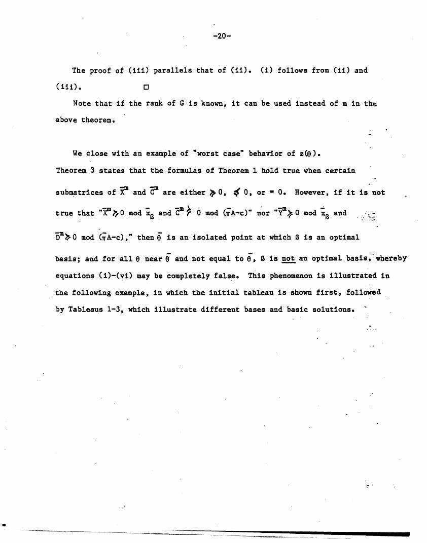
The proof of (iii) parallels that of (ii). (i) follows from (ii) and

(iii) .

Note that if the rank of G is known, it can be used instead of m in the

above theorem.

We close with an example of "worst case" behavior of z(O).

Theorem 3 states that the formulas of Theorem 1 hold true when certain

submatrices of 3m and Cm are either * 0, %4 0, or 0. However, if it is not

true that "xm~30 mod x and m 0 mod G(A-c)" nor Ymr O mod and

D mbO mod (A-c)," then is an isolated point at which is an optimal

basis; and for all near e and not equal to e, B is not an optimal basis, whereby

equations (i)-(vi) may be completely false. This phenomenon is illustrated in

the following example, in which the initial tableau is shown first, followed

by Tableaus 1-3, which illustrate different bases and basic solutions. v

-� 111`�~�"�--------------

-21-

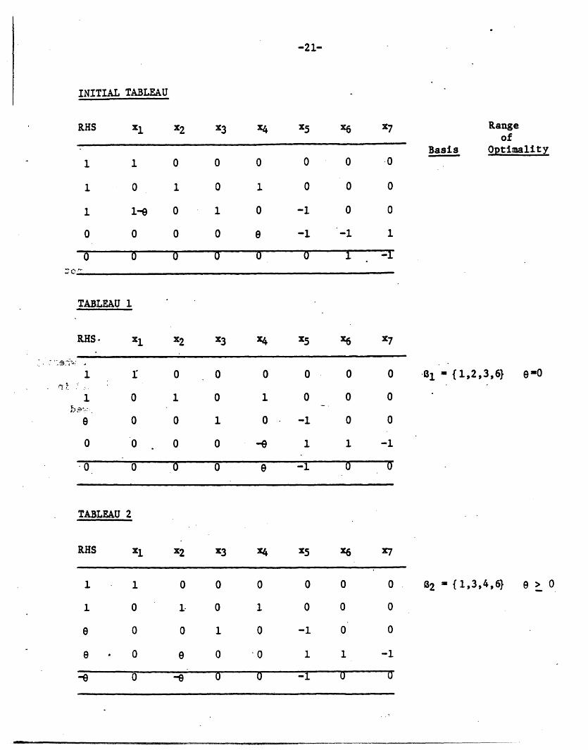
INITIAL TABLEAU

Xi x2 X3 X4 x5 X6 X7

Basis

Rangeof

Optimality1 1 0 0 0 0 0 .0

1 0 1 0 1 0 0 0

1 1-8 0 1 0 -1 0 0

O 0 0O 0 -1 -1 1

0 0 a ° O0 1 -- 1

TABLEAU 1

RHS. X1 x2 X3 X4 x5 x6 x7

. .~~~~~~~~~~~~~~~~~~~~~~

r 0 0

o 1 0

o o 1

o0 0 0

o o o

o 0 0 0

1 o 0 0

O0 -1 0 0

-e

e

·B1 ' {1,2,3,6}

1 1 -1

-1 0 0

TABLEAU 2

RHS x1 X2 x3 x4 x5 X6 x7

O O 0 0 0

1. 0 1 0 0

0 1 0 -1 0

e 0 0 1 1

O- O -1 U

0

0

0

-1

o

B2 { 1,3,4,6}

RHS

7

1

1

0

eo-

1

1

-8

1

0

0

0

6'

e > 0

III

---~~~~~~~~~~~~---" II -------~~~~~~~~~~~~~~~~~~~~~~~~~~~~-- -----

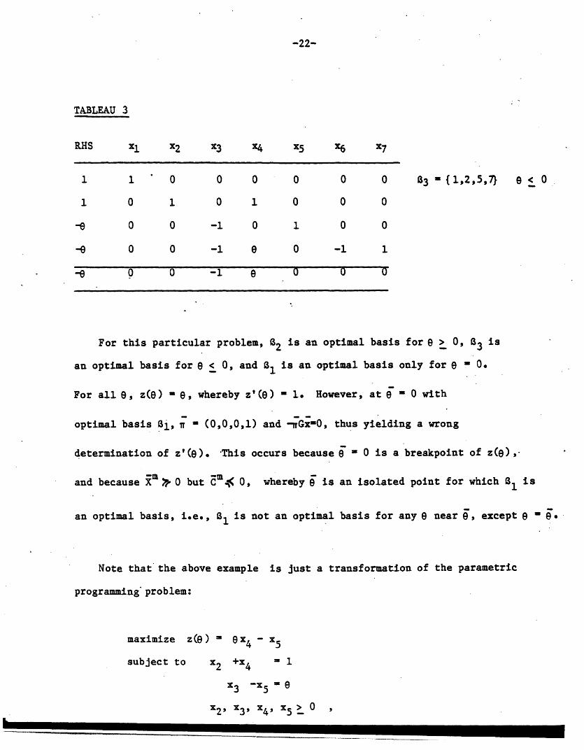
TABLEAU 3

RHS xl x2 X3 X4 X5 x6 x7

1 1 0 0 0 0 0 0

1 0 1 0 1 0 0 0

-e 0 0 -1 0 1 0 0

-e 0 0 -1 e 0 -1 1

-e 0 0 -1 -e O O '

3 - {1,2,5,7 < 0

For this particular problem, 2 is an optimal basis for e > O, 3 is

an optimal basis for 8 < 0, and 1 is an optimal basis only for e - 0.

For all 8, z(O) - 8, whereby z'(e) - 1. However, at 98 0 with

optimal basis i, - (0,0,0,1) and -GrGxO, thus yielding a wrong

determination of z'(e). This occurs because = O is a breakpoint of z(9),

and because m 0 but m,( 0, whereby is an isolated point for which B1 is

an optimal basis, i.e., B1 is not an optimal basis for any near , except 9 ' 0.

Note that the above example is just a transformation of the parametric

programming problem:

maximize z(e) - x 4 - x5

subject to x2 +x4 = 1

X3 -x 5 = e

x2, 3, x4, X 5 > 0

------ - - ----

-23-

which shows that even this seemingly well-behaved parametric programming

problem can have a badly behaved breakpoint.

43 > e

I- -- ~~ - - - -- ~ ----------- --

ACKNOWLEDGEMENTS

I have had numerous discussions regarding matrix coefficient sensitiyity

analysis with Professor James Orlin. This interaction has been invaluable

toward the development of this paper.

--- ---

-25-

REFERENCES

[1] Dantzig, George B., Linear Programming and Extensions, PrincetonUniversity Press, Princeton, N.J., 1963.

f[ 2] Orchard-Hayes, William, Advanced Linear-Programming Computing Techniques,McGraw-Hill, New York, 1968.

si[3] Veinott, A.F., "Markov Decision Chains", in Studies in Optimization,

vol.10, G.B. Dantzig and B.C. Eaves (eds.), The MathematicalAssociation of America, 1974.

��__________11__1____l_�l__�_� __�_�II_ _ ���11 1��_11�