the “smart money” effect: retail versus institutional

1

The “Smart Money” Effect: Retail versus Institutional Mutual Funds

Galla Salganik∗

Ben-Gurion University of the Negev, Guilford Glazer Faculty of Business and Management

This version: December 5, 2011

ABSTRACT

Do sophisticated investors exhibit a stronger “smart money” effect than unsophisticated ones? In this

paper, I examine whether fund selection ability of institutional mutual fund investors is better than

that of retail mutual fund investors. In line with the studies of Gruber (1996), Zheng (1999), and

Keswani and Stolin (2008), I find a smart money effect for investors of both institutional and retail

mutual funds. Surprisingly, the results suggest that investors of institutional funds, with a higher

representation of more sophisticated investors, do not demonstrate a better fund selection ability.

JEL: G19, G23

Keywords: smart money effect, mutual funds, institutional investors, retail investors, institutional funds, retail funds, investment decisions

∗

Department of Business Administration, Guilford Glazer Faculty of Business and Management, Ben-Gurion University

of the Negev, P.O.Box 653, 84105 Beer Sheva, Israel. E-mail: [email protected]. Phone: +972 8 642 87 08. I

would like to thank Jenke ter Horst, Paul Sengmueller, Luc Renneboog, Frans de Roon, Shmuel Hauser, Joost Driessen,

Peter de Goeij, and seminar participants at Ben Gurion University of the Negev for valuable comments and suggestions.

All remaining errors and omissions are mine.

2

1 Introduction

More than a decade ago, Martin Gruber (1996) in his paper “Another Puzzle: The Growth in

actively Managed Mutual Funds” attempted to find a reasonable explanation for the question why

the industry of actively managed mutual funds has grown so fast. The main finding of Gruber was

that investors in actively managed mutual funds have fund selection ability allowing them to detect

future best-performing funds. Gruber defines conditions required for the “smart money”

phenomenon to exist. These conditions are superior fund manager abilities and superior ability of

sophisticated investors to detect talented managers. Addressing the question why there are still

consistently poorly performing funds, Gruber notes that these funds remain due to the presence of

“disadvantaged” investors. According to the author, the disadvantaged investor group includes

unsophisticated individuals, restricted accounts of institutional investors such as pension funds, and

tax disadvantaged investors whose capital gain taxes make divestment of money from a fund

inefficient. Gruber’s study initiated the whole stream of literature investigating whether mutual fund

investors are smart ex ante moving to the funds that will perform better – the “smart money” effect

(see, for example, Zheng (1999), Sapp and Tiwari (2004), Keswani and Stolin (2008)).

Nowadays, the number of actively managed funds has continued to grow. Moreover, since

the early 1990s, a new class of so-called institutional funds has emerged (James and Karceski

(2006)). Instead of focusing on traditional mutual funds’ investors – regular individuals, those funds

serve exclusively institutional investors such as corporations, non-profit organizations, endowments,

foundations, municipalities, pension funds, and other large investors, including wealthy individuals.

Thereby, mutual funds were virtually divided into retail and institutional according to their clientele

focus. Thus, following Gruber’s terminology, clienteles of retail funds, which focus primarily on

individual investors, can be classified as an unsophisticated type of disadvantaged investor

(Alexander, Jones and Nigro (1998), Del Guercio and Tkac (2002), Palmiter and Taha (2008)), while

clienteles of institutional funds either fall into the category of sophisticated investors or into the

group of disadvantaged investors of account restriction or tax issue type.

In the context of the “smart money” effect in mutual fund industry, investor composition

determines the growth rate of actively managed funds. Following Gruber’s line of reasoning, retail

and institutional funds, which have different – in terms of Gruber’s (1996) investor classification

into “sophisticated” and “disadvantaged” types – investor compositions, should grow at a different

3

pace. In fact, the number of institutional funds has increased disproportionally faster (James and

Karceski (2006)). Thus, the question to ask is whether Gruber’s smart money effect can also explain

the difference in the growth rate of retail and institutional funds, and in particular whether investors

of these two types of funds indeed demonstrate dissimilar fund selection abilities.

In this paper I reexamine the smart money effect comparing the fund selection abilities of

investors of retail funds, (representing mostly unsophisticated individual investors) against this

ability of investors of institutional funds, among whom – though a higher proportion represents

sophisticated investors – are also disadvantaged investors, due to account restriction or tax issues.

I explore this question by examining the smart money effect separately for investors of retail

and institutional funds. I use the complete universe of diversified U.S. equity mutual funds for the

period January 1999 to May 2009 in the CRSP Survivor-Bias Free U.S. Mutual Fund Database. I use

CRSP’s classification of institutional and retail funds to identify fund types. Note that this

classification may not be a precise identifier of investor type. For instance, the final investment

decision of 401k plans’ participants is taken by an individual investor, while their capital flows may

combine flows of either an institutional or a retail fund. Nevertheless, it seems reasonable to assume

that the classification of funds into retail and institutional implies differences in investor composition

of the two types of fund. In particular, the overwhelming majority of retail fund investors apparently

are regular individuals. At the same time, institutional investors, if participating in mutual funds, can

be expected to invest in institutional funds. Furthermore, presumably more sophisticated institutional

investors influence flows of institutional funds, while flows of retail funds are determined by

investment decisions of unsophisticated – individual investors.

Following Gruber (1996), Zheng (1999), Sapp and Tiwari (2004), and Keswani and Stolin

(2008), at the beginning of each month and for each type of fund, I construct two portfolios of new-

money. The first portfolio consists of all funds with a positive net cash flow realized during the

previous month. The second portfolio comprises all funds with a negative net cash flow realized over

the same month. Next, I estimate the performance of each of the portfolios in the subsequent month

using both the Fama-French’s (1993) model and the Carhart’s (1997) model including a momentum

factor.

To test for fund selection ability on the part of investors of each fund type, I examine the

difference between the alphas of the positive and negative cash flow portfolios of the corresponding

4

fund sample. Thus, to compare money smartness of investors of retail and institutional funds, I

compare the estimated differences.

In line with the studies of Gruber (1996), Zheng (1999), and Keswani and Stolin (2008), I

find a smart money effect for investors of both institutional and retail mutual funds. The effect is

robust to different measures of performance and flows, and controlling for stock return momentum

and investment style. Consistent with the findings of Zheng (1999), I find that the smart money

effect comes mainly from small funds. I also observe that investors of both types of funds

demonstrate better fund selection ability over expansion periods than during recession periods.

Surprisingly, the results suggest that investors of institutional funds, with a higher


Probably, performance persistence, widely documented by existing mutual fund literature (Sharp

(1966), Grinblatt and Titman (1989a, 1992), Hendricks, Patel and Zeckhauser (1993), Gruber

(1996), Elton, Gruber and Blake (1996), Bollen and Busse (2002), Wermers (2003), Kosowski,

Timmermann, Wermers and White (2006)), represents one of the main observable attributes of the

superior ability of the fund manager, while past return information is accessible and widely used by

both types of investors (Alexander, Jones and Nigro (1998), Del Guercio and Tkac (2002), Palmiter

and Taha (2008)). If so, a higher level of financial sophistication does not necessarily lead to better

fund selection ability. Alternatively, performance persistence, providing some extent of return

predictability, together with accessibility of past return records and financial advisers’ services,

allows unsophisticated investors to demonstrate fund selection ability as well.

Concurrently, the results indicate dissimilarities in the cash flow development for retail and

institutional funds. The observed dissimilarities can be a result of difference in investment decision

patterns characterizing investors of each fund type (Nofsinger and Sias (1999), Grinblatt and

Keloharju (2001), Del Guercio and Tkac (2002), Froot and Teo (2004), Sias (2004), Gallo, Phengpis

and Swanson (2008)), and deserve further investigation.

The remainder of this paper is organized as follows. Section 2 provides an overview of

relevant literature. Section 3 discusses the mutual fund data sample and the methods used to measure

cash flows and the performance of new money portfolios. Section 4 provides evidence on the

performance of the new-money portfolios for both types of funds and discusses the differences in the

5

observed effect for retail and institutional funds. Section 5 studies determinants of cash flows into

both types of funds. Section 6 concludes.

2 Overview of related literature

2.1 The “Smart Money” hypothesis

The smart money hypothesis postulates that investors are “smart” enough to move to funds

that will outperform in the future, that is, that investors have fund selection ability. As noted above,

the investigation of the smart money effect in the context of mutual funds was initiated by Gruber

(1996). He aimed at understanding the continued growth of the actively managed mutual fund

industry despite the widespread evidence that on average active fund managers do not add value. To

test whether investors in fact have selection ability, he examines whether investors’ money tends to

flow to the funds that subsequently outperform. Working with a subset of U.S. equity funds, he finds

evidence that money appears to be smart. One potential explanation for this smart money effect is

that investors have an ability to identify better managers, and invest accordingly. According to

Gruber (1996), this argument provides a justification for investing in actively managed mutual

funds.

Zheng (1999) develops the analyses of Gruber (1996), using the universe of all U.S. domestic

equity funds that existed between 1970 and 1993. She reports that funds with positive net cash flows

subsequently demonstrate better risk-adjusted return than funds experiencing negative net cash

flows. In addition, Zheng finds that information on net cash flows into small funds can be used to

generate risk-adjusted profits.

The more recent research of Sapp and Tiwari (2004), however, claims that the smart money

effect reported by previous studies comes from failure of these studies to capture the stock return

momentum factor. Their line of reasoning can be illustrated as follows. Well performing stocks tend

to continue performing well (Jegadeesh and Titman (1993)). Simultaneously, investors tend to

allocate their money into ex-post best-performing funds. Furthermore, past best-performers

inevitably disproportionally hold ex-post best-performing stocks. Thus, relocating their money into

past winners, investors inadvertently benefit from momentum returns on winning stocks. To test this

argument, Sapp and Tiwari estimate abnormal return on portfolios formed based on net cash flow

with and without the stock return momentum factor. They find that accounting for the momentum

6

factor eliminates outperformance of positive cash flow funds. At the same time, the authors show

that investors do not rationally pursue to benefit from stock return momentum, and higher exposure

to the momentum factor does not make a fund become more popular. Contributing to this discussion,

Wermers (2003) investigates holdings of fund portfolios and shows that fund managers who have

recently done well tend to invest a considerable portion of new money into the recently winning

stocks in an attempt to continue to perform well.

Keswani and Stolin (2008) revisit the smart money debate using a British data set. The

authors report strong evidence of the smart money effect for both individuals and institutions in the

U.K. They note that while the performance difference between positive and negative net cash flow

funds is lower in its magnitude, it is highly significant statistically. The authors also briefly

reexamine the effect for U.S. data, and find that when using monthly flows, there is a smart money

effect in the U.S. as well, even after controlling for the momentum factor. The U.S. smart money

effect is comparable in magnitude to the one they find in the U.K. The authors claim that Sapp and

Tiwari’s failure to find a significant relationship between money flows and subsequent fund returns

in the U.S. is attributed to their use of quarterly flows.1

This study contributes to this stream of literature testing the existence of the “smart money”

effect separately for investors of retail and institutional mutual funds. This gives the opportunity to

compare the fund selection abilities for investors of two types of funds, whose investors are

presumably different in their level of financial sophistication. In contrast to Keswani and Stolin

(2004), who treat flows of individual and institutional investors separately, I estimate the differences

in the fund selection abilities for the investors of retail and institutional funds statistically.

I use monthly data for all U.S. domestic equity mutual funds that existed over the last decade.

Thus, this study tests the “smart money” effect for the most recent period, which was not covered by

the previous smart money literature. Monthly flow data allows me to conduct more accurate analysis

compared to the one performed by Gruber (1996), Zheng (1999), and Sapp and Tiwari (2004), who

use quarterly flow data. While Keswani and Stolin (2008) also conduct the analysis of smart money

effect on a monthly level, they concentrate primarily on British data.

2.2 Institutional versus Individual Mutual Fund Investors

1 In their study, Keswani and Stolin (2008) use flow data estimated on a monthly frequency.

7

Studies of mutual funds typically distinguish between individual and institutional investors.

For example, studies of fund selection often assume that, individual or so-called “retail” investors,

face substantial search costs and are less informed than institutional investors. Other studies argue

that institutional investors base their investment decisions on more sophisticated selection criteria

than individual investors do (Del Guercio and Tkac (2002), James and Karceski (2006), Birnbaum,

Kallberg, Koutsoftas and Schwartz (2008)). Nevertheless, Lakonishok, Shleifer and Vishny (1992)

conjecture that investment decisions by some institutional investors are affected by several layers of

agency conflicts. Particularly, the authors argue that sponsors of pension funds, trustees and

corporate treasurers may entrust outside managers with money management in an attempt to avoid

responsibility in the case of poor performance. This can result in the manager selection process being

mainly based on past performance, similar to the way retail investors tend to select mutual funds.2

Birnbaum, Kallberg, Koutsoftas and Schwartz (2008) discuss how the institutions and retail

investors react to past performance, and whether their reactions differ considerably during the

bearish or bullish market conditions. The authors document that the reaction of institutions to past

performance differs from the reaction of retail investors. In particular, the authors find that

institutions react less aggressively to both good and bad performance. Birnbaum et al. (2008)

emphasize weak negative reaction to underperformance of both – retail and institutional investors.

The authors conclude that investors’ reluctance to withdraw their money during bearish periods

allows mutual funds to experience relatively low outflows, even during adverse market conditions.

Summarizing the academic literature that examines the profiles of mutual fund investors,

Palmiter and Taha (2008) report that individual mutual fund investors are mostly financially

unsophisticated: they do not take into consideration costs associated with the investment, and tend to

chase past returns. Simultaneously, the authors point out that clienteles using the assistance of

financial advisers, don’t do any better. This conclusion contradicts the findings of Jones, Lesseig and

Smythe (2005), who show that financial advisers pay great attention to characteristics such as

relative fund performance, fund investment style, fund risk, and manager reputation and tenure, i.e.,

those characteristics that individual investors do not usually take into consideration or are unable to

access.

2 According to Lakonishok et al. (1992), the corporate insider responsible for money allocation can easily switch between money managers, relocating the money from a poorly performing manager to a manager who has done well in the past. This way the money manager selection process is based mainly on past performance.

8

In their study from 2002, Del Guercio and Tkac argue that due to differences in agency

relationships and level of financial sophistication: pension fund sponsors – considered more

sophisticated – use different selection criteria in picking their portfolio managers than mutual fund

investors, the majority of which are relatively unsophisticated individual investors. In fact, the

authors document that the criteria to select portfolio managers are significantly different for pension

funds and retail mutual funds. Pension funds are found to use such quantitatively sophisticated

measures as tracking error and risk-adjusted returns, such as Jensen’s alpha. In contrast, retail mutual

fund investors pay greater attention to raw returns. The authors also document significant differences

in the flow-performance relationship attributing both types of investors. Thus, the authors confirm

that, the presumably more sophisticated pension fund investors also employ more sophisticated

measures in selecting a portfolio manager than unsophisticated retail investors do.

At the same time, mutual funds’ literature documents evidence on persistence in fund returns,

(see, for example, Sharp (1966), Grinblatt and Titman (1989a, 1992), Brown, Goetzmann, Ibbotson

and Ross (1992), Hendricks, Patel and Zeckhauser (1994), Goetzmann and Ibbotson (1994), Brown

and Goetzmann (1995), Elton, Gruber and Blake (1996), Carchart (1997), Bollen and Busse (2002),

Wermers (2003), Kosowski, Timmermann, Wermers and White (2006)). Sharp (1966) finds

persistence for both low and high-ranked mutual funds. Hendricks, Patel and Zeckhauser (1993)

introduce the concept of “hot hands” meaning the tendency of the best performing funds to continue

to outperform in the subsequent periods. Elton, Gruber and Blake (1996) show that past return can

serve as a good predictor of future return for the long run as well as the short run. Carhart’s (1997)

reports persistence in fund performance only over short term horizons of up to one year. Carhart

argues that, momentum effect is mostly responsible for the disappearance of performance

persistence on the longer horizon, noting that only the worst-performing funds stay bad in the long

run. Wermers (2004), documents strong persistence of mutual fund returns over multi-year periods.

To summarize: empirical findings investigating performance persistence, do not reject a possibility

that, past raw returns and returns estimated on risk-adjusted basis, can predict future return. Thus,

“unsophisticated” investors, in their naïve chase for past returns, do not necessarily follow the wrong

fund selection strategy.

Therefore, while the existing academic literature provides empirical evidence on differences

in fund selection criteria, implemented by sophisticated versus unsophisticated investors, (see for

example Del Guercio and Tkac (2002), Birnbaum, Kallberg, Koutsoftas and Schwartz (2008)), it is

9

not clear whether a higher level of financial sophistication essentially implies better fund selection

ability.

Alternatively, there is no consensus in the mutual fund literature regarding exceptional

abilities of fund managers to generate high returns. Jensen (1967) contends that there is very little

evidence of fund managers with genuine timing and picking abilities. In their recent study, Duan, Hu

and McLean (2008) find that mutual fund managers exhibit stock-picking ability only in stocks with

high idiosyncratic risk. Moreover, the authors document that, in general stock picking ability of

mutual fund managers has diminished considerably over the last decade, being negatively affected

by the expansion of mutual fund industry itself and intensive growth of competing hedge fund

industry. Cuthbertson, Nitzsche and O'Sullivan (2008) show that only a few of the top best-

performing U.K. mutual funds demonstrate stock picking ability which is not just due to good luck.

Simultaneously, the worst-performers are not found to be unlucky, but rather ‘badly skilled’. For

U.S. data, Kosowski, Timmermann, Wermers and White (2006) reveal that merely a minority of

mutual fund managers have stock-picking ability. Furthermore, Swinkels and Rzezniczak (2009)

state that fund managers possess insignificantly positive selectivity skills and they do not appear to

possess equity and bond timing skills. Studying hybrid mutual funds, Comer, Larrymore and

Rodriguez (2009) suggest that these funds consistently underperform their style benchmarks. This

means that managers of those funds exhibit neither timing nor selectivity ability.

To summarize, the question that remains is whether advanced financial sophistication is

indeed closely associated with superior fund selection ability. In this paper, I investigate this

question empirically, comparing fund selection ability of individual versus institutional mutual fund

investors, when the latter are commonly considered to be more sophisticated.

So far, I have discussed differences between individual and institutional investors. Now, let’s

take a look at characteristics of funds serving these two types of investors.

2.3 Institutional versus Retail Mutual Funds

In US mutual fund industry, funds purely focused on institutional investors represent a

relatively recent trend which started in the early 1990s (James and Karceski (2006)). The formation

of institutional funds has resulted in a division of mutual funds into individual and institutional

oriented. Thus, funds serving individual clienteles are recognized as being “retail” funds, while

10

funds targeting institutional investors are seen as “institutional” funds. There is no formal definition

of the retail or the institutional fund. The main criteria usually considered to classify funds into retail

and institutional, are minimum investment requirements declared by the fund and the distribution

channel of fund shares. Morningstar, for example, classifies as being an institutional fund with

minimum initial investment requirements of at least $100,000 (James and Karceski (2006)). In this

study, I use fund classification provided by CRSP, which adopts Lipper fund type categorization.

Lipper classifies institutional funds as having a minimum investment requirement of at least

$100,000 and fund’s shares having to be distributed to or through an institution.3 In addition, funds

that designate themselves as being institutional are usually recognized as such.4

Although the same companies that have a part in running retail mutual funds (banks,

insurance companies, brokers, and fund advisory companies) operate institutional mutual funds,

these funds have several distinguishing characteristics. Besides considerably higher minimum initial

investments, institutional funds usually offer lower costs to investors compared to retail funds. So,

only an insignificant minority of institutional funds have front or deferred loads, redemption fees or

12b-1 marketing expenses.

The size of the institutional segment of the mutual fund market has grown dramatically in

recent years, both in terms of the number of funds and assets under management. For example,

James and Karceski (2006) report that at the beginning of their sample period – year 1986 – the

number of open-end bond and equity institutional funds was 22, while at the end of the sample

period – the end of year 1998 – there were 873 funds. Thus, the number of institutional funds

increased 40-fold during the sample period. In contrast, the number of retail funds increased from

786 to 5,076 (an increase of around 650%) during the same period. At the same time, the amount of

assets managed by institutional funds grew from 3.2 billion at the beginning of the sample period –

year 1986 – to over $302 billion by the end of the sample period – year 1998.

Numbers reported by the Investment Company Institute (ICI) confirm the observed tendency.

ICI estimates that institutions held more than 1.7 trillion dollars in equity, bond, money market and

hybrid open-end mutual funds at year-end 2008 (out of a total of $9.6 trillion in these funds). That is

compared with 0.7 trillion dollar held by institutional investors in mutual funds at year-end 2000,

3 I received this information during a phone conversation with one of the Lipper officers responsible for this field. 4 Both Morningstar and Lipper consider a fund to be institutional if it is designated as such (for Morningstar this information is based on the study of James and Karceski (2006), and for Lipper, based on the e-mail dialogue with one of the Lipper officers responsible for this field)).

11

which represented merely 10% of the total assets of the mutual fund industry in the year 2000 (7.3

trillion dollar).5

The sample also depicts considerable growth of proportion of institutional funds. Thus, at the

beginning of the sample period – January 1999 - institutional funds represented around 20% of all

funds managing merely 12% of assets, while at the end of the period – May 2009 – almost 40% of

all funds in the sample were institutional funds accounting for 22% of assets under management.

Figures 1 and 3.2 show the evolution of both groups of funds in the sample over the period

between January 1999 and May 2009. The number of institutional funds grew at a faster pace than

the number of retail funds, with the number of institutional funds increasing 322 percent (from 884

to 2844 funds), and the number of retail funds increasing 53 percent (from 3042 to 4656 funds).

Assets under management held by institutional funds increased almost three-fold (from 247 billion

to 671 billion), while assets under management of retail funds remained nearly the same (1883

billion to 1840 billion).

[Please insert Figures 1 and 3.2 about here]

Some of the institutional funds in the sample have retail counterparts. Since the Investment

Company Act requires different classes of shares of the same fund to have the same return before

distribution expenses, the institutional and retail shares of such funds, while holding the same

portfolio, are claims on separate asset pools or trusts. This structure is imposed by the differences in

services that each type of fund requires from the fund manager. For instance, management fees may

be lower for the institutional investor shares than for the retail, since institutional sponsors may

provide bookkeeping services and transact with the fund through an omnibus account. The

institutional and the retail peers file separate prospectuses.

Comparing performance of retail and institutional funds, James and Karceski (2006) find

that, despite significantly lower management expenses, the average return on institutional funds is no

better than the average return on retail funds. Even on a risk-adjusted basis, institutional funds

performance is similar to retail funds. In addition, the authors report that institutional funds with low

initial investment requirements and funds with retail peers perform worse than other institutional

funds both before and after adjusting for risk and expenses.

5 See, ICI “Fact Book 2009”.

12

Baker, Haslem and Smith (2009) investigate the relationship between the performance and

characteristics of domestic, actively managed institutional equity mutual funds. Their results show

that large funds tend to perform better, which suggests the presence of significant economies of

scale. The authors also document evidence on the positive relationship between cash holdings and

performance.

3 Data and Methodology

3.1 Sample Description

I collect data from the CRSP Survivor-Bias Free US Mutual Fund Database. The sample

comprises all open-end domestic equity mutual funds that existed at any time during the period

January 1999 to May 2009 and for which values of monthly total net asset are reported by CRSP.

Further, I exclude specialized funds, sector funds, balanced funds and international funds, since risk

factors of these funds may differ from risk factors driving the performance of other equity mutual

funds. I treat fund-entity as is denoted by CRSP. More specifically, each fund represents either a

share class (thereby representing only a part of the fund assets) or a fund representing an entire

portfolio. Thus, the final sample contains 11,710 fund-entities comprising 818,530 fund-months.

The CRSP mutual fund sample is fairly close to the opportunity set of equity mutual funds

faced by institutional and retail investors in practice. Thus, the results based on this sample should

provide a realistic evaluation of fund selection ability for both types of the investors.

I categorize funds as institutional if CRSP designates them as such. Starting in 1999, the

CRSP database includes a variable that identifies whether a fund represents institutional or retail

type. I use this year as a starting point in my investigation. As mentioned in the previous section,

explicit division of funds into institutional and retail, represents relatively recent trends that started

in the early 1990s.

CRSP derives the institutional/retail identifier from Lipper, and assigns funds as institutional

if they fall into Lipper’s “Institutional” or “Bank Institutional” categories. More specifically, Bank

Institutional funds are considered to be funds that are primarily offered to clients, agencies and

fiduciaries of bank trust departments, commercial banks, thrifts, trust companies, or similar

institutions. The bank, bank affiliate or subsidiary acting as advisor, or, in some cases, sub-advisor

13

for the funds, and the funds are typically marketed as a bank product. Institutional funds are

considered if they are primarily targeted at organizations and institutions, including pension funds,

401k plans, profit sharing plans, endowments, or accounts held by institutions in a fiduciary, agency

or custodial capacity.

Note that this classification may not be a precise identifier of investor type. For instance, the

final investment decision of 401k plans’ participants is taken by an individual investor, while their

capital flows may combine flows of either an institutional or a retail fund. Nevertheless, it seems

reasonable to assume that the classification of funds into retail and institutional implies differences

in investor composition of the two types of fund. In particular, the overwhelming majority of retail

fund investors apparently are regular individuals. At the same time, institutional investors, if

participating in mutual funds, can be expected to invest in institutional funds. Furthermore,

presumably more sophisticated institutional investors influence flows of institutional funds, while

flows of retail funds are determined by investment decisions of unsophisticated – individual

investors.

Table 1 contains descriptive statistics for the mutual funds of both samples. Therefore, Panels

B and C provide corresponding statistics for the retail fund and the institutional fund samples

respectively. For purposes of comparison, I also report corresponding statistics for the sample of all

funds (Panel A).

As reported in Table 1, on average, retail funds are slightly bigger than institutional funds.

Thus, the average retail fund in the sample had $505 million under management compared with $247

million managed by the average institutional fund. Presumably, the observed difference in average

size is the result of the size difference between the largest retail and institutional funds. More

specifically, the largest institutional fund in the sample is roughly two times smaller than the largest

retail fund, managing $48 billion and $97 billion respectively. At the same time, the median fund

size is almost the same: $29 million for retail funds compared to $27 million for institutional funds.

In addition, Table 1 shows that the average expense ratio is considerably lower for

institutional funds than for the retail funds. In particular, the average expense ratio for institutional

funds (1.02% per year) is 60 basis points lower than the average expense ratio for the retail fund

14

(1.62% per year). Although an expense ratio and maximum front-end load fee are considerably

higher for retail funds, I also observe that the turnover ratio is similar for both samples.6

The average monthly new cash flow, described in this section below, into funds is positive

for retail funds as well as for institutional funds. However, the average monthly net cash flow for

institutional funds is nearly four times higher than for retail funds ($1.73 million and $0.44 million

correspondingly). If I normalize the net cash flow by fund TNA of the prior month, the average

normalized monthly cash flow is much more similar for both types of funds. 7

[Please insert Table 1 about here]

The institutional funds in the sample seem to perform slightly better. Lower brokerage

commissions and expenses, characterizing institutional funds, are possible sources of return

difference. Moreover, some of the institutional funds in the sample have retail counterparts. Such

retail “peers” are equity funds with the same advisor and fund name as the institutional funds, but

with different share classes. In these cases, institutional and retail “peers” hold exactly the same

equity portfolio and have identical fractional cash balances. Thus, the only source of differences in

their returns can be the differences in paid brokerage commissions and expenses.

Before commencing my work with the flow data at the fund-month level, I eliminate fund-

months without records for fund total net asset value. This leaves me with 817,423 fund-months,

from which 576,975 are retail fund-months and 240,448 institutional fund-months. In addition, I

exclude fund-observations with 1st and 99th flow percentile, so that highly unusual flows do not drive

the results. More specifically, exceptionally noisy flow data can be an attribute to very young funds

or funds about to be closed down.

3.2 Measurement of Cash Flows and Performance

Following the existing “smart money” literature (see for example Zheng (1999), Sapp and

Tiwari (2004)), I examine investors’ fund selection ability by estimating the performance of new-

money portfolios, which are constructed based on a signal of the fund’s realized net cash flow. At

the beginning of each month and for each type of fund, I construct two portfolios of new-money.

The first portfolio consists of all funds with a positive net cash flow, realized during the previous

6 Expense ratio for retail funds is 1.62%, and 1.02% for institutional funds. Maximum front-end load fee is 3.40% for retail funds, and 1.50% for institutional funds. 7 Average Monthly Normalized Cash Flow for retail fund is 1.82%, and 2.13% for institutional fund.

15

month. The second portfolio comprises all funds with a negative net cash flow, realized over the

same month. Since both portfolio types are formed based on the signals of a new cash flow, I refer to

those portfolios as new money portfolios. I measure the net cash flow to fund j during month t as

follows:

��,� = ��,� − ��,�� 1 + ��,��. (1)

Here ��,� denotes the dollar monthly net cash flow for fund j during month t. ��,� refers

to the total net assets at the end of month t, ��,� is the fund’s return for month t. The estimate of net

cash flow expressed in Equation (1) implies that existing fund investors reinvest their dividend. In

addition, the estimate assumes that all the new money is invested at the end of month. Further, I

employ two portfolio-weighted approaches to calculate monthly performance for each type of new-

money portfolios. The first one calculates equally-weighted new-money portfolios’ returns. The

second calculates cash flow-weighted returns using fund net cash flows, realized during the

corresponding month, as weight.

I summarize the descriptive statistics for the new-money portfolios in Table 2. Thus, I report

the statistics for equally-weighted and cash flow-weighted new money portfolios for each type of

funds. For the purpose of comparison, I also show the returns on a TNA-weighted and an equally-

weighted portfolio of all the funds in the sample. Thus, Panels A, B and C of the table report

corresponding statistics for the samples of all funds, retail funds, and institutional funds respectively.

The table reports the mean, the median, the 25th and 75th percentile, and the standard

deviation of monthly returns in excess of risk free rate, which in this case is a return on the one-

month T-bill. In addition, the table shows the statistics for the excess return on the market portfolio,

revealing that its average for the sample period was -0.10%. As one can note, the average returns on

the positive cash flow portfolios are higher than the average returns on the negative cash flow

portfolios. More specifically, the average excess return on the positive cash flow portfolio of retail

funds (-0.08%) is 18 basis points higher than the average excess return on the negative cash flow

portfolio of retail funds (-0.26%). Simultaneously, the average excess return on the positive cash

flow portfolio of institutional funds is -0.10%, which is 11 basis points higher than the average

excess return on the negative cash flow portfolio of institutional funds (-0.21%). Moreover, the level

of excess return of the corresponding portfolios is fairly similar for both types of funds.


16

In line with previous “smart money” studies (see for example Gruber (1996), Zheng (1999),

Sapp and Tiwari (2004), and Keswani and Stolin (2008)), I compute the risk-adjusted return of the

portfolios using two approaches. First, following the “portfolio regression approach”, I estimate

time-series regression for the returns of each of the new-money portfolios. Next, I implement “fund

regression approach”. Fund regression approach estimates Fama-French’s three-factor and Carhart’s

four-factor time-series regressions for each of the funds in the sample, and then computes the cross-

sectional risk-adjusted return for each of the portfolios, month by month.

For the portfolio regression approach, for each month, I first measure the return of each of the

portfolios as a weighted average of returns of the funds composing the portfolio. Then, to estimate

the portfolio alpha, I regress monthly portfolio returns on factors of the corresponding model,

specifying the following regressions:

��,� = �� + ��,�� + ��,�� + ��,�� + ��, (2)

��,� = �� + ��,�� + ��,�� + ��,�� + ��,� �!� + �� . (3)

Here, ��,� is the monthly return on a portfolio of funds in excess of the one month T-bill

return; �� is the excess return on a value-weighted market portfolio in month t; �� is the

return on the mimicking portfolio for the common size factor in stock returns in the month t; ��

is the return on the mimicking portfolio for the common book-to-market equity factor in stock

returns in the month t; �!� is the return on the mimicking portfolio for the one-year momentum in

stock return factor in the month t; �� are risk-adjusted returns or alphas from the corresponding

factor model, and � are factor loadings of the corresponding factors.

For the fund regression approach, I first estimate alphas for each of the funds. Then, for each

month, I calculate portfolio alpha as a weighted average of alphas of funds comprising the portfolio.

Finally, I measure portfolio alpha averaging monthly portfolio alphas estimated in the previous

stage. Thus, the regression equation for fund alphas, and the measure for the monthly estimated

portfolio alpha can be expressed as the follows:

�� = �� + ��,�� + ��,�� + ��,�� + �� , (4)

�� = �� + ��,�� + ��,�� + ��,�� + ��,� �!� + �� , (5)

�� = ∑(�� × %��)/ ∑ %�� , (6)

17

where �� is the return , in month t, on a portfolio j in excess of the risk free rate, which is the return

on the one month T-bill, �� is the excess return of the portfolio of mutual funds on factors of the

corresponding model in month t, �� is the excess return of individual mutual funds on factors of the

corresponding model in month t, and %�� is the portfolio weight of the individual fund j in month t.

In his work in 1997, Carhart demonstrates the superiority of the four-factor model –

including the stock return momentum factor – to both the CAPM and Fama-French’s three-factor

model, in explaining cross-sectional variation in mutual fund returns. Implementing Carhart’s four-

factor model, Sapp and Tiwari (2004) show that inclusion of the momentum factor in the

performance measurement eliminates the “smart money” effect. While in their more recent paper,

Keswani and Stolin (2008), revisit the effect with U.K. data and subsequently with U.S. data on a

monthly level, and report a robust “smart money” effect for the samples of both of the regions.



fund sample. Thus, to compare “money smartness” of investors of retail and institutional funds, I


Both – the portfolio regression approach and the fund regression approach – have their

advantages and drawbacks. The portfolio regression approach is free of a look-ahead bias, which

occurs when the fund is required to survive for a longer period of time in order to be included in the

examination. That is since the approach requires mutual fund to have return information only one

month after the portfolio formation. However, this approach does not account for time-variation in

the portfolio compositions and their risk characteristics (see Zheng (1999), Fama and French (1996),

Ferson and Harvey (1997)).

In contrast, the fund regression approach does suffer from a look-ahead bias, due to the

existence of some new funds that do not have enough tracking history for the regression analysis.

Requiring a minimum of 36 months of return data, to perform the time-series OLS estimation for

each fund, I exclude some of the new funds and defunct funds included in the portfolio regression

approach. The look-ahead bias may affect the precision of the new money performance

measurement. At the same time, the fund regression approach captures the portfolio variations

through time.

18

4 Performance of New Money Portfolios:

Individual versus Institutional Investors

4.1 Portfolio Regression Approach

I start the analysis by reexamining investors’ ability to gain superior returns based on their

investment decisions. I conduct separate analysis for retail institutional fund samples. I report the

results for the equally-weighted new money portfolios as reported in Panel A of Table 3. The first

three rows of Panel A present the results of the analysis based on four-factor models for all funds,

retail funds, and institutional funds respectively. The next three rows report corresponding results

using the three-factor model.


For the three-factor model not accounting for momentum, the positive cash flow portfolios

of both retail and institutional funds have statistically insignificant and negative alphas of -6.1 and -

2.1 basis points per month respectively. Four-factor alphas are slightly lower for retail as well as for

institutional funds (-7.1 and -2.8 basis points respectively). Thus, they are also negative and

insignificant. At the same time, the average dollar invested in retail and institutional mutual funds,

over the sample period, generated the insignificant four-factor alphas of -10.1 and -5.8 basis points

respectively. Four-factor alphas of the negative cash flow portfolios are -13.1 basis points for retail

funds and -9.2 basis points for institutional funds. Both of the estimates are statistically insignificant.

The reported difference in alphas represents returns generated by a trading strategy that is

long in the positive cash flow portfolio, and short in the negative cash flow portfolio, estimates the

fund selection ability of corresponding type of investors. The second column from the right presents

the differences. The difference between the positive cash flow and negative cash portfolio alphas, for

retail and institutional funds, are almost the same. For both models, the differences are positive and

significant. Four-factor alpha difference for retail and institutional funds is equal to 6 and 6.4 basis

points per month respectively, or to 72 and 76.8 annually. Therefore, the effect appears to be similar

for both retail and institutional investors.

Furthermore, the results based on the three-factor model as well as those based on the four-

factor model, show that alphas of positive cash flow portfolios of both types of investors are

19

significantly higher than alphas of negative and average cash flow portfolios. This result indicates

the existence of the smart money effect for investors of both types of funds. Notably, both models

indicate that the alphas of institutional funds for all types of portfolios are about 4 basis points higher

than those of retail portfolios.

The estimates for four-factor and three-factor alphas, reported in Panel A of Table 3, are

lower than respective alpha estimates reported by Sapp and Tiwari (2004). For instance, in the

sample, the four-factor alpha of all funds has a value of -6.2 basis points, which is merely 6 basis

points lower than the four-factor alpha estimate reported by Sapp and Tiwari (2004).

Correspondingly, the three-factor alpha of the positive cash flow portfolio of all funds in the sample

equals -5.3, which is roughly 12 basis points lower than this reported by Zheng (1999) and Sapp and

Tiwari (2004). One of the possible explanations for such disparity in alphas is a difference in the

sample periods. The sample period does not overlap the one used by Zheng, and has only two years

in common with the sample period used by Sapp and Tiwari.

Panel A of Table 4 reports statistical estimates for the differences between alphas of

positive, negative and average, equally-weighted cash flow portfolios, for different types of funds.

For instance, the leftmost column from the top to the bottom respectively, shows the difference in

alphas of positive portfolios for retail versus all, institutional versus all, institutional versus retail

funds. For all types of portfolios, the alpha of institutional fund portfolios is significantly higher than

that of retail fund portfolios.


I test the statistical significance of the difference in the observed smart money effect

between investors of retail and institutional funds, and summarize the results in Panel A of Table 5. I

note that there is no significant difference in the detected fund selection ability for the investors of

retail and institutional funds.


To summarize, the results for equally-weighted new money portfolios confirm the existence

of the smart money effect findings of Gruber (1996), Zheng (1999), and Keswani and Stolin (2008).

In addition, these results support the findings of Keswani and Stolin arguing that implementation of

monthly data allows detection of the smart money effect even controlling for the momentum factor.

20

Furthermore, both types of investors display the “smart money” effect. Remarkably, the effect does

not differ for investors of both retail and institutional funds.

Further, I take a look at the performance of cash flow-weighted new money portfolios.

Panel B of Table 3 reports the results. Compared to the equal-weighting method, a cash flow-

weighting scheme has the advantage of putting greater accent on funds having the larger absolute

cash flows.

As can be seen, the alphas of positive, negative, and average portfolios for both types of

funds, are negative, while for the positive portfolios, the alphas are not significantly different from

zero. Moreover, the alphas are negative for both models excluding and including the momentum

factor. Yet, the three-factor as well as four-factor alphas of positive cash flow portfolios of both

types of funds are higher than alphas of corresponding negative and average cash flow portfolios.

This result contradicts the findings of Sapp and Tiwari (2004), who report that the four-factor alpha

of the average cash flow portfolio is higher than the corresponding alpha of the positive portfolio. It

is possible that the difference in the result resides in the difference in the sample periods and data

frequency. As documented by Keswani and Stolin (2008), even controlling for momentum, use of

monthly flow data allows detection of the smart money effect, which is not observed with quarterly

flow data, used in the Sapp and Tiwari (2004) study.

The results show that the four-factor alpha of positive cash flow portfolio is not significantly

different from zero and equal to -3.8 basis points per month for retail funds and -5.3 basis points per

month for institutional funds. This is higher than the corresponding four-factor alphas of average

portfolios, which are -8 basis points for retail funds and -10.3 basis points for institutional funds, and

of negative portfolios, which equal -12.5 and -14.6 basis points for retail and institutional funds

respectively. Thus, the results support the existence of fund selection ability for investors of both

individual and institutional funds. Notably, in contrast to the results for the equally-weighted

portfolios, the cash flow-weighted alphas of institutional funds are, though not significantly, lower

than the corresponding alphas of retail funds (see Panel B of Table 4). This result might indicate a

difference in the effect of fund size on net cash flows between retail and institutional funds, given

that the cash flow-weighted measure gives much greater weight to the performance of the largest

funds, which, in my sample, are associated with the highest in- and outflows.

21

Next, I examine the statistical significance of the observed smart money effect. For this

purpose, I estimate the difference in alphas between the positive and the negative cash flow

portfolios for each type of funds. A strategy of going short in the negative cash flow portfolio and

long in the positive cash flow portfolio, generates a four-factor alpha of 8.7 basis points per month

for retail funds and 9.3 basis points for institutional funds. While both of the alphas are economically

significant, the institutional fund alpha is also statistically significant. At the same time, this strategy

yields a three-factor alpha of 12.3 basis points per month for retail funds and 11.2 basis points per

month for institutional funds.

Testing statistically the difference in the fund selection ability of investors of retail and

institutional funds, I find that, compared to investors of retail funds, investors of institutional funds

do not demonstrate significantly better fund selection ability (see Panel B of Table 5). Interestingly,

the results of both equally-weighted and cash flow-weighted portfolio approaches, show that the

smart money effect estimated, based on the four-factor model is, though insignificantly, stronger for

the investors of institutional funds. Simultaneously, the effect is stronger for the investors of retail

funds, if it is estimated using the three-factor model. This result indicates possible differences in the

effect of momentum on flows of retail and institutional funds. Existence of such dissimilarity would

be in line with the literature arguing that momentum follow behavioral varies for different types of

investors (see, for example, Jegadeesh and Titman, (1993), Nofsinger and Sias (1999), Grinblatt and

Keloharju (2001), Froot and Teo (2004), Sias (2004), Gallo, Phengpis and Swanson (2008)).

To summarize, the results for the cash flow-weighted portfolios corroborate with the

equally-weighted portfolios findings, showing fund selection ability for the investors of both types of

funds even controlling for stock return momentum, while revealing that investors of institutional

funds do not exhibit superior fund selection ability.

4.2 Fund Regression Approach

Similarly to previous smart money studies (see Gruber (1996), Zheng (1999), Sapp and

Tiwari (2004), Keswani and Stolin (2008), I also apply fund-regression approach to investigate the

new cash flow performance.

Table 6 reports the portfolio three- and four-factor alphas from the fund regression approach

for each type of investors as well as for all funds together. As I see, alphas obtained based on three-

22

factor and four-factor models are economically and statistically significant, and negative, for both

equally-weighted and cash flow-weighted approaches. This result holds for all types of portfolios

and fund type combinations. For instance, the four-factor alpha of positive equally-weighted

portfolio equals -27.9 basis points for retail funds and -28.6 basis points for institutional funds. The

corresponding alphas, which were estimated based on cash flow-weighted approach, equal -11.8 and

-21.7 basis points per month for retail and institutional funds respectively. The results indicating

underperformance of actively managed mutual funds, with respect to the benchmark, are not too

surprising, and are in line with a number of studies documenting relatively poor performance of the

funds (see for example Jensen (1968), Gruber (1996), Fama and French (2008)). Yet, positive

portfolio three- and four-factor alphas, for both equally-weighted and cash flow-weighted types of

portfolios, are higher than the corresponding alphas of negative and average portfolios. Moreover, in

all of the cases the difference between alphas of positive and negative, and positive and average

portfolios is strongly economically and statistically significant. So, for example, the four-factor

alpha of the positive cash flow-weighted flow portfolio is higher than that of the negative flow

portfolio, at 27.7 basis points for retail funds and at 15.6 basis points higher for institutional funds,

and the reported differences are significant at 1% level. Thus, these results confirm the results of

previously described portfolio regression approach reporting fund selection ability for investors of

both types of funds.


Next, I take a closer look at the differences in portfolio alphas between retail and

institutional funds. Table 7 summarizes the discussed differences. I note that results based on

equally-weighted portfolio technique are much more favorable to institutional investors than the

results of cash flow-weighted approach. More specifically, while the four-factor alpha of the positive

equally-weighted institutional portfolio is only 0.6 basis points lower than that of the corresponding

retail portfolio, and the difference is statistically insignificant, the respective three-factor institutional

portfolio alpha is 9.8 basis points lower than the retail portfolio one, and this difference is highly

significant. As in the case of portfolio regression analysis illustrating the same tendency, this finding

indicates possible difference in the effect of fund size on flows of retail and institutional funds. In

addition, consistent with the portfolio regression approach results, four-factor model based results

for both equally-weighted and cash flow-weighted approaches are, though slightly, more supportive

for institutional fund investors than the results of the three-factor model. So, the four-factor alpha of

23

negative cash-flow weighted portfolio of institutional funds is significantly higher than the

corresponding alpha of retail funds’ portfolio at 2.3 basis points per month, while the three-factor

alpha of negative cash flow-weighted institutional portfolio is 1.9 basis points higher than this alpha

of retail funds’ portfolio, and the difference is not significant statistically. I suppose that previously

mentioned differences in the effect of momentum on flows of the two types of funds can be one of

possible explanations.


Finally, I estimate the difference in fund selection ability between investors of retail and

institutional funds. To estimate this difference, I use the technique similar to the one employed in the

portfolio regression analysis. I report the results of the analysis in Table 3.8. In contrast to the results

of portfolio regression approach, the results indicate that investors of institutional funds representing

the more sophisticated investors display weaker fund selection ability compared to investors of retail

investors. In particular, a hypothetical strategy of going short in the negative cash flow-weighted

portfolio of retail funds and long in the positive cash flow-weighted portfolio of retail funds,

generates four-factor alpha of 12.1 basis points per month higher compared to the equivalent strategy

applied to institutional funds’ portfolios. So, to reiterate, implementation of the fund regression

approach implies much stronger survivorship conditions than these sufficient for portfolio regression

approach. Thus, as previously discussed in this paper, fund regression approach suffers from the

look-ahead bias. Presumably, the stronger the effect of such fund characteristics as fund age and

fund size, the stronger the look-ahead bias. At the same time, as I noted before, size effect might be

different for retail and institutional funds. More specifically, both relative portfolio performance of

institutional funds and relative fund selection ability of institutional investors, with respect to those

of retail funds and retail investors respectively, are weaker if calculated based on the approach,

putting greater weight on the largest funds. Furthermore, the look-ahead bias can be expected to

have a stronger effect on the estimates of institutional funds, negatively affecting the estimates.


Therefore, the results for the fund regression approach support the findings for the portfolio

regression approach and show that investors of both retail and institutional funds exhibit fund

selection ability. While keeping in mind the possible effect of look-ahead bias attributing the fund

regression approach, and described above, I conclude that investors of institutional funds do not

24

exhibit superior fund selection ability, while investors of retail funds demonstrate a comparable, or

even stronger, smart money effect.

4.3 Small versus Large Funds

Zheng (1999) reports that the smart money effect is mainly caused by investment flows into

and out of small mutual funds. Zheng suggests that great cautiousness by investors, when investing

in small funds rather than in large funds, is one of the potential reasons for the observed disparity.

However, fund-size sensitivity can differ for investors of retail and institutional funds. Retail fund

investors might care more for investing in small funds, due to relatively high search costs and

limited diversification options. In order to detect potential differences, I reexamine the discussed size

effect separately for investors of retail and institutional funds. For this purpose, I estimate

performance of the new money portfolios, for each fund type separately, for funds representing the

smallest 25 percentile and the largest 25 percentile, based on fund TNA of the corresponding month.

The results are reported in Table 9. Consistent with Zheng’s (1999) findings, the results

show that, for investors of both types of funds, small funds demonstrate a much stronger smart

money effect, while large funds do not display any significant smart money effect at all. Only in

small funds do positive portfolios significantly outperform negative portfolios. For both types of

funds, the greatest difference between positive and negative portfolios is detected in cash flow-

weighted portfolios. Interestingly, for retail funds, a statistically significant difference between

alphas of positive and negative portfolios attributes only cash flow-weighted portfolios. In contrast,

for institutional funds, a significant difference is found only in equally-weighted portfolios.

Moreover, the cash flow-weighted portfolio based strategy, of going short in the negative portfolio

and long in the positive one, generates roughly 16 basis points per month higher four-factor and

three-factor alphas for retail funds than for institutional funds. Simultaneously, a similar strategy,

based on equally-weighted portfolios, generates approximately 6 basis points more for institutional

funds than for retail. More specifically, a strategy of going short in the negative cash flow-weighted

portfolio and long in the positive cash flow-weighted portfolio of retail funds, generates a significant

four-factor alpha of 30.6 basis points per month, while for institutional funds it would gain an

insignificant four-factor alpha of 14.4 basis points. At the same time, the corresponding strategy,

based on equally-weighted portfolios, yields an insignificant four-factor alpha of 2 basis points per

month for retail funds, while yielding a significant alpha of 8.2 basis points for institutional funds.

25

The observed asymmetries in strategy effectiveness, indicate differences between investors of the

two types of funds in the smart money size effect. Cash flow-weighted based results indicate that a

higher proportion of retail fund investors’ money flows exhibit the smart money effect. Moreover,

the effect is economically, though insignificantly, higher than demonstrated by investors of

institutional funds. Alternatively, significant equally-weighted portfolio based results demonstrated

by institutional flows imply that investors of institutional funds would rather use their diversification

advantage, investing equally in several funds which will outperform as a group. This asymmetry is

in line with the hypothesis that, when investing in small funds, individual investors are more

cautious than institutional investors.


To summarize, in line with the results of Zheng (1999), I find that the smart money effect is

mainly a result of small funds’ investment flows. Moreover, the results indicate that the observed

size effect differs for retail and institutional funds. As said: it appears that individual investors are

more cautious when investing in small funds than institutional investors are. Possibly, higher search

costs together with relatively limited diversification options, cause individual investors to be more

careful when investing in small funds.

4.4 Expansion versus Recession Periods

A number of studies document that mutual fund performance varies over business cycles

(Moskowitz (2000), Kosowski (2006)). Moskowitz (2000) finds that mutual funds significantly

outperform the market during recession periods. In a more recent study, Kosowski (2006) reports a

similar pattern. The author shows that over recession periods mutual funds generate up to 5 percent

more alpha per year than over expansion periods. Thus, return variation across business cycles

makes the opportunity of investing in mutual funds qualitatively different for recessionary and non-

recessionary periods. Alternatively, superior fund manager skills are found to be more pronounced

over recession periods (Avramov and Wermers (2006)). If investors realize the existence of this

tendency, they should demonstrate a stronger fund selection ability over recession periods.

To test this question, I re-estimate the smart money effect for recession and expansion

periods. More specifically, for investors of each type of fund, I compare the performance of positive

and negative new money portfolios separately, for recession and expansion periods, using the NBER

26

recession – expansion classification (see Appendix 1). There are two expansion and two recession

periods in the sample period. In total, there are 26 recession and 98 expansion months.

Table 10 reports the results of the analysis. Notably, both types of investor demonstrate the

smart money effect in expansion periods, while they do not show a significant smart money effect

over recession periods. In particular, over expansion periods, the three-factor alpha of positive cash

flow-weighted portfolio is 23.4 and 21.3 basis points per month higher than the alpha of negative

cash flow-weighted portfolio for retail and institutional funds. In contrast, over recession periods, the

equivalent positive portfolio, although insignificantly, underperforms the portfolio of negative cash

flow at 10.4 and 9 basis points per month correspondingly for retail and institutional funds.


Thereby, the results reveal that, neither investors of retail funds nor supposedly more

sophisticated investors of institutional funds, benefit from higher predictability of managerial skills

and superior fund performance over recession periods. In contrast, investors of both types of fund

demonstrate no significant selection ability over recessions. Potentially, difference in investment

patterns characterizing recession and expansion periods is one of the explanations for the observed

result.

Interestingly, for investors of both fund types, the expansion smart money effect weakens

after controlling for momentum, while the recession smart money effect appears to be stronger after

controlling for momentum. This result might indicate that flows-momentum relationship differs over

business cycles.

4.5 Robustness Issues

All the previously reported analyses are based on the sample in which I do not distinguish

between retail funds composing the same portfolio with institutional “peers”, and those that do not

have such peers, and vice versa: institutional funds having retail peers versus institutional funds

without retail peers. While one could argue that investors of retail funds compared with investors of

institutional funds initially have different investment opportunities, since the set of available

portfolios is not the same for investors of retail and institutional funds. If the opportunity sets are not

equal in terms of return characteristics, comparison of fund selection abilities for investors of the two

types of fund, without controlling for the differences in opportunity sets, could yield distorted

27

results. To address this issue, I repeat the analysis including only funds with peers, targeting opposite

investor types. All the results and main conclusions remain the same.

For additional robustness tests, I redo the analysis using normalized cash flows, and

controlling for different style classifications. Furthermore, I repeat the analysis using appraisal ratio

of the new cash flow portfolios to measure the “smart money” effect.8 I confirm that the results of all

of the mentioned above robustness tests stay qualitatively the same.9

5 Determinants of Cash Flows:

Retail versus Institutional Mutual Funds

So far, consistent with previous studies investigating the smart money effect, the results

indicate that investors in the sample exhibit an ability to select funds, and these results hold, even

controlling for momentum exposure. Furthermore, I find that investors of both retail and institutional

funds demonstrate a fund selection ability, and this ability is not stronger for investors of

institutional funds. In addition, the results detect a few signs of possible differences in the way

investors of the two types of funds make their investment or divestment decisions. So, fund size and

momentum exposure appear to have a different effect on flows of retail versus institutional funds.

Thus, next, I examine the influence of fund size and stock return momentum on cash flows

of each type of funds. In addition, I control for several other factors documented by the literature as

affecting investment flows such as past performance, fund risk, flows into investment objective

category (IOC) to which the fund belongs, portfolio turnover, expense ratio, and fund age (see, for

example, Chevalier and Ellison (1997), Sirri and Tufano (1998), Del Guercio and Tkac (2002)). I

run a pooled OLS regression with the fund’s monthly net cash flows as dependent variable. The

main explanatory variables are the fund total net assets estimated at the end of the previous month,

and the fund’s momentum (UMD) factor loading obtained from a four-factor model-based rolling

regression over the previous 36 months of fund performance. As mentioned above, I also control for

fund lagged performance, risk, age, expense and turnover ratios, and the flows into fund’s IOC.

8 In particular, instead of the explained and implemented earlier in this paper comparison of risk-adjust and unadjusted return measures of new cash flow portfolios, I estimate and compare appraisal ratios of the corresponding new cash flow portfolios. Similarly to the methodology using fund risk-adjusted and unadjusted performance measures, the approach employing appraisal ratio implies existence of the “smart money” effect if the appraisal ratio of the positive net cash flow portfolio is significantly higher than this ratio of the negative net cash flow portfolio. 9 Results of the robustness tests will be provided by authors upon request.

28

Following Del Guercio and Tkac’s (2002) methodology, I also include a set of time-style

interaction variables, one for each combination of month and style. For instance, G200202 variable

takes value one if this observation relates to growth style fund in February 2002, and zero otherwise.

The time component of the interaction dummy variable captures any cross-sectional correlations in

the observations which could emerge due to differences in average flows across months of the

sample. The style component accounts to the fact that in any given month, funds with different IOCs

may experience average flows that are significantly different from these of other styles. Thereby,

adding a time-style interaction dummy reduces the above explained sources of residual dependence,

increasing precision of the estimates. Furthermore, to correct for heteroskedasticity, I cluster

standard errors by funds. To estimate the corresponding coefficients for investors of institutional and

retail funds separately, I interact each of the performance and non-performance explanatory variables

with fund type dummy variables. In particular, I include both sets of interactions: the interaction of

each of the explanatory variables with the retail fund dummy, which gets value one if an observation

relates to flows of retail funds and zero otherwise, and the interaction with the institutional fund

dummy, getting value one if an observation is related to an institutional fund.

To estimate the difference in effect of each of those variables on flows between retail and

institutional funds, I specify separate regression including set of explanatory variables with and

without interaction with the institutional fund dummy. Thus, the coefficients of the variables with

the interaction represent the difference in effect of corresponding variable on flows of institutional

versus retail funds, and t-statistics of those coefficients reflect statistical significance of the

differences.

Table 11 reports the results. Specification (1) in Panel A of Table 11 reports results for all

funds in the sample. Specification (2) in Panel B summarizes estimates of regression specification

including fund type interactions terms. The last column in the table reports differences between

coefficients of the corresponding variable of institutional versus retail funds.

I see that, while flows of both retail and institutional funds exhibit a significant and positive

relationship with momentum loading, the relationship is stronger for institutional funds. Thus, the

results of Panel B indicate that, increase of factor loading in one unit, predicts, for institutional

funds, two-thirds higher additional inflows than for a retail fund. This result suggests that

institutional funds’ investors exhibit much stronger momentum following behavior than investors of

29

retail funds. This finding is in line with the earlier results indicating differences between investors of

retail and institutional funds in the influence of momentum on the smart money effect. Furthermore,

it supports evidence of momentum following behavior of institutional investors documented by prior

studies (see, for example, Jegadeesh and Titman, (1993), Nofsinger and Sias (1999), Grinblatt and

Keloharju (2001), Froot and Teo (2004), Sias (2004), Gallo, Phengpis and Swanson (2008)). In

addition, the results reveal that fund size does not have the same effect on flows of retail and

institutional funds. Large institutional funds attract significantly higher cash flows than their smaller

competitors. In contrast, I do not find any significant effect of size on flows of retail funds. This

result confirms the difference in fund size-flow relationship between retail and institutional funds

detected by the previous analyses. The reason for this difference is worthy of further investigation.


Therefore, the results show that investors of both types of fund exhibit momentum following

behavior, while this behavior is much more pronounced among investors of institutional funds. In

addition, I find that fund size has an effect only on flows of institutional funds. While it appears to

be positively correlated with flows of institutional funds, fund size-flow relationship for retail funds

is found to be economically and statistically insignificant.

6 Summary and Conclusion

In this paper I reexamine the smart money effect, comparing the fund selection ability of

investors of retail funds, representing mostly unsophisticated individual investors, against this ability

of investors of institutional funds, among whom – though a higher proportion represents

sophisticated investors – are also disadvantaged investors due to account restriction or tax issues.

I explore this question by examining the smart money effect separately for investors of retail

and institutional funds. I use the complete universe of diversified U.S. equity mutual funds for the

period January 1999 to May 2009 in the CRSP Survivor-Bias Free U.S. Mutual Fund Database. I use

CRSP’s classification of institutional and retail funds to identify fund type.

Note that this classification may not be a precise identifier of investor type. For instance, the

final investment decision of 401k plans’ participants is taken by an individual investor, while their

capital flows may combine flows of either an institutional or a retail fund. Nevertheless, it seems

reasonable to assume that the classification of funds into retail and institutional implies differences

30

in investor composition of the two types of fund. In particular, the overwhelming majority of retail

fund investors apparently are regular individuals. At the same time, institutional investors, if

participating in mutual funds, can be expected to invest in institutional funds. Furthermore,

presumably more sophisticated institutional investors influence flows of institutional funds, while

flows of retail funds are determined by investment decisions of unsophisticated – individual

investors.

Following the methodology employed by previous smart money studies, at the beginning of

each month and for each type of fund, I construct two portfolios of new-money. The first portfolio

consists of all funds with a positive net cash flow realized during the previous month. The second

portfolio comprises all funds with a negative net cash flow realized over the same month. Next, I

estimate the performance of each of the portfolios in the subsequent month using both the Fama-

French’s (1993) model and the Carhart’s (1997) model including a momentum factor.



fund sample. Thus, to compare money smartness of investors of retail and institutional funds, I


In line with the studies of Gruber (1996), Zheng (1999), and Keswani and Stolin (2008), I

find a smart money effect for investors of both retail and institutional mutual funds. The effect is

robust to different measures of performance and flows, and controlling for stock return momentum

and investment style. Consistent with the findings of Zheng (1999), I find that the smart money

effect comes mainly from small funds. I also observe that investors of both types of funds

demonstrate better fund selection ability over expansion periods than during recession periods.

Surprisingly, the results suggest that investors of institutional funds, with a higher


Probably, performance persistence, widely documented by existing mutual fund literature, represents

one of the main observable attributes of superior ability of the fund manager, while past return

information is accessible and widely used by investors of both types of funds. If so, a higher level of

financial sophistication does not necessarily lead to better fund selection ability. Alternatively,

performance persistence, providing some extent of return predictability, together with accessibility

31

of past return records and financial advisers’ services, allow unsophisticated investors to

demonstrate fund selection ability as well.

Concurrently, the results indicate dissimilarities in the cash flow development for retail and

institutional funds. The observed dissimilarities can be a result of difference in investment decision

patterns characterizing investors of each fund type, and deserve further investigation.

32

REFERENCES

Alexander, Gordon J., Jonathan D. Jones and Peter J. Nigro, 1998, “Mutual Fund Shareholders: characteristics, investor knowledge, and sources of information”, Financial Services Review, Vol. 7, pp. 301-316.

Avramov, Doron, and Russ Wermers, 2006, “Investing in mutual funds when returns are predictable”, Journal of Financial Economics”, Vol. 81, pp. 339-377.

Baker, Kent H., John A. Haslem, and David M. Smith, 2009, “Performance and Characteristics of Actively Managed Institutional Equity Mutual Funds”, Journal of Investing, pp. 27-44.

Birnbaum, Steve, Kallberg, Jarl G., Koutsoftas, Nicholas and Schwartz, Keith, 2008, “A Closer Examination of Mutual Fund Flows and Performance”, Working Paper Series, pp. 1-14.

Bollen, Nicolas and Jeffrey Busse, 2004, “Short-Term Persistence in Mutual Fund Performance”, Review of Financial Studies, Vol. 18, No. 2, pp. 569-597.

Brown, Stephen J., William N. Goetzmann, Roger Ibbotson, and Stephen Ross, 1992, “Survivorship bias in performance studies”, Review of Financial Studies, Vol. 5, No. 2, pp. 553-580.

Brown, Stephen J., and William N. Goetzmann, 1995, “Performance persistence”, Journal of

Finance, Vol. 50, No. 2, pp. 679-698.

Carhart, Mark, 1997, “On persistence in mutual fund performance”, Journal of Finance, Vol. 52, No. 1, pp. 57-82.

Chevalier, Judith and Glenn Ellison, 1997, “Risk taking by mutual funds as a response to incentives”, Journal of Political Economy, Vol. 105, pp. 1167-1200.

Comer, George, Norris Larrymore and Javier Rodriguez, 2009, “Measuring the Value of Active Fund Management: The Case of Hybrid Mutual Funds,” Managerial Finance, Vol. 35, No. 1, pp. 63-77.

Cuthbertson, Keith. Nitzsche, Dirk. and Niall O’Sullivan, 2008, “UK Mutual Fund Performance: Skill or Luck?”, Journal of Empirical Finance, Vol. 15, pp. 613-634.

Del Guercio, Diane and Paula Tkac, 2002, “The determinants of the flow of funds on managed portfolios: Mutual funds versus pension funds”, Journal of Financial and Quantitative

Analysis, Vol. 37, pp. 523-557.

Duan, Ying, Gang Hu, and David R. McLean, 2009, “When is stock-picking likely to be successful? Evidence from Mutual Funds”, Financial Analysts Journal, Vol. 65, No. 2, pp. 55-66.

Hendricks, Daryll, Jayendu Patel and Richard Zeckhauser, 1993, “Hot hands in mutual funds: Short-run persistence of relative performance”, Journal of Finance, Vol. 48, No. 1, pp 93-130.

Elton, Edwin. Gruber, Martin. and Blake, Christopher, 1996, “The Persistence of Risk-Adjusted Mutual Fund Performance”, Journal of Business, Vol. 69, No. 2, pp. 133-157.

Fama, Eugene F., and Kenneth French, 1993, “Common risk factors in the return on bonds and stocks”, Journal of Financial Economics, Vol. 33, No. 1, pp. 3-53.

Fama, Eugene F., and Kenneth French, 2008, “Mutual fund performance”, Working Paper, University of Chicago.

33

Feson, Wayne, and Campbell R. Harvey, 1997, “Fundamental determinants of national equity market returns: A perspective on conditional asset pricing”, Journal of Banking and Finance, Vol. 21, pp. 1625-1665.

Froot, Kenneth, and Melvyn Teo, 2004, “Equity Style Returns and Institutional Investor Flows”, NBER Working paper No. w10355.

Gallo, G. John, Chanwit Phengpis and Peggy E. Swanson, 2008, “Institutional Flows and Equity style diversification”, Applied Financial Economics, Vol. 18, pp. 1441-1450.

Grinblatt, Mark and Matti Keloharju, 2001, “What makes investors trade?”, Journal of Finance, Vol. 56, No. 2, pp. 589-616.

Grinblatt, Mark and Sheridan Titman, 1989, “Mutual Fund Performance: An Analysis of Quarterly Portfolio Holdings,” Journal of Business, Vol. 62, pp. 394-415.

Grinblatt, Mark, and Sheridan Titman, 1992, “The persistence of mutual fund performance”, Journal

of Finance, Vol. 47, No. 5, pp. 1977-1984.

Gruber, Martin, 1996, “Another puzzle: the growth in actively managed mutual funds”, Journal of

Finance, Vol. 51, No. 3, pp. 783-810.

Goetzmann, William, and Roger Ibbotson, 1994, “Do Winners Repeat: Predicting Mutual Fund Performance”, The Journal of Portfolio Management; Vol. 20, No. 2, pp. 9-18.

Goetzmann, William, and Nadav Peles, 1997, “Cognitive dissonance and mutual fund investors”, Journal of Financial Research, Vol. 20, No. 2, pp. 145-158.

ICI, 2003, ICI Urges SEC Rulemaking on soft Dollars, Directed Brokerage, December 2003, www.ici.org/issues/timing/03f_sec_soft_com.

ICI, 2009, Fact Book 2009, can be found at: http://www.ici.org/pdf/2009_factbook.pdf.

Jegadeesh, Narasimhan, and Sheridan Titman, 1993, “Returns to buying winners and selling losers: Implications for stock market efficiency”, Journal of Finance, Vol. 48, pp. 65-91.

Jensen, Michael C, 1968, “The performance of mutual funds in the period 1945-1964”, Journal of

Finance 23, pp. 389-416.

James, Christopher and Jason Karceski, 2006, “Investor monitoring and differences in mutual fund performance”, Journal of Banking and Finance, Vol. 30, pp. 2787-2808.

Jones, Michael A., Vance P. Lesseig and Thomas I. Smythe, 2005, “Financial Advisers and Mutual Fund selection”, Working paper, University of Tennessee at Chattanooga.

Keswani, Aneel, and David Stolin, 2008, “Which money is smart? Mutual fund buys and sells of individual and institutional investors”, Journal of Finance, Vol. 63, No. 1, pp. 85-118.

Kosowski, Robert, 2006, “Do Mutual Funds Perform When it Matters Most to Investors? US Mutual Fund Performance and Risk in Recessions and Expansions”, Social Science Research Network Working Paper Series.

Kosowski, Robert, Timmermann, Allan G., Wermers, Russ and White, Halbert L., 2006, “Can Mutual Fund Stars Really Pick Stocks? New Evidence from a Bootstrap Analysis”, Journal of

Finance, Vol. 61, No. 6, pp. 2551-2595.

34

Lakonishok, Josef, Andrei Shleifer, and Robert W. Vishny, 1992, “The Structure and Performance of the Money Management Industry”, Brookings Papers on Economic Activity: Microeconomics, pp. 339-390.

Moskowitz, Tobias, 2000, “Mutual fund performance: An empirical decomposition into stock-picking talent, style, transaction costs, and expenses: Discussion”, Journal of Finance, Vol. 55, No. 4, pp.1695-1703.

Nofsinger R. John, and Richard W. Sias, 1999, “Herding and feedback trading by Institutional and Individual Investors”, Journal of Finance, Vol. 54, No. 6, pp. 2263-2295.

Palmiter, Alan R. and Ahmed E. Taha, 2008, “Mutual Fund Investors: Divergent Profile”, Columbia Business Law Review, Vol. 2008, No. 3.

Sapp, Travis, and Ashish Tiwari, 2004, “Does stock return momentum explain the “smart money” effect?”, Journal of Finance, Vol. 59, No. 6, pp. 2605-2622.

Sharp, William F., 1966, “Mutual Fund Performance”, Journal of Business, Vol. 39, No. 1, pp. 119-138.

Sias W. Richard, 2004, “Institutional Herding”, Review of Financial Studies, Vol. 17, pp. 165-206.

Sirri, Eric R. and Peter Tufano, 1998, “Costly Search and Mutual Fund Flows”, Journal of Finance, Vol. 53, No. 5, pp. 1589-1621.

Swinkels, Laurens, and Pawel Rzezniczak, 2009, “Performance Evaluation of Polish Mutual Fund Managers”, International Journal of Emerging Markets, Vol. 4, No. 1, pp. 26-42.

Wermers, Russ, 2003, “Is money really “smart”? New evidence on the relation between mutual fund flows, manager behavior, and performance persistence”, Working paper, University of Maryland.

Zheng, Lu, 1999, “Is money smart? A study of mutual fund investors’ fund selection ability”, Journal

of Finance, Vol. 54, No. 3, pp. 901-933.

35

Table 1

Descriptive Statistics for Mutual Fund Sample The table presents summary statistics on the mutual fund sample obtained from the CRSP Survivor-Bias Free US Mutual Fund Database. The sample includes all U.S. equity mutual funds that existed at any time during January 1999 to May 2009 for which monthly total net assets (TNA) values are available. I exclude sector funds, international funds, specialized funds, and balanced funds. Panel A reports corresponding statistics for the entire sample. Panel B reports corresponding statistics for the sample of retail fund investors’ mutual funds. Panel C reports corresponding statistics for the sample of institutional fund investors’ mutual funds. The final sample of all funds consists of 11,710 fund-entities comprising 818,530 fund-months, the sample of retail funds consists of 7,779 fund-entities comprising 577,648 fund-months, the sample of institutional funds consists of 3,931 fund-entities comprising 240,881fund-months. The dollar monthly net cash flow (NCFj,t) for fund j during month t is measured as ��,� = ��,� − ��,�� × (1 + ��,�).

In this equation, the terms TNAj,t-1 and TNAj,t represent the total net assets for the fund at the end of month t-1 and t respectively, Rj,t

represents the fund’s return in month t. The normalized quarterly cash flow for a fund during a month is computed as the dollar monthly cash flow for the fund divided by the TNA at the beginning of the month. Turnover is defined as the minimum of aggregate purchases or sales of securities during the year, divided by the average TNA, maximum front-end load is the maximum percent charges applied at the time of purchase, and expense ratio is the percentage of total investment that shareholders pay for the fund’s operating expenses. For each item, I first compute the cross-sectional averages in each year from 1999 to 2009. The reported statistics are computed from the time series of the 11 annual cross-sectional average figures for each item.

Mean Median 25th

percentile 75th

percentile St. Dev

Panel A: All Funds

Monthly Return (%) 0.14 0.09 -1.37 1.64 2.48

Monthly Normalized Cash Flow 1.96 -0.06 -1.79 2.67 12.01

Monthly Net Cash Flow (mill $) 0.88 0.01 -0.62 0.63 23.96

Monthly TNA (mill $) 431.84 28.39 4.16 154.95 2571.39

Turnover Ratio (% year) 76.47 65.68 34.66 107.98 52.84

Maximum Front-End Load Fee (%) 3.30 4.56 0.51 5.30 2.29

Expense Ratio (% year) 1.45 1.40 1.04 1.91 0.56

Panel B: Retail Investors’ funds

Monthly Return (%) 0.13 0.08 -1.40 1.64 2.52

Monthly Normalized Cash Flow 1.82 -0.21 -1.87 2.46 11.52

Monthly Net Cash Flow (mill $) 0.44 -0.02 -0.81 0.58 24.09

Monthly TNA (mill $) 505.05 29.15 4.84 160.72 2952.69




Panel C: Institutional Investors’ Funds

Monthly Return (%) 0.18 0.13 -1.29 1.65 2.36

Monthly Normalized Cash Flow 2.13 0.25 -1.59 3.06 12.82

Monthly Net Cash Flow (mill $) 1.73 0.01 -0.30 0.85 22.94

Monthly TNA (mill $) 247.02 27.24 2.97 144.12 1134.27




Table 2

36

Descriptive Statistics for Mutual Fund Portfolio Excess Returns This table presents summary statistics for monthly returns in excess of the risk-free rate on portfolios of mutual funds for the period January 1999 to May 2009. Panel A reports corresponding statistics for the entire sample. Panel B reports corresponding statistics for the sample of retail investors’ mutual funds. Panel C reports corresponding statistics for the sample of institutional investors’ mutual funds. The first row of each panel gives statistics for a TNA-weighted portfolio of all funds in the sample. The second row describes an equally-weighted portfolio of all funds in the sample. Also shown are the summary statistics for portfolios formed on the basis of monthly net new cash flows. Each month funds are grouped into either the positive cash flow portfolio or the negative cash flow portfolio based on the sign of the net cash flow experienced by each fund during the previous month. These portfolios are either equally-weighted across funds or cash flow-weighted, and are rebalanced monthly. Summary statistics are also given for the market factor, labeled MKTRF. MKTRF and RF represents the excess return on the market portfolio and risk-free rate as reported by CRSP. Returns are expressed in percent per month.

Mean Median 25th

percentile 75th

percentile St. Dev

Panel A: All Funds

TNA-weighted average fund portfolio -0.190 0.612 -2.530 3.135 4.793

Equally-weighted average fund portfolio -0.134 0.656 -2.925 3.183 4.899

Equally-weighted negative cash flow portfolio -0.184 0.612 -2.760 3.172 4.870

Equally-weighted positive cash flow portfolio -0.092 0.689 -2.765 3.262 4.947

Cash Flow-weighted negative cash flow portfolio -0.252 0.446 -2.875 3.056 4.855

Cash Flow-weighted positive cash flow portfolio -0.087 0.725 -2.583 3.131 4.940

Panel B: Retail Investors’ funds







Panel C: Institutional Investors’ Funds







Market factor (MKTRF) -0.102 0.770 -2.500 3.360 4.887

Monthly risk-free rate (RF) 0.254 0.240 0.120 0.400 0.151

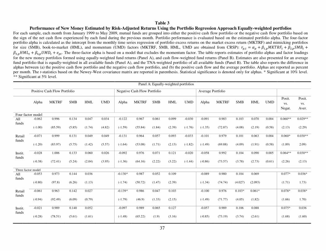
37

Table 3

Performance of New Money Estimated by Risk-Adjusted Returns Using the Portfolio Regression Approach Equally-weighted portfolios For each sample, each month from January 1999 to May 2009, mutual funds are grouped into either the positive cash flow portfolio or the negative cash flow portfolio based on the sign of the net cash flow experienced by each fund during the previous month. Portfolio performance is evaluated based on the estimated portfolio alpha. The four-factor portfolio alpha is calculated as the intercept from the monthly time series regression of portfolio excess returns on the market excess return (MKTRF) and mimicking portfolios for size (SMB), book-to-market (HML), and momentum (UMD) factors (MKTRF, SMB, HML, UMD are obtained from CRSP): (�,� = �� + ��,�� + ��,�� +��,�� + ��,� �!� + )��. The three-factor alpha is based on a model that excludes the momentum factor. The table reports estimates of portfolio alphas and factor loadings

for the new money portfolios formed using equally-weighted fund returns (Panel A), and cash flow-weighted fund returns (Panel B). Estimates are also presented for an average fund portfolio that is equally-weighted in all available funds (Panel A), and the TNA-weighted portfolio of all available funds (Panel B). The table also reports the difference in alphas between (a) the positive cash flow portfolio and the negative cash flow portfolio, and (b) the positive cash flow and the average portfolio. Alphas are reported as percent per month. The t-statistics based on the Newey-West covariance matrix are reported in parenthesis. Statistical significance is denoted only for alphas. * Significant at 10% level. ** Significant at 5% level.

Panel A: Equally-weighted portfolios

Positive Cash Flow Portfolio Negative Cash Flow Portfolio Average Portfolio

Alpha MKTRF SMB HML UMD Alpha MKTRF SMB HML UMD Alpha MKTRF SMB HML UMD

Posit.

vs.

Negat.

Posit.

vs.

Aver.

Four factor model All funds

-0.062 0.996 0.134 0.047 0.034 -0.122 0.967 0.061 0.099 -0.030 -0.091 0.983 0.103 0.070 0.004 0.060** 0.029**

(-1.00) (85.59) (5.85) (1.74) (4.82) (-1.59) (55.84) (1.84) (2.39) (-1.76) (-1.35) (72.87) (4.08) (2.19) (0.58) (2.13) (2.29)

Retail funds

-0.071 0.999 0.131 0.049 0.049 -0.131 0.964 0.057 0.093 -0.033 -0.101 0.979 0.101 0.063 0.004 0.060* 0.030**

(-1.20) (83.97) (5.75) (1.42) (5.57) (-1.64) (53.08) (1.71) (2.13) (-1.82) (-1.49) (69.88) (4.09) (1.91) (0.58) (1.89) 2.09)

Instit. funds

-0.028 1.006 0.133 0.060 0.026 -0.092 0.976 0.071 0.121 -0.020 -0.058 0.992 0.104 0.090 0.005 0.064** 0.030**

(-0.38) (72.41) (5.24) (2.04) (3.95) (-1.36) (64.16) (2.22) (3.22) (-1.44) (-0.86) (73.57) (3.78) (2.73) (0.61) (2.26) (2.13)

Three factor model

All funds

-0.053 0.973 0.144 0.036 -0.130* 0.987 0.052 0.109 -0.089 0.980 0.104 0.069 0.077* 0.036*

(-0.80) (97.8) (6.26) (1.13) (-1.74) (50.72) (1.47) (2.39) (-1.34) (74.74) (4.027) (2.093) (1.71) 1.73)

Retail funds

-0.061 0.963 0.142 0.027 -0.139* 0.986 0.047 0.103 -0.100 0.976 0.103* 0.061* 0.078* 0.038*

(-0.94) (92.49) (6.09) (0.79) (-1.79) (46.9) (1.33) (2.15) (-1.49) (71.77) (4.05) (1.82) (1.66) 1.70)

Instit. funds

-0.021 0.989 0.140 0.052 -0.097 0.989 0.065 0.127 -0.057 0.989 0.106 0.088 0.075* 0.036

(-0.28) (78.51) (5.61) (1.61) (-1.48) (65.22) (1.9) (3.16) (-0.85) (73.19) (3.74) (2.61) (1.68) (1.60)

38

Panel B: Cash flow-weighted portfolios

Positive Cash Flow Portfolio Negative Cash Flow Portfolio Average Portfolio

Alpha MKTRF SMB HML UMD Alpha MKTRF SMB HML UMD Alpha MKTRF SMB HML UMD

Posit.

vs.

Negat.

Posit.

vs.

Aver.

Four factor model

All funds -0.052 0.992 0.146 -0.012 0.075 -0.133* 0.964 -0.023 0.085 -0.053 -0.087** 0.979 0.026 0.022 0.009 0.081 0.035

(-1.52) (108.6) (6.90 (-0.47) (5.65) (-1.81) (52.02) (-0.67) (2.20) (-2.86) (-2.22) (102.8) (2.17) (1.29) (1.59) (1.36) (1.32)

Retail funds -0.038 0.981 0.147 -0.029 0.088 -0.125 0.963 -0.036 0.067 -0.057 -0.080* 0.978 0.024 0.012 0.012 0.087 0.042

(-0.95) (101.4) (5.85) (-1.00) (5.81) (-1.58) (49.63) (-1.05) (1.69) (-2.95) (-1.92) (101.4) (2.26) (0.61) (1.76) (1.34) (1.59)

Instit. funds -0.0531 0.995 0.115 0.0227 0.037 -0.146** 0.963 0.026 0.140 -0.038 -0.103*** 0.978 0.029 0.068 -0.005 0.093** 0.050*

(-1.63) (140.2) (7.01) (1.18) (6.30) (-2.54) (58.8) (0.81) (4.11) (-2.56) (-3.85) (87.55) (1.47) (3.56) (-0.95) (2.18) (1.78)

Three-factor model

All funds -0.033 0.942 0.168 -0.036 -0.147** 1.000 -0.038 0.103 -0.085** 0.973 0.029 0.019 0.114 0.052

(-0.55) (75.34) (6.85) (-0.83) (-2.01) (45.52 (-1.01) (2.31) (-2.17) (147.5) (2.41) (1.12) (1.28) (1.03)

Retail funds -0.016 0.923 0.172 0.058 -0.139* 1.001 -0.053 0.088 -0.078* 0.970 0.028 0.008 0.123 0.061

(-0.24) (69.22) (5.70) (-1.12) (-1.76) (43.27) (-1.37) (1.86) (-1.85) (158.8) (2.58) (0.42) (1.27) (1.16)

Instit. funds -0.044 0.971 0.125 0.011 -0.156*** 0.988 0.015 0.153 -0.104*** 0.982 0.027 0.070 0.112* 0.060

(-1.01) (142.5) (7.35) (0.41) (-2.74) (56.32) (0.43) (4.16) (-3.96) (85.4) (1.32) (3.55) (1.84) (1.41)

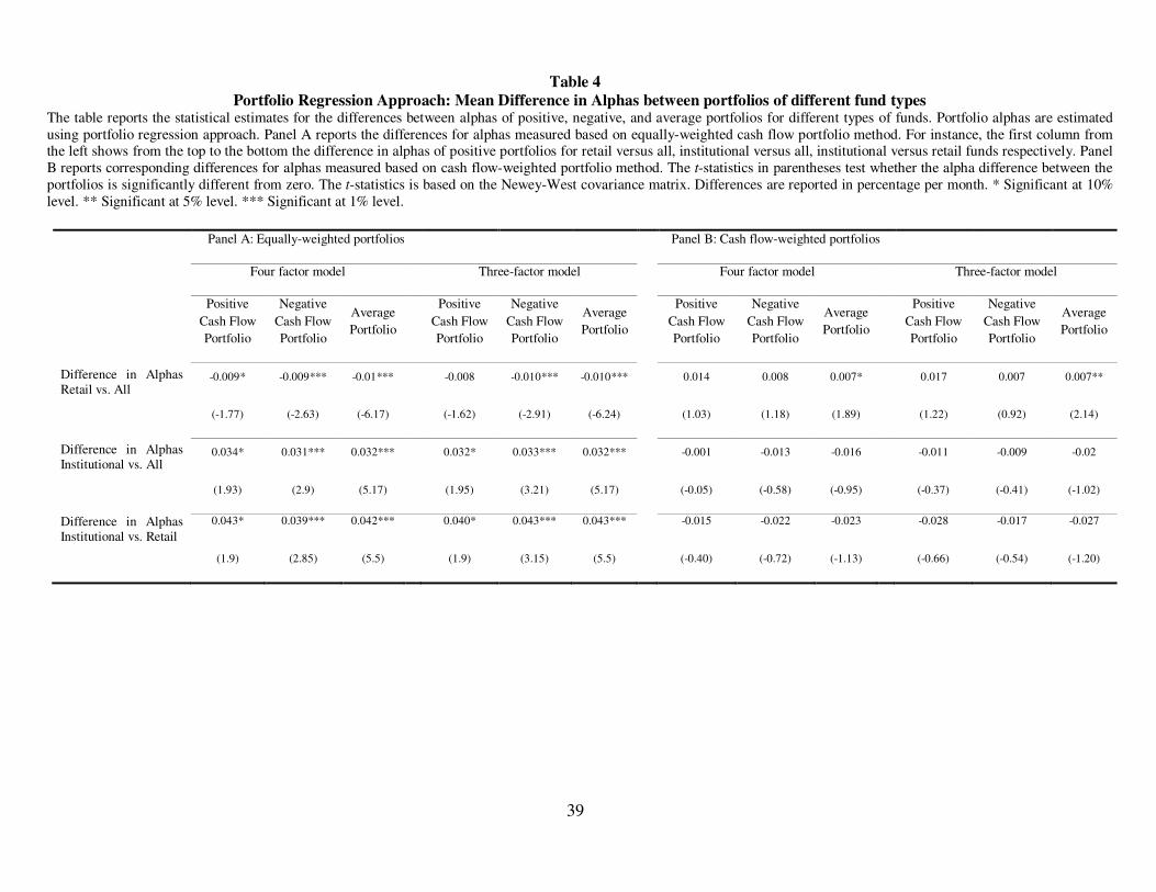
39

Table 4

Portfolio Regression Approach: Mean Difference in Alphas between portfolios of different fund types The table reports the statistical estimates for the differences between alphas of positive, negative, and average portfolios for different types of funds. Portfolio alphas are estimated using portfolio regression approach. Panel A reports the differences for alphas measured based on equally-weighted cash flow portfolio method. For instance, the first column from the left shows from the top to the bottom the difference in alphas of positive portfolios for retail versus all, institutional versus all, institutional versus retail funds respectively. Panel B reports corresponding differences for alphas measured based on cash flow-weighted portfolio method. The t-statistics in parentheses test whether the alpha difference between the portfolios is significantly different from zero. The t-statistics is based on the Newey-West covariance matrix. Differences are reported in percentage per month. * Significant at 10% level. ** Significant at 5% level. *** Significant at 1% level.

Panel A: Equally-weighted portfolios Panel B: Cash flow-weighted portfolios

Four factor model Three-factor model Four factor model Three-factor model

Positive

Cash Flow

Portfolio

Negative

Cash Flow

Portfolio

Average

Portfolio

Positive

Cash Flow

Portfolio

Negative

Cash Flow

Portfolio

Average

Portfolio

Positive

Cash Flow

Portfolio

Negative

Cash Flow

Portfolio

Average

Portfolio

Positive

Cash Flow

Portfolio

Negative

Cash Flow

Portfolio

Average

Portfolio

Difference in Alphas Retail vs. All

-0.009* -0.009*** -0.01*** -0.008 -0.010*** -0.010*** 0.014 0.008 0.007* 0.017 0.007 0.007**

(-1.77) (-2.63) (-6.17) (-1.62) (-2.91) (-6.24) (1.03) (1.18) (1.89) (1.22) (0.92) (2.14)

Difference in Alphas Institutional vs. All

0.034* 0.031*** 0.032*** 0.032* 0.033*** 0.032*** -0.001 -0.013 -0.016 -0.011 -0.009 -0.02

(1.93) (2.9) (5.17) (1.95) (3.21) (5.17) (-0.05) (-0.58) (-0.95) (-0.37) (-0.41) (-1.02)

Difference in Alphas Institutional vs. Retail

0.043* 0.039*** 0.042*** 0.040* 0.043*** 0.043*** -0.015 -0.022 -0.023 -0.028 -0.017 -0.027

(1.9) (2.85) (5.5) (1.9) (3.15) (5.5) (-0.40) (-0.72) (-1.13) (-0.66) (-0.54) (-1.20)

40

Table 5

Portfolio Regression Approach: Mean Difference in (Alpha of Positive Portfolio - Alpha of Negative Portfolio), and in (Alpha of Positive Portfolio

- Alpha of Average Portfolio) for different fund types The table reports the statistical estimates for the differences between each two types of funds in alpha difference of positive versus negative, and positive versus average portfolios. Portfolio alphas are estimated using portfolio regression approach. Panel A reports the differences for alphas measured based on equally-weighted cash flow portfolio method. For instance, the first column from the left shows from the top to the bottom respectively the difference between retail versus all, institutional versus all, and institutional versus retail funds in alpha difference of positive versus negative portfolios. Panel B reports corresponding differences for alphas measured based on cash flow-weighted portfolio method. The t-statistics in parentheses test whether the difference is significantly different from zero. The t-statistics is based on the Newey-West covariance matrix. Differences are reported in percentage per month. * Significant at 10% level. ** Significant at 5% level. *** Significant at 1% level.



Positive vs.

Negative

Positive vs.

Average

Positive vs.

Negative

Positive vs.

Average

Positive vs.

Negative

Positive vs.

Average

Positive vs.

Negative

Positive vs.

Average

Difference in “VS” Alphas Retail vs. All

-0.001 0.001 0.001 0.002 0.006 0.007 0.010 0.010

(-0.02) (0.32) (0.22) (0.47) (0.37) (0.55) (0.51) (0.64)

Difference in “VS” Alphas Institutional vs. All

0.003 0.002 -0.001 -0.001 0.012 0.015 -0.001 0.009

(0.16) (0.17) (-0.05) (-0.05) (0.30) (0.61) (-0.03) (0.29)

Difference in “VS” Alphas Institutional vs. Retail

0.003 0.001 -0.003 -0.003 0.007 0.008 -0. 011 -0.001

(0.13) (0.04) (-0.09) (-0.19) (0.12) (0.22) (-0.16) (-0.03)

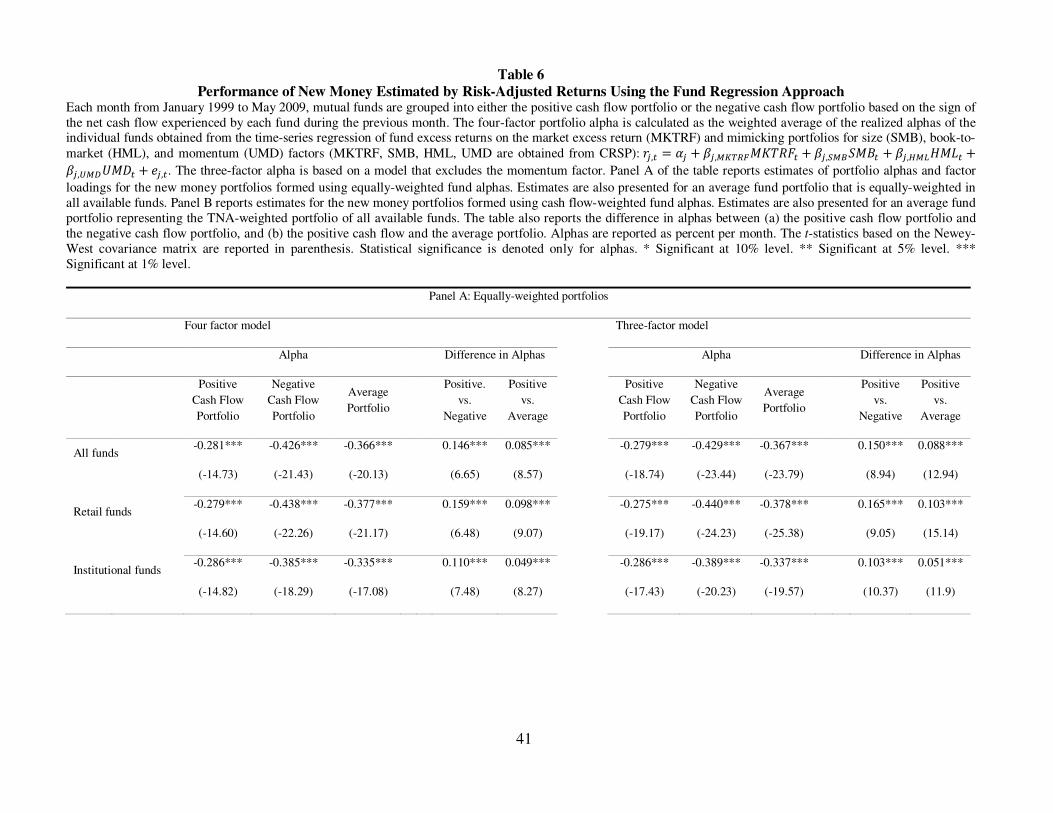
41

Table 6

Performance of New Money Estimated by Risk-Adjusted Returns Using the Fund Regression Approach Each month from January 1999 to May 2009, mutual funds are grouped into either the positive cash flow portfolio or the negative cash flow portfolio based on the sign of the net cash flow experienced by each fund during the previous month. The four-factor portfolio alpha is calculated as the weighted average of the realized alphas of the individual funds obtained from the time-series regression of fund excess returns on the market excess return (MKTRF) and mimicking portfolios for size (SMB), book-to-market (HML), and momentum (UMD) factors (MKTRF, SMB, HML, UMD are obtained from CRSP): (�,� = �� + ��,+,-./�� + ��,0+1�� + ��,2+3�� +��,4+5 �!� + )�,�. The three-factor alpha is based on a model that excludes the momentum factor. Panel A of the table reports estimates of portfolio alphas and factor

loadings for the new money portfolios formed using equally-weighted fund alphas. Estimates are also presented for an average fund portfolio that is equally-weighted in all available funds. Panel B reports estimates for the new money portfolios formed using cash flow-weighted fund alphas. Estimates are also presented for an average fund portfolio representing the TNA-weighted portfolio of all available funds. The table also reports the difference in alphas between (a) the positive cash flow portfolio and the negative cash flow portfolio, and (b) the positive cash flow and the average portfolio. Alphas are reported as percent per month. The t-statistics based on the Newey-West covariance matrix are reported in parenthesis. Statistical significance is denoted only for alphas. * Significant at 10% level. ** Significant at 5% level. *** Significant at 1% level.

Panel A: Equally-weighted portfolios

Four factor model Three-factor model

Alpha Difference in Alphas Alpha Difference in Alphas

Positive

Cash Flow

Portfolio

Negative

Cash Flow

Portfolio

Average

Portfolio

Positive.

vs.

Negative

Positive

vs.

Average

Positive

Cash Flow

Portfolio

Negative

Cash Flow

Portfolio

Average

Portfolio

Positive

vs.

Negative

Positive

vs.

Average

All funds -0.281*** -0.426*** -0.366*** 0.146*** 0.085*** -0.279*** -0.429*** -0.367*** 0.150*** 0.088***

(-14.73) (-21.43) (-20.13) (6.65) (8.57) (-18.74) (-23.44) (-23.79) (8.94) (12.94)

Retail funds -0.279*** -0.438*** -0.377*** 0.159*** 0.098*** -0.275*** -0.440*** -0.378*** 0.165*** 0.103***

(-14.60) (-22.26) (-21.17) (6.48) (9.07) (-19.17) (-24.23) (-25.38) (9.05) (15.14)

Institutional funds -0.286*** -0.385*** -0.335*** 0.110*** 0.049*** -0.286*** -0.389*** -0.337*** 0.103*** 0.051***

(-14.82) (-18.29) (-17.08) (7.48) (8.27) (-17.43) (-20.23) (-19.57) (10.37) (11.9)

42

Panel B: Cash flow-weighted portfolios

Four factor model Three-factor model

Alpha Difference in Alphas Alpha Difference in Alphas

Positive

Cash Flow

Portfolio

Negative

Cash Flow

Portfolio

Average

Portfolio

Positive.

vs.

Negative

Positive

vs.

Average

Positive

Cash Flow

Portfolio

Negative

Cash Flow

Portfolio

Average

Portfolio

Positive

vs.

Negative

Positive

vs.

Average

All funds -0.148*** -0.391*** -0.263*** 0.242*** 0.115*** -0.144*** -0.395*** -0.263*** 0.251*** 0.119***

(-6.18) (-19.52) (-16.95) (6.51) (5.21) (-7.95) (-19.88) (-20.11) (9.40) (7.07)

Retail funds -0.118*** -0.396*** -0.259*** 0.277*** 0.141*** -0.110*** -0.400*** -0.258*** 0.289*** 0.148***

(-4.636) (-18.81) (-17.06) (6.5) (5.24) (-5.764) (-19.15) (-20.71) (9.597) (7.22)

Institutional funds -0.217*** -0.372*** -0.282*** 0.156*** 0.065*** -0.217*** -0.380*** -0.286*** 0.163*** 0.069***

(-11.92) (-20.03) (-17.39) (11.35) (13.75) (-14.41) (-19.63) (-19.18) (18.44) (16.96)

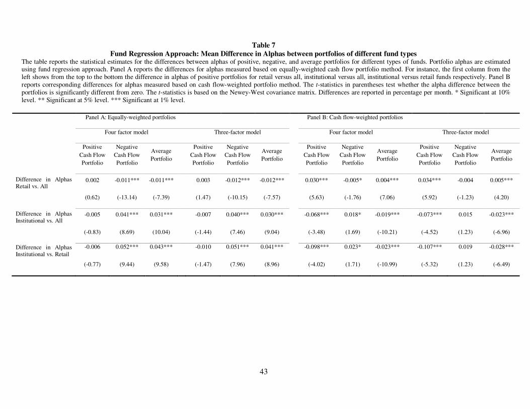
43

Table 7

Fund Regression Approach: Mean Difference in Alphas between portfolios of different fund types The table reports the statistical estimates for the differences between alphas of positive, negative, and average portfolios for different types of funds. Portfolio alphas are estimated using fund regression approach. Panel A reports the differences for alphas measured based on equally-weighted cash flow portfolio method. For instance, the first column from the left shows from the top to the bottom the difference in alphas of positive portfolios for retail versus all, institutional versus all, institutional versus retail funds respectively. Panel B reports corresponding differences for alphas measured based on cash flow-weighted portfolio method. The t-statistics in parentheses test whether the alpha difference between the portfolios is significantly different from zero. The t-statistics is based on the Newey-West covariance matrix. Differences are reported in percentage per month. * Significant at 10% level. ** Significant at 5% level. *** Significant at 1% level.



Positive

Cash Flow

Portfolio

Negative

Cash Flow

Portfolio

Average

Portfolio

Positive

Cash Flow

Portfolio

Negative

Cash Flow

Portfolio

Average

Portfolio

Positive

Cash Flow

Portfolio

Negative

Cash Flow

Portfolio

Average

Portfolio

Positive

Cash Flow

Portfolio

Negative

Cash Flow

Portfolio

Average

Portfolio

Difference in Alphas Retail vs. All

0.002 -0.011*** -0.011*** 0.003 -0.012*** -0.012*** 0.030*** -0.005* 0.004*** 0.034*** -0.004 0.005***

(0.62) (-13.14) (-7.39) (1.47) (-10.15) (-7.57) (5.63) (-1.76) (7.06) (5.92) (-1.23) (4.20)

Difference in Alphas Institutional vs. All

-0.005 0.041*** 0.031*** -0.007 0.040*** 0.030*** -0.068*** 0.018* -0.019*** -0.073*** 0.015 -0.023***

(-0.83) (8.69) (10.04) (-1.44) (7.46) (9.04) (-3.48) (1.69) (-10.21) (-4.52) (1.23) (-6.96)

Difference in Alphas Institutional vs. Retail

-0.006 0.052*** 0.043*** -0.010 0.051*** 0.041*** -0.098*** 0.023* -0.023*** -0.107*** 0.019 -0.028***

(-0.77) (9.44) (9.58) (-1.47) (7.96) (8.96) (-4.02) (1.71) (-10.99) (-5.32) (1.23) (-6.49)

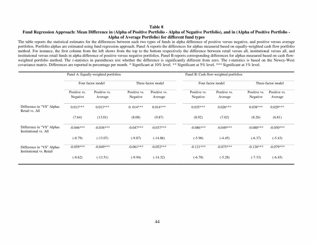
44

Table 8

Fund Regression Approach: Mean Difference in (Alpha of Positive Portfolio - Alpha of Negative Portfolio), and in (Alpha of Positive Portfolio -

Alpha of Average Portfolio) for different fund types The table reports the statistical estimates for the differences between each two types of funds in alpha difference of positive versus negative, and positive versus average portfolios. Portfolio alphas are estimated using fund regression approach. Panel A reports the differences for alphas measured based on equally-weighted cash flow portfolio method. For instance, the first column from the left shows from the top to the bottom respectively the difference between retail versus all, institutional versus all, and institutional versus retail funds in alpha difference of positive versus negative portfolios. Panel B reports corresponding differences for alphas measured based on cash flow-weighted portfolio method. The t-statistics in parentheses test whether the difference is significantly different from zero. The t-statistics is based on the Newey-West covariance matrix. Differences are reported in percentage per month. * Significant at 10% level. ** Significant at 5% level. *** Significant at 1% level.



Positive vs.

Negative

Positive vs.

Average

Positive vs.

Negative

Positive vs.

Average

Positive vs.

Negative

Positive vs.

Average

Positive vs.

Negative

Positive vs.

Average

Difference in “VS” Alphas Retail vs. All

0.013*** 0.013*** 0. 014*** 0.014*** 0.035*** 0.026*** 0.038*** 0.029***

(7.64) (13.01) (8.08) (9.87) (8.92) (7.02) (8.26) (6.81)

Difference in “VS” Alphas Institutional vs. All

-0.046*** -0.036*** -0.047*** -0.037*** -0.086*** -0.049*** -0.088*** -0.050***

(-8.79) (-13.07) (-9.87) (-14.86) (-5.96) (-4.45) (-6.37) (-5.43)

Difference in “VS” Alphas Institutional vs. Retail

-0.059*** -0.049*** -0.061*** -0.052*** -0.121*** -0.075*** -0.126*** -0.079***

(-8.62) (-13.51) (-9.94) (-14.32) (-6.78) (-5.28) (-7.33) (-6.45)

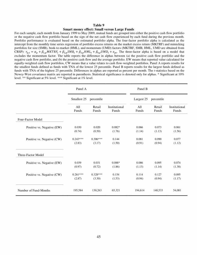
45

Table 9

Smart money effect: Small versus Large Funds For each sample, each month from January 1999 to May 2009, mutual funds are grouped into either the positive cash flow portfolio or the negative cash flow portfolio based on the sign of the net cash flow experienced by each fund during the previous month. Portfolio performance is evaluated based on the estimated portfolio alpha. The four-factor portfolio alpha is calculated as the intercept from the monthly time series regression of portfolio excess returns on the market excess return (MKTRF) and mimicking portfolios for size (SMB), book-to-market (HML), and momentum (UMD) factors (MKTRF, SMB, HML, UMD are obtained from CRSP): (�,� = �� + ��,�� + ��,�� + ��,�� + ��,� �!� + )��. The three-factor alpha is based on a model that

excludes the momentum factor. The table reports the difference in alphas between (a) the positive cash flow portfolio and the negative cash flow portfolio, and (b) the positive cash flow and the average portfolio. EW means that reported value calculated for equally-weighted cash flow portfolios, CW means that a value relates to cash flow-weighted portfolios. Panel A reports results for the smallest funds defined as funds with TNA of the lowest 25 percentile. Panel B reports results for the largest funds defined as funds with TNA of the highest 25 percentile. Differences in alphas are reported as percent per month. The t-statistics based on the Newey-West covariance matrix are reported in parenthesis. Statistical significance is denoted only for alphas. * Significant at 10% level. ** Significant at 5% level. *** Significant at 1% level.

Panel A Panel B

Smallest 25 percentile Largest 25 percentile

All Funds

Retail Funds

Institutional Funds

All

Funds Retail Funds

Institutional Funds

Four-Factor Model

Positive vs. Negative (EW) 0.030 0.020 0.082* 0.066 0.073 0.061

(0.74) (0.50) (1.76) (1.14) (1.13) (1.56)

Positive vs. Negative (CW) 0.243*** 0.306*** 0.144 0.081 0.090 0.077

(2.83) (3.17) (1.50) (0.91) (0.94) (1.12)

Three-Factor Model

Positive vs. Negative (EW) 0.039 0.031 0.088* 0.086 0.095 0.074

(0.97) (0.72) (1.86) (1.13) (1.14) (1.38)

Positive vs. Negative (CW) 0.261*** 0.328*** 0.154 0.114 0.127 0.095

(2.87) (3.30) (1.53) (0.94) (0.94) (1.17)

Number of Fund-Months 195,584 130,263 65,321 194,614 140,533 54,081

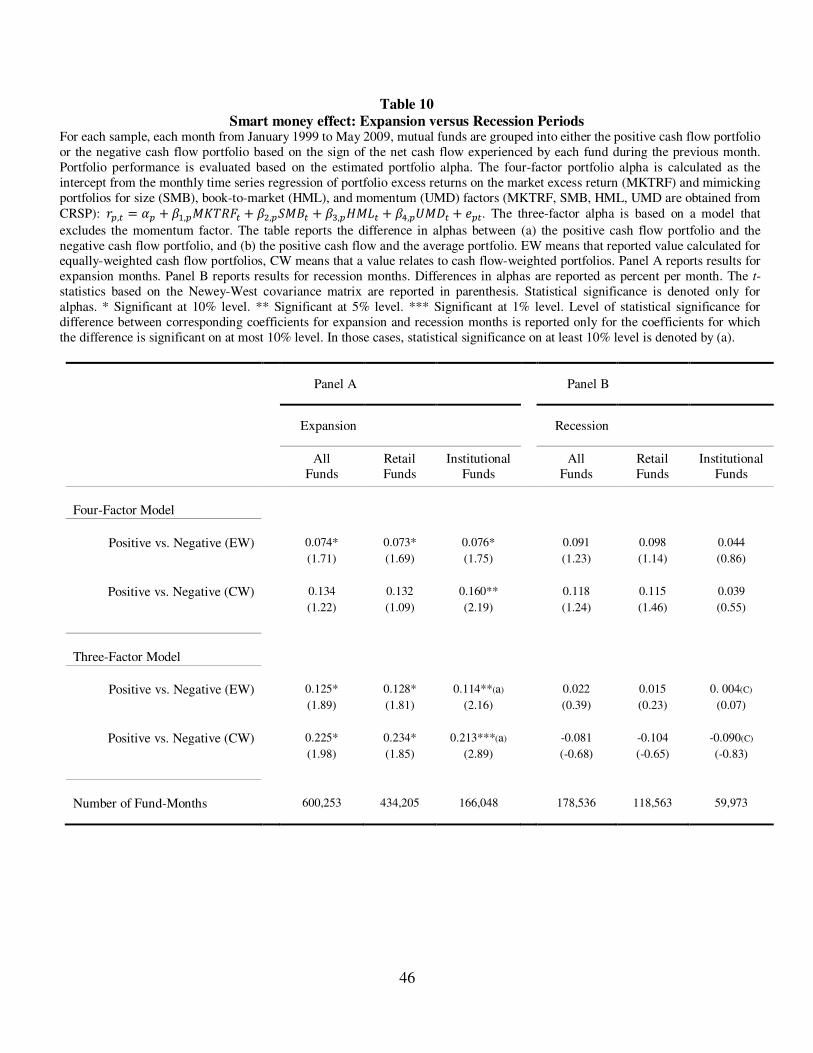
46

Table 10

Smart money effect: Expansion versus Recession Periods For each sample, each month from January 1999 to May 2009, mutual funds are grouped into either the positive cash flow portfolio or the negative cash flow portfolio based on the sign of the net cash flow experienced by each fund during the previous month. Portfolio performance is evaluated based on the estimated portfolio alpha. The four-factor portfolio alpha is calculated as the intercept from the monthly time series regression of portfolio excess returns on the market excess return (MKTRF) and mimicking portfolios for size (SMB), book-to-market (HML), and momentum (UMD) factors (MKTRF, SMB, HML, UMD are obtained from CRSP): (�,� = �� + ��,�� + ��,�� + ��,�� + ��,� �!� + )��. The three-factor alpha is based on a model that

excludes the momentum factor. The table reports the difference in alphas between (a) the positive cash flow portfolio and the negative cash flow portfolio, and (b) the positive cash flow and the average portfolio. EW means that reported value calculated for equally-weighted cash flow portfolios, CW means that a value relates to cash flow-weighted portfolios. Panel A reports results for expansion months. Panel B reports results for recession months. Differences in alphas are reported as percent per month. The t-statistics based on the Newey-West covariance matrix are reported in parenthesis. Statistical significance is denoted only for alphas. * Significant at 10% level. ** Significant at 5% level. *** Significant at 1% level. Level of statistical significance for difference between corresponding coefficients for expansion and recession months is reported only for the coefficients for which the difference is significant on at most 10% level. In those cases, statistical significance on at least 10% level is denoted by (a).

Panel A Panel B

Expansion Recession

All Funds

Retail Funds

Institutional Funds

All

Funds Retail Funds

Institutional Funds

Four-Factor Model

Positive vs. Negative (EW) 0.074* 0.073* 0.076* 0.091 0.098 0.044

(1.71) (1.69) (1.75) (1.23) (1.14) (0.86)

Positive vs. Negative (CW) 0.134 0.132 0.160** 0.118 0.115 0.039

(1.22) (1.09) (2.19) (1.24) (1.46) (0.55)

Three-Factor Model

Positive vs. Negative (EW) 0.125* 0.128* 0.114**(a) 0.022 0.015 0. 004(C)

(1.89) (1.81) (2.16) (0.39) (0.23) (0.07)

Positive vs. Negative (CW) 0.225* 0.234* 0.213***(a) -0.081 -0.104 -0.090(C)

(1.98) (1.85) (2.89) (-0.68) (-0.65) (-0.83)

Number of Fund-Months 600,253 434,205 166,048 178,536

118,563 59,973

47

Table 11

Determinants of Net Cash Flows: Retail versus Institutional Funds The table reports the coefficients from pooled time-series cross-sectional OLS regressions of funds’ monthly net cash flow on the momentum (UMD) loading calculated over the previous 36 month of fund return, fund total net assets estimated to the end of the previous month, the 1st lag of fund’s annual return, fund risk estimated as the standard deviation of fund return over the previous 12 months, the monthly normalized cash flow of fund’s IOC, turnover ratios defined as a minimum of aggregate purchases or sales of securities during the year, divided by average fund total net assets, fund expense ratio is the percentage of total investment that shareholders pay for the fund’s operating expenses. I also include time-style interaction dummies for each combination of month and style. Panel A (Specification (1)) reports the results for all funds in the sample. Panel B (Specification (2)) reports the results of the regression in which I interact each of the explanatory variables once with a dummy identifying retail funds and once more time with the dummy identifying institutional funds. I also include the dummy identifying institutional funds as a separate variable. The columns titled “Difference Institutional vs. Retail” reports differences between the coefficients of institutional and retail funds from the regression analysis summarized in Specification (2), exhibiting the difference in effect of respective variable on fund money flows of the two types of funds. The t-statistics are reported in parentheses. The standard errors are clustered by funds. * Significant at 10% level. ** Significant at 5% level. *** Significant at 1% level.

Panel A

Panel B

(1)

(2)

All

Funds

Retail Funds

Intuitional Funds

Difference Institutional vs.

Retail

Intercept/ Institutional Dummy 5.111*** 3.090** 3.044* 3.044* (4.28) (2.24) (1.99) (1.99)

UMD Loading 4.238*** 3.962*** 6.601*** 2.639*

(4.49) (3.59) (5.22) (1.72)

Fund’s Total Net Assets 0.0002 0.0001 0.0074*** 0.0074***

(0.56) (-0.24) (5.78) (5.59)

Lagged Annual Return 0.315*** 0.329*** 0.257*** -0.072***

(18.25) (17.83) (15.17) (-5.90)

Fund Risk 0.083*** 0.118*** -0.054 -0.172***

(2.30) (2.96) (-1.35) (-4.07)

IOC Net Cash Flow 0.001*** 0.002*** 0.001*** -0.001***

(8.59) (8.83) (4.68) (-4.76)

Turnover Ratio -0.012*** -0.008*** -0.009*** -0.001

(-4.95) (-2.83) (-2.76) (-0.15)

Expense Ratio -1.756*** -1.250*** -0.200 1.050

(-6.33) (-3.09) (-0.33) (1.44)

Fund Age -0.025*** -0.021*** -0.053*** -0.032***

(-6.57) (-5.26) (-5.69) (-3.20)

R sq. adjusted 0.030 0.049 No. Fund-Months/Entities 7,995 7,995 No. Fund- Entities 393,360 393,360

48

Figure 1 Number of Mutual Funds over the period between January 1999 and May 2009

Figure 2 Cumulative Monthly Total Net Asset Value (in millions of U.S. dollar) of corresponding group of Mutual Funds over the period between January 1999 and May 2009

0

1,000

2,000

3,000

4,000

5,000

6,000

7,000

8,000

9,000

Jan

/99

Jul/

99

Jan

/00

Jul/

00

Jan

/01

Jul/

01

Jan

/02

Jul/

02

Jan

/03

Jul/

03

Jan

/04

Jul/

04

Jan

/05

Jul/

05

Jan

/06

Jul/

06

Jan

/07

Jul/

07

Jan

/08

Jul/

08

Jan

/09

All Funds Retail Funds Institutional Funds

0

500,000

1,000,000

1,500,000

2,000,000

2,500,000

3,000,000

3,500,000

4,000,000

4,500,000

Jan

/99

Jul/

99

Jan

/00

Jul/

00

Jan

/01

Jul/

01

Jan

/02

Jul/

02

Jan

/03

Jul/

03

Jan

/04

Jul/

04

Jan

/05

Jul/

05

Jan

/06

Jul/

06

Jan

/07

Jul/

07

Jan

/08

Jul/

08

Jan

/09


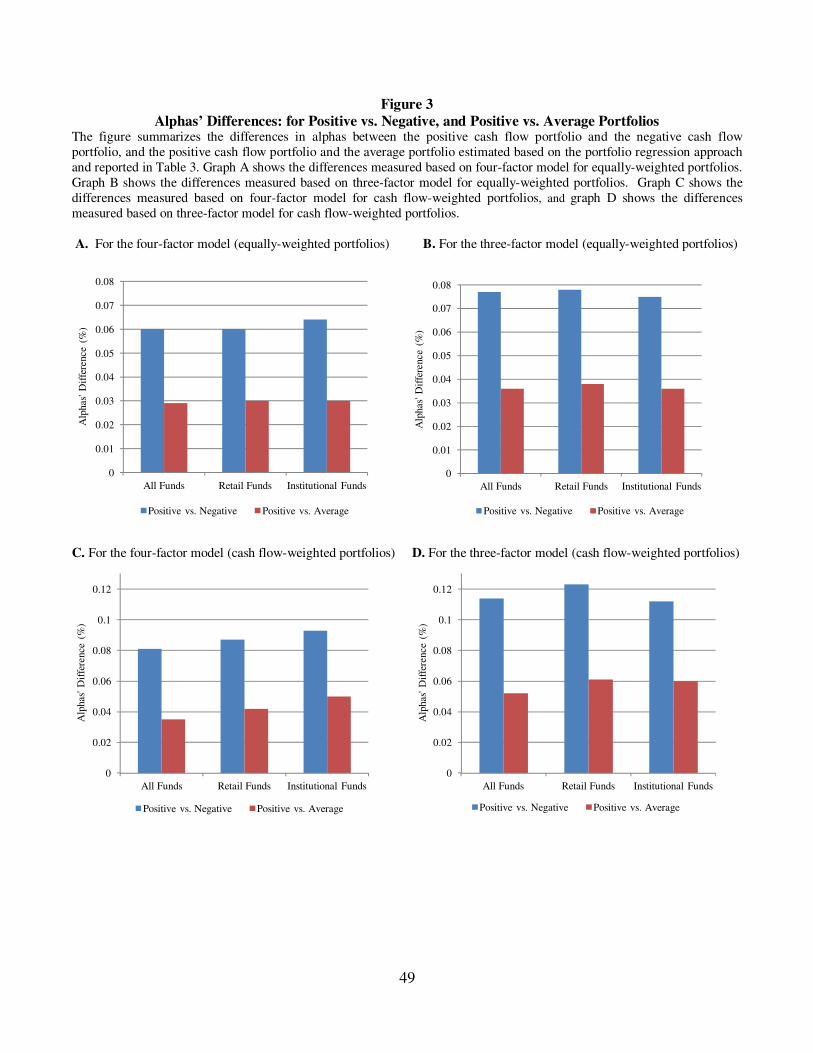
49

Figure 3

Alphas’ Differences: for Positive vs. Negative, and Positive vs. Average Portfolios The figure summarizes the differences in alphas between the positive cash flow portfolio and the negative cash flow portfolio, and the positive cash flow portfolio and the average portfolio estimated based on the portfolio regression approach and reported in Table 3. Graph A shows the differences measured based on four-factor model for equally-weighted portfolios. Graph B shows the differences measured based on three-factor model for equally-weighted portfolios. Graph C shows the differences measured based on four-factor model for cash flow-weighted portfolios, and graph D shows the differences measured based on three-factor model for cash flow-weighted portfolios.

A. For the four-factor model (equally-weighted portfolios) B. For the three-factor model (equally-weighted portfolios)

C. For the four-factor model (cash flow-weighted portfolios) D. For the three-factor model (cash flow-weighted portfolios)

0

0.01

0.02

0.03

0.04

0.05

0.06

0.07

0.08


Alp

has

' D

iffe

rence

(%

)

Positive vs. Negative Positive vs. Average

0

0.01

0.02

0.03

0.04

0.05

0.06

0.07

0.08


Alp

has

' D

iffe

rence

(%

)


0

0.02

0.04

0.06

0.08

0.1

0.12


Alp

has

' D

iffe

rence

(%

)


0

0.02

0.04

0.06

0.08

0.1

0.12


Alp

has

' D

iffe

rence

(%

)


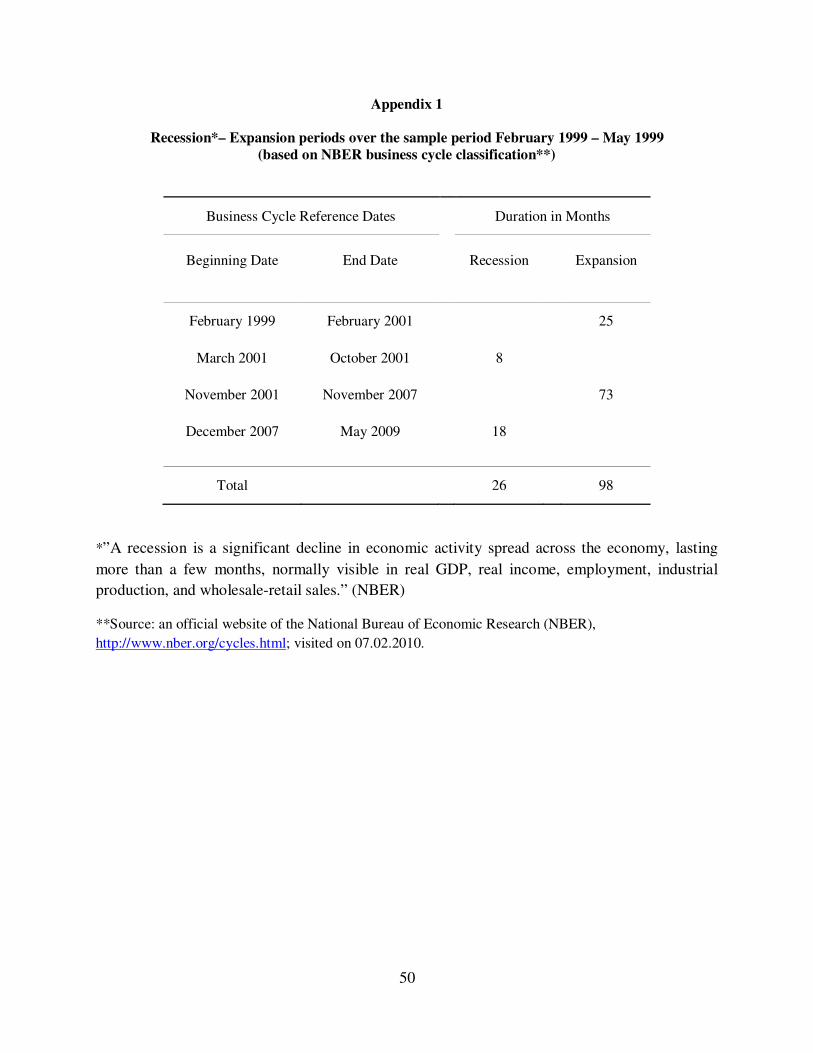
50

Appendix 1

Recession*– Expansion periods over the sample period February 1999 – May 1999

(based on NBER business cycle classification**)

Business Cycle Reference Dates Duration in Months

Beginning Date End Date

Recession Expansion

February 1999 February 2001 25

March 2001 October 2001 8

November 2001 November 2007 73

December 2007 May 2009 18

Total 26 98

*”A recession is a significant decline in economic activity spread across the economy, lasting

more than a few months, normally visible in real GDP, real income, employment, industrial

production, and wholesale-retail sales.” (NBER)

**Source: an official website of the National Bureau of Economic Research (NBER),

http://www.nber.org/cycles.html; visited on 07.02.2010.

the “smart money” effect: retail versus institutional

Documents