UPTEC W10 012

Examensarbete 30 hpMaj 2010

The sodar as a screening instrument

Comparison with cup anemometer measurements

and long-term correction studies

Anders Nilsson

i

ABSTRACT

The sodar as a screening instrument - Comparison with cup anemometer measure-

ments and long-term correction studies

Anders Nilsson

A site assessment including wind measurements is of major importance when planning

a wind farm. Small differences in wind speed can determine if a project will be eco-

nomically viable since the power in the wind is proportional to the cube of the wind

speed. It is also important to have knowledge about the long-term wind climate since

the technical lifetime of a wind turbine is about 20 - 25 years.

Traditionally, masts mounted with cup anemometers and wind wanes have been used

for wind measurements during site assessments. However, an instrument called sodar

which measures the wind based on sound waves has entered the market some years ago

and offers some advantages in terms of e.g. mobility compared to the mast equipped

with cup anemometers and wind vanes. Since the sodar is a relatively new instrument in

the wind energy business, it is important to gain knowledge on how the instrument

operates and its performance. To do that, sodar measurements have been compared to

wind measurements performed by a cup anemometer and a wind vane.

In order to estimate the long-term wind climate at a site, a long-term calculation is

performed based on short-term measurements from the site and a long-term reference

wind data. At least one year of wind measurements at the site are needed in order to

obtain a valid result from the calculation. However, for an early evaluation of a site it is

desirable to measure the wind for a shorter period of time. Therefore, it has been studied

in this thesis how the result of the long-term correction depends on the length of the site

measurement period. The seasonal impact on the results has also been studied to

distinguish what season is the most suitable for short measurements.

According to the results, the measurements performed by the sodar used in this study

are as valid as those performed by the cup anemometer and the wind vane. Considering

the advantages with the sodar compared to the mast equipped with cup anemometers

and wind vanes, the sodar is the preferable choice.

The results from the long-term correction calculations improve most rapidly during the

first four months of measurements. It is therefore important to measure the wind for at

least four months. Best results are obtained when the measurements are performed

during the spring and the autumn compared to the summer and the winter.

Keywords: Sodar, long-term correction, wind measurement, wind power

Department of Earth Sciences, Program for Air, Water and Landscape Science.

Uppsala University. Geocentrum, Villavägen 16, SE-752 36 UPPSALA

ISSN 1401-5765

ii

REFERAT

Sodar som ett screeninginstrument - Jämförelse mot mätningar med skålkorsane-

mometer och studier av långtidskorrigeringar.

Anders Nilsson

En platsbedömning innehållande vindmätningar är en mycket viktig del i projekteringen

av en vindkraftspark. Eftersom effekten i vinden är proportionell mot vindhastigheten i

kubik kan små variationer i vindhastighet avgöra om ett projekt blir ekonomiskt håll-

bart. Det är också viktigt att ha kunskap om det långsiktiga vindklimatet då ett vind-

kraftverks tekniska livslängd är 20 - 25 år.

Traditionellt sett har mätmaster utrustade med skålkorsanemometrar och vindfanor

använts för att mäta vinden vid platsbedömningar. För några år sedan har dock ett

mätinstrument som kallas sodar slagit sig in på marknaden. Detta instrument använder

en teknik som bygger på ljudvågor och erbjuder fördelar i t.ex. mobilitet jämfört med

mätmasten utrustad med skålkorsanemometrar och vindfanor. Då sodar är ett relativt

nytt instrument i vindkraftsbranschen är det viktigt att skaffa sig kunskap om hur

instrumentet fungerar och vilken prestanda det har. Av denna anledning har vindmät-

ningar med sodar jämförts med vindmätningar gjorda med skålkorsanemometer och

vindfana.

För att uppskatta det långsiktiga vindklimatet på en plats utförs en långtidskorrigering

baserad på kortidsmätningar från den aktuella platsen och vinddata från en längre tids-

period. Det krävs minst ett års vindmätningar från platsen för att erhålla säkra resultat

från långtidskorrigeringen, men för en tidig utvärdering är det önskvärt att mäta vinden

under en kortare period. Därmed har det i denna rapport studerats hur resultatet av en

långtidskorrektion beror av längden på mätperioden. Det har också studerats om det

finns ett årstidsberoende i resultatet som kan visa på vilken årstid som är mest lämpad

för korta mätningar.

Enligt resultaten håller vindmätningar utförda med den sodar som användes i denna

rapport lika hög prestanda som vindmätningar utförda med skålkorsanemometer och

vindfana. En sodar är då att föredra framför en mast utrustad med skålkorsanemometer

och vindfana med tanke på sodarinstrumentets praktiska fördelar.

Resultaten av långtidskorrektionerna förbättras markant under de fyra första månaderna

av mätningar vilket innebär att det är viktigt att mäta vinden i minst fyra månader. Bäst

resultat erhålls då mätningarna utförs under vår och höst jämfört med under sommar och

vinter.

Nyckelord: Sodar, långtidskorrektion, vindmätning, vindkraft

Institutionen för geovetenskaper, Luft- vatten- och landskapslära. Uppsala universitet

Geocentrum, Villavägen 16, SE-752 36 UPPSALA

ISSN 1401-5765

iii

PREFACE

This Master Thesis was performed at Nordex Sverige AB as a completion of the

Aquatic and Environmental Engineering program at Uppsala University. The thesis

comprises 30 ECTS. Supervisor was Kristian Baurne, Project Engineer at Nordex

Sverige AB and subject reviewer was Hans Bergström, PhD in meteorology at the

Department of Earth Science, Air, Water and Landscape Science, Uppsala University.

I would like to thank the team at Nordex Sverige AB for the good time at their office

and Michael Henriksson for providing me with this opportunity. Special thanks to

Kristian Baurne for excellent supervision and all the effort he has put in to my work. I

would also like to thank Hans Bergström, Mats Hurtig at AQSystem, Niklas Sondell at

Storm Weather Center, Frank Gross at Nordex Energy GmBH and Barry Neal at

Atmospheric Research & Technology, LLC, Hawaii for providing me with information

and valuable input. Finally, I would like to thank Beau Boekhout for many laughs at the

office and for proofreading of this report.

Uppsala 2010

Anders Nilsson

Copyright © Anders Nilsson and Department of Earth Sciences, Air, Water and

Landscape Science, Uppsala University

UPTEC W10 012, ISSN 1401‐5765

Printed at the Department of Earth Sciences, Geotryckeriet, Uppsala University,

Uppsala 2010

iv

POPULÄRVETENSKAPLIG SAMMANFATTNING

Sodar som ett screeninginstrument - Jämförelse mot mätningar med skålkorsane-

mometer och studier av långtidskorrigeringar.

Anders Nilsson

Vindkraft är en förnyelsebar energikälla där den kinetiska energin i vinden omvandlas

till elektricitet. 2008 var Sveriges årliga produktion av elektricitet från vindkraft är 1,6

TWh men regeringen har som mål med vindkraft att årligen producera 30 TWh år 2020.

Detta innebär att det planeras för en omfattande utbyggnad av vindkraften i Sverige.

När en vindkraftspark skall byggas är det viktigt att en utförlig platsbedömning genom-

förs. Denna platsbedömning består av allt från att beräkna ljudutbredning från verken

till att inventera fåglar och fladdermöss, men framförallt utförs vindmätningar för att

kunna beräkna hur mycket energi det går att få ut från den aktuella platsen. Om det inte

blåser tillräckligt mycket på den tänkta platsen är det ingen idé att bygga några

vindkraftverk då det inte kommer att vara ekonomiskt lönsamt. Eftersom vindkraftverk

har en livstid på 20 – 25 år är det viktigt att ha kännedom om det långsiktiga

vindklimatet då detta kan ändras mycket från år till år.

Vindmätningar har traditionellt sett utförts med mätmaster utrustade med skålkorsane-

mometrar och vindfanor på olika höjder. Nackdelen med denna metod är att den prak-

tiskt sett inte är mobil för att flyttas till en annan plats samt att den enbart ger uppgifter

om vindhastighet och vindriktning på de höjder som det finns mätutrustning på. Ett nytt

sätt att utvärdera vindklimatet på en plats är att använda en sodar. Sodar står för Sound

Detecting and Ranging och mäter vindhastighet och vindriktning genom att skicka ut

ljudpulser och analysera de mottagna ekona. Denna metod erbjuder en del fördelar

jämfört med det traditionella sättet att mäta vind på, bl.a. en vindprofil upp till 200 m

med ett värde för hastighet och riktning var femte meter. Eftersom en sodar ryms på en

släpvagn är den även mobil och kan lätt flyttas mellan olika platser.

Då det är otänkbart att mäta vinden under 20 – 25 år för att få kunskap om det lång-

siktiga vindklimatet på en plats utförs en så kallad långtidskorrigering av vinddata. I en

långtidskorrigering kombineras vindmätningen från den tänkta platsen med en vind-

referens som t.ex. kan vara en närliggande vindmätning som pågått under längre tid. På

så sätt kan man uppskatta det långsiktiga vindklimatet för en viss plats utan att mäta

vinden för hela den tiden.

Fördelarna med sodar gör instrumentet till ett intressant alternativ, men eftersom

tekniken är relativt ny i vindkraftssammanhang är det viktigt att lära sig hur instru-

mentet fungerar och att undersöka dess prestanda. I den här rapporten har detta gjorts

genom att studera litteratur om sodarteknik och genom att jämföra vindmätningar

utförda med sodar och med skålkorsanemometer samt vindfana monterade på en mät-

mast. Jämförelsen har skett på tre platser och de faktorer som har jämförts är vind-

hastighet, vindriktning, samt i viss mån turbulens.

v

För att erhålla säkra resultat av en långtidskorrektion måste mätperioden på platsen vara

minst ett år lång. Det är däremot önskvärt att få en tidigare uppfattning om vindklimatet

på platsen utan ett behöva vänta på mätningar i ett år. Med hjälp av en tidig uppskatt-

ning av vindklimatet kan en bedömning göras om det är lönt att fortsätta med projekt.

Därav har det i detta arbete studerats hur bra långtidskorrigeringar som är baserade på

färre antal månader än ett år stämmer överens med en långtidskorrigering som är base-

rad på ett år. Det har även studerats om olika årstider kan tänkas ha någon inverkan på

resultatet när en uppskattning av det långsiktiga vindklimatet baseras på kortare

mätperioder än ett år.

I dagsläget är inte vindmätningar utförda med enbart sodar accepterade av banker eller

vindkraftstillverkare, men eftersom en sodar är ett mobilt instrument skulle det kunna

användas som ett screeninginstrument i syfte att ge en tidig utvärdering om vindklimatet

på platsen.

Resultatet av jämförelsen mellan sodarmätningar och vindmätningar utförda med skål-

korsanemometer och vindfana visar att mätningar med sodar håller lika hög kvalitet

som mätningar med skålkorsanemometer och vindfana, vilka i dagsläget anses som

standard i branschen. På en av de tre platser som vindmätningar jämförts på var avstån-

det mellan sodar och mast så stort att inga slutsatser kunde dras men på de andra två

platserna var skillnad i medelvindhastighet mindre än 0,1 m/s, vilket är mindre än de

båda instrumentens mätosäkerhet. Bra överensstämmelse erhölls även i vindriktnings-

mätningar och korrelationen i vindhastighetsmätningarna mellan de båda instrumenten

låg mellan 0,89 och 0,98 för samtliga höjder.

Som väntat visade det sig att långtidskorrigeringarna gav ett bättre resultat ju fler mån-

ader som de baserades på. Det som var intressant var att resultat förbättrades markant

upp till en fyra månader lång mätserie för att sedan endast förbättras något för längre

mätperioder. Detta leder till att långtidskorrigeringar bör bygga på minst fyra månaders

mätdata från den aktuella platsen för att kunna ge underlag till en tidig uppskattning av

vindklimatet. Ett årstidsberoende kunde påvisas i resultatet av en långtidskorrelation.

Vindmätningar under vår och höst representerar vindklimatet under ett helt år bättre än

mätningar utförda under sommar och vinter.

Sammanfattningsvis visar resultaten i denna rapport att vindmätningar med en sodar är

likvärdiga med vindmätningar utförda med skålkorsanemometer och en vindfana mon-

terade på en mast. Därmed är det möjligt att använda en sodar som ett screeninginstru-

ment för att få en indikation om huruvida en plats lämpar sig för vindkraft eller ej.

Vinden bör då mätas i minst fyra månader med vetskapen om att vår och höst ger bättre

uppskattningar jämfört med sommar och vinter.

vi

TABLE OF CONTENT

ABSTRACT ..................................................................................................................... i

REFERAT ....................................................................................................................... ii

PREFACE ...................................................................................................................... iii

POPULÄRVETENSKAPLIG SAMMANFATTNING.............................................. iv

1 INTRODUCTION ................................................................................................... 1

1.1 PURPOSE .......................................................................................................... 2

2 THEORY.................................................................................................................. 3

2.1 WIND ENERGY METEOROLOGY ................................................................ 3

2.1.1 Turbulence .................................................................................................. 3

2.1.2 Planetary Boundary Layer and stability ..................................................... 3

2.1.3 Wind profile ................................................................................................ 4

2.2 ENERGY EXTRACTION FROM THE WIND ................................................ 5

2.3 WIND MEASUREMENTS ............................................................................... 6

2.3.1 Anemometers and wind vanes in general ................................................... 7

2.3.2 Cup anemometer ......................................................................................... 7

2.3.3 Cup anemometer and wind vane used for studies in this thesis ................. 9

2.3.4 Sodar technology in general ....................................................................... 9

2.3.5 Monostatic multiple antenna sodar ........................................................... 14

2.3.6 Differences between point and profile measurements .............................. 16

2.4 COMPARISON OF SODAR AND MAST MEASUREMENTS ................... 17

2.4.1 Scalar and vector averaging of wind data ................................................. 18

2.4.2 Aspects not related to measuring technique ............................................. 19

2.4.3 Previous studies ........................................................................................ 19

2.5 LONG-TERM CORRECTION ....................................................................... 20

2.5.1 Reanalysis data ......................................................................................... 21

2.5.2 Measure-Correlate-Predict........................................................................ 21

2.5.3 Regression model ...................................................................................... 22

2.5.4 Previous studies ........................................................................................ 23

3 METHODS ............................................................................................................ 24

3.1 COMPARISON OF SODAR AND MAST MEASUREMENTS ................... 24

3.2 LONG-TERM CORRECTION ....................................................................... 25

vii

3.3 SITE DESCRIPTION ...................................................................................... 26

3.3.1 Site A ........................................................................................................ 26

3.3.2 Site B ........................................................................................................ 27

3.3.3 Site C ........................................................................................................ 27

3.3.4 Site D ........................................................................................................ 28

4 RESULTS ............................................................................................................... 29

4.1 COMPARISON OF SODAR AND MAST MEASUREMENTS ................... 29

4.1.1 Mean wind speed and wind direction ....................................................... 30

4.1.2 Correlation study ...................................................................................... 32

4.1.3 Scalar and vector averaging ...................................................................... 36

4.2 LONG-TERM CORRECTION ....................................................................... 38

5 DISCUSSION ........................................................................................................ 40

5.1 COMPARISON OF SODAR AND MAST MEASUREMENTS ................... 40

5.1.1 Wind speed ............................................................................................... 40

5.1.2 Wind direction .......................................................................................... 40

5.1.3 Turbulence ................................................................................................ 41

5.1.4 Aspects not related to measuring technique ............................................. 41

5.2 LONG-TERM CORRECTION ....................................................................... 42

5.2.1 Correlation study ...................................................................................... 42

5.2.2 Seasonal impact on the correlation ........................................................... 43

6 CONCLUSIONS.................................................................................................... 44

BIBLIOGRAPHY ......................................................................................................... 45

APPENDIX I ................................................................................................................. 48

1

1 INTRODUCTION

Wind is a renewable energy source and a wind turbine converts the kinetic energy in the

wind to electricity. Currently (2008), Sweden’s annual electricity production from wind

power is just over 1.6 TWh (Vindforsk, 2009). However, the government goal is to

annually produce 30 TWh by the year of 2020. This goal states that wind energy will

play an important role in the transformation of the Swedish energy system (Swedish

Energy Agency, 2009).

A site assessment including wind measurements is of major importance when planning

a wind farm. The power in the wind is proportional to the cube of the wind speed,

hence, small differences in wind speed can determine if a project will be economically

viable. So far, cup anemometers and wind wanes mounted on masts have been used for

wind measurements during site assessments (Antoniou et al., 2007), but recently other

types of instruments for wind measurements have entered the market. One of these

instruments is called sodar (Sound Detecting and Ranging) and uses a remote sensing

technique based on sound propagation. The sodar is mobile and offers some advantages

compared to the met mast. One advantage with the sodar is that it measures the wind at

several heights e.g. every fifth meter and thereby reports a vertical wind profile,

compared to the mast which only reports values for the heights equipped with anemo-

meters. However, since the sodar is a relatively new instrument in the wind power indu-

stry, it is necessary to study the performance and other features of the instrument.

As the technical lifetime of a wind turbine is about 20 - 25 years (Wizelius, 2007), it is

important to have knowledge about the long-term wind climate. A single year of

measurements is not representative for the whole lifetime of the turbine, therefore the

measurements made on site are combined with a longer reference series of measure-

ments in order to estimate the long-term wind climate. This is called a long-term correc-

tion and the result is a time series of wind measurements for the specific site but with

the same length as the reference series. The wind measurements at the site should

consist of at least one year of measurements in order to obtain a reliable estimate of the

long-term wind climate (Baurne, pers.coum. 2009).

In an early stage of the project it is desirable to get an estimation of the wind potential at

the site in order to decide on whether to proceed with the project or not. For that

purpose it is not realistic to measure the wind for a whole year. It is therefore necessary

to study how long a site measurement period has to be in order to receive a somewhat

reliable estimation.

Nordex Sverige AB, the company where this thesis was performed, has thought of using

the sodar instrument as a screening tool in order to perform an early evaluation of a

project. For this purpose it is important to have knowledge about the sodar instrument in

general and to assure that the measurements are of high standard. Since the sodar is

supposed to be used in an early project evaluation, it is also necessary to know for how

2

long time the sodar must be positioned at each site in order to get reliable long-term

estimations.

1.1 PURPOSE

The purposes of this thesis are as follows:

Provide general information about the sodar instrument and at three different

sites evaluate the sodar performance compared to a mast.

Study how the length of the short-term site measurement affects the correlation

between long-term corrected wind data series based on 12 months of short-term

measurements and long-term corrected wind data series based on fewer months

of short-term measurements.

Study if the correlation described above varies with season.

3

2 THEORY

This chapter will describe some basic meteorology related to wind power, the two wind

measuring instruments studied in this thesis and the long-term correction concept. There

is also a brief site description of the different sites used in this study.

2.1 WIND ENERGY METEOROLOGY

In the field of wind energy, meteorology plays an important role. Differences in air

pressure due to differences in temperature are the primary driving force for the wind. At

lower levels of the atmosphere the winds are affected by friction from the ground,

which give rise to turbulence (Wizelius, 2007). Wind characteristics are different

between turbulent and laminar wind. Knowledge about these characteristics is important

when trying to extract energy from the wind with a turbine. There are also seasonal

variations in wind speed with lower wind speeds during the summer and higher during

the winter (SMHI, 2008).

2.1.1 Turbulence

Turbulence can be described as stochastical variations in wind speed and direction.

When measuring the wind, turbulence is shown as short-term fluctuations in wind speed

and wind direction (Wizelius, 2007).

Turbulent air may be due to several reasons. Friction between the wind and the ground

causes turbulence in the wind which propagates upwards. A rougher surface and more

obstacles on the ground imply more friction and thereby more turbulence. For example,

a forest or a city slows down the wind and creates a lot more turbulence compared to an

open plane surface like water. Another reason for turbulence is buoyancy forces in

thermally non-neutral air. Warm air near the surface rises and cold air at higher levels

sinks giving rise to turbulent winds. When wind is blowing through a turbine,

turbulence is caused by the rotor. The area behind the turbine with turbulent air is called

a wind wake (Wizelius, 2007).

Turbulence intensity ( ) is the most basic measure of turbulence and is defined as the

ratio between the standard deviation of wind speed ( ) and the mean wind speed ( ).

(1)

The highest values of turbulence intensity generally occur at low wind speeds, but high

wind speeds do not always result in low turbulence intensities. At a given location, the

lower limiting value will depend on the specific terrain features and surface conditions

on the site (Manwell et.al., 2004).

2.1.2 Planetary Boundary Layer and stability

The part of the atmosphere closest to the planetary surface is called the Planetary

Boundary Layer (PBL). Within this layer, the wind is affected by the topography and

the type of land use at the surface, hence, the wind is always more or less turbulent. The

height of the PBL increases with the roughness of the surface and with increasing

thermal instability. Above the PBL is the geostrophic wind (Wizelius, 2007), which is

4

the undisturbed laminar wind. The height at which the wind speed is approximately

geostrophic depends on the roughness of the land surface and thermal stability but is

usually of the order 1000 m (Wizelius, 2007).

Different sorts of thermal atmospheric stability occurs within the PBL. Unstable

conditions occur when the vertical temperature gradient of the air is larger than the dry

adiabatic temperature lapse rate. Opposite conditions implies a stable atmospheric

stability and a neutral stability occurs when the temperature decrease of the air is equal

to the dry adiabatic temperature lapse rate. This is valid for unsaturated air and the dry

adiabatic temperature lapse rate is approximately 1°C per 100 m (Totalförsvarets

forskningsinstitut, 2006).

An unstable stability favours vertical movement of air and occurs when there is heating

from below, e.g. during a summer day. On the other hand, if the ground is colder than

the air above, the atmosphere will be cooled from below and become stable. This is

common during winter and vertical motion is damped. A moderate wind speed is

favourable in order to either have an unstable or stable atmosphere since mixing of the

air during higher wind speeds leads to a more neutral stability regardless of the cooling

or warming effects from below (Totalförsvarets forskningsinstitut, 2006).

2.1.3 Wind profile

A wind profile describes the relation between wind speed and height. The shape of the

profile depends on the roughness of the land surface and the thermal stability of the

atmosphere. Figure 1 shows conceptual wind profiles over terrains with different rough-

ness.

Figure 1. Wind profiles for different types of roughness, edited from Berlin.de (2007).

As shown in figure 1, wind speed increases faster with height in open land compared to

rougher land surfaces. The reason for this is the higher occurrence of turbulence above

5

rough surfaces, hence, a higher PBL as well. The wind gradient towards lower wind

speed close to the ground is called wind shear (Danish Wind Indunstry Association,

2004).

2.2 ENERGY EXTRACTION FROM THE WIND

A wind turbine extracts the kinetic energy in the wind and converts it into electricity.

The energy content in the wind mainly depends on the wind speed, since the power ( )

is proportional to the cube of the wind speed ( ). Another property that affects the

energy content is the density of air ( ), which varies with height and temperature

(Wizelius, 2007).

[W] (2)

In equation 2, stands for the sweep area of the rotor. Figure 2 provides a schematic

sketch of the most important turbine components.

Figure 2. Conceptual sketch of a turbine and the sweep area.

Briefly, the turbine generates electricity when the wind sets the rotor in motion. The

rotor is connected to a generator through a gearbox and thereby the generator converts

kinetic energy from the rotor to electricity. Some turbines operate without a gearbox. A

turbine can only utilize the wind that is blowing through the sweep area and according

to Betz’ Law, which is related to the deceleration of the air going through a turbine, the

theoretically maximum efficiency is 59 %. However, in practice the efficiency is lower

due to aerodynamic and mechanical losses. (Wizelius, 2007).

When performing a site assessment with the purpose of building a wind farm it is

important to know the mean wind speed for the site, but even more important is to know

the wind speed distribution. Since the energy content in the wind is proportional to the

cube of the wind speed, energy estimation for a specific site cannot be carried out

6

simply using the mean wind speed as wind data (Wizelius, 2007). Two different sites

with different wind speed distributions can have the same mean wind speed, but due to

different wind speed distributions generate unequal amounts of energy. To be able to

calculate the energy content, the frequency of the different wind speeds must be known.

The general way of presenting this is in a graph with wind speed on the x-axis and

duration on the y-axis. The annual energy content in the wind is then calculated by

multiplying the cube of the wind speed with the corresponding duration. The

distribution of the wind usually corresponds quite well with a probability distribution

called the Weibull distribution (Wizelius, 2007).

Besides mean wind speed, measurements of turbulence and wind shear are also

important during site assessment to evaluate which turbine is the most suitable for the

site. This evaluation takes in to account both the optimal energy yield and forces acting

on the turbine (Baurne, pers.coum. 2009). There is a certain classification system that

divides the turbines into different classes depending on which conditions the turbines

are constructed to operate in. The system is called IEC WT 01 and includes regulations

concerning dimensioning of the turbine and how performance should be determined.

The classes have different maximum mean wind speeds and subclasses for different

levels of turbulence (Energimyndigheten, 2007).

2.3 WIND MEASUREMENTS

In the wind power industry wind measurements are used for a number of reasons related

to both the site of interest and the turbine (Hunter, Edited 2003). For a site assessment,

wind measurements are necessary for estimating the wind resources as well as the wind

shear and turbulence intensity. Wind speed is also important when testing a turbine for

power performance, mechanical load, power quality and acoustic emission (Hunter,

Edited 2003).

The most important step in a site assessment for a project is to determine the energy

content in the wind (Wizelius, 2007) and the specific wind characteristics for the site.

Other factors such as grid connection, distance to existing roads etc. also have to be

taken into consideration, but if the wind speeds are too low there is no point in

continuing with the project. When evaluating a site, a rule of thumb can be used for the

minimum value of the mean wind speed at hub height. This wind speed must be

exceeded in order to have an economically viable project and thereby the option to

proceed with the project of constructing a wind turbine or a wind farm (Baurne,

pers.coum. 2009). This demands a high accuracy in the wind measurement and

knowledge about uncertainties in the wind measurements, especially if the wind speed

is close to that specific minimum speed.

The best way to determine the wind resource for a site is through in-situ measurements

(The European Wind Energy Assosiation, 2009). In-situ measurements also provide

information about wind direction, wind shear and turbulence intensity, which are

important for turbine siting according to section 2.2. Traditionally, the most common

instruments for these measurements are anemometers and wind vanes mounted on

7

different heights in a mast. However, wind measurements with remote sensing techni-

ques such as sodar, lidar (Light Detection and Ranging) and satellite, which are rela-

tively new for wind energy purposes, are showing promising results (IEA RD&D Wind,

2007).

Turbines are growing both in height and in rotor area, which demands measurements at

higher levels as well as the possibility for measurements not only at the center of the

rotor but over the whole sweep area. This implies advantages for remote sensing techni-

ques compared to masts since building costs, instrumentation, erection and maintenance

increase with the height of the mast. Also, a mast only measures at a few levels compar-

ed to the remote sensing instruments (IEA RD&D Wind, 2007).

2.3.1 Anemometers and wind vanes in general

There are several types of anemometers. Some are more responsive and thus suitable for

detailed turbulence measurements, whereas others are better fitted to measure mean

wind speed. For wind resource assessment purposes the mean wind speed is of interest.

Undoubtedly, the three-cup anemometer is the best choice for this application (Hunter,

Edited 2003). To be able to receive information on both wind speed and horizontal wind

direction, an anemometer usually needs to be used in connection with a wind vane.

An anemometer must be deployed on a meteorological mast, and this is usually done at

several heights in order to observe wind shear. Uncertainties related to how an anemo-

meter is mounted on the mast may be as significant as those caused by calibration and

design, which will be discussed later on. For example, if an anemometer is measuring

the wind speed in the wake of the mast it is obvious that these wind speeds will be a

false indication of the undisturbed wind speeds. Significant flow distortions upstream

the mast may also occur. To keep this from affecting the instrument it is important to

keep enough distance between the tower and the anemometer. The best possible way of

mounting an anemometer is to place it on a vertical pole clear of the top of the mast.

Since that is not possible at lower heights, booms are used to deploy anemometers at

lower heights in mast. These booms are another source of distortion and it is important

to know how to deploy them in order to minimize the distortions (Hunter, Edited 2003).

The mast wind measurement data used in this thesis is measured for wind resource

assessment purposes using a three-cup anemometer. This is also the type of anemometer

that will be compared to the sodar instrument. Therefore a more thorough review of this

type of anemometer is needed.

2.3.2 Cup anemometer

Cup anemometers are generally designed as three hemispherical or conical cups

attached to a central vertical shaft which drives a signal generator device. Even though

the minor differences in design between the different anemometers may seem insigni-

ficant, they may have a major influence on behavior and accuracy. For example, a

bigger rotor will have greater inertia, thus less responsiveness. However, at the same

time a bigger rotor implies better linearity of calibration since mechanical friction be-

comes relatively unimportant. Common for all cup anemometers are problems connec-

8

ted to dynamic response, calibration and winds with a vertical angle of attack. (Hunter,

Edited 2003).

A cup anemometer measures the wind speed independent of horizontal wind direction.

Thereby, a wind vane is necessary to obtain the direction of the wind. A wind vane

rotates freely around its vertical axis and has the design of an asymmetrical shaped

object. Usually, the tail has a larger surface and will thereby offer greater resistance to

the wind. This will position the vane so that the front is facing the wind (The Columbia

Encyclopedia sixth edition, 2008). In the shaft there is a potentiometer that senses the

position of the vane and emits a signal containing information about the wind direction

(Wilmers Messtechnik 2, 2003). Figure 3 displays the cup anemometer and the wind

vane that has been used for the measurements in this thesis.

Figure 3. Thies Cup Anemometer first class (Wilmers Messtechnik, 2003) and Wilmers Messtechnik

Wind Direction Sensor standard (Wilmers Messtechnik 2, 2003).

Most cup anemometers are designed to only measure the horizontal wind speed. That

implies that only the two horizontal velocity components of a three dimensional wind

vector are used to calculate the wind speed. There are however some cup anemometers

which measures the total wind, i.e. even the vertical velocity component. Nevertheless,

currently there is no cup anemometer on the market which perfectly meassures either

type (Hunter, Edited 2003).

Before a cup anemometer can be used in the field it has to be calibrated. This should be

done in a wind tunnel prior to deployment. Ideally, recalibrations or at least field com-

parisons with newly calibrated instruments should be carried out in case of extended

usage (Hunter, Edited 2003).

Cup anemometers differ from many other types of measurement instruments, where the

rate at which they respond to a change in an input parameter is determined by a time

constant. Generally, the time to react is independent of staring value and the magnitude

of the change. Cup anemometers on the other hand have a distance constant instead of a

time constant that signify at which rate they are able to respond to a change in the input

parameter. The response consists of a given wind-run (Hunter, Edited 2003). A wind-

9

run is the distance or length of an air flow passing the cup anemometer during a given

period of time (NovaLynx Corporation). A consequence of this is that a cup anemo-

meter responds more quickly to an increase in wind speed, than to a decrease in wind

speed. Another effect is the higher rate of responsiveness at higher wind speeds.

Thereby, in fluctuating winds, the cup anemometer will report a mean wind speed that

is higher than the true mean wind speed, an error that is known as ‘overspeeding’.

However, this is not seen as a major source of error in mean wind speed measurements.

The overspeeding error ( ) in percentage can according to simple models be approxi-

mated as a function of turbulence intensity ( ) and distance constant ( ) (Hunter,

Edited 2003):

(3)

This expression can both act as a base when correcting measured wind speeds and be

used for uncertainty estimations (Hunter, Edited 2003).

When using cup anemometers in climates with low temperature, problems due to acc-

umulation of snow and ice in the cups as well as increased friction in the bearings can

occur. One solution for these problems is to discard data below a certain temperature,

but in cold climates this will lead to huge lack of data and thereby it may be necessary

to use heated devices (Hunter, Edited 2003).

2.3.3 Cup anemometer and wind vane used for studies in this thesis

The cup anemometer used in this study is manufactured by Thies Clima and called First

Class. It has a measuring range of 0.3 to 75 m/s, a resolution of 0.05 m wind run (Thies

Clima, 2009) and a distance constant between 3 and 3.9 m depending on starting angle

(Westermann & Rehfeldt, 2008). The accuracy is ±0.3 m/s for wind speeds between 0 to

15 m/s and ± 2 % of reading for wind speeds above 15 m/s (Wilmers Messtechnik,

2003) and the data sample rate is set by the logger to 1 Hz (Gross, pers.coum. 2010)

Wilmers Messtechnik GmbH is the manufacturer of the wind vane and it has an output

of 0 to 358 degrees, a 0.5 degree resolution, an accuracy of ± 1.5 degrees (Wilmers

Messtechnik 2, 2003) and it sample data at the same rate as the cup anemometer (Gross,

pers.coum. 2010).

2.3.4 Sodar technology in general

Sodar is an abbreviation of Sound Detecting and Ranging and uses an acoustic remote

sensing technology that is based on the Doppler shift of reflected sound waves.

A sodar measures the wind by sending acoustic pulses with certain frequencies in the

audible range up in the atmosphere and then analyze the sound that is reflected back.

Sound is emitted in a number of beams pointed at different directions. In order to obtain

the 3D wind velocity a minimum of three beams in differing directions are needed. The

sound pulses are scattered by changes of the turbulent refractive index at all heights and

acoustic energy is backscattered and collected by microphones (Antoniou et.al., 2007).

10

As discussed in section 2.1.1, turbulence can develop from different sources but all sorts

of turbulence result in turbulent air parcels or eddies of varying sizes (Neal, 2008).

The Doppler effect allows measurements of the movement of the air at the position of

the scattering eddy (Neal, 2008). Since turbulent fluctuations may be assumed to move

with the average wind, the Doppler effect shifts the frequency of the transmitted pulse

during the scattering process (Antoniou et.al., 2003), and the shift of frequency is

proportional to the wind speed in the beam direction (IEA RD&D Wind, 2007). The

frequency of the backscattered sound ( ) collected by the microphones can be

described with equation 4 by using the transmitted frequency ( ), speed of target ( )

and speed of sound ( ) (Bradley, 2008):

[Hz] (4)

To achieve correct wind measurements it is important to calculate the current speed of

sound using the present temperature (Hurtig, pers.coum. 2009). Knowing the tempera-

ture ( ) in °C, the speed of sound can be determined with equation 5 (Wong, 2000):

[m/s] (5)

The current speed of sound for the measurement location is also required to be able to

determine from which height a certain echo is reflected from. By knowing the elapsed

time since transmitting ( ), that height ( ) can be calculated with equation 6. A vertical

wind profile is obtained by performing this calculation with different values for the

elapsed time since transmitting (Antoniou et al., 2007):

[m] (6)

The time a sodar measures backscattered signals defines the maximum measuring

height. For instance, a measuring height of 200 meters requires a measuring time of 1.2

seconds. If the sampling time is too short, backscattered signals from a certain pulse

may cause possible contamination on the signal from the next pulse (Noord et.al.,

2005).

After the backscattered signal has been recorded by the microphone, noise has to be

filtered out because only a small part of the received frequency spectrum contains

relevant information. The backscatter that returns from higher altitudes is both weaker

and later in time, because the received signal decreases with the distance it has travelled

in the atmosphere. Therefore a ramp gain is used to amplify the signals from greater

altitudes more than the signals from lower altitudes (Noord et.al., 2005).

Due to insufficient computer capacity, the sampling rate is reduced by mixing down the

frequency of the signal to approximately zero from about sending frequency. For

example, if the relevant frequency range is from 4 300 Hz to 4 700 Hz with a sending

frequency of 4 500 Hz, the range after down mixing will be from 0 to 200 Hz. By

studying the in-phase trace and the 90 degree phase trace it is still possible to

11

distinguish between positive and negative Doppler shift after down mixing. Subsequent-

ly, a low pass filter is applied to remove all the higher frequency components still pre-

sent after the mixing. The remaining frequency content represents the received Doppler

shift in the signal and therefore the low pass filter limits the maximum wind speed mea-

surable with a sodar (Noord et.al., 2005).

A Fast Fourier Transform (FFT) is carried out after the backscattered signal has been

sampled (Noord et.al., 2005). The FFT detects the frequency content in the back-

scattered echoes and returns a frequency spectrum (Hurtig, pers.coum. 2009). After the

FFT is done for a specific height the frequency of the peak containing the Doppler shift

has to be determined. This is done by a peak finding algorithm that uses different

techniques to distinguish between the signal and noise (Noord et.al., 2005). The

frequency of the detected peak is now compared to the frequency of the transmitted

pulse. The differences in frequency caused by the movement of the reflecting eddy due

to the Doppler effect can be transformed into wind speed, and with three beams in

different directions the three dimensional wind vector can be calculated (Hurtig,

pers.coum. 2009).

One of the advantages with sodar is that it measures the wind at various heights, also

referred to range gates. The maximum height resolution ( ) for these range gates can

be derived from either equation 7 or equation 8 (Noord et.al., 2005):

[m] (7)

[m] (8)

The maximum height resolution due to pulse length is presented in equation 7, where

is the speed of sound and is the pulse length. Equation 8 represents the same height

resolution but in terms of number of samples of an FFT in a time series ( ) and the

sampling rate ( . The larger value of the above equations determines the height

resolution. However, a finer spatial resolution is often presented by the sodar. Even if

this looks better on a profile plot no extra information is gained since this is done either

by the FFTs using overlapping sequences of samples, or if the resolution is limited by

equation 8, using a higher sampling rate (Noord et.al., 2005).

Sodar data may be influenced by phenomenas like fixed echoes and background noise

etc., which will be discussed later on, so it is important to reject contaminated data. One

way of doing this is to use the signal-to-noise ratio (SNR). The definition of SNR is a

ratio of powers or a ratio of logarithmic powers. For data points having a SNR equal to

the noise or smaller no peak can be found and therefore the data point is rejected. Users

are usually allowed to choose a higher SNR value where the peak finding algorithm is

assumed to become unreliable and data points are rejected (Noord et.al., 2005).

Another tool to use for rejecting bad data is a consistency check. This type of check

assumes that there is a maximum vertical wind shear that is physically possible or

12

certain inertia of wind profiles in time. Thereby, the wind or the frequency shift of each

range gate of a profile can be compared with one or more previous profiles and data can

be rejected or smoothed out if the maximum difference is exceeded. A problem

becomes apparent when the wind speed is calculated from the instantaneous peaks

detected from the spectra. Since the SNR and the backscattered power decreases with

the height of the range gate due to absorption of sound in the air, which is explained

later, erroneous peak positions will be detected by the peak finding algorithm. As a

result the wind profile looks jumpy both in space and time. In this case a consistency

check is often performed to treat the problem (Noord et.al., 2005).

Two reasons for attenuation of sodar data are losses due to absorption and spherical

spreading of sound. Absorption occurs when the sound pressure along the propagation

path compresses and stretches each small volume of air it passes. This causes a change

in shape which is resisted by viscous forces. There is also a molecular absorption when

a molecule’s energy is transferred out of translational motion into vibration or rotation.

Sound spreads out spherically from a source and equation 9 shows how the intensity ( )

of sound with the transmitted power ( ) decreases when travelled a distance ( )

(Bradley, 2008):

[W/m2] (9)

Background noise can be a problem for sodar systems if the noise is within the same

frequency band as the system use to transmit and receive signals (Neal, 2008). Both

electrical noise from circuits and acoustic noise from the environment may be the

source to background noise (Bradley, 2008). In the case of very strong winds, the

surroundings and the enclosure of the instrument may also be a source to background

noise. A consequence of this is that loss of data can appear over a certain wind speed.

Correct design and acoustic sheltering of the instrument may reduce the loss of data due

to high wind speeds (Noord et.al., 2005). The maximum sample height might be

reduced due to background noise since the return signal generally varies inversely with

target height. Therefore, echoes from greater heights are more readily lost in the

background noise. Besides reducing the height of measurements, background noise can

also lead to bias in the sodar data. When evaluating a position for sodar measurements it

is thereby important to identify potential noise sources and estimate the background

noise level (Neal, 2008). Measurements containing background noise show incorrectly

high backscatter intensities and have a low SNR. As the sources of background noise

are usually not correlated with the wind speed, the filtering algorithm should not

eliminate data that has a systematic influence on the measured wind speed (Noord et.al.,

2005).

Due to background noise, atmospheric absorption, and spherical spreading of the ener-

gy; the echo is after some seconds to weak to detect. Another pulse is now transmitted

in a different beam direction in order to estimate a different component of the wind. The

conical beam shape implies an increasing volume occupied by the transmitted acoustic

pulse propagating upwards (Antoniou et.al., 2007). The wind speed at a certain height is

13

in other words averaged over a volume. An echo from a height ( ) is registered at the

microphone after traveling the distance 2 . Combining this with an acoustic pulse dura-

tion ( ) and beam width ( , the volume ( ) has a vertical extent of and a hori-

zontal radius of (Antoniou et.al., 2007):

[m3] (10)

The time ( ) it takes to sample the acoustic echo for each frequency spectrum may be

dominant in determining the averaging volume, which leads to a vertical spatial

resolution for wind speed and direction estimates with the vertical extent determined by

and . The various beams are usually tilted in differing directions at an angel

to the vertical, which means that they are horizontally separated by a distance of

to according to figure 4. This inflicts a limitation since the separate wind compo-

nents are not estimated within the same volume (Antoniou et.al., 2007).

Figure 4. The principle beam orientation of a three beam sodar (Antoniou, o.a., 2007).

Another principal problem for sodar systems is fixed echoes from objects surrounding

the instrument. Even if only the side lobes of the sodar beam hit these objects the echoes

do have an influence on the measurements since the backscatter intensities are very

high. Fixed echoes will normally be shown as a strong peak with zero Doppler shift in

the frequency spectrum and the peak finding algorithm often mistake this peak for the

wind peek. Because of the high SNR, usual filters often let fixed echoes pass but

consistency checks are usually sufficient to reject these echoes. Another way to

minimize the influence of fixed echoes is to choose suitable measurement sites (Noord

et.al., 2005), or designing the system to substantially eliminate side-lobe energy (Neal,

2008).

Precipitation both in form of snow and rain has influences on the recorded backscattered

sound. Detection of incorrect wind speeds are especially the case when the speed of the

14

precipitation particles differ from the speed of the air mass through which they are

falling. Rain is also a considerable source of noise due to the impact of the raindrops on

the instrument and the surroundings. However, compared to snowflakes raindrops are

not so good reflectors for sound waves due to their smaller size. As a consequence of

these two facts the signal-to-noise ratio declines during rainfall. Snowflakes on the other

hand induce a high signal-to-noise ratio since they provide a good reflectance and a

noiseless impact on the instrument. Because of this, filters may let pass these signals

and snowfall may thereby lead to detection of downward vertical velocities in the order

of 2 m/s. It is important to have a sufficient heating system since longer snowfalls may

otherwise lead to a nearly perfect insulation of the antenna unit and thereby failure of

further measurements until the snow melts again. In the case of rain, scattering from

rain droplets contaminates the spectrum with a second peak. However, the peaks can in

theory be separated since medium to large rain droplets fall with a vertical velocity

above the usual vertical wind velocity, which is normally not more than 1 m/s. Thereby

ignoring data points with a high vertical velocity will erase data contaminated due to

rain (Noord et.al., 2005).

There are different technical designs and configurations of sodar systems. The trans-

mitter and receiver can either be separated (bistatic) or co-located (monostatic). For a

monostatic sodar the speaker and the microphone are the same unit (Antoniou et.al.,

2007). The scattering angle between the sodar and the target eddies are 180 degrees and

the backscattered energy is caused by thermally induced turbulence only. A bistatic

sodar can receive echoes from other angels than 180 degrees and both thermal and

mechanical turbulence can act as a target. However, nearly all commercial sodar

systems are monostatic due to their simpler and more practical design (Neal, 2008). It is

also possible to divide sodar systems into phased array sodars and multiple antenna

sodars depending on how they transmit the sound in different beams. A phased array

sodar has an array of transmitters/receivers and transmit sound in beams with different

orientation by using a phase shift of the transmitters in the array to amplify and reduce

the sound in the different beam directions (Antoniou et.al., 2003). The multiple antenna

sodar on the other hand has three fixed antennas which can either be used sequentially

or simultaneous with different frequencies to prevent the different signals to interfere

with each other (Neal, 2008).

The sodar used in this thesis is a monostatic multiple antenna sodar manufactured by

AQSystem AB and called AQ 500 Wind Finder. This particular model will be described

further in terms of design and operation.

2.3.5 Monostatic multiple antenna sodar

A monostatic sodar can only receive echoes from thermally induced turbulence since

mechanical induced turbulence does not produce acoustic backscatter in the 180 degree

direction. This is a drawback when the atmospheric stratification changes from stable to

unstable and becomes nearly neutral (Noord et.al., 2005). The atmospheric stratification

may also become neutral during strong winds because of a high degree of mixing of the

air (Hurtig, pers.coum. 2009). The change of temperature in an air parcel traveling

15

vertically in a neutral atmospheric stratification will almost coincide with the change of

temperature in the surrounding air (Totalförsvarets forskningsinstitut, 2006). This will

reduce the thermally induced turbulence.

The AQ 500 Wind Finder has three beam sending antennas evenly distributed horizont-

ally with an angle shift of 120 degrees. The transmitting frequency is 3 144 Hz and no

down mixing of the signal is necessary since there is enough computer capacity in the

AQ 500 Wind Finder to carry out the FFT on the sending frequency (Hurtig, pers.coum.

2009). Unlike many other sodar systems the AQ 500 Wind Finder has no strictly

vertical beam, instead all three beams has an inclination of 15 degrees from the vertical

axis and a beam width of 12 degrees (AQSystem, 2008). By changing the software it is

possible to choose between a wind profile of 20 – 150 m or 50 – 200 m (Hurtig,

pers.coum. 2009). The resulting wind profile has a value every 5 m (AQSystem, 2008)

with a resolution of ± 6 m (Hurtig, pers.coum. 2009), which results in a range gate of 12

m. Figure 5 displays the beam orientation and measuring volume of the AQ 500 Wind

Finder.

Figure 5. Beam orientation and measuring volume of the AQ 500 Wind Finder.

According to the manufacturer the horizontal speed range is from 0 to 50 m/s with an

accuracy of ≤ 0.1 m/s, and the vertical range is ± 10 m/s with a resolution of 0.05 m/s.

The reported wind direction has an accuracy of 2 to 3 degrees (AQSystem, 2008).

To prevent data from being contaminated by precipitation in the form of rain, the AQ

500 Wind Finder uses a relatively low frequency which reduces the impact of echoes

due to rainfall. The vertical wind speed may be incorrect during snowfall, but the

horizontal wind speed component is compensated for that error (Hurtig, pers.coum.

2009).

The AQ 500 Wind Finder is a complete system including sodar antenna, electronics,

battery pack and diesel generator. It is installed on a trailer with a casing and it is

16

possible to move the trailer with a car. Solar cells are mounted on the side of the trailer

to reduce the diesel generator run time. For use in remote areas without infrastructure, it

is possible to deploy the AQ 500 using a helicopter (AQSystem, 2009). Figure 6 displa-

ys the trailer and the antenna unit.

Figure 6. The trailer that contains the AQ 500 Wind Finder sodar system and the antenna unit with and

without the wind shield (AQSystem, 2008).

2.3.6 Differences between point and profile measurements

Since the extractable energy in the wind is determined by the volume of air passing

through the sweep area of a wind turbine during a certain time interval, it is desirable to

obtain information about the wind for the whole sweep area. Remote sensing devices,

such as sodar, performs volume measurements and provides therefore a better resolution

of measurements over the sweep area compared to point measurements i.e. cup anemo-

meters (Antoniou et.al., 2003).

Simultaneous information from different heights is provided by volume measurements

using sodar or other remote sensing devices. It is thereby possible to obtain a vertical

wind profile across the sweep area without interpolation or extrapolation from point

measurements provided by cup anemometers. In case of a met mast that is lower than

the hub height, uncertainties are entered in the wind estimation by extrapolation of point

measurements up to hub height. A value for wind speed at hub height is not repre-

17

sentative for the whole rotor area, which shows the advantages of a vertical wind profile

measured by for instance a sodar (Antoniou et.al., 2003).

2.4 COMPARISON OF SODAR AND MAST MEASUREMENTS

First of all, it must be stated that it is difficult to make information from point and

volume measurements directly comparable. That would only be possible if a large

number of cup anemometers (or other types of point measurement devices) where

evenly distributed over the whole measurement volume, which is unrealistic (Antoniou

et.al., 2003). A sodar and cup anemometers are thereby not able to give the exact same

result but it is still possible to compare them.

When performing this type of comparison it is important to have knowledge about some

expected differences in the results. Explaining these factors will help to understand why

sodar and cup anemometers measure different values of the wind.

Both instruments present a measurement of the wind that is an average over a certain

period, in this case ten minutes. The cup anemometer and the wind vane used for the

studies in this thesis are set by the logger to sample data at a rate of 1 Hz (Gross,

pers.coum. 2010) and the sodar that has been used completes a cycle of measurements

(one measurement in each beam) in about 4 seconds i.e. 0.25 Hz (Hurtig, pers.coum.

2009). This data is then averaged over ten minutes before reported to the user. Although

they both use the same average time, the sodar reports a vector averaged wind speed and

the cup anemometer reports a scalar averaged wind speed, which result in different

values (Bradley, 2008). The theory behind vector and scalar averaging will be addressed

further in section 2.4.1.

In the presence of turbulence and vertical winds cup anemometers have a tendency to

overestimate the wind speed due to overspeeding (Bradley, 2008). A sodar on the other

hand distinguishes between the vertical and horizontal wind components and calculates

the mean wind speed only using the horizontal wind components (Antoniou et.al.,

2003).

Since the sodar measures the wind speed in a volume of air, unlike the cup anemometer,

differences in wind speed will occur if there is a high shear in the wind profile. In the

case of high shear a sodar measurement for a certain range gate will report a lower wind

speed than a point measurement in the center of the same range gate. This is due to the

fact that the wind speed at the lowest height of the range gate will differ more from the

center wind speed than the wind speed at the top height of the range gate. The mean

wind speed for the range gate reported by a sodar will thereby be lower than the wind

speed reported from a cup anemometer at the center height of the range gate. The reason

for this is the shape of the wind profile which is approximately logarithmic and there-

fore the wind shear decreases with increasing height. A result of this is that the sodar

will report a higher wind shear. This effect will decrease with increasing height if the

shear decreases with increasing height (Bradley, 2008).

18

In terms of turbulence measurements, the sodar usually reports a lower wind speed

standard deviation compared to a cup anemometer since it is a volume measurement

(Antoniou et.al., 2007). Another reason for a lower wind speed standard deviation is

that a complete measurement cycle is completed in approximately 0.25 Hz while the

cup anemometer sample measurements at a rate of 1 Hz. These two factors imply

dispersion of the fluctuations in wind speed in both volume and time during a sodar

measurement cycle. This will affect the turbulence intensity which is the ratio between

wind speed standard deviation and mean wind speed, section 2.1.1 equation 1.

2.4.1 Scalar and vector averaging of wind data

The wind is a vector quantity since it has both a magnitude (speed) and a direction, but

the speed and the direction can also be treated separately as scalar values. Wind data is

usually measured at a high frequency to be averaged over a certain time period. The

data may either be vector averaged, scalar averaged or both depending on the appli-

cation and instrumentation (Neal, 2009).

Scalar averaging of wind data is used when measurements of wind speed and wind

direction are performed independent of each other, typically with a cup anemometer and

a wind vane. Data is sampled regularly and the measurements during an averaging

period are being averaged using simple arithmetic methods. (Neal, 2009).

A vector average is a vector composed by individual components which are themselves

averages obtained over a certain period of time. Hence, remote sensing techniques, in

this case the AQ 500 Wind Finder, accumulates data from each beam direction and

determines the radial average velocity in each direction for ten minutes before compos-

ing the total average wind vector by using data from all three directions (Clive, 2008).

A sodar reports the wind speed as the magnitude of the vector average. That value will

differ from the average magnitude of the vector, which is the scalar average reported by

the cup anemometer. Using an extreme but instructive example will facilitate the

understanding of the differences between scalar and vector averaging: Suppose that the

wind is blowing at a constant speed of 6 m/s from the North during half of the averaging

interval and at the same constant speed from the South during the other half of the

averaging interval. The vector average during this interval would be equal to 0 m/s,

whereas the average magnitude of the vector i.e. the scalar speed would be equal to the

constant speed of the wind i.e. 6 m/s. To sum up, a sodar takes the wind direction into

account when calculating the mean wind speed, as opposed to a cup anemometer which

is insensitive to horizontal wind direction (Clive, 2008). Vector averaged speeds will

thereby in theory never be larger than scalar averaged wind speeds and greater vari-

ations in wind direction will amount to larger differences in wind speed i.e. lower vector

averaged wind speed (Neal, 2009).

Previous studies of the differences between scalar and vector wind speed indicates a

difference of 2.5 % for a turbulence intensity of 25 % (Antoniou et.al., 2003) and

according to Bradley (2008) the vector wind speed can be as much as 5 % lower, but the

median difference is generally closer to 2 % to 3 %.

19

2.4.2 Aspects not related to measuring technique

Besides aspects related to measuring techniques, there are other advantages and disad-

vantages concerning these two instruments. The specifications on prices and operation

presented in this section are for the mast and the sodar used in this study.

The cost for a sodar is about the same as for an equipped met mast including erection

(Baurne, pers.coum. 2009). However, increasing height, more equipment and removal/-

dissembling of the mast makes the mast more expensive.

A building permit is necessary to be able to erect a mast (Baurne, pers.coum. 2009),

whereas it is possible with a simple permission from the landowner to install the sodar

trailer on a desired location. In terms of operation, the mast is self supporting with

electricity from a battery that is recharged by a small wind turbine and solar cells. A

diesel generator with a battery pack is though needed if heating of the anemometers is

required. (Baurne, pers.coum. 2009). The sodar runs on a battery which is recharged

with a diesel generator and solar cells (Hurtig, pers.coum. 2009).

As the sodar unit is mobile, it is also relatively easy to steal even though the trailer is

equipped with solid padlocks. Since the sodar instrument is located at ground level it is

also quite easy to sabotage the equipment. However, the logger on a met mast is also

often located at ground level and thereby also accessible to sabotage.

An important difference between these instruments is that the measurements performed

by a sodar, as opposed to a cup anemometer, is not yet bankable or accepted by the

turbine suppliers if not used together with a nearby mast. Some turbine suppliers accept

measurements performed by the AQ 500 Wind Finder if the wind profile reported by

the sodar has been calibrated to a mast at the site. It is enough with a relatively short

mast (40 – 50 m) and a calibration is only necessary if the sodar and the mast do not

report the same mean wind speed at a certain height e.g. 50 m (Hurtig, pers.coum.

2009). Bankable measurements are necessary to be able to sell a wind farm (Baurne,

pers.coum. 2009).

2.4.3 Previous studies

There have been some previous comparisons between the AQ 500 Wind Finder and cup

anemometer measurements. The correlation analyses in all studies are carried out with

the linear equation .

Arise WindPower and AQSystem performed a comparison at site Markaryd from 2008-

04-03 to 2008-04-29. The site is located in a forested area and the meteorological

conditions were typical for the spring with large daily variations in temperature and

turbulence. Measuring heights on the mast were 40, 60, 80 and 100 m and the

coefficient of correlation for mean wind speed measurements were 0.94, 0.95, 0.96 and

0.97 respectively. Mean differences in wind speed when the sodar value is subtracted

from the mast value were 0.05, 0.09, 0.08 and 0.12 m/s in that same order. (Bergström,

2008). Thereby, the sodar measures a lower wind speed at all heights compared to the

cup anemometers.

20

Another comparison test between the AQ 500 Wind Finder and a met mast with cup

anemometers and wind vanes at 40, 60, 80 m height has been carried out at the flat

terrain test site of Havsøre. The coefficients of correlation from the wind speed com-

parisons are 0.9764, 0.9818 and 0.9811 respectively. The AQ 500 Wind Finder

measured higher standard deviations at 40 m compared to the cup anemometer, which

was not expected since the AQ 500 Wind Finder measures over a larger volume

(Antoniou et.al., 2007). According to the scatter plots in this report the sodar measures a

lower wind speed at all heights compared to the cup anemometers.

Vattenfall has also performed a comparison of the AQ 500 Wind Finder and cup ane-

mometers at a forest site in southern Sweden. The cup anemometers measured higher

wind speeds compared to the sodar at all heights and the results from the study are

presented in table 1 (Gustafsson, 2008).

Table 1 Results from the study carried out by Vattenfall

25 m 40 m 60 m 80 m 97 m 100 m

Mean difference [m/s] 0.09 0.11 0.11

Wind speed correlation [%] 0.573 0.769 0.771 0.778 0.828

Standard deviation [m/s] 0.80 0.54 0.75 0.85 0.78

Turbulence intensity

correlation [%] 0.059 0.16

2.5 LONG-TERM CORRECTION

Since the technical lifetime of a wind turbine is calculated to be about 20 - 25 years, it is

desirable to have knowledge about the long-term wind climate. The wind climate varies

from year to year and the energy content in the wind may vary as much as 30 percent

between decades. Knowledge about the long-term variations in the wind climate is

thereby important when planning to utilize the power in the wind (Wizelius, 2007).

From a meteorological and a climatological point of view, thirty years of measurements

is needed to obtain stable values on different climatological parameters. Measurement

periods that long are not realistic and thereby it is necessary to determine the climato-

logical mean wind based on measurements from a limited period of time, but with as

much certainty as possible (Bergström & Nilsson, 2009). Estimating the long-term wind

climate from a short period of measurements is called long-term correction.

The method that is used for performing long-term corrections of wind data is called

Measure-Correlate-Predict. This method requires some sort of long-term reference wind

data in order to estimate the long-term wind climate at a certain site (EMD International

A/S, 2008). Since the long-term reference wind data are supposed to describe the long-

term wind climate at the site where the short-term wind measurements have been per-

21

formed it is important to find a long-term reference wind data with as good correlation

as possible with the concurrent short-term limited series of measurements. Long-term

reference wind data can both be in the form of wind measurements from e.g. a mast, or

in the form of reanalysis data. As long-term wind measurements performed by a mast or

other types of measurement instruments are rare in Sweden, reanalysis wind data are

often used as a long term reference. This is also the case in this study.

2.5.1 Reanalysis data

Since the long-term reference wind data used in this thesis are in the form of reanalysis

data, this type of data will be further discussed in this section.

According to ECMWF (European Centre for Medium-Range Weather Forecasts),

reanalysis can be described as re-analyze past observations with a fixed data assimilati-

on system and model (ECMWF, 2008). The observations are both in form of in-situ

measurements such as surface stations, radiosondes and aircrafts, but also satellite

observations (Poli, 2009).

Reanalysis data is presented in a grid over the entire globe with values in each node.

This kind of data can be provided by both NCEP/NCAR (National Centers for Environ-

mental Prediction/National Center for Atmospheric Research) and ECMWF. The main

difference between the American NCEP/NCAR reanalysis data and European ECMWF

reanalysis data is that they are produced with different data assimilation systems and

models (Bergström, pers.coum. 2010).

ERA-Interim, which is the latest ECMWF reanalysis with data from 1989 to present

(ECMWF, 2008) has been used in this study. The ERA-Interim data must be bought

compared to the NCAR/NCEP which is free. On the other hand, ERA-Interim data has a

resolution of approximately 0.7 x 0.7 degrees (Sondell, 2010) compared to 2.5 x 2.5

degrees for the NCAR/NCEP data (National Center for Atmospheric Research , 2004).

2.5.2 Measure-Correlate-Predict

The Measure-Correlate-Predict (MCP) technique is a method for estimating the long-

term wind statistics by using a limited series of wind measurements from the local site

and long-term reference wind data from a somewhat nearby site (EMD International

A/S, 2008).

The method creates a transfer function between the local short-term wind data and the

concurrent long-term reference wind data (EMD International A/S, 2008). A modeled

long-term wind data series for the local site is thereafter created by applying the transfer

function on the long-term reference wind data series. This whole procedure is described

in figure 7.

22

Figure 7. A conceptual model of the MCP procedure.

Box one and box two contains the concurrent short-term data from the local wind

measurement and the reference wind data respectively. These two series are input data

to the MCP model and a transfer function is created between them. That transfer func-

tion is applied on the long-term reference series in box three, which results in the

modeled long-term corrected wind data series for the local site in box four. The series in

box two and box three are the same long-term reference series, but only the part con-

current with the short-term local series in box one is used in box two. A more graphical

explanation of this procedure for a special case is presented in section 2.5.3 figure 8.

Depending on the software, different models for long-term correction are available

within the MCP method. Emd WindPRO 2.6, described in section 3, is the software

used for long-term correction calculations in this study and it has the following four

models: Regression, Matrix, Weibull scale and Wind index. The regression model was

chosen in this study since it is a classical MCP model (EMD International A/S, 2008),

widely used and relatively easy to interpret. Therefore, only that model will be discuss-

ed further.

2.5.3 Regression model

The regression model with one dependent variable , one independent varia-

ble and a residual is based on equation 11 (Thøgersen et al., 2007):

(11)

Usually, a linear model is chosen as the regression model since the linear model has

proven to give reasonable results for wind energy estimation. However, the regression

model could be polynomials of any order (Thøgersen et al., 2007).

Figure 8 displays an overview of the long-term calculation process when a linear model

is used as a regression model. In step 1, the transfer function between the short-term da-

ta and the concurrent long-term reference data is calculated. The transfer func-

tion consists of the regression parameters and which are calculated by the me-

23

thod of least squares. During step 2, the transfer function is applied on the long-term

reference data which results in the estimated long-term corrected site data .

Figure 8. The process of long-term correcting wind data using a linear regression model.

2.5.4 Previous studies

Previous studies of the correlation between a long-term corrected time series based on

12 months of short-term wind data and long-term corrected time series based on fewer

months of short-term data has not been found. However, there is a study on the seasonal

impact on the predicted wind climate.

A French study in the DEWI (Deutsches Windenergie Institut) Magazin performed

long-term corrections based on various lengths of short-term measurements. The predic-

ted energy yield was calculated with these series and compared to the actual energy

yield. The results are the error in predicted energy yield as a function of the length of

the measuring period and the middle month of the same period. It is obvious from the

results that the smallest errors in energy prediction occur when April and October are

the middle month of the measuring period i.e. during the spring and the autumn.

Measurements performed during the winter and the summer result in the worst estima-

tions. It is also evident that the errors in estimation decreases with an increasing length

of the measuring period (Borget et al., 2007).

24

3 METHODS

The studies were performed by using MS Excel 2007 and Emd WindPRO 2.6.

WindPRO 2.6 is a software for wind energy project design and planning (Emd, 2010).

Long-term correction calculations and validation of wind data has been performed in

WindPRO 2.6, while all other calculations and regression analyses were carried out in

MS Excel 2007.

3.1 COMPARISON OF SODAR AND MAST MEASUREMENTS

Sodar and mast measurement comparisons were performed with existing measurement

data from three different sites, site A, site B and site C. The com-parisons were

concentrated to mainly wind speed and wind direction. Thorough comparisons of

turbulence measurements were not carried out due to the differences in measurement

technique described in section 2.4. It is complicated to evaluate the turbulence

measurements and an adequate evaluation of these measurements is not within the scope

of this thesis.

The measurements were compared at the same height except for the 81.5 m mast height

which was compared to the 80 m measurements from the sodar. At site B the sodar was

located at a 5 m lower elevation compared to the mast. This was corrected for by using

the values from the sodar wind profile that are from a height of 5 m above the height of

the corresponding cup anemometer on the mast. No filtering for extreme values or

under-/over speeding by the cup anemometers was done unless otherwise is stated.

Wind measurement data was downloaded from the sodar and mast respectively and

imported into WindPRO 2.6 in order to create continuous time series. These series were

then exported to MS Excel 2007 for data conditioning and comparisons. Since both the

mast and the sodar lacked some data from time to time the corresponding value for each

instrument was rejected in order to make the measurement series comparable.

Data availability from the sodar was studied by calculating the ratio between the

number of rejected samples and the total number of samples.

Mean values and standard deviations were calculated in MS Excel and all the plots were

created by using the chart tool. The calculation of the overspeeding error by the cup

anemometer was carried out by using equation 1 and a distance constant of 3.4 m.

Scatter plots with a linear regression line were used to study the correlation of sodar and

mast measurements. The comparison includes wind speed, wind direction and to some

extent turbulence intensities for the different sites. The equation used to describe the

linear relationship was and the trend line with the corresponding coeffi-

cient of correlation (R2) is calculated with the least square method. The reason for

choosing a linear equation allowing an offset on the y-axis is that the two instruments

use different measuring and averaging techniques, which was described earlier.

The difference in wind speed related to scalar and vector averaging were studied at

height 40 and 80 m by plotting ten minute wind speed averages from the sodar and the

25

cup anemometer together with the standard deviation of the wind direction reported by

the wind vane. In theory, the sodar should report a lower wind speed when there is a

higher standard deviation of the wind direction, section 2.4.1. The overspeeding error

was reduced from the cup anemometer data and the graphs only consist of a randomly

selected five day time period in order to make them more readable.

3.2 LONG-TERM CORRECTION

The long-term correction study was performed with reanalysis reference data ranging

from 1989 to present that was bought from Storm Weather Center and short-term data

from the mast at site D. Storm Weather Center purchased ERA-Interim data from

ECMWF at a grid resolution of 0.75 x 0.75 degrees and made it site specific for site D

by interpolation of the wind data for the four surrounding nodes to the coordinate of the

met mast at site D (Sondell, 2010). The short-term wind data from the mast at site D are

from the free mounted cup anemometer at 81.5 m elevation and therefore the reference

data was bought from a height of 80 m from Storm Weather Center.

Emd WindPRO 2.6 with its MCP (Measure Correlate Predict) module was used to per-

form the long term calculations. The first step was to select input data and to make the

long-term and short-term data comparable with each other. Since the short-term data

was averaged over ten minutes and the reference data over three hours, new three hour

averages were made of the short-term data. Next step was to validate the short-term

data. During the validation process some data was rejected due to freezing of the cup

anemometer. There was also a lack of about one month of mast data in November and

December because of the logger that was out of order. After the validation, the time

period of short-term data that the long-term correction calculation will be based on was

selected. The last step before the calculation was choosing a MCP model. The linear re-

gression model described in section 2.5.3 was used in this study.

Since the purpose was to study how the coefficient of correlation varied between a long-

term corrected time series based on 12 months of short-time data compared to a long-

term corrected time series based on fewer months of short-term data, a number of long-

term correction calculations with the same reference data but with varying length of

short-term data were carried out.

The first long-term correction calculation was performed with a whole year of wind

measurements as short-term data. The resulting long-term-corrected time series was the

series which all the other calculated series based on fewer months was compared to.

Long-term corrected time series based on one month of measurements were then

calculated. To study if the correlation also varied with the season, long-term corrections

were performed for each month of the year. This means that 12 long-term correction

calculations based on one month of short-term wind data were carried out. The results

of these calculations was exported to MS Excel 2007 and the regression tool in the data

analysis Add-In was used to calculate the coefficient of correlation between the long-

time corrected series based on 12 month of short-term data and all the series based on

one month of measurements. To obtain the coefficient of correlation without any

26

seasonal impact, the mean and the median value of all correlations was calculated. Next

step was to perform long-term correlations with two months of measurements as input

and after that three months etc. Since the seasonal impact on the correlation was of

interest, long-term corrections were carried out with all combinations of adjacent

months as short-term data e.g. January - Mars, February – April, Mars - May etc. for the

calculations based on three months. Thereby, 12 calculations were performed for every

time one month of measurements was added to the short-term data, which resulted in

232 calculations. The results of the calculations were exported to MS Excel 2007 and

the correlation to the long-term corrected series based on 12 months was calculated as

described earlier.

Due to the loss of data because of freezing of the cup anemometer and a logger that was

out of order, some months lacked a considerable amount of data. This needed to be

compensated for when the short-term data only consisted of one month. The number of

days missing during one month was added from the next month in order to get a full

month of measurements. In the case of two month’s or longer short-term data no com-

pensation was done since the longer the short-term measurement time series are, the

lesser is the impact of the missing days. The total loss of data amounts to 40 days of

measurements and the specific dates are presented in appendix I.

3.3 SITE DESCRIPTION

Measurements from four different sites have been used in this study. The following is a

short site description of these sites.

3.3.1 Site A

A is an inland site in northern Sweden. There are no obstacles or forest nearby the mast

or the sodar, which are separated by about 100 m and installed at the same elevation

(Hurtig, pers.coum. 2009). This is probably the best site for the comparison study. The

location of the sodar and the mast are displayed in figure 9. After the satellite photo was

taken the forest that surrounds the sodar and the mast has been harvested.

Figure 9. Positioning of the sodar and the mast at site A.

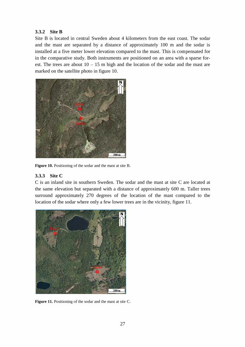
27

3.3.2 Site B

Site B is located in central Sweden about 4 kilometers from the east coast. The sodar

and the mast are separated by a distance of approximately 100 m and the sodar is

installed at a five meter lower elevation compared to the mast. This is compensated for

in the comparative study. Both instruments are positioned on an area with a sparse for-

est. The trees are about 10 – 15 m high and the location of the sodar and the mast are

marked on the satellite photo in figure 10.

Figure 10. Positioning of the sodar and the mast at site B.

3.3.3 Site C

C is an inland site in southern Sweden. The sodar and the mast at site C are located at

the same elevation but separated with a distance of approximately 600 m. Taller trees

surround approximately 270 degrees of the location of the mast compared to the

location of the sodar where only a few lower trees are in the vicinity, figure 11.

Figure 11. Positioning of the sodar and the mast at site C.

28

3.3.4 Site D

Site D is located about 15 kilometers south west of the town Söderhamn. There is no

sodar at the site but the mast which is positioned in a forested area at the top of a

mountain has been used in the long-term correction study.

29

4 RESULTS

This chapter presents the results from both the sodar and mast comparison and the long

term correction study. There will also be some short explanations in order to make the

results easier to comprehend.

4.1 COMPARISON OF SODAR AND MAST MEASUREMENTS

Table 2 presents the measuring period for each site.

Table 2 Measuring period for each site

Site Measuring period

A 03-Sep-2009 to 19-Sep-2009 0.6 months

B 17-Jun-2009 to 08-Aug-2009 1.7 months

C 26-May-2009 to 05-Oct-2009 3.4 months

Since the mast and the sodar at site C are located rather far from each other, see section

3.3.3, the most important studies are those carried out at site A and site B.

Required data to perform the data availability study was only available at site B and site

C. Figure 12 and figure 13 presents the data availability at site B and site C.

Figure 12. Sodar data availability for different measurement hights at site B.

0,90

0,91

0,92

0,93

0,94

0,95

0,96

0,97

0,98

0,99

20 30 40 50 60 70 80 90 100 110 120 130 140 150

Data

avail

ab

ilit

y [

%]

Measurement height [m]

Jättendal

30

Figure 13. Sodar data availability for different measurement hights at site C.

The sodar at site C has a better data availability compared to the sodar at site B. Besides

the expected loss in availability at the top of the wind profile, both sites have a small

lack in availability around 80 m height. There is also a lower availability at the bottom

of the wind profile compared to the middle of the profile at site B.

4.1.1 Mean wind speed and wind direction

The mean wind speed, mean difference and standard deviation for the three sites are

presented in table 3, table 4 and table 5. The mean difference is calculated by subtract-

ing sodar data from cup anemometer data.

Table 3 Mean wind speed, mean difference and standard deviation at site A

80 m 120 m

Mean wind speed sodar [m/s] 6.198 7.057

Mean wind speed mast [m/s] 6.110 7.015

Mean difference [m/s] -0.099 -0.030

Standard deviation [m/s] 0.589 0.636

0,90

0,91

0,92

0,93

0,94

0,95

0,96

0,97

0,98

0,99

20 30 40 50 60 70 80 90 100 110 120 130 140 150

Data

avail

ab

ilit

y [

%]

Measurement height [m]

Sävsjö

31

Table 4 Mean wind speed, mean difference and standard deviation at site B

a) Corrected for overspeeding

40 m 60 m 80 m 81.5 m 81.5m a)

Mean wind speed sodar

[m/s] 3.790 4.314 4.703 4.703

Mean wind speed mast

[m/s] 3.771 4.223 4.645 4.701 4.698

Mean difference [m/s] -0.019 -0.091 -0.058 -0.001 -0.006

Standard deviation [m/s] 0.655 0.596 0.628 0.649 0.650

Table 5 Mean wind speed, mean difference and standard deviation at site C

a) Corrected for overspeeding

40 m 60 m 80 m 81.5 m 81.5m a)

Mean wind speed sodar

[m/s] 4.362 5.237 5.93 5.926

Mean wind speed mast

[m/s] 4.171 4.864 5.57 5.631 5.625

Mean difference [m/s] -0.191 -0.372 -0.359 -0.295 -0.303

Standard deviation [m/s] 0.842 0.792 0.818 0.809 0.810

The mean wind speed measured by the sodar and the cup anemometers show a good

conformity for site A and site B. At site C there is a greater difference in mean wind

speed. The standard deviations do not show any clear significant dependence of

measuring height and are rather constant at each site. Site A and site B is within the

same magnitude of standard deviation.

The effect of overspeeding has been reduced on cup anemometer data for the top meas-

uring height at site B and site C. Site A lacked necessary data to perform the

calculation. According to table 4 and table 5 only a small reduction in cup anemometer

mean wind speed and no significant change in standard deviation were obtained.

Analyses of the wind direction are only performed at the heights where the mast has a

wind vane deployed and not at site A where data about wind direction was available.

Since the wind direction has a value between 1 to 360 degrees, problems may occur

when calculating the mean difference and standard deviation. When the sodar for

example reports a direction of 360 degrees, the wind vane may report a direction of 1

degree. This is a good conformity in wind direction but will introduce an error in case of

mean difference and standard deviation. Therefore, 360 degrees was added to the lowest

wind direction value when the difference in wind direction between the sodar and the

32

wind vane was larger than 250 degrees. This implies that the wind vane from the

example earlier has a value of 361 degrees which results in a difference of 1 degree

instead of 359 degrees.

Table 6 and table 7 presents the mean difference and the standard deviation where the

sodar wind direction is subtracted from the mast wind direction.

Table 6 Mean difference and standard deviation of wind direction at site B

40 m 80 m

Mean difference [°] 1.363 -2.855

Standard deviation [°] 18.92 16.68

Table 7 Mean difference and standard deviation of wind direction at site C

40 m 80 m

Mean difference [°] -3.781 -9.936

Standard deviation [°] 21.82 18.69

There was a smaller mean difference and standard deviation at site B compared to site

C. The sodar measures higher wind directions at site C and at 80 m height at site B.

4.1.2 Correlation study

Figure 14, figure 15 and figure 16 present the wind speed correlation between the sodar

and the cup anemometers at site A, site B and site C respectively. The data in the scatter

plots are ten minute averages reported by the sodar and the cup anemometers

Figure 14. Correlation of wind speed at site A.

33

Figure 15. Correlation of wind speed at site B.

34

Figure 16. Correlation of wind speed at site C.

The coefficient of correlation is increasing with altitude, except for the 81.5 m

measurement height at B where the value is almost the same as for 80 m. The best

correlation is achieved at site A but the correlation for site B is also quite good. The

correlation at site C is not as good as the other sites. Using an equation not allowing any

offset, i.e. , only gave a negligible difference in the coefficient of correlation.

When compensating for the overspeeding error at 81.5 m measuring height at site B and

site C there is no change in the coefficient of correlation.

Measurements below 5 m/s at site B seems to differ more compared to higher wind

speeds. Since measurements below 4 m/s are under the normal cut-in speed of a turbine,

they do not affect the energy yield calculation and were therefore excluded at 81.5 m to

see if the correlation improved. The result of doing this however was a lower coefficient

of correlation 0.913 instead of 0.941. The mean deviation was increased to -0.213 m/s

from -0.001 m/s, but the standard deviation did not change significantly. Since the mast

measures higher wind speeds compared to the sodar below 5 m/s, a possible explanation

for the differences might be overspeeding of the cup anemometers. Therefore, the

correlation at 81.5 m was calculated for the wind speeds between 0 – 5 m/s both when

the cup anemometer data was compensated and when it was not compensated for the

35

overspeeding error. The results showed no significant difference in correlation or in

mean wind speed and standard deviation.

The wind direction correlation study is performed with wind direction data that is not

compensated for the problem around zero degrees. No coefficient of correlation was

therefore calculated. However, the shape of the chart indicates the correlation between

the two instruments, figure 17 and figure 18.

Figure 17. Correlation of wind direction at site B.

Figure 18. Correlation of wind direction at site C.

The measurements are less scattered in figure 17 than in figure 18, which signifies a

better correlation of wind direction at site B than at site C. The problems around zero

degrees are displayed in the upper left and the lower right corner of each plot.

Turbulence intensity data were only available at site B and site C. Correlation analyses

are performed at 40 and 81.5 m measuring height and presented in figure 19 and figure

20.

36

Figure 19. Correlation of turbulence intensity at site B.

Figure 20. Correlation of turbulence intensity at site C.

There is a very low coefficient of correlation at both sites. The reason for an extremely

low correlation at site B is a number of outliers from the sodar not within the range of

the plot. Since the turbulence intensity is the ratio between the wind speed standard

deviation and the mean wind speed, low values of mean wind speed will result in high

turbulence intensities. The turbulence intensity values with a mean wind speed below 4

m/s were therefore rejected to study if the correlation improved. At site B the coefficient

correlation improved to 0.38 at 40 m height and to 0.22 at 81.5 m height. Corresponding

results for site C was 0.11 at 40 m height and 0.32 at 81.5 m height. This is still a low

coefficient of correlation. The result from both before and after the rejection of data

indicates that the sodar measures a lower turbulence intensity compared to the cup

anemometers.

4.1.3 Scalar and vector averaging

By studying the scatter plots from site B it is noticeable that the sodar has a tendency to

measure lower wind speeds below 5 m/s compared to the cup anemometers. One of the

reasons for that might be the differences between scalar and vector averaging of wind

data as discussed in section 2.4.1. This was studied at height 40 and 80 m, figure 21 and

figure 22.

37

Figure 21. Vector and scalar averaged wind speed, i.e. sodar and cup anemometer wind speed together

with the standard deviation of wind direction at 40 m height at site B.

Figure 22. Vector and scalar averaged wind speed, i.e. sodar and cup anemometer wind speed together

with the standard deviation of wind direction at 80 m height at site B.

There are some results supporting the theory that the sodar should report a lower wind

speed when there is a higher standard deviation of the wind direction, especially at 40 m

height around sample number 230 where the standard deviation is high. However, there

is no distinct trend in these measurements that indicates that the different averaging

0

10

20

30

40

50

60

0

1

2

3

4

5

Sta

nd

ard

dev

iati

on

[]

Win

d s

pee

d [

m/s

]

Sample number

40 m

Sodar Cup anemometer Std.dev. Dir

0

10

20

30

40

50

60

0

1

2

3

4

5

Sta

nd

ard

dev

iati

on

[]

Win

d s

pee

d [

m/s

]

Sample number

80 m

Sodar Cup anemometer Std.dev. Dir.

38

methods are the reason for the somewhat lower wind speed measured by the sodar

below 5 m/s.

4.2 LONG-TERM CORRECTION

The result of the long term correction study is presented in figure 23. A mean and medi-

an value of all the coefficients of correlation for a specific measurement period has been

calculated in order to prevent any seasonal impact on the result.

Figure 23. Mean and median value of the coefficients of correlation depending on the length of measure-

ment period.

Figure 23 shows that the largest increase in the coefficient of correlation occurs during

the first four months. The increase in correlation between the measurement period of six

months and seven months is smaller compared to the general trend for adjacent mea-

surement periods. The difference between the mean and the median values are only

significant during the shorter periods since extreme values are more common there.

0,70

0,75

0,80

0,85

0,90

0,95

1,00

1 2 3 4 5 6 7 8 9 10 11

Coef

icci

ent

of

corr

elati

on

Number of months

Mean

Median

39

The result from the study of seasonal impact on the correlation is presented in figure 24.

The x-axis represents the middle month in each measurement period, e.g. 3 means that

March is the middle month in all five series.

Figure 24. Seasonal impact on correlation for measurement periods of various lengths.

According to figure 24 there is a trend in the three shortest series that indicates a higher

coefficient of correlation during spring and autumn compared to summer and winter.

There is also a slightly better correlation during the autumn compared to the spring. The

two longest series do not show any distinct trend.

0,8

0,82

0,84

0,86

0,88

0,9

0,92

0,94

0,96

0,98

1

1 2 3 4 5 6 7 8 9 10 11 12

Coef

fici

ent

of

corr

elati

on

Month in center of measurement period

3 months

5 months

7 months

9 months

11 months

40

5 DISCUSSION

As this thesis is divided in to two parts, these parts will also be treated separately in the

discussion chapter.

5.1 COMPARISON OF SODAR AND MAST MEASUREMENTS

Information about the presence of fixed echoes, background noise and the attenuation of

sodar data at the top of the wind profile was obtained from the study of the sodar data

availability. Two reasons for better sodar data availability at site C compared to site B

might be that there are more fixed echoes and background noise present at site B. The

loss of availability in the lower parts of the wind profile at site B was probably due to

fixed echoes. However, no explanation was found for the small lack in availability

around 80 m height at both sites.

5.1.1 Wind speed

With respect to the distance between the instruments at the test sites, conclusions should

only be drawn from measurements at site A and site B. Measurements from these sites

indicated a good agreement between the sodar and the cup anemometer wind speed

measurements. The mean difference in mean wind speed at all heights was less than 0.1

m/s, which is equal to or below the accuracy of the sodar and the cup anemometer re-

spectively. There was a relatively big difference in measured wind speed (1.2%) be-

tween the cup anemometer at 80 and 81.5 m height at site B and the reason for that

might be that the anemometer at 81.5 m was top mounted and thereby less disturbed by

the mast structure.

According to this study the sodar measured a higher mean wind speed compared to the

mast at all sites. This was in contrary to both the theory and previous studies. The

reason for this was difficult to determine. However, the previous studies have been

carried out at one site each whilst this study was performed at three sites, indicating that

the sodar may measure higher wind speeds as well.

The differences in reported wind speed by the sodar and the mast below 5 m/s at site B

could not be explained by the overspeeding of the cup anemometer. Nor was it possible

to entirely explain the differences with the results from the study of scalar and vector

averaging. However, to make a proper study about the differences in wind speed

between scalar and vector averaging, it is necessary to have a software in the mast or the

sodar logger that reports both scalar and vector averaged wind speed. Otherwise, the

distance between the two instruments has an impact on the results. The vector averaged

wind speed may be more relevant in terms of energy yield calculations since the turbine

cannot respond to fast fluctuations in wind direction. A more detailed study of the

differences in wind speed between scalar and vector averaging would be an interesting

subject for further studies.

5.1.2 Wind direction

In terms of wind direction, it was only possible to evaluate the results from the compari-

son at site B since the distance between the sodar and the mast at site C was too far and

41

because there were no data from site A. According to the results from the study at site B

there was a good conformity in wind direction between the sodar and the wind vane. It

was not possible to conclude that one of the instruments measured higher or lower

values of wind direction compared to the other instrument since the wind vane

measured higher values at 40 m and the sodar measured higher values at 80 m height.

There was a smaller mean difference at 40 m height but a higher standard deviation

compared to 80 m height. This implies more extreme values in wind direction

differences at 40 m height which might be due to a higher degree of turbulence at lower

heights.

5.1.3 Turbulence

Since the comparison of turbulence measurements in this thesis were not detailed enou-

gh, no certain conclusions could be drawn. However, as expected from the theory it was

possible to determine that the sodar measured lower turbulence intensities compared to

the mast. This lower value should not be interpreted as incorrect since the cup

anemometer provides the value for turbulence intensity on a small scale and the sodar

reports turbulence intensity measured on a larger scale. It is a matter of what is desired

and at least for the time being turbulence measurements performed by a sodar are not

valid for the IEC WT 01 classification discussed in section 2.2. The result from the

turbulence study in this thesis indicated a significantly lower coefficient of correlation

compared to three non public previous studies (Bergström, pers.coum. 2010). However,

the result from the turbulence study carried out by Vattenfall showed resemblance with

the results in this study (Gustafsson, 2008). A more detailed turbulence comparison

study is of interest for further work.

5.1.4 Aspects not related to measuring technique

All measurements in this were been carried out during the summer and the autumn

which eliminates the possibility of under speeding by the cup anemometers due to icing

of the cups and freezing of the bearings. This implies reliable data, but to be able to

make a more thorough study it would be desirable to compare sodar and cup anemo-

meter data during the winter time as well. A source of error in this type of study was the

distance between the two instruments, but since it is impossible to have them located on

the same spot because of fixed echoes and wind wakes due to the mast structure, it

cannot be completely eliminated.

In terms of output data from the two instruments the sodar reports a wind profile for the

whole sweep area, whilst the mast usually only have a measurement at hub height and

one or maybe two at the lower part of the sweep area. A wind profile for the whole

sweep area enables a better estimation of the energy yield and provides more informa-

tion about the wind shear. As rotors are growing in size this becomes more and more

important. The towers are also growing in height which demands higher and thereby

more expensive met masts.

The mobility of the sodar enables a faster deployment and the possibility to measure the

wind at different locations within the future wind park area. A sodar is also easy to use

42

at a new site, compared to the mast which in addition to a new building permit also

needs to be disassembled and erected once again. Therefore, it is possible to use the

sodar as screening instrument and measure the wind during a relatively short period of

time at a new site to get an idea if the site is good enough to continue working with.

Since the price is about the same for a sodar and a mast (80 m), the sodar will probably

be the more cost efficient alternative because no extra cost is added when using it at a

new site. A disadvantage of the sodar is the need for more maintenance in terms of

refueling the diesel tank during periods of insufficient sunlight.

Using a sodar will eliminate the problems of over- and under speeding by the cup ane-

mometers and the wake effect due to the mast. On the other hand, it is important to

make an adequate positioning of the sodar to reduce the influence of background noise

and fixed echoes. This limits in a sense the use of sodar, but on the other hand the

instrument is possible to use in remote areas with no infrastructure.

A problem for the time being is that measurements from a sodar alone are not bankable

or accepted by turbine suppliers. This implies that a mast needs to be used to acquire

valid wind measurements. Perhaps all the comparative studies of sodar and already

accepted wind measuring instruments will change that fact.

5.2 LONG-TERM CORRECTION

Since this study was only carried out at one site, the results must be seen as site specific

and may not be generally valid. However, the tendency in the results might very well be

valid for other sites as well. It must also be kept in mind that the loss of data totally

amounts to 40 days of measurements. This implies that the long-term corrected refe-

rence series based on 12 months of short-term measurements actually only consists of

about 10.7 months.

5.2.1 Correlation study

The result of the correlation study shows a better correlation with an increasing length

of measurement period. This was expected since adding months to the measurement

period will make it more similar to the reference period consisting of 12 months. What

was more interesting though was that the fastest increase in correlation occurred during

the first four months. After that, the result shows a smaller and smaller increase in

correlation for every month added, except for the measurement period consisting of

seven months. The reason for a slightly smaller increase in correlation between the

measurement period of six months and seven months compared to the general trend for

adjacent measurement periods has no explanation and could be a coincidence for the

specific data used. A reason for the rapid increase in correlation during the first four

months might be due to the fact that every month added made up for a greater part of

the total measurement period when the period was relatively short. The rapid increase in

correlation during short measurement periods might also be due to the fact that lost or

rejected data has a greater impact on a shorter measurement period.

Since the correlation study was carried out between a long-term corrected measurement

series based on 12 months of short-term data and long-term corrected measurement

43

series based on fewer months of short-term data, the results are an indication on how

good a long-term correction with a shorter measurement period as short-term data repre-

sented a long-term correction based on a whole year of measurements. It is important

not to confuse that with the correlation between the concurrent data of a long-term

corrected measurement series and the original site measurement series, which has not

been studied in this thesis but is a common comparison. Another important thing to

keep in mind is that there are still uncertainties in the results even after a year of

measurements (Bergström & Nilsson, 2009).

5.2.2 Seasonal impact on the correlation

From the study on seasonal impact on the correlation it is evident that wind measure-

ments during the spring and the autumn represented a whole year of measurements

better than wind measurements performed during the summer and the winter. It is

difficult to explain this tendency but one possible reason might be the daily variations in

atmospheric thermal stability discussed in section 2.1.2. During the winter the nights are

longer than the days and there is a low heating of the ground. This implies a mostly

stable atmospheric thermal stability. Opposite conditions occur during the summer,

which means that an unstable stability dominates. The bias in atmospheric thermal

stability might be a reason for the lower correlation compared to spring and autumn

where the day and night are of a more equal length and both types of stability are

common. This theory is supported by an article in the DEWI Magazin in which a

similar study with analogous results was carried out (Borget et al., 2007).

The difference in correlation between the winter and the summer was larger for the

measurement period consisting of three months compared to the other measurement

periods. This might be due to the loss of data which only occurs during the winter and

has a greater impact on short measurement periods compared to longer periods. Conse-

quently, there were fewer measurements to base the long-term correction calculation on

during the winter.

The seasonal impact decreases with increasing length of measurement period because

longer periods contained more than one season. It should be kept in mind that this study

does not present the time of year with the highest wind speeds, but the time of year with

the most representative wind climate for a whole year.

44

6 CONCLUSIONS

From the comparative study of sodar and cup anemometer measurements it is possible

to draw the conclusion that the measurements performed by the AQ 500 Wind Finder

sodar are as valid as those performed by the cup anemometer and the wind vane.

Considering other aspects such as mobility, no need for permits, cost efficiency and the

fact that the sodar presents a vertical wind profile the sodar is the preferred choice.

However, if the aim is to perform long term wind measurements at a certain site a mast

might be more suitable due to its low demand for maintenance, unless heating of the

anemometers is required. Measurements performed by cup anemometers and wind

vanes are also bankable and accepted by the turbine suppliers.

The long-term correction study shows a large increase in correlation during the first four

months of measurements. It is therefore important to measure the wind for at least four

months in order to get a result from the long-term correction that somewhat represents

the result for a whole year of measurements.

It has been shown that there is a seasonal impact on the correlation. This impact

becomes less important with an increasing length of the measurement period but is

evident up to a measuring period of seven months. The tendency is a better correlation

during the spring and the autumn compared to the summer and the winter.

The overall conclusion of this thesis is that the sodar measurements are equivalent to

those obtained by a cup anemometer and that at least four months of measurements are

needed in order to perform an early evaluation of the long-term wind climate. It is also

concluded that measurements performed during the spring and the autumn represents

the wind climate for a whole year better than measurements carried out during the

summer and the winter.

45

BIBLIOGRAPHY

Antoniou, I., Courtney, M., Jørgensen, H. E., Mikkelsen, T., Hunerbein, S. v., Bradley,

S., Piper, B., Harris, M., Marti, I., Aristu, M,. Foussekis, D., & Nielsen, M. P. (2007).

Remote sensing the wind using Lidars and Sodars. Roskilde: Risø National Laboratory.

Antoniou, I., Jørgensen, H. E., Ormel, F., Bradley, S., Hünerbein, S. v., Emeis, S., &

Warmbier, G. (2003). On the Theory of SODAR Measurement. Roskilde: Risø National

Laboratory.

AQSystem. (2009). AQ500 Wind Finder - A remote sensing instrument for accurate

measurement of wind and turbulence. Tyresö, Sweden.

AQSystem. (2008). Wind Finder AQ 500 Operator Manual. Stockholm: AQSystem.

Bergström, H. (2008). Minutes of comparison between mast sensors and sodar.

Uppsala: Uppsala Universitet.

Bergström, H., & Nilsson, E. (2009). Från mätt vind till vindklimat -

Normalårskorrigering. Stockholm: Elforsk.

Berlin.de. (2007, January 31). Berlin.de. Retrieved February 6, 2010, from

http://www.stadtentwicklung.berlin.de/umwelt/umweltatlas/e_abb/ea403e01.gif

Borget, V., Monnier, P. A., & Strack, M. (2007, February). Long-term Scaling of Site

Measurements: Evaluation of Long-Term Meteorological Data in France and

Comparison of Correlation Methods. Dewi Magazin , pp. 61-68.

Bradley, S. (2008). Atmospheric acoustic remote sensing. Boca Raton: CRC Press.

Clive, P. J. (2008). Compensation of Vector and Volume Averaging Bias in Lidar Wind

Speed Measurements. Glasgow: IOP Publishing.

Danish Wind Indunstry Association. (2004, May 25). Roughness and shear. Retrieved

October 23, 2009, from www.windpower.org:

http://www.talentfactory.dk/en/tour/wres/shear.htm

ECMWF. (2008, January 23). ERA Project. Retrieved February 5, 2010, from ECMWF:

http://www.ecmwf.int/research/era/do/get/index

EMD International A/S. (2008). WindPRO 2.6 User Guide. Ålborg: EMD International

A/S.

Emd. (2010). WindPRO. Retrieved January 23, 2010, from EMD International A/S:

http://www.emd.dk/WindPRO/Frontpage

Energimyndigheten. (2007). Vindkraft - Bygga och ansluta större vindkraftverk.

Eskilstuna: Energimyndigheten.

46

Gustafsson, D. (2008). Remote wind speed sensing for site assessment and normal year

correction - The use of sodar technology, with special focus on forest conditions.

Department of Energy Technology. Stockholm: KTH.

Hunter, R. S. (Edited 2003). Recomended practices for wind turbine testing - 11. Wind

speed measurement and use of cup anemometry. Glasgow: Renewable Energy Systems

Ltd.

IEA RD&D Wind. (2007, Januari). Summary of IEA RD&D Wind – 51st Topical Expert

Meeting on State of the art of Remote Wind Speed Sensing. Retrieved October 30, 2009,

from IEA Wind:

http://www.ieawind.org/Task_11/TopicalExpert/09_07/51_Summary_Remote_Sensing

_TEM51.pdf

Manwell, J. F., McGowan, J. G., & Rogers, A. L. (2004). Wind Energy Explained -

Theory, Design and Applicatoin. Chichester: John Wiley & Sons Ltd.

National Center for Atmospheric Research . (2004, February 4). NCEP/NCAR

Reanalysis. Retrieved February 19, 2010, from MM5 Community Model:

http://www.mmm.ucar.edu/mm5/mm5v3/data/nnrp.html

Neal, B. D. (2008, May 24). About sodar. Retrieved December 7, 2009, from

Atmospheric Research & Technology - Sodar Home Page:

http://www.sodar.com/about_sodar.htm

Neal, B. D. (2009, August 27). Vector vs. Scalar Averaging. Retrieved November 19,

2009, from Atmospheric Research & Technology - Sodar Home Page:

http://www.sodar.com/VectorScalar.htm

Noord, M. d., Curves, A., Eecen, P., Antoniou, I., Jørgensen, H. E., Pedersen, T. F.,

Bradley, S,. Hünerbein, S. v., Kindler, D., Mellinghof, H., & Emeis, F. (2005). WISE -

WIND ENERGY SODAR EVALUATION FINAL REPORT. Netherlands: ECN.

NovaLynx Corporation. (n.d.). Glossary of Meteorological Terms. Retrieved November

11, 2009, from NovaLynx Corporation: http://www.novalynx.com/glossary-w.html

Poli, P. (2009). Reanalysis: Data assimilation aspects. Readign: ECMWF.

SMHI. (2008, August 8). Kunskapsbanken - Vind. Retrieved February 10, 2010, from

SMHI: http://www.smhi.se/kunskapsbanken/meteorologi/vind-1.362

Swedish Energy Agency. (2009, Januari 26). Wind power in Sweden. Retrieved October

19, 2009, from Energimyndigheten: http://www.energimyndigheten.se/en/About-

us/Mission/Wind-power-in-Sweden/

The Columbia Encyclopedia sixth edition. (2008). Encyclopedia.com - weather vane.

Retrieved November 10, 2009, from Encyclopedia.com:

http://www.encyclopedia.com/topic/weather_vane.aspx#1E1-weatherv

47

The European Wind Energy Assosiation. (2009, October 30). Regional Wind Resources.

Retrieved October 30, 2009, from Wind Energy - The Facts: http://www.wind-energy-

the-facts.org/en/part-i-technology/chapter-2-wind-resource-estimation/regional-wind-

resources.html

Theis Clima. (2009, Aprill 19). Wind Sensor - first class advanced. Retrieved Januari 4,

2010, from Theis Clima - The world of weather data:

http://www.thiesclima.com/windsensor_first_class_e.html

Thøgersen, M. L., Maurizio, M., Sørensen, T., & Nielsen, P. (2007). Measure-

Correlate-Predict Methods: Case Studies and Software Implementation. Aalborg: EMD

International A/S.

Totalförsvarets forskningsinstitut. (2006, March 28). Transport/Spridning. Retrieved

December 18, 2009, from Faktasamling CBRN:

http://www.faktasamlingcbrn.foi.se/filer/a_sidor/7/2.html

Vindforsk. (2009). Driftuppföljning av vindkraftverk, Årsrapport 2008. Stockholm:

Elforsk.

Westermann, D., & Rehfeldt, K. (2008). Summary of Cup Anemometer Classification.

Varel: Deutsche WindGuard Wind Tunnel Services GmbH.

Wilmers Messtechnik 2. (2003, July 21). Product information. Wind Direction Sensor

standard . Hamburg, Germany: Wilmers Messtechnik.

Wilmers Messtechnik. (2003, July 25). Product information. Cup Anemometer first

class . Hamburg, Germany: Wilmers Messtechnik.

Wizelius, T. (2007). Vindkraft i teori och praktiken. Lund: Studentlitteratur.

Wong, C. (2000). Speed of Sound in Air. Retrieved December 7, 2009, from The

Physics Factbook: http://hypertextbook.com/facts/2000/CheukWong.shtml

PERSONAL COMMUNICATIONS

Baurne, Kristian. (2009, December 14). Project Engineer. Nordex Sverige AB.

Bergström, Hans. (2010, February 6). Phd Meteorology. Uppsala Universitet.

Gross, Frank. (2010, February 16). Wind and site assesment, Nordex Energy GmBH.

Hurtig, Mats. (2009, December 2). Chairman of the Board. AQSystem.

Sondell, Niklas. (2010, February 19). Developer and Market Manager Sweden. Storm

Weather Center.

48

APPENDIX I

Table 1 presents the data that was lost in the long-term correction study due to an out of

order logger and freezing of the cup anemometer.

Table 1 The dates that were lost in the long-term correction study

Reason for loss Date

Out of order logger 20-Nov-2008 - 14-Dec-2008

Freezing of the cup anemometer 23-Jan-2009 - 02-Feb-2009

Freezing of the cup anemometer 05-Mar-2009 - 09-Mar-2009