the stability likelihood of an international climate

VU Research Portal

The stability likelihood of an international climate agreement

Dellink, Rob; Finus, Michael; Olieman, Niels

published inEnvironmental and Resource Economics2007

document versionPublisher's PDF, also known as Version of record

Link to publication in VU Research Portal

citation for published version (APA)Dellink, R., Finus, M., & Olieman, N. (2007). The stability likelihood of an international climate agreement.Environmental and Resource Economics.

General rightsCopyright and moral rights for the publications made accessible in the public portal are retained by the authors and/or other copyright ownersand it is a condition of accessing publications that users recognise and abide by the legal requirements associated with these rights.

• Users may download and print one copy of any publication from the public portal for the purpose of private study or research. • You may not further distribute the material or use it for any profit-making activity or commercial gain • You may freely distribute the URL identifying the publication in the public portal ?

Take down policyIf you believe that this document breaches copyright please contact us providing details, and we will remove access to the work immediatelyand investigate your claim.

E-mail address:[email protected]

Download date: 21. Feb. 2022

https://research.vu.nl/en/publications/a95c1468-98b7-4b88-a617-d6968750b4fe

Environ Resource EconDOI 10.1007/s10640-007-9130-7

The stability likelihood of an international climateagreement

Rob Dellink · Michael Finus · Niels Olieman

Received:15 February 2006/Accepted: 19 April 2007© Springer Science+Business Media B.V. 2007

Abstract Results derived from empirical analyses on the stability of climate coalitions areusually very sensitive to the large uncertainties associated with the benefits and costs of cli-mate policies. This paper provides the methodology of Stability Likelihood (SL) that linksuncertainties about benefits and costs of climate change to the stability of coalitions. We showthat the concept of SL improves upon the robustness and interpretation of stability analyses.Moreover, our numerical application qualifies conclusions from a recent strand of literaturebased on stylised models with ex-ante symmetric players that learning has a negative impacton the success of coalition formation in context of uncertainty.

Keywords Climate change modelling · International environmental agreements ·Non-cooperative game theory · Uncertainty

JEL Classification C79 · H87 · Q54

R. Dellink (B)Environmental Economics and Natural Resources Group, Wageningen University, Hollandseweg 1,Wageningen 6706 KN, The Netherlandse-mail: [email protected]

R. DellinkInstitute for Environmental Studies, Vrije Universiteit Amsterdam, Amsterdam, The Netherlands

M. FinusInstitute of Economic Theory, Department of Economics, University of Hagen, Hagen, The Netherlands

N. OliemanOperations Research and Logistics Group, Wageningen University, Wageningen, The Netherlands

N. OliemanRisk Model Validation and Methodologies Department, Rabobank Netherlands, Rabobank,The Netherlands

123

R. Dellink et al.

1 Introduction

There are many obstacles that prevent the formation of effective international environmentalagreements (IEAs). Two of the most important obstacles are free-riding and uncertainty.

First, IEAs aim at providing a public good and therefore countries face free-rider incen-tives. Typically it is beneficial for a country when other regions increase their abatementefforts. This free-riding problem has been studied extensively in theoretical models, as forinstance in Hoel (1992), Carraro and Siniscalco (1993) and Barrett (1994) and in empiricalclimate models, as for instance in Bosello et al. (2003), Botteon and Carraro (1997), Tol(2001), Eyckmans and Finus (2006), and Finus et al. (2006). A main conclusion of this lit-erature is that stable coalitions improve only marginally upon the non-cooperative outcomebecause either stable coalitions are small or the global abatement level that can be sustainedin larger coalitions is very low. However, regardless of the specific model, all of these papersdetermine stable coalitions in a deterministic setting.

Second, the uncertainties surrounding the future impacts of climate change as well asabatement costs are large. In particular, the benefits from abatement that arise in the distantfuture are highly uncertain, but also future abatement costs are not fully known. These issuesare highlighted for instance in Roughgarden and Schneider (1999) and Tol (2002, 2005).Depending on the model specification and assumptions, uncertainty and learning may eithercall for laxer environmental standards today or imply that countries follow the precaution-ary principle by increasing their short-term abatement efforts (Kolstad 1996a, b; Ulph andMaddison 1997; Ulph and Ulph 1997). However, regardless of how uncertainty and learningis captured in these papers and what this means for optimal abatement strategies, successcan only be evaluated if free-rider incentives are also included in the analysis. This impliesthat models with a single global decision-maker cannot provide full insight into the regionalimpacts of uncertainty and learning. This drawback is common to most integrated assess-ment models that are used to analyse optimal abatement strategies, including for instanceDICE/RICE (Nordhaus and Boyer 2000), MERGE (Manne et al. 1995) and EPPA (Babikeret al. 2001). This also applies to some extent to models with two countries that comparenon-cooperative with cooperative behaviour and hence coalition formation is not really anissue in these models (e.g. Ulph and Maddison 1997; Ulph and Ulph 1997).

Recently, some papers have appeared that combine coalition formation with uncertaintyand learning (Na and Shin 1998; Ulph 2004; Kolstad and Ulph 2006; Kolstad 2007). Theyassume uncertainty about parameter values of the payoff function where probability distri-bution functions are known to all countries. In the context of coalition formation, in whichcountries choose their membership in the first stage and their abatement strategies in thesecond stage, this allows to distinguish three cases according to Kolstad and Ulph (2006)and Kolstad (2007): (1) Uncertainty is resolved before the first stage. This corresponds to thecase of full learning. (2) Uncertainty is resolved after the first stage but before the secondstage. This corresponds to the case of partial learning. (3) Uncertainty is not resolved. Thisis the case with no learning. In cases 1 and 2 where there is learning, it takes the form ofperfect learning, i.e. all players learn the true values of all uncertain parameters.

All these papers are stylized models with ex-ante identical players and mostly come tothe conclusion that learning has a negative impact on the success of coalition formation. Naand Shin (1998) compare case 2 and 3, but their model is essentially static (flow pollutant)and restricted to only three countries. The first restriction is removed in Ulph (2004), whocompares all three cases and considers a two period model with a stock pollutant. Due tothis complication, results are based on simulations and conclusions are not always clear-cut.Moreover, he assumes that countries have only two abatement strategies (no abatement versus

123


full abatement), the only uncertainty concerns the benefits from global abatement, with onlytwo states (low and high benefits) and uncertainty is correlated between players. This meansthat in the case of learning all countries are also ex-post identical; either all countries arelow or high benefit countries. These assumptions are also made in Kolstad (2007). Becauseof the assumption of a flow pollutant, he unambiguously shows that when comparing case 1and 3, learning increases the size of a stable IEA but has a negative impact on global welfare,as proven in Kolstad and Ulph (2006). Case 2 is ambiguous; learning may have a positive ornegative impact on participation and welfare. Finally, in the case of uncorrelated uncertainty,Kolstad and Ulph (2006) confirm the negative impact of learning, but again have to resort tosimulation, despite the assumption that all countries are ex-ante identical and that there areonly two states in the world.

Because of the difficulties of deriving analytical results even in a simple model, we con-sider uncertainty, learning and coalition formation based on an empirical climate model withtwelve heterogeneous world regions. In the first stage, regions can only choose betweenbecoming a signatory or to remain an outsider as assumed in the papers above. However, inthe second stage, regions can choose from a continuum of abatement strategies, while almostall model parameters are assumed to be uncertain with (uncorrelated) probability distributionfunctions. We restrict ourselves to the analysis of cases 1 and 3, namely no and full resolutionof uncertainty. Case 1 is relatively straightforward. Because we assume that utility is linearin payoffs as in Kolstad and Ulph (2006), we can also apply the certainty equivalence prin-ciple. That is, the case of no resolution of uncertainty is identical to the deterministic caseif the mean or expected value of a parameter corresponds to the value in the deterministiccase. Together with case 3, which is the focus of this analysis, case 1 allows for a directcomparison with the conclusions derived in Kolstad and Ulph (2006). Case 3 implies thata coalition cannot be called stable or not stable any longer (based on certain payoffs in thedeterministic case or expected payoffs in the case of no resolution of uncertainty). For this,we introduce our concept of Stability Likelihood (SL), which determines the likelihood thata coalition structure is stable. Compared to Kolstad and Ulph (2006) and the other papersabove, we find that learning does not always have a negative impact on the success of coalitionformation. Moreover, we show that the concept of SL has advantages over a deterministicanalysis. Firstly, in a deterministic setting, coalitions can only be stable or unstable. This mayimply in some cases that small perturbations of parameters are sufficient to change the set ofstable coalitions, invalidating conclusions. Secondly, in a deterministic model, uncertaintyof parameter values can only be indirectly accounted for through sensitivity analyses whereeach analysis is subject to the first problem mentioned above. Hence, the concept of SL canbe interpreted as a more sophisticated sensitivity analysis than is traditionally done in thecontext of coalition formation with empirical data, as for instance in Eyckmans and Finus(2006) and Finus et al. (2006).

In the following, we present our model of coalition formation and introduce the conceptof SL in Sect. 2. Section 3 discusses the calibration of the model, including the distributionfunctions used for the uncertain model parameters. Section 4 presents and discusses resultof our stability analysis. Section 5 concludes.

2 The model of coalition formation

Consider a set of N heterogeneous players, each representing a region of the world. In thefirst stage, regions decide whether to become a member of IEA or to remain an outsider.Announcement ci = 1 means “Region i joins the coalition” and announcement ci = 0

123

R. Dellink et al.

“Region i remains an outsider”; a coalition structure c is described by announcement vectorc = (c1, . . . , cN ). The set of players that announce 1 are coalition members and is denoted ask = {i | ci = 1, ∀i = 1, . . . ,N }. Thus, in this simple setting, a coalition structure is definedby coalition k. Hence, we can use the term coalition structure and coalition interchangeably.Note that there are 2N announcement vectors, but essentially there are only 2N − N coalitionstructures. The reason is that regardless whether all regions announce ci = 0 or only oneregion announces ci = 1 and all other announce ci = 0, this will result in the “All-SingletonsCoalition Structure”.

In the second stage, regions choose their abatement levels. This leads to abatement vectorq = (q1, . . . , qN). The payoff of an individual region i, πi (q, b) depends on abatement vec-tor q (and hence on the strategy of all regions, due to the public good nature of abatement)and on a vector of model parameters b.

We solve the game backwards assuming that strategies in each stage must form a Nashequilibrium. For the second stage, this entails that abatement strategies form a Nash equilib-rium between coalition k and the remaining non-signatories. That is,

∑

i∈k

πi (q∗k , q∗−k, b) ≥

∑

i∈k

πi (qk, q∗−k, b)∀qk and

πi (q∗k , q∗

i , q∗−i , b) ≥ πi (q∗k , qi , q∗−i , b)∀qi (1)

where qk is the abatement strategy vector of coalition k, q−k the vector of all regions notbelonging to k, qi the strategy of non-signatory i , and q−i the strategy vector of all othernon-signatories except i . An asterisk denotes equilibrium strategies. Computationally, thisimplies that non-signatories (i /∈ k) that announced ci = 0 will choose their abatement strat-egies so as to maximize their individual payoff πi (q, b), whereas all signatories (i ∈ k) thatannounced ci = 1 jointly maximize the aggregate payoff of their coalition

∑i∈k πi (q, b),

taking the abatement strategies of all other regions as given. Strategically, this means that thebehaviour of non-signatories towards all other regions is selfish and non-cooperative; signa-tories’ behaviour is cooperative towards their fellow members, but non-cooperative towardsoutsiders. Economically, this means strategies are group (but not globally) efficient withincoalition k. Hence, the equilibrium economic strategy vector q∗ corresponds to the classical“social or global optimum” if coalition k comprises all countries, i.e. the grand coalitionforms, and corresponds to the classical “Nash equilibrium” if coalition k comprises onlyone member or is empty. Thus, any inefficiency stems from the fact that k is not the grandcoalition.

Since in the context of our empirical model the equilibrium abatement vector q∗ is uniquefor every coalition structure c and a given vector of parameters b (see the proof in Olieman andHendrix 2006), there is a unique vector of equilibrium payoffs for every coalition structure c:

vi (c, b) ≡ πi (q∗(c), b).

We now turn to the first stage. Also in the first stage, strategies form a Nash equilibrium.That is, no signatory that announced ci = 1 should have an incentive to change its announce-ment to ci = 0 (internal stability) and no non-signatory that announced ci = 0 should wantto announce ci = 1 (external stability), given the announcement of other players c−i . Forour purposes, this condition can be summarised compactly by the payoff stability functionf (c, b), which assigns the value 1 to a stable announcement vector (i.e. stable coalition) andthe value 0 to an unstable announcement vector (i.e. unstable coalition):

123


f (c, b) =⎧⎨

⎩

1 if (vi (ci , c−i , b)− vi (ci , c−i , b) ≥ 0) for ci = 1 − ci and for alli = 1, . . . ,N

0 else(2)

The function f (c, b)will take on the value 1 if for all regions the payoff from announcementc is higher than, or equal to, the payoff associated with alternative announcements c. Thesealternatives are constructed by changing the announcement of one player at a time. It is worthnoting that for any given set of parameters b, this function allows for either a unique stablecoalition, multiple stable coalitions or no non-trivial stable coalition.

In a deterministic model, the vector of parameters b may be based on estimates but istreated as given. In contrast, in a stochastic model the deterministic vector of parameters bis replaced by the stochastic (vector) variable b which is characterised by probability space(B, B,Pr) and probability density function g (b). In the case of no resolution of uncertainty,the decision on membership in the first stage will be based on expected payoffs using themean values of b. If the vector of mean values of b is b, this corresponds to the deterministicsetting. However, in the case of full resolution, decisions are based on the stochastic variableb and as function f (c, b) becomes a Bernoulli variable, we can assign a likelihood to theevent f (c, b) = 1, i.e. to a stable coalition.

The SL of coalition structure c is therefore defined as SL ≡ Pr { f (c, b) = 1}, whichequals

∫B f (c, b) · g(b)db. Assuming that f (.) is a correct representation of reality, we can

interpret SL as the probability that coalition structure c is stable.The heterogeneity of players with payoff functions based on the empirical model STACO

(see Sect. 3), requires us to resort to numerical calculations for the SL of various coalitions.1

The SL is calculated using a Monte Carlo sampling technique: we generate M samples bm

from b; based on these samples we can estimate the SL with SL = 1M

∑Mm=1 f (c, bm) that

has an estimated variance of 1M−1

(SL

(1 − SL

)).

A more detailed discussion of the SL concept and computation methods can be found inOlieman and Hendrix (2006).

3 Calibration of the model

3.1 Introduction

In this section, the calibration of the empirical model, called STAbility of COalitions (STA-CO) is described. For more detailed information on the model and calibration procedure, seeDellink et al. (2004) and Finus et al. (2006). The model comprises benefit and cost functionsof twelve world regions: USA (USA), Japan (JPN), European Union (EEC), other OECDcountries (OOE), Eastern European countries (EET), former Soviet Union (FSU), energyexporting countries (EEX), China (CHN), India (IND), dynamic Asian economies (DAE),Brazil (BRA) and “rest of the world” (ROW). The philosophy behind the construction of themodel comprises two items. First, the model must be simple enough to allow for sufficientsamples to be calculated within reasonable time.2 Second, the model should reflect importantresults and features of integrated assessment models in terms of overall magnitudes of global

1 We are not aware of any paper that provides analytical solutions of stable coalitions in the context ofheterogeneous players even in the absence of uncertainty.2 We need around 40,000 samples to get sufficient accuracy in the estimates of SL. This implies around 2billion calculations of optimal regional abatement and payoff levels (40,000 times 12 regions times 4096membership announcement vectors).

123

R. Dellink et al.

emissions and concentration, abatement costs from regional abatement and benefits fromglobal abatement over some time period. Therefore, the model focuses on carbon dioxide,but the exogenous level of other greenhouse gases is included in the calibration of the benefitfunction (cf. Nordhaus 1994). The analysis is based on the net present value of a stream ofnet benefits starting in 2010 and covering a time period of 100 years in order to capture thelong-run effects of global warming. They are computed for every possible coalition structureand then stability is computed according to the procedure explained in Sect. 2. The pricefor this complexity (see footnote 2) is that we assume constant abatement strategies (cf.Sect. 3.2), rendering the model essentially static as in Na and Shin (1998), Kolstad and Ulph(2006) and Kolstad (2007). Therefore, numerical results should be interpreted with caution.However, this allows for a direct comparision with the papers mentioned above about the roleof learning. Moreover, we believe that our simulations illustrate the usefulness of SL as anindicator, as we include the best available information on the probability density functionsof the model parameters.

3.2 Elements of the empirical model

The payoff function of region i is given by:

πi =T∑

t=1

(1 + r)−t (Bit (qt )− ACit (qit )) (3a)

where T denotes the time horizon, t = 2011, . . . , 2110; r is the discount rate; Bit are ben-efits from global abatement (qt = ∑N

i=1 qit); and ACit are abatement costs from regionalabatement qit .

The payoff function is calculated as the net present value of a stream of net benefits fromabatement between 2010 and 2110 and thus reflects discounted avoided damages minus dis-counted abatement costs. Regional abatement costs are a function of the level of individualabatement by region i , while regional benefits depend on global abatement efforts.

Assuming constant abatement strategies (qit = qi/100), benefits in year t can be expressedas a function of global abatement over the entire period. Furthermore, we consider that thestock of CO2 can be approximated by a linear function of emissions and that damages arelinear in the stock of CO2.3 It follows that annual global benefits from reduced emissions arealso linear in the level of abatement:

Bt (q) = ϕt · q (4a)

where ϕt denotes marginal benefits in period t from total abatement over the entire period.This parameter also includes the effects of limited retention of GHGs in the atmosphere andthe decay of the stock of GHGs over time. As benefits in period t result from the stream ofabatement in all periods until t , these marginal benefits are increasing over time.

Discounted global or total benefits, T B(q) can then be expressed as

T B(q) = γ · q (4b)

where γ represents discounted marginal benefits in $/ton carbon equivalents (tC) and iscalculated as

γ =2110∑

t=2011

(1 + r)−t · ϕt . (5)

3 The details of this approximation are given in Dellink et al. (2004).

123


Regional discounted benefits are assumed to be a share of discounted global benefits fromabatement:

T Bi (q) = si · T B(q) = si · γ · q (4c)

where si is the share of global benefits for region i and∑N

i=1 si = 1.For the specification of the abatement cost functions, estimates of the EPPA model are

used (Ellerman and Decaux 1998). It assumes an annual abatement cost function of region iof the following form:

ACit (qit ) = 1

3· αi · (qit )

3 + 1

2· βi · (qit )

2 (6a)

with αi and βi regional cost parameters. Total abatement cost of region i, T ACi (qi ), is thesum of annual abatement cost over the entire time horizon. Assuming constant strategies anda constant discount rate, as in the case of benefits, the total abatement cost function becomes

T ACi (qi ) = ρ ·(

1

3· αi · (qi )

3 + 1

2· βi · (qi )

2)

(6b)

with

ρ =2110∑

t=2011

(1 + r)−t . (7)

Taken together, the payoff function of region i can be written as:4

πi = T Bi (q)− T ACi (qi ). (3b)

Generally, all model parameters are uncertain. However, we have insufficient informationto fully estimate the probability density functions of all parameters at a regional level. Amore advanced meta-analysis of published and unpublished estimates would require a studyof its own and therefore is beyond the scope of the current paper. Hence, we consider onlyuncertainty of the benefit and cost parameters γ, si , αi and βi . Other parameters, such asemissions in 2010, the decay rate of greenhouse gases and the discount rate are assumed tobe known with certainty. Calibration of emissions and concentrations is based on the widelyknown DICE-model by Nordhaus (1994).

The discount rate r is set at 2% per year. This is in line with Weitzman (1998, 2001) whosuggests that in the case of climate change long-terms effects should be discounted with alow discount rate and suggests that 2% is appropriate for the “medium future”. In Sect. 4.3,we also consider the possibility of a higher discount rate, though this done indirectly by low-ering the mean value of the global benefit parameter γ . We want to stress that the discountrate only affects the aggregation of costs and benefits over time, as marginal benefits are

4 This means that we base our stability analysis on the net present value of benefits and abatement costs (i.e.discounted payoffs). The assumption that the abatement paths are constant over time simplifies the calcula-tions, but is not essential. The nature of our analysis requires only that the overall magnitude of concentrationsand emissions mimics that of more elaborate integrated assessment models (because decisions whether tojoin a coalition are based on discounted payoffs). The exact shape of the equilibrium emission or abatementpaths are not important for our analysis. A similar stability analysis in a deterministic setting with dynamicequilibrium abatement paths, as reported in Nagashima et al. (2006), reveals that the impact of our simplifyingassumption is limited: while levels of payoffs are somewhat affected, the stability of coalitions is robust inthis respect.

123

R. Dellink et al.

Table 1 Characteristics of the2-sided exponential distributionfunction of the global benefitparameter γ

Value

5% Density −9 $/tC

Mode 5 $/tC

Density at mode 13%

95% density 245 $/tC

Mean 77 $/tC

constant (though uncertain). Note also that our assumption of a constant (money) discountrate is consistent with a low, but positive, pure rate of time preference.5

3.3 Global benefit function

The distribution function of the global benefit parameter γ is based on a recent study byTol (2005). The probability density function of peer-reviewed studies as presented by Tolcan be closely mimicked by a 2-sided exponential function. This function is described byfour pieces of information: (i) the 5 percentile point; (ii) the value where the two sides ofthe exponential function are separated (assuming this is above the 5 percentile point); (iii)the cumulative probability density at this separation value; and (iv) the 95 percentile point(assuming this is above the separation value). The first piece of information is given by thevalue that corresponds to a cumulative probability of 5%; this value equals −9 $/tC, implyinga strictly positive probability that benefits from abatement are negative. The point of separa-tion between both sides of the function is given by the mode and equals 5 $/tC; the associatedcumulative probability density is 13%. The point on the right side of the function is given bythe 95% cumulative probability density and equals 245 $/tC. The mean value of this functionis 77 $/tC. These numbers are summarised in Table 1 and the corresponding histogram ofall drawn samples is shown in Appendix I. This distribution function implies that there isa probability of around 9% that the benefits from global abatement are zero or negative. Inthis case, optimal abatement is zero, and regions are indifferent between no, partial and fullcooperation.

3.4 Regional benefit shares

The distribution function of regional benefit shares (si ) is based on insights from a study byTol (2002). However, this source does not provide sufficient information on the functionalform of the distribution function of these shares. Therefore, we opt for a gamma distributionthat can handle the lower bound of the shares such that no region receives a negative shareof the benefits. Moreover, as the shares can vary between zero and one and the mean valueis typically close to zero, the distribution function should be skewed, as this is the case for agamma distribution. However, the choice of the gamma distribution function will be subjectto a sensitivity analysis in Sect. 4.4.

The mean values used for the regional shares are the values reported in the deterministicsetting of the STACO model, which are in turn based on Fankhauser (1995) and Tol (1997).Standard deviations are based on expert judgement, using in particular Tol (2002). Typically,

5 Alternatively, we could assume a constant pure rate of time preference of 0.5% and use the Ramsey ruleto derive a declining discount rate; as only net present values matter in our model, these two alternatives areequivalent for our analysis.

123


Table 2 Characteristics of thegamma distribution function ofthe regional parameter si (shareof global benefits)

Region Lower bound Mean Standard deviation

USA 0 0.2263 0.1414

JPN 0 0.1725 0.1078

EEC 0 0.2360 0.1475

OOE 0 0.0345 0.0216

EET 0 0.0130 0.0130

FSU 0 0.0675 0.0675

EEX 0 0.0300 0.0300

CHN 0 0.0620 0.0620

IND 0 0.0500 0.1000

DAE 0 0.0249 0.0498

BRA 0 0.0153 0.0306

ROW 0 0.0680 0.1360

standard deviations are of the same order of magnitude as mean values, and are lower forOECD countries than for the other regions. The regional numbers are represented in Table 2.For a better understanding, the corresponding histograms for the USA and China are shownin Appendix I.

After the samples of the regional shares are drawn, all shares are scaled up or down toforce the sum of shares to unity. This implies that the regional shares do not strictly followthe gamma distribution and the resulting variance in the shares is smaller than in the originalgamma distribution.6 Though rescaling is not a necessary condition for the working of themodel, the restriction on the sum of shares is enforced to avoid an impact of variations inthis parameter on global benefits. The consequences of this assumption will be investigatedin a sensitivity analysis in Sect. 4.4

3.5 Abatement cost functions

The two regional abatement cost parameters (αi and βi ) cannot be assumed to be indepen-dent. Typically, empirical studies report only variations in marginal abatement costs withoutproviding information on how the slopes and curvatures of these functions vary. Therefore,we assume the functional form of the abatement cost curves to be given, and vary the levelof marginal abatement costs per region in the simulations. This implies that both parametersin the abatement cost functions move simultaneously and in the same direction.7

We assume a normal distribution function; the mean is based on the deterministic versionof the STACO model, which is in turn based on Ellerman and Decaux (1998). The normaldistribution is chosen, as a priori, there seems to be no reason to assume a skewed distribution.The standard deviation of the abatement cost parameters are based on information providedby IPCC (Metz et al. 2001). Due to lack of regional information, the standard deviation is

6 More information on the impact of this rescaling on the probability density function can be obtained fromthe authors upon request.7 Effectively, we replace equation (6b) by T ACi (qi ) = ψi · ρ ·

(13 · αi · (qi )

3 + 12 · βi · (qi )

2)

, where ψi

is stochastic with mean value 1 and αi and βi are deterministic. However, we interpret the model as if thevariation occurs in αi and βi .

123

R. Dellink et al.

Table 3 Characteristics of the normal distribution of the abatement cost parameters αi and βi

Region αi βi

Mean Standard deviation Mean Standard deviation

USA 0.00050 0.00006 0.00398 0.00050

JPN 0.01550 0.00194 0.18160 0.02270

EEC 0.00240 0.00030 0.01503 0.00188

OOE 0.00830 0.00104 0.00000 0.00000

EET 0.00790 0.00198 0.00486 0.00122

FSU 0.00230 0.00058 0.00042 0.00011

EEX 0.00320 0.00080 0.03029 0.00757

CHN 0.00007 0.00002 0.00239 0.00060

IND 0.00150 0.00038 0.00787 0.00197

DAE 0.00470 0.00118 0.03774 0.00944

BRA 0.56120 0.14030 0.84974 0.21244

ROW 0.00210 0.00053 0.00805 0.00201

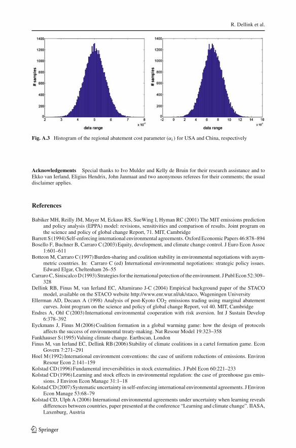
calibrated to 12.5 % of the mean for OECD regions and 25% for non-OECD regions. Hence,the variation in abatement costs is typically much smaller than the variation in benefits formost regions. The key inputs for the normal distribution are shown in Table 3 and for USAand China the corresponding probability density functions are illustrated in Appendix I.

4 Results

Using the confidence intervals and distribution functions described above, we calculate theSL of all possible 4084 coalition structures. Results of this simulation are reported and dis-cussed in Sect. 4.1. Section 4.2 identifies, which uncertainties are the main determinantsof the SL for selected coalitions using a meta-modelling approach. Section 4.3 investigatesan alternative scenario with lower probability of extreme observations for the benefits fromabatement, by adopting much stricter bounds on the distribution function of the global benefitparameter. These stricter bounds imply a lower mean value of global benefits. Section 4.4briefly discusses the results of some sensitivity analyses on the uncertainty of the variousparameters and the associated distribution functions. All simulations are carried out with aprecision of 95% on the second digit of SL (σSL = 0.0025), implying that we keep drawingsamples until we have sufficient accuracy on SL to present two decimals.

4.1 Results for the base specification

Table 4 presents the main results for those coalition structures that have the highest SL andfor the Grand Coalition. Note that the stability of the All-Singletons Coalition Structure isSL = 1 by definition. This coalition structure can always be supported as an equilibrium if allregions announce ci = 0. In the All-Singletons Coalition Structure abatement efforts amountto almost 70 GtC per century, or an annual abatement of 5.8% of global emissions in 2010,which leads to a discounted payoff of almost 8.8 trillion US$ over the century. The relativelyhigh abatement level is due to a high value of the global benefit parameter γ in the study

123


Table 4 Results for selected coalitions (mean values)

Coalition SL (fraction) Strict SL Total abatement Abatement Total(fraction) (GtC) (% of emissions) payoff (bln $)

All-Singletons 1 1 69.4 5.8% 8775

JPN,EEC 0.24 0.15 74.5 6.2% 9251

USA,JPN 0.15 0.06 79.1 6.6% 9663

USA,EEC 0.14 0.05 84.7 7.1% 10090

JPN,BRA 0.12 0.02 69.7 5.8% 8824

JPN,ROW 0.11 0.02 76.7 6.4% 9613

EEC,ROW 0.11 0.01 79.2 6.6% 9835

JPN,IND 0.10 0.01 78.0 6.5% 9773

JPN,FSU 0.10 0.01 75.8 6.3% 9475

EEC,BRA 0.10 0.01 70.1 5.9% 8857

EEC,FSU 0.10 0.01 78.4 6.6% 9699

Grand Coalition 0.09 0 326.3 27.3% 27360

of Tol (2005), as discussed in Sect. 3.3, and due to our assumption of a relatively moderatediscount rate. A major part of the global abatement effort is carried out by the two regionsthat have very flat marginal abatement cost curves, the USA and China. For these regions,equating marginal abatement costs to marginal benefits implies substantial abatement levels.In contrast, Brazil, which is characterised by a very steep marginal abatement cost curve andlow marginal benefits, hardly undertakes any abatement alone.

The relationship between the samples of global marginal benefits γ and the correspondingglobal abatement levels is illustrated in Fig. 1 for the All-Singletons Coalition Structure. Forsamples with negative marginal benefits, optimal global abatement is zero. For positive mar-ginal benefits, there is a clear positive correlation between the marginal benefits and globalabatement, but the relation is not linear. As marginal abatement costs increase quadratic inabatement, higher marginal benefits lead to a less than proportional increase in abatementlevels.

The graph clearly shows the dispersion of global marginal benefits as generated by thedistribution function and the resulting dispersion of optimal global abatement levels. The bulkof samples produces global marginal benefits between 0 and 200 $/tC, with correspondingoptimal global abatement of less than 200 GtC over the century, though outliers may havemarginal benefits of more than 800 $/tC, while global abatement may be as high as 400 GtC.

The Grand Coalition would lead to a much larger global abatement effort and a higherglobal payoff than no cooperation, as the gains from cooperation are fully reaped. However,the Grand Coalition has a low SL. Though it is externally stable by definition, the SL forinternal stability is very low. In fact, the Grand Coalition is only stable when there are nobenefits to be reaped from abatement, i.e. when the global benefit parameter γ is zero ornegative. In such cases, optimal abatement levels are zero, and hence regions have no incen-tive to leave this coalition. In the calculation of SL, this is interpreted as stable. Therefore,Table 4 also reports “Strict SL”, which equals SL minus the “probability of indifference”.

Only a few non-trivial coalitions (i.e. coalitions with at least two members) have a positivestrict SL. All these coalitions are small and improve only little over the All-Singletons Coa-lition Structure. The coalition of Japan and the European Union (EEC) has the highest SL.

123

R. Dellink et al.

0

50

100

150

200

250

300

-100 -50 0 50 100

150

200

250

300

350

400

450

500

Global marginal benefits ($/tC)

Glo

bal

abat

emen

t(G

tC)

Fig. 1 Relationship between global marginal benefits and global abatement levels in the All-singletons coa-lition structure

Therefore, we have a closer look at this coalition in Table 5, which provides regional data.Though the standard deviations of the abatement levels are rather high, there is a probabil-ity of more than 90% that abatement levels are strictly positive, implying that the implicitdistribution function for abatement levels is right-skewed. Though they are not part of thecoalition, the largest abatement efforts are carried out by China and the USA. These regionshave strong incentives to unilaterally reduce their emissions because of flat marginal abate-ment cost functions compared to their high constant marginal benefits.8 For Japan and theEuropean Union, marginal abatement costs are equal to the sum of marginal benefits ofthis coalition, reflecting the first order condition implied by the assumption of joint welfaremaximisation of coalitions as explained in Section 2.9

The last column in Table 5 shows the mean incentive to change membership. For exam-ple, if the USA were to join the coalition of Japan and European Union, its mean payoffwould be reduced by 247 bln $. Similarly, Japan and the European Union would have a lowerpayoff of 79 and 12 bln $, respectively, if they were to leave the coalition. It turns out thatthe mean values for the incentive to change membership are negative for all regions. Thus,a deterministic model assuming mean parameter values, would come to the conclusion thatthis coalition is stable. However, the corresponding SL is only 24%, implying that in threequarter of all samples the coalition is unstable. This clearly illustrates the importance of usinga more sophisticated stability indicator, such as SL, when the probability density functionsof the model parameters are strongly skewed. Moreover, in a deterministic setting, no othercoalition would be stable, even though there are some other coalitions with a positive SL.

8 This is in line with the arguments put forward by the Bush administration: the USA will not ratify the Kyotoprotocol, but will carry out abatement efforts in its own interest.9 For singletons, the equality between regional marginal abatement costs and regional marginal benefits holdsfor every sample if marginal benefits are non-negative. However, this must not necessarily hold for meanvalues. Similarly, for coalition members regional marginal abatement costs equal the sum of marginal benefitsof coalition members at the level of individual samples, but not necessarily for mean values.

123


Table 5 Regional results of the coalition Japan (JPN) and the European Union (EEC)

Region Total abatement Abatement Total payoff MACi ($/tC) MBi ($/tC) Incentive(GtC) (% emission) (bln $) (bln $)

Mean Standard Mean Mean Standard Mean Mean Meandeviation deviation

USA 20.31 16.01 8.4% 2050 4313 17.6 17.3 −247

JPN 2.83 2.68 5.1% 1650 3525 31.7 13.3 −79

EEC 12.29 9.15 8.8% 2043 4213 31.7 17.9 −12

OOE 2.30 1.71 3.7% 369 817 2.9 2.8 −127

EET 1.14 1.20 2.2% 141 406 1.1 1.1 −145

FSU 5.64 5.11 5.6% 670 1712 5.4 5.3 −221

EEX 1.40 2.01 1.2% 312 850 2.5 2.4 −206

CHN 21.02 24.19 8.9% 611 1739 4.9 4.8 −1282

IND 3.30 5.59 5.2% 441 1647 3.6 3.5 −289

DAE 0.81 1.80 2.0% 245 1008 1.9 1.9 −167

BRA 0.03 0.08 0.2% 151 636 1.2 1.2 −11

ROW 3.42 5.54 4.9% 568 2117 4.7 4.6 −227

Note: MACi = regional marginal abatement costs; MBi = regional marginal benefits, Incentive = change in netbenefits if one region changes its announcement of membership, given the announcement of all other regionswhere initially all regions anncounce ci = 0, except JPN and EEC that announce ci = 1

As discussed in the introduction, we can also relate our results to the cases of no and fulllearning in the presence of uncertainty (i.e. no and full resolution of uncertainty) as describedin Kolstad and Ulph (2006). The case of no learning corresponds to the deterministic set-ting. Hence, the expected total payoff in case of no learning is 9251 bln $, resulting from theonly stable coalition between Japan and the European Union. In the case of full learning,the expected payoff is the average payoff of all stable coalitions for each parameter sample.It seems plausible to assume that if there are multiple stable coalitions for a sample, eachequilibrium is equally likely. It turns out that expected payoff is 9105 bln $. Hence, the impactof learning on the global payoff is negative in this example, confirming the conclusion ofKolstad and Ulph (2006).

4.2 Ranking the uncertainties

Based on the information on individual samples, we can investigate which uncertainties aresignificant in influencing the stability of a coalition. Unfortunately, we cannot derive a rankingof the uncertainties directly from the SL estimator. The fact that not all stochastic parametersare normally distributed requires that we have to resort to numerical approximations. Usinga meta-modelling approach, we construct a Probit model to identify which of the uncertainparameters influence the stability of the coalition between Japan and the European Union. Toallow for a direct interpretation of the coefficients, we standardise all inputs such that theylie in the interval [0, 1]. The results are depicted in Table 6.

The main determinant of stability of the coalition is the level of global benefits: higherbenefit levels have a negative impact on the stability of this coalition. As expected, there isa positive impact of the benefit share of the coalition member European Union (EEC), whilethe benefit shares of other regions mostly have a negative or insignificant impact on stability.

123

R. Dellink et al.

Table 6 Results of the meta-analysis of the coalition between Japan and the European Union

Parameter Coefficient Standard deviation Parameter Coefficient Standard deviation

Global benefits −3.64 0.10** Intercept −0.15 0.11

Benefit shares Abatement cost parameter

USA −1.50 0.08** USA −0.10 0.06

JPN 0.03 0.07 JPN −0.05 0.06

EEC 2.54 0.06** EEC 0.12 0.06**

OOE −0.01 0.07 OOE −0.00 0.06

EET −0.04 0.09 EET 0.00 0.06

FSU −0.49 0.09** FSU −0.08 0.06

EEX 0.01 0.09 EEX 0.07 0.06

CHN −0.04 0.08 CHN 0.05 0.07

IND −1.50 0.16** IND 0.05 0.06

DAE −0.72 0.10** DAE 0.08 0.06

BRA −2.37 0.16** BRA −0.10 0.06

ROW −1.94 0.14** ROW −0.05 0.06

Note: ** indicates significance at the 5% level; pseudo R2 equals 0.09

Surprisingly, the benefit share of Japan is also insignificant. This means that Japan has a largeincentive to collaborate, even when its regional benefit level turns out to be relatively low.This can be explained by noting that Japan has to contribute little to cooperation because ofits steep marginal abatement cost function. The large coefficient of the benefit share of theEuropean Union confirms the importance of internal stability. The significant and negativecoefficients of the benefit shares of the USA, former Soviet Union, India, dynamic Asianeconomies, Brazil and the Rest of the World indicate that when these regions have highbenefit shares, they will want to join the coalition of Japan and the European Union, therebymaking it externally unstable.

Table 6 confirms that marginal abatement costs are much less important; this is related tothe assumed smaller variance of the marginal abatement cost parameters (see Sect. 3). Theonly significant parameter for abatement costs is that of the European Union. As the positivecoefficient shows, higher marginal abatement costs in the European Union have a positiveimpact on stability of the coalition with Japan. The reason is the same as mentioned for Japanabove. A steep marginal abatement cost curve implies for a coalition member a small sharein coalitional abatement efforts and hence a lower incentive to free-ride.

A similar probit analysis is carried out for the coalition between the USA and Japan; theresults are depicted in Table 7.

The significant inputs for the stability of this coalition are the same as for the coalitionbetween Japan and the European Union; additionally the benefit shares of Japan (negativeeffect) and Other OECD (positive effect) are important. The ranking of the main uncertaintiesis also the same, except for the higher ranking of the benefit share of the USA. As the USA isnow a coalition member and the European Union is not, the signs of their benefit coefficientsreverse. The high ranking of the European Union (3rd) shows that external stability can posea problem in some cases: a high marginal benefit share in the European Union induces thisregion to join the coalition of the USA and Japan, thereby making it externally unstable.Though the benefit share of Japan is significant in explaining the SL of the coalition between

123


Table 7 Results of the meta-analysis of the coalition between the USA and Japan

Parameter Coefficient Standard deviation Parameter Coefficient Standard deviation

Global benefits −8.24 0.16** Intercept 0.26 0.13

Benefit shares Abatement cost parameter

USA 3.08 0.08** USA 0.09 0.07

JPN −0.36 0.09** JPN −0.09 0.07

EEC −1.95 0.09** EEC −0.12 0.07

OOE 0.17 0.08** OOE −0.02 0.07

EET 0.04 0.11 EET 0.10 0.07

FSU −0.60 0.10** FSU −0.08 0.07

EEX −0.05 0.10 EEX −0.05 0.07

CHN 0.01 0.09 CHN −0.08 0.08

IND −1.18 0.19** IND 0.07 0.07

DAE −0.47 0.11** DAE 0.07 0.07

BRA −1.65 0.18** BRA −0.06 0.07

ROW −1.32 0.16** ROW −0.06 0.13

Note: ** indicates significance at the 5% level; pseudo R2 equals 0.17

the USA and Japan, its ranking is rather low, confirming the finding above that the incentivefor Japan to leave the coalition is in most circumstances (strongly) negative and thus cannotexplain the variation in stability.

4.3 Results for the alternative specification with lower mean global benefits

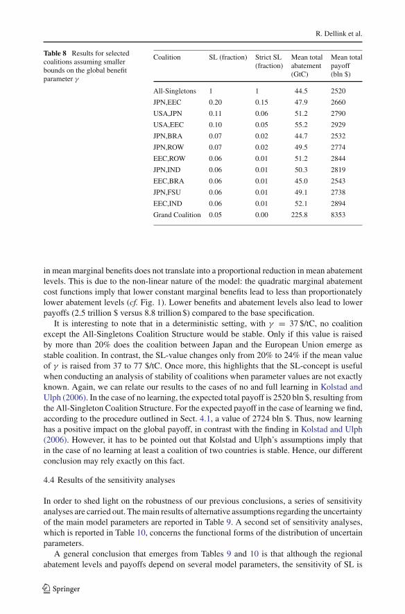
We expect that the probability density function of the global benefit parameter γ is crucialfor the analysis. Moreover, estimates of future benefits from abatement are widely acknowl-edged to be highly uncertain. Therefore, we carry out an alternative simulation with a differentassumption on the global benefit parameter γ . Table 8 shows results assuming that the 5 per-centile point is set to 0 $/tC and the 95 percentile point is set to 110 $/tC. This implies thatextreme values are rare and that the mean value of the global benefit parameter γ is reducedfrom 77 to 37 $/tC. Note that in the STACO model, a lower mean value of γ has a similarimpact as raising the discount rate as explained in Weikard et al. (2006) : as benefits fromabatement will occur later than the associated costs, a higher discount rate implies a smallerweight of (future) benefits and vice versa; see also the discussion of equation [4a]. Thus,the discount rate is not explicitly subjected to a sensitivity analysis, but only implicitly. Thespecific values considered here correspond to raising the discount rate from 2 to 7 percent.10

For all coalitions, the SL is lower than in the base specification. This is partly due to thelower probability of negative marginal benefits (this probability is reduced to 5%) and partlydue to the fact that mostly positive outliers of marginal benefits are removed from the model.The ranking (in terms of SL) of different coalitions is largely unchanged, implying that onlythe quantitative but not the qualitative conclusions are affected.

The lower mean value of γ reduces equilibrium abatement. In the All-Singletons CoalitionStructure, global abatement drops from around 70 GtC per century to 45 GtC. The reduction

10 Analogous to the procedure explained in note 5, we can also mimic these results using the Ramsey rule;the associated pure rate of time preference equals 5.2%.

123

R. Dellink et al.

Table 8 Results for selectedcoalitions assuming smallerbounds on the global benefitparameter γ

Coalition SL (fraction) Strict SL Mean total Mean total(fraction) abatement payoff

(GtC) (bln $)

All-Singletons 1 1 44.5 2520

JPN,EEC 0.20 0.15 47.9 2660

USA,JPN 0.11 0.06 51.2 2790

USA,EEC 0.10 0.05 55.2 2929

JPN,BRA 0.07 0.02 44.7 2532

JPN,ROW 0.07 0.02 49.5 2774

EEC,ROW 0.06 0.01 51.2 2844

JPN,IND 0.06 0.01 50.3 2819

EEC,BRA 0.06 0.01 45.0 2543

JPN,FSU 0.06 0.01 49.1 2738

EEC,IND 0.06 0.01 52.1 2894

Grand Coalition 0.05 0.00 225.8 8353

in mean marginal benefits does not translate into a proportional reduction in mean abatementlevels. This is due to the non-linear nature of the model: the quadratic marginal abatementcost functions imply that lower constant marginal benefits lead to less than proportionatelylower abatement levels (cf. Fig. 1). Lower benefits and abatement levels also lead to lowerpayoffs (2.5 trillion $ versus 8.8 trillion $) compared to the base specification.

It is interesting to note that in a deterministic setting, with γ = 37 $/tC, no coalitionexcept the All-Singletons Coalition Structure would be stable. Only if this value is raisedby more than 20% does the coalition between Japan and the European Union emerge asstable coalition. In contrast, the SL-value changes only from 20% to 24% if the mean valueof γ is raised from 37 to 77 $/tC. Once more, this highlights that the SL-concept is usefulwhen conducting an analysis of stability of coalitions when parameter values are not exactlyknown. Again, we can relate our results to the cases of no and full learning in Kolstad andUlph (2006). In the case of no learning, the expected total payoff is 2520 bln $, resulting fromthe All-Singleton Coalition Structure. For the expected payoff in the case of learning we find,according to the procedure outlined in Sect. 4.1, a value of 2724 bln $. Thus, now learninghas a positive impact on the global payoff, in contrast with the finding in Kolstad and Ulph(2006). However, it has to be pointed out that Kolstad and Ulph’s assumptions imply thatin the case of no learning at least a coalition of two countries is stable. Hence, our differentconclusion may rely exactly on this fact.

4.4 Results of the sensitivity analyses

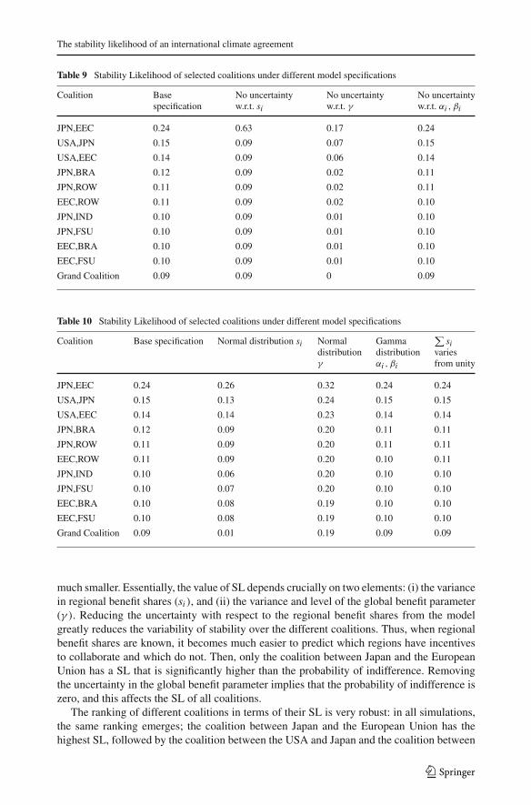
In order to shed light on the robustness of our previous conclusions, a series of sensitivityanalyses are carried out. The main results of alternative assumptions regarding the uncertaintyof the main model parameters are reported in Table 9. A second set of sensitivity analyses,which is reported in Table 10, concerns the functional forms of the distribution of uncertainparameters.

A general conclusion that emerges from Tables 9 and 10 is that although the regionalabatement levels and payoffs depend on several model parameters, the sensitivity of SL is

123


Table 9 Stability Likelihood of selected coalitions under different model specifications

Coalition Base No uncertainty No uncertainty No uncertaintyspecification w.r.t. si w.r.t. γ w.r.t. αi , βi

JPN,EEC 0.24 0.63 0.17 0.24

USA,JPN 0.15 0.09 0.07 0.15

USA,EEC 0.14 0.09 0.06 0.14

JPN,BRA 0.12 0.09 0.02 0.11

JPN,ROW 0.11 0.09 0.02 0.11

EEC,ROW 0.11 0.09 0.02 0.10

JPN,IND 0.10 0.09 0.01 0.10

JPN,FSU 0.10 0.09 0.01 0.10

EEC,BRA 0.10 0.09 0.01 0.10

EEC,FSU 0.10 0.09 0.01 0.10

Grand Coalition 0.09 0.09 0 0.09

Table 10 Stability Likelihood of selected coalitions under different model specifications

Coalition Base specification Normal distribution si Normal Gamma∑

sidistribution distribution variesγ αi , βi from unity

JPN,EEC 0.24 0.26 0.32 0.24 0.24

USA,JPN 0.15 0.13 0.24 0.15 0.15

USA,EEC 0.14 0.14 0.23 0.14 0.14

JPN,BRA 0.12 0.09 0.20 0.11 0.11

JPN,ROW 0.11 0.09 0.20 0.11 0.11

EEC,ROW 0.11 0.09 0.20 0.10 0.11

JPN,IND 0.10 0.06 0.20 0.10 0.10

JPN,FSU 0.10 0.07 0.20 0.10 0.10

EEC,BRA 0.10 0.08 0.19 0.10 0.10

EEC,FSU 0.10 0.08 0.19 0.10 0.10

Grand Coalition 0.09 0.01 0.19 0.09 0.09

much smaller. Essentially, the value of SL depends crucially on two elements: (i) the variancein regional benefit shares (si ), and (ii) the variance and level of the global benefit parameter(γ ). Reducing the uncertainty with respect to the regional benefit shares from the modelgreatly reduces the variability of stability over the different coalitions. Thus, when regionalbenefit shares are known, it becomes much easier to predict which regions have incentivesto collaborate and which do not. Then, only the coalition between Japan and the EuropeanUnion has a SL that is significantly higher than the probability of indifference. Removingthe uncertainty in the global benefit parameter implies that the probability of indifference iszero, and this affects the SL of all coalitions.

The ranking of different coalitions in terms of their SL is very robust: in all simulations,the same ranking emerges; the coalition between Japan and the European Union has thehighest SL, followed by the coalition between the USA and Japan and the coalition between

123

R. Dellink et al.

the USA and the European Union. Thus, we can conclude that SL provides a highly robustindicator of the stability of climate coalitions.

This is also confirmed in the last column in Table 10 where the assumption is given up thatthe sum of regional benefit shares is one. Thus, global benefit levels vary not only with thevariations in the global benefit parameter, but also with the sum of the regional shares. It turnsout that this assumption was not important: results are very similar to the base specification.

5 Discussion

This paper investigated the formation and stability of coalitions to reduce the negative impactsof climate change. We introduced a methodology to calculate the stability of all possible coa-lition structures in a stochastic, empirical setting. The concept of SL provided a notion ofstability that conveyed much more relevant information than the ordinary binary outcome:stable/unstable. The numerical application showed that the SL-concept contributes to a betterunderstanding of stability of coalitions when there is uncertainty about model parameters: itconstitutes a superior alternative to running numerous sensitivity analyses in a deterministicsetting.

The results suggested that for most possible climate coalition there is at least one regionthat is better off by changing its actions, thereby rendering coalitions unstable. This includedimportant coalitions such as the coalition of industrialised countries and the Grand Coalition.The lack of stability was very robust and held for a wide range of possible values for regionalabatement costs and benefits, as described by the respective probability distribution func-tions. There were only a small number of coalitions with a (strict) SL significantly differentfrom zero. Only when benefits from abatement are zero or negative (calibrated to be around9 percent in the base specification), i.e. when climate change does not pose a problem, willregions be indifferent between cooperation and no cooperation. However, in such cases, theoptimal abatement levels were zero, regardless of which coalitions formed.

The coalition with the highest SL was the coalition of Japan and the European Union, withan SL equal to 24% in our base case. This relatively low percentage stressed the difficulties instriking an international environmental agreement. This coalition but also the other coalitionswith a positive SL hardly improved over the All-Singletons Coalition Structure, correspond-ing to the case of no cooperation: global abatement and global welfare were only slightlyhigher than when there was no international collaboration at all, confirming a conclusion inthe literature derived with deterministic models.

The calculated SL of different coalitions was robust in terms of the considered distributionfunctions of parameter values, the variance in regional abatement costs and the global levelof benefits from global abatement, but was sensitive to the variance in the regional distri-bution of benefits. Unfortunately, regional benefits from abatement are very uncertain, andinternational research on adaptation and damage costs is still in its infancy. Therefore, it isof utmost importance to get better information on regional benefits.

We also related our results to those derived from stylized models with ex-ante symmet-ric players which conclude that learning has a negative impact on the outcome of coalitionformation. It became apparent that our approach corresponds to the case of full resolutionof uncorrelated uncertainty with perfect learning, according to the classification in Kols-tad and Ulph (2006). This case could be compared to the case of no resolution of uncer-tainty where decisions on coalition membership have to be taken on the basis of expectedvalues. We showed that learning may not always have a negative impact on global wel-fare. This suggested that the conclusions derived from stylized models as for instance in

123


Na and Shin (1998), Kolstad and Ulph (2006) and Kolstad (2007) are sensitive to the under-lying assumptions.

There are many ways in which the analysis above can be ameliorated. Firstly, better esti-mates of the variance on regional benefits may be obtained via a meta-analysis of the existingliterature, similar to what Tol (2005) did for global benefits. Secondly, the empirical modelused to calculate the regional payoffs can be extended to a fully-fledged computable generalequilibrium model. Together, we expect that these two extensions will improve the empiricalvalidity of the numerical example. Thirdly, it would be interesting to consider the case ofpartial learning as analysed in Kolstad and Ulph (2006) in order to better understand the roleof learning. Finally, the analysis could be extended to decision making under uncertainty byincluding risk-aversion of players as for instance considered in Endres and Ohl (2003).

Appendix 1. Histograms of the uncertain model parameters

Fig. A.1 Histogram of the global benefit parameter (γ )

Fig. A.2 Histogram of the regional benefit parameters (si ) for USA and China, respectively

123

R. Dellink et al.

Fig. A.3 Histogram of the regional abatement cost parameter (αi ) for USA and China, respectively

Acknowledgements Special thanks to Ivo Mulder and Kelly de Bruin for their research assistance and toEkko van Ierland, Eligius Hendrix, John Janmaat and two anonymous referees for their comments; the usualdisclaimer applies.

References

Babiker MH, Reilly JM, Mayer M, Eckaus RS, SueWing I, Hyman RC (2001) The MIT emissions predictionand policy analysis (EPPA) model: revisions, sensitivities and comparison of results. Joint program onthe science and policy of global change Report, 71. MIT, Cambridge

Barrett S (1994) Self-enforcing international environmental agreements. Oxford Economic Papers 46:878–894Bosello F, Buchner B, Carraro C (2003) Equity, development, and climate change control. J Euro Econ Assoc

1:601–611Botteon M, Carraro C (1997) Burden-sharing and coalition stability in environmental negotiations with asym-

metric countries. In: Carraro C (ed) International environmental negotiations: strategic policy issues.Edward Elgar, Cheltenham 26–55

Carraro C, Siniscalco D (1993) Strategies for the iternational potection of the environment. J Publ Econ 52:309–328

Dellink RB, Finus M, van Ierland EC, Altamirano J-C (2004) Empirical background paper of the STACOmodel, available on the STACO website http://www.enr.wur.nl/uk/staco, Wageningen University

Ellerman AD, Decaux A (1998) Analysis of post-Kyoto CO2 emissions trading using marginal abatementcurves. Joint program on the science and policy of global change Report, vol 40. MIT, Cambridge

Endres A, Ohl C (2003) International environmental cooperation with risk aversion. Int J Sustain Develop6:378–392

Eyckmans J, Finus M (2006) Coalition formation in a global warming game: how the design of protocolsaffects the success of environmental treaty-making. Nat Resour Model 19:323–358

Fankhauser S (1995) Valuing climate change. Earthscan, LondonFinus M, van Ierland EC, Dellink RB (2006) Stability of climate coalitions in a cartel formation game. Econ

Govern 7:271–291Hoel M (1992) International environment conventions: the case of uniform reductions of emissions. Environ

Resour Econ 2:141–159Kolstad CD (1996) Fundamental irreversibilities in stock externalities. J Publ Econ 60:221–233Kolstad CD (1996) Learning and stock effects in environmental regulation: the case of greenhouse gas emis-

sions. J Environ Econ Manage 31:1–18Kolstad CD (2007) Systematic uncertainty in self-enforcing international environmental agreements. J Environ

Econ Manage 53:68–79Kolstad CD, Ulph A (2006) International environmental agreements under uncertainty when learning reveals

differences between countries, paper presented at the conference “Learning and climate change”. IIASA,Laxenburg, Austria

123


Manne AS, Mendelsohn R, Richels RG (1995) Merge:a model for evaluating regional and global effects ofGHG reduction policies. Energy Policy 23:17–34

Metz B, Davidson O, Swart R, Pan J (eds) (2001) Climate change 2001: mitigation. Cambridge UniversityPress, Cambridge

Na S, Shin HS (1998) International environmental agreements under uncertainty. Oxford Economic Papers50:173–185

Nagashima M, Dellink RB, van Ierland EC (2006) Dynamic transfer schemes and stability of internationalclimate coalitions. Mansholt Discussion Paper 23, Wageningen

Nordhaus WD (1994) Managing the global commons. MIT Press, CambridgeNordhaus WD, Boyer J (2000) Warming the world: economic models of global warming. MIT Press, Cam-

bridgeOlieman NJ, Hendrix EMT (2006) Stability likelihood of coalitions in a two-stage cartelgame: an estimation

method. Euro J Oper Res 174:333–348Roughgarden T, Schneider SH (1999) Climate change policy: quantifying uncertainties for damages and opti-

mal carbon taxes. Energy Policy 27:415–429Tol RSJ (1997) A decision-analytic treatise of the enhanced greenhouse effect. PhD. Thesis. Vrije Universiteit,

AmsterdamTol RSJ (2001) Climate coalitions in an integrated assessment model. Computat Econ 18:159–172Tol RSJ (2002) Estimates of the damage costs of climate change: part 1: benchmark estimates. Environ Resour

Econ 21:47–73Tol RSJ (2005) The marginal damage costs of carbon dioxide emissions: an assessment of the uncertainties.

Energy Policy 33:2064–2074Ulph A (2004) Stable international environmental agreements with a stock pollutant, uncertainty and learning.

J Risk Uncertain 29:53–73Ulph A, Maddison D (1997) Uncertainty, learning and international environmental policy coordination. Envi-

ron Resour Econ 9:451–466Ulph A, Ulph D (1997) Global warming, irreversibility and learning. Econ J 107:636–650Weikard H-P, Finus M, Altamirano-Cabrera JC (2006) The impact of surplus sharing on the stability of inter-

national climate coalitions. Oxford Econ Papers 58:209–232Weitzman ML (1998) Why the far-distant future should be discounted at its lowest possible rate. J Environ

Econ Manage 36:201–208Weitzman ML (2001) Gamma discounting. Am Econ Rev 91:260–71

123

the stability likelihood of an international climate

Documents