the standard errors of various test statistics >-when the ... · the standard errors.of various...
TRANSCRIPT

THE STANDARD ERRORS OF VARIOUS
TEST STATISTICS
>-WHEN THE TEST ITEMS ARE SAMPLED
A Technical Report
prepared by
FREDERIC M. LORD
Office of Nay»! Research Contract Nonr-6g4(@o)
Project DesigsEfkö NR lf>413
EDUCATIONAL TESTING SERVICE
PRINCETON, NEW JERSEY
December, 1953
THE STANDARD ERRORS.OF VARIOUS TEST STATISTICS
WHEN THE TEST ITEMS ARE SAMPLED
A Technical Report
prepared by
FREDERIC M. LORD
Office of Naval Research Contract Nonr-694(00)
Project Designation NR 151-113
EDUCATIONAL TESTING SERVICE
Princeton, New Jersey
December, 1953
THE STANDARD ERRORS OF VARIOUS TEST STATISTICS
WHEN THE TEST ITEMS ARE SAMPLED
Frederic M. Lord
Abstract
Suppose that a large number of forms of the same test are administered to the same group of examinees, each form consisting of a random sample of Items drawn from a common pool of Items. If some test statistic is com- puted separately for each form of the test, the value obtained will (ig- noring practice effect, fatigue, etc.) differ from form to form because of sampling fluctuations. The standard deviation of the values obtained represents, approximately, the standard error of the test statistic when the test items are sampled.
Formulas for such standard errors are here derived for a) the test score of a single examinee, b) the mean test score of a group of exami- nees, c) the standard deviation of the scores of the group, d) the Kuder-Richardson reliability of the test, formula 20, e) the Kuder- Richardson reliability, formula 21, f) the test validity. In large samples, the foregoing statistics (with the possible exception of d) are approximately normally distributed, so that significance tests can be made by familiar procedures.
Consideration is given to the relation of certain of the foregoing standard errors to the conventional standard error of measurement, to the Kuder-Richardson reliability coefficients 20 and 21, and to the Wilks-. Votaw criterion for parallel tests. Practical applications of the results are briefly discussed. In particular, it is concluded that the Kuder- Richardson formula«21 reliability coefficient should properly be used in certain practical situations instead of the commonly preferred formula-20 coefficient.
THE STANDARD ERRORS OF VARIOUS TEST STATISTICS
WHEN THE TEST ITEMS "ARE SAMPLED*. 7'
Frederle Jl^ iord
._. ?_Suppose "thartr-She same tWt is adminle^ered to' a large number of
separate groups of examinees, the groups being random samples all drawn
from the same population; and suppose that some teat statistic is com-
puted separately for each sample of examinees, The value obtained for
this test statistic will, of course, differ from sample to sample be-
cause of sampling fluctuations. The standard deviation of these values
over a very large number of samples is the standard error of the test
statistic when examinees are sampled. For convenience, this type of
sampling will be referred to as type 1 sampling.
On the other hand, suppose that a large number of forms of the
same test are administered to the same group of examinees, each form
consisting of a random sample of items drawn from a common population
of items; and suppose that seme test statistic is computed separately
for each form of the test. Let us assume for theoretical purposes
that the examinees do not change in any way during the course of test-
ing;, i.e., that there is no practice effect, no fatigue, etc. The value
computed for the teBt statistic will still, of course, differ from form
to form because of sampling fluctuations. The standard deviation of
these values u<rer a very large number of samples is the standard error
of the test statistic when the test items are sampled. This type of
sampling will be referred to as a type S sampling. Test forms con-
structed by type 2 sampling will be called randomly parallel forms or
randomly parallel tests.
The writer is indebted to Professor S.S. Wilks who has checked over certain critical portions of a draft of this paper.

Type. 1 standard error f oxisulas have long been av&il«ä)l8 and, ar«*
sometimes incorrectly used in situations where sampling of test items
is of crucial, issporiaace. The present paper is concerned with deriv-
ing formulas for the type 2 steMärd 'etfQTBTot766Xi^M\^m%:ß^&§i^lQB.*
Formulas for the two kinds of standard errors may usually he readily
distinguished on a superficial level hy the following characteristics»
which underscore the essential difference "between thea: type 1 stand«
sard errors are usually obviously proportional to some power (positive
or negative) of the number of examinees in the sample — most commonly
inversely proportional^ to the square root of this number — and are
usually much less obviously and simply related, if at all, to the
number of items in the test; type 2 standard errors have the corre-
sponding characteristic with respect to n , the number of item« in
the sample.
Notation and Summary of Formulas
The test statistics with which the present study is concerned
are^prlmarily the following t
t — the observed test score of examinee a , obtained by a ,
counting the number of items answered correctly on &
single test. __*
£ — the mean of the scores obtained by the N examinees on
a single test. t = St /N . a a
s, — the standard deviation of the scores obtained by the S
2 2 / F2 examinees on a single test. s, •» £t /N - t
t a a

r21 "" *ne Kuder-Hlchs-xdson reliability coefficient* formula 231«
21 n-1 Lx ^n '/ua
r or r^j — the Kuder-Richardson reliability coefficient,
formula 20. r - -~=j» (l - £s "/s.) (symbols explained
in the succeeding list).
r . — the correlation of the test score with any external ex
variable, c . rct - sct/scst •
Considerable care in defining notation must he taken here in order
to avoid serious confusion. Additional symbols that will be used are
listed below for easy reference.
x. — the "score" of examinee a on item i . x. — 1 if ia la
the item is answered correctly. x. m 0 otherwise.
n — the number of Items in a single form of a test, i.e., in
a single sample. The subscript i runs from 1 to n .
H — the number of examinees in a single group of examinees.
The subscript a runs from 1 to N .
m — the number of items in a finite population of items.
p. — the observed "difficulty" of item i for the H exami-
nees tested. p. « ^loA •
%-1-P-i •
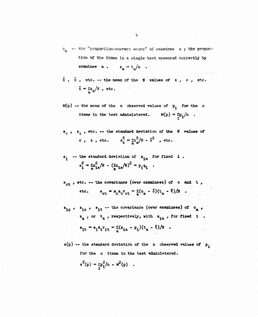
i — the "proportion-correct score" of examinee a j the propor-
tion of the Items in a single test answered correctly by
examinee a » z «• t /n . a a
E , c , etc« — the mean of the N values of % P c t etc.
z •• Ez /N , etc. a a
M(p) — the mean of the n observed values of p. for the n
items in the test administered. M(p) • £p, /n . i x
s.s, etc. — the standard deviation of the N values of c ' z
c , z , etc. s„ = EZ^/N - i , etc. * z a a
s. — the standard deviation of x. for fixed i i la
e . , etc. — the covariance (over examinees) of c and t ,
etc. sct - scstrct - S(ca - c)(ta - t)^ .
s. , s. , s.. — the covariance (over examinees) of c ,
z , or t , respectively, with x. f for fixed 1 . a a xa
ait- wit - 5(xia - >i>c*. - *)A ;
s(p) — the standard deviation of the n observed values of p.
for the n items in the test administered.
2/ !(p) - Zp^/n - ^(p) .

(slz) * 8(8it^ * e-fcc* •"" the standard deviation of the a
observed values of e. , s.. , etc» for the n items in Is * it *
the test administered. s (s±t) * Esft/a - (Es^/a)
s(s.c,s.,) -- the covariance (over items) of s. and s..
8(sic>8it) * ficsit/n - ^fic/n)(fit/n> •
**.,_ , *.<+ > r.i — the correlation of c , t t or z„ , •i.e. XX x.£ Et 6, 'el
respectively with x , for fixed i . r,. «• •Vt'*l8t
It should be noted that all the statistics in the foregoing list
are observed sample statistics relating to a given sample. There are
two kinds of statistics listed, typified, in the simplest case, by
I • Zz /N and M(p) ** £p./n . Population parameters have not been a a i 1
listed but -will be designated, vhen needed, by the use of Greek letters,
The following additional symbols, relating to the totality of all pos-
sible samples of test items (type 2 sampling), vill be used.
E(x) — the expected value of x j the arithmetic mean of the
statistic x over all possible samples.
S.E.(x) — the standard error of the statistic x j the standard
deviation of the statistic x
S.E.2(x) =E(x2) -CE(x)32 .
deviation of the statistic x over all possible samples. 2r~\ « w„2\ _ rw„\~!2
2/ v Var x — the sampling variance. Var x ~ S.E. (x) .
Cov(x,y) — the sampling covariance of the statistics x and y
ever all possible samples. Cov(x,y) = E(xy) - E(x)E(y) •
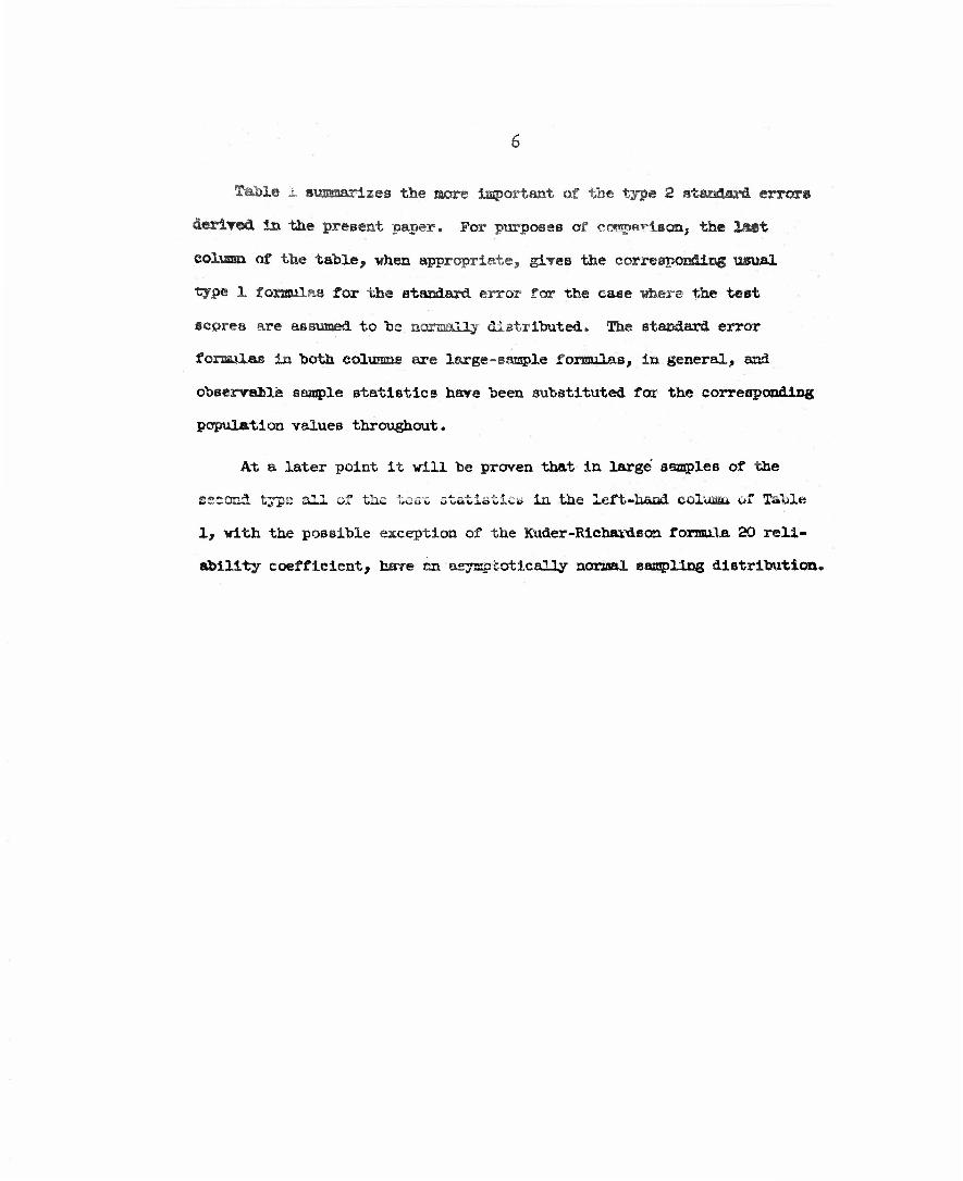
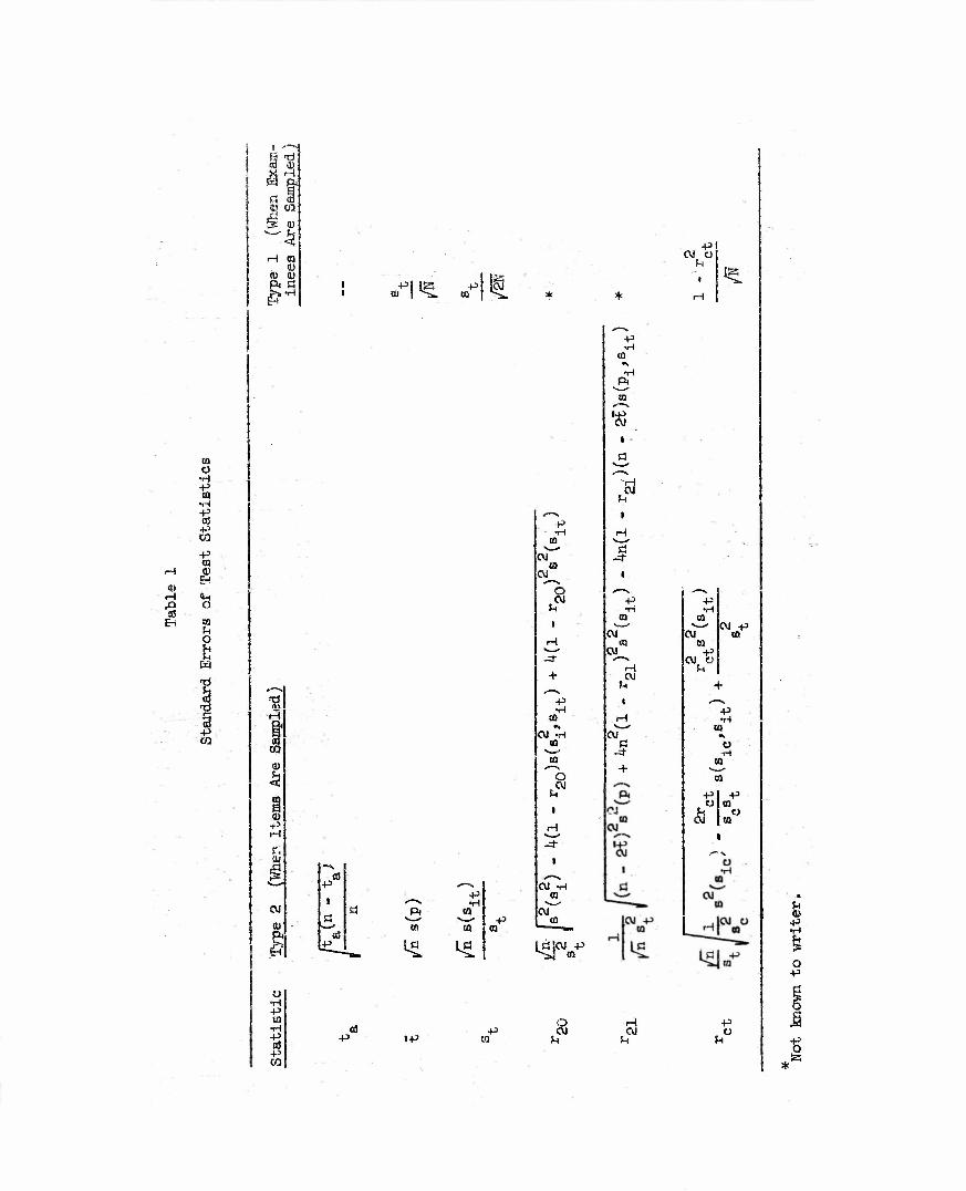
Table I maaaarlzes the more important of toe type 2 standard errors
derived la the present paper. For purposes of comparison, the last
column of the table, when appropriate^ gives the corresponding usual
type 1 formulas for the standard error for the case -where the test
scores are assumed to he normally distributed. The standard error
forasulas in both columns are large-sample formulas, in general, and
observable sample statistics have been substituted far the corresponding
population values throughout.
At a later point it will be proven that in large samples of the
second type all of the tea* statistics in the left-hand column of Table
1, with the possible exception of the Kuder-Richardson formula 20 reli-
ability coefficient, hare an aeysg? cot leal 1y normal sampling distribution.
OJ H •8 EH
CQ
O •H -P
CO •H
ti •p 00
+5 CO (1)
o CO u o
m
ä
1 CO
i •d ca 4)
tf H ft
fl § a.) CQ
s 0)
3 H (Q
V <t> 0) 1 Ö
•H
i CO
4 «a
r.
OJ
ft
•3 p •H
t£ L*
CVJ (a cw o CVJ u
i
H -sir
+
CVJ -H (0
HI
O OJ
u %
H ^?
l
CVJ -H CO
OJ
i£fV
p •H
•H
I
-H
J
CM Ft
CVJ a
-4"
P CVJ CJ
ft
n CVJ
CQ
-P CVJ O
CVJ p <0
p
M
o -rl
P Ü
CM t)
p
o p
CJ •H P CO •H •s p CQ
IP P
CQ
o CVJ CVJ
p o
u I
.la

7
Illustrative Examples and Discussion of the Standard Errors
Suppose that Form A of a certain 135-item test has.been administered.
Several parallel forms of this same teat are to be administered in the
future. Each form ia administered to a different group of examinees.
The groups of examinees may be considered as random samples drawn from
the Bame population. Each group ie so large that differences between
groups due to sampling of examinees may be ignored.* It is found that
th«? mean, standard deviation, and Kuder*Richardson formula 20 reliability
of the scores on Form A are 65.5, 21.5, and O.95, respectively. How much
may we -expect "Ehe mean» to vary from form to form?
The'required.-.value of s(p) can be determined directly from item
analysis dataj or it can be calculated from the three numerical values
given by solving for s (p) Tucker's modification (8) of the equation
for the Kuder^Rienardson formula 20 reliability, the result being:
', '.-•='". n
We find that s2(p) = .0538 .
The large-sample estimate of the type 2 standard error of the mean
is. found to be S.E.2(t) = 2.7 . (The subscript "2" is used here, and
the subscript "l" is used below, to indicate type 2 and type 1 standard
errors, respectively. Hereafter, type 2 sampling will be understood,
unless otherwise specifically indicated.) If the same test were admin-
•* Useful formulas for dealing simultaneously with sampling of items
and sampling of examinees have been developed by the writer for certain of the statistics studied here. Some such formulas are recently inde- pendently reported in Hooke, R., "Sampling from a matrix, with applica- tions to the theory of testing." Princeton University Statistical Re- search Group, Memorandum Report 53, 1953* (Dittoed.)

9
istered to random groups of 135 examinees, the type 1 standard error
would 'be B.E,.,(€) « 1,8 .
On the hasis of the foregoing, we may expect that parallel forms of
the test would not differ from each other in mean score by as much aB
2/äS„E.2{t) =7-6 points more than one time in twenty. If the parallel
forms are carefully constructed by matching items from form to form on
difficulty and item-test correlation rather than by random sampling of
items, it may well be that the forms will not differ from each other
as much as the foregoing formulas would indicate. On the other hand,
it is not unlikely that supposedly parallel forms of a test may, because
of the unconscious bias of the test constructor, often be found in fact
to be less parallel than would he expected if each form were a random
Sample of test"items.
In many kinds of statistical experiments it is commonly not merely
desirable hut actually necessary to select cases by randcsn sampling
rather than by stratified sampling, even though randan sampling gives
rise to larger sampling fluctuations. The reason is, first, that random
sampling tends to avoid unintentional hiasj and, second, that the stand-
ard errors arising from random sampling are known and easily used,
whereas those arising from stratified sampling are often either unknown
or excessively cumbersome to use. Similarly, and for the same reasons,
it will he desirable in certain kinds of experimental work, to use par-
allel forms composed of items selected at random rather than in any
other way.

Suppose, for example, it is desired to ir.vestigate the relation of
length of reading passage to validity in a reading comprehension test.
The experimenter might well select at random from a pool of all avail-
able reading items of some specified difficulty level (a) a sample of
all items based on passages containing more than 200 words and (b) a
sample based on passages containing less than 100 vords (it is assumed
here that there 1B only one item per reading passage). He then places
these items in random order and administers them to a group of examinees,
obtaining separate scores for the long and for the short items. He com-
putes the validity of each score, using some anefllable criterion. If
the two validity coefficients differ by little more than the type 2
Btandard error of their difference, it seems likely that the difference
is attributable to chance fluctuations due to the sampling of items.
If they differ by several times this standard error, the opposite con-
clusion may be reachedj Insofar as other uncontrolled experimental var-
iables are ruled out, the difference may plausibly be attributed to length
of reading passage.
A note of cautior. is necessary in using the type 2 standard error
formulas. These formulas involve no assumptions "beyond random sampling
and large n ; however, it is not at present known just how large an n
is needed in any given case. The formulas in Table 1, therefore, should
be used with some caution. Thiö Is particularly true of the last three
rows of the table, since the correlation coefficients given in the first
column UEadoubtedly have sharply skewed distributions when n is small.
It Bhould, finally, be noted that the assumption of random sampling
of items cannot be expected to hold for speeded tests, and the formulas
given in the present paper must be considered inapplicable.

10
Standard Errors of Measurement and TeBt Reliability
Table 1 gives a practical approximation to S.E»(t ) in terms of s,
observed sample statisticsj the rigorously accurate value, as Bhown in
a later section is
sjs.a(ta):-ira(n-ra)-. (2)
Here T "• E(t„) iö the true score of examinee a , i.e., the expected
value* of t over all randomly parallel forms of the test. The stand-
ard error of the score of an examinee is the standard deviation of the
errors of measurement of his score (error of measurement = t - T ). a a
The average of such standard deviations of errors of measurement over
all examinees,
r-*-X>-jg«v-*/ • ««
*The expectation symbol, E , denotes the average {afctMan&tic mean)
value over all type 2 samples. Thus the operator E can be treated by
the same rules as a summation sign, so that E(x + y) = E(x) + E(y) ,
EZ(t ) = ZE(t ) , E(nt) = nE(t) , E(T ) - T , etc. By def lition a Q, Q Et 8* EL
ra - E<ta) , s.E.2[f(tO - CfCt) - *{m)}f = E{f(t)}2 - &{t{t)}-f ,
and COT f1(t),f2(t)1 - EJf1(t)f2(t)"l - EIf^tjjUg(t)1 , where f (£)
is any function of t .
11
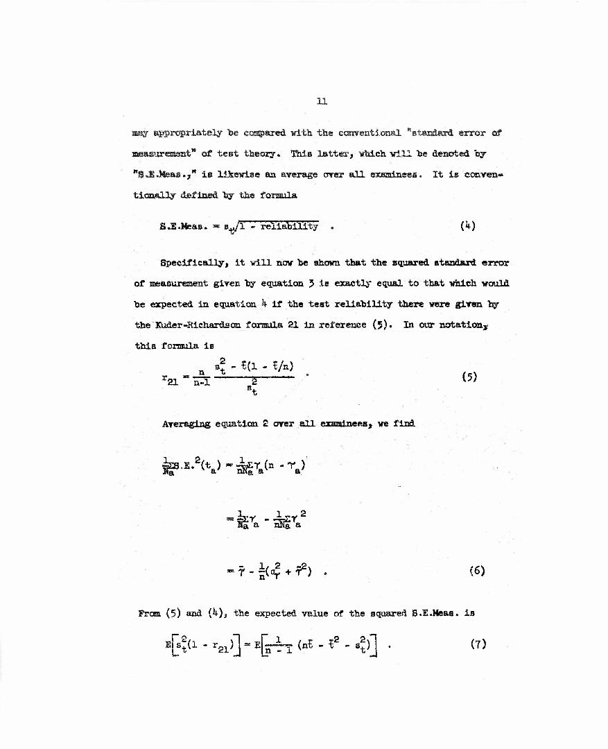
may appropriately fee compared with the conventional ^standard error of
measureaaant* of test theory» This latter, which will fee denoted ay
"8*I!.>§eaa.j" is likewise an average over all examinees. It is conven«
tionally defined fey the formula
S.E.Meas. m s^/l - reliability . {k)
Specifically, it will now he shown that the squared standard error
of measurement given hy equation 5 is exactly equal to that which would
he expected in equation k if the test reliability there were given fey
the Kuder-Richardson formula 21 In reference (5). In our notatioay
this formula is
sf - £(1 - I/o.) r21 n-1 2 W
8t
Averaging equation 2 over all examinees, we find
s 2(ta) * nla &<*-^)-äET«(n-ra)
l§ a nKa a
From (5) and {k)f the expected value of the squared S.E.Meas» is

la
In order to deal with (7) we first need, expressions far l(a. )
mtä. S(€)'
:«?>-• 1?*. " l>2] " #{(*« • V • (\ " « - « * «ft • <8>
After squaring ami rearranging I and £ signs,
2E(Ta - T)s{(ta - Ta)} - 2E{(1 - T)|(ta - Ya)} - 2E{(? - f)f(Ta - f)}]
(9)
How the fourth and the last terns on the right Yanish since E(t » f )
and 2(f » r) soth-equal sero. It is seen that we nave* terra, fox term» a a
E(s^) * jjp Var ta + o* + Var £ + 0 - 2 Var I - 0 (10)
Row Var t is given liy (2), so that EL
E<8t> ~ nlgra(n " ra) + 4 . Var £ (11)
Finally* proceeding as in (6), we hare
»(•*) = r . | ? + £~^ 4 . Var € (12)

Hext*
EC^2) - EßS - *r) + ff
«i(€ ~ r)2 + 2?E(£ » r) + E02)
Var £ •*• T2 . (13)
From (T), (12), and (13),
Thus result Is the sarae as that In (6). We hate shown that the arerage
squared standard error of igeasurement found. In type 2 sampling is exactly
equal to the expected rslue of the squared S.E.Weas. derived frcsa the
formi.Ta 21 Kuder-^Richardson reliability coefficient.
The logical relation between Kuder-Richardson fonnulas SO and 21
can be derived from equations 1 and 5, frcsa which it is readily found
that
»& ' r2Q> ~ Af± * r21> - Ä1! " (15)
How the term on the left and the first term on. the right of (15) are
the squared standard errors of measurement computed frcsa x^ and
from rp, , respectively* Furthermore, since ns /(n - l) is the
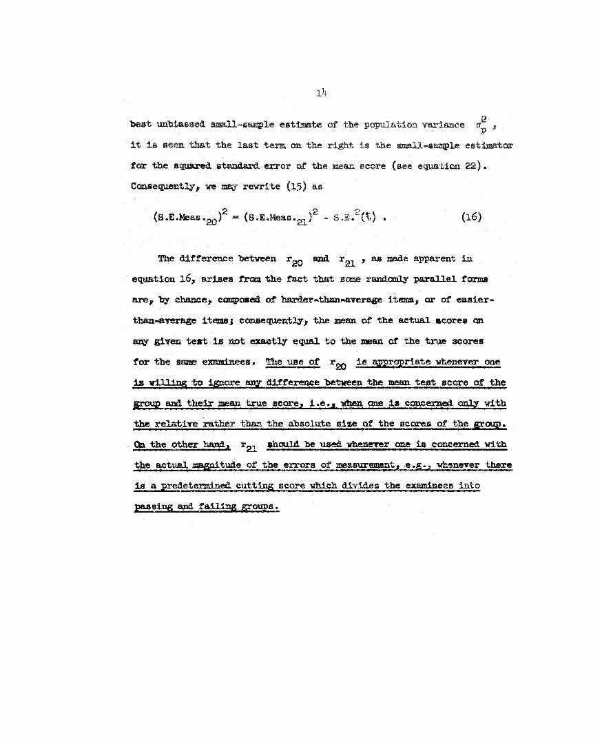
Ill-
•beat unbiassed sm&ll«gsaaple estimte of the population variance a t
it is seen that the last term on the right is the ssjalX-aiassple estimator
for the squared standard error of the mean score (see equation 22).
Consequently, we may rewrite (15) as
(S.I.Meas.20)2 * (S-E-Meas.^)2 - S.E.2(T,) . (i6)
The difference between r^ and r^ , as made apparent in
equation l6, arises from the fact that some randomly parallel forms
are, by chance, composed of harder-than-ÄTerage items, or of easier»
than-»average itemsj consequently, the mean of the actual scores on
any given test is not exactly equal to the mean of the true scores
for the same examinees» The use of r^ is appropriate whenever one
is willing to ignore any difference between the mean test score of the
group and "^eir ff68?* "*?"*? scop"5» i«8»,» ggggi v^ jg concerned only yltft
the relative rather than the absolute size of the scores of the group«
Oa the other hand, r^, should be used -whenever one is concerned -with
the actual magnitude of the errors of msaBurement, -e»g., whenever there
is a predetermined cutting score which divides the examinees into
passing and failing groups«
15
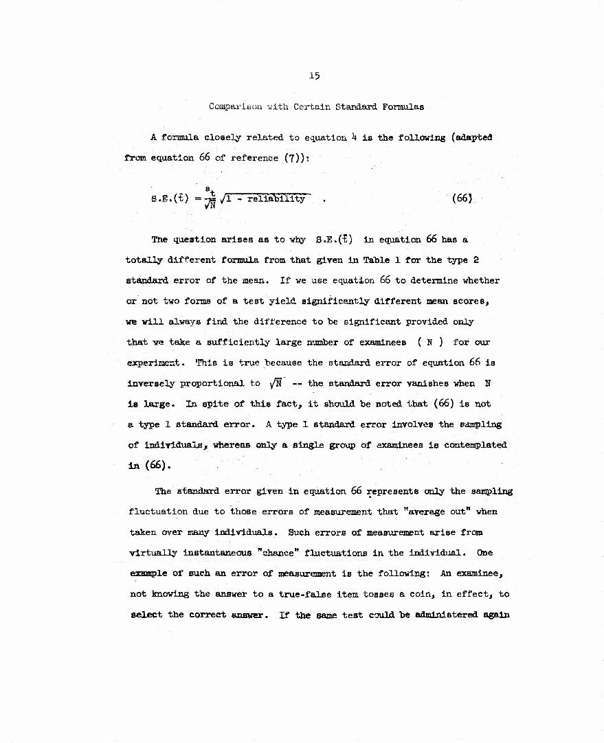
Comparison with Certain Standard Formulas
A formula closely related to equation k is the following (adapted
from equation 66 of reference (7)):
st , S=E.(t) ."»-TH/1 •- reliability . (66) vl
The question ariBea as to why S.E.(^) In equation 66 has a
totally different formula from that giren in Table 1 for the type 2
standard error of the mean. If we use equation 66 to determine whether
or not two forms of a test yield significantly different mean scores,
we will always find the difference to be significant provided only
that va take a sufficiently large number of examinees ( N ) for our
experiment. This is true because the standard error of equation 66 is
Inversely proportional to y^N — the standard error vanishes when N
1B large. In spite of this fact, it should be noted that (66) 1B not
a type 1 standard error. A type 1 standard error involves the sampling
of Individuals, whereas only a single group of examinees is contemplated
in (66).
The standard error given in equation 66 represents only the sampling
fluctuation due to those errors of measurement that "average out" when
taken over many individuals. Such errors of measurement arise from
virtually instantaneous "chanee" fluctuations in the individual. One
example of such an error of measurement is the following: An examinee,
not knowing the answer to a true-false item tosses a coin, in effect, to
select the correct answer. If the same test could be administered again
16
without practice effect, the same eytanlrVBCc.voiüA h&m a .fifty-fifty
chance of giving & different answer. This differeile gives rise to an
error of measurement of the type under discussion.
The standard error of the mean giv«a in Table 1 includes not osüy
sampling errors of the sort Just mentioned, hut also ssaiipling errors
arising from the sampling of the test items.
The line of reasoning applied to equation 66 is equally applicahle
to WlUcs' (10) and to Voters (9) significance tests when either of
these is used as a criterion of "parallelism" in tests, as suggested
hy Gulliksen (5> Ch. Ik), Gulliksen defines "parallel1' tests as having
equal means, equal -variances, and equal intercorrelations with each
other sad vith all external criteria (as well as satisfying appropriate
aon-statietical criteria of parallelism). Wilks1 and Votaw'a signifi-
cance tests provide rigorous statistical criteria for "parallelism"
under this definition. It would not he very desirable, however, to
apply Willa^, or Votaw,s procedures to data such as were obtained in the
second illustrative example given in a preceding section. If a test
composed of items having a certain characteristic is to he compared with
a test composed of different items having a second characteristic, it
may not he very useful to set up the null hypothesis that the two tests
are strictly interchangeable in every vay. Such a null hypothesis will
always be rejected if I is sufficiently large, but the rejection of
this hypothesis does not necessarily imply tnat the first and second
characteristics have different effect, since the observed discrepancy
might be readily accounted for as no greater than -would he expected to
be found in comparing two randomly parallel tests composed of the same
kind of items.
17
Sampling Distributions of Test Statiebics
It remains only to present the derivations of the results that have
up .;o now teen quoted without proof. The derivations are bbsedcTon the
assertion that there is a definite response ( x. } that a given examinee la
will make to a given item. The nature of this response may or may not be
known in advance. The group of N examinees to whom the items or tests
are administered is a fixed group not Bubject to sampling fluctuation or
other- changes.
The responses of the N examinees to item i may be specified by
the column vector -[x, = x ,x _, .. .,x "j- . Since each item response
is assumed to be treated as either "right" or "wrong", x. =0 or 1 ,
N and there are exactly 2 possible different vectors, i.e., different
patternc of item response. If we let the subscript I — 1,2,3,. ..,s ,
N then these possible patterns are represented by the 2 vectors x_
If two items have exactly the same pattern of responses, i.e., if the
response of each examinee is the same on both items, then the two items
are wholly indistinguishable in the present bituation. It may therefore
be asserted without loss of generality that, for present purposes, any
infinite pool of items is composed of £T different kinds of items,
designated by the 2T vectors xT . The relative frequencies of X
occurrence" of the different klnde of items are therefore the only
parameters needed to describe completely any infinite poolj these
parameters will be denoted by T_ , the relative frequencies of occur-
rence of the patterns x .
18
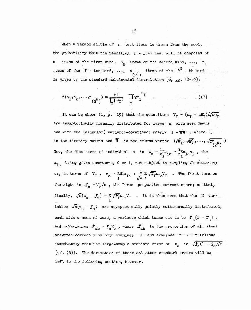
When a random sample of n test it eins is drawn from the pool,
the probability that the resulting n - item test will be composed of
n items of the first kind, np items of the second kind, ..., nT
items'" of the I - the kind, ,tli n J items of._the '..$ _.-__th kind: (2N)
is given by the standard multinomial distribution (6, p_£. 58-59):
•f(^"-^)) ~^f~T'1Tlr^1 ' (1T)
It can be shown (l, p. 419) that the quantities V_ = (n_ - nW-)/JnrL
are asymptotically normally distributed for large n with zero means
and with the (singular) variance-coyariance matrix I - TJ1T , where I
is the identity matrix and « iB the column vector {fä\> •JW^»'*<$ \JTF M ) 1 . (2W)
Now, the test score of individual a is z = —Ex. = —SxT n^. , the a n, X a n— xa x
xT being given constants, 0 or 1, not subject to sampling fluctuation;
or, in terms of VT , z = Etx. + — Z JlfLX-r VT . The first term on Ia_IIa/-TTIIaI I 4/n I
the right is S ^T /n , the "true" proportion-correct scorej so that, 3. EL
finally, \/ri(z - J' ) = T, v^xx VT • It is thus seen that the N var- a a _ X la j.
iables >/n(z - $ ) are asymptotically jointly multinormally distributed,
each with a mean of zero, a variance which turns out to be «T (l - $ } , cL £L
and covariances S . - t %, , where _f , is the proportion of all items ah a D ab
; answered correctly by both examinee a and examinee b . It follows
immediately that the large-sample standard error of z is ,/J" (1 - S )/n
(cf. (2)). The derivation of these and other standard errors will be
left to the following section, however.

19
$y a well-known theorem, If f(z.,z„?...,z ) is a function of the
z& having continuous first-order partial derivatives with respect to
each 2 at the point (j-^C,, »• •>lw) J aaä if a* least roe of these
derivatives is nonvanishing at this point, then the quantity ^ülfCs-,
zg>...,z„) - f(£i,»$2>. ••»§«) I is asymptotically normally distributed
with zero mean when n is sufficiently large. This theorem assures ua
that the mean score ( £ or t ), the standard deviation of the scores wmmmtmm —W—I M U • fww—M• nun ' •* ••mi »n, .. i. .- i • i n mi i i i i i ii MJ | HI r ii- ii mi mm r •.; n I mm '
( 8 or 8. ), the Kuder-Richardson formula 21 reliability ( r«,.) ,
and the test validity { r or r . ), are approximately normally
distributed in type 2 teampllag with large n j and in addition gives us
the large-sample expected value of each statistic. It seems highly
likely that the Kuder-Richardson reliability, formula 20, likewise is
asymptotically normally distributed, but no proof of this conclusion
is available at present, in view of the fact that the formula for this
2 statistic involves a (p) , which is not a function of the z .

20
Derivations of Expected Values and Standard Errors
The Individual 8eore
The proportion of the items in the entire pool to which examinee
a will give the correct answer is, by definition, 5 «• T /a . If Si &
n items are drawn at random frcm the pool, t , the score of examinee
a on the resulting test, i.e., the number of items that he will answer
successfully, will of necessity have the usual binomial distribution*
with mean and variance
E(ta) - ra , (18)
S.E.2(t ) -i Y (n - r ) = n? (1 - 9 ) . (19)
This conclusion (and also those that follow, except as large n may be
assumed) depends on no assumptions whatever except that of random sampling.
Equation 19 is identical with equation 2, which was discussed in a pre-
vious section. If the observed value t is substituted for the unknown a
T in (19 )t we obtain the square of the first formula of "able 1. El
For finite sampling, when n iteas are drawn without replacement
from a finite pool of m items, the corresponding formulas, stated with-
out proof, are
E(ta) - Tfi , (18*)
• I II L ' »•••••—• HP U III I I I > | I • I II • I I
If we concern ourselves with only a single examinee,* the number of
correct responses that he gives on one sessple of items is not correlated
with the number that he gives OH. other aamples.

21 *
S.E,2(t ) =5~T(ri -r ) . (19s) * a BSI a a V *
The Mean Score of. the Group Tested
It should he noted that the scores of examinees "a and b are
not independent over different parallel forms Of the test. If a
particular form happens to he composed of rather difficult items, hoth
examinees will tend to get low scores j if a particular form happens to
be easy, hoth will tend to score higher. Consequently, although the
expected value of the mean score in the group i s equal to the mean of
the expected values of the individual scores, i.e.,
E (^feTa = t > <20>
the standard error of the mean is not an average of the standard errors
of the individual scores.
It will he convenient from this point on to work with z ** t /n , EL EL
the proportion-correct score, rather than with t itself. The nature
of the desired standard error follows immediately from the fact that
the mean score ( z ) is identically equal to the average item difficulty
z = M(p) . (21)
The usual formulas for the standard error of a-mean apply to M(p) ,
so that
S.E.2(Z)=io2(p) (22)
where a(p) is the standard deviation of the item difficulties over
22
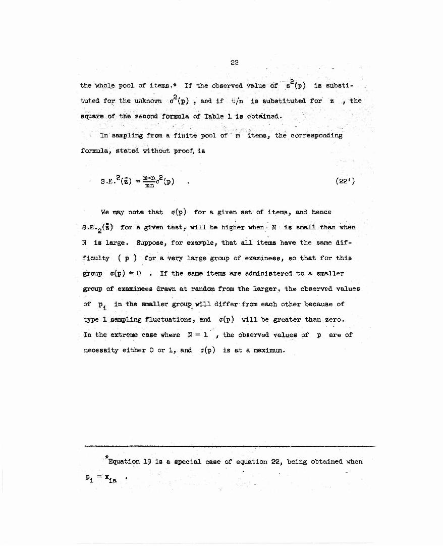
the whole pool of items.* If the observed value of s*(p) is substi-^
tuted for the unknown ff"(p) , and if t/n is substituted for z ,, the
square of the second formula of Table 1 is obtained.
In sampling from a finite pool of m items, the corresponding
formula, stated without proof, is
S.E.2(i) -2~£aS(p) . (22')
We may note that cr(p) for a given set of items, and hence
S.E.2(«) for a given test, will be higher when N is small than when
N is large. Suppose, for exaiyple, that all items have the same dif-
ficulty ( p ) for a very large group of examinees, so that for this
group a(p) * 0 . If the seme items are administered to a smaller
group of examinees drawn at random from the larger, the observed values
of p. in the smaller group will differ from each other because of
type 1 sampling fluctuations, and a(p) will be greater than zero.
In the extreme case where N = 1 , the observed values of p are of
necessity either 0 or 1, and a(p) is at a maximum.
* Equation 19 ia a special case of equation 22, being obtained when
Pi = Xia
23
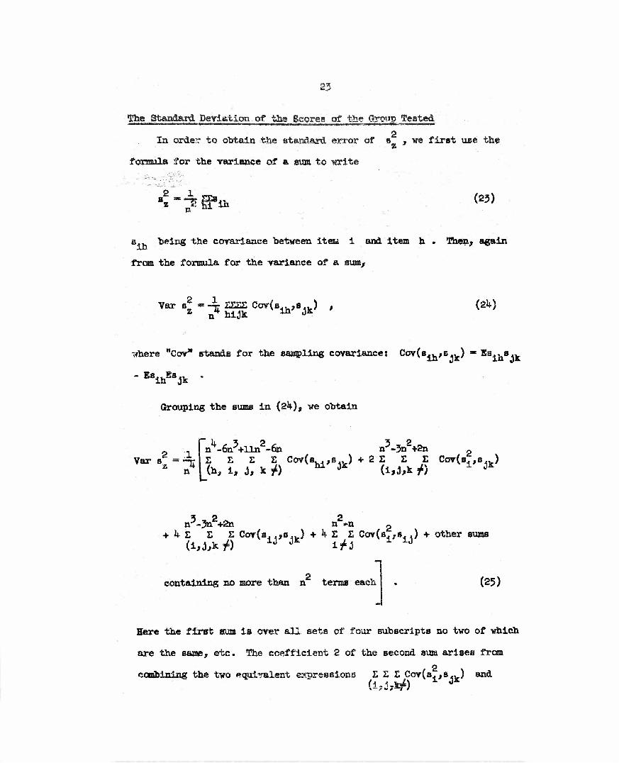
fite Standard Deviation of the Scores of tue Group Tested
2 la order to ohtain the standard error of t , we first use the
formula jfor the variance of a sum to write
•S-^fftt (23)
B.. "being the covarianee between item i and item h . Then, again
from the fornaila for the variance of a su%
Var s*~ 7 SS c^8ih^jk> ' n^ hijk (A)
where "Cov" stands for the Basiling covariancei Cov(8ii1'B4k^ * Esihs1k
" EßihEsjk *
Grouping the sums in (2k), we obtain
Var BZ - TJ n -6n +lln -6n n -5n +2n Z Z E E Cov(s. .,s,. ) + 2 E 2 E Cov(s,,s . ) (h, i, J, k )t) M J1C (i,J,k j*) Jt
n5-5nS+2n 2 n »n
+ 4 ZEE Cov(s. ,,s., ) + k E E Cov(s.,s. .) + other sums
containing no more than n terns each (25)
Here the firsrfc sum is over all sets of four subscripts no two of which
are the same, etc. The coefficient 2 of the second sum arises from
combining the two equivalent expressions E E E Cov(a,,s.v) and \ * 0 v if —"$ /

2k
Kg. fj8.)--••-, Hie other numerical coefficients arise similarly-
The polynomials in n «ritten abtw* the summation signs indicate the
number of terms liiYolTed in the BUBSsation»
Now, the terms '-nder each Buanaatl-an sign in (25) are all the same
no matter what the numerical values of the subscripts! consequently
z - Var s'_ =• -"* n
(n - 6rr -t lln - 6TJ,)COT(BL,,S.^) + 2(n - 3n • EnJCorCa^B.^)
+ Mn3 - 5n£ + 2n)Cov(a1J,sJk) + 0(n2) (26)
where 0(n ) stands for terms of order n . In (26) and in the follow-
ing paragraph it is understood that h,i,j,k^ .
Now, s. . uijd a., fluctuate independently over successive samples,
/ «. 2 so that CoT(sh.jS,. ) •» 0 . The same is true of a. and a,. . Con-
aequently,
Var s\ -4r ^ ' 5a2 • «a)Cor(«1J,«Jk) + PT^-^M«^«^) + cZ-U. (2?)
Equation 27 gives the desired result, but not in a very useful form,
since Cov(a..,s,. ) is a function of population parameters end is gener- ös
ally not known. As a final step, then, it will be shown that s (s. ) ,
the actual variance (over items 1 to n ) of the observed item-test
covariances, provides a "consistent" estimate of COV(B.,,B . ) , i.e.,
It will be proved that

25
.a <Bn> Cov-(Si^8jk) + o(|) . (88)
From the formula for the corarlanee of a earn»
*i*-|fij ' (29)
^"iz^^g^V8^ * (50)
the term under the summation sign, being the actual corarlanee (over
items 1 to n ) of the observed values of s. , and s^ t
B<«vV - Wik-?(?«)(?ik) (31)
Substituting from (31) into (30)/ and taking expected valuea, ve
find
"•^-^jyvn-^SS**''«* (»)
Grouping the sums on the right, we hare
rn(n-l)(n-2) 1 rn(n-l)(n-2)(n-3) E« (B..J "^ E E Z Es. ,B.. + 0(a*) - -4- LESE Is.,« ik
• 0(n5) (33)

Now, tbe tsnsw under each mmmtitm sign in (33) are the same re-
gardless of' the numerical value of the subscript. Furthermore > as already
pointed out in deriving (27). COV(B. .,8,.) = 0 when h^i^j,^ , or in
other worts, *B5t4*fv * EehjtEsik K° r <** £!shisiv ~ Es, J»»ik - Con-
sequently,
HB2(Bi2) - fc13.tt . ^ jEBik + 0 (i) • (54)
But this is the same as (28) * which was to he proved.
2 The large sandle standard error of 8^ may therefore be estimated
from the actual variance of the observed item-test covariancess
S.E.2(s^) «V(si2) . (35)
By meisns of the "delta" method (kf Vol. 1, gg, 208 ff.)? it is
readily shown from (35) that in large sampleB
S.E.2(s ) - J^.E.£(s2) - —|L . (36)
z z
If t/n is substituted for z in (3^)> the square of the third
equation of Table 1 ie obtained.
The corresponding squared standard error for sampling from finite
populations may be shown to he
"^•^\) ' <37)
27
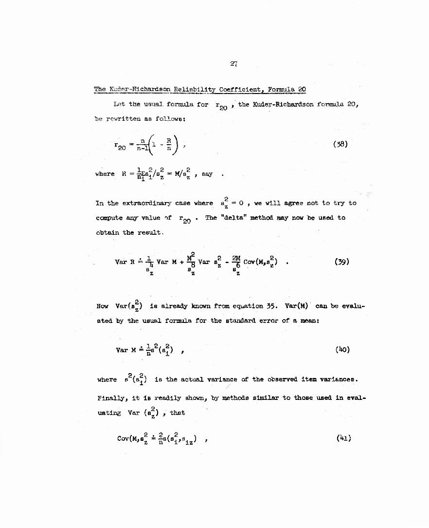
The Kader-Richardson Reliability Cqeffleientj Formula 20
Let the usual formula for V~Q t the Kuder-Richar&son formula 20i
be rewritten as fcHowsj
-ja/i-»^ n-ll n / r20 = "^ 1 * " ' ' Wl
1 ? / P P where R = ^Ja
z m M/8Z > say
2 la the extraordinary case where a ~ 0 , we will agree not to try to
2*
compute any value of r^ . The "delta" method may now he used to
obtain the result.
Var R A -L Var M + ^ Var s^ - ^ Cov(M,e^) , (39) s s s„ z z z
Now Var(s ) is already known from equation 55- Var(M) can be evalu- z
ated by the usual formula for the standard error of a mean:
VarM=is2(s2) , (1*0)
2 2 where s (s.} is the actual variance of the observed item vari&ncee.
Finally, it is readily shown, by methods similar to those used in eval- o.
uating Var (s"") , that z
Cov(M,s2 - |»("J»»U) , (*L)

28
'•Jhere s(s.,,s. ) is the actual oovarianee between the observed ite-n
variJya<s-#s and the observed item-test covariancesi
Consequently,'
Var K ns z
s2(s2) + ^R2s2(s. ) - 4RS(S
2,S. )~| . X IS 1 XZ I fl»)
Now Var(rpQ) = ~g Var(R) ; hence, to order l/n , n
•E.2(r2Q) '--^[".«(.J) + Un9(l - r20)
2s2{Blz) - «m(l - r^Ms2^)] . (43) n s <— —• '
It may be noted that the quantity (l - rp_) is of order l/n , because,
by the Spearman-Brown formula, lim n-(i~ - ron) - constant . It is then n=oo d°
see^from (^5) that S.E« (rori) is a auantity of order i/n . Equation
kj> leads directly to the fourth formula of Table 1.
It may be shown that the corresponding standard error when sampling
from a finite population is (m - n)/m times the value given in (^3).
The Kuder-Bichardson Reliability Coefficient, Formula 81
By a procedure wholly parallel to that used for the formula-20 relia-
bility coefficient, it is found that, approximately,
S.E.2(r21) - 1 f(i „ S5)2s2(p) + Un2(l - r21)2s2(3^
n s L,
- l+n(l - r21)(l - 2ä)s(pi,slz) w
where s(p ,s. ) 1B the actual covariance between the observed item X 12*
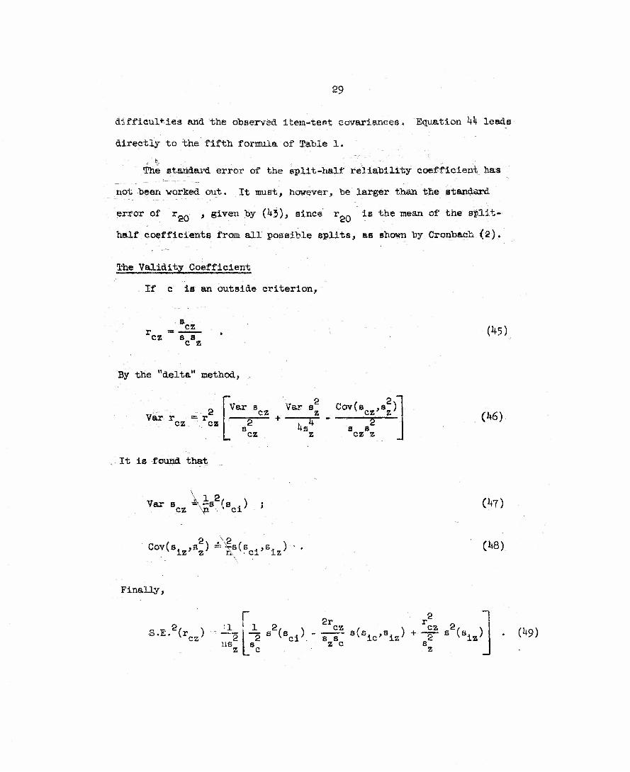
29
difficulties and the observed item-tent eovarlanees, 'Equation k\ leads
directly to the fifth formula of Table 1,
The standard error of the split-half reliability coefficient has
not been worked out. It must, however, be larger than the standard
error of r~Q , given by (h3)} since r^. ig the mean of the split*
half coefficients from all possible splits, as shown by Cronbach (2),
The Validity Coefficient
If c is an outside criterion,
r = cz cz s s
C 2
(V5)
By the "delta" method, ,
Var r —r cz cz
r„ „ 2 Var s var s cz z
s cz z
Cov(s ,s ) v cz' z —, r—
8 S CZ Z
<*6)
It is found that
Var Bcz ^s2(aci) '
Cov(s. ,a ) =;Vs(s 4,s, ) x iz7 z a • ci iz
(^7)
C*8).
FinaUy,
r S.E- (r ) cz us
1 2/ ,, "2 S <8ci>
2r r cz / \ cz 2, x. SIS, ,S. ) + —je- E (S. ) s s v ic' is' 2 v *-* z c s z
'iz' • (»*)
30
Equation h$ leads directly to the last formula of Table 1.
The corresponding standard error for sampling from a finite, p^ol
of items is presumably (m - n)/m times the foregoing quantity,
31
References
1. Cramer,, H. Mathematical methods of statistics. Princeton Univ.
Press, 1946.
2. Cronbach, L. J, Coefficient alpha and the internal structure of
tests, Fsychometrika, 1951, 1§* 897-3$** ..;
3. Gulliksen, H. Theory of mental tests, Nev Yorks Wiley, 1950.
k. Kendall, M. 0. The advanced theory of statistics. London;
Charles Griffin and Co., 19^8. 2 vols.
5. Kuder, G. F. and Richardson, M. W. The theory of the estimation
of test reliability. Psychometrika, 1937, 2, 15I-160.
6. Mood, A. M. Introduction to the theory of statistics. New York;
McGraw-Hill, 1950.
7. Peters, C. C and Van Voorhis, W. R. Statistical procedures and
their mathematical "bases. New York; McGraw-Hill, 19*0.
8. Tucker, L. R. A note on the estimation of test reliability by
the Kuder-Richardson formula (20). Psychometrika, 19^9»
ih, 117-119.
9. Vat'aw, D* F., Jr. Testing compound symmetry in a normal multi-
variate distribution. Ann, math. Statist., 19^, 19, M7-V73.
10. Wilks, S.S. Sample criteria for testing equality of means,
equality of variances, arid equality of covariances in a
normal multivariate distribution. Ann• math. Statist., 19^6»
17, 257-281.