The Stochastic Response Dynamic:

A New Approach to Learning and Computing

Equilibrium in Continuous Games

Amit GandhiUniversity of Chicago

Graduate School of Business

Abstract

This paper describes a novel approach to both learning and comput-ing Nash equilibrium in continuous games that is especially useful foranalyzing structural game theoretic models of imperfect competition andoligopoly. We depart from the methods and assumptions of the tradi-tional “Calculus” approach to computing equilibrium. Instead, we use anew and natural interpretation of games as conditionally specified proba-bility models to construct a simple stochastic learning process for findinga Nash equilibrium. We call this stochastic process the stochastic responsedynamic because of its resemblance to the classical Cournot best responsedynamic. The stochastic response dynamic has economic meaning as aformal learning model, and thus provides a rationale for equilibrium selec-tion, which is a major problem for the empirical application of structuralgame theoretic models. In addition, by way of its learning path, it providesan easy guide to check for the presence of multiple equilibria in a game.Finally, unlike the Calculus approach, the stochastic response dynamicdoes not depend upon the differentiability properties of the utility func-tions and makes no resort to the first order conditions of the underlyinggame.

1 Introduction

The traditional approach to computing a pure strategy Nash equilibrium incontinuous games 1 is to use certain standard tools from Calculus to set up andsolve a potentially nonlinear system of equations. More precisely, the “Calculusapproach” finds a Nash equilibrium by using a Newton-like method to search fora state of the game that simultaneously solves each player’s first order condition.

The Calculus approach suffers from some important shortcomings that hin-der its overall usefulness for economic analysis. First, numerical methods ofsolving systems of equations do not correspond to any kind of economicallymeaningful learning process, i.e., the underlying search for equilibrium is notdecentralized. At every step of the search, Newton’s method updates eachplayer’s action in a way that depends on the utilities of all the players. Onthe other hand, a decentralized approach to finding equilibrium requires thateach player’s choice of action depend only upon his own utility function. De-centralizing the search for equilibrium is the key feature of a learning model inEconomics[12].

For normative applications of game theory to the design of multi-agent sys-tems [20], a decentralized approach finding Nash equilibrium is essential. Forpositive applications, where structural game theoretic models are estimatedagainst data, and then used to analyze counterfactual states of the world, suchas mergers or the introduction of new products, a learning model that effec-tively computes equilibrium offers a natural solution to the problem of multipleequilibria and equilibrium selection. A major motivation for developing modelsof learning in games is to offer a framework for saying whether some equilibriaare more likely than others, depending on whether they can be learned in somenatural way [8].

The usefuleness of the Calculus approach for applied work is also limited bythe differentiability assumptions it imposes on the game. If utility functions ofthe underlying game are not differentiable, and/or the first order conditions arenot well behaved, then the Calculus approach can readily fail to find a Nashequilibrium.

This paper describes a novel approach to learning and computing Nash equi-librium that abandons the methods and assumptions of the traditional Calculusapproach. Instead, we use a new and natural interpretation of games as con-ditionally specified probability models to construct a simple stochastic processfor finding a Nash equilibrium. We call this stochastic process the stochasticresponse dynamic. The stochastic response dynanamic, unlike the Calculus ap-proach, searches for Nash equilibrium in a decentralized way2. Furthermore, the

1The term continuous games shall mean games with continous action sets and continuousutility functions. Throughout the paper, all games are implicitly assumed to be continuousgames.

2The bulk of the literature on learning in games is focused on finite games and mixedstrategy equilibrium. Our focus on learning pure strategy equilibrium in continuous games,which is the primary game theoretic framework used in empirical work, is a unique feature ofthe present work.

2

stochastic response dynamic does not require the utility functions of the gameto be differentiable and makes no resort to the first order conditons whatsoever.

The stochastic response dynamic is reminiscent of the well known best re-sponse dynamic. The best response dynamic, which dates back to the inceptionof game theory [3], is a simple (perhaps the simplest) model of learning in con-tinuous games. Starting from any initial state of the game, it specifies that theplayers will take turns choosing their best response to the state of the game inthe previous period. Of course, a player’s best response to a state of the gamedepends only upon his own utility function, and hence the process is decentral-ized. Further, if this process of iterative best responses settles down to a singlestate, then we know it has settled down to a Nash equilibrium.

Unfortunately the best response dynamic does not suffice as a general toolfor finding equilibrium because there is little guarantee that the process willever converge. Only under very special monotinicity assumptions on the game,such as supermodularity, can such a guarantee be made3.

The stochastic response dynamic is essentially a stochastic version of thebest response dynamic. Instead of players taking turns exactly best respondingto the state of the game in the previous period, the stochastic response dy-namic specifies that players behave by using stochastic responses. A stochasticresponse consists of the following. A player first randomly samples a candidateresponse from his action set. With this candidate response in hand, our playercan either continue to use his action from the previous period (and thereby rejecthis candidate response), or he can switch his action to the candidate response(and thereby accept the candidate response). Rather than necessarily choosingthe option that yields higher utility, our player probabilistically chooses betweenhis two possible responses. This choice probability is governed by the classicalbinary logit model.

The variance parameter in the logit choice probability can be interpreted asthe amount of noise entering the stochastic response dynamic. If the level ofnoise is infinitely large, then our player flips a fair coin in order choose betweenresponding using his previous period action or responding using his candidateresponse. As the level of noise decreases, the choice probabilities increasinglyfavor the response that yields the higher utility. In the limit, as the level ofnoise approaches zero, our player necessarily chooses the response that yieldsthe higher utility.

Thus the stochastic response dynamic maintains the decentralized natureof the best response dynamic, but replaces best responses with our notion ofa stochastic response. The key benefit achieved by replacing best responseswith stochastic responses is that it overcomes the major shortcoming of thebest response dynamic, namely its lack of convergence. For a fixed noise level,the stochastic response dynamic transforms the previously deterministic bestresponse dynamic into a stochastic process. The form of the stochastic processis a Markov chain, which unlike the deterministic best response dynamic, can be

3This lack of convergence problem holds true for fictitious play more generally, the bestresponse dynamic being an extreme form of fictitious play.

3

assured to uniquely converge. The convergence however is no longer to a singlestate of the game, but rather to a probability distribution over the possiblestates of the game. In the language of Markov chains, the stochastic responsedynamic is uniquely ergodic and converges strongly (in total variation norm) toa unique equilibrium distribution.

Our main results concern the relationship between the equilibrium distribu-tion of the stochastic response dynamic, and the Nash equilibria of the underly-ing game. Essentially, we argue that for the class of games over which we wishto to compute, the Nash equilibria of the game are the modes, or “centers ofgravity” of the equilibrium distribution. Furthermore we argue that as we de-crease the variance parameter of the logit choice probability, i.e., as we decreasethe amount of noise entering the stochastic response dynamic, the equilibriumdistribution becomes increasingly concentrated over its modes, and thus in thelimit, converges (in law) to a degenerate distribution over the Nash equilibriastates of the game. In the case of a unique Nash equilibrium, this limitingdistribution is simply a point mass over the Nash equilibrium.

Thus simulating the stochastic response dynamic at a fixed noise level as-ymptotically produces a random draw from the corresponding equilibrium dis-tribution. As the noise gets smaller, the probability that this equilibrium drawis further than an epsilon away from a Nash equilibrium goes to zero. Comput-ing Nash equilibrium amounts to simulating the stochastic response dynamicfor a fixed number of iterations, then decreasing the amount of noise accordingto some rate, and repeating the simulation. Simulating the stochastic responsedynamic at a given noise level will result in a sample being drawn from its equi-librium distribution. As we reduce the noise, this sample will be increasinglyconcentrated over Nash equilbrium states of the game. Once the simulationproduces a sample draw near one of the equilibria at a sufficiently small noiselevel, the simulation becomes “stuck” near this equilibria (i.e. all the candi-date responses will be rejected), and thus we have approximately computed anequilibria.

This process of adding noise or “heat” to a system, and reducing this heatso as to bring the system to its equilibrium resting state, has a long establishedhistory in thermodynamics. More generally, simulating Markov chains so asto compute scientific quantities of interest has gained much momentum in theStatistics and Physics literature over the past 50 years [10]. Usually known as“Markov Chain Monte Carlo”, the approach has been used to solve computa-tional problems that cause difficulty for gradient based numerical methods (i.e.the Calculus based approaches). The stochastic response dynamic follows inthe spirit of the Markov Chain Monte Carlo literature. In fact, the stochasticresponse dynamic is nothing more than an adaptation of the classic Metropolisalgorithm taken from statistical physics literature, except modified so as to beapplicable to strategic games.

The connection to the MCMC literature provides insights for improving thecomputational performance of the stochastic response dynamic. Markov ChainMonte Carlo is generally quick (efficient) to provide an approximate solution,but can be slower at providing a highly accurate one. A common approach in

4

the literature to improve upon this is to take a hybrid approach, using MCMCto generate a “close” answer to a problem, and then letting a traditional Cal-culus driven approach hone the accuracy of this approximate answer [1]. ThusIn terms of computing Nash equilibrium, the stochastic response dynamic canquickly generate an approximate equilibrium, which can be input as the startingvalue for a nonlinear equations solver that computes the solution to the systemof first order equations.

The plan of the paper is as follows. In section 2 we review strategic gamesand Nash equilibrium, and define the class of games G over which we wish tocompute, namely continuous/quasiconcave games. Section 3 reviews the fairlysimple minded, but nevertheless decentralized approach to finding equilibrium,the best response dynamic. In section 4, we see how the Calculus approach solvesthe lack of convergence problem of the best response dynamic. However theCalculus approach comes at the cost of not being decentralized, and requiringthat the first order conditions both exist and are well behaved.

In section 5, we introduce the stochastic response dynamic, which replacesthe best responses from the best response dynamic with stochastic responses.In section 6 we provide an intuitive view as to why the stochastic response dy-namic converges to Nash equilibrium by introducing a restrictive assumptionon the game known as compatibility. In section 7, we drop the compatibilityassumption and replace it with the more natural Nash connectedness assump-tion, which we conjecture holds true generically for games in G (and can proveit holds true for 2 player games in the class). The convergence properties of thestochastic response dynamic are shown to hold equally under connectedness ascompatibility. In section 8 we begin to illustrate the computational behavior ofthe stochastic response dynamic using some simple Cournot games. And finally,in section 9 we illustrate it using a more challenging Bertrand problem involvingcapacity constraints for which the standard differentiability assumptions of theCalculus approach are not met.

2 Strategic Games and Nash equilibrium

A strategic game models the problem faced by a group of players, each of whommust independently take an action before knowing the actions taken by theother players. Formally, a strategic game G consists of three components:

1. A set of players N .

2. A set of actions Ai for each player i ∈ N

3. A utility function ui : ×j∈NAj 7→ R for each player i ∈ N .

The key feature of G, what makes it a game rather than a collection ofindividual decisions, is that each player i has a utility function ui over thepossible combinations of actions of all the players A = ×j∈NAj instead of justover their own actions Ai. We shall refer to A as the state space of the game.

5

The goal of studying a strategic game is to predict what action each playerin the game will take. That is, to predict the outcome a∗ ∈ A of G. A solutionconcept for the study of strategic games is a rule that associates a game G witha prediction a∗ ∈ A of its outcome. Nash equilibrium is the central solutionconcept in Game Theory. Its centrality arises from the fact that it is the onlypossible solution concept consistent with the assumptions that the players in thegame themselves know the solution (they are intelligent), and make decisionsrationally [18]. Thus a (pure strategy) Nash equilibrium 4 is an outcome a∗ ∈ Asuch that for every player i,

a∗i ∈ arg maxai∈Ai

ui(a∗−i, ai).

A game G may not have a Nash equilibrium or may have more than one Nashequilibrium. In these cases, predicting the outcome requires more than just ap-plying the concept of Nash equilibrium, such as adjusting the model to accountfor private information or eliminating any “unreasonable” equilibria. [19]

Yet even if a unique Nash equilibrium a∗ ∈ A exists, there is still a difficultywith predicting the outcome of a game G to be a∗. It is possible that a player i isindifferent between his Nash equilibrium action a∗i and another action a′i ∈ Ai,a′i 6= a∗i , such that

a′i ∈ arg maxai∈Ai

ui(a∗−i, ai).

In this event, it is difficult to state what reason player i has to choose a∗i insteadof a′i besides preserving the equilibrium outcome a∗. If however no such a′iexists, which is to say the set

arg maxai∈Ai

ui(a∗−i, ai)

is the singelton set {a∗i }, then the outcome a∗ ∈ A is an even more compellingprediction. Such an outcome is said to be a strict Nash equilibrium, and isa generic feature of pure strategy Nash equilibrium [11]. For a strict Nashequilibrium, the definition can be written simply as

a∗i = arg maxai∈Ai

ui(a∗−i, ai).

We consider the family of games G where every G ∈ G is continuous andstrictly quasiconcave. By continuous, we mean the action sets Ai of G areclosed bounded rectangles in a Euclidean space, and the utility functions ui arecontinuous. By strictly quasiconcave, we mean that the utility functions ui arestrictly quasiconcave in own action. This standard set up ensures that a purestrategy Nash equilibrium of G exists, and all pure strategy equilibria are strictequilibria. Our computational results suggest that strict quasiconcavity can berelaxed to ordinary quasiconcavity so long as the equilibria remain strict, butwe maintain strict quasiconcavity assumption throughout the current discussion.We are interested in computing the equilibrium of games in G, and henceforththe term “game” will describe a G ∈ G.

4The term Nash equilibrium in this paper shall always mean a pure strategy Nash equilib-rium

6

3 The Best Response Dynamic

For any player i, define player i’s best response function bri : A 7→ Ai as a mapfrom any state of the game a ∈ A to player i’s best response 5,

bri(a) = arg maxai∈Ai

ui(ai, a−i).

We can now define a function br : A 7→ A using the vector of best responsefunctions for each player. That is, for a ∈ A,

br(a) = (bri(a), . . . , brn(a)).

It is clear that a Nash equilibrium of the game a∗ ∈ A is nothing more than afixed point of the function br, i.e., br(a∗) = a∗. Expressing Nash equilibrium asthe fixed point of br allows for the use standard theorems on the existence offixed points to prove the existence of Nash equilibrium [4].

Expressing Nash equilibrium in this way also suggests a natural computa-tional strategy: simply start at any state of the game a0 ∈ A, and iterate themapping br until a fixed point of it has been reached. A similar such processwas first put forth by Cournot [3] as a dynamic way to motivate the Nash equi-librium concept itself. Cournot envisioned player taking turns best respondingto one another. If such a process of asynchronous best responses settles downto a single point, then that point would be an equilibrium point. While the ac-tual algorithmic steps of the best response dynamic can conceivably take manyforms, to fix ideas, we specify a particular form.

Algorithm 1 (The Best Response Dynamic).

1. Pick an initial state a0 ∈ A and set the counter t = 1.

2. Pick a player i ∈ N at random.

3. Find player i’s best response ati = bri(at−1) to the old state at−1 ∈ A.

4. Set the new state at = (at−11 , . . . , at−1

i−1, ati, a

t−1i+1, . . . , a

t−1n ).

5. Update the counter t = t + 1.

6. Repeat 2–5.

Leaving aside the potential difficulty with actually computing a player’s bestresponse in step 3 of the algorithm, the best response dynamic is conceptuallysimple, intuitive, and most importantly, decentralized. We follow [12], and de-scribe a process for finding Nash equilibrium as decentralized if “the adjustmentof a player’s strategy does not depend on the payoff functions (or utility func-tions) of the other players (it may depend on the other players’ strategies, aswell as on the payoff function of the player himself).” Since computing a player’s

5Note that by the strict quasiconcavity assumption, the best response map is indeed afunction.

7

best response bri(a) to a state of the game a ∈ A requires only knowledge ofhis utility function ui, the best response dynamic is clearly decentralized. De-centralized dynamics are the essential feature of learning models in Economics[12].

However the best response dynamic suffers from the fact that only underspecial monotinicity conditions on the utility functions ui of the game, and thestarting state a0 ∈ A of the process, will it actually converge [8]. It is this generallack of convergence of the best response dynamic, as well as a list of other suchproposed simple learning dynamics that employ the best response functions[12],that has made computing a Nash equilibrium a non-trivial problem.

4 The Calculus Approach

As an alternative to decentralized learning dynamics, a “centralized” solution tothe problem computing Nash equilibrium is to use certain tools from Calculus6

to find a fixed point of br. More precisely, the Calculus approach uses a Newton-like method to search for a state of the game that satisfies each player’s first ordercondition. In order for such an approach to work, some simplifying assumptionshave to be made of the underlying game G beyond the fact it belongs to G.These assumptions have become quite standard, and can be seen here echoedby Tirole in his well known book [22] on industrial organization:

Often, ui has nice differentiability properties. One can then obtaina pure-strategy equilibrium, if any, by differentiating each player’spayoff function with respect to his own action . . . The first-orderconditions give a system of N equations with N unknowns, which, ifsolutions exist and the second order condition for each player holds,yield the pure-strategy Nash equilibrium.

The Calculus approach finds a fixed point of br (and hence a Nash equilib-rium) by seeking a state a∗ that solves the system of first order conditions

d

da1u1(a∗) = 0

d

da2u2(a∗) = 0

... (1)d

danun(a∗) = 0.

Let us succicntly express this sysem of equations as f(a∗) = 0. The mostprevalent numerical method of solving the system (1) is by way of the Newton-Raphson method or some quasi-Newton variant of it [13]. This leads to thefollowing search strategy for finding Nash equilibrium.

6We take the term Calculus to refer to broad spectrum of tools from Mathematical Analysis.

8

Algorithm 2 (The Calculus Approach).

1. Pick an initial state a0 ∈ A and set the counter t = 1.

2. Adjust from the old state at−1 ∈ A to a new state at ∈ A according to therule

at = at−1 + H(at−1)f(at−1). (2)

3. Update the counter t = t + 1.

4. Repeat 2–3.

In (2), the standard Newton-Rhapson method uses

H(at−1) = −[f ′(at−1)]−1,

where f ′(at−1) is the Jacobian matrix of second derivatives at at−1. Quasi-Newton methods usually use an easier to compute matrix of values H(at−1)at at−1. However regardless of weather a Newton or Quasi-Newton methodis employed, it is clear that the dynamics of the Calculus approach are notdecentralized – the adjustment of player i′s action at iteration t, at

i − at−1i ,

depends on the value of every player j’s own derivative of utility fj(at−1) atat−1.

Aside from the problem of being centralized, and thus not interpretable as alearning process, the Calculus approach also does not generally find equilibriumfor all the games in our class G. In order for this Calculus approach to work,that is, in order to solve the fixed point problem br(a∗) = a∗ by means ofsolving the system f(a) = 0 using Algorithm 4, some further restrictions on Gare needed. These further restrictions can generally be lumped under one of thetwo following categories:

Neccesity Each utility function ui is differentiable with respect to own actionai. if the utility functions ui are not differentiable, then player i’s bestresponse is not necessarily a solution to his first order conditions.

Practicality The function f must be “well behaved” enough so that Newton’smethod asymptotically converges to a∗. One way to ensure convergenceis to assume f is continuously differentiable and the Jacobian matrix f ′ isinvertible for all points in an open subset of Rn that contains the solutiona∗ ∈ Rn to f(a) = 0. Further, starting values for the algorithm must bechosen that are contained in a sufficiently small ball centered at a∗. Theradius of the ball that must contain the starting values of course dependon the structure of f [13].

Thus the Calculus approach offers a centralized solution to the problem ofcomputing Nash equilibrium for the restricted class of games G′ ⊂ G whoseutility functions and first order conditions well behaved. However, if any of theassumptions of the Calculus approach are not met, then finding a fixed point ofbr, and hence Nash equilibrium, becomes problematic once again.

9

5 The Stochastic Response Dynamic

5.1 Introduction

We now introduce a new approach to computing Nash equilbrium, which weshall call the stochastic response dynamic. The stochastic response dynamicprovides a decentralized approach to computing equilibrium that avoids thefirst order conditions of the game entirely, which are critical to the Calculusapproach. Thus under the stochastic response dynamic, every time a playerupdates his action, he does so using only knowledge of his own payoff function,and can thus act independently of the other players. Moreover, only knowledgeof the payoff function itself and not its derivatives are needed.

The stochastic response dynamic follows the exact same algorithmic steps asthe best response dynamic, except that best responses are replaced by a certainform of stochastic responses. Thus starting from any initial state, players con-tinue to take turns adjusting their actions, except instead of best responding tothe previous state of the game, a player now stochastically responds. Depend-ing on the level of variance of these stochastic responses, the stochastic responsedynamic can be made more or less “noisy”.

A key feature of the stochastic response dynamic is that it patches up thelack of convergence problem of the best response dynamic. By replacing bestresponses with stochastic responses, it transforms the previously deterministicbest response dynamic into a stochastic process. This stochastic process canbe assured to converge. However the concept of “convergence” is no longer thesame as was the case with the best response dynamic. Rather than determinis-tically converging to a single state of the game, the stochastic response dynamicconverges in law to an equilibrium probability distribution over the state spaceof the game.

Our main results aims to establish a computationally relevant relationshipbetween the equilibrium distribution of stochastic response dynamic and theNash equilibrium of the underlying game. For games in G that additionallysatisfy a natural game theoretic requirement that we call Nash connectedness,which we conjecture to be true for all games in G, but at present can onlyprove for two player scalar action games, we establish the following main result.As the level of “noise” in the process gets small, the equilibrium distributionof the stochastic response dynamic converges (in distribution) to a denegeratdistribution over the set of Nash equilibria of the game.

Thus simulating the stochastic response dynamic at a fixed noise level as-ymptotically produces a random draw from the corresponding equilibrium dis-tribution. As we let the noise level approach zero, the resulting sequence ofequilibrium draws converges in distribution to a draw from the set of Nashequilibria of the game.

Computing Nash equilibrium thus amounts to simulating the stochastic re-sponse dynamic for a number of iterations, then decreasing the amount of noiseaccording to some rate, and repeating the simulation. For a fixed noise level,simulating the stochastic response dynamic will result in a sample being drawn

10

from the equilibrium distribution. As we decrease the noise level, this samplewill be increasingly concentrated over the Nash equilibria states of the game.In the limit, as the noise approaches zero, the sample approaches being entirelyconcentrated over the Nash equilibria states of the games, and the simulationgets stuck near an equilibrium point.

Our condition, Nash connectedness, essentially states that if any closed sub-set X of the joint action space of the game is also closed under single playerbetter responses (i.e. if any one player chooses a better response to any state ofthe game in X, then the resulting new state is also in X), then X must containa Nash equilibrium a∗. The reason this is a natural game theoretic assumptionis because Nash equilibrium is defined as a closed set (namely a singleton {a∗})that is closed under single player better responses. If there is a closed set Xthat is closed under better responses, but does not contain Nash equilibrium,then this set X functions just like a Nash equilibrium. That is, if the stateof the game is in X, then no player has the incentive to leave X. Thus X isan equilibrium “solution” of the game that is bounded away from any Nashequilibria. This of course undermines the predictive value of Nash equilibrium.

So long as such sets X cannot exist, which we conjecture to be true of gamesin G but can only prove for two player games in G at present, then the stochasticresponse dynamic computes equilibrium. We present our case that Nash con-nectedness appears to be satisfied for games in G via computational examplesthat demonstrate the stochastic response dynamics in a range of environments.

5.2 Stochastic Response Functions

Our new approach, the stochastic response dynamic, replaces the best responsesof the best response dynamic with stochastic responses. However what is astochastic response? Recall the behavioral assumption that underlies the ideaof a best response. Player i reacts to the current state of the game at ∈ Aby choosing a response at+1

i from his action set Ai that maximizes his utilityholding fixed the actions of the other players at

−i, i.e.,

at+1i = arg max

ai∈Ai

ui(at−i, ai).

A stochastic response on the other hand, is generated by a different under-lying behavior than utility maximization. Instead of best responding, Player ireacts to the current state of the game at = (at

1, . . . , ati, . . . , a

tn) ∈ A by first

drawing a candidate response response a′i uniformly at random from Ai. Playeri then chooses his response at+1

i by probabilistically choosing between his can-didate response a′i and his current action at

i, holding fixed the current actionsof the other players at

−i. If player i chooses to set his response at+1i = a′i, then

we say he has chosen to accept his candidate response. If player i chooses to sethis response at+1

i = ati, then we say player i has chosen to reject his candidate

response.To complete the description of stochastic responses, we let the choice prob-

ability of accepting the candidate response be governed by the classical binary

11

logit choice model [23]. Thus conditional upon drawing the candidate responsea′i, the probability that player i accepts his candidate response a′i, when thecurrent state of the game is at, is given by

Pi(a′i, at) =

11 + exp[−(ui(at

−i, a′i)− ui(at

−i, ati))/T ]

. (3)

The key parameter entering the logit choice probability in (3) is the varianceparameter T > 0. As T gets arbitrarily large, the logit choice probabilitiesapproach one half for each of the options a′i and at

i. As T decreases, the choiceprobabilities increasingly favor the option that yields higher utility. In thelimit, as the T tends towards zero, the player’s behavior approaches necessarilychoosing the option that yields the higher utility. Thus we can think of thevariance parameter T in the logit model as the amount of “noise” entering astochastic response. To make the dependence of the logit choice probabilitieson T explicit, we modify the above notation in (3) from Pi(a′i, a

t) to PTi (a′i, a

t).We can now formalize the idea of stochastic responses, and the stochastic

response dynamic, by defining stochastic response functions. For a measureableset S, let ∆S denote the set of probability measures over S. Player i’s stochas-tic response function srT

i : A 7→ ∆Ai maps a state of the game a ∈ A to aprobability distribution srT

i (a) = srTi ( · | a ) over player i’s set of own actions

Ai. Thus for each measurable B ⊂ Ai,

srTi (B | a) ∈ [0, 1]

is the probability of a player i responding to the state of game a ∈ A by choosingan action in B.

Using our description of behavior underlying stochastic responses, and let-ting |Ai| denote the volume of player i’s strategy set (which recall is a closedrectangle in Rmi), we have

srTi ( B | a ) =

∫B

1|Ai|

PTi (x, a) dx +

(1−

∫Ai

1|Ai|

PTi (x, a) dx

)1ai(B) (4)

= fTi (B, a) + gT

i (a)1ai(B). (5)

The term 1ai(B) is an indicator function for the condition ai ∈ B. The termfT

i (B, ai) reflects the probability of drawing a candidate a′ ∈ B, and acceptinga′ when the current state of the game is a ∈ A. The term gT

i (a) reflects theprobability of player i not accepting any possible candidate response a′ whenthe current state of the game is a, and hence continuing to respond using thecurrent action ai.

5.3 Stochastic Response Dynamic

Having established the meaning of stochastic response functions srTi as maps

from a state of the game a ∈ A to a particular probability distribution srTi (a) =

srTi ( · | a ) over own actions Ai, we can now formally define the stochastic

12

response dynamic. The stochastic response dynamic replaces the best responsesof the best response dynamic with stochastic responses.

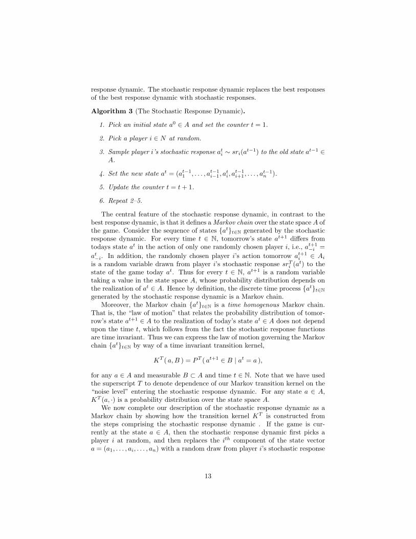
Algorithm 3 (The Stochastic Response Dynamic).

1. Pick an initial state a0 ∈ A and set the counter t = 1.

2. Pick a player i ∈ N at random.

3. Sample player i’s stochastic response ati ∼ sri(at−1) to the old state at−1 ∈

A.

4. Set the new state at = (at−11 , . . . , at−1

i−1, ati, a

t−1i+1, . . . , a

t−1n ).

5. Update the counter t = t + 1.

6. Repeat 2–5.

The central feature of the stochastic response dynamic, in contrast to thebest response dynamic, is that it defines a Markov chain over the state space A ofthe game. Consider the sequence of states {at}t∈N generated by the stochasticresponse dynamic. For every time t ∈ N, tomorrow’s state at+1 differs fromtodays state at in the action of only one randomly chosen player i, i.e., at+1

−i =at−i. In addition, the randomly chosen player i’s action tomorrow at+1

i ∈ Ai

is a random variable drawn from player i’s stochastic response srTi (at) to the

state of the game today at. Thus for every t ∈ N, at+1 is a random variabletaking a value in the state space A, whose probability distribution depends onthe realization of at ∈ A. Hence by definition, the discrete time process {at}t∈Ngenerated by the stochastic response dynamic is a Markov chain.

Moreover, the Markov chain {at}t∈N is a time homogenous Markov chain.That is, the “law of motion” that relates the probability distribution of tomor-row’s state at+1 ∈ A to the realization of today’s state at ∈ A does not dependupon the time t, which follows from the fact the stochastic response functionsare time invariant. Thus we can express the law of motion governing the Markovchain {at}t∈N by way of a time invariant transition kernel,

KT ( a,B ) = PT ( at+1 ∈ B | at = a ),

for any a ∈ A and measurable B ⊂ A and time t ∈ N. Note that we have usedthe superscript T to denote dependence of our Markov transition kernel on the“noise level” entering the stochastic response dynamic. For any state a ∈ A,KT (a, ·) is a probability distribution over the state space A.

We now complete our description of the stochastic response dynamic as aMarkov chain by showing how the transition kernel KT is constructed fromthe steps comprising the stochastic response dynamic . If the game is cur-rently at the state a ∈ A, then the stochastic response dynamic first picks aplayer i at random, and then replaces the ith component of the state vectora = (a1, . . . , ai, . . . , an) with a random draw from player i’s stochastic response

13

function sri(a). Thus conditional upon player i being the chosen player, we candefine the conditional transition kernel KT

i (a,B) for any measurable B ⊂ A,

KTi (a,B) = srT

i ( {bi ∈ Ai : (a−i, bi) ∈ B} | a ).

The unconditional transition kernel KT is then simply a mixture over the con-ditional transition kernels, i.e.,

KT (a,B) =1n

n∑i=1

KTi (a,B). (6)

Thus for a fixed “noise level” T , which recall indexes the level of variabilityof the logit choice probability in the stochastic response dynamic produces aMarkov chain {at}t∈N whose motion is described by the transition kernel KT .

5.4 Convergence to Stationarity

We are now ready to consider the asymptotic behavior of the stochastic re-sponse dynamic. The key feature of this behavior is that it avoids the lack ofconvergence problem of the best response dynamic. To see this, suppose we sim-ulate the stochastic response dynamic for a fixed noise level T . Thus we startthe process at an arbitrary state a0 ∈ A, and grow the process by iterativelydrawing at ∼ KT (at−1, ·). A natural question to ask of such a process, and acentral questions in the study of Markov chains more generally [17], is weatherthe behavior of the random variables at becomes “stable” as t grows large? Inthe case of the stochastic response dynamic, unlike the best response dynamic,we are able to answer this question in the affirmative.

Recall that in the case of the best response dynamic, stability of the process{at}t∈N means that it determinstically converges to a stable point a∗ in A, i.e.,a point a∗ such that if the initial state of the process a0 = a∗, then all thefollowing states of the process at would remain equal to a∗. The stable pointa∗ would thus correspond to a Nash equilibrium. The main problem with thebest response dynamic however is that such a convergence to equilibrium cannotgenerally be assured for most starting values. Further conditions on the shapeof the best response functions are needed to ensure convergence, which are nolonger natural primitives to impose on the game.

In the case of the stochastic response dynamic however, stability of theprocess {at}t∈N means that it converges to a stable probability distribution PT

over A, i.e., a distribution PT such that if the initial state of the process a0

is distributed according to PT , then all the following states of the process at

would remain distributed according to PT . Recall from Markov chain theorythat if the initial state a0 of the chain {at}t∈N is generated according to someprobability measure Q0 over A, then marginal probability distribution Qt of at

is given inductively by

Qt(B) =∫

KT (x, B)Qt−1(dx),

14

for measurable B ⊂ A.The key feature of the stochastic response dynamic is that for any choice

of Q0, the marginal distributions Qt converges strongly (i.e. in total variationnorm) to a unique limiting probability measure7 PT . This follows from thefact, as we shall show, that the Markov chain associated with the transitionkernel KT satisfies strong ergodic properties. In particular, the Markov chaindefined by KT is positive, irreducible, and Harris recurrent [17]. From theseproperties, it follows that for a sufficienctly large number of iterations jT ∈ N,the state of the process ajT will be distributed as approximately (for arbitrarysmall approximation error in total variation norm) PT , i.e.,

ajT ∼ PT . (7)

We refer to the distribution PT as the equilibrium of the stochastic responsedynamic. Moreover the equilibrium distribution PT will also be a stable orinvariant probability distribution for the process {at}t∈N in the sense definedabove.

Thus for any game in our class, the stochastic response dynamic solves theinstability problem of the best response dynamic by way of simulating a Markovchain with transition kernel KT that has an equilibrium distribution PT . How-ever the fact that it solves the lack of stability problem of the best responsedynamic does not yet mean it necessarily solves our problem, which is to findNash equilibrium.

The equilibrium distribution PT of the stochastic response dynamic doesnot yet bear any obvious relation to the Nash equilibria of the underlying game.However our main result shows that for our class G of games, which we conjec-ture satisfies the natural game theoretic condition that we call Nash connected-ness, PT is in fact related to the Nash equilibrium of the underlying game in acomputationally quite relevant way, which we explain next.

5.5 Convergence to Nash

Thus far we have considered the stochastic response dynamic for only a fixednoise level T . We have argued that for each fixed noise level T > 0, the stochasticresponse dynamic with kernel KT has a unique equilibrium distribution PT .For T infinitely large, which corresponds to the stochastic response dynamicbecoming infinitely noisy, the equilibrium distribution PT becomes maximallyvariant, and approaches a uniform distribution over the state space A.

However as the “noise” in the stochastic response dynamic gets smaller andsmaller, the sequence of equilibrium distributions PT converges in distribitionto a limit distribution P . Our main result is that for games in G that furthersatisfy a condition we call Nash Connectedness, which we conjecture holds truefor all games in G, and prove holds true for two player games in G, the supportof P consits entirely of Nash equilibria. Thus for small T , the equilibrium

7We maintain the T index as reminder that this limiting measure will depend on the noiselevel T of the stochastic response dyanamic.

15

distribution PT becomes increasingly concentrated over the the Nash equilibriastates of the game. Thus if we produce a draw from the distribution PT forsmall T , the probability that this draw if further than any epsilon from a Nashequilibrium goes to zero as T goes to zero.

In light of the main result, computing Nash equilibrium via the stochasticresponse dynamic becomes clear. Start at some large T > 0, and simulate thestochastic response dynamic. The subsequent values at

T for t = 1, 2, . . . , etc ofthe process can then be approximately regarded as a sample from its equilibriumdistribution PT . For large T , this sample will resemble a uniform distributionover A. After some pre-specified number of iterations (call it the thresholdnumber of iterations), decrease the noise level T by some factor, and repeat.

As T gets smaller, the equilibrium distribution PT , and hence the simulatedvalues at

T becomes more concentrated over the Nash equilibrium states of thegame. Eventually, the process will get “stuck” in a state a∗∗ ∈ A for which nocandidate responses are accepted after the threshold number of attempts. Thisstate a∗∗ is by definition an approximate Nash equilibrium since no player iswilling to move under the stochastic response dynamic.

This process of learning Nash equilibrium, which combines the basic stochas-tic response dynamic with a “noise reduction” schedule, bears a resemblance to“annealing” methods in physics. Such annealing methods first heat up a physi-cal system so as to make its particles move around rapidly, which is the analogueof the equilibrium distribution of the stochastic response dynamic. The systemis then cooled, i.e., made less noisy, so as to bring the system to its equilib-rium motionless or crystal state – which is analogous to the stochastic responsedynamic coming to rest on a Nash equilibrium.

6 Where Does it Come From and Why Does itWork

We have just made some bold claims about the behavior of the stochastic re-sponse dynamic for our class of games G. In this section we seek to presentthe basic idea that motivates thee stochastic response dynamic as a new wayto learn and compute equilibrium. This motivation provides proof of its func-tionality in a somewhat more specialized setting than the entire class G. Wethen lay the foundations for the generalizability of the proof to the entire classof games G. Finally, we conclude with computational experiments.

The fundamental new idea is to recognize that strategic games bear a verynatural relationship to conditionally specified probability models. A condition-ally specified probability model is a system of conditional probability densityfunctions pi( xi | x−i ) for i = 1, . . . n that describes the joint distribution of arandom vector (X1, . . . , Xn). We now show how it is possible to transform anygiven strategic game (even though we are only interestd in games in G) intosuch a system of conditional probability density functions (conditional pdf’sfor short) without “changing” the game (i.e., preserving the Nash equilibria).

16

Using this transformation, the motivation for the stochastic response dynamicbecomes clear.

6.1 Games as Conditional Probabilities

The first step is to recognize that for the purposes of Nash equilibrium, thevariation of each utility function ui over the entire space A is not significant,but only the variation of ui over own actions Ai for each fixed profile a−i of theother players’ actions. It then becomes natural to speak of each player havinga conditional utility function ui( ai | a−i) = ui(a−i, ai) over the axis Ai foreach fixed profile a−i ∈ A−i of other player actions. Thus instead of viewinga game as n utility functions, we can equivalently think of it as a system of nconditional utility functions ui( ai | a−i ). A Nash equilibrium a∗ ∈ A is a pointthat maximizes each player’s conditional utility function,

a∗i = arg maxai∈Ai

ui( ai | a∗−i ).

However once we express the game as a system of conditional utility func-tions, it begins to “look” very similar to a situation from standard probabilitytheory. We will make this similarity apparent by first normalizing each condi-tional utility function ui( ai | a−i ) to be strictly positive and integrate to oneas a function of ai. One way of doing this is using the tranformation

pTi ( ai | a−i ) ∝ exp

(ui( ai | a−i )

T

)(8)

= cTa−i

exp(

ui( ai | a−i )T

)The parameter T is a positive real number that has the same interpretation asthe noise parameter in the stochastic response dynamic, but we shall make thisconnection later. For now, notice only that a small T makes the conditionalpdf pT

i more “peaked” around its mode (pTi is unimodal because of the strict

quasiconcavity assumption made of games in G), and for large T , pTi becomes

flat (uniform) over A.Notice that there is a constant cT

a−iof proportionality (depending on both

T and a−i) needed so that the resulting normalized conditional utility functionpT

i ( ai | a−i ) satisfies the property of integrating to one over Ai. At no point dowe ever need to compute this constant, but it is useful to be aware that it existsgiven the assumptions we have made about the game (recall A is compact andthus a normalization constant exists).

The next step is to notice that normalizing the conditional utility functionsdoes not change Nash equilibrium. That is, a∗ ∈ A also satisfies

a∗i = arg maxai∈Ai

pTi ( ai | a∗−i ). (9)

Thus we have gone from n utility functions ui to n conditional utility func-tions ui( ai | a−i ) to n normalized conditional utility functions pT

i ( ai | a−i ).

17

The advantage to us of working with pTi ( ai | a−i ) is that it not only provides

an equivalent model of the original strategic game, but it also serves as a con-ditionally specified probability model.

That is, each pTi ( ai | a−i ) can be interpreted as a conditional probability

density function, since as a function of ai, it is strictly positive and integratesto one. Thus one can postulate the existence of a vector of random variables(X1, . . . , Xn) having support A = A1×· · ·×An, and whose conditional distribu-tions are described by the conditional probability density functions pT

i ( ai | a−i ).We also observe that the conditional pdf’s pT

i ( ai | a−i ) are equal to the quantalresponse functions of McKelvey and Palfrey [21] (which are distinct from ourstochastic response functions), but generalized to continuous action sets.

The system of conditional pdf’s pTi ( ai | a−i ), or quantal response func-

tions, conditionally specifies a probability model for a random vector X =(X1, . . . , Xn) having support A = A1×· · ·×An. That is, the system pT

i ( ai | a−i )of conditional pdf’s specifies all the conditional distributions of the random vec-tor (X1, . . . , Xn).

6.2 Compatibility

When we are given the n utility functions ui that define a game, there is no gen-eral way to combine them into a single function u over A whose characteristicsbear any obvious relation to the Nash equilibria of the game. The closest thingwe have to such a method of combining the utility functions is the Calculusapproach, which forms the system of first order conditions and associates Nashequilibria with the roots of the system.

However the key innovation in thinking of a game in terms of the conditionalpdf’s pT

i ( ai | a−i ) is that it allows us to use tools from probability to combinethe utilities. In particular, let us assume that the system of conditional pdf’spT

i ( ai | a−i ) that we derive from G are compatible. That is, assume thatthere exists a joint pdf pT (a1, . . . , an) that has conditional distributions equalto pT

i ( ai | a−i ). More formally, the conditional pdf’s pTi are compatible if there

exists a real valued function qt over A such that for any i, and any a−i ∈ A−i,

pTi ( ai | a−i ) = Ka−iq

T (a1, . . . , an), (10)

for a constant Ka−i . If such a function exists, then it is clear that the jointpdf pT having pT

i ( ai | a−i ) as its conditional pdfs is given by pT (a1, . . . , an) =cqT (a1, . . . , an) for a constant of proportionality that enables pT to integrate to1. Thus (10) expresses the usual relation that the joint distribution of a randomvector (X1, . . . , Xn) is proportional to its conditionals. By a basic theorem inprobability theory, known as the Hammersley-Clifford Theorem [9], if such ajoint distribution pT exists, then under mild regularity conditions, which aremet by our conditionals pT

i because they have full support Ai, this joint isuniquely determined.

In fact, for our conditional system, if such a joint pT exists for a single T ,say T = 1, it follows that a joint pT will exist for all T > 0. We now state thisas a lemma.

18

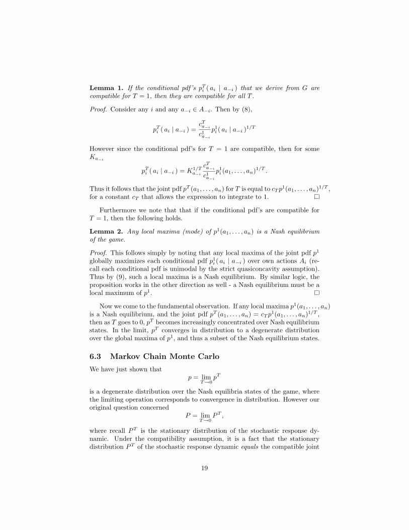
Lemma 1. If the conditional pdf’s pTi ( ai | a−i ) that we derive from G are

compatible for T = 1, then they are compatible for all T .

Proof. Consider any i and any a−i ∈ A−i. Then by (8),

pTi ( ai | a−i ) =

cTa−i

c1a−i

p1i ( ai | a−i )1/T

However since the conditional pdf’s for T = 1 are compatible, then for someKa−i

pTi ( ai | a−i ) = K1/T

a−i

cTa−i

c1a−i

p1i (a1, . . . , an)1/T .

Thus it follows that the joint pdf pT (a1, . . . , an) for T is equal to cT p1(a1, . . . , an)1/T ,for a constant cT that allows the expression to integrate to 1.

Furthermore we note that that if the conditional pdf’s are compatible forT = 1, then the following holds.

Lemma 2. Any local maxima (mode) of p1(a1, . . . , an) is a Nash equilibriumof the game.

Proof. This follows simply by noting that any local maxima of the joint pdf p1

globally maximizes each conditional pdf p1i ( ai | a−i ) over own actions Ai (re-

call each conditional pdf is unimodal by the strict quasiconcavity assumption).Thus by (9), such a local maxima is a Nash equilibrium. By similar logic, theproposition works in the other direction as well - a Nash equilibrium must be alocal maximum of p1.

Now we come to the fundamental observation. If any local maxima p1(a1, . . . , an)is a Nash equilibrium, and the joint pdf pT (a1, . . . , an) = cT p1(a1, . . . , an)1/T ,then as T goes to 0, pT becomes increasingly concentrated over Nash equilibriumstates. In the limit, pT converges in distribution to a degenerate distributionover the global maxima of p1, and thus a subset of the Nash equilibrium states.

6.3 Markov Chain Monte Carlo

We have just shown thatp = lim

T→0pT

is a degenerate distribution over the Nash equilibria states of the game, wherethe limiting operation corresponds to convergence in distribution. However ouroriginal question concerned

P = limT→0

PT ,

where recall PT is the stationary distribution of the stochastic response dy-namic. Under the compatibility assumption, it is a fact that the stationarydistribution PT of the stochastic response dynamic equals the compatible joint

19

pT . This is because the stochastic response dynamic is nothing more than aform of Markov Chain Monte Carlo when the system of conditional pdf’s iscompatible.

Markov Chain Monte Carlo is concerned with the construction of a MarkovChain M over a given state space S whose equilibrium distribution is equal tosome given probability distribution of interest π over S. One of the first MarkovChain Monte Carlo algorithms to emerge was the Metropolis algorithm [16], ormore precisely the “variable at a time” Metropolis algorithm [2]. If the statespace can be expressed as a product S = S1×· · ·×Sn, then the Metropolis algo-rithm shows how to construct a Markov chain M whose equilibrium distributionis π. It constructs this chain by using the information contained conditionalsdistributions π( si | s−i ).

In terms of our state space A, and our joint pdf pT (a1, . . . , an) over A thatwe derived from the conditional pdf’s pT

i ( ai | a−i ) and the compatibility as-sumption, the Metropolis algorithm provides a recipe for constructing a Markovchain whose equilibrium distribution is pT . This recipe is as follows:

Algorithm 4 (Metropolis Algorithm for Games).

1. Start the process at any state a0 ∈ A and set the counter t = 1.

2. Pick a player i ∈ N at random.

3. Draw a candidate a′i action from a uniform distribution over Ai.

4. Set the new state at+1 = (at1, . . . , a

ti−1, a

′i, a

ti+1, . . . , a

tn). with probability

Pi(a′i, at) =

1

1 +(

pTi ( at

i|at−i )

pTi ( a′i|at

−i )

) . (11)

and set at+1 = at with probability 1−Pi(a′i, at).

5. Update the counter t = t + 1.

6. Repeat 2–4.

The acceptance probability expressed in (11) is one version of the Metropoliscriterion. The remarkable feature of the Metropolis algorithm is that the onlyinformation it uses about the joint distribution pT is conveyed by the Metropoliscriterion. This has proved powerful in a range of applications for which somejoint distribution π over a state space S = S1×· · ·×Sn needs to be studied, butπ may only be known up to its set of conditional distributions πi( si | s−i ) fori = 1, . . . , n, and each πi may only be known up to a constant of proportionality.

If we rewrite the Metropolis criterion in terms of the underlying utility func-tions of our game by expanding the definition of pT

i given in (8), it yields

11 + exp[−(ui(at

−i, a′i)− ui(at

−i, ati))/T ]

. (12)

20

But (12) this is nothing more than the probability of accepting a candidateresponse in (3) under the stochastic response dynamic. Thus the Metropolisalgorithm for games and the stochastic response dynamic are the same.

Hence under the compatibility assumption, the standard results on theMetropolos algorithm allow us to conclude that the equilibrium distributionof the stochastic response dynamic PT equals the compatible joint distributionpT . Thus it follows from lemma 2 that

limT→0

PT ,

is a degenerate distribution over Nash equilibria states of the game, which isprecisely the main result we wished to establish.

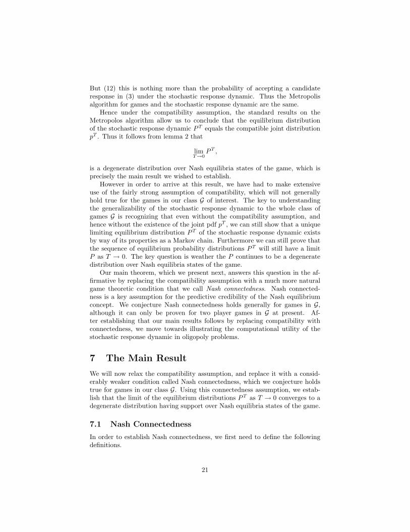
However in order to arrive at this result, we have had to make extensiveuse of the fairly strong assumption of compatibility, which will not generallyhold true for the games in our class G of interest. The key to understandingthe generalizability of the stochastic response dynamic to the whole class ofgames G is recognizing that even without the compatibility assumption, andhence without the existence of the joint pdf pT , we can still show that a uniquelimiting equilibrium distribution PT of the stochastic response dynamic existsby way of its properties as a Markov chain. Furthermore we can still prove thatthe sequence of equilibrium probability distributions PT will still have a limitP as T → 0. The key question is weather the P continues to be a degeneratedistribution over Nash equilibria states of the game.

Our main theorem, which we present next, answers this question in the af-firmative by replacing the compatibility assumption with a much more naturalgame theoretic condition that we call Nash connectedness. Nash connected-ness is a key assumption for the predictive credibility of the Nash equilibriumconcept. We conjecture Nash connectedness holds generally for games in G,although it can only be proven for two player games in G at present. Af-ter establishing that our main results follows by replacing compatibility withconnectedness, we move towards illustrating the computational utility of thestochastic response dynamic in oligopoly problems.

7 The Main Result

We will now relax the compatibility assumption, and replace it with a consid-erably weaker condition called Nash connectedness, which we conjecture holdstrue for games in our class G. Using this connectedness assumption, we estab-lish that the limit of the equilibrium distributions PT as T → 0 converges to adegenerate distribution having support over Nash equilibria states of the game.

7.1 Nash Connectedness

In order to establish Nash connectedness, we first need to define the followingdefinitions.

21

Definition 1. For a game G, the relation > over A is defined such that aj > ak

iff for some player i, ak−i = aj

−i and ui(ak) > ui(aj).

Thus aj > ak iff and only if a single player changes his action betweenaj and ak, and this player improves his utility. We can thus say that aj andak are related by a single player improvement. A subset B ⊂ A of the jointaction space of the game is said to be closed under single player improvementsif for any a ∈ B, b ∈ A and b > a implies b ∈ B. That is, for any statein B, a single player improvement of that state is also contained in B. Thuswe can alternatively define Nash equilibrium a∗ as simply a singelton set {a∗}that is closed under single player improvements (i.e. the set of single playerimprovements from Nash equilibrium is the empty set).

Definition 2. A chain γ in G is a sequence {a0, a1, . . . , an} in A such thatak > ak−1 for k = 1, . . . , n.

Definition 3 (Nash Connectedness). A game G possessing a pure strategy Nashequilibrium is Nash connected if for any ε > 0, and any initial state a0 ∈ A,there exists a chain γ = {a0, . . . , an} such that an is in the epsilon open ballcentered at some Nash equilibrium a∗ ∈ A.

Whereas compatibility was clearly a somewhat artifical assumption to im-pose on our class G, Nash connectedness is an entirely natural assumption toimpose. We conjecture that for games in G, connectedness will be satisfied. Atpresent, the connectedness assumption has only been proved for 2 player gamesin G by way of an adaptation of theorem 2 in [6]. The author is at present devel-oping a proof for the general case based on the Lefschetz fixed point theorem.

One motivating idea to see the naturalness of connectedness is to thinkwhat it would mean for it to fail. Failure of connectedness would actuallyundermine the predictive value of Nash equilibrium. In order to make thispoint, we establish the following result.

Theorem 1. For a continuous game G that has a Nash equilibrium a∗, Nashconnectedness fails if and only if there exists a closed subset B ⊂ A of the jointaction space, which does not contain a Nash equilibrium and is closed undersingle player improvements.

Proof. Obviously if such a set existed, then Nash connectedness fails for anypoint b ∈ B, since any Nash equilibrium has an epsilon ball around it that doesnot intersect B, and thus no chain from within B can enter any of these epsilonballs.

The other direction works as follows. Suppose Nash connectedness fails ata point a0. Then build the following sets inductively. Let S0 = {a0}. LetSn = {a ∈ A : a > b for some b ∈ Sn−1}. Then let S∞ be the countable unionover the Sn sets for n = 1, 2, . . . , etc, and S̄ be the closure of S∞. It followsthat S̄ is closed (by construction). Moreover, since Nash connectedness is beingassumed to fail, S̄ does not contain a Nash equilibrium. We wish to show thatS̄ satisfies the property of B in the proposition, namely, it is closed under singleplayer improvements.

22

Suppose that S̄ was not closed under single player improvements, i.e. thereis some point x ∈ S̄ that has a single player improvement z ∈ A not in S̄. Thenthe failure must occur at a limit point x of S∞ because otherwise x would becontained in an Sn for finite n, and thus z would be in Sn+1.

Let us say without loss of generality that state z is a single player improve-ment for player i from state x.Thus we have that x = (xi, x−i) and z = (zi, x−i)for some zi not equal to xi. However since x is a limit point of S∞, then thereis a sequence of points xn for n = 1, 2, . . . , etc in S∞ converging to x. Howeverby definition of z, ui(zi, x−i) > ui(xi, x−i), and thus for xn close to x it followsby continuity of ui that ui(zi, x

n−i) > ui(xn

i , xn−i). But this means that (zi, x

n−i)

is in S∞ for all large n. Thus the limit (zi, x−i) of (zi, xn−i) is in S̄ since S̄ is

the closure of S∞. But this contradicts our assumption that z = (zi, x−i) wasnot in S̄. Thus it must be in S̄.

Here then is the pathology. Nash connectedness is equivalent to the existenceof a closed set B ⊂ A, which is strictly bounded away from any Nash equilibria,but would be as potent a solution for the game as any Nash equilibrium a∗.That is, if someone announced to the players that the outcome of the game willlive B, then this prediction would be self reinforcing because no player wouldwant to deviate from B, i.e., B is closed under single player improvements.This undermines the predictive value of Nash equilibrium - there is no a priorireason to assume the outcome of the game will be in the set {a∗} for some Nashequilibrium a∗, or B, which is bounded away from any Nash equlibrium. Bothsets satisfy the same rationality requirements of being closed under single playerimprovements, i.e., no player has the incentive to deviate from the solution.

We conjecture that for games in G, i.e. quasiconcave game for which equi-librium is known to exist, this pathology cannot arise. At present the result isonly known for 2 player games in G. The proof of this follows by way of anadaptation of Theorem 2 in [6]. The author is currently developing a proof forthe general case based on an application of the Lefschetz fixed point theorem(which allows for proving fixed point results without requring the domain of theunderlying function be convex).

7.2 Main Theorem

Theorem 2. For games in G, if Nash connectedness is satisfied, then the equi-librium distribution PT converges in distribution to a degenerate distributionover Nash equilibria states of the game as the noise T → 0.

Proof. We present the logical flow of the proof, and for the sake of length, themathematical details are left to the references. Without compatibility, we needto first show that an invariant probability measure PT for the Markov kernelKT exists. Continuity of the utility functions ui allows us to conclude that thethe kernel KT for any T > 0 will will be define a weak Feller chain [17]. Sinceour state space A is compact and by property of Feller chains, we can assure a

23

fixed point PT for the kernel KT exists, which will be an invariant probabilitymeasure for the process.

Secondly we need to show that for T > 0, PT is the unique invariant mea-sure, and the chain will strongly converge to PT , i.e. in total variation norm.This follows from the irreducible and aperiodic behavior of the stochastic re-sponse dynamic. From any one point in the state space, the stochastic responsedynamic can with positive probability travel to any other open set in a finitenumber of steps, which means it is irreducible. Moreover, there is a strictlypositive probability that starting from any state, we can enter any open set ofA in n iterations of the chain (where n is the number of players). Thus the chainsatisfies a strong recurrency condition known as Harris recurrence. Also, sincethere is always some positive probability of staying at the current state afterone iteration (i.e. rejecting the candidate response), the chain is also aperiodic.By standard ergodic theorems for irreducible Harris recurrent chains that admitinvariant measures, found in [17], PT is the equilibrium distribution, i.e., theunique invariant probability measure for KT to which the marginal distribu-tions of the process converge strongly. We also have that PT can be describedby a density function, i.e. PT is absolutely continuous with respect to Lesbeguemeasure, which follows from irreducibility.

Now we wish to understand what happens to PT as T → 0. First werecognize the kernel KT has a limit K as T → 0. The underlying stochasticresponse functions of this limiting kernel K consist of a player randomly pickinga new action and changing to this action if it weakly improves utility. This kernelK also defines a weak Feller chain based on the continuity of the ui. Clearly aDirac (delta) measure concentrated over a Nash equilibrium state is an invariantprobability measure for K. i.e., if we start at Nash, then under K, we stay there.

Through the Nash connectedness assumption, we can show that the onlyinvariant probability mesures of the limiting kernel K are the Nash equilibriaDirac (delta) measures and their convex mixtures. If there existed any otherinvariant measure, then this would imply that there exists an ergodic invari-ant probability measure of K that puts positive probability on an open set notcontaining any Nash equilibria. By Nash connectedness, this invariant prob-ability measure must contain a Nash equilibrium a∗ in its support. Howeverthis would imply that the support of one ergodic probability invariant measurestrictly contained the support of another ergodic invariant probability measure(namely the support of the Dirac measure concentrated at a∗), which is im-possible for Feller chains on compact metric spaces as can be shown from themain result in Chapter 4 of [24]. Thus the Dirac measures concentrated at Nashequilibria states and their convex combinations are the only invariant measuresfor K. Said another way, every invariant measure measure of K has a supportconsisting entirely of Nash equilibria.

However K will of course not be irreducible, which is why we don’t runthe stochastic response dynamic at K but rather use noise T > 0. However astandard result from [5] shows that the sequence of equilibrium distributionsPT for KT converge weakly (in distribution) to an invariant distribution of thelimiting kernel K. But all invariants of K are supported over Nash equilibria

24

staes. This would end the proof.

8 Computational Examples – Cournot Equilib-rium

Many problems in industrial organization are formulated quite naturally as N -player games. In this section, the behavior of the stochastic response dynamic isillustrated for a few simple cases of the the Cournot oligopoly model. Follow upwork to this primarily theoretical paper uses the stochastic response dynamicto perform more substantive economic analysis, i.e., merger analysis.

The Cournot oligopoly models the strategic interactions that occur amongN firms who each produce the same good. If each firm i chooses an amount qi

to produce, then the total quantity Q = q1 + q2 + · · ·+ qN produced determinesthe price p of the good via the inverse market demand p(Q). Furthermore, eachfirm i incurs a cost ci(qi) to produce its chosen amount qi. The choice eachfirm i faces is strategic because the profit πi(qi, q−i) = p(Q)qi− ci(qi) it receivesfrom producing qi depends on the quantities q−i produced by the other firms.Thus as a game, the Cournot oligopoly consists of:

1. N firms

2. An action set Ai = [0, q̄] for each firm i from which it chooses an amount qi

to produce. The upper limit q̄ on each firm’s actions set Ai is understoodeither as a capacity limit, or as the quantity above which the price on themarket for the good is zero.

3. A utility function ui(qi, q−i) for each firm i that equals its profit πi(qi, q−i) =p(Q)qi − ci(qi) from having produced qi and its competitors having pro-duced q−i.

Assuming different forms of market demand p(Q) and firm specific costsci(qi) leads to a variety of possible Cournot oligopoly games. The stochasticresponse dynamic as a computational tool is now illustrated using some specificforms that are also easily solvable by means of the more traditional Calculusapproach. Our purposes in these illustrations is to just convey an image ofthe stochastic response dynamic in practice – thus we have kept the examplesintentionally fairly simple.

For each case of Cournot considered, the definition of the game is given,followed by the solution known by way of traditional technique, and then thestochastic response dynamic output. The algorithm is run at a starting noiselevel of 1, and reduced by .01 every 1000 iterations until a noise level is reachedsuch that no candidate actions are accepted. The state of simulation in the finalstate is rounded to two decimal places is taken to be the computed solution ofthe game. We see that for each case, we successfully reproduces the knownCournot solutions.

25

8.1 Linear Demand No Cost Cournot

1. 2 Players

2. A1 = [0, 1] and A2 = [0, 1]

3. π1(q1, q2) = q1(1− (q1 + q2)) and π2(q1, q2) = q2(1− (q1 + q2))

The Nash equilibrium of the game is q∗1 = 1/3 and q∗2 = 1/3.The stochastic response dynamic resulted in the following simulation:

0 4000 8000

0.0

0.2

0.4

0.6

0.8

1.0

Player 1

Iteration

A1

0 4000 8000

0.0

0.2

0.4

0.6

0.8

1.0

Player 2

Iteration

A2

The simulation stopped in the state q̂1 = 0.33 and q̂2 = 0.33.

Stackelberg Cournot

1. 2 Players

26

2. A1 = [0, 1000] and A2 = [0, 1000]

3. πi(q1, q2) = qi(100e−(1/10)√

q1+q2) for i = 1, 2.

The Nash equilibrium of the game is q∗1 = 800 and q∗2 = 800 [15].The stochastic response dynamic resulted in the following simulation.

0 40000 80000

020

040

060

080

010

00

Player 1

Iteration

A1

0 40000 80000

020

040

060

080

010

00

Player 2

Iteration

A2

The simulation stopped in the state q̂1 = 800.03 and q̂2 = 799.98.

Hard Cournot

This is an example of a more challenging Cournot computation. It is outsidethe realm of the previous examples in that it cannot be done by hand, and hasbeen used for demonstrating numerical techniques for finding equilibrium underthe traditional approach.

27

In this case, there are 5 firms. Each has a cost function

Ci(qi) = ciqi + βi/(βi + 1)5−1/βiq(βi+1)/βi

i ,

for firm i = 1, 2, 3, 4, and 5. Furthermore the industry demand curve for theircommon product is

p = (5000/Q)1/1.1.

The paramters of the 5 firm specific cost functions are given in the followingtable:

firm i ci βi

1 10 1.22 8 1.13 6 1.04 4 0,95 2 0.8

The Nash equilibrium of this game has been numerically found [14] to beapproximately

(q∗1 = 36.93, q∗2 = 41.82, q∗3 = 43.70, q∗4 = 42.66, q∗5 = 39.18).

The stochastic response dynamic resulted in the following output:

28

0 2000 4000 6000 8000 10000

030

Player 1

Iteration

A1

0 2000 4000 6000 8000 10000

030

Player 2

Iteration

A2

0 2000 4000 6000 8000 10000

030

Player 3

Iteration

A3

0 2000 4000 6000 8000 10000

030

Player 4

IterationA

4

0 2000 4000 6000 8000 10000

030

Player 5

Iteration

A5

The simulation stopped in the state

(q̂1 = 36.92, q̂2 = 41.87, q̂3 = 43.71, q̂4 = 42.66, q̂5 = 39.18).

9 Capacity Constraints

The preceding examples illustrated the use of the stochastic response dynamicas a computational tool for a variety of Cournot oligopoly models. However allof these games were just as easily solvable by traditional “Caclulus” means. Wenow illustrate a problem that becomes “harder” for the Calclus approach butdoes not disturb the stochastic response dynamic.

A game in which the Calculus approach cannot proeed in the usual way oc-curs when the firms supplying a market have capacity constraints on the amountthey can produce. Capacity constraints are an empirically relevant fact of in-dustrial life, and thus are important to include in an oligopoly model. However

29

capacity constraints cause a lack of differentiability in the utility functions toarise, thus violating the necessity assumption on the payoffs imposed by theCalculus approach (the necessity assumption was discussed in section 4).

Froeb et al. [7] have recently explored the problem of computing equilibriumin the presence of capacity constraints. They use a differentiated productsBertrand oligopoly. That is, an oligopoly model where firms are price settersrather than quantity setters, and the firms not homogenous.

To see the problem introduced by capacity constraints, let qi be the amountsupplied by each firm i, which is a function of both own price pi and the pricesof the other firms p−i. If firm i faces no capacity constraints, then its profitfunction is

ui( pi, p−i ) = piqi(pi, p−i)− ci(qi(pi, p−i)).

The best response bri(p) of firm i to a profile of prices p = (pi, p−i) is chosen soas to satisfy its first order condition, i.e., firm i solves the equation

d

dpiui(pi, p−i) = 0.

However if firm i faces a capacity constraint ki on the amount it can produce,then the profit function becomes

ui( pi, p−i ) = pi min(qi(pi, p−i), ki)− ci(min(qi(pi, p−i), ki)).

Depending on the profile of prices p, the constrained best response bri(p) offirm i is the solution to one of two potential equations. If the unconstrainedbest response p′i results in a demand qi that does not exceed capacity ki, theconstrained best response is also p′i, and the capacity constraint has no effect.However if the unconstrained best response p′i results in a demand qi that ex-ceeds capacity ki, then the constrained best response p′′i is set so as to solve theequation

qi(pi, p−i)− ki = 0.

This situation is shown graphically below.

30

pi

g i(

p i |

p −i )

ConstrainedUnconstrained

Firm i’s Conditional Profit Function

Thus each player may not be solving its first order condition in equilibrium,which forces one to modify the standard Calculus approach to computation.

However it is easy to imagine that the stochastic response dynamic wouldhave an even easier time with the constrained problem than with the uncon-strained problem. This follows from looking at the graph of the profit functionfor the capacity constrained producer. The capacity constraint introduces akink into the profit function of each firm with respect to own action. Thus inequilibrium, any firm that is capacity constrained also has a profit function thatis more “peaked” at the maximum than in the unconstrained case. In terms ofthe equilibrium distribution of the stochastic response dynamic PT , which be-comes increasingly centered over Nash equilibrium as T → 0, the “mode” of PT

will become sharper via the capacity constraint. Thus we expect the stochasticresponse dynamic to get stuck in equilibrium more readily under constraintsthan without constraints.

To illustrate, the stochastic response dynamic was run on the Bertrand

31

oligopoly model employed in Froeb et al. [7]. The stochastic response dynamicresulted in the following output, first for the unconstrained case, and then forthe constrained case. As can be seen, the output for the constrained case showsthe simulation getting “stuck” in a mode faster than for the unconstrained case.

0 5000 15000

0.0

0.5

1.0

1.5

2.0

2.5

3.0

Player 1

Iteration

A1

0 5000 15000

0.0

0.5

1.0

1.5

2.0

2.5

3.0

Player 2

Iteration

A2

0 5000 15000

0.0

0.5

1.0

1.5

2.0

2.5

3.0

Player 3

Iteration

A3

Unconstrained Oligopoly

32

0 5000 15000

0.0

0.5

1.0

1.5

2.0

2.5

3.0

Player 1

Iteration

A1

0 5000 15000

0.0

0.5

1.0

1.5

2.0

2.5

3.0

Player 2

Iteration

A2

0 5000 150000.

00.

51.

01.

52.

02.

53.

0

Player 3

Iteration

A3

Constrained Oligopoly

10 Conclusion

In this paper we have shown a new approach to learning and computing Nashequilibrium in continuous games that abandons the methods and assumptionsof the traditional Calculus driven approach. The stochastic response dynamicis unlike the Calculus based approach to finding Nash equilibrium in two im-portant respects. First the stochastic response dynamic is decentralized, andthus corresponds to a formal model of learning in economic environemnts. Sucha learning model provides a solution to equilibria selection in the presence ofmultiple equilibria in structural game theoretic models. Second, the stochasticresponse dynamic converges (probabilistically) to Nash over the general class ofgames G of interest without making any differentiability assumptions, assum-ing only that G satisfies the natural game theoretic condition we term Nashconnectedness. We conjecture Nash connectedness holds true for G, but only

33

are able to prove for 2 player games in G at present. An important basis forunderstanding why the stochastic response dynamic would work in the mannerdescribed was the link we established between strategic games and condition-ally specified probability models. Essentially this link to probability modelsmotivates the stochastic response dynamic. After establishing the main conver-gence properties of the stochastic response dynamic, we proceeded to illustrateits computational behavior on a variety of oligopoly games, including those inwhich standard differentiability assumptions are not met and thus the Calculusapproach encounters difficulty. The computational behavior conforms to out ex-pectations. Future is work is underway towards establishing Nash connectednessfor the entire class of games G by way of the Lefschetz fixed point theorem.

References

[1] S.P. Brooks and B.J.T. Morgan. Optimisation using simulated annealing.The Statistician, 44:241–257, 1995.

[2] Stephen P. Brooks. Markov chain Monte Carlo method and its application.The Statistician, 47:69–100, 1998.

[3] Augustine Cournot. ”Researches into the Mathematical Principles of theTheory of Wealth”. London, Hafner, ”1838”.

[4] G Debreu. Existence of Competitive Equilibrium, volume 2, chapter 15.North-Holland, 1982.

[5] S. R. Foguel. The Ergodic Theory of Markov Processes. Van NostrandReinhold, New York, 1969.

[6] James W. Friedman and Claudio Mezzetti. Learning in games by randomsampling. Journal of Economic Theory, 98(1):55–84, 2001.

[7] L. Froeb, S. Tschantz, and P. Crooke. Bertrand competition with capac-ity constraints: Mergers among parking lots. Journal of Econometrics,Forthcoming.

[8] D. Fudenberg and J. Tirole. Game Theory. MIT Press, 1996.

[9] S. Geman and D. Geman. Stochastic relaxation, gibbs distributions, andthe bayesian restoration of images. IEEE Transactions on Pattern Analysisand Machine Intelligence, 6:721–741, 1984.

[10] W. R. Gilks, S. Richardson, and D. J. (Ed) Spiegelhalter. Markov ChainMonte Carlo in Practice. Chapman & Hall, 1998.

[11] J.C. Harsanyi. ”games with randomly distributed payoffs: A new ratio-nale for mixed-strategy equilibrium points. Internaional Journal of GameTheory, 2:1–23, 1973.

34

[12] Sergiu Hart and Andreu Mas-Colell. Uncoupled dynamics do not lead tonash equilibrium. American Economic Review, 93(5):1830–1836, December2003.

[13] K Judd. Numerical Methods in Economics. MIT Press, 1998.

[14] C. Kolstad and L. Mathiesen. Computing cournot-nash equilibrium. Op-erations Research, 1991.

[15] S. Martin. Advanced Industrial Economics. Blackwell, 1993.

[16] N. Metropolis, A. Rosenbluth, M. Rosenbluth, A. Teller, and E. Teller.Equation of state calculation by fast computing machines. Journal ofChemical Physics, 21:1087–1092, 1953.

[17] S. Meyn and R. Tweedie. Markov Chains and Stochastic Stability. Springer-Verlag, London, 1993.

[18] Roger B. Myerson. Game Theory: Analysis of Conflict. Havard UniversityPress, Cambridge, Massachusetts, 1991.

[19] M.J. Osborne and A. Rubinstein. A Course in Game Theory. MIT Press,1994.

[20] David C. Parkes and Lyle Ungar. Learning and adaption in multiagentsystems. In Proc. AAAI’97 Multiagent Learning Workshop, Providence,USA, 1997.

[21] M. Richard and T. Palfrey. Quantal response equilibria for normal formgames. Games and Economic Behavior, 10:6–38, 1995.

[22] J. Tirole. The Theory of Industrial Organization. MIT Press, 1988.

[23] Kenneth E. Train. Discrete Choice Methods with Simulation. CambridgeUniversity Press, 2003.

[24] Radu Zahraopol. Invariant Probabilities of Markov-Feller Operators andtheir Supports. Birkhauser Verlag, 2005.

35