the study of scale formation in oil reservoir …eprints.utm.my/id/eprint/5802/1/75224.pdf ·...

THE STUDY OF SCALE FORMATION IN OIL RESERVOIR DURING WATER

INJECTION AT HIGH-BARIUM AND HIGH-SALINITY FORMATION WATER

AMER BADR MOHAMMED BIN MERDHAH

UNIVERSITI TEKNOLOGI MALAYSIA

UNIVERSITI TEKNOLOGI MALAYDECLARATION OF THESIS / UNDERGRADUAT

PAPER AND COPYRIGHT

Author’s full name: AMER BADR MOHAMMED BIN MER

Date of birth : 28/04/1973

Title : THE STUDY OF SCALE FORMATION RESERVOIR DURING WATER INJECT BARIUM AND HIGH-SALINITY FORMA

Academic Session : 2007/2008

I declare that this thesis is classified as :

CONFIDENTIAL (Contains confidential informa

the Official Secret Act 1972)

RESTRICTED (Contains restricted informatio the organization where resea

OPEN ACCESS I agree that my thesis to be popen access (full text)

I acknowledged that Universiti Teknologi Malaysia reserves the

1. The thesis is the property of Universiti Teknologi Malay2. The Library of Universiti Teknologi Malaysia has t

copies for the purpose of research only. 3. The Library has the right to make copies of the th

exchange.

Certified

SIGNATURE SIGNATURE OF 02076291 PROF. DATO. DR. ABU AZA (NEW IC NO. /PASSPORT NO.) NAME OF SUP

Date : 21 November 2007 Date : 21 November 20

NOTES : * If the thesis is CONFIDENTIAL or RESTRICTE

with the letter from the organization with periodconfidentiality or restriction.

PSZ19:16(Pind. 1/07)

SIA E PROJECT

DHAH

IN OIL ION AT HIGH-

TION WATER

tion under

n as specified by rch was done)

ublished as online

right as follows:

sia. he right to make

esis for academic

by :

SUPERVISOR

M MOHD.YASSINERVISOR

07

D, please attach and reasons for

THE STUDY OF SCALE FORMATION IN OIL RESERVOIR DURING WATER

INJECTION AT HIGH-BARIUM AND HIGH-SALINITY FORMATION WATER

AMER BADR MOHAMMED BIN MERDHAH

A thesis submitted in fulfilment of the

requirements for the award of the degree of

Master of Engineering (Petroleum)

Faculty of Chemical and Natural Resources Engineering

Universiti Teknologi Malaysia

November 2007

ii

ACKNOWLEDGMENT

First and foremost I would like express my thanks to Almighty ALLAH on

successful completion of this research work and thesis.

I hereby, express my sincere and profound gratitude to my supervisor

Professor Dato’ Dr. Abu Azam Mohd.Yassin for his continuing assistance, support,

guidance, and understanding throughout my graduate studies. His trust, patience,

knowledge, great insight, modesty, and friendly personality have always been an

inspiration for me and will deeply influence my career and future life.

The author is grateful to the Faculty of Chemical and Natural Resources

Engineering, UTM for the support and facilities provided to carry out the

experimental work. The author is also grateful to the staff of the Reservoir

Engineering Laboratory for their support, assistance and friendly treatment that not

only facilitated the work, but also made it pleasant.

My fellow postgraduate students should also be recognized for their support,

especially Mazen Ahmed Moherei. I am grateful to all my family members.

iii

ABSTRACT

Scale deposition is one of the most serious oil field problems that inflict

water injection systems primarily when two incompatible waters are involved. Two

waters are incompatible if they interact chemically and precipitate minerals when

mixed. Typical examples are sea water, with high concentration of sulfate ion and

formation waters, with high concentrations of calcium, barium, and strontium ions.

Mixing of these waters, therefore, could cause precipitation of calcium sulfate,

barium sulfate and/or strontium sulfate. This study was conducted to investigate the

permeability reduction caused by deposition of calcium, strontium, and barium

sulfates in sandstone cores from mixing of injected sea water and formation water

that contained high concentration of calcium, barium, and strontium ions at various

temperatures (50 - 80 °C) and differential pressures (100 - 200 psig). The solubility

of common oil field scales formed and how their solubilities were affected by

changes in salinity and temperatures (40 - 90 °C) were also studied. The

morphology and particle size of scaling crystals formed as shown by Scanning

Electron Microscopy (SEM) were also presented. The results showed that a large

extent of permeability damage caused by calcium, strontium, and barium sulfates

that deposited on the rock pore surface. The rock permeability decline indicates the

influence of the concentration of calcium, barium, and strontium ions. At higher

temperatures, the deposition of CaCO3, CaSO4, and SrSO4 scales increases and the

deposition of BaSO4 scale decreases since the solubilities of CaCO3, CaSO4, and

SrSO4 scales decreases and the solubility of BaSO4 increases with increasing

temperature. The deposition of CaSO4, SrSO4, and BaSO4 scales during flow of

injection waters into porous media was shown by Scanning Electron Microscopy

(SEM) micrographs.

iv

ABSTRAK

Pemendapan kerak ialah satu daripada masalah medan minyak yang paling

serius dalam sistem suntikan air terutama apabila dua larutan tidak secocok

bercampur. Dua larutan dikatakan tidak secocok jika kedua-duanya berinteraksi

secara kimia dan termendap apabila bercampur. Sebagai contoh, campuran air laut

dengan kepekatan ion sulfat yang tinggi dan air formasi dengan kepekatan ion

kalsium, barium, dan strontium yang tinggi. Seterusnya, gabungan larutan ini

menyebabkan berlakunya pemendapan CaSO4, BaSO4, dan/atau SrSO4. Eksperimen

yang dijalankan adalah untuk menyiasat pengurangan ketertelapan yang disebabkan

oleh pemendapan kalsium, strontium, dan barium sulfat di dalam teras batu pasir

dengan menggabungkan air laut suntikan dengan air formasi yang mengandungi

kepekatan kalsium, strontium, dan ion barium pada pelbagai suhu (50 – 80 ºC) dan

perbezaan tekanan (100 - 200 psig). Keterlarutan kerak yang terbentuk di medan

minyak dan bagaimana larutan tersebut dipengaruhi oleh perubahan paras kandungan

garam dan suhu (40 – 90 ºC) turut dikaji. Morfologi dan saiz zarah kerak kristal

yang diperoleh daripada Imbasan Mikroskop Elektron (SEM) turut diketengahkan.

Keputusan menunjukkan bahawa pengurangan ketertelapan yang ketara adalah

disebabkan oleh kalsium, strontium, dan barium sulfat yang termendap pada

permukaan liang batu. Penyusutan ketertelapan batuan menunjukkan kesan

kepekatan ion kalsium, strontium, dan barium. Pada suhu yang lebih tinggi, kerak

bagi CaCO3, CaSO4, dan SrSO4 meningkat, manakala kerak BaSO4 menurun kerana

keterlarutan CaCO3, CaSO4, dan SrSO4 menurun dan keterlarutan BaSO4 pula

meningkat dengan kenaikan suhu. Pembentukan CaSO4, SrSO4, dan BaSO4 semasa

pengaliran air suntikan ke dalam medium poros dibuktikan menerusi penggunaan

Imbasan Mikroskop Elektron (SEM) mikrograf.

v

TABLE OF CONTENTS

CHAPTER TITLE PAGE

ACKNOWLEDGEMENTS

ii

ABSTRACT iii

ABSTRAK iv

TABLE OF CONTENTS v

LIST OF TABLES ix

LIST OF FIGURES x

1 INTRODUCTION 1

1.1 Introduction

1.2 Common Oilfield Scales

1.3 Scale Deposition

1.4 Source of Oilfield Scale

1.5 Problem Statement

1.6 Objective of the Study

1.7 Scope of the Study

1

2

3

4

5

5

6

2 LITERATURE REVIEW 7

2.1 Introduction

2.2 An Overview of Formation Damage

2.2.1 Occurrence of Formation Damage

2.3 Waterflooding

2.3.1 Scale Formation along the Injection Water

Path in Waterflood Operations

2.3.2 Where Does Oilfield Scale Form?

7

7

12

13

15

17

vi

2.4 The Scaling Problem in Oilfields

2.5 Solubility of Scale formation

2.5.1 Calcium, Strontium, Barium Sulfates, and

Calcium Carbonate Solubilities

2.5.1.1 Effect of Supersaturation

2.5.1.2 Effect of Temperature

2.5.1.3 Effect of Pressure

2.5.1.4 Effect of Ionic Strength

2.5.1.5 Effect of PH

2.5.1.6 Effect of Carbon Dioxide Partial

Pressure

2.5.2 Zinc Sulfide, Lead Sulfide, and Iron Sulfide

Solubilities

2.6 Oilfield Scale Types

2.6.1 Calcium Carbonate Scales

2.6.2 Calcium Sulfate Scales

2.6.3 Barium Sulfate Scale

2.6.4 Strontium Sulfate Scale

2.6.5 Sources of Zinc and Lead and the Mechanism

of Sulfide Formation

2.6.6 Iron Sulfide Scale

2.7 Scale Prevention and Removal

2.7.1 Prevention Scale Formation

2.7.1.1 Operational Prevention

2.7.2 Scale Control Chemicals

2.7.3 Scale Removal Methods

2.7.3.1 Calcium Carbonate

2.7.3.2 Calcium Sulfate

2.7.3.3 Barium Sulfate

2.8 Scale Prediction

2.8.1 Laboratory Evaluation

2.8.2 Modeling Development

2.9 Summary

19

24

26

27

28

30

31

32

32

33

34

34

36

37

39

39

41

41

41

42

42

45

45

46

46

47

47

55

60

vii

3 METHODOLOGY 61

3.1 Introduction

3.2 Materials Used

3.2.1 Porous Medium

3.2.2 Brines

3.3 Equipment Set-up

3.3.1 Core Holder

3.3.2 Fluid Injection Pump

3.3.3 Transfer Cell

3.3.4 Oven

3.3.5 Pressure Transducer

3.3.6 Laboratory Thermal Equipment (Water Bath)

3.3.7 Vacuum Pump

3.3.8 A Core Cutter Purchased

3.3.9 Soxhlet Extractor

3.3.10 Memmert Universal Oven

3.3.11 Viscometer

3.3.12 Auxiliary Equipment and Tools

3.4 Experimental Procedure

3.4.1 Beaker Test

3.4.2 Core Test

3.4.2.1 Core Saturation

3.4.2.2 Porosity Measurement

3.4.2.3 Initial Permeability Measurement

3.4.2.4 Flooding Experiment

3.4.2.5 Scanning Electron Microscopy (EM)

61

61

61

63

64

65

66

67

68

68

69

69

70

70

71

71

72

72

72

74

74

75

75

76

77

4 RESULTS AND DISCUSSION 78

4.1 Beaker Test

4.2 Core Test

4.2.1 Calcium and Strontium Sulfates Experiments

78

82

83

viii

4.2.1.1 Extend of Permeability Damage

4.2.1.2 Decline Trend of Permeability Ratio


4.2.1.4 Effect of Differential Pressure

4.2.1.5 Effect of Concentration

4.2.2 Barium Sulfate Experiments






4.3 Scanning Electron Microscopy Analysis

83

85

85

89

93

97

98

99

99

103

107

113

5 CONCLUSIONS AND RECOMMENDATIONS 117

5.1 Conclusion

5.2 Recommendations

117

119

REFERENCES 120

APPENDICES A - E 132 - 164

ix

LIST OF TABLES TABLE NO. TITLE PAGE

1.1

3.1

3.2

3.3

4.1

4.2

4.3

4.4

Most common oilfield scales

Physical properties of sandstone cores used in this study

The ionic compositions of synthetic formation and injection

waters

Compounds of synthetic formation and injection waters

Solubility of CaCO3 at various temperatures

Solubility of CaSO4 at various temperatures

Solubility of SrSO4 at various temperatures

Solubility of BaSO4 at various temperatures

3

62

64

64

80

80

80

81

x

LIST OF FIGURES FIGURE NO. TITLE PAGE

2.1

2.2

2.3

2.4

2.5

2.6

3.1

3.2

3.3

3.4

3.5

3.6

3.7

Diagram indicating changes which could produce scale

at different locations

Locations throughout the flow system where scale

deposition may take place

Solubilities of common scales

Calcium sulfate solubility in water

Relative solubilities of three sulfates in brine

Comparison of zinc, lead, and iron sulfide solubility

in 1M NaCl brine at 25 °C.

Schematic of the core flooding apparatus

Photograph of the core flooding apparatus

Core holder

Double- piston plunger pump

Stainless steel transfer cell

A temperature controlled oven

Pressure transducer with a digital display

16

19

27

30

32

34

65

65

66

67

67

68

68

xi

3.8

3.9

3.10

3.11

3.12

3.13

3.14

3.15

4.1

4.2

4.3

4.4

4.5

4.6

4.7

4.8

4.9

A temperature controlled water bath

Vacuum pump

Sandstones cutting equipment

Soxhlet extractor

Memmert universal oven

Brookfield viscometer with a circulated temperature

water bath

Hot plate

Equipments of core saturation

Solubility of CaCO3 is largely dependent on temperature

CaSO4 solubility is dependent on temperature

SrSO4 solubility is dependent on temperature

BaSO4 solubility is dependent on temperature

Variation of permeability ratio as a function of time

showing the effect of concentration at 100 psig and 50 °C




showing the effect of temperature at 100 psig





69

69

70

70

71

71

73

75

81

81

82

82

84

85

86

87

87

xii

4.10

4.11

4.12

4.13

4.14

4.15

4.16

4.17

4.18

4.19

4.20

4.21








showing the effect of differential pressure at 50 °C












Showing the effect of concentration at 100 psig and 70 °C





88

88

89

90

91

91

92

92

93

94

94

95

xiii

4.22

4.23

4.24

4.25

4.26

4.27

4.28

4.29

4.30

4.31

4.32

4.33

























95

96

96

97

98

99

100

101

101

102

102

103

xiv

4.34

4.35

4.36

4.37

4.38

4.39

4.40

4.41

4.42

4.43

4.44

4.45

























104

105

105

106

106

107

108

108

109

109

110

110

xv

4.46

4.47

4.48

4.49

4.50

4.51

4.52

4.53











SEM image of an unscaled sandstone cores

SEM image of BaSO4 scale in sandstone core

at 200 psig and 50 °C

SEM image of CaSO4 and SrSO4 scales in sandstone core

at 200 psig and 80 °C

111

111

112

112

113

114

115

116

xvi

LIST OF APPENDICES

APPENDIX TITLE PAGE

A

B

C

D

E

Summary of Previous Experimental Works

Experimental Data and Results of Barium Sulfate

Experimental Data and Results of Calcium and Strontium

Sulfates

Effects of Temperature, Concentration of Brine, and

Differential Pressures on Permeability Reduction by

Deposition of Barium Sulfate

Effects of Temperature, Concentration of Brine, and

Differential Pressures on Permeability Reduction by

Deposition of Calcium and Strontium Sulfates

132

136

146

156

164

CHAPTER 1

INTRODUCTION

1.1 Introduction The injection of seawater into oilfield reservoirs to maintain reservoir

pressure and improve secondary recovery is a well established mature operation.

Moreover, the degree of risk posed by deposition of mineral scales to the injection

and production wells during such operations has been much studied.

Scale formation in surface and subsurface oil and gas production equipment

has been recognized to be a major operational problem. It has been also recognized

as a major cause of formation damage either in injection or producing wells. Scale

contributes to equipment wear and corrosion and flow restriction, thus resulting in a

decrease in oil and gas production.

Experience in the oil industry has indicated that many oil wells have suffered

flow restriction because of scale deposition within the oil producing formation matrix

and the downhole equipment, generally in primary, secondary and tertiary oil

recovery operation as well as scale deposits in the surface production equipment.

There are other reasons why scale forms, and the amount and location of

which are influenced by several factors. And, supersaturation is the most important

reason behind mineral precipitation.

2

A supersaturated condition is the primary cause of scale formation and occurs

when a solution contains dissolved materials which are at higher concentrations than

their equilibrium concentration. The degree of supersaturation, also known as the

scaling index, is the driving force for the precipitation reaction and a high

supersaturation condition, therefore, implies higher possibilities for salt precipitation.

Scale can occur at/or downstream of any point in the production system, at

which supersaturation is generated. Supersaturation can be generated in single water

by changing the pressure and temperature conditions or by mixing two incompatible

waters. Changes in temperature, pressure, pH, and CO2/H2S partial pressure could

also contribute to scale formation (Mackay et al., 2003; Moghadasi et al., 2003a).

This chapter gave an introduction to the most common scales encountered in oil

field operations, scale deposition, and source of oil field scale. The problem

statement, objectives, and scope of the study were also presented.

1.2 Common OilField Scales

The most common oilfield scales are listed in Table 1.1, along with the

primary variables that affect their solubility (Moghadasi et al., 2003a). These scales

are sulfates such as calcium sulfate (anhydrite, gypsum), barium sulfate (barite), and

strontium sulfate (celestite) and calcium carbonate. Other less common scales have

also been reported such as iron oxides, iron sulfides and iron carbonate.

3

Table 1.1: Most common oilfield scales

Name Chemical Formula Primary Variables

Calcium Carbonate CaCO3 Partial pressure of CO2,

temperature, total

dissolved salts, pH

Calcium Sulfate:

Gypsum

Hemihydrate

Anhydrite

CaSO4.2H2O

CaSO4.1/2H2O

CaSO4

Temperature, total

dissolved salts, pressure

Barium Sulfate BaSO4 Temperature, pressure

Strontium Sulfate SrSO4 Temperature, pressure,

total dissolved salts

Iron Compounds:

Ferrous Carbonate

Ferrous Sulfide

Ferrous Hydroxide

Ferrous Hydroxide

FeCO3

FeS

Fe(OH)2

Fe(OH)3

Corrosion, dissolved

gases, pH

1.3 Scale Deposition

Scale deposition in surface and subsurface oil and gas production equipment

has been recognized. Scale deposition is one of the most important and serious

problems that inflict oil field water injection systems. Scale limits and sometimes

blocks oil and gas production by plugging the oil-producing formation matrix or

fractures and perforated intervals. It can also plug production lines and equipment

and impair fluid flow. The consequence could be production-equipment failure,

emergency shutdown, increased maintenance cost, and overall decrease in

production efficiency. The failure of these equipments could result in safety

4

dangers. In case of water injection systems, scale could plug the pores of the

formation and results in injectivity decline with time (Yuan and Todd, 1991; Bayona,

1993; Asghari and Kharrat, 1995; Andersen et al., 2000; Paulo et al., 2001; Voloshin

et al., 2003).

Scale deposition can occur from one type of water because of supersaturation

with scale-forming salts attributable to changes in the physical conditions under

which the water exists. Scale also can deposit when two incompatible waters are

mixed and supersaturation is reached (Nassivera and Essel, 1979; Read and Ringen,

1982; Vetter et al., 1982; Todd and Yuan, 1992; Moghadasi et al., 2003b; Moghadasi

et al., 2004b).

1.4 Source of OilField Scale

The chief source of oilfield scale is mixing of incompatible waters. Two waters

are called incompatible if they interact chemically and precipitate minerals when

mixed. A typical example of incompatible waters are sea water with high

concentration of SO4-2

and low concentrations of Ca+2, Ba+2/Sr+2, and formation

waters with very low concentrations of SO4-2 but high concentrations of Ca+2, Ba+2 and

Sr+2. Mixing of these waters, therefore, causes precipitation of CaSO4, BaSO4, and/or

SrSO4. Field produced water (disposal water) can also be incompatible with

seawater. In cases where disposal water is mixed with seawater for re-injection,

scale deposition is possible (Bayona, 1993; Andersen et al., 2000; Bedrikovistsky et

al., 2001; Stalker et al., 2003; Paulo et al., 2001).

During the production, the water is drained to the surface and suffers from

significant pressure drop and temperature variations. The successive pressure drops

lead to release of the carbon dioxide with an increase in pH value of the produced

water and precipitation of calcium carbonate (Mackay, 2003).

5

Zinc sulfide scale is more likely when zinc ion source mixes with the

hydrogen sulfide-rich source within the near wellbore or the production tubing

during fluid extraction. Lead and zinc sulfide scales have recently become a

concern in a number oil and gas fields. These deposits have occurred within the

production tubing and topside process facilities (Collins and Jordan, 2003).

1.5 Problem Statement

Seawater is injected into the reservoir for the purpose of pressure

maintenance and improves secondary recovery in offshore production location.

Seawater contains significant concentration of sulfate ion while formation water is

rich in divalent cations such as Ca++, Sr++, and Ba++. When these two incompatible

waters mix, unstable, supersaturated brine is created which precipitates calcium

sulfate, strontium sulfate, and barium sulfate within the reservoir rock. Such scale

deposition could have adverse effects on reservoir performance, primarily through

damaging reservoir permeability.

1.6 Objective of the Study

The objectives of this study were:

(i) To investigate permeability reduction by deposition of scale in a sample of

Malaysia sandstone core.

(ii) To know the solubilities of scale formed and how their solubilities were

affected by the changes in salinity and temperature.

6

1.7 Scope of the Study

The scopes of this study were divided into three sections:

(1) A laboratory investigation of scale formation in a typical Malaysia sandstone

cores, resulting from the mixing of injected and formation waters at the

condition of high-salinity (high concentration of calcium and strontium) and

high concentration of barium. Temperatures (50 – 80 °C) and differential

pressures (100 – 200 psig) effects were conducted to give insight into the

nature of the scale and its effect on rock permeability.

(2) The solubility of scale formed at various temperatures (40 – 90 °C) and

concentrations were also studied.

(3) The particle size and the morphology of scale deposition were observed

using Scanning Electron Microscopy (SEM).

CHAPTER 2

LITERATURE REVIEW

2.1 Introduction

Scale deposition in waterflooding operations often results from the

incompatibility of injected and formation waters. This chapter describes an overview

of the formation damage, scale formation along the injection water path in

waterflood operations, scaling problems encountered in the oilfields, solubility of

scale, oilfield scale types, scale control chemicals, and laboratory investigations of

scale in different media and procedures used to predict scale are presented.

2.2 An Overview of Formation Damage Formation damage occurs during the life of many wells. Loss of well

performance because of formation damage has been the subject of several review

articles. Fines migration, inorganic scale, emulsion blockage, asphaltene, and other

organic deposition are a few mechanisms that can cause formation damage (Nasr-El-

Din, 2003).

The success of oil recovery is strongly influenced by whether the reservoir

permeability can be kept intact or even improved. Permeability changes in petroleum

reservoirs have received a great deal of concern by the oil and gas industry. This

problem is termed as formation damage. It can occur during almost any stage of

petroleum exploration and production operations.

8

The formation damage in scaled-up production wells caused by incompatibility

of injected and formation waters have long been known. Permeability decline due to

precipitate of salts. Among the most onerous of all scaling species is that of sulfates,

particularly barium and strontium sulfates (Oddo and Tomson, 1994).

Due to the extensive use of water injection for oil displacement and pressure

maintenance in the oilfield, many reservoirs experience the problem of scale

deposition when injection water begins to breakthrough.

In most cases, the scaled-up wells are caused by the formation of sulfate and

carbonate scales of calcium and strontium. Because of their proportionate hardness

and low solubility, there are restricted processes available for their removal and

preventive measures such as the squeeze inhibitor treatment must be taken. It is

therefore important to gain a proper understanding of the kinetics of scale formation

and its detrimental effects on formation damage under both inhibited and uninhibited

conditions (Moghadasi et al., 2003b).

According to Moghadasi et al. (2004a), formation damage is a general

terminology referring to the impairment of the permeability of petroleum bearing

formations by various adverse processes. Formation damage is an undesirable

operational and economic problem that can happen during the several phases of oil

and gas recovery from subsurface reservoirs involving drilling, production, hydraulic

fracturing and workovers operations.

Formation damage is a costly headache to the oil and gas industry. The

fundamental processes causing damage in petroleum bearing formations are:

hydrodynamic, physico-chemical, chemical, thermal, and mechanical.

Two phenomena can change the permeability of the rock. One is change of

porosity. This phenomenon is due to the swelling of clay minerals or deposition of

solids in the pore body. The other is the plugging of pore throats. The narrow

passages govern the ease of fluid flow through porous media. If they are blocked,

9

the permeability of the porous rock will be low even though the pore space remains

large.

Either organic or inorganic matter may cause the plugging of pore throats.

The organic induced damage is due to the formation of high viscosity hydrocarbon

scale when temperature and pressure conditions in the reservoirs are changed. The

inorganic damage involves release and capture of particulate including in-situ fines

and precipitates from chemical reactions.

The mechanisms that trigger the formation damage can be categorized into

three major processes (Leone and Scott, 1988):

(1) Hydrodynamic

A mechanical force mobilizes loosely attached fine particles from the pore

surface by exerting a pressure gradient during fluid flow. The movement of

many different types of fines including clay minerals, quartz, amorphous silica,

feldspars, and carbonates may cause mechanical fine migration damage.

(2) Physicochemical

This mechanism is caused by the water sensitivity clays. Clays exist in

equilibrium with the formation brines until the ionic composition and

concentration of the brine is altered (Crowe, 1986). Permeability declines

because the swollen clay occupies more of the pore space, but more often

occurs because of fines released by the swelling.

(3) Geochemical

The injected fluid may not be compatible with the native pore fluid during

treatment of reservoirs or waterflooding. This incompatibility results in

chemical none equilibrium in the porous system. Ions in the source water may

react with ions in the reservoir fluids to form solid precipitates downstream in

the porous system to plug pore throats or to deposit onto pore wall resulting in

porosity reduction.

10

Mineral scale formation and deposition on downhole and surface equipment is

a major source of cost and reduce production to the oil industry. Solid scale formation

mainly results from changes in physical-chemical properties of fluids (i.e., pH, partial

pressure of CO2, temperature, and pressure) during production or from chemical

incompatibility between injected and formation waters (Collins et al., 2005).

Precipitation of mineral scales causes many problems in oil and gas

production operations: formation damage, production losses, increased workovers in

producers and injectors, poor injection water quality, and equipment failures due to

under-deposit corrosion. The most common mineral scales are sulfate and carbonate-

based minerals. However, scale problems are not limited to these minerals and there

have recently been reports of unusual scale types such as zinc and lead sulfides

(Collins and Jordan, 2003).

The formation of mineral scale in production facilities is a relatively common

problem in the oil industry. Most scale forms either by pressure and temperature

changes that favor salt precipitation from formation waters, or when incompatible

waters mix during pressure maintenance or waterflood strategies. Scale prevention is

achieved by performing squeeze treatments in which chemical scale inhibitors are

injected in the producers near wellbore.

Mechanisms by which a precipitate reduces permeability include solids

depositing on the pore walls because of attractive forces between the particles and the

surface of the pore, a single particle blocking a pore throat, and several particles

bridging across a pore throat. The characteristics of the precipitate influence the

extent of formation damage. Such conditions as a large degree of supersaturation, the

presence of impurities, a change in temperature, and the rate of mixing control the

quantity and morphology of the precipitating crystals (Allaga et al., 1992).

In the North Sea, the universal use of sea water injection as the primary oil

recovery mechanism and for pressure maintenance means that problems with sulfate

11

scale deposition, mainly barium and strontium, are likely to be present at some stage

during the production life of the field (Wat et al., 1992).

Formation damage studies are executed for understanding of these processes

via laboratory and field testing, development of mathematical models via the

description of fundamental mechanisms and processes. Mineral scale formation is

one of the main mechanisms of formation damage.

Moreover, the formation of mineral scale associated with the production of

hydrocarbons has always been a concern in oilfield operation. Depending on the

nature of the scale and on the fluid composition, the deposition can occur inside the

reservoir which causes formation damage (Khatib, 1994; Krueger, 1986; Lindlof and

Stoffer, 1983; Moghadasi et al., 2003a) or in the production facilities where blockage

can cause severe operational problems.

Furthermore, the two main types of scale which are commonly found in the

oilfield are carbonate and sulfate scales. Whilst the formation of carbonate scale is

associated with the pressure and pH changes of the production fluid, the occurrence of

sulfate scale is mainly due to the mixing of incompatible brines, i.e. formation water

and injection water.

According to Bagci et al. (2000), formation damage is a well-known

phenomenon in many waterflooding operations. This damage depends on many

factors, such as the quality of the injected water and rock mineralogical composition.

Movement of particles in reservoirs has long been recognized to cause formation

damage.

Nevertheless, during drilling and production operations, these fine particles

could have been incorporated in the formation during geological deposition or can be

introduced into the formation. Investigations and diagnosis of specific problems

indicate that the reasons are usually associated with either the physical movement of

12

fine particles, chemical reactions, or a combination of both. In addition, formation

damage may happen from the fine particles introduced with the injection water.

2.2.1 Occurrence of Formation Damage During petroleum exploration and production, when fluids are introduced into a

porous rock, its original purpose is to increase the recovery of hydrocarbon. However,

because the incompatibility between injected and native fluids, change of reservoir

rock properties can often be expected. During various oil exploitation activities, the

following sections describe the potential causes of formation damage (Moghadasi et

al., 2002):

(1) Drilling

During drilling, higher pressure is required in the wellbore to control the

formation being penetrated, the pressure differential will result in invasion of

mud solids and mud filtrate into reservoir rock near wellbore. Solid invasion is

strongly influenced by particle size and pore throat size distribution.

(2) Production

During the oil and gas production the temperature and pressure in reservoirs

are constantly altering. Organic scale such as asphaltenes and paraffin waxes

may deposit outside of the crude oil to plug the formation. Inorganic salts such

as calcium carbonate and barium sulfate may also precipitate out of the

aqueous phase to block flow paths. The great pressure gradient near the

wellbore often is capable of mobilizing fines residing on the surface of pore

wall around the producing wells to cause fines migration.

(3) Water Flooding

Combination of the injected water with the indigenous reservoir fluids is an

important factor that influences the success of a waterflooding program. The

ions contained in the injected fluid may react with the ions in the native fluid to

insoluble precipitates.

13

(4) Stimulation

Most stimulation operations involve chemical treatments. Reactions of

different kinds occur when chemicals are introduced into formations. Some of

the reactions have adverse effects on formation permeability.

2.3 Waterflooding Water injection to improve oil recovery is a long-standing practice in the oil

industry. Pressure maintenance by water injection in some reservoirs may be

considered satisfactory for oil recovery. The main objective of waterflooding is to

place water into a rock formation at desired rate and pressure with minimal expense

and trouble.

This objective, however, could not be achieved unless water has certain

characteristics. The water, therefore, should be treated and conditioned before

injection. This treatment should solve problems associated with the individual

injection waters, including suspended matter, corrosivity of water scale deposition,

and microbiological fouling and corrosion.

Pressure maintenance by sea water injection is planned for major North Sea oil

reservoir. Sea water is proposed to be injected, where possible, into water saturated

formations underlying the reservoir. Analyses of the water composition indicate that

scale formation may occur by two possible mechanisms. One, changing pH and

temperature conditions for sea water may precipitate insoluble salts. Two, the mixing of

sea water and formation water may cause precipitation of solids. Both mechanisms could

result in damage to the near wellbore formation (Read and Ringen 1982).

According to Vetter et al. (1982), two of the more difficult problems in

designing a proper waterflood operation are:

(1) The predetermination of chemical incompatibilities of waters used in the flood and

14

(2) The forecast of these incompatibility effects on future field operations. This

forecast should cover the type, extent, and location of all future damages resulting

from chemical incompatibility problems.

The chemical incompatibility of injected seawater and formation water has

prompted deposition of barium and strontium sulfate scales in producing wells of the

Namorado field. The precipitation squeeze process was chosen as a means of preventing

scale formation in this field (Bezerra et at., 1990).

Sea water and formation water can become mixed during water injection both

around an injection well, and also after breakthrough of injection water into production

wells. Injection wells will mainly form scale in the pores of the formation rock.

Production wells may form scales both within the formation and in the well tubular and

process equipment.

The selection of the injection water is a critical factor when waterflood

operations are planned. The most obvious (and the cheapest) source of water is the

sea water in offshore oilfields; in onshore fields, waters from shallow aquifers are

normally used for injection. River water is used only when no other source is

available due to the high content of suspended matter and microorganisms usually

present.

In all cases, the prior condition for good injection water is that it must not

impair well injectivity and reservoir fluid characteristics. Injection water must be

free of suspended particles, organic matter, oxygen, and acid gases (CO2 and H2S)

before it is pumped into the injection wells (Betero et al., 1988).

15

2.3.1 Scale Formation along the Injection Water Path in Waterflood

Operations

At the injection wellhead, injection water temperature is usually much lower than

reservoir temperature. When it travels down the injection well string, the water cools

the surrounding formations, and its temperature and pressure increase. If the water is

saturated at surface conditions with salts whose solubility decreases with increasing

temperatures (e.g. anhydrite), scale may form along the well string. As the water

enters the reservoir, three main phenomena occur (Bertero et al., 1988):

(a) Along the water flow path, temperature increases due to heat exchange with the

reservoir rock and fluids.

(b) Pressure decreases along the flow path.

(c) Injection water mixes with reservoir brine.

Scale precipitation from the injection water may happen behind the mixing

zone as a consequence of temperature and pressure changes. This is particularly true for

waters containing salts whose solubility decreases with increasing temperature and

decreasing pressure. Reservoir brine is present in forward position to the mixing zone in

the rock pores. Behind the mixing zone, only injected water in equilibrium at local

temperature and pressure (with residual oil) exists.

In the mixing zone, precipitation of insoluble salts may occur due to the

interaction, at local temperature and pressure, of chemical species contained in the

injection water with chemical species present in the reservoir brine. The remaining

clear water moves ahead and mixes with reservoir brine at different pressure, due to

which scale precipitation take place again. This cycle is repeated until the remaining

clear water reaches a production well.

Pressure and temperature decrease along the flow string up to the surface in the

production well, and further changes in thermodynamic conditions occur in the surface

16

equipment. This may again result in scale formation. Normally, these scales do the

most damage in the wellbore when there are major falls in pressure but hardly any

temperature changes (Khelil et al., 1979). Figure 2.1 gives some indication of which

changes occur at which part of an oilfield (Moghadasi et al., 2004b).

Production facilities

A

Injection facilities

Production

Production

location Change which could produce scale formation A to B Mixing of brines for injection B to C Pressure and temperature increase C to D Pressure decline and continued temperature

Figure

locatio

layered

incomp

scale

operati

causing

format

from s

1990).

Injection well

Casing leak

well

zone

Reservoir

High permeability

increase solution composition may be adjusted by cation

C to F Exchange, mineral dissolution or other reactions with the rock

D to F E to J

Mixing of brines in the reservoir Pressure and temperature decline. Release of carbon dioxide and evaporation of water due to the pressure decline if a gas phase is present or formed between these locations.

F Mixing of formation water and injection water which has “broken through” at the base of the production well

G Mixing of brines produced from different zones.

2.1 Diagram indicating changes which could produce scale at different

ns (Moghadasi et al., 2004b)

Seawater injection is common in North Sea field developments. The often

nature of the reservoir results in early water breakthrough. The chemical

atibility between injected seawater and formation water makes BaSO4 and related

deposition possible at various producing wells and facilities in North Sea

ons.

Injected water may also mix with formation water in the near wellbore area,

possible resistance to flow. The presence of strontium and barium ions in some

ion water necessitates the examination of the possible formation damage resulting

olid solution formation of barium sulfate and strontium sulfate (Todd and Yuan,

17

2.3.2 Where Does Oilfield Scale Form? The scaling reaction depends on there being adequate concentrations of

sulfate ions in the injected seawater, and barium, strontium, and calcium divalent

cations in the formation brine to generate sulfate scale or on there being enough

bicarbonate and calcium ions to generate carbonate scale.

Therefore scale precipitation may occur wherever there is mixing of

incompatible brines, or there are changes in the physical condition such as pressure

decline. An overview of all the possible scale formation environments for seawater,

aquifer, natural depletion and produced water re-injection is presented in Figure 2.2

(Jordan and Mackay, 2005; Jordan et al., 2006a).

(a) Prior to injection, for example if seawater injection is supplement by

produced water re-injection (PWRI).

(b) Around the injection well, as injection brine enters the reservoir, contacting

formation brine.

(c) Deep in formation, due to displacement of formation brine by injected brine,

or due to meeting flow paths.

(d) As injection brine and formation brine converge towards the production well,

but beyond the radius of a squeeze treatment.

(e) As injection brine and formation brine converge towards the production well,

and within the radius of a squeeze treatment.

(f) In the completed interval of a production well, as one brine enters the

completion, while other brine is following up the tubing from a lower section,

or as fluid pressure decreases.

(g) At the junction of a multilateral well, where one branch is producing single

brine and the other branch is producing incompatible brine.

18

(h) At a subsea manifold, where one well is producing single brine and another

well is producing different brine.

(i) At the surface facilities, where one production stream is flowing one brine

and another production stream is flowing another brine.

(j) During aquifer water production and processing for re-injection could lead to

scale formation within self-scaling brine or mixing with incompatible

formation brine.

(k) During pressure reduction and/or an increase in temperature within any

downhole tube or surface processing equipment, leading to the evolution of

CO2 and to the generation of carbonate and sulfide scale if the suitable ions

are present. Temperature reductions could lead to the formation of halite

scales if the brine was close to saturation under reservoir conditions. Oilfield scales are inorganic crystalline deposits that form as a result of the

precipitation of solids from brines present in the reservoir and production flow

system. The precipitation of these solids occurs as the result of changes in the ionic

composition, pH, pressure, and temperature of the brine. There are three principal

mechanisms by which scales form in both offshore and onshore oil field system

(Mackay, 2005; Jordan and Mackay, 2005 and Collins et al., 2006):

(1) Decrease in pressure and/or increase in temperature of a brine, goes to a

reduction in the solubility of the salt (most commonly these lead to

precipitation of carbonate scales, such as CaCO3).

3 2 3 2 2Ca (HCO ) CaCO + CO + H O⇔ (2.1)

(2) Mixing of two incompatible brines (most commonly formation water rich in

cations such as barium, calcium and/or strontium, mixing with sulfate rich

seawater, goes to the precipitation of sulfate scales, such as BaSO4).

(2.2) 22+ 2+ 2+4 4 4

-Ba (or Sr or Ca ) + SO BaSO (or SrSO or CaSO ) ⇔ 4

19

Other fluid incompatibilities include sulfide scale where hydrogen sulfide gas

mixes with iron, zinc or lead rich formation waters:

(2.3) 2+ 2+2Zn + H S ZnS + 2H⇔

(3) Brine evaporation, resulting in salt concentration increasing above the

solubility limit and goes to salt precipitation (as may occur in HP/HT gas

wells where a dry gas stream may mix with a low rate brine stream resulting

in dehydration and most commonly the precipitation of NaCl).

Seawater

Formation brine Aquifer water

Figure 2.2 Locations throughout the flow system where scale deposition may take

place (Jordan et al., 2006a)

2.4 The Scaling Problem in OilFields Scaling deposition is one of the most serious problems where water injection

systems are engaged in. Generally, scale deposited in downhole pumps, tubing,

casing flowlines, heater treaters, tanks, and other production equipment and facilities.

20

Scale formation is a major problem in the oil industry. They may occur

downhole or in surface facilities. The formations of these scales plug production

lines and equipment and impair fluid flow. Their consequence could be production-

equipment failure, emergency shutdown, increased maintenance cost, and an overall

decrease in production efficiency. The failure of production equipment and

instruments could result in safety hazards (Yeboah et al., 1993).

According to Bertero et al. (1988), one of the problems encountered in water

flooding projects is scale formation caused by chemical incompatibility between

potential injection waters and reservoir brine. Chemical compatibility evaluation

through laboratory experiments on cores at reservoir conditions is of limited value

because only first-contact phenomena are reproduced.

For a scale layer to be built up, the supersaturated formation water should

contact the walls of the production equipment. The tendency for scale to be

deposited, therefore, will be low, if the crude has a low water cut and if the water is

finely dispersed in the oil.

The rate of scale deposition is approximately proportional to the rate of free

water production. Depending upon where the formation water becomes

supersaturated, scale may be deposited in the flow line only, in both flow line and

tubing, and in some cases even in the perforations and in the formation near the

wellbore.

The formation of inorganic mineral scale within onshore and offshore

production facilities around the world is a relatively common problem. Scale can

form from a single produced connate or aquifer water due to changes in temperature

and pressure, or when two incompatible waters mix. An example of the latter would

be seawater support of a reservoir where the formation water is rich in cations (Ba,

Sr, and Ca) and the injection water is rich in anions (SO4).

21

The production of such comingled fluids results in the formation of inorganic

scale deposits. The types of scale and their solubility is a function of the water

chemistry and physical production environment.

Oilfield scales costs are high due to intense oil and gas production decline,

frequently pulling of downhole equipment for replacement, re-perforation of the

producing intervals, re-drilling of plugged oil wells, stimulation of plugged oil-

bearing formations, and other remedial workovers through production and

injection wells. As scale deposits around the wellbore, the porous media of

formation becomes plugged and may be rendered impermeable to any fluids.

The production problems caused by mineral scale in oil production

operations have long been known. Among the most onerous of all scaling problems

is that of sulfate scales, particularly barium sulfate scale. This is a difficult scaling

problem because of the low solubility of barium sulfate in most fluids and the

commensurate low reactivity of most acids with barium sulfate scale.

Deposition of barium sulfate into a continuous scale surface on production

tubular exposes very little surface area for treatment by chemicals, and therefore

this scale is almost impossible to remove once it is deposited. The most popular

approach to addressing the barium sulfate scale problem has been to retard or

prevent the formation of this scale in the first place (McElhiney et al., 2001).

Many case histories of oil well scaling by calcium carbonate, calcium

sulfate, strontium sulfate, and barium sulfate have been reported (Mitchell et al.,

1980; Lindlof and Stoffer, 1983; Vetter et al., 1987; Shuler et al., 1991). Problems

in connection to oil well scaling in the Russia where scale has seriously plugged

wells and are similar to cases in North Sea fields have been reported (Mitchell et

al., 1980).

Oilfields scale problems have occurred because of waterflooding in Saudi

oil fields, Algeria, Indonesia in south Sumatra oilfields, and Egypt in el-Morgan

22

oilfield where calcium and strontium sulfate scales have been found in surface

and subsurface production equipment (El-Hattab, 1982). The following is a brief

explain of scaling cases reported in the literature.

Bezemer and Bauer (1969) mentioned the main difficulties encountered in the

South Sumatran fields (Indonesia) due to the deposition of calcium carbonate scale

have been restriction of flow through tubing and flow lines, wear and abrasion of

plungers and liners, and stuck plungers or wellhead valves, so far, the only methods

of combating the scale problem have been routine acidizing and well pulling. As for

the pumping wells, it was estimated that some 50 percent of the total well pulling

effort was directly attributable to scale deposition.

Mitchell et al. (1980) described scale problems occurring in the Forties

field could be attributed two major factors:

(1) Commingling of forties formation and injection waters could precipitate

both barium and strontium sulfates.

(2) Precipitation of calcium carbonate scale from formation water due to

variations in pressure and temperature in production systems.

Brown et al. (1991) mentioned barium sulfate scale formation was a major

problem could occur readily in the wellbores of the Forties field when produced

water containing a high barium ion concentration mixed with injection seawater of a

high sulfate ion concentration. Barium sulfate scale has been found in the topsides

equipment, production header and water handling plant.

It is also found downhole, deposited on the production tubing and liner

resulting in reduced bore sizes and associated loss of production. Typically scale

formation begins with the onset of sea water breakthrough into a wellbore and can

lead to very rapid production declines.

23

Todd and Yuan (1992) described barium sulfate scale occurrence was a severe

production problem in North Sea oil operations. Barium sulfate is often

accompanied by strontium sulfate to form a completely mixed scale called (Ba, Sr)

SO4 solid solution. Sulfate-anion-rich seawater injected into the reservoir formation

subsequently mixed with formation water, which contains excessive barium and

strontium.

Bayona (1993) reported two major problems with seawater injection in the

north Uthmaniyah section of the Ghawar field in Saudi Arabia. The first is

maintenance of acceptable water quality to prevent excessive losses of well

injectivity and the second is control of plugging in the pores and corrosion at a

reasonable level in the equipment due to which excessive losses of well injectivity

occur. The only cause of these losses is the deposition of scales due to the

presence of salts in the injection water.

Asghari and Kharrat (1995) mentioned water injectivity loss in the Siri field

in Iran from an initial injection rate of 9100 bbl/day to 2200 bbl/day within six years

of injection. Field and laboratory data indicated that loss of injectivity was the result

of permeability reduction caused by fine particles migration and deposition in the

rock pores.

Salman et al. (1999) conducted a study in order to predict the possibility of

scale formation when seawater was injected into the northern Kuwaiti oilfields for

reservoir pressure maintenance. Results indicated that the seawater was likely to be

self-scaling with respect to calcium carbonate under production reservoir conditions

but could become a problem when the system underwent temperature and pressure

changes.

Paulo et al. (2001) described Sulfate scale deposition is a common problem

in the Alba field in the North Sea resulted from injected seawater mixing with

aquifer brines. The problem is most severe in and around the injection and

24

production well bores and can cause considerable disruption to hydrocarbon

production after water breakthrough.

Voloshin et al. (2003) presented an overview of scale problems encountered

in Western Siberian oilfields where formation pressure was maintained by injecting

water (Senoman, fresh and Podtovarnaya water). Electric submersible pumps

(ESPs) and rod pumps were used to lift reservoir fluids to surface.

Moreover, scale was one of the main reasons for failure of ESPs, which

were widely used in the West Siberian oil fields. Investigation showed that

carbonate deposit (calcite) was the main culprit, along with mechanical impurities.

Iron deposits were present too. In 2003, many thousands of wells compromised by

scale in Western Siberian oilfields.

Moghadasi et al. (2003a) described scale formation in the Iranian oilfields has

been recognized to be a major operational problem causing formation damage either

at injection or producing wells. Scale contributes to equipment wear and corrosion

and flow restrictions, thus resulting in a decrease in oil and gas production.

Strachan et al. (2004) reported barium sulfate scale was a major problem in

the BP Magnus field, even at low water cuts (<1%). In the late 1990’s, BP Magnus

adopted a policy of executing pre-emptive scale squeeze treatments on newly

completed wells to prevent scale deposition and maintain well productivity on

water breakthrough.

2.5 Solubility of Scale Formation Solubility is defined as the limiting amount of solute that can dissolve in a

solvent under a given set of physical conditions. When a sufficiently large amount

of solute is maintained in contact with a limited amount of solvent, dissolution

occurs continuously till the solution reaches a state when the reverse process

25

becomes equally important. This reverse process is the return of dissolved species

(atoms, ions, or molecules) to the undissolved state, a process called precipitation.

Dissolution and precipitation occur continuously and at the same rate, the

amount of dissolved solute present in a given amount of solvent remains constant

with time. The process is one of dynamic equilibrium and the solution in this

state of equilibrium is known as a saturated solution. The concentration of the

saturated solution is referred to as the solubility of the solute in the given solvent.

Thus solubility of a solute is defined as its maximum concentration which can exist

in solution under a given set of conditions of temperature, pressure and

concentration of other species in the solution.

A solution that contains less solute than required for saturation is called an

unsaturated solution. A solution, whose concentration is higher than that of a

saturated solution due to any reason, such as change in other species concentration,

temperature, etc., is said to be supersaturated. When the temperature or concentration

of a solvent is increased, the solubility may increase, decrease, or remain constant

depending on the nature of the system. For example, if the dissolution process is

exothermic, the solubility decreases with increased temperature; if endothermic,

the solubility increases with temperature.

Both unsaturated and saturated solutions are stable and can be stored

indefinitely whereas supersaturated solutions are generally unstable. However, in

some cases, supersaturated solutions can be stored for a long time without

exhibiting any change and the period for which a supersaturated solution can be

stored depends on the degree of departure of such a solution from the saturated

concentration and on the nature of the substances in the solution. There are two

solubilities of scales:

(1) Calcium, strontium, barium sulfates, and calcium carbonate solubilities.

(2) Zinc sulfide, lead sulfide, and iron sulfide solubilities.

26

There follows a brief description of each solubility.

2.5.1 Calcium, Strontium, Barium Sulfates, and Calcium Carbonate Solubilities The chemical species of interest to us are present in aqueous solutions as

ions. Certain combinations of these ions lead to compounds, which have very little

solubility in water. The water has a limited capacity for maintaining those

compounds in solution and once this capacity (i.e. solubility) is exceeded, the water

becomes supersaturated; and the compounds precipitate from solution as solids. The

solubilities of typical oilfield scales are given in Figure 2.3 (Connell, 1983).

Although the solubility curves (Figure 2.3) of these crystalline forms versus

temperature show that above about 40 ºC (104 ºF), anhydrite is the chemically stable

form, it is known from experience that gypsum is the form most likely to precipitate

up to a temperature of about 100 ºC (212 ºF). Above this temperature, hemihydrate

becomes less soluble than gypsum and will normally be the form precipitated. This,

in turn, can dehydrate to form a scale at temperatures below 100 ºC and hemihydrate

forms above this temperature (Connell, 1983).

Therefore, precipitation of solid materials, which may form scale, will occur

if:

(1) The water contains ions, which are capable of forming compounds of limited

solubility.

(2) There is a change in the physical conditions or water composition, lowering

the solubility.

Factors that affect scale precipitation, deposition and crystal growth can be

summarized as: supersaturation, temperature, pressure, ionic strength, evaporation,

contact time, and pH. Effective scale control should be one of the primary objectives

27

of any efficient water injection and normal production operation in oil and gas fields.

There follows a brief description of some factors.

Figure 2.3 Solubilities of common scales (Connell, 1983)

Hemihydrate

Gypsum

Anhydrite

Calcium Carbonate Barium Sulfate

2.5.1.1 Effect of Supersaturation Supersaturation is the most important reason behind mineral precipitation. A

supersaturated is the primary cause of scale formation and occurs when a solution

contains dissolved materials which are at higher concentrations than their

equilibrium concentration. The degree of supersaturation, also known as the scaling

index, is the driving force for the precipitation reaction and a high supersaturation,

therefore, implies high possibilities for salt precipitation.

Since the solubility of the sulfates of calcium, strontium, and barium can all

be estimated, the amount of supersaturation of each can be predicted for any given

system of different waters. Caution, however, must be exercised when working with

estimated values of solubility and supersaturation.

28

Many different variables, including temperature, pressure, other ions, pH, tur-

bulence, rate of kinetics of precipitation, and seeding or nucleation all have an effect

on the behavior of mixtures of incompatible waters. Some of these variables are

beyond the scope of definition in an oilfield situation. They introduce unknown

factors that make any estimate of solubility, supersaturation, and the likelihood of

precipitation and scaling uncertain.

According to Lindlof and Stoffer (1983), strontium sulfate solubility is

decreased by the common ion effect; the supersaturation becomes a

disproportionately higher percentage of total strontium sulfates in the solution. The

supersaturation represents the amount of strontium sulfate present in excess of the

solubility and thus represents the amount available for precipitation from solution

and possible scaling. The supersaturation exists in a metastable state and, as such, the

manner in which it exists in solution or comes out of solution by crystallization and

precipitation is entirely unpredictable.

2.5.1.2 Effect of Temperature Heating the reservoir water tends to precipitate calcium sulfate, since it can

be seen from Figure 2.3 that calcium sulfate is less soluble at higher temperatures.

Calcium sulfate is often observed on the fire tubes of heater theaters. Calcium

carbonate also tends to precipitate more at decrease in solubility at higher

temperatures. Although this increase can be several-fold, solubility still remains at a

low level (Connell, 1983).

Contrary to the behaviour of most materials, calcium carbonate becomes less

soluble as temperature increases. The hot water is more likely the CaCO3

precipitation. Hence, water, which is nonscaling at the surface, may result in scale

formation in the injection well if the downhole temperature is sufficiently high.

29

According to Oddo et al. (1991), calcium carbonate solubility has an inverse

relationship with temperature or stated more simply, CaCO3 scale becomes more

insoluble with increasing temperature and a solution at equilibrium with CaCO3 will

precipitate the solid as the temperature is increased. The tendency to form CaCO3

also increases with increasing pH (as the solution becomes less acid). The decrease

in total pressure around the pumps allows dissolved carbon dioxide to escape from

solution as a gas causing an increase in pH with a subsequent increase in the

tendency to form solid.

Landolt-bornstien (1985) (cited in Moghadasi et al., 2004b) showed the effect

of temperature on solubility of calcium sulfate. Gypsum solubility increases with

temperature up to about 40 °C, and then decreases with temperature. Note that above

about 40 °C, anhydrite becomes less soluble than gypsum, so it could reasonably be

expected that anhydrite might be the preferred from of calcium sulfate in deeper,

hotter wells.

Actually, the temperature at which the scale changes from gypsum to

anhydrite or hemihydrate is a function of many factors, including pressure, dissolved

solids concentration, flow conditions and the speed at which different forms of

calcium sulfate can precipitate out from solution.

Prediction which form of calcium sulfate will precipitate under a given set of

conditions is very difficult. Even though an anhydrite precipitate might be expected

above 40 °C in preference to gypsum due to its lower solubility, gypsum may be

found at temperature up to 100 °C. It is often difficult to precipitate anhydrite

directly from solution, but with the passage of time, gypsum can dehydrate to form

anhydrite. Above 100 °C, anhydrite will precipitate out directly in a stirred or

flowing system.

Calcium sulfate is one of several soluble salts commonly deposited from oil

field waters. That deposition is the result of a supersaturated condition approaching

equilibrium by precipitating some of its dissolved salt burden. Precipitation

30

continues until stability has been achieved. Figure 2.4 shows solubility of the three

most common forms in distilled water as a function of temperature (Carlberg and

Matthews, 1973).

Barium sulfate solubility increased with temperature increase, with increase

ionic strength of brine, and with pressure. Barium sulfate precipitation was affected

most strongly by temperature (Moghadasi et al., 2003a).

Jacques and Bourland (1983) described a solubility study of strontium sulfate

in sodium chloride brine. His study showed that the solubility of strontium sulfate

increased with increasing ionic strength and decreased with increasing temperature.

Figure 2.4 Calcium

4

CaSO4.1/2H2O

2.5.1.3 Effect of Press The sulfates of

pressures. Consequent

pressure is reduced dur

the perforations, or in

CaSO

sulfate solubility in water (Carlberg and Matthews, 1973)

CaSO4. 2H2O

ure

calcium, barium and strontium are more soluble at higher

ly, formation water will often precipitate a sulfate scale when

ing production. The scale may deposit round the wellbore, at

the downhole pump (if used). Barium sulfate is common at

31

perforations or downstream of chokes, where the pressure is reduced considerably

(Connell, 1983).

A drop in pressure can cause calcium sulfate deposition. The reason is quite

different from that for calcium carbonate. The presence or absence of CO2 in solution

has little to do with calcium sulfate solubility. The solubility of scale formation in a

two-phase system increases with increased pressure for two reasons (Moghadasi,

2004b):

(1) Increased pressure increases the partial pressure of CO2 and increases the

solubility of CaCO3 in water.

(2) Increased pressure also increases the solubility due to thermodynamic

considerations.

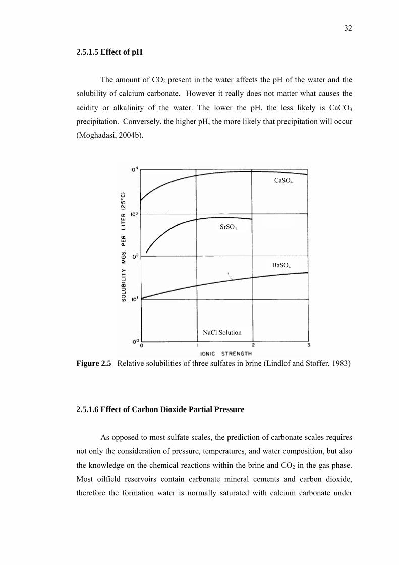
2.5.1.4 Effect of Ionic Strength The solubility of calcium sulfate is strongly affected by the presence and

concentration of other ions in the system. The solubility of calcium sulfate is an

order of magnitude larger than that of strontium sulfate, with in turn is about one and

one- half orders of magnitude larger than that of barium sulfate, as shown in Figure

2.5.

For example, Figure 2.5 indicates that the solubility of strontium sulfate can

be larger than 950 mg/l. This solubility, however, is true only when the solution is

stoichiometrically balanced i.e., when the number of strontium ions equals the

number of sulfate ions. If an excess of either ion is introduced, the solubility is

depressed remarkably. This is known as the common ion effect (Lindlof and Stoffer,

1983). The solubility reaches a maximum in highly concentrated brines.

32

2.5.1.5 Effect of pH The amount of CO2 present in the water affects the pH of the water and the

solubility of calcium carbonate. However it really does not matter what causes the

acidity or alkalinity of the water. The lower the pH, the less likely is CaCO3

precipitation. Conversely, the higher pH, the more likely that precipitation will occur

(Moghadasi, 2004b).

CaSO4

BaSO4

SrSO4

NaCl Solution

Figure 2.5 Relative solubilities of three sulfates in brine (Lindlof and Stoffer, 1983)

2.5.1.6 Effect of Carbon Dioxide Partial Pressure As opposed to most sulfate scales, the prediction of carbonate scales requires

not only the consideration of pressure, temperatures, and water composition, but also

the knowledge on the chemical reactions within the brine and CO2 in the gas phase.

Most oilfield reservoirs contain carbonate mineral cements and carbon dioxide,

therefore the formation water is normally saturated with calcium carbonate under

33

reservoir conditions where the temperature can be as high as 200 °C and the pressure

up to 30 MPa (Moghadasi, 2004b).

Solubility of calcium carbonate is greatly influenced by the carbon dioxide

content of the water. CaCO3 solubility increases with increased CO2 partial pressure.

The effect becomes less pronounced as the temperature increases. The reverse is also

true. It is one of the major causes of CaCO3 scale deposition.

At any point in the system where a pressure drop is taken, the partial pressure

of CO2 in the gas phase decreases, CO2 comes out of solution, and the pH of the

water rises. The amount of CO2 that will dissolve in water is proportional to the

partial pressure of CO2 in the gas over the water (Moghadasi, 2004b).

2.5.2 Zinc Sulfide, Lead Sulfide, and Iron Sulfide Solubilities

Lead and zinc sulfide solubility is much lower even than iron sulfide, which

is the common sulfide in oil field environments. The very low solubility of lead and

zinc sulfide would make it unlikely that zinc/lead and sulfide ions could exist

together in solution for any length of time.

It is more likely that the zinc/lead ion source mixes with the hydrogen

sulfide-rich source within the near wellbore or the production tubing during fluid

extraction; form then on, changes in temperature, solution pH, and residence time

control where scales deposit within the process system.

For example, in a 1M (mole/dm3) NaCl brine solution as presented in Figure

2.6 at pH = 5 the solubility of iron sulfide is 65 ppm, whereas lead and zinc sulfides

are 0.002 ppm and 0.063 ppm respectively. Depending on the exact brine conditions,

the solubility of zinc sulfide is between 30 to 100 times more soluble than lead

sulfide. As with iron sulfide, the solubility of both lead and zinc sulfide increases

with increasing solution pH (Collins and Jordan, 2001).

34

Figure 2.6 Comparison of zinc, lead and iron sulfide solubility in 1M NaCl brine

at 25 °C (Collins and Jordan, 2001)

2.6 Oilfield Scale Types

The most common scales encountered in oilfield operations are sulfates such

as calcium sulfate (anhydrite, gypsum), barium sulfate (barite), and Strontium sulfate

(celestite) and calcium carbonate. Other less common scales have also been reported

such as iron oxides, iron sulfides and iron carbonate. Lead and zinc sulfide scale has

recently become a concern in a number of North Sea oil and gas fields (Collins and

Jordan, 2001). There follows a brief description of each scale.

2.6.1 Calcium Carbonate Scales

Calcium carbonate or calcite scale is frequently encountered in oilfield

operations. But the calcite has the greatest stability in oilfield circumstances, so it is

the most common form of calcium carbonate encountered in oilfield production

operation.

35

Calcium carbonate crystals are large, but when the scale is found together

with impurities in the form of finely divided crystals, then the scale appears uniform.

Deposition of CaCO3 scale results from precipitation of calcium carbonate is as per

the following equation:

Ca+2 + CO3-2 → CaCO3 (2.4)

As it will be seen later calcium carbonate scale can also be formed by

combination of calcium and bicarbonate ions, and this reaction is the major cause of

calcium carbonate scale deposition in oilfield operations. This is because only a

small percentage of the bicarbonate ions dissociated at the pH values found in most

injection waters to form H+ and CO3-2 (Moghadasi et al., 2004b).

In many oilfields, the deposition of calcium carbonate scale on surface and

subsurface production equipment creates an operation problem. The formation water

in which the carbonate-scale-forming components are initially dissolved becomes

supersaturated with calcium carbonate because of the drop in pressure during

production. The continuous flow of a supersaturated solution through the production

equipment results in the growth of a dense layer of calcium-carbonate crystals

(Bezemer and Bauer, 1969).

Carbonate scales frequently appear in the wellbore, especially near the

wellhead where, because of pressure drop, dissolved CO2 escaped from produced

water and caused water pH as well as the saturation index of carbonate minerals to

increase (Zhang and Farquhar, 2001).

In the pre-seawater breakthrough period, calcium carbonate precipitation,

caused by the loss of CO2 from the formation water produced, can be observed.

CaCO3 scaling is not difficult to control by scale inhibitors or by removal with acid.

The water is drained to the surface and suffers from significant pressure drop

and temperature variations during the production. The continuous pressure drops

36

lead to degassing of the carbon dioxide with an increase in pH value of the produced

water and precipitation of calcium carbonate (Mackay, 2003; Rousseau et al., 2003).

Carbonate scale formation occurs when connate water or aquifer water passes

through the bubble point and carbon dioxide is evolved. As carbon dioxide is

evolved, the solubility with respect to carbonate declines rapidly and forms a

precipitate with divalent ions, such as iron, and more commonly calcium, as outlined

in the following equation (Mackay and Jordan, 2005):

3 2 3 2 2Ca (HCO ) CaCO + CO + H O⇔ (2.5)

According to Clemmit et al., (1985), calcium carbonate scale is formed by a

different mechanism. As few waters contain the actual carbonate ion, the scaling

potential arises from decomposition of calcium bicarbonate. This decomposition is

due to the pressure reductions (at chokes or separators) releasing carbon dioxide and

thus moving the equilibrium (with a pH increase) of the above reaction to the right

and producing calcium carbonate. If the quantity of calcium carbonate produced

exceeds its solubility in the water, then precipitation can occur.

2.6.2 Calcium Sulfate Scales

Calcium sulfate scale poses a unique problem for the salts under

consideration because it occurs with one of three different phases. Calcium sulfate

exists in several crystalline forms. These include gypsum (CaSO4.1/2H2O) and

anhydrite (CaSO4).

Gypsum, the most common scale occurs at relatively low temperature. At

higher temperature (above 100 ºC), the stable phase predicted is anhydrite (CaSO4).

However, hemihydrate has been known to form at 100 to 121 ºC, especially in non-

turbulent systems and in high ionic strength brines (Moghadasi et al., 2003a).

37

Calcium sulfate, which is important in desalination geochemistry and

petroleum engineering, is complicated by the fact that it can crystallize from aqueous

solution in three forms: gypsum (CaSO4.2H2O), hemihydrate (CaSO4.1/2H2O) and

anhydrate (CaSO4). These compounds may be stable depending on temperature and

ionic strength and they have decreasing solubilities with increasing temperatures

above 40 ºC. Vetter et al. (1982) have studied the morphology of scale.

Among various types of mineral scales, calcium sulfate is one of major scales

in petroleum industry that can cause sever flow assurance and formation damage

issues. Many parameters are affecting this problem. Temperature, pressure, fluid

concentration, ratio of brine to hydrogen, fluid dynamic and type of porous media are

among these parameters (Tahmasebi et al., 2007).

According to Oddo et al., (1991), calcium sulfate scale formation is

somewhat dependent on temperature, but is typically precipitated because of a

decrease in pressure or an increase in the relative concentrations of calcium or

sulfate. CaSO4 solubility is fairly independent of pH and hence, can readily

precipitate in an acid environment.

The case where water injection (seawater, river, aquifer, or produced water) is

used for pressure maintenance and sweep, the mixing of incompatible brines can lead

to the formation of sulfate scales when the injection water contains sulfate ions

(Mackay and Jordan, 2005).

2+ 2+ 2+ 2

4 4 4-Ba (or Sr or Ca ) + SO BaSO (or SrSO or CaSO ) ⇔ 4 (2.6)

2.6.3 Barium Sulfate Scale

The barium sulfate scaling is a chronicle disaster in waterflood projects with

incompatible injected and formation waters. This is usually due to precipitation of

38

BaSO4 from the mixture of both waters and consequent permeability reduction

resulting in well productivity decrease (Bedrikovetsky et al., 2006).

Barium sulfate scale (barite) in oil fields can be precipitated easily on the

basis of already available information relating to thermodynamic condition and the

kinetics of precipitation (Nancollas and Liu, 1975; Mitchell et al., 1980).

Barium sulfate is the most insoluble scale that can be precipitated from

oilfield waters. It forms a hard scale which is extremely difficult to remove. The

solubility of barium sulfate is about a thousand times less than of calcium sulfate, at

surface conditions.

The solubility of barium sulfate goes up with increasing temperature, pressure

and salt content of the brine. Thus prediction of barium sulfate scale is much easier

than the others since a pressure, temperature or salt content drop will increase

precipitation.

A common case of barium sulfate scale is the mixing of two or more

incompatible waters. Seawater is often used during workovers, or for flooding

formations which contain an appreciable amount of barium ions. Mixing of these

waters represents a risk of subsequent formation and wellbore damage caused by

barium sulfate deposition (Connell, 1983).

In the post seawater-breakthrough period, however, there is a much more

serious problem of precipitation of barium sulfate from an incompatibility between

the formation water and seawater. BaSO4 scale removal is particularly difficult.

Thus, BaSO4 scale treatment must focus mainly on its prevention through the use of

scale-control chemicals. Thus, the severity of the scaling problem is determined both

by the scaling rate and the efficiency of the chemical inhibitors (Mazzollnl et al.,

1992).

39

In most cases, the scaled-up wells are caused by the formation of sulfate

scales of barium and strontium. Due to their relative hardness and low solubility,

there are limited processes available for their removal and the preventive measure

such as the squeeze inhibitor treatment has to be taken. It is therefore important to

have a proper understanding of the kinetics of scale formation and its detrimental

effect on formation damage under both inhibited and uninhibited environment (Wat

et al., 1992).

2.6.4 Strontium Sulfate Scale

Strontium sulfate scale formation has become a growing concern in oil-

production systems (Nassivera and Essel, 1979). Until recently, the appearance of

strontium in oilfield scales has been primarily in the presence of barium sulfate scale.

Almost pure SrSO4 scale now is observed in several production wells around the

world. The scale formation is primarily a result of subsurface commingling of

waters, which results in water supersaturated in SrSO4.

Strontium sulfate solubilities may play a role in many disciplines of science

and engineering. For example, strontium sulfate forms scale in oil and/or geothermal

fields which are frequently accompanied by other sulfates of alkaline earth metals.

Strontium sulfate behaves like barium sulfate except the former is more

soluble under the same conditions. Most of the field scale barium sulfate deposits

contains strontium sulfate too (Essel and Carlberg, 1982; Shen and Corsby, 1983).

2.6.5 Sources of Zinc and Lead and the Mechanism of Sulfide Formation

Zinc sulfide scale is more likely when mixing of incompatible fluids such that of

formation waters rich in zinc with H2S gas in the well caused the deposition of this type of

40

scales. Several sources of zinc/lead and sulfide ions are possible within produced

fluids (Collins and Jordan, 2003).

(1) Potential sources of zinc and lead ions include

(a) Reaction products of formation minerals (sphalerite zinc sulfide (ZnS)

and galena lead sulfide (PbS)) during connate and aquifer water contact

over many millions of years could result in partial mineral dissolution

(Sverjensky, 1984).

(b) Reaction of injected water used for pressure support into the aquifer or

oil leg can result in the fresh or seawater reacting with minerals within

the formation can become enriched in heavy metal ions.

(c) Zinc ions sourced from heavy brine completion fluids lost into the

formation during drilling and well workover operations (zinc bromide).

Biggs (1992) (cited in Collins and Jordan, 2003) reported that a loss of

500 bbls of 17.2 ppg zinc bromide completion fluid within a reservoir

resulted in significant zinc sulfide scale formation with the presence of

2 ppm of hydrogen sulfide from the reservoir.

(d) In an oil field operated in the North Sea UK sector, the presence of zinc

sulfide on downhole gauges and logging tools was reported within a

well where zinc bromide brines had been lost during completion

operations. Zinc levels within the produced fluids were in the region of

10 to 50 ppm for several months during initial water breakthrough.

(2) Potential sources of Sulfide Ions Include

(a) Hydrogen sulfide (H2S) gas is the most likely source of sulfide ions to

allow the formation of lead/zinc sulfide scale. Low concentration (in

the tens of ppm levels) of H2S has been reported in produced gas from

wells where lead and zinc sulfide scale problems have been reported.

41

(b) Decomposition of drilling compounds and corrosion inhibitor can also

produce sulfide ions at high temperature when tested in autoclave

equipment but are very unlikely to be the source of sufficient sulfide

ions to give scale deposition over many years of production. The most

likely source of sulfide ions is from reservoir hydrogen sulfide gas.

2.6.6 Iron Sulfide Scale

Iron sulfide species have been known to cause operational problems in the oil

industry. Iron sulfide scale is present in oil and gas producing wells, sour wells and

water injectors where the injected water has high sulfate content. The sources of iron

are the formation brines (especially in sandstone formations) and the well tubular.

Iron produced by corrosion processes can be minimized by employing various

corrosion protection techniques (Nasr-El-Din and Al-Humaidan, 2001).

According to Raju et al. (2003), the disposal water contains dissolved H2S,

whereas the aquifer water contains dissolved iron. When these two waters are mixed

together, H2S reacts with the iron ions and precipitates iron sulfide species, as shown

in Equation (2.7).

(2.7) ++ +2Fe + H S FeS + 2H⇔ ↓

2.7 Scale Prevention and Removal 2.7.1 Prevention Scale Formation

The most obvious way of preventing a scale from forming during oil

production is to prevent the creation of supersaturation of the brine being handled.

This may sometimes be possible by altering the operating conditions of the reservoir,

for example by ensuring that the wellbore pressure is sufficient to prevent the

42

liberation of gas and by injecting water which is compatible with formation water.

However, economics usually dictate that the use of inhibitors is preferred.

The formation of mineral scale in production facilities is a relatively common

problem in the oil industry. Most scale forms either by pressure and temperature

changes that favor salt precipitation from formation waters, or when incompatible

waters mix during pressure maintenance or waterflood strategies. Scale prevention is

achieved by performing squeeze treatments in which chemical scale inhibitors are

injected in the producers near wellbore (Romero et al., 2007).

2.7.1.1 Operational Prevention There are two operational preventions:

(1) Avoid mixing Incompatible Waters

The importance of avoiding incompatibility problems should be obvious from

the preceding discussion. However, in offshore locations like the North Sea

there is no economic method of obtaining compatible water, so sea water

must be used.

(2) PH Control

Lowering the pH will increase the solubility of carbonate scales (but may

cause corrosion problems). This method is not widely used in the oilfield,

since accurate pH control is needed. However, it is useful for cooling waters.

2.7.2 Scale Control Chemicals

In oil and gas well operations, water-insoluble scale is formed in tubing,

casings, and associated equipment, as well as in the wellbore and the formation itself,

43

which carry, at least in part, water or brine waters. These waters can contain

insoluble calcium, barium, strontium, magnesium, and iron salts.

Scale inhibitors are chemicals which delay, reduce or prevent scale formation

when added in small amounts to normally scaling water. Most of modern scale

inhibitors used in the oilfield functions by one or both of the following mechanisms

(Connell, 1983):

(1) When scale first begins to form, very tiny crystals precipitate from the water.

At this point, the scale inhibitor absorbs onto the crystal surface thus

preventing further growth.

(2) In some cases, scale inhibitors prevent the scale crystals from adhering to

solid surfaces such as piping or vessels.

According to Bezemer and Bauer (1969), the most common classes of

inhibitor chemicals are inorganic phosphates, organophosphorous compounds and

organic polymers. Polyphosphonocarboxylic acid (PPCA) and

Diethylenetriaminepenta (methylenephosphonic acid) (DETPMP) are two common

commercial scale inhibitors used in the oil and gas industry. Normally, PPCA is

regarded as nucleation inhibitor and DETPMP as a growth inhibitor (Chen et al.,

2004).

In the majority of cases, a good scale inhibitor should be effective at 5-15

ppm in clean water. However, if substantial amount of suspended solids are present,

higher inhibitor concentrations will be necessary. Moreover, the reason being that

the inhibitor will adsorb onto surface of the solids in the water, thereby reducing the

amount available to inhibit scale formation.

Scale inhibitors that are periodically pumped down production wells and into

the producing formation for short distances around the wellbore have been developed

and are widely utilized. The inhibitor contacts the formation and is adsorbed onto

the reservoir petrofabric. It is later slowly released into the produced fluids, thereby

44

inhibiting the formation of sulfate scales for some period of time, usually several

months. When the inhibitor concentration levels fall too low to be effective, the well

is again squeezed with chemical and the cycle is repeated. This technique is widely

known as squeeze inhibition (McElhiney et al., 2001).

The formation of mineral scale (carbonate/sulfate/sulfide) within the near

wellbore, production tubing and topside process equipment has presented a challenge

to the oil and gas industry for more than 50 years. Chemical methods to control scale

have been developed including scale squeeze treatments and continual chemical

injection. A key factor in the success of such treatments is the understanding of

chemical placement and the effectiveness of the treatments chemicals (Jordan et al.,

2006b).

Squeezing is the most common method for scale control downhole. Scale

inhibitor, diluted in brine, is displaced into the producing formation where it is

retained and then released slowly back into the aqueous phase during normal well

production. Squeeze inhibition is effective in a wide variety of situations; however,

it has some drawbacks. The squeeze chemical, often a phosphonate or high

molecular weight sulphonate, is usually dissolved and diluted in water for transport

down the wellbore.

Several challenges must be overcome in order to develop an effective

combined scale removal and scale inhibition treatment. The most notable are (Smith

et al., 2000):

(1) Cost

The combined treatment has to offer an economic advantage when compared

to serial stimulation and inhibition treatments.

(2) Corrosion control

The scale inhibitor must not cause a significant change in the corrosivity of

the stimulation system. If the stimulation system requires the use of a

corrosion inhibitor then the scale inhibitor must not prevent its function.

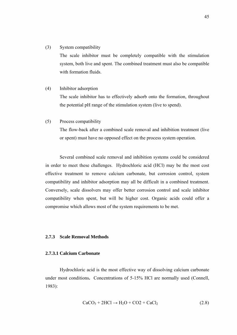
45

(3) System compatibility

The scale inhibitor must be completely compatible with the stimulation

system, both live and spent. The combined treatment must also be compatible

with formation fluids.

(4) Inhibitor adsorption

The scale inhibitor has to effectively adsorb onto the formation, throughout

the potential pH range of the stimulation system (live to spend).

(5) Process compatibility

The flow-back after a combined scale removal and inhibition treatment (live

or spent) must have no opposed effect on the process system operation.

Several combined scale removal and inhibition systems could be considered

in order to meet these challenges. Hydrochloric acid (HCl) may be the most cost

effective treatment to remove calcium carbonate, but corrosion control, system

compatibility and inhibitor adsorption may all be difficult in a combined treatment.

Conversely, scale dissolvers may offer better corrosion control and scale inhibitor

compatibility when spent, but will be higher cost. Organic acids could offer a

compromise which allows most of the system requirements to be met.

2.7.3 Scale Removal Methods 2.7.3.1 Calcium Carbonate

Hydrochloric acid is the most effective way of dissolving calcium carbonate

under most conditions. Concentrations of 5-15% HCl are normally used (Connell,

1983):

CaCO3 + 2HCl → H2O + CO2 + CaCl2 (2.8)

46

A corrosion inhibitor must be added to the acid to stop it from attacking the

pipework and a surfactant is usually added to make the surfaces water wet.

2.7.3.2 Calcium Sulfate The following may be used to dissolve calcium sulfate (Connell, 1983):

(1) Converters Inorganic converters are usually carbonates or hydroxides which react with

calcium sulfate and convert it to acid soluble calcium carbonate or calcium

hydroxide. The conversion treatment is then followed by a hydrochloric acid

treatment to dissolve the resulting scale:

CaSO4 + (NH4)2CO3 → (NH4)2SO4 + CaCO3 (2.9)

Then CaCO3 + 2HCl → H2O + CO2 + CaCl2 (2.10) (2) Solvents:

Solvents are now available which will completely dissolve gypsum scale.

Other compounds used (to s lesser extent) are EDTA and salt water.

2.7.3.3 Barium Sulfate One of the most common reasons for production loss is the development of

scales inside the production strings, blocking the flow of the reservoir fluid to the

surface facilities. Barium sulfate scale is among the toughest scales to remove,

whether mechanically or chemically (Guimarases et al., 2007).

47

Barium sulfate could only be removed by mechanical means. However,

chemicals based on EDTA are now available which have had some success in

dissolving barium sulfate.

2.8 Scale Prediction 2.8.1 Laboratory Evaluation

Scale formation can be predicted by laboratory experiments. Several

experimental studies have been conducted to determine the scaling potential in

different oilfields. The detailed experimental parameters are listed in tables in

Appendix A.

Mitchell et al. (1980) conducted to investigate experimentally the effect of

incompatibility of injected water and formation water in the Forties field. They used

a core with six injectors at one end and one outlet at the other end to simulate a

production well. The flow rates of injection and formation water were adjusted so

that one part of injection water was injected to ten parts of formation water.

They found that the injection pressure remained relatively constant most of

the time and then increased rapidly just before the core became completely

blocked. They stated that the initial scale deposition occurred around the surfaces of

the pores. As more scale was deposited, the pore-throat flow area was reduced.

Read and Ringen (1982) investigated a series of laboratory tests to evaluate

the extent of formation damage which could result from scales formed within the

porous rock in North Sea oil reservoir. These tests were performed in glassware,

bead packs, and synthetic alumina cores. Initially, the formation water and seawater

were analyzed. It showed that mixtures of these waters could precipitate both

strontium and barium sulfate.

48

From analyses, the weight of precipitates of these salts was calculated based

on solubility products. To confirm these calculations, blends of both waters were

mixed in glassware and the total amount of precipitate was determined by filtering

and weighing. As a check, the precipitate was also re-dissolved in dilute HC1 and

the concentrations of calcium, strontium, and barium were determined by atomic

absorption analysis.

Nevertheless, for mixing test in porous media, were also conducted in a pack

of 4 mm glass beads and in synthetic alumina cores that were 4 inches in length and

3/2 inches in diameter. The mixing test was all conducted at reservoir temperature

70°C, no pressure was applied during a test. The cores were first saturated with

formation water, and a base permeability determined. Core flooding was done in

varying proportions of seawater and formation water and pressure differential was

continuously recorded throughout the flow.

From the experimental results, it was the worst permeability loss occurred

with highest amount of precipitation for lower proportion of seawater. The core test

in which 10% seawater was used shows a dramatic increase in the differential

pressure, as rapid blocking was observed due to scale deposition.

Lindlof and Stoffer (1983) conducted a laboratory study to evaluate possible

strontium sulfate and calcium sulfate scaling associated with the injection of seawater

into the Arab-D reservoir in Saudi Arabia. The laboratory tests showed no

measurable reduction in permeability due to incompatibility effects between Arab-

D formation water and seawater when the two waters mix in the pore channels

during displacement of one water by the other. They described that mixing of Arab-

D water with seawater in various proportions demonstrated that strontium sulfate

could be precipitated.

Todd and Yuan (1990) presented the results of laboratory experiments carried out

at room temperature to investigate the formation of barium sulfate and strontium sulfate

[(Ba, Sr)SO4] solid solution in multi-pressure-tapped cores. Two brines, one barium-and

49

strontium-rich and the other sulfate-rich, separately to the front face of a core plug to

ensure that the two brines mixed uniformly immediately after entering the core. Pressure

differentials were measured and the changing permeability distribution along the core

length was calculated. The morphology and chemical analysis of scaling crystals as

shown by Scanning Electron Microscopy (SEM) are presented.

Results show a large extent of permeability damage caused by [(Ba, Sr) SO4]

solid solution deposits on rock pore surface. The rock permeability decline and

morphology and size of the scaling crystals indicate the influence of the supersaturations

of BaSO4 and SrSO4 and the concentration ratio of barium to strontium ions.

Bezerra et al. (1990) conducted a laboratory study to investigate the

deposition of barium and strontium sulfate scales in producing wells of the

Namorado field. Two incompatible waters one barium-and strontium-rich formation

water and the other sulfate-rich sea water injected into sandstone cores to study scale

formation in porous media. Pressure data were used to calculate the permeability of

the sandstone as a function of the injected fluids. A significant drop in permeability

around 65% was observed after precipitation.

Todd and Yuan (1992) described a laboratory study carried out at 70ºC to

examine (Ba, Sr) SO4 solid-solution scale formation in porous media under the

influence of flow and in static bulk solutions. Two incompatible waters were injected

into a core to study scale formation in porous media, and static scale precipitation

tests were performed in glass jars. Synthetic North Sea water and two formations

waters were used in elevated temperature experiments to simulate field scale

formation. Firstly, the formation water (water M) had medium scale precipitation

when mixed with seawater and the other (water ST) had severe scaling tendency.

Results of experiments carried out at the elevated temperatures again

demonstrate that substantial scale deposition could occur in a rock core and could

cause considerable decline of rock permeability resulting from the mixing of two

incompatible waters.

50

Allaga et al. (1992) described two linear flooding experiments of permeability

reduction of sandpacks caused by solids generation and migration. Type A

experiments investigated the effects that precipitates had on the permeability

reduction of unconsolidated sandpacks. The initial permeabilities of the sandpacks

were adjusted with a mixture of silica flour and sand. In type B experiments, they

measured the ion and solid waves produced while the precipitation/dissolution

reactions were occurring in the sandpacks. Two solids, calcium and barium sulfate

crystals, were injected into and generated within the sandpacks by chemical reaction.

Furthermore, a precipitate formed when two solutions, one solution rich in

sulfate ions and another solution rich in barium or calcium ions, were mixed inside

the sandpack. Calcium and barium sulfate precipitates did not plug the sandpacks to

the same extent. One experiment with barium sulfate precipitate produced a 60%

reduction in initial permeability. Calcium sulfate precipitates consistently plugged

all sandpacks, causing a 10% to 20% reduction in the original permeability.

Wat et al. (1992) presented results of BaSO4 formation kinetics in both

beaker tests and in highly reproducible sandpacks which simulates the flow in porous

medium. Synthetic North Seawater and formation water were mixed inside the

sandpack to study scale formation in porous media. For the in-situ scaling

experiments, the crystal growth process appeared to be localized. The permeability

decline was likely caused by the continuous growth of crystals and not by particle

transport and flow blockage. The scale precipitation process in porous medium was

likely to be dominated by heterogeneous nucleation with the [Ba++] ion concentration

in the sandpack effluents consistently less than that of similar beaker tests.

Nevertheless, the scale morphology varies considerably from the point of

mixing. Under steady state, the scaling process within the porous medium was

contributed by a range of supersaturated mixtures. The point where the incompatible

brines first come into contact with each other has the highest supersaturation and

with maximum amount of deposit. Furthermore, results of in-situ scaling in highly

51

reproducible sandpacks have been included to provide information on likely

formation damage and comparison of crystal growth under static and dynamic flow

environment.

Jordan et al. (2000) conducted an experimental work to develop an effective

treatment strategy for production wells in North Slope Alaska, specifically those with

electrical submersible pumps (ESP’s) that suffered significant performance

impairment at water cuts of less than 5% because carbonate scale deposited within

the ESP’s. During the injection at different stages, the formation water is rich in

cations (Ba, Sr, and Ca) and the injection water is rich in anions (SO4) into porous

medium.

Furthermore, at very low water cut (<1%), scale formation could cause

operational problems with downhole production equipment. It was possible to form

not only conventional calcium carbonate scale from produced water, with high

bicarbonate and high calcium levels, but also iron carbonate deposited from a

combination of iron from formation water and corrosion products.

McElhiney et al. (2001) conducted a laboratory study to investigate the

problem of in-situ barium sulfate precipitation in West Africa offshore reservoir.

Core flooding experiments conducted at frontal velocities of 0.31 m/day in fired

Berea sandstone cores to evaluate in-situ barium sulfate precipitation at ambient

temperature (~ 70°F) and atmospheric pressure. Synthetic raw seawaters

containing low and high sulfate contents were mixed in-situ with formation water

containing dissolved barium ions before injection.

Furthermore, the precipitation loss of barium sulfate was observed by the

measurement of the effluent profiles of sulfate ion and barium ion. The results

indicated that for low sulfate seawater, the barium sulfate scaling potential was

reduced, which was also verified by SEM analysis.

52

Moghadasi et al. (2002) presented an experimental and theoretical study of

calcium sulfate scale formation and particle movement in the porous media used of

packing bed with twelve different sizes of the glass and sand bead and the eight core

plug that gathered from the Siri oilfields. Two incompatible waters, Persian Gulf

water and Mishrif formation water were injected into a core to study scale formation

in porous media.

Moreover, permeability decrease was affected by the following parameters:

solid particle concentration, flow rate, and the initial permeability of porous medium.

The high rates of permeability damage happened under conditions of high

concentration of solid particles, small ratio of solid particle size to the mean diameter

as well as low flow rates in low permeability porous media during water injection.

One of the important factors in permeability reduction because of the movement of

internal solid particles was the sticking factor.

Furthermore, the modeling results provided same information for

understanding the mechanisms of permeability alteration resulting from solid particle

invasion into a porous medium.

Collins and Jordan (2003) conducted an experimental study to investigate the

deposition of zinc sulfide scale that had been found in several fields along the Gulf

Coast of the U.S.A. and in fields within the North Sea Basin at high temperature and

high salinity. Lead and zinc sulfide scales were very insoluble at typical formation

brine pH and salinity. Their solubility increased with increasing brine salinity,

temperature and falling pH.

Nevertheless, lead and zinc sulfide scale occurrence have been reported when

high salinity brines were produced along with oil and gas within the Gulf of Mexico,

onshore U.S.A. and North Sea (both UK and Norwegian sector). The formation of

such deposits could result in expensive mitigation and significant differed oil

production.

53

Moghadasi et al. (2003b) presented an experimental and theoretical study of

permeability reduction of porous media caused by scaling. Each solution system

consisted of two salts, one rich in calcium ions and the other rich in sulfate or

carbonate ions, which were kept separate until they had entered the porous medium.

Since mixing calcium nitrate and sodium sulfate or sodium carbonate results in

calcium sulfate or calcium carbonate which crystallizes on the porous medium.

Permeability decline caused by scale formation in the porous medium ranged

from less than 30% to more than 90% of the initial permeability, depending on

solution composition, initial permeability, temperature, flow rate, and solution

injection period. The pattern of permeability decline in a porous medium due to

continues scaling was characterized by a concave curve with a steep initial decline,

which gradually decreased to a low.

Nevertheless, the initial steepness of those curves generally decreased with

increasing distance from the point of mixing of incompatible solutions. Several

factors influencing scale formation had been examined. Increasing temperature,

supersaturation and flow rate had a detrimental effect on the permeability reduction.

Flow rate caused more for calcium carbonate precipitation than calcium sulfate.

Voloshin et al. (2003) studied core flooding tests for western Siberian oil

fields. They concluded that injected water salinity and the mineralogical composition

of formation rock played an important role in the process of scaling in the reservoirs

and the wells. During interaction with the rock, the injected water changed its ionic

composition, becoming richer in either carbonates or sulfates, or both.

Furthermore, analysis of electric submersible pump deposits showed that

carbonates (calcium and magnesium), quartz, chlorite, and gypsum were present in

the mineral composition of the scale deposits. While carbonates were among the

main components of the deposits, chloride and gypsum were present in negligible

quantities in every sample. In some deposits, siderite and iron oxide were present

too.

54

Nasr-El-Din et al. (2004) described a laboratory study to utilize high sulfate

pit brine and calcium chloride solutions as a means to permeability of water

producing zones. Two incompatible waters one contains high concentration calcium

ions and other contains high sulfate content were injected into carbonate core from a

carbonate reservoir in Saudi Arabia. Compatibility tests indicated immediate

precipitation of calcium sulfate when pit water and calcium chloride brines were

mixed.

Nevertheless, coreflood testes indicated that maximum core plugging

occurred when pit brines were injected into cores saturated with CaCl2 brines. The

degree of core damage depended on the injection rate.

Moghadasi et al. (2004a) presented an experimental and theoretical study of

permeability reduction of porous media caused by scaling. Two incompatible

solutions of calcium and sulfate/carbonate ions were injected into the porous

medium, where calcium sulfate or calcium carbonate was generated by chemical

reaction.

They concluded permeability decline caused by scale formation in the porous

bed ranged from less than 30% to more than 90% of the initial permeability,

depending on solution composition, initial permeability, temperature, flow rate, and

solution injection period. The pattern of permeability decline in a porous medium

due to scaling injection was characterized by a steep initial decline which gradually

slowed down to a lower. Several factors influencing scale formation had been

examined. Both increasing temperature and flow rate had a detrimental effect on the

permeability reduction.

Strachan et al. (2004) performed laboratory studies to estimate the suitability

of aqueous and non-aqueous scale inhibitors for downhole application in dry and

lower water cut wells in the Magnus field. Synthetic brine Magnus formation water

and seawater were injected into the porous medium. Corefloods connected to a novel

water block remover indicated no formation damage was observed with the polymeric

55

and phosphonate precipitation inhibitors and those treatment packages were

considered to be suitable for pre-emptive squeeze in the BP Magnus field.

Ahmed (2004) presented an experimental and theoretical study of

permeability reduction of porous media caused by scaling. Two incompatible

solutions containing Ca+2 and SO4-2 ions injected into Berea sandstone cores, which

were kept separate until entering the porous medium.

The results indicated increased rate of CaSO4 precipitation at higher

temperatures, higher flood velocities, and greater brine supersaturation, whereas

pressure had a slight effect on CaSO4 precipitation. Moreover, the results were

utilized to build a general reaction rate equation to predict CaSO4 precipitation in

Berea sandstone for a given temperature, brine supersaturation, and flooding

velocity.

Bedrikovetsky et al. (2005) conducted a laboratory study to determine

chemical reaction rate constant versus flow velocity in porous media for scaling

conditions in field N (Brazil). Two incompatible waters, one barium-rich formation

water and the other sulfate-rich sea water injected into outcrop RB (Brazil) cores.

Two series of steady state testes on simultaneous injection of formation and injection

waters with barium sulfate formation have been performed for different velocities in

two cores. It was shown that the chemical reaction rate constant is proportional to

flow velocity, in the range studied.

2.8.2 Modeling Development

Today scale prevention is the way oilfield operators choose, when touched

with scaling problems in oilfield production, as scale prevention is technically and

economically more effective than redissolution, once scale has formed. One

essential step in scale prevention is scale prediction. Along with laboratory

56

experiments, scale formation can be predicted by several models to determine the

scaling potential in different oilfields.

Vetter et al. (1982) presented a model for predicting simultaneous

precipitation of barium sulfate, strontium sulfate and calcium sulfate. Water

compositions, pressure and temperature were taken into account. They showed the

effect of scaling of a less soluble sulfate, such as BaSO4, on the precipitation of more

soluble salts such as SrSO4 and CaSO4. The scale component has the lowest solubility

product (e.g. BaSO4) that precipitates first because of removal of some sulfate ions

from the solution.

Furthermore, the new ionic product required for calculating this precipitation is

adjusted for BaSO4 precipitation. This is followed by the precipitation of the second

component having the larger solubility product (e.g. SrSO4). Finally the last

component of this series, CaSO4, will precipitate. The entire process is repeated

and continuous re-dissolution and precipitation of all scale-forming compounds

(BaSO4, SrSO4 and CaSO4) for each set of thermodynamic conditions at which

precipitation can occur.

Bertero et al. (1988) presented a numerical model which couples a reservoir-

fluid-flow/thermal-equilibrium simulator with a chemical-equilibrium computer

code. The reservoir simulator, called AGIPS, is a finite-difference numerical model

which calculates the evolution in time of the amount of scale formed in any point of

the reservoir and inside the wells when changes occur in the temperature of the

injected water and when the injection water mixes with reservoir brine.

Nevertheless, the model calculates temperature and pressure profiles in the

reservoir, together with their evolution in time, taking into account the permeability

reduction caused by scale formation. For validation of their model, mixtures with

different proportions of injection and reservoir water (taken from North African oil

fields) were prepared and kept in a pressure vessel at reservoir conditions.

57

The Results were presented for the chemical-equilibrium code validation by

matching experimental data on scale formation in mixtures of incompatible waters.

An example is also given of AGIPS use in simulating a five-spot waterflood where

incompatible water is injected.

Yuan and Todd (1991) developed a model for predicting sulfate scaling

problems due to commingling of chemically incompatible waters as well as by

temperature and pressure changes. This model is based on the Pitzer equation

and has proved to be successful in calculating sulfate solubilities over wide ranges

of solution compositions and temperature. The model is capable of predicting the

scaling tendencies of barium, strontium and calcium sulfates at various water

compositions, temperature, and pressures covering oil field conditions.

The model also predicts competitive simultaneous co-precipitation of BaSO4,

SrSO4, and CaSO4, where sulfate is a common ion, reflecting the precipitation of

more than one sulfate mineral. Moreover, this model was used in evaluating the

sulfate scaling potentials resulting from mixing North Sea injection water with

Forties formation water. The predicted scaling precipitation was substantiated by

field observations.

Yeboah et al. (1993) developed Oilfield Scale Prediction Model (OSPMod)

which predicts the potential and deposition profile based on extensive

thermodynamic and kinetic data. The first major step of the model is to use the

input data (produced water analysis and thermo-chemical data) to determine the

thermodynamic scaling potential. If scale is predicted to form, the next step is to use

kinetic and well data to determine the scale deposition profile from bottomhole to the

surface. Thus, it computes the deposition profile as a function of position and time if

a well is predicted to scale.

In addition to the highly informative and attractive graphic display of results,

the model provides extensive tabulation of the results including calculation of

densities, activity coefficients, solubilities, supersaturations, solubility product

58

constants, equilibrium composition (including pH, partial pressure of CO2 and

HCO3 ) saturation indices, concentration, velocity, amount and type of scale and

available cross-sectional area at different positions and times.

Thomas et al. (1995) developed an expert system for prediction and analysis of

the damage potential in the oilfield during production and injection due to

interactions between the fluids and the solid phase. These interactions are because

of hydro-mechanical processes and/or changes in physiochemical conditions of the

fluid (pH, temperature, ionic strength) and cause a reduction in the permeability of

the reservoir rocks and technical equipment. The expert system FROCKI (Fluid-

Rock-Interactions) was written in LISP as an object-oriented computer language to

manage all these problems of oil fields.

Moghadasi et al. (2003a) developed a model which was based on

experimental data and empirical correlations that perfectly matched Iranian oilfield

conditions where water injection was performed for reservoir pressure maintenance.

The first step of the model is to use the water analysis and physical conditions

(temperature and pressure) to determine the scaling potential. If scale is expected to

form, the next step is to use kinetic and well data to compute the scale deposition.

Furthermore, this model can be applied to predict scaling deposition because

of commingling of chemically incompatible waters within the system. The model

predicted the effect of temperature, pressure, and pH on scale formation. It was

found that CaCO3 scale formation increased with increase in temperature, a decrease

in pressure and an increase in pH. The precision of the results was found to be

affected only by the occurrence of water sampling and water analyzing.

Rousseau et al. (2003) applied a model to find quick correlations between

physical measurements and the predicted risk of scaling in Angolan reservoirs which

are dolomitic with temperatures ranging from 150 to 164 °C with a nearly constant

pressure (320 bar). The model took into account the cumulated effects of water flow

in connection with pressure and temperature variations, and changes in dynamic

59

water composition because of the mixing. Here, the kinetic module of the

SCALE2000 software was used to explain the scaling phenomenon.

Mackay (2003) developed a model for scale deposition, which was an

extension of his work on mixing of injected, connate, and aquifer brines in water

flooding and its relevance to oilfield scaling. In this model, the location of maximum

scale deposition and the resulting brine compositions at the production wells are

calculated for a range of sensitivities, including reservoir geometry (1D, 2D aerial

and vertical, and 3D), well geometry and the reaction rate.

Moreover, limitations to his modeling work were lack of kinetic reaction rates,

mixing zone, and impact on permeability. Mixing of brines in the wellbore was not

discussed as well, although there was obviously a relationship between in-situ

deposition and the availability of scaling ions that may damage the tubing.

60

2.9 Summary From the survey of the literature, most of the flooding experiments contain

normal salinity (normal concentration of calcium and strontium) and normal

concentration of barium and they were conducted with different media like bead

packs, sandpacks, and alumina cores, and were run at either low or particular

temperatures and pressures.

This research was conducted as an experimental study, containing high

salinity (high concentration of calcium and strontium) and high concentration of

barium, to investigate permeability reduction by deposition of scale formation in

sandstone cores.

CHAPTER 3

METHODOLOGY

3.1 Introduction

This chapter outlines the experimental research work to be done in order to

achieve the objectives of this study. Materials used, design of the experimental

equipment, set up and experimental procedure are all described in the following

sections.

3.2 Materials Used

The materials used in this study were:

3.2.1 Porous Medium

In all flooding experiments, sandstone cores from Malaysia with 3 inch

length and of diameter 1 inch with average porosity of 32% and of initial

permeability varied from 12.30 to 13.87 md were used. No oil was present in the

cores. All the cores were cleaned using methanol in Soxhlet extractor and dried in a

Memmert Universal Oven at 100 °C for overnight before use. Table 3.1 lists the

physical properties of all core samples used in this study.

62

Table 3.1: Physical properties of sandstone cores used in this study

Core of run #

Length

(inch)

Diameter

(inch)

Pore volume

(cm)

Porosity

(%)

Absolute permeability

(md) 1 3 1 4.46 29.81 12.76 2 3 1 5.20 34.75 13.46 3 3 1 4.39 29.34 13.52 4 3 1 5.67 37.89 12.40 5 3 1 5.57 37.23 13.34 6 3 1 4.69 31.35 12.30 7 3 1 5.47 36.56 12.85 8 3 1 5.10 34.09 12.70 9 3 1 4.95 33.08 12.36 10 3 1 5.79 38.70 13.84 11 3 1 5.46 36.49 13.60 12 3 1 4.56 30.48 13.70 13 3 1 4.37 29.21 12.53 14 3 1 5.36 35.82 13.55 15 3 1 5.64 37.69 12.41 16 3 1 4.80 32.08 12.96 17 3 1 5.51 36.83 12.83 18 3 1 4.96 33.15 12.45 19 3 1 5.49 36.69 12.98 20 3 1 6.22 41.57 12.85 21 3 1 5.39 36.02 12.47 22 3 1 4.65 31.08 12.55 23 3 1 5.40 36.09 13.57 24 3 1 4.75 31.75 12.43 25 3 1 4.51 30.14 13.87 26 3 1 4.72 31.55 13.63 27 3 1 4.43 29.61 13.73 28 3 1 6.91 46.18 12.87 29 3 1 6.13 40.97 12.72 30 3 1 4.12 27.54 12.38 31 3 1 4.38 29.27 12.42 32 3 1 5.53 36.96 13.36 33 3 1 4.58 30.61 12.32 34 3 1 4.98 33.28 12.78 35 3 1 5.37 35.89 13.48 36 3 1 4.02 26.87 13.54

63

3.2.2 Brines

The ionic compositions of synthetic formation water and water injection

(Barton and Angsi seawaters) are given in Tables 3.2 and 3.3. Note that the

formation water contained calcium, strontium, and barium ions, and the seawater

contained sulfate ions. It was clear that the mixing of these waters could lead to

calcium, strontium, and barium sulfate precipitation.

Seven salts used for the preparation of synthetic formation water and water

injections were given in table 3.3. The description of these salts is as follow:

(1) Sodium Chloride grade (AR) NaCl (M.Wt. = 58.44 g/mol, 99.8% purity)

supplied by QReCTM.

(2) Potassium Sulfate K2SO4 (M.Wt. = 174.25 g/mol, 99% purity) supplied by

BHD chemicals Ltd Pool England.

(3) Magnesium Chloride MgCl2.6H2O (M.Wt. = 203.30 g/mol, 98% purity)

supplied by R&M Chemicals.

(4) Calcium Chloride (dihydrate) grade (AR) CaCl2.2H2O (M.Wt. = 147.02

g/mol, 78% purity) supplied by QReCTM.

(5) Sodium Bicarbonate NaHCO3 (M.Wt. = 84.01 g/mol, 99.5% purity) supplied

by GCE Laboratory Chemicals.

(6) Strontium Chloride (6-hydrate) SrCl2.6H2O (M.Wt. = 266.62 g/mol, 99%

purity) supplied by GCE Laboratory Chemicals.

(7) Barium Chloride (dihydrate) grade (AR) BaCl2.2H2O (M.Wt. = 244.28 g/mol,

99% purity) supplied by QReCTM.

64

Table 3.2: The ionic compositions of synthetic formation and injection waters

Ionic Normal salinity

formation water (ppm)

High salinity


Normal barium


High barium


Barton seawater

(ppm)

Angsi seawater

(ppm) Sodium 52,132 52,132 42,707 42,707 9,749 10,804.50

potassium 1,967 1,967 1,972 1,972 340 375.05 Magnesium 4,260 4,260 102 102 1,060 1,295.25

Calcium 7,000 30,000 780 780 384 429.20 Strontium 500 1,100 370 370 5.4 6.577

Barium 10 10 250 2,200 <0.2 - Chloride 99,653 146,385 66,706 67,713 17,218 19,307.45Sulfate 108 108 5 5 2,960 2,750

Bicarbonate 350 350 2,140 2,140 136 158.80

Table 3.3: Compounds of synthetic formation and injection waters

Compound Normal salinity

formation water

(ppm)

High salinity

formation water

(ppm)

Normal barium

formation water

(ppm)

High barium

formation water

(ppm)

Average between Barton

and Angsi seawaters

(ppm) Sodium Chloride

132,000 132,000 106,500 106,500 26,100

Potassium Sulfate

- - - - 5,180

Magnesium Chloride

35,625 35,625 853 853 9,846

Calcium Chloride

25,677 110,045 - - -

Sodium Bicarbonate

482 482 - - -

Strontium Chloride

1,521 3,347 - - -

Barium Chloride

- - 445 3,914 -

3.3 Equipment Set-up

A schematic diagram and photograph of the experimental set-up used in this

study were shown in Figures 3.1 and 3.2 respectively. It comprised:

65

Figure 3.1 Schematic of th

Figure 3.2 Photograph of t

3.3.1 Core Holder

A Hassler type, stainless steel core

samples, 3 inch length and 1 inch diameter, w

by TEMCO, Inc., USA and could withstand

of core holder is shown in Figure 3.3.

Oven

Tra

S.W

Water bath Pump

Water tank

valv

Digital readout
Pressure transducer
e coreflooding apparatus

he coreflooding apparatus

holder designed for consolidated core

as used. The holder was manufactured

pressures upto 10,000 psia. Photograph

Core holder

nsfer cell

To nitrogen cylinder

e

Brine collection

66

The core sample is housed inside rubber sleeve. An end plug made of

stainless steel is inserted into end of the sleeve and is pressed against the core sample

by a retaining screw. End plug have circular grooves to ensure fluid injection into

and production from the entire cross-section of the core. The outlet plug has one

production port at the center.

The annular space between the sleeve and the core holder body is filled with

a confining fluid and is pressurized up to the desired pressure. This pressure

prevents fluid by-pass around the core and ensures good sealing between the ferrules

and sleeve. The confining pressure was applied using cylinder of nitrogen gas.

Figure 3.3 Core holder

3.3.2 Fluid Injection Pump

Double-piston plunger pump (Figure 3.4) manufactured by Lushyong

Machiney Industry Limited, with 1.5 horse power motor, maximum design pressure

of 35 bars and approximate flow rate of 20 L/min was used to inject the brines during

flooding at different pressures.

67

Figure 3.4 Double- piston plunger pump 3.3.3 Transfer Cell

Stainless steel transfer cell (Figure 3.5) manufactured by TEMCO, Inc., USA

which can withstand pressures up to 10,000 psia was used to store and pump the

injected brine to the core holder. The cell with a capacity of 1000 ml has a free-

floating piston, which separates the pump fluid (distilled water) from the injection

brine. The pump fluid was pumped into a transfer cell to displace the brine into the

core.

Figure 3.5 Stainless steel transfer cell

68

3.3.4 Oven

During all flooding runs, the core holder was placed inside a temperature

controlled oven is shown in Figure 3.6.

Figure 3.6 A temperature controlled oven 3.3.5 Pressure Transducer

The differential pressure across the core during flooding runs was measured

by using a pressure transducer (model E-913 033-B29) manufactured by Lushyong

Machiney Industry Limited, with a digital display, as shown in Figure 3.7.

Figure 3.7 Pressure transducer with a digital display

69

3.3.6 Laboratory Thermal Equipment (Water Bath)

During all flooding runs, the transfer cell was placed inside a temperature

controlled bath, as shown in Figure 3.8 and manufactured by TEMCO, Inc., USA.

Figure 3.8 A temperature controlled water bath 3.3.7 Vacuum Pump

Two stage high vacuum pump (Figure 3.9) manufactured by TEMCO, Inc.,

USA was used for air evacuation during core saturation.

Figure 3.9 Vacuum pump

70

3.3.8 A Core Cutter Purchased

A core cutter purchased from Norton, USA, was used to cut the sandstone

cores, as shown in Figure 3.10.

Figure 3.10 Sandstones cutting equipment 3.3.9 Soxhlet Extractor

Before each run, the core sample was cleaned for five hours by methanol in

Soxhlet extractor, as shown in Figure 3.11. It consists of round bottle, sample

holder, and condenser.

Figure 3.11 Soxhlet extractor

71

3.3.10 Memmert Universal Oven

Before each run, the core sample was dried for overnight in a temperature

controlled oven at 100°C as shown in Figure 3.12.

Figure 3.12 Memmert universal oven 3.3.11 Viscometer

Brookfield viscometer (model PV III head unit, USA) equipped with a

circulated temperature water bath was used for measuring injection brines viscosities

at various temperatures is shown in Figure 3.13.

Figure 3.13 Brookfield viscometer with a circulated temperature water bath

72

3.3.12 Auxiliary Equipment and Tools

Many other pieces of equipment and tools were used during this study. These

include pressure gauges, thermocouples, stainless steel fittings and tubings, valves,

filters, water tanks, nitrogen cylinder, weighing balance, conical and round bottom

flasks of different capacities, and plastic bottles for sampling.

3.4 Experimental Procedure

The general purpose of the laboratory study was to investigate permeability

reduction by deposition of scale formation in a porous medium and knowledge of

solubility of scale formation and how its solubilities were affected by changes in

salinity and temperature.

3.4.1 Beaker Test

The intent of this study was to determine solubility of common oil field scales

from mixing synthetic brines (formation water and sea water) at high salinity (high

concentration of calcium and strontium), high concentration of barium, various

temperatures (40 to 90 °C) and 1 atm.

The experimental procedures used in the determination of solubility of

common oil field scales from mixing synthetic brines (formation water and sea water)

were:

(1) For each experiment of common oil field scales, 100 mL of each filtered

opposite waters were poured simultaneously into a beaker.

73

(2) The synthetic brines were heated on hot plate, as shown in Figure 3.14, and

the solution was stirred by magnetic stirrer and after that the solution was

filtered through 0.45-µm filter paper.

(3) After filtration, 5 ml of the filtrate was taken into a 50 ml volumetric flask and

was diluted with distilled water to make up 50 ml of solution. This

instantaneous dilution of CaCO3, CaSO4, SrSO4, and BaSO4 containing brines

was performed in order to prevent CaCO3, CaSO4, SrSO4, or BaSO4

precipitation between filtering and analytical determination of the Ca, Ba, and

Sr concentration.

(4) The calcium, barium, and strontium determinations were calibrated by

measuring five standard solutions. Standard solutions were prepared from

CaCl2, BaCl2, and SrCl2 solutions.

(5) Calcium, barium, and strontium concentrations in the diluted filtrates were

determined by Atomic Absorption Spectrometry. After multiplying with the

dilution factor, the exact concentrations of calcium, barium, and strontium

were computed.

Figure 3.14 Hot plate

74

3.4.2 Core Test

The test rig was designed to investigate the effect of temperatures, differential

pressure and at different concentrations of calcium, strontium, and barium ions on

the scaling tendency of brines.

3.4.2.1 Core Saturation

Equipment of core saturation used in this study was shown in Figure 3.15 and

comprised a core-holder, vacuum pump, hand pump, pressure gauge and water tank.

The procedures of core saturation are as follow:

(1) Before each run, the core sample was dried in a Memmert Universal Oven at

100 °C for overnight. The core sample was prepared for installation in the

core-holder.

(2) A vacuum was drawn on the core sample for 4 to 5 hours to remove all air

from the core. The core was saturated with formation water at room

temperature.

(3) The formation water was then injected by hand pump into the core-holder to

saturate the core until the pressure reach 2500 psig. The system was left

overnight to ensure 100% saturation.

75

Figure 3.15 Equipments of core saturation 3.4.2.2 Porosity Measurement

The porosity of a core sample was measured in conjunction with the

saturation step described above. Porosities are determined from the volumes of the

brines and the dimensions of cores. Porosities of all the cores used in this study were

listed in Table 3.1.

3.4.2.3 Initial Permeability Measurement

After porosity measurement, the core holder with the saturated core sample

was connected to the flooding apparatus (Figure 3.1). The annulus between the

rubber sleeve and the core holder body was then filled with a confining fluid

(nitrogen gas). The confining pressure was then adjusted to be approximately double

inlet pressure.

The initial permeability was measured by flooding the core with formation

water. Variable differential pressure was used and the corresponding flow rates were

recorded to calculate initial permeability using Darcy’s law. Table 3.1 lists the initial

76

permeabilities of the cores used in this study. From the initial (ki) and damaged (kd)

permeabilities calculation, damage ratio can be determined.

Darcy’s law:

k = QµL / PA∆ (3.1)

where,

k = permeability (Darcy)

µ = liquid viscosity (cp)

Q = flow rate (cc/sec)

L = length of core (cm)

∆P = differential pressure across core holder (atm)

A = cross-sectional area of core (cm2)

The damage ratio (DR) given by:

i

dk rock permeability after damageDRk original rock permeability

= = (3.2)

3.4.2.4 Flooding Experiment

The procedure of flooding experiment is as given below:

(1) The system consisting of the core holder assembly with the saturated core

sample placed inside the oven and transfer cell containing sea water was then

placed inside the water bath and heated to the desired temperature of the run.

The required confining pressure was then adjusted to be approximately at

double inlet pressure.

(2) A flooding run was started by setting plunger pump at different pressures.

Thus, the seawater was injected into the core and mixed with formation water

77

inside the porous media. The inlet pressure was measured by pressure

transducer while the outlet pressure was atmospheric pressure.

(3) During each run, the flow rate across the core was recorded continuously and

the permeability of core was calculated using Darcy’s linear-flow equation

before and after scale deposition.

(4) The core sample was removed at the end of flooding then dried and cut into

sections for Scanning Electron Microscopy (SEM).

3.4.2.5 Scanning Electron Microscopy (SEM)

Scanning Electron Microscopy (SEM) was used to examine the cores before

and after scale deposition. For selected runs, the core sample was removed at the end

of flooding and broken into sections. The front of the cores was then examined by

SEM to reveal the nature of scale formation crystals.

CHAPTER 4

RESULTS AND DISCUSSION

In this chapter, effects of temperature, concentration of brine, and differential

pressure on permeability reduction by deposition of scale formation in a porous

medium and knowledge of solubility of scale formation and how its solubilities are

affected by changes in salinity and temperature were investigated. The experimental

results have been graphically presented, analyzed, and discussed. A total of 36 runs

were performed. The detailed experimental data were presented in Appendices B and

C.

4.1 Beaker Test

The calcium, barium, and strontium concentrations in the diluted filtrates were

determined using atomic absorption spectrometry. The solubilities of CaCO3, CaSO4, BaSO4, and SrSO4 at various temperatures of this study were calculated and are given

in Tables 4.1 - 4.4. Graphical presentations are given in Figures 4.1 - 4.4.

The expected trend in this temperature range is a decrease of CaSO4, SrSO4

solubilities, and BaSO4 solubility increases with increasing temperature. The solubility

of CaSO4 and SrSO4 derease with increasing temperature because of dissociation of

CaSO4 and SrSO4 which are exothermic reaction. But this phenomenal is different as

compared to that of BaSO4. Solubility of BaSO4 increases with increasing temperature

due to its endothermic reaction. A graphical presentation of the experimental results

(Figures 4.1 - 4.4) illustrates this trend in these experiments. The sulfate ion content

79

in the sea water brine was reacted with barium ions content in the formation water

instantaneously but it was a reaction of both calcium and strontium ions during

heating. The more precipitation of CaCO3, CaSO4, SrSO4, and BaSO4 results from the

presence of a large concentration of calcium, strontium, and barium ions as compare

to less precipitation at normal concentration of calcium, strontium, and barium ions.

Calcium carbonate scale can be formed by combination of calcium and

bicarbonate ions, and this reaction is the major cause of calcium carbonate scale

deposition in oilfield operations. This is because only a small percentage of the

bicarbonate ions dissociated at the pH values found in most injection waters to form

H+ and CO3-2 (Moghadasi et al., 2004b).

Solubility of CaCO3 is greatly influenced by the carbon dioxide content of the

water and temperature increases. CaCO3 becomes less soluble as temperature

increases. During heating CO2 comes out of solution and precipitation of calcium

carbonate. Supersaturation was the most important reason behind mineral

precipitation. Increased supersaturation would result in a more rapid rate of scale

precipitation.

The experimental results confirm the general trend in solubility dependencies

for common oil field scales with temperatures is obvious and is similar to that

observed in the earlier work (Jacques and Bourland 1983; Lindlof and Stoffer1983;

Oddo et al, 1991; Moghadasi et al., 2003a; Mackay, 2003; Rousseau et al, 2003 and

Mackay and Jordan, 2005).

80

Table 4.1: Solubility of CaCO3 at various temperatures Temperature

(°C)

Solubility of CaCO3 at high salinity (Ca = 30,000 ppm)

(ppm)

Solubility of CaCO3 at normal salinity (Ca = 7,000 ppm)

(ppm) 40 24780.02 6254.82 50 23301.12 5849.36 60 22698.00 4267.51 70 22502.50 3895.17 80 22045.31 3648.23 90 21712.06 3341.46

Table 4.2: Solubility of CaSO4 at various temperatures Temperature

(°C)

Solubility of CaSO4 at high salinity (Ca = 30,000 ppm)

(ppm)

Solubility of CaSO4 at normal salinity (Ca = 7,000 ppm)

(ppm) 40 27033.32 5890.71 50 26918.48 5410.35 60 23118.47 5096.25 70 20154.34 4951.25 80 18923.25 3837.50 90 14771.73 3565.14

Table 4.3: Solubility of SrSO4 at various temperatures

Temperature

(°C)

Solubility of SrSO4 at high salinity (Sr = 1100 ppm)

(ppm)

Solubility of SrSO4 at normal salinity ( Sr = 500 ppm)

(ppm) 40 913.25 369.45 50 850.65 363.08 60 705.12 351.23 70 680.32 293.25 80 620.33 260.70 90 430.12 241.40

81

Table 4.4: Solubility of BaSO4 at various temperatures

Temperature

(°C)

Solubility of BaSO4at high (Ba =2200 ppm)

(ppm)

Solubility of BaSO4at normal (Ba =250 ppm)

(ppm) 40 810.96 128.50 50 900.87 137.25 60 1300.02 169.13 70 1530.63 175.64 80 1620.50 181.30 90 1740.13 192.88

3000

60009000

1200015000

18000

2100024000

27000

0 20 40 60 80 10

Temperature (oC)

Sol

ubili

ty o

f CaC

O3

(ppm

)

0

Ca = 30000 ppm

Ca = 7000 ppm

Figure 4.1 Solubility of CaCO3 is largely dependent on temperature

3000

6000

9000

1200015000

18000

21000

24000

27000

0 20 40 60 80 10

Temperature (oC)

Sol

ubili

ty o

f CaS

O4

(ppm

)

0

Ca = 30000 ppm

Ca = 7000 ppm

Figure 4.2 CaSO4 solubility is dependent on temperature

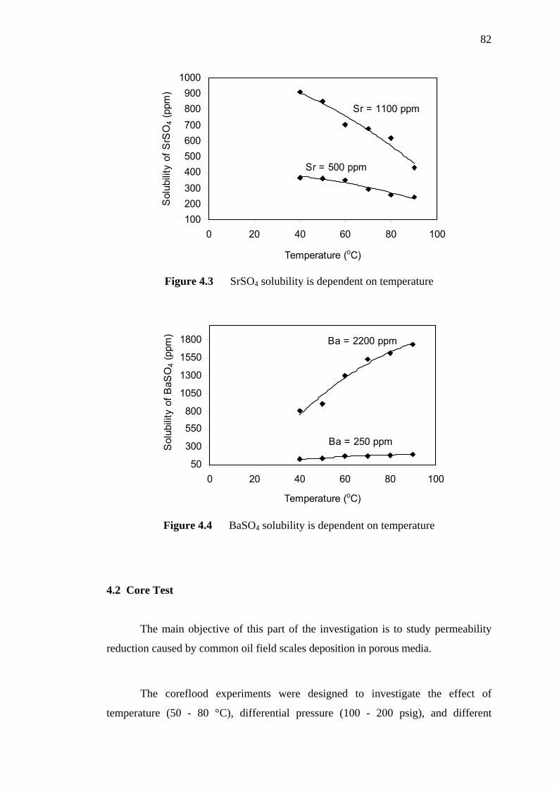
82

100200300400500600700800900

1000

0 20 40 60 80 10

Temperature (oC)

Sol

ubili

ty o

f SrS

O4

(ppm

)

0

Sr = 1100 ppm

Sr = 500 ppm

Figure 4.3 SrSO4 solubility is dependent on temperature

50

300

550

800

1050

1300

1550

1800

0 20 40 60 80 10

Temperature (oC)

Sol

ubili

ty o

f BaS

O4

(ppm

)

0

Ba = 2200 ppm

Ba = 250 ppm

Figure 4.4 BaSO4 solubility is dependent on temperature

4.2 Core Test

The main objective of this part of the investigation is to study permeability

reduction caused by common oil field scales deposition in porous media.

The coreflood experiments were designed to investigate the effect of

temperature (50 - 80 °C), differential pressure (100 - 200 psig), and different

83

concentrations of calcium, strontium, and barium ions (Table 3.2) on the scaling

tendency of brines.

During each run, the flow rate across the core was recorded continuously and

the permeability of core was calculated using Darcy’s linear-flow equation. This

decrease in flow rate only occurred during the experiments when supersaturated

brine was flowing through the cores. This confirms that the decrease is due to

precipitation of the calcium, strontium, and barium sulfates in the core with the

consequent reduction in its permeability and porosity. In the following, the results

for CaSO4, SrSO4, and BaSO4 experiments are discussed individually.

4.2.1 Calcium and Strontium Sulfates Experiments

In these experiments, the seawater was mixed with formation water within

the sandstone cores at temperatures (50 – 80 °C), differential pressure (100 - 200

psig), and different concentrations (7000 - 30000 ppm of Ca++ and 500 - 1100 ppm of

Sr++) of this study are given in tables (appendix C).

Typical results for flow rate and permeability reduction obtained were plotted

versus time and pore volumes of injected brine in Figures (4.5 - 4.25 and Appendix

E). In the following, extend of permeability damage, permeability decline trend, and

the results for various temperatures, concentrations, and differential pressure are

discussed individually.


Extend of permeability loss caused by CaSO4 and SrSO4 scaling in the rock

pores varied in different situations. Figure 4.5 shows the permeability change of a

less damaged core at temperature (50 °C) and differential pressure (100 psig); Figure

84

4.6 shows that of a severely damaged core after CaSO4 and SrSO4 scaling at

temperature (80 °C) and differential pressure (200 psig).

Nevertheless, about 4% - 14% permeability loss is observed in Figure (4.5), but

about 15% - 23% permeability reduction could occur in a heavily scaled core, as

Figure 4.6 indicates. The reduction in permeability might be caused due to crystals

blocking the pore throats as shown in the SEM view of Figure 4.49. The amount of

precipitation varied within the sandstone cores. The scale formation decreased as it

moves away from the formation water inlet part.

0.75

0.8

0.85

0.9

0.95

1

0 20 40 60 80 100 120Time (min)

Perm

eabi

lity

ratio

(Kd/

ki)

High salinity

Normal salinity ∆P = 100 psig T = 50 °C

Figure 4.5 Variation of permeability ratio as a function of time showing the effect

of concentration at 100 psig and 50 °C

85

0.75

0.8

0.85

0.9

0.95

1

0 20 40 60 80 100 120

Time (min)

Perm

eabi

lity

ratio

(Kd/

ki)

High salinity

Normal salinity

∆P = 200 psig T = 80 °C


of concentration at 200 psig and 80 °C


Figures 4.7 - 4.18 show the permeability decline trend changes with brine-

injection time. During the initial flow period, the permeability declined sharply soon

after the two waters mixed in the pores. The permeability decline then slowed and

gradually leveled out after the permeability decreased greatly. This phenomenon was

observed in all the core tests in which the scaling damage was severe. The same trend

was reported by Todd and Yuan (1992), Moghadasi et al. (2002), Moghadasi et al.

(2003b), Moghadasi et al. (2004a) and Ahmed (2004).


Temperature has a significant influence on solubility and crystal growth of

CaSO4 and SrSO4 is very important. To study its effect on the permeability

reduction, a set of tests were performed, where differential pressure and

concentration of calcium and strontium ions were kept constant and temperature was

varied.

86

Figures 4.7 - 4.12 and E.1 - 6 (Appendix E) show variation of flow rate and

permeability reduction with time at different temperatures. These figures show that

at higher temperatures the permeability declines more rapidly. This is because the

rate of precipitation increases with temperature. The increase in temperature also

causes a raise in supersaturation, because the solubility of CaSO4 and SrSO4 decrease

with temperature. This must have led to an increase of rate of precipitation and

consequently a faster permeability decline.

0.75

0.8

0.85

0.9

0.95

1

0 20 40 60 80 100 120

Time (min)

Per

mea

bilit

y ra

tio (K

d/ki

)

T = 50 °CT = 70 °CT = 80 °C

∆P = 100 psig Ca = 30000 ppm Sr = 1100 ppm


of temperature at 100 psig

87

0.75

0.8

0.85

0.9

0.95

1

0 20 40 60 80 100 120

Time (min)

Per

mea

bilit

y ra

tio (K

d/ki

)

T = 50 °CT = 70 °CT = 80 °C




0.75

0.8

0.85

0.9

0.95

1

0 20 40 60 80 100 120

Time (min)

Per

mea

bilit

y ra

tio (K

d/ki

)

T = 50 °CT = 70 °CT = 80 °C




88

0.85

0.9

0.95

1

0 20 40 60 80 100 120Time (min)

Per

mea

bilit

y ra

tio (K

d/ki

)

T = 50 °CT = 70 °CT = 80 °C


Figure 4.10 Variation of permeability ratio as a function of time showing the

effect of temperature at 100 psig

0.85

0.9

0.95

1

0 20 40 60 80 100 120Time (min)

Per

mea

bilit

y ra

tio (K

d/ki

)

T = 50 °CT = 70 °CT = 80 °C




89

0.85

0.9

0.95

1

0 20 40 60 80 100 120Time (min)

Per

mea

bilit

y ra

tio (K

d/ki

)

T = 50 °CT = 70 °CT = 80 °C





To investigate the effect of differential pressure on flow rate and permeability

reduction a number of tests were carried out. In these experiments, the concentration

of brine and temperature were kept constant and differential pressures are varied from

100 to 200 psig.

The variation of flow rate and permeability reduction with time at different

differential pressures are show in Figures 4.13 - 4.18 and E.7 – 12 (Appendix E).

From these figures, the permeability decline of porous medium is evident, even at

such low differential pressures.

The results illustrate that at low differential pressure, scale formation has

already as significant effect on the permeability decline as shown in Figures 4.13 and

4.16 for high and normal salinity respectively. As, the differential pressure was

increased, the rate of permeability decline becomes more rapid.

90

Moreover, at higher differential pressure more sulfate ions will pass through

the porous medium in a given interval of time. The supersaturation at the porous

medium will therefore increase the rate of precipitation. This increased precipitation

rate will produce a larger permeability decline as shown in Figures 4.15 and 4.18 for

high and normal salinity respectively. These results agreed with result by reported

by Moghadasi et al., (2002), Moghadasi et al., (2003b) and Moghadasi et al.,

(2004a).

Furthermore, the overall permeability of porous medium at high salinity

decreased to between 14% to 23% of initial permeability and normal salinity

between 4% - 15% of initial permeability depending on the differential pressure

used.

0.75

0.8

0.85

0.9

0.95

1

0 20 40 60 80 100 120Time (min)

Per

mea

bilit

y ra

tio (K

d/ki

)

∆P = 100 psig∆P = 150 psig∆P = 200 psig

T = 50 °C Ca = 30000 ppm Sr = 1100 ppm


effect of differential pressure at 50 °C

91

0.75

0.8

0.85

0.9

0.95

1

0 20 40 60 80 100 120Time (min)

Per

mea

bilit

y ra

tio (K

d/ki

)


T = 70 °C Ca = 30000 ppm Sr = 1100 ppm



0.75

0.8

0.85

0.9

0.95

1

0 20 40 60 80 100 120Time (min)

Per

mea

bilit

y ra

tio (K

d/ki

)


T = 80 °C Ca = 30000 ppm Sr = 1100 ppm



92

0.85

0.9

0.95

1

0 20 40 60 80 100 120Time (min)

Per

mea

bilit

y ra

tio (K

d/ki

)


T = 50 °C Ca = 7000 ppm Sr = 500 ppm



0.85

0.9

0.95

1

0 20 40 60 80 100 120Time (min)

Per

mea

bilit

y ra

tio (K

d/ki

)


T = 70 °C Ca = 7000 ppm Sr = 500 ppm



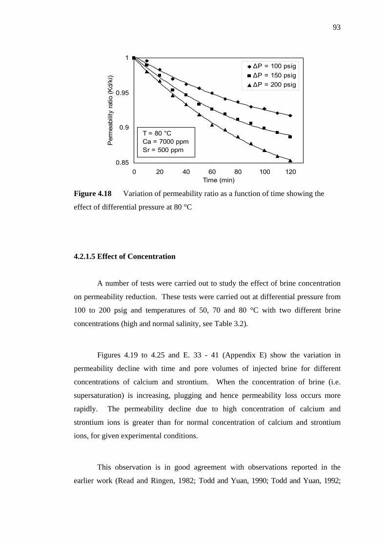
93

0.85

0.9

0.95

1

0 20 40 60 80 100 120Time (min)

Per

mea

bilit

y ra

tio (K

d/ki

)


T = 80 °C Ca = 7000 ppm Sr = 500 ppm




A number of tests were carried out to study the effect of brine concentration

on permeability reduction. These tests were carried out at differential pressure from

100 to 200 psig and temperatures of 50, 70 and 80 °C with two different brine

concentrations (high and normal salinity, see Table 3.2).

Figures 4.19 to 4.25 and E. 33 - 41 (Appendix E) show the variation in

permeability decline with time and pore volumes of injected brine for different

concentrations of calcium and strontium. When the concentration of brine (i.e.

supersaturation) is increasing, plugging and hence permeability loss occurs more

rapidly. The permeability decline due to high concentration of calcium and

strontium ions is greater than for normal concentration of calcium and strontium

ions, for given experimental conditions.

This observation is in good agreement with observations reported in the

earlier work (Read and Ringen, 1982; Todd and Yuan, 1990; Todd and Yuan, 1992;

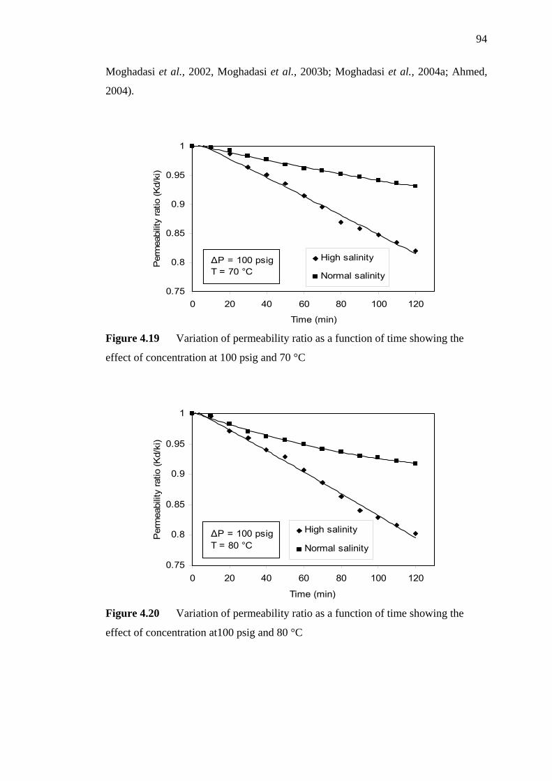
94

Moghadasi et al., 2002, Moghadasi et al., 2003b; Moghadasi et al., 2004a; Ahmed,

2004).

0.75

0.8

0.85

0.9

0.95

1

0 20 40 60 80 100 120

Time (min)

Per

mea

bilit

y ra

tio (K

d/ki

)

High salinity

Normal salinity

∆P = 100 psig T = 70 °C


effect of concentration at 100 psig and 70 °C

0.75

0.8

0.85

0.9

0.95

1

0 20 40 60 80 100 120

Time (min)

Per

mea

bilit

y ra

tio (K

d/ki

)

High salinity



effect of concentration at100 psig and 80 °C

95

0.75

0.8

0.85

0.9

0.95

1

0 20 40 60 80 100 120

Time (min)

Per

mea

bilit

y ra

tio (K

d/ki

)

High salinity



effect of concentration 150 psig and 50 °C

0.75

0.8

0.85

0.9

0.95

1

0 20 40 60 80 100 120

Time (min)

Per

mea

bilit

y ra

tio (K

d/ki

)

High salinity




96

0.75

0.8

0.85

0.9

0.95

1

0 20 40 60 80 100 120

Time (min)

Per

mea

bilit

y ra

tio (K

d/ki

)

High salinity

Normal salinity

∆P = 150 psig T = 80 °C



0.75

0.8

0.85

0.9

0.95

1

0 20 40 60 80 100 120

Time (min)

Per

mea

bilit

y ra

tio (K

d/ki

)

High salinity




97

0.75

0.8

0.85

0.9

0.95

1

0 20 40 60 80 100 120

Time (min)

Per

mea

bilit

y ra

tio (K

d/ki

)

High salinity

Normal salinity

∆P = 200 psig T = 70 °C



4.2.2 Barium Sulfate Experiments

The experimental procedure for scale formation with barium sulfate was

exactly the same as the procedure used for calcium and strontium sulfates

experiments.

A series of experiments was designed to investigate the effect of operating

parameters such as differential pressure (100 - 200 psig); temperature (50 – 80 °C)

and concentration (250 - 2200 ppm of Ba++) on barium sulfate scale formation as

given in tables (Appendix B).

The flow rate was measured in each run for time periods. Figures 4.26 to

4.46 and D.1 - 42 (Appendix D) show variation of the flow rate and permeability

decline as a function of time and pore volumes of injected brine. In the following,

extend of permeability damage, permeability decline trend and the results for various

temperatures, concentrations and differential pressure are discussed individually:

98


Extend of permeability loss caused by BaSO4 scaling in the rock pores varied

in different situations. Figure 4.26 shows the permeability change of a less damaged

core at temperature (80 °C) and differential pressure (100 psig); Figure 4.27 shows

that of a severely damaged core after BaSO4 scaling at temperature (50 °C) and

differential pressure (200 psig). About 5% - 12% permeability loss was observed in

Figure 4.26, but about 9%-19% initial permeability reduction occurred in a heavily

scaled core, as shown in Figure 4.27.

Moreover, the reduction in permeability is possibly caused by crystals

blocking the pore throats as shown by the SEM (Figure 4.48). The amount of

precipitation varied within the sandstone cores, there being more scale near the

formation water inlets and least scale was observed furthest from the inlet parts.

0.75

0.8

0.85

0.9

0.95

1

0 20 40 60 80 100 120Time (min)

Per

mea

bilit

y ra

tio (k

d/ki

)

∆P = 100 psig T = 80 °C

Ba = 250 ppm

Ba = 2200 ppm



99

0.75

0.8

0.85

0.9

0.95

1

0 20 40 60 80 100 120Time (min)

Per

mea

bilit

y ra

tio (K

d/ki

)

∆P = 200 psig T = 50 °C

Ba = 250 ppm

Ba = 2200 ppm




The overall core permeability with brine- injection time curves from all core

tests had concave shapes and shown in Figures 4.28 to 4.39. Even the final extend of

permeability reduction was small. Such permeability declined trends indicates that the

initial stage of scale formation resulted in fast permeability damage and that the

damage rate was significantly reduced after a certain period of scale deposition. This

phenomenon was observed in all the core tests in which the scaling damage was

severe. The same trend was reported by Todd and Yuan (1990) and Todd and Yuan

(1992).


The influence of temperature on the solubility and crystal growth of barium

sulfate is very important. To study its effect on the permeability reduction, a number

of experimental runs were carried out. In these experiments, the concentration of

100

brine and differential pressure were kept constant and temperatures were varied from

50 to 80 °C.

Figures 4.28 to 4.33 and D.22 - 27 (Appendix D) show the variation of

permeability reduction with time and pore volumes of injected brine at different

temperatures. These figures show that the effect of temperature on permeability

reduction. As temperature rises, the rate of nucleation and crystal growth and

plugging are decreased. Consequently in lower temperature, the rate of permeability

ratio reduction becomes faster.

Comparing the findings from the scale formation study at 50 °C in Figure

4.27 with those obtained from 80 °C experiments in Figure 4.26 reveals some aspects

of the effect of temperatures. The permeability decline is less rapid at higher

temperature, since the rate of precipitation decrease with temperature.

0.75

0.8

0.85

0.9

0.95

1

0 20 40 60 80 100 120Time (min)

Per

mea

bilit

y ra

tio (K

d/ki

)

T = 50 °CT = 70 °CT = 80 °C

∆P = 100 psig Ba = 2200 ppm



101

0.75

0.8

0.85

0.9

0.95

1

0 20 40 60 80 100 120Time (min)

Per

mea

bilit

y ra

tio (K

d/ki

)

T = 50 °CT = 70 °CT = 80 °C

∆P = 150 psig Ba = 2200 ppm



0.75

0.8

0.85

0.9

0.95

1

0 20 40 60 80 100 120Time (min)

Per

mea

bilit

y ra

tio (K

d/ki

)

T = 50 °CT = 70 °CT = 80 °C

∆P = 200 psig Ba = 2200 ppm



102

0.9

0.95

1

0 20 40 60 80 100 120Time (min)

Per

mea

bilit

y ra

tio (k

d/ki

)

T = 50 °CT = 70 °CT = 80 °C

∆P = 100 psig Ba = 250 ppm



0.9

0.95

1

0 20 40 60 80 100 120Time (min)

Per

mea

bilit

y ra

tio (K

d/ki

)

T = 50 °CT = 70 °CT = 80 °C

∆P = 150 psig Ba = 250 ppm



103

0.9

0.95

1

0 20 40 60 80 100 120Time (min)

Per

mea

bilit

y ra

tio (K

d/ki

)

T = 50 °CT = 70 °CT = 80 °C

∆P = 200 psig Ba = 250 ppm




To investigate the effect of injection differential pressure on flow rate and

permeability reduction, number of experimental runs were performed, in which the

concentration of barium ion and temperature were kept constant while the injection

differential pressure was varied in each test.

The variations of flow rate and permeability ratio as a function of time at

different differential pressures are shown in Figures 4.34 to 4.39 and D.7-12

(Appendix D). From these figures, the rates of permeability decreased sharply as the

differential pressure increased. The reason for this behavior may be due to the fact

that rate of plugging increases as differential pressure increases.

From the Figures 4.34 to 4.39 and D.7-12 (Appendix D), scale formation has

a significant effect on decrease in permeability even at such low differential pressure.

As, the differential pressure was increased, the rate of permeability declined more

rapidly. At higher differential pressures, more sulfate ions passed through the porous

medium in a given interval of time, hence providing more material for deposition.

104

This shows that by increases of differential pressure, the value of supersaturation

increased; consequently the rate of precipitation, crystal growth and plugging is

rapidly raised and sharply decrease in permeability ratio. This observation is in good

agreement with observations reported in previous studies (Todd and Yuan, 1990; Todd

and Yuan, 1992).

In these experiments, the overall permeability of porous medium at high

barium decreased to between 12% to 19% of initial permeability and normal barium

between 5% - 9% of initial permeability depending on the differential pressure used.

0.75

0.8

0.85

0.9

0.95

1

0 20 40 60 80 100 120Time (min)

Per

mea

bilit

y ra

tio (K

d/ki

)


T = 50 °C Ba = 2200 ppm



105

0.75

0.8

0.85

0.9

0.95

1

0 20 40 60 80 100 120Time (min)

Per

mea

bilit

y ra

tio (K

d/ki

)


T = 70 °C Ba = 2200 ppm



0.75

0.8

0.85

0.9

0.95

1

0 20 40 60 80 100 120Time (min)

Per

mea

bilit

y ra

tio (K

d/ki

)


T = 80 °C Ba = 2200 ppm



106

0.9

0.95

1

0 20 40 60 80 100 120Time (min)

Per

mea

bilit

y ra

tio (K

d/ki

)


T = 50 °C Ba = 250 ppm



0.9

0.95

1

0 20 40 60 80 100 120Time (min)

Per

mea

bilit

y ra

tio (K

d/ki

)


T = 70 °C Ba = 250 ppm



107

0.9

0.95

1

0 20 40 60 80 100 120Time (min)

Per

mea

bilit

y ra

tio (K

d/ki

)


T = 80 °C Ba = 250 ppm




To investigate the effect of brine concentration on permeability reduction and

flow rate a number of tests were considered, in which the differential pressure and

temperature was remained constant with two different brine concentrations (high and

normal barium, see Table 3.2).

Figures 4.40 to 4.50 and D.34 - 44 (Appendix D) show the variation in

permeability decline with time and pore volumes of injected brine for different

concentrations of barium. These figures show that the effect of concentration on

permeability ratio reduction. A concentration is increased the supersaturation of

brine raises and the rate of nucleation and crystal growth raised. Therefore by

increasing of concentration, the rate of reaction, nucleation, crystal growth and

plugging are increased.

Moreover, the permeability decline due to high concentration of barium ions

is greater than for normal concentration of barium ions, for given experimental

conditions. This observation is in good agreement with observations reported in the

108

earlier work (Read and Ringen, 1982; Mitchell et al., 1980; Todd and Yuan, 1990;

Todd and Yuan, 1992; Wat et al., 1992).

0.75

0.8

0.85

0.9

0.95

1

0 20 40 60 80 100 120Time (min)

Per

mea

bilit

y ra

tio (K

d/ki

)

∆P = 100 psig T = 50 °C

Ba = 250 ppm

Ba = 2200 ppm



0.75

0.8

0.85

0.9

0.95

1

0 20 40 60 80 100 120Time (min)

Per

mea

bilit

y ra

tio (K

d/ki

)

∆P = 150 psig T = 50 °C

Ba = 250 ppm

Ba = 2200 ppm



109

0.75

0.8

0.85

0.9

0.95

1

0 20 40 60 80 100 120Time (min)

Per

mea

bilit

y ra

tio (k

d/ki

)

∆P = 100 psig T = 70 °C

Ba = 250 ppm

Ba = 2200 ppm



0.75

0.8

0.85

0.9

0.95

1

0 20 40 60 80 100 120Time (min)

Per

mea

bilit

y ra

tio (k

d/ki

)

∆P = 150 psig T = 70 °C

Ba = 250 ppm

Ba = 2200 ppm



110

0.75

0.8

0.85

0.9

0.95

1

0 20 40 60 80 100 120Time (min)

Per

mea

bilit

y ra

tio (k

d/ki

)

∆P = 200 psig T = 70 °C

Ba = 250 ppm

Ba = 2200 ppm



0.75

0.8

0.85

0.9

0.95

1

0 20 40 60 80 100 120Time (min)

Per

mea

bilit

y ra

tio (k

d/ki

)

∆P = 150 psig T = 80 °C

Ba = 250 ppm

Ba = 2200 ppm



111

0.75

0.8

0.85

0.9

0.95

1

0 20 40 60 80 100 120Time (min)

Per

mea

bilit

y ra

tio (k

d/ki

)

∆P = 200 psig T = 80 °C

Ba = 250 ppm

Ba = 2200 ppm



0.75

0.8

0.85

0.9

0.95

1

0 20 40 60 80 100 120Time (min)

Perm

eabi

lity

ratio

(Kd/

ki)

High barium

High salinity

∆P = 200 psig T = 50 ºC



112

0.75

0.8

0.85

0.9

0.95

1

0 20 40 60 80 100 120Time (min)

Perm

eabi

lity

ratio

(Kd/

ki)

High barium

High salinity

∆P = 200 psig T = 80 ºC



0.75

0.8

0.85

0.9

0.95

1

0 20 40 60 80 100 120Time (min)

Perm

eabi

lity

ratio

(Kd/

ki)

High barium

High salinity

∆P = 100 psig T = 50 ºC



113

0.75

0.8

0.85

0.9

0.95

1

0 20 40 60 80 100 120Time (min)

Perm

eabi

lity

ratio

(Kd/

ki)

High barium

High salinity

∆P = 100 psig T = 80 ºC



4.3 Scanning Electron Microscopy Analysis

The scaled core samples were examined by SEM to observe the particle size

and morphology of the precipitates. The formation of CaSO4, SrSO4, and BaSO4

during flow of injection and formation waters in porous media have been observed by

Scanning Electron Microscopy (SEM) micrographs which shows CaSO4, SrSO4, and

BaSO4 crystals formation in porous space.

Figures 4.51 and 4.52 show SEM image of the CaSO4, SrSO4, and BaSO4

scaling crystals in rock pores precipitated from mixed seawater with formation water

inside the cores. Comparison of BaSO4 with CaSO4 and SrSO4 formed in porous

media did not show significant differences in crystal external morphology. The

differences line in the irregularity of crystals formed in rock pores and the crystal size

variations from one location to another in a core. The average size of BaSO4 crystals

precipitated from mixed brines was about 2.5 µm larger than the average size of

CaSO4 and SrSO4 crystals is about 1.8 µm.

114

In all core tests, the abundance of scale reduced significantly from the front of

the core to the rear indicating that scale formation in porous media was rapid with the

observation that the flow rate decreased soon after two incompatible waters were

mixed into a core. The observations of scaling sites from previous tests (Todd and

Yuan, 1990; Todd and Yuan, 1992; Ahmed, 2004) were confirmed by this test results.

In general, Figures 4.51 and 4.52 indicate that the front sections of a core

suffered considerable greater scaling damage. The reason the scaling decreased

downstream of a core is clear: most of the scaling ions had deposited within the front

sections as soon as they were mixed and left few ions to precipitate from the flow

stream in the rear sections. Figure 4.53 shows an SEM image of an unscaled core

samples.

(a) (b)

(c) (d)

Figure 4.51 SEM image of an unscaled sandstone cores

115

(a) (b)

(c) (d)

Figure 4.52 SEM image of BaSO4 scale in sandstone core at 200 psig and 50 °C

116

(a) (b)

(c) (d)

Figure 4.53 SEM image of CaSO4 and SrSO4scales in sandstone core at 200 psig

and 80 °C

CHAPTER 5

CONCLUSIONS AND RECOMMENDATIONS 5.1 Conclusions

The work carried out in this study focused on the effect of temperature,

concentration of brine, and differential pressure on permeability reduction by

deposition of scale formation in a porous medium and the solubility of scales

formed and how their solubilities were affected by changes in salinity and

temperature.

Coreflood tests with injected and formation waters at various sets of

conditions such as temperature, differential pressure and concentration gave the

following conclusions.

(1) The experimental results confirm the general trend in solubility dependencies

for common oil field scales, determined at various temperatures. A

temperature rise from 40 to 90 °C causes an increase in BaSO4 solubility and

a decrease of CaCO3, CaSO4, and SrSO4 solubilities.

(2) Laboratory coreflooding has demonstrated that in-situ precipitation of

calcium, strontium and barium sulfates occurs when synthetic seawater

containing sulfate is mixed in-situ with formation water that contains a

significant amount of dissolved calcium, strontium, and barium ions.

118

(3) This scale is expected to form when pressure maintenance by seawater

injection into the aquifer is started. More severe scaling by this material is to

be expected when seawater breakthrough into production wells.

(4) Permeability decline caused by CaSO4, SrSO4, and BaSO4 scale formation in

the porous media ranged from 4% to 23% of the initial permeability,

depending on brine composition, initial permeability, temperature,

differential pressure, and brine injection period.

(5) The worst permeability loss occurred in the porous media from 15% to 23%

of the initial permeability at temperature (80 °C) and differential pressure

(200 psig) for CaSO4 and SrSO4 experiments and from 9% to 19% of the

initial permeability at temperature (50 °C) and differential pressure (200 psig)

for BaSO4 experiments.

(6) CaSO4, SrSO4, and BaSO4 precipitates did not plug the sandstone cores to the

same extent. The experiments with CaSO4 and SrSO4 precipitates produced a

4% to 23% reduction in initial permeability. The experiments with BaSO4

precipitate produced a 5% to 19% reduction in initial permeability.

(7) The pattern of permeability decline in a porous medium due to scaling

injection was characterized by a concave curve with a steep initial decline

which gradually slowed down to a lower. The initial steepness of these

curves generally decreased with increasing distance from the point of mixing

of the incompatible brines. The concave shape of the permeability-time

curves was common to the majority of the porous medium flow tests.

(8) Several factors influencing scale formation had been examined. Increasing

temperature, concentration of brine (i.e. supersaturation), and differential

pressure had a detrimental effect on the permeability reduction.

(9) At higher temperatures, CaSO4 and SrSO4 scale is increased because the

solubilities of CaSO4 and SrSO4 decrease with temperature. This must have

increased the rate of precipitation and consequently the permeability decline.

119

(10) The permeability decline due to high concentration of calcium, strontium, and

barium ions is greater than for normal concentration of calcium, strontium

and barium ions, for given experimental conditions.

(11) The formation of CaSO4, SrSO4, and BaSO4 during flow of injection and

formation waters in porous media have been observed by Scanning Electron

Microscopy (SEM) micrographs show CaSO4, SrSO4, and BaSO4 crystals

formation in porous space.

5.2 Recommendations

Based on the results and conclusions obtained from this study, the following

suggestions for future work in the same area are recommended:

(1) Instead of synthetic brines, real oil field brines can be employed in the study

by mixing field disposal water and seawater.

(2) Scale build-up can be monitored by placing a multipressure tapped core

holder in a temperature oven and measuring the pressure drop along the core

during flooding.

(3) The concentrations of calcium, barium, and strontium in effluent sample

during coreflood experiments can be determined and much improved using

an in–line ion analyzer or some other analytical devices.

(4) The effect of residual oil saturation on the precipitation reaction can be

investigated.

120

REFERENCES Ahmed, J. S. (2004). Laboratory Study on Precipitation of Calcium Sulphate in Berea

Sand Stone Cores. King Fahd University of Petroleum & Minerals: M.E.

Thesis.

Allaga, A. D., Wu, G., Sharama, M. M. and Lake, W. L. (1992). Barium and Calcium

Sulfate Precipitation and Migration inside Sandpacks. SPE Formation

Evaluation. SPE19765:79 – 86.

Andersen, I. K., Halvorsen, E., Saelensminde, T. and Ostbye, O. N. (2000). Water

Management in a Closed Loop - Problems and Solutions at Brage Field.

The SPE European Petroleum Conference. October 24-25. Paris, France: SPE

65162, 1 – 12.

Asghari, K. and Kharrat, R. (1995). Alteration of Permeability by Fine Particle

Movement-A Water Injectivity Problem. The SPE International Symposium

on Oilfield Chemistry. February 14 – 17. San Antonio, Texas: SPE 29006,

655- 665.

Bagci, S., Kok, M.V. and Turksoy, U. (2000). Determination of Formation Damage

in Limestone Reservoirs and its Effect on Production. Journal of Petroleum

Science and Engineering. 28: 1–12

Bayona, G.H. (1993). A Review of Well Injectivity Performance in Saudi Arabia’s

Ghawar Field Seawater Injection Program. The SPE Middle East Oil

Technical Conference and Exhibition. April 3-6. Bahrain: SPE 25531, 201 –

214.

Bedrikovetsky, G. P. Moraes, P. G., Monteriro, R., Lopes, P. R., Rosario, F. F. and

Bezerra, C. M. (2005).Characterization of Sulphate Scaling Formation

121

Damage from Laboratory Measurements (To Predict Well-Productivity

Decline). The SPE fifth International Symposium on Oilfield Chemistry.

February 2 – 4. Texas, USA: SPE 93121, 1 – 14.

Bedrikovetsky, G. P., Mackay, E., Monteriro, P. R., Gladstone, M. P. and Rosario, F.

F. (2006). Laboratory and Field Prediction of Sulfate Scaling Damage. The

2006 SPE International Oilfield Scale Symposium. May 30 –1 June.

Aberdeen, UK: SPE 100611, 1 – 18.

Bertero, L., Chierici, L. G., Gottardi, G., Mesini, E. and Mormino, G. (1988).

Chemical Equilibrium Models: Their Use in Simulating the Injection of

Incompatible Waters. SPE Reservoir Engineering. February 1988, 288 –

294.

Bezemer, C. and Bauer, A. K. (1969). Prevention of Carbonate Scale Deposition: A

Well-Packing Technique with Controlled Volubility Phosphates. Journal of

Petroleum Technology. April 1969, 505 – 514.

Bezerra, M. C. M., Khali, N. C. and Rosario, F. F. (1990). Barium and Strontium

Sulfate Scale Formation due to Incompatible Water in the Namorado Field,

Campos Basin, Brazil. The SPE latten American production engineering

conference. October 14 – 18. Rio Janetro: SPE 21109, 1 – 5.

Brown, F. D. A., Merrett, J. S. and Putnam, S. J. (1991). Coil-Tubing milling/

Underreaming of Barium Sulphate Scale and Scale Control in the Forties

Field. The Offshore Europe Conference. September 3 – 6. Aberdeen: SPE

23106, 1 – 17.

Carlberg, L.B. and Matthews, R. R. (1973). Solubility of Calcium Sulfate in Brine.

The Oilfield Chemistry Symposium of the Society of Petroleum Engineers of

AIME. May 24-25. Denver, Colo: SPE 4353, 1-10.

Chen, T., Neville, A. and Yuan, M. (2004). Effect of PPCA and DETPMP Inhibitor

Blends on CaCO3 Scale Formation. The 6th International Symposium on

Oilfield Scale. May 26 – 27. Aberdeen, UK: SPE 87442, 1 –7.

122

Clemmit, F. A., Ballance, C. D. and Hunton, G. A. (1985). The Dissolution of Scales

in Oilfield Systems. The Offshore Europe 85 Conference in conjunction with

the Society of Petroleum Engineers of AIME. September 10 – 13. Aberdeen:

SPE 14010, 1 –32.

Collins, R. I. and Jordan, M. M. (2001). Occurrence, Prediction and Prevention of

Zinc Sulfide Scale within Gulf Coast and North Sea High Temperature/High

Salinity Production Wells. The SPE Third International Symposium on

Oilfield Scale. January 30 – 31. Aberdeen, UK: SPE 68317, 1 – 17.

Collins, R. I. and Jordan, M. M. (2003). Occurrence, Prediction and Prevention of

Zinc Sulfide Scale within Gulf Coast and North Sea High-Temperature and

High-Salinity fields. SPE Production and Facilities, August 2003. 200 – 209.

Collins, R. I. (2005). Predicting the Location of Barium Sulfate Scale Formation in

Production Systems. The SPE International Symposium on Oilfield Scale.

May 11 – 12. Aberdeen, UK: SPE 94366, 1 – 6.

Collins, R. I., Duncum, D.S., Jordan, M. M. and Feasey, D. N. (2006). The

Development of a Revolutionary Scale-Control Product for the Control of

Near-Well Bore Sulfate Scale within Production Wells by the Treatment of

Injection Seawater. The 2006 SPE Oilfield Scale Symposium. 31 May- 1 June.

Aberdeen, UK: SPE 100357, 1 – 20.

Connell, D. (1983). Prediction and Treatment of Scale in North Sea Fields. Heriot-

watt university : M.E. Thesis

Crowe, W. C. (1986). Precipitation of Hydrated Silica from Spent Hydrofluoric

Acid. Journal of Petroleum Technology. November 1986, 1234 – 1240.

El-Hattab, I. M. (1982). GUPCO’S Experience in Treating Gulf of Suez Seawater for

Waterflooding the El Morgan Oil Field. Journal of Petroleum Technology.

July 1982, 1449 – 1460.

123

Essel, J. A. and Carlberg, L. B. (1982). Strontium Sulfate Scale Control by Inhibitor

Squeeze Treatment in the Fatech Field. Journal of Petroleum Technology.

June 1982, 1302 – 1306.

Guimaraes, Z., Franca, B. A., Duque, H. L, Souza, D. B. R., Porto, M., Neves, D.

and Peixoto, C. (2007). Case Histories of Barium Sulfate Scale Removal in

Offshore Wells, Brazil, Using a New Engineered Combination of Coiled-

Tubing Tools. The 2007 SPE/ICOTA Coiled Tubing and Well Intervention

Conference and Exhibition. March 20 – 21. Texas, USA: SPE 107063, 1 – 8.

Jacques, F. D. and Bourland, I. B. (1983). A Study Solubility of Strontium Sulfate.

Society of Petroleum Engineers Journal. April 1983, 292 – 300.

Jordan, M. M. and Mackay, J. E. (2005). Integrated Field Development for Effective

Scale Control Throughout the Water Cycle in Deep Water Subsea Fields. The

SPE Europec/EAGE Annual Conference. June 13 – 16. Madrid, Spain: SPE

94052, 1 –9.

Jordan, M. M., Collins, R. I. and Mackay, J. E. (2006a). Low-Sulfate Seawater

Injection for Barium Sulfate Scale Control: A life-of-Field Solution to a

Complex Challenge. The 2006 SPE International Symposium and Exhibition

on Formation Damage Control. February 15 – 17. Lafayette, LA: SPE 98096,

1 – 23.

Jordan, M. M., Johnston, J. C. and Robb, M. (2006b). Evaluation Methods for

Suspended Solids and Produced Water as an Acid in Determining

Effectiveness of Scale Control Both Downhole and Topside. SPE Production

and operations. February 2006, 7 – 18.

Jordan, M. M., Graff, J. C. and Cooper, N. K. (2000). Development and Deployment

of a Scale Squeeze Enhancer and Oil-Soluble Scale Inhibitor To Avoid

Deferred Oil Production Losses During Squeezing Low-Water Cut Wells,

North Slope, Alaska. The 2000 SPE International Symposium on Formation

Damage Control. February 23 – 24. Lafayette, Louisiana: SPE 58725, 1 – 18.

124

Khatib, I. Z. (1994). Prediction of Formation Damage Due to Suspended Solids:

Modeling Approach of Filter Cake Buildup in Injectors. The SPE 89th

Annual Technical Conference and Exhibition. September 25 – 28. New

Orieans, USA: SPE 28488, 263 – 273.

Khelil, C., Harouaka, A. and Delhoume, A. (1979). Water Injection in Algeria-

Problems and Solutions. The Middle East Oil Technical Conference of the

Society of Petroleum Engineers. March 25-29. Manama, Bahrain: SPE 7762,

97 – 106.

Krueger, F. R. (1986). An Overview of Formation Damage and Well Productivity in

Oilfield Operations. Journal of Petroleum Technology. February 1986, 131 –

152.

Leone, A., J. and Scott, M., E. (1988). Characterization and Control of Formation

Damage during Water Flooding Of a High-Clay-Content Reservoir. SPE

Reservoir Engineering . November 1988, 1279 – 1286.

Lindlof, C. J. and Stoffer, G. K. (1983). Acase study of sea water injection

incompatibility. Journal of Petroleum Technology, July 1983 1256 – 1262.

Mackay, J. E. (2003). Modeling In-Situ Scale Deposition: The Impact of Reservoir

and Well Geometries and Kinetic Reaction Rates. SPE Production and

Facilities. February 2003, 45 – 56.

Mackay, J. E. (2005). Scale Inhibitor Application in Injection Wells to Protect

Against Damage to Production Wells: when does it work?. The SPE

European Formation Damage Conference. May 25 – 27. Scheveningen,

Netherlands: SPE 95022, 1 –9.

Mackay, J. E. and Jordan, M. M. (2005). Impact of Brine Flow and Mixing in the

Reservoir on Scale Control Risk Assessment and Subsurface Treatment

Options: Case Histories. Journal of Energy Resources Technology. 127: 201

– 213.

125

Mackay, J. E., Collins, R. I. and Jordan, M. M. (2003). PWRI: scale Formation Risk

Assessment and Management. The SPE 5th International Symposium on

Oilfield Scale. January 29 – 30. Aberdeen, UK: SPE 80385, 1 – 18.

Mazzollnl, I. E., Betero, L. and Truefltt, S. C. (1992). Scale Prediction and

LaboratoryEvaluation of BaSO4 Scale inhibitors for Seawater Flood in a

High-Barium Environment. SPE Production Engineering. SPE 20894, 186 –

192.

McElhiney, E. J., Sydansk, D. R., Benzel, M. W. and Davidson, B. K. (2001).

Determination of in-situ precipitation of barium sulfate during coreflooding.

The SPE third International Symposium on Oilfield scale. January 30–31.

Aberdeen, UK: SPE 68309, 1 – 11.

Mitchell, W. R., Grist, M. D. and Boyle, J. M. (1980). Chemical Treatments

Associated With North Sea Projects. Journal of Petroleum Technology: SPE

7880, 904 – 912.

Moghadasi, J., Jamialahmadi, M., Muller-Steinhagen, H., Sharif, A., Ghalambor, A.,

Izadpanah, R. M. and Motaie, E. (2003a). Scale Formation in Iranian Oil

Reservoir and Production Equipment during Water Injection. The 5th

International Oilfield Scale Symposium and Exhibition. January 29 – 30.

Aberdeen, UK: SPE 80406, 1 – 14.

Moghadasi, J., Jamialahmadi, M., Muller-Steinhagen, H.and Sharif, A. (2003b).

Scale Formation in Oil Reservoir and Production Equipment during Water

Injection (Kinetics of CaCO4 and CaCO3 Crystal Growth and Effect on

Formation Damage). The SPE European Formation Damage Conference.

May 13 – 14. Hague, Netherlands: SPE 82233, 1 –12.

Moghadasi, J., Jamialahmadi, M., Muller-Steinhagen, H., Sharif, A., Izadpanah, R.

M., Motaie, E. and Barati, R. (2002). Formation Damage in Iranian Oil

Fields. The SPE International Symposium and Exhibition on Formation

Damage control. February 20 – 21. Lafayette, Louisiana: SPE 73781, 1 – 9.

126

Moghadasi, J., Muller-Steinhagen, H., Jamialahmadi, M. and Sharif, A (2004a).

Model study on the kinetics of oil field formation damage due to salt

precipitation from injection. Journal of Petroleum Science and Engineering.

43: 201– 217.

Moghadasi, J., Jamialahmadi, M., Muller-Steinhagen, H., Sharif, A. (2004b).

Formation Damage Due to Scale Formation in Porous Media Resulting From

Water Injection. The SPE International Symposium and Exhibition on

Formation Damage control. February 18-20. Lafayette, Louisiana: SPE

86524, 1 – 11.

Nancollas, H. G. and Liu, T. S. (1975). Crystal Growth and Dissolution of Barium

Sulfate. Society of Petroleum Engineers Journal. December 1975, 509 – 516.

Nasr-El-Din, A. H. (2003). New Mechanisms of Formation Damage: Lab Studies and

Case Histories. The SPE European Formation Damage Conference. May 13 –

14. Hague, Netherlands: SPE 82253, 1 –12.

Nasr-El-Din, A. H. and Al-Humaidan, Y. A. (2001). Iron Sulfide Scale: Formation,

Removal and Prevention. The 2001 SPE International Symposium on Oilfield

Scale. January 30 – 31. Aberdeen, UK: SPE 68315, 1 – 13.

Nasr-El-Din, A. H. Raju, U. K., Hilab, V. V. and Esmail J. O. (2004). Injection of

Incompatible Water as a Means of Water Shut-Off. The 6th SPE International

Symposium on Oilfield Scale. May 26- 27. Aberdeen, UK: SPE 87455, 1 –

13.

Nassivera, M. and Essel, A. (1979). Fateh field sea water injection – Water

Treatment, Corrosion, And scale control. The Middle East Oil Technical

Conference of the Society of petroleum Engineers. March 25 – 29. Manama,

Bahrain: SPE 7765, 133 – 138.

Oddo, E. J. and Tomson, B. M. (1994). Why Scale Forms and How to Predict It.

SPE Production and Facilities. February 1994, 47 – 54.

127

Oddo, E. J., Smith, P. J. and Tomason, B. M. (1991). Analysis of and Solutions to the

CaCO3 and CaSO4 Scaling Problems Encountered in Wells Offshore

Indonesia. The 66th Annual Technical Conference and Exhibition of the

Society of Petroleum Engineering. October 6 – 9. Dallas, TX: SPE 22782, 1 –

10.

Paulo, J., Mackay, J. E., Menzies, N. and Poynton, N. (2001). Implications of Brine

Mixing in the Reservoir for Scale Management in the Alba Field. The 2001

SPE International Symposium on Oilfield scale. January 30 – 31. Aberdeen,

UK: SPE 68310, 1 – 13.

Raju, U. K., Nasr-El-Din, A. H. and Al-Shafai, A. T. (2003). A Feasibility Study of

Mixing Disposal Water with Aquifer Water for Downhole Injection. The SPE

13th Middle East Oil Show and Conference. April 5 – 8. Bahrain: SPE 81449,

1 –9.

Read, A. P. and Ringen, K. J. (1982). The Use of Laboratory Tests to Evaluate

Scaling Problems during Water Injection. The SPE Sixth International

Symposium on Oilfield and Geothermal Chemistry. January 25 – 27. Dallas,

Texas: SPE 10593, 7 – 17.

Romero, C., Bazin, B., Zaitoun, A. and Leal-Calderon, F. (2007). Behavior of a

Scale Inhibitor Water-in-Oil Emulsion in Porous Media. SPE Production and

Operations. May 2007, 191 – 201.

Rousseau, G., Hurtevent, C., Azaroual, M., Kervevan, C. and Durance, V. M.

(2003). Application of a Thermo-Kinetic Model to the Prediction of

Scale in Angola Block 3 Field. The 5th International Oilfield Scale

Symposium. January 29 – 30. Aberdeen, UK: SPE 80387, 1 –8.

Salman, M. Al-Hashem, A. and Carew, J. (1999). Prediction of Scaling for the

Seawater Injection System at the Northern Kuwaiti Oil Fields. The 1999 SPE

Middle East Oil Show. February 20 – 23. Bahrain: SPE 53268, 1 –5.

128

Shen, J. and Corsby, C.C. (1983). Insight into Strontium and Calcium Sulfate Scaling

Mechanisms in a Wet Producer. Journal of Petroleum Technology. SPE

10597, 1249 – 1255.

Shuler, J. P., Freitas, A. E. and Bowker, A. K. (1991). Selection and Application of

BaSO4 Scale Inhibitors for a CO2 Flood, Rangely Weber Sand Unit,

Colorado. Society of Petroleum Engineers. SPE 18973, 1 – 8.

Smith, P.S., Clement Jr. C.C., and Mendoza Rojas, A. (2000). Combined Scale

Removal and Scale Inhibition Treatments. The 2000 second International

Symposium on Oilfield Scale. January 26 – 27. Aberdeen, UK: SPE 60222, 1

–6.

Stalker, R., Collins, R. I. and Graham, M. G. (2003). The Impact of Chemical

Incompabilities in Commingled Fluids on the Efficiency of a Produced Water

Reinjection System: A North Sea Example. The SPE International

Symposium on Oilfield chemistry. February 5 –7. Houston, Texas: SPE

80257, 1 –13.

Strachan, J. C., Heath, M.S., White, K., Williams, G., Strong, A. and Bell, K. (2004).

Experience With Pre-Emptive Squeeze Treatments on BM Magnus with

Aqueous Based Scale Inhibitors. The sixth International Symposium on

Oilfield Scale. May 26 – 27. Aberdeen, UK: SPE 87462, 1 – 13.

Sverjensky, A. D. (1984). Oilfield Brines As Ore-Forming Solutions. Economic

Geology and the Bulletion of Society of Economic Geologists. 79(1): 23 – 37.

Tahmasebi, A. H., Kharrat, R. and Masoudi, R. (2007). Prediction of Permeability

Reduction Rate Due To Calcium Sulfate Scale Formation in Porous Media.

The 15th SPE Middle East Oil and Gas Show and Conference. March 11 – 14.

Bahrain: SPE 105105, 1 –6.

Thomas, G. L., Albertsen, M., Perdeger, A., Knoke, K. H.H., Horstmann, W. B. and

Schenk, D. (1995). Chemical Characterization of Fluids and Their Modeling

With Respect to Their Damage Potential in Injection on Production Processes

129

Using an Expert System. The SPE International Symposium on Oilfield

Chemistry. February 14 – 17. San Antonio, U.S.A.: SPE 28981, 1 – 10.

Todd, C. A. and Yuan, D. M. (1990). Barium and Strontium Sulfate Solid-Solution

Formation in Relation to North Sea Scaling Problems. SPE Production

Engineering. August 1990, 279 – 285.

Todd, C. A. and Yuan, D. M. (1992). Barium and Strontium Sulfate Solid-Solution Scale

Formation at Elevated Temperatures. SPE Production Engineering. SPE 19762:

85 – 92.

Vetter, J. O., Farone, A. W., Veith, E. and Lankford, S. (1987). Calcium Carbonate

Scale Considerations: A Practical Approach. The SPE production Technology

Symposium. November 16 – 17. Lubbock, Texas: SPE 17009, 1 – 14.

Vetter, J. O., Kandarpa, V. and Harouaka, A. (1982). Prediction of Scale Problems

Due To Injection of Incompatible Waters. Journal of Petroleum Technology.

February 1982, 273 – 284.

Voloshin, I. A., Ragulin, V. V., Tyabayeva, E. N., Diakonov, I. I. and Mackay, J. E.

(2003). Scaling Problems in Western Siberia. The SPE fifth International

Symposium on Oilfield scale. January 29 – 30. Aberdeen, UK: SPE 80407, 1

– 8.

Wat, S. M. R., Sorbie, S. K., Todd, C. A., Chen, P. and Jiang, P. (1992). Kinetics of

BaSO4 Crystal Growth and Effect in Formation Damage. The SPE

International Symposium on Formation Damage control. February 25 – 27.

Lafayette, Louisiana: SPE 23814, 429 – 437.

Yeboah, D. Y., Somuah, K. S. and Saeed, R. M. (1993). Anew and Reliable Model

for Predicting Oilfield Scale Formation. The SPE International Symposium

on Oilfield Chemistry. March 2 – 5. New Orieans, U.S.A.: SPE 25166, 1 –

10.

Yuan, D. M. and Todd, C. A. (1991). Prediction of Sulfate Scaling Tendency in

Oilfield Operations. SPE production Engineering. SPE 18484: 63 – 72.

130

Zhang, Y. and Farquhar, R. (2001). Laboratory Determination of Calcium Carbonate

Scaling Rates for Oilfield Wellbore Environments. The 2001 SPE

International Symposium on Oilfield Scale. January 30 – 31. Aberdeen, UK:

SPE 68329, 1 –7.

131

APPENDICES

132

APPENDIX A

SUMMARY OF PREVIOUS EXPERIMENTAL WORKS

No. Study Rock Scale concentration Temp. Press. Flow rate 1 Mitchell et al.,

(1980) Sand pack barium

sulfate and calcium

carbonate

Sea water (ppm)

See table

A.2

Formation water (ppm)

See table A.1

20 - 90 ºC

4 – 40 psig

1:10

2 Read and Ringen, (1982)

Glass beads and in

synthetic alumina cores

barium, strontium, calcium,

sulfates and calcium

carbonate

Sea water (ppm)

See table

A.2


See table A.1

20 -70 ºC

1 - 22 Psig

2 ml / min

3 Lindlof and Stoffer, (1983)

Arab – D core ( Saudi Arabia)

Strontium and calcium sulfates

Sea water (ppm)

See table A.2


See table A.1

- - -

4 Bezerra et al.,(1990)

Sand stone Out crop (Brazil)

barium, and strontium sulfates

Sea water (ppm)

See table

A.2


See table A.1

80 °C

- 0.5 – 1.0 ml/min

ion (ppm) Ca 280 – 20000

5 Allaga et al., (1992)

Sand pack calcium and barium sulfates

Ba 1332 - 2746

- - 0.2 ml / min

6 Todd and Yuan, (1992)

Sand stone Clashach

barium, and strontium sulfates

Sea water (ppm)

See table

A.2


See table A.1

20- 70 ºC

1 – 2 Psig

7.5 ml / min

133

(Continued)

No. Study Rock Scale concentration Temp. Press. Flow rate 7 Wat et at.,

(1992) Sand pack Barium

sulfate Sea water

(ppm)

See table A.2


See table A.1

- - 0.5 ml/min

8 McElhiney et al., (2001)

Berea Sand stone

barium, strontium

and calcium sulfates

Sea water (ppm)

See table

A.2


See table A.1

21 ºC

14.7 Psig

-

9 Moghadasi et al. (2002)

Sand pack and

Glass beads

barium, strontium

and calcium sulfates

Sea water (ppm)

See table

A.2


See table A.1

25 – 80 °C

1 – 145 psig

1- 200 ml/min

ion (ppm) Ca 1770 -

13000 SO4 2600 – 7800

10 Moghadasi et al. (2003b)

Sand pack and

Glass beads

calcium and sulfate/

carbonate ions

CO3 800 –1060

50 – 80 °C

17.7 psig

25 – 100 ml/min

ion (ppm) Ca 2180 - 4175

11 AHMED, J. S. (2004)

Berea Sand stone

calcium sulfate

SO4 1200 - 2400

45 – 95 °C

100 -3000 psig

0.12 – 15 ml/min

12 Strachan et at. (2004)

BP Magnus core material

Barium and strontium,

sulfate

Sea water (ppm)

See table

A.2


See table A.1

116 °C

1500 psig 1 ml/min

ion (ppm) Ca 1770 -

13000 SO4 2600 – 7800

13 Moghadasi et al. (2004a)

Sand pack and

Glass beads

calcium and sulfate/

carbonate ions

CO3 800 –1600

50 – 80 °C

17.7 psig

25 – 100 ml/min

14 Bedrikovetsky et al., (2005)

Out crop RB (Brazil)

Barium sulfate

Sea water (ppm)

See table

A.2


See table A.1

- - -

15 Current Study 2006

Sandstone (Malaysia)

Calcium, strontium

and barium sulfates

Sea water (ppm)

See table

3.2


See table 3.2

50 – 80 °C

100 - 200 psig

-

134

Table A.1: Ions of Formation Water

Study Mitchell et al., (1980)

Read and

Ringen, (1982)

Lindlof and Stoffer, (1983)

Bezerra et al.

(1990)

Todd and Yuan, (1992)

Wat et at.,

(1992)

McElhiney et al., (2001)

Moghadasi et al. (2002)

Strachan et at.

(2004)

Bedrikovetsky et al., (2005)

Place Forties(North

sea)

(North sea)

Low- salinity Arab-D

High - salinity Arab-D

Namorado field (Brazil)

M (North

sea)

ST (North

sea)

(North sea)

West African FW Mishrif in Iranian

Magnus FW (North

sea)

Field N (Brazil)

Ca 3110 1100 13574 29760 2760 2809 779 2800 4000 4000 7920 250 -Ba 250 210 8 10 229 252 2180 250 240 0 18 220 229Sr 660 230 557 1035 415 574 369 575 230 230 610 45 -

SO4 0 <1 404 108 14 11 5 - 16 16 340 0 -HCO3 360 250 369 351 837 496 2140 - - - 244 1100 -

Na 30200 15200 29680 51187 33500 29370 41900 29400 37719 37719 43700 11065 38249K 430 380 - - 554 372 1700 370 46 46 - 210 -

Mg 480 110 1575 4264 374 504 102 500 873 873 2010 40 -Cl 53000 28000 73861 143285 59100 52360 68000 52647 68083 67959 86900 17350 59098

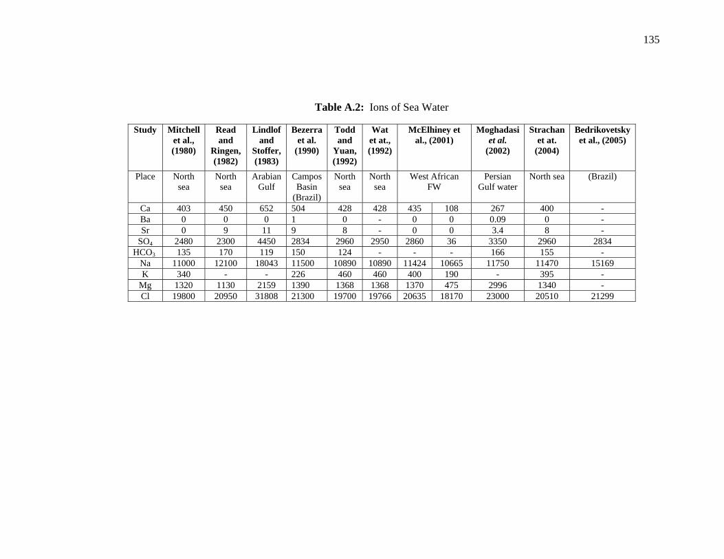
135

Table A.2: Ions of Sea Water

Study Mitchell et al., (1980)

Read and

Ringen, (1982)

Lindlof and

Stoffer, (1983)

Bezerra et al.

(1990)

Todd and

Yuan, (1992)

Wat et at., (1992)

McElhiney et al., (2001)

Moghadasi et al.

(2002)

Strachan et at.

(2004)

Bedrikovetsky et al., (2005)

Place Northsea

North sea

Arabian Gulf

Campos Basin

(Brazil)

North sea

North sea

West African FW

Persian Gulf water

North sea (Brazil)

Ca 403 450 652 504 428 428 435 108 267 400 -Ba 0 0 0 1 0 - 0 0 0.09 0 -Sr 0 9 11 9 8 - 0 0 3.4 8 -

SO4 2480 2300 4450 2834 2960 2950 2860 36 3350 2960 2834HCO3 135 170 119 150 124 - - - 166 155 -

Na 11000 12100 18043 11500 10890 10890 11424 10665 11750 11470 15169K 340 - - 226 460 460 400 190 - 395 -

Mg 1320 1130 2159 1390 1368 1368 1370 475 2996 1340 -Cl 19800 20950 31808 21300 19700 19766 20635 18170 23000 20510 21299

136

APPENDIX B

EXPERIMENTAL DATA AND RESULTS OF BARIUM SULFATE

Table B.1: Density and viscosity of formation water at room temperature

Normal salinity

formation water

High salinity

formation water

Normal barium

formation water

High barium

formation water

Sea water

Density (gm/ml)

1.11 1.15 1.07 1.10 1.01

Viscosity (cp)

1.70 1.83 1.53 1.61 -

Table B.2: Viscosity of sea water

Temperature (°C)

Viscosity of sea water (cp)

50 1.37 70 1.06 80 0.95

137

Table B.3: Experimental data of core flood at high barium: Run # 1

Injected

Time (min)

No. of PV’s

injected

Q

(cc/min)

T

(°C)

∆P

(psig)

D

(in)

L

(in)

Kd

(md)

Ki

(md)

kd/ki

10 2.24 10.01 50 100 1 3 12.70 12.76 0.995520 4.39 9.60 50 100 1 3 12.11 12.76 0.949030 6.51 9.46 50 100 1 3 11.93 12.76 0.935040 8.60 9.34 50 100 1 3 11.78 12.76 0.923350 10.68 9.30 50 100 1 3 11.73 12.76 0.919260 12.74 9.20 50 100 1 3 11.61 12.76 0.910170 14.78 9.12 50 100 1 3 11.51 12.76 0.901880 16.02 9.00 50 100 1 3 11.34 12.76 0.889090 18.77 8.81 50 100 1 3 11.12 12.76 0.8714100 20.71 8.67 50 100 1 3 10.94 12.76 0.8575110 22.64 8.59 50 100 1 3 10.84 12.76 0.8493120 24.56 8.55 50 100 1 3 10.79 12.76 0.8454


Injected

Time (min)

No. of PV’s

injected

Q

(cc/min)

T

(°C)

∆P

(psig)

D

(in)

L

(in)

Kd

(md)

Ki

(md)

kd/ki

10 3.06 15.91 50 150 1 3 13.38 13.46 0.994320 5.97 15.12 50 150 1 3 12.72 13.46 0.945030 8.83 14.87 50 150 1 3 12.51 13.46 0.929540 11.68 14.81 50 150 1 3 12.46 13.46 0.926050 14.5 14.66 50 150 1 3 12.33 13.46 0.916060 17.30 14.54 50 150 1 3 12.23 13.46 0.909070 20.04 14.27 50 150 1 3 12.00 13.46 0.891080 22.73 14.00 50 150 1 3 11.78 13.46 0.875090 25.38 13.77 50 150 1 3 11.58 13.46 0.8600100 28.00 13.61 50 150 1 3 11.45 13.46 0.8510110 30.58 13.39 50 150 1 3 11.26 13.46 0.8362120 33.14 13.30 50 150 1 3 11.19 13.46 0.8310

138


Injected

Time (min)

No. of PV’s

injected

Q

(cc/min)

T

(°C)

∆P

(psig)

D

(in)

L

(in)

Kd

(md)

Ki

(md)

kd/ki

10 4.85 21.29 50 200 1 3 13.43 13.52 0.993420 9.43 20.13 50 200 1 3 12.70 13.52 0.939030 13.95 19.83 50 200 1 3 12.51 13.52 0.925040 18.44 19.72 50 200 1 3 12.44 13.52 0.920050 22.90 19.60 50 200 1 3 12.36 13.52 0.914260 27.30 19.31 50 200 1 3 12.18 13.52 0.901070 31.64 19.05 50 200 1 3 12.02 13.52 0.889280 35.87 18.58 50 200 1 3 11.72 13.52 0.867190 40.06 18.40 50 200 1 3 11.61 13.52 0.8584100 44.19 18.14 50 200 1 3 11.44 13.52 0.8461110 48.22 17.69 50 200 1 3 11.16 13.52 0.8252120 52.19 17.41 50 200 1 3 10.98 13.52 0.8120


Injected

Time (min)

No. of PV’s

injected

Q

(cc/min)

T

(°C)

∆P

(psig)

D

(in)

L

(in)

Kd

(md)

Ki

(md)

kd/ki

10 2.23 12.67 70 100 1 3 12.37 12.40 0.997520 4.38 12.19 70 100 1 3 11.90 12.40 0.959530 6.50 12.02 70 100 1 3 11.73 12.40 0.946240 8.60 11.91 70 100 1 3 11.62 12.40 0.937450 10.67 11.75 70 100 1 3 11.47 12.40 0.925360 12.74 11.72 70 100 1 3 11.44 12.40 0.922370 14.79 11.62 70 100 1 3 11.34 12.40 0.914680 16.82 11.53 70 100 1 3 11.25 12.40 0.907290 18.82 11.32 70 100 1 3 11.05 12.40 0.8912100 20.80 11.21 70 100 1 3 10.94 12.40 0.8823110 22.76 11.10 70 100 1 3 10.83 12.40 0.8731120 24.71 11.04 70 100 1 3 10.78 12.40 0.8694

139


Injected

Time (min)

No. of PV’s

injected

Q

(cc/min)

T

(°C)

∆P

(psig)

D

(in)

L

(in)

Kd

(md)

Ki

(md)

kd/ki

10 3.67 20.42 70 150 1 3 13.29 13.34 0.996420 7.19 19.62 70 150 1 3 12.77 13.34 0.957230 10.66 19.34 70 150 1 3 12.52 13.34 0.938740 14.08 19.06 70 150 1 3 12.40 13.34 0.930150 17.47 18.89 70 150 1 3 12.29 13.34 0.921260 20.84 18.76 70 150 1 3 12.21 13.34 0.915470 24.19 18.64 70 150 1 3 12.13 13.34 0.909480 27.47 18.27 70 150 1 3 11.89 13.34 0.891390 30.72 18.10 70 150 1 3 11.78 13.34 0.8832100 33.94 17.95 70 150 1 3 11.68 13.34 0.8756110 37.12 17.70 70 150 1 3 11.52 13.34 0.8639120 40.28 17.58 70 150 1 3 11.44 13.34 0.8572


Injected

Time (min)

No. of PV’s

injected

Q

(cc/min)

T

(°C)

∆P

(psig)

D

(in)

L

(in)

Kd

(md)

Ki

(md)

kd/ki

10 5.34 25.06 70 200 1 3 12.23 12.30 0.994720 10.43 23.85 70 200 1 3 11.64 12.30 0.946330 15.43 23.44 70 200 1 3 11.44 12.30 0.930140 20.40 23.32 70 200 1 3 11.38 12.30 0.925350 25.34 23.17 70 200 1 3 11.31 12.30 0.919360 30.22 22.89 70 200 1 3 11.17 12.30 0.908270 35.03 22.58 70 200 1 3 11.02 12.30 0.896080 39.76 22.17 70 200 1 3 10.82 12.30 0.879490 44.41 21.80 70 200 1 3 10.64 12.30 0.8647100 48.99 21.47 70 200 1 3 10.48 12.30 0.8523110 53.53 21.31 70 200 1 3 10.40 12.30 0.8457120 58.03 21.10 70 200 1 3 10.30 12.30 0.8374

140


Injected

Time (min)

No. of PV’s

injected

Q

(cc/min)

T

(°C)

∆P

(psig)

D

(in)

L

(in)

Kd

(md)

Ki

(md)

kd/ki

10 2.68 14.66 80 100 1 3 12.83 12.85 0.998520 5.28 14.21 80 100 1 3 12.43 12.85 0.967530 7.84 14.01 80 100 1 3 12.26 12.85 0.953940 10.38 13.87 80 100 1 3 12.14 12.85 0.945050 12.88 13.69 80 100 1 3 11.98 12.85 0.932360 15.38 13.66 80 100 1 3 11.95 12.85 0.929870 17.87 13.60 80 100 1 3 11.90 12.85 0.925780 20.33 13.47 80 100 1 3 11.79 12.85 0.917590 22.76 13.28 80 100 1 3 11.62 12.85 0.9042100 25.16 13.11 80 100 1 3 11.47 12.85 0.8925110 27.53 12.99 80 100 1 3 11.37 12.85 0.8845120 29.88 12.87 80 100 1 3 11.26 12.85 0.8763


Injected

Time (min)

No. of PV’s

injected

Q

(cc/min)

T

(°C)

∆P

(psig)

D

(in)

L

(in)

Kd

(md)

Ki

(md)

kd/ki

10 4.25 21.70 80 150 1 3 12.66 12.70 0.997220 8.35 20.91 80 150 1 3 12.20 12.70 0.960330 12.39 20.61 80 150 1 3 12.02 12.70 0.946540 16.40 20.45 80 150 1 3 11.93 12.70 0.939450 20.36 20.21 80 150 1 3 11.79 12.70 0.928760 24.29 20.04 80 150 1 3 11.69 12.70 0.920570 28.21 19.97 80 150 1 3 11.65 12.70 0.917380 32.07 19.71 80 150 1 3 11.50 12.70 0.905290 35.89 19.49 80 150 1 3 11.37 12.70 0.8949100 39.65 19.17 80 150 1 3 11.18 12.70 0.8802110 43.39 19.08 80 150 1 3 11.13 12.70 0.8767120 47.10 18.91 80 150 1 3 11.03 12.70 0.8683

141


Injected

Time (min)

No. of PV’s

injected

Q

(cc/min)

T

(°C)

∆P

(psig)

D

(in)

L

(in)

Kd

(md)

Ki

(md)

kd/ki

10 5.68 28.14 80 200 1 3 12.31 12.36 0.995720 11.11 26.90 80 200 1 3 11.77 12.36 0.952130 16.46 26.49 80 200 1 3 11.59 12.36 0.938140 21.78 26.31 80 200 1 3 11.51 12.36 0.931250 27.05 26.10 80 200 1 3 11.42 12.36 0.923660 32.28 25.90 80 200 1 3 11.33 12.36 0.917070 37.46 25.62 80 200 1 3 11.21 12.36 0.906980 42.55 25.21 80 200 1 3 11.03 12.36 0.892190 47.57 24.87 80 200 1 3 10.88 12.36 0.8804100 52.54 24.62 80 200 1 3 10.77 12.36 0.8713110 57.43 24.20 80 200 1 3 10.59 12.36 0.8572120 62.27 23.95 80 200 1 3 10.48 12.36 0.8483

Table B.12: Experimental data of core flood at normal barium: Run # 10

Injected

Time (min)

No. of PV’s

injected

Q

(cc/min)

T

(°C)

∆P

(psig)

D

(in)

L

(in)

Kd

(md)

Ki

(md)

kd/ki

10 1.89 10.92 50 100 1 3 13.81 13.84 0.997820 3.76 10.85 50 100 1 3 13.69 13.84 0.989230 5.62 10.75 50 100 1 3 13.56 13.84 0.980140 7.47 10.71 50 100 1 3 13.51 13.84 0.976550 9.31 10.64 50 100 1 3 13.42 13.84 0.969460 11.13 10.53 50 100 1 3 13.29 13.84 0.960370 12.94 10.46 50 100 1 3 13.19 13.84 0.953280 14.73 10.39 50 100 1 3 13.11 13.84 0.947690 16.51 10.33 50 100 1 3 13.03 13.84 0.9412100 18.29 10.30 50 100 1 3 12.99 13.84 0.9385110 20.06 10.26 50 100 1 3 12.94 13.84 0.9353120 21.82 10.21 50 100 1 3 12.88 13.84 0.9305

142


Injected

Time (min)

No. of PV’s

injected

Q

(cc/min)

T

(°C)

∆P

(psig)

D

(in)

L

(in)

Kd

(md)

Ki

(md)

kd/ki

10 2.95 16.11 50 150 1 3 13.55 13.60 0.996120 5.88 15.98 50 150 1 3 13.44 13.60 0.987930 8.78 15.83 50 150 1 3 13.31 13.60 0.978840 11.66 15.74 50 150 1 3 13.24 13.60 0.973650 14.53 15.65 50 150 1 3 13.16 13.60 0.967560 17.36 15.47 50 150 1 3 13.01 13.60 0.956970 20.17 15.36 50 150 1 3 12.92 13.60 0.949780 22.96 15.22 50 150 1 3 12.80 13.60 0.941390 25.73 15.15 50 150 1 3 12.74 13.60 0.9364100 28.49 15.05 50 150 1 3 12.66 13.60 0.9309110 31.24 14.99 50 150 1 3 12.59 13.60 0.9256120 33.97 14.90 50 150 1 3 12.53 13.60 0.9211


Injected

Time (min)

No. of PV’s

injected

Q

(cc/min)

T

(°C)

∆P

(psig)

D

(in)

L

(in)

Kd

(md)

Ki

(md)

kd/ki

10 4.74 21.61 50 200 1 3 13.63 13.70 0.994920 9.44 21.43 50 200 1 3 13.52 13.70 0.987230 14.09 21.21 50 200 1 3 13.38 13.70 0.976940 18.71 21.07 50 200 1 3 13.29 13.70 0.970250 23.31 20.97 50 200 1 3 13.23 13.70 0.965760 27.83 20.61 50 200 1 3 13.00 13.70 0.948770 32.35 20.59 50 200 1 3 12.99 13.70 0.948280 36.80 20.31 50 200 1 3 12.81 13.70 0.935490 41.25 20.31 50 200 1 3 12.81 13.70 0.9350100 45.66 20.12 50 200 1 3 12.69 13.70 0.9263110 50.03 19.92 50 200 1 3 12.57 13.70 0.9176120 54.37 19.77 50 200 1 3 12.47 13.70 0.9099

143


Injected

Time (min)

No. of PV’s

injected

Q

(cc/min)

T

(°C)

∆P

(psig)

D

(in)

L

(in)

Kd

(md)

Ki

(md)

kd/ki

10 2.94 12.83 70 100 1 3 12.52 12.53 0.998920 5.85 12.71 70 100 1 3 12.41 12.53 0.990230 8.76 12.70 70 100 1 3 12.40 12.53 0.989340 11.64 12.57 70 100 1 3 12.27 12.53 0.979450 14.49 12.47 70 100 1 3 12.17 12.53 0.971360 17.33 12.42 70 100 1 3 12.12 12.53 0.967570 20.15 12.31 70 100 1 3 12.02 12.53 0.960080 22.97 12.31 70 100 1 3 12.02 12.53 0.959390 25.76 12.21 70 100 1 3 11.92 12.53 0.9512100 28.54 12.17 70 100 1 3 11.88 12.53 0.9483110 31.31 12.14 70 100 1 3 11.85 12.53 0.9456120 34.08 12.07 70 100 1 3 11.78 12.53 0.9403


Injected

Time (min)

No. of PV’s

injected

Q

(cc/min)

T

(°C)

∆P

(psig)

D

(in)

L

(in)

Kd

(md)

Ki

(md)

kd/ki

10 3.88 20.78 70 150 1 3 13.52 13.55 0.997620 7.72 20.59 70 150 1 3 13.40 13.55 0.989130 11.53 20.44 70 150 1 3 13.30 13.55 0.981240 15.33 20.36 70 150 1 3 13.25 13.55 0.977650 19.09 20.16 70 150 1 3 13.12 13.55 0.968260 22.83 20.04 70 150 1 3 13.04 13.55 0.962170 26.55 19.92 70 150 1 3 12.96 13.55 0.956480 30.24 19.78 70 150 1 3 12.87 13.55 0.949890 33.90 19.62 70 150 1 3 12.77 13.55 0.9425100 37.54 19.53 70 150 1 3 12.71 13.55 0.9383110 41.17 19.47 70 150 1 3 12.67 13.55 0.9347120 44.78 19.36 70 150 1 3 12.60 13.55 0.9301

144


Injected

Time (min)

No. of PV’s

injected

Q

(cc/min)

T

(°C)

∆P

(psig)

D

(in)

L

(in)

Kd

(md)

Ki

(md)

kd/ki

10 4.49 25.32 70 200 1 3 12.36 12.41 0.996120 8.94 25.12 70 200 1 3 12.26 12.41 0.988130 13.36 24.94 70 200 1 3 12.17 12.41 0.980540 17.76 24.79 70 200 1 3 12.10 12.41 0.975250 22.12 24.59 70 200 1 3 12.00 12.41 0.967060 26.48 24.57 70 200 1 3 11.99 12.41 0.966270 30.77 24.18 70 200 1 3 11.80 12.41 0.951280 35.03 24.05 70 200 1 3 11.74 12.41 0.946290 39.26 23.87 70 200 1 3 11.65 12.41 0.9389100 43.47 23.75 70 200 1 3 11.59 12.41 0.9342110 47.68 23.75 70 200 1 3 11.59 12.41 0.9337120 51.84 23.48 70 200 1 3 11.46 12.41 0.9238


Injected

Time (min)

No. of PV’s

injected

Q

(cc/min)

T

(°C)

∆P

(psig)

D

(in)

L

(in)

Kd

(md)

Ki

(md)

kd/ki

10 3.08 14.80 80 100 1 3 12.95 12.96 0.999420 6.15 14.74 80 100 1 3 12.90 12.96 0.995730 9.20 14.65 80 100 1 3 12.82 12.96 0.989340 12.23 14.55 80 100 1 3 12.73 12.96 0.982350 15.25 14.49 80 100 1 3 12.68 12.96 0.978460 18.27 14.48 80 100 1 3 12.67 12.96 0.977970 21.26 14.34 80 100 1 3 12.55 12.96 0.968580 24.24 14.29 80 100 1 3 12.50 12.96 0.964690 27.21 14.27 80 100 1 3 12.49 12.96 0.9634100 30.16 14.16 80 100 1 3 12.39 12.96 0.9561110 33.10 14.10 80 100 1 3 12.34 12.96 0.9523120 36.03 14.07 80 100 1 3 12.31 12.96 0.9496

145


Injected

Time (min)

No. of PV’s

injected

Q

(cc/min)

T

(°C)

∆P

(psig)

D

(in)

L

(in)

Kd

(md)

Ki

(md)

kd/ki

10 3.99 21.98 80 150 1 3 12.82 12.83 0.998920 7.96 21.86 80 150 1 3 12.75 12.83 0.993630 11.9 21.70 80 150 1 3 12.66 12.83 0.986440 15.84 21.69 80 150 1 3 12.65 12.83 0.985750 19.72 21.39 80 150 1 3 12.48 12.83 0.973160 23.59 21.33 80 150 1 3 12.44 12.83 0.969570 27.44 21.21 80 150 1 3 12.37 12.83 0.964080 31.29 21.19 80 150 1 3 12.36 12.83 0.963790 35.10 20.98 80 150 1 3 12.24 12.83 0.9539100 38.89 20.88 80 150 1 3 12.18 12.83 0.9492110 42.66 20.78 80 150 1 3 12.12 12.83 0.9450120 46.41 20.69 80 150 1 3 12.07 12.83 0.9411


Injected

Time (min)

No. of PV’s

injected

Q

(cc/min)

T

(°C)

∆P

(psig)

D

(in)

L

(in)

Kd

(md)

Ki

(md)

kd/ki

10 5.71 28.34 80 200 1 3 12.42 12.45 0.997820 11.39 28.18 80 200 1 3 12.33 12.45 0.990230 17.04 28.00 80 200 1 3 12.25 12.45 0.983640 22.65 27.84 80 200 1 3 12.18 12.45 0.978050 28.22 27.61 80 200 1 3 12.08 12.45 0.970060 33.76 27.50 80 200 1 3 12.03 12.45 0.966370 39.27 27.34 80 200 1 3 11.96 12.45 0.961080 44.76 27.24 80 200 1 3 11.92 12.45 0.957490 50.22 27.08 80 200 1 3 11.85 12.45 0.9521100 55.65 26.95 80 200 1 3 11.79 12.45 0.9467110 61.05 26.79 80 200 1 3 11.72 12.45 0.9413120 66.42 26.63 80 200 1 3 11.65 12.45 0.9356

146

APPENDIX C

EXPERIMENTAL DATA AND RESULTS OF CALCIUM AND STRONTIUM

SULFATES

Table C.1: Experimental data of core flood at high salinity: Run # 19

Injected Time (min)

No. of PV’s

injected

Q

(cc/min)

T

(°C)

∆P

(psig)

D

(in)

L

(in)

Kd

(md)

Ki

(md)

kd/ki

10 1.87 10.26 50 100 1 3 12.96 12.98 0.998620 3.72 10.18 50 100 1 3 12.85 12.98 0.990230 5.56 10.09 50 100 1 3 12.74 12.98 0.981240 7.37 9.95 50 100 1 3 12.57 12.98 0.968550 9.14 9.74 50 100 1 3 12.30 12.98 0.947660 10.90 9.64 50 100 1 3 12.18 12.98 0.938270 12.60 9.32 50 100 1 3 11.77 12.98 0.906880 14.28 9.21 50 100 1 3 11.63 12.98 0.895990 15.94 9.10 50 100 1 3 11.49 12.98 0.8853100 17.58 9.03 50 100 1 3 11.40 12.98 0.8779110 19.20 8.92 50 100 1 3 11.26 12.98 0.8675120 20.81 8.81 50 100 1 3 11.13 12.98 0.8574

147


Injected Time (min)

No. of PV’s

injected

Q

(cc/min)

T

(°C)

∆P

(psig)

D

(in)

L

(in)

Kd

(md)

Ki

(md)

kd/ki

10 2.44 15.20 50 150 1 3 12.80 12.85 0.996320 4.86 15.06 50 150 1 3 12.68 12.85 0.986430 7.24 14.78 50 150 1 3 12.44 12.85 0.968240 9.59 14.61 50 150 1 3 12.30 12.85 0.957250 11.89 14.30 50 150 1 3 12.04 12.85 0.936860 14.15 14.05 50 150 1 3 11.83 12.85 0.920370 16.35 13.71 50 150 1 3 11.54 12.85 0.898080 18.53 13.55 50 150 1 3 11.41 12.85 0.887690 20.67 13.29 50 150 1 3 11.19 12.85 0.8712100 22.80 13.26 50 150 1 3 11.16 12.85 0.8682110 24.90 13.09 50 150 1 3 11.02 12.85 0.8575120 26.98 12.92 50 150 1 3 10.88 12.85 0.8465


Injected Time (min)

No. of PV’s

injected

Q

(cc/min)

T

(°C)

∆P

(psig)

D

(in)

L

(in)

Kd

(md)

Ki

(md)

kd/ki

10 3.62 19.49 50 200 1 3 12.31 12.47 0.987520 7.18 19.19 50 200 1 3 12.12 12.47 0.972330 10.68 18.85 50 200 1 3 11.90 12.47 0.954140 14.13 18.59 50 200 1 3 11.74 12.47 0.941250 17.52 18.27 50 200 1 3 11.54 12.47 0.925860 20.83 17.82 50 200 1 3 11.25 12.47 0.902470 24.08 17.53 50 200 1 3 11.07 12.47 0.887580 27.29 17.31 50 200 1 3 10.93 12.47 0.876790 30.44 16.99 50 200 1 3 10.73 12.47 0.8607100 33.58 16.90 50 200 1 3 10.67 12.47 0.8559110 36.68 16.72 50 200 1 3 10.56 12.47 0.8467120 39.73 16.45 50 200 1 3 10.39 12.47 0.8336

148


Injected Time (min)

No. of PV’s injected

Q (cc/min)

T

(°C)

∆P (psig)

D

(in)

L (in)

Kd (md)

Ki (md)

kd/ki

10 2.76 12.82 70 100 1 3 12.51 12.55 0.997120 5.49 12.69 70 100 1 3 12.39 12.55 0.987230 8.16 12.40 70 100 1 3 12.10 12.55 0.964240 10.79 12.23 70 100 1 3 11.94 12.55 0.951650 13.38 12.04 70 100 1 3 11.75 12.55 0.936460 15.91 11.76 70 100 1 3 11.48 12.55 0.914770 18.38 11.51 70 100 1 3 11.23 12.55 0.894980 20.79 11.19 70 100 1 3 10.92 12.55 0.870390 23.16 11.02 70 100 1 3 10.76 12.55 0.8576100 25.50 10.90 70 100 1 3 10.64 12.55 0.8479110 27.81 10.74 70 100 1 3 10.48 12.55 0.8352120 30.08 10.54 70 100 1 3 10.29 12.55 0.8201


Injected Time (min)


Q (cc/min)

T

(°C)

∆P (psig)

D

(in)

L (in)

Kd (md)

Ki (md)

kd/ki

10 3.84 20.72 70 150 1 3 13.48 13.57 0.993620 7.62 20.41 70 150 1 3 13.28 13.57 0.978630 11.32 19.98 70 150 1 3 13.00 13.57 0.958440 14.96 19.65 70 150 1 3 12.79 13.57 0.942350 18.53 19.29 70 150 1 3 12.55 13.57 0.924560 22.03 18.90 70 150 1 3 12.30 13.57 0.906270 25.42 18.32 70 150 1 3 11.92 13.57 0.878580 28.70 17.73 70 150 1 3 11.54 13.57 0.850290 31.94 17.52 70 150 1 3 11.40 13.57 0.8398100 35.11 17.13 70 150 1 3 11.15 13.57 0.8214110 38.24 16.90 70 150 1 3 11.00 13.57 0.8103120 41.36 16.84 70 150 1 3 10.96 13.57 0.8076

149


Injected Time (min)


Q (cc/min)

T

(°C)

∆P (psig)

D

(in)

L (in)

Kd (md)

Ki (md)

kd/ki

10 5.26 24.98 70 200 1 3 12.19 12.43 0.980520 10.46 24.69 70 200 1 3 12.05 12.43 0.969130 15.52 24.03 70 200 1 3 11.73 12.43 0.943640 20.51 23.69 70 200 1 3 11.56 12.43 0.930150 25.40 23.23 70 200 1 3 11.34 12.43 0.912360 30.15 22.54 70 200 1 3 11.00 12.43 0.885270 34.75 21.84 70 200 1 3 10.66 12.43 0.857680 39.24 21.31 70 200 1 3 10.40 12.43 0.836790 43.65 20.96 70 200 1 3 10.23 12.43 0.8228100 47.96 20.45 70 200 1 3 9.98 12.43 0.8026110 52.23 20.28 70 200 1 3 9.90 12.43 0.7963120 56.46 20.10 70 200 1 3 9.81 12.43 0.7889


Injected Time (min)


Q (cc/min)

T

(°C)

∆P (psig)

D

(in)

L (in)

Kd (md)

Ki (md)

kd/ki

10 3.50 15.77 80 100 1 3 13.80 13.87 0.995220 6.91 15.39 80 100 1 3 13.47 13.87 0.971230 10.28 15.21 80 100 1 3 13.31 13.87 0.959340 13.58 14.90 80 100 1 3 13.04 13.87 0.940150 16.84 14.72 80 100 1 3 12.88 13.87 0.928560 20.03 14.38 80 100 1 3 12.58 13.87 0.906870 23.15 14.05 80 100 1 3 12.29 13.87 0.886280 26.19 13.69 80 100 1 3 11.98 13.87 0.863590 29.14 13.31 80 100 1 3 11.65 13.87 0.8402100 32.05 13.13 80 100 1 3 11.49 13.87 0.8286110 34.92 12.94 80 100 1 3 11.32 13.87 0.8165120 37.74 12.72 80 100 1 3 11.13 13.87 0.8024

150


Injected Time (min)


Q (cc/min)

T

(°C)

∆P (psig)

D

(in)

L (in)

Kd (md)

Ki (md)

kd/ki

10 4.89 23.07 80 150 1 3 13.46 13.63 0.987420 9.61 22.27 80 150 1 3 12.99 13.63 0.953430 14.24 21.87 80 150 1 3 12.76 13.63 0.936140 18.83 21.67 80 150 1 3 12.64 13.63 0.927150 23.30 21.12 80 150 1 3 12.32 13.63 0.903660 27.67 20.62 80 150 1 3 12.03 13.63 0.882470 31.96 20.26 80 150 1 3 11.82 13.63 0.867380 36.12 19.63 80 150 1 3 11.45 13.63 0.840290 40.21 19.32 80 150 1 3 11.27 13.63 0.8265100 44.22 18.93 80 150 1 3 11.04 13.63 0.8098110 48.17 18.63 80 150 1 3 10.87 13.63 0.7976120 52.06 18.36 80 150 1 3 10.71 13.63 0.7856


Injected Time (min)


Q (cc/min)

T

(°C)

∆P (psig)

D

(in)

L (in)

Kd (md)

Ki (md)

kd/ki

10 6.91 30.60 80 200 1 3 13.39 13.73 0.975020 13.61 29.69 80 200 1 3 12.99 13.73 0.946430 20.16 29.03 80 200 1 3 12.70 13.73 0.925040 26.63 28.68 80 200 1 3 12.55 13.73 0.914350 32.93 27.91 80 200 1 3 12.21 13.73 0.889360 39.00 26.90 80 200 1 3 11.77 13.73 0.857170 44.94 26.33 80 200 1 3 11.52 13.73 0.839380 50.73 25.67 80 200 1 3 11.23 13.73 0.817990 56.36 24.96 80 200 1 3 10.92 13.73 0.7956100 61.90 24.55 80 200 1 3 10.74 13.73 0.7821110 67.39 24.30 80 200 1 3 10.63 13.73 0.7745120 72.82 24.04 80 200 1 3 10.52 13.73 0.7661

151

Table C.10: Experimental data of core flood at normal salinity: Run # 28

Injected Time (min)


Q (cc/min)

T

(°C)

∆P (psig)

D

(in)

L (in)

Kd (md)

Ki (md)

kd/ki

10 1.47 10.72 50 100 1 3 12.86 12.87 0.999120 2.94 10.16 50 100 1 3 12.82 12.87 0.996230 4.40 10.09 50 100 1 3 12.73 12.87 0.989240 5.85 10.04 50 100 1 3 12.66 12.87 0.983550 7.29 9.98 50 100 1 3 12.59 12.87 0.978660 8.73 9.94 50 100 1 3 12.54 12.87 0.974770 10.16 9.89 50 100 1 3 12.48 12.87 0.969880 11.59 9.85 50 100 1 3 12.43 12.87 0.965690 13.01 9.83 50 100 1 3 12.40 12.87 0.9633100 14.43 9.81 50 100 1 3 12.37 12.87 0.9614110 15.85 9.79 50 100 1 3 12.35 12.87 0.9594120 17.26 9.77 50 100 1 3 12.32 12.87 0.9576


Injected Time (min)

No. of PV’s

injected

Q

(cc/min)

T

(°C)

∆P

(psig)

D

(in)

L

(in)

Kd

(md)

Ki

(md)

kd/ki

10 2.46 15.51 50 150 1 3 12.68 12.72 0.997220 4.91 15.20 50 150 1 3 12.61 12.72 0.991430 7.34 14.91 50 150 1 3 12.54 12.72 0.986240 9.76 14.81 50 150 1 3 12.46 12.72 0.979250 12.16 14.70 50 150 1 3 12.36 12.72 0.971860 14.54 14.62 50 150 1 3 12.30 12.72 0.967070 16.91 14.54 50 150 1 3 12.23 12.72 0.961380 19.27 14.48 50 150 1 3 12.18 12.72 0.957890 21.63 14.45 50 150 1 3 12.15 12.72 0.9549100 23.98 14.40 50 150 1 3 12.11 12.72 0.9522110 26.32 14.34 50 150 1 3 12.06 12.72 0.9485120 28.66 14.32 50 150 1 3 12.04 12.72 0.9465

152


Injected Time (min)


Q (cc/min)

T

(°C)

∆P (psig)

D

(in)

L (in)

Kd (md)

Ki (md)

kd/ki

10 4.72 19.75 50 200 1 3 12.27 12.38 0.991320 9.40 19.38 50 200 1 3 12.16 12.38 0.982330 14.04 19.13 50 200 1 3 12.07 12.38 0.975140 18.64 18.96 50 200 1 3 11.96 12.38 0.966250 23.21 18.83 50 200 1 3 11.88 12.38 0.959860 27.75 18.69 50 200 1 3 11.79 12.38 0.952470 32.26 18.60 50 200 1 3 11.73 12.38 0.947580 36.74 18.47 50 200 1 3 11.65 12.38 0.940790 41.20 18.39 50 200 1 3 11.60 12.38 0.9367100 45.62 18.28 50 200 1 3 11.53 12.38 0.9316110 50.04 18.20 50 200 1 3 11.48 12.38 0.9277120 54.44 18.12 50 200 1 3 11.43 12.38 0.9236


Injected Time (min)

No. of PV’s

injected

Q

(cc/min)

T

(°C)

∆P

(psig)

D

(in)

L

(in)

Kd

(md)

Ki

(md)

kd/ki

10 2.90 13.69 70 100 1 3 12.39 12.42 0.997920 5.79 12.74 70 100 1 3 12.34 12.42 0.993230 8.65 12.52 70 100 1 3 12.22 12.42 0.984240 11.49 12.44 70 100 1 3 12.14 12.42 0.977650 14.30 12.33 70 100 1 3 12.03 12.42 0.968460 17.09 12.23 70 100 1 3 11.94 12.42 0.961770 19.87 12.19 70 100 1 3 11.90 12.42 0.957980 22.64 12.12 70 100 1 3 11.83 12.42 0.952390 25.39 12.06 70 100 1 3 11.77 12.42 0.9476100 28.13 11.99 70 100 1 3 11.70 12.42 0.9419110 30.85 11.93 70 100 1 3 11.64 12.42 0.9372120 33.55 11.84 70 100 1 3 11.56 12.42 0.9311

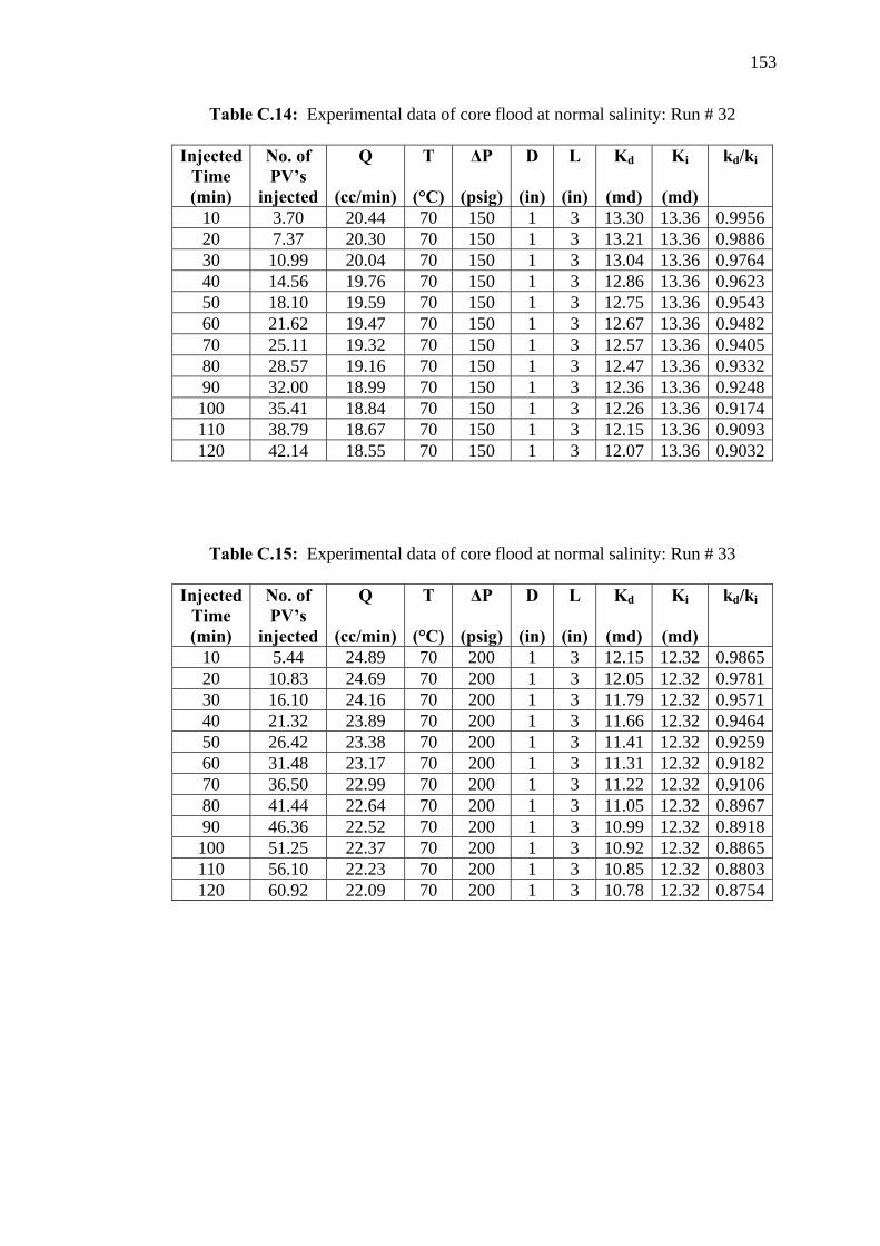
153


Injected Time (min)

No. of PV’s

injected

Q

(cc/min)

T

(°C)

∆P

(psig)

D

(in)

L

(in)

Kd

(md)

Ki

(md)

kd/ki

10 3.70 20.44 70 150 1 3 13.30 13.36 0.995620 7.37 20.30 70 150 1 3 13.21 13.36 0.988630 10.99 20.04 70 150 1 3 13.04 13.36 0.976440 14.56 19.76 70 150 1 3 12.86 13.36 0.962350 18.10 19.59 70 150 1 3 12.75 13.36 0.954360 21.62 19.47 70 150 1 3 12.67 13.36 0.948270 25.11 19.32 70 150 1 3 12.57 13.36 0.940580 28.57 19.16 70 150 1 3 12.47 13.36 0.933290 32.00 18.99 70 150 1 3 12.36 13.36 0.9248100 35.41 18.84 70 150 1 3 12.26 13.36 0.9174110 38.79 18.67 70 150 1 3 12.15 13.36 0.9093120 42.14 18.55 70 150 1 3 12.07 13.36 0.9032


Injected Time (min)

No. of PV’s

injected

Q

(cc/min)

T

(°C)

∆P

(psig)

D

(in)

L

(in)

Kd

(md)

Ki

(md)

kd/ki

10 5.44 24.89 70 200 1 3 12.15 12.32 0.986520 10.83 24.69 70 200 1 3 12.05 12.32 0.978130 16.10 24.16 70 200 1 3 11.79 12.32 0.957140 21.32 23.89 70 200 1 3 11.66 12.32 0.946450 26.42 23.38 70 200 1 3 11.41 12.32 0.925960 31.48 23.17 70 200 1 3 11.31 12.32 0.918270 36.50 22.99 70 200 1 3 11.22 12.32 0.910680 41.44 22.64 70 200 1 3 11.05 12.32 0.896790 46.36 22.52 70 200 1 3 10.99 12.32 0.8918100 51.25 22.37 70 200 1 3 10.92 12.32 0.8865110 56.10 22.23 70 200 1 3 10.85 12.32 0.8803120 60.92 22.09 70 200 1 3 10.78 12.32 0.8754

154


Injected Time (min)

No. of PV’s

injected

Q

(cc/min)

T

(°C)

∆P

(psig)

D

(in)

L

(in)

Kd

(md)

Ki

(md)

kd/ki

10 2.92 14.55 80 100 1 3 12.73 12.78 0.996120 5.80 14.37 80 100 1 3 12.57 12.78 0.983230 8.65 14.17 80 100 1 3 12.40 12.78 0.970340 11.47 14.06 80 100 1 3 12.30 12.78 0.962150 14.27 13.97 80 100 1 3 12.22 12.78 0.956560 17.06 13.87 80 100 1 3 12.14 12.78 0.949870 19.82 13.75 80 100 1 3 12.03 12.78 0.941580 22.57 13.68 80 100 1 3 11.97 12.78 0.937090 25.30 13.59 80 100 1 3 11.89 12.78 0.9302100 28.02 13.54 80 100 1 3 11.85 12.78 0.9276110 30.72 13.46 80 100 1 3 11.78 12.78 0.9215120 33.41 13.39 80 100 1 3 11.72 12.78 0.9174


Injected Time (min)


Q (cc/min)

T

(°C)

∆P (psig)

D

(in)

L (in)

Kd (md)

Ki (md)

kd/ki

10 4.26 23.87 80 150 1 3 13.34 13.48 0.989420 8.45 22.53 80 150 1 3 13.14 13.48 0.975130 12.56 22.05 80 150 1 3 12.86 13.48 0.954340 16.63 21.87 80 150 1 3 12.76 13.48 0.946950 20.65 21.57 80 150 1 3 12.58 13.48 0.933660 24.64 21.41 80 150 1 3 12.49 13.48 0.926670 28.60 21.24 80 150 1 3 12.39 13.48 0.919580 32.52 21.07 80 150 1 3 12.29 13.48 0.912090 36.42 20.95 80 150 1 3 12.22 13.48 0.9065100 40.29 20.79 80 150 1 3 12.13 13.48 0.8998110 44.14 20.66 80 150 1 3 12.05 13.48 0.8936120 47.95 20.49 80 150 1 3 11.95 13.48 0.8868

155


Injected Time (min)


Q (cc/min)

T

(°C)

∆P (psig)

D

(in)

L (in)

Kd (md)

Ki (md)

kd/ki

10 7.54 31.33 80 200 1 3 13.27 13.54 0.980320 14.99 30.94 80 200 1 3 13.10 13.54 0.967430 22.27 29.28 80 200 1 3 12.81 13.54 0.946140 29.46 28.91 80 200 1 3 12.65 13.54 0.934050 36.54 28.46 80 200 1 3 12.45 13.54 0.919360 43.50 27.98 80 200 1 3 12.24 13.54 0.904170 50.41 27.77 80 200 1 3 12.15 13.54 0.897380 57.17 27.47 80 200 1 3 12.02 13.54 0.887990 63.93 27.18 80 200 1 3 11.89 13.54 0.8781100 70.61 26.86 80 200 1 3 11.75 13.54 0.8680110 77.23 26.60 80 200 1 3 11.64 13.54 0.8596120 83.80 26.42 80 200 1 3 11.56 13.54 0.8536

156

APPENDIX D

EFFECTS OF TEMPERATURE, CONCENTRATION OF BRINE, AND

DIFFERENTIAL PRESSURES ON PERMEABILITY REDUCTION BY

DEPOSITION OF BARIUM SULFATE

5

10

15

0 20 40 60 80 100 120Time (min)

Flow

rate

(cc/

min

)

T = 50 °CT = 70 °CT = 80 °C

∆P = 100 psig Ba = 2200 ppm

5

7

9

11

13

15

17

19

21

0 20 40 60 80 100 120Time (min)

Flow

rate

(cc/

min

)

T = 50 °CT = 70 °CT = 80 °C

∆P = 150 psig Ba = 2200 ppm

10

12

14

16

18

20

22

24

26

28

0 20 40 60 80 100 120Time (min)

Flow

rate

(cc/

min

)

T = 50 °CT = 70 °CT = 80 °C

∆P = 200 psig Ba = 2200 ppm

7

8

9

10

11

12

13

14

15

0 20 40 60 80 100 120Time (min)

Flow

rate

(cc/

min

)

T = 50 °CT = 70 °CT = 80 °C

∆P = 100 psig Ba = 250 ppm

157

10

12

14

16

18

20

22

0 20 40 60 80 100 120Time (min)

Flow

rate

(cc/

min

)

T = 50 °CT = 70 °CT = 80 °C

∆P = 150 psig Ba = 250 ppm

15

17

19

21

23

25

27

29

0 20 40 60 80 100 120Time (min)

Flow

rate

(cc/

min

)

T = 50 °CT = 70 °CT = 80 °C

∆P = 200 psig Ba = 250 ppm

Figures D 1 - 6 Variation of flow rate as a function of time showing the effect of

temperature

2

6

10

14

18

22

0 20 40 60 80 100 120Time (min)

Flow

rate

(cc/

min

)


T = 50 °C Ba = 2200 ppm

4

9

14

19

24

0 20 40 60 80 100 120Time (min)

Flow

rate

(cc/

min

)


T = 70 °C Ba = 2200 ppm

5

10

15

20

25

30

0 20 40 60 80 100 120Time (min)

Flow

rate

(cc/

min

)


T = 80 °C Ba = 2200 ppm

2

6

10

14

18

22

0 20 40 60 80 100 120Time (min)

Flow

rate

(cc/

min

)


T = 50 °C Ba = 250 ppm

158

4

8

12

16

20

24

0 20 40 60 80 100 120Time (min)

Flow

rate

(cc/

min

)


T = 70 °C Ba = 250 ppm

4

8

12

16

20

24

28

0 20 40 60 80 100 120Time (min)

Flow

rate

(cc/

min

)


T = 80 °C Ba = 250 ppm

Figures D.7 – 12 Variation of flow rate as a function of time showing the effect

of differential pressure

7

8

9

10

11

12

0 20 40 60 80 100 120Time (min)

Flow

rate

(cc/

min

)

∆P = 100 psig T = 50 °C

Ba = 250 ppm

Ba = 2200 ppm

12

13

14

15

16

17

0 20 40 60 80 100 120Time (min)

Flow

rate

(cc/

min

)

∆P = 150 psig T = 50 °C

Ba = 250 ppm

Ba = 2200 ppm

17

18

19

20

21

22

0 20 40 60 80 100 120Time (min)

Flow

rate

(cc/

min

)

∆P = 200 psig T = 50 °C

Ba = 250 ppm

Ba = 2200 ppm

10

10.5

11

11.5

12

12.5

13

0 20 40 60 80 100 120Time (min)

Flow

rate

(cc/

min

)

∆P = 100 psig T = 70 °C

Ba = 250 ppm

Ba = 2200 ppm

159

15

16

17

18

19

20

21

0 20 40 60 80 100 120Time (min)

Flow

rate

(cc/

min

)

∆P = 150 psig T = 70 °C

Ba = 250 ppm

Ba = 2200 ppm

20

21

22

23

24

25

26

0 20 40 60 80 100 120Time (min)

Flow

rate

(cc/

min

)

∆P = 200 psig T = 70 °C

Ba = 250 ppm

Ba = 2200 ppm

10

11

12

13

14

15

16

0 20 40 60 80 100 120Time (min)

Flow

rate

(cc/

min

)

∆P = 100 psig T = 80 °C

Ba = 250 ppm

Ba = 2200 ppm

16

17

18

19

20

21

22

23

0 20 40 60 80 100 120Time (min)

Flow

rate

(cc/

min

)

∆P = 150 psig T = 80 °C

Ba = 250 ppm

Ba = 2200 ppm

22

23

24

25

26

27

28

29

0 20 40 60 80 100 120Time (min)

Flow

rate

(cc/

min

)

∆P = 200 psig T = 80 °C

Ba = 250 ppm

Ba = 2200 ppm

Figures D.13 - 21 Variation of flow rate as a function of time showing the effect

of concentration

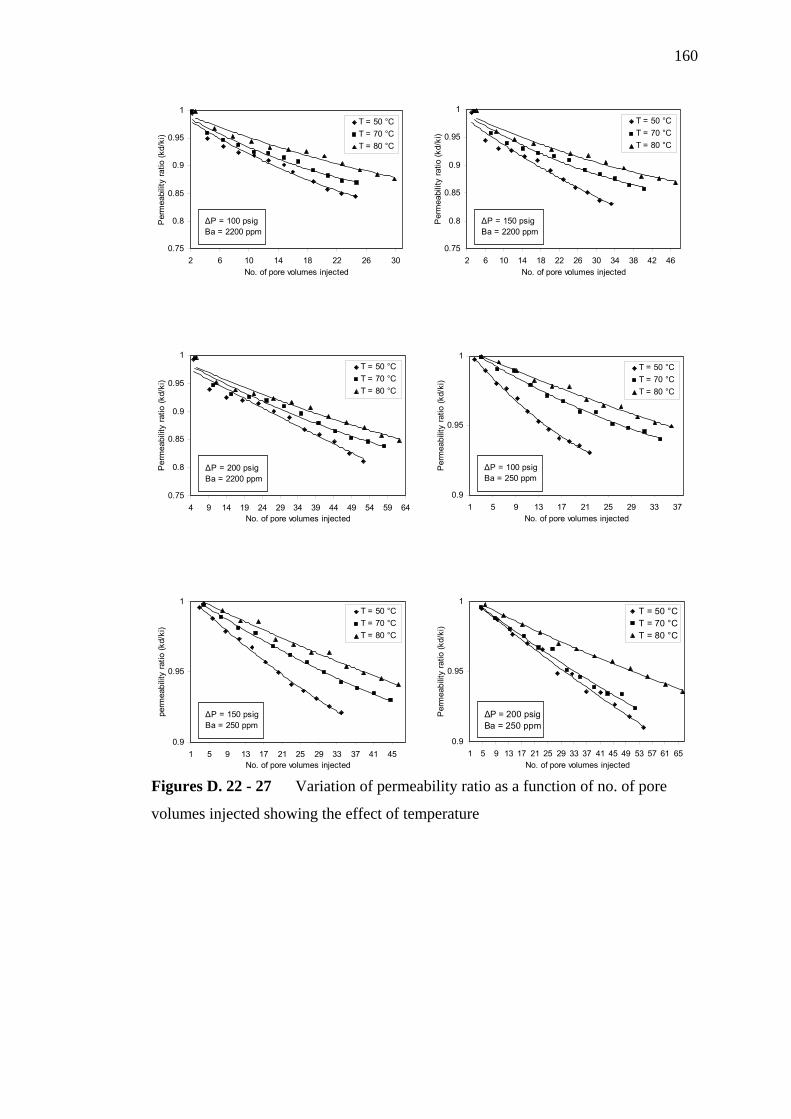
160

0.75

0.8

0.85

0.9

0.95

1

2 6 10 14 18 22 26 30No. of pore volumes injected

Per

mea

bilit

y ra

tio (k

d/ki

)

T = 50 °CT = 70 °CT = 80 °C

∆P = 100 psig Ba = 2200 ppm

0.75

0.8

0.85

0.9

0.95

1

2 6 10 14 18 22 26 30 34 38 42 46No. of pore volumes injected

Per

mea

bilit

y ra

tio (k

d/ki

)

T = 50 °CT = 70 °CT = 80 °C

∆P = 150 psig Ba = 2200 ppm

0.75

0.8

0.85

0.9

0.95

1

4 9 14 19 24 29 34 39 44 49 54 59 64No. of pore volumes injected

Per

mea

bilit

y ra

tio (k

d/ki

)

T = 50 °CT = 70 °CT = 80 °C

∆P = 200 psig Ba = 2200 ppm

0.9

0.95

1

1 5 9 13 17 21 25 29 33 37No. of pore volumes injected

Per

mea

bilit

y ra

tio (k

d/ki

)

T = 50 °CT = 70 °CT = 80 °C

∆P = 100 psig Ba = 250 ppm

0.9

0.95

1


perm

eabi

lity

ratio

(kd/

ki)

T = 50 °CT = 70 °CT = 80 °C

∆P = 150 psig Ba = 250 ppm

0.9

0.95

1

1 5 9 13 17 21 25 29 33 37 41 45 49 53 57 61 65No. of pore volumes injected

Per

mea

bilit

y ra

tio (k

d/ki

)

T = 50 °CT = 70 °CT = 80 °C

∆P = 200 psig Ba = 250 ppm

Figures D. 22 - 27 Variation of permeability ratio as a function of no. of pore

volumes injected showing the effect of temperature

161

0.75

0.8

0.85

0.9

0.95

1

2 7 12 17 22 27 32 37 42 47 52No. of pore volumes injected

Per

mea

bilit

y ra

tio (k

d/ki

)


T = 50 °C Ba = 2200 ppm

0.75

0.8

0.85

0.9

0.95

1

2 6 10 14 18 22 26 30 34 38 42 46 50 54 58No. of pore volumes injected

Per

mea

bilit

y ra

tio (k

d/ki

)


T = 70 °C Ba = 2200 ppm

0.75

0.8

0.85

0.9

0.95

1

2 6 10 14 18 22 26 30 34 38 42 46 50 54 58 62No. of pore volumes injected

Per

mea

bilit

y ra

tio (k

d/ki

)


T = 80 °C Ba = 2200 ppm

0.9

0.95

1


Per

mea

bilit

y ra

tio (k

d/ki

)


T = 50 °C Ba = 250 ppm

0.9

0.95

1


Per

mea

bilit

y ra

tio (k

d/ki

)


T = 70 °C Ba = 250 ppm

0.9

0.95

1

1 6 11 16 21 26 31 36 41 46 51 56 61 66No. of pore volumes injected

Per

mea

bilit

y ra

tio (k

d/ki

)


T = 80 °C Ba = 250 ppm

Figure D. 28 - 33 Variation of permeability ratio as a function of no. of pore

volumes injected showing the effect of differential pressure

162

0.75

0.8

0.85

0.9

0.95

1

1 5 9 13 17 21 2No. of pore volumes injected

Per

mea

bilit

y ra

tio (k

d/ki

)

5

∆P = 100 psig T = 50 °C

Ba = 250 ppm

Ba = 2200 ppm

0.75

0.8

0.85

0.9

0.95

1

1 5 9 13 17 21 25 29 33No. of pore volumes injected

Per

mea

bilit

y ra

tio (k

d/ki

)

∆P = 150 psig T = 50 °C

Ba = 250 ppm

Ba = 2200 ppm

0.75

0.8

0.85

0.9

0.95

1


Per

mea

bilit

y ra

tio (k

d/ki

)

∆P = 200 psig T = 50 °C

Ba = 250 ppm

Ba = 2200 ppm

0.75

0.8

0.85

0.9

0.95

1


Per

mea

bilit

y ra

tio (k

d/ki

)

∆P = 100 psig T = 70 °C

Ba = 250 ppm

Ba = 2200 ppm

0.75

0.8

0.85

0.9

0.95

1


Per

mea

bilit

y ra

tio (k

d/ki

)

∆P = 150 psig T = 70 °C

Ba = 250 ppm

Ba = 2200 ppm

0.75

0.8

0.85

0.9

0.95

1


Per

mea

bilit

y ra

tio (k

d/ki

)

∆P = 200 psig T = 70 °C

Ba = 250 ppm

Ba = 2200 ppm

163

0.75

0.8

0.85

0.9

0.95

1


Per

mea

bilit

y ra

tio (k

d/ki

)

∆P = 100 psig T = 80 °C

Ba = 250 ppm

Ba = 2200 ppm

0.75

0.8

0.85

0.9

0.95

1


Per

mea

bilit

y ra

tio (k

d/ki

)

∆P = 150 psig T = 80 °C

Ba = 250 ppm

Ba = 2200 ppm

0.75

0.8

0.85

0.9

0.95

1

1 5 9 13 17 21 25 29 33 37 41 45 49 53 57 61 65No. of pore volumes injected

Per

mea

bilit

y ra

tio (k

d/ki

)

∆P = 200 psig T = 80 °C

Ba = 250 ppm

Ba = 2200 ppm

0.75

0.8

0.85

0.9

0.95

1


Perm

eabi

lity

ratio

(Kd/

ki)

High barium

High salinity

∆P = 200 psig T = 50 ºC

0.75

0.8

0.85

0.9

0.95

1


Perm

eabi

lity

ratio

(Kd/

ki)

High barium

High salinity

∆P = 200 psig T = 80 ºC

Figure D. 34 - 44 Variation of permeability ratio as a function of no. of pore

volumes injected showing the effect of concentration

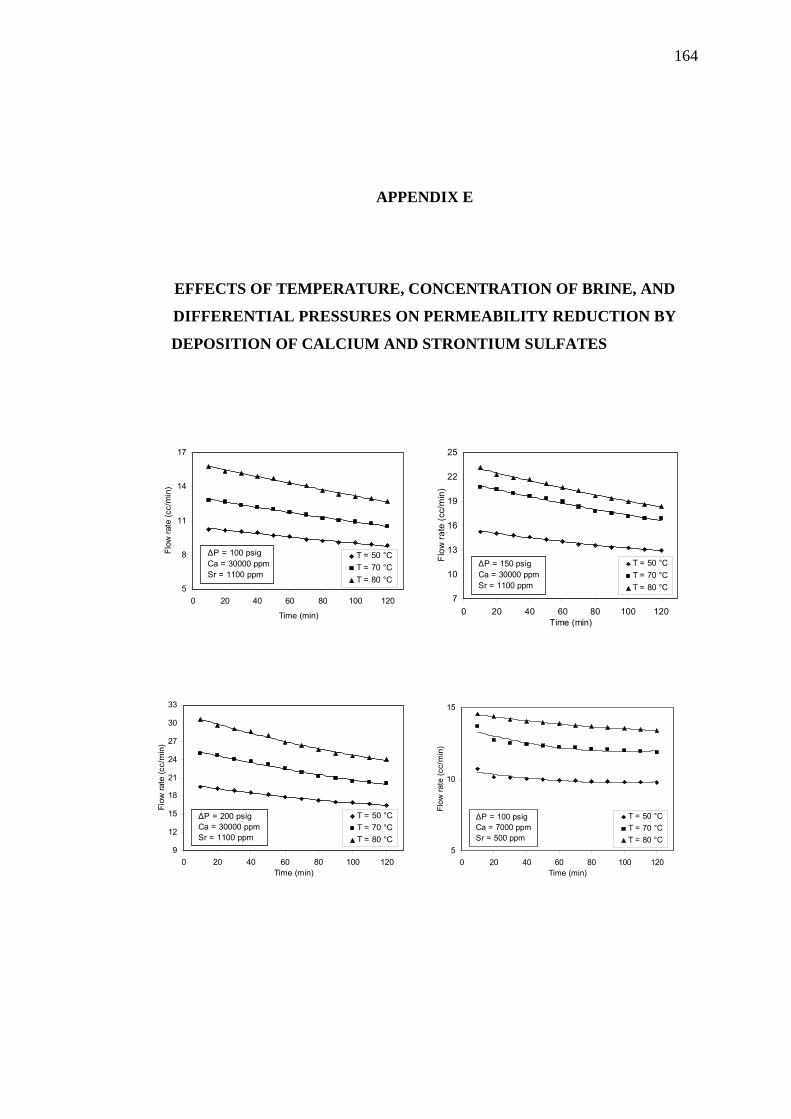
164

APPENDIX E

EFFECTS OF TEMPERATURE, CONCENTRATION OF BRINE, AND

DIFFERENTIAL PRESSURES ON PERMEABILITY REDUCTION BY

DEPOSITION OF CALCIUM AND STRONTIUM SULFATES

5

8

11

14

17

0 20 40 60 80 100 120

Time (min)

Flow

rate

(cc/

min

)

T = 50 °CT = 70 °CT = 80 °C


7

10

13

16

19

22

25

0 20 40 60 80 100 120Time (min)

Flow

rate

(cc/

min

)

T = 50 °CT = 70 °CT = 80 °C


9

12

15

18

21

24

27

30

33

0 20 40 60 80 100 120Time (min)

Flow

rate

(cc/

min

)

T = 50 °CT = 70 °CT = 80 °C


5

10

15

0 20 40 60 80 100 120Time (min)

Flow

rate

(cc/

min

)

T = 50 °CT = 70 °CT = 80 °C


165

10

14

18

22

0 20 40 60 80 100 120Time (min)

Flow

rate

(cc/

min

)

T = 50 °CT = 70 °CT = 80 °C


10

14

18

22

26

30

0 20 40 60 80 100 120Time (min)

Flow

rate

(cc/

min

)

T = 50 °CT = 70 °CT = 80 °C


Figures E. 1 - 6 Variation of flow rate as a function of time showing the effect of

temperature

2

6

10

14

18

0 20 40 60 80 100 120Time (min)

Flow

rate

(cc/

min

)


T = 50°C Ca = 30000 ppm Sr = 1100 ppm

3

8

13

18

23

0 20 40 60 80 100 120Time (min)

Flow

rate

(cc/

min

)


T = 70 °C Ca = 30000 ppm Sr = 1100 ppm

4

9

14

19

24

29

0 20 40 60 80 100 120Time (min)

Flow

rate

(cc/

min

)


T = 80 °C Ca = 30000 ppm Sr = 1100 ppm

3

7

11

15

19

0 20 40 60 80 100 120Time (min)

Flow

rate

(cc/

min

)


T = 50 °C Ca = 7000 ppm Sr = 500 ppm

166

3

7

11

15

19

23

0 20 40 60 80 100 120Time (min)

Flow

rate

(cc/

min

)


T = 70 °C Ca = 7000 ppm Sr = 500 ppm

3

7

11

15

19

23

27

31

0 20 40 60 80 100 120Time (min)

Flow

rate

(cc/

min

)


T = 80 °C Ca = 7000 ppm Sr = 500 ppm

Figures E.7 - 12 Variation of flow rate as a function of time showing the effect of

differential pressure

8

8.5

9

9.5

10

10.5

11

0 20 40 60 80 100 120Time (min)

Flow

rate

(cc/

min

)

High salinity

Normal salinity

∆P = 100 psig T = 50 °C

11

12

13

14

15

16

0 20 40 60 80 100 120Time (min)

Flow

rate

(cc/

min

)

High salinity


15

16

17

18

19

20

0 20 40 60 80 100 120Time (min)

Flow

rate

(cc/

min

)

High salinity

Normal salinity

∆P = 200 psig T = 50 °C

8

9

10

11

12

13

14

0 20 40 60 80 100 120

Time (min)

Flow

rate

(cc/

min

)

High salinity


167

15

16

17

18

19

20

21

22

0 20 40 60 80 100 120

Time (min)

Flow

rate

(cc/

min

)

High salinity

Normal salinity

∆P = 150 psig T = 70 °C

17

18

19

20

21

22

23

24

25

26

0 20 40 60 80 100 120

Time (min)

Flow

rate

(cc/

min

)

High salinity


15

16

17

18

19

20

21

22

23

0 20 40 60 80 100 120

Time (min)

Flow

rate

(cc/

min

)

High salinity


2223242526272829303132

0 20 40 60 80 100 120

Time (min)

Flow

rate

(cc/

min

)

High salinity

Normal salinity

∆P = 200 psig T = 80 °C

Figures E.13 - 20 Variation of flow rate as a function of time showing the effect

of concentration

0.75

0.8

0.85

0.9

0.95

1

1 5 9 13 17 21 25 29 33 37No. of pore volumes injected

Per

mea

bilit

y ra

tio (k

d/ki

)

T = 50 °CT = 70 °CT = 80 °C


0.75

0.8

0.85

0.9

0.95

1


Per

mea

bilit

y ra

tio (k

d/ki

)

T = 50 °CT = 70 °CT = 80 °C


168

0.75

0.8

0.85

0.9

0.95

1


Per

mea

bilit

y ra

tio (k

d/ki

)

T = 50 °CT = 70 °CT = 80 °C


0.85

0.9

0.95

1


Per

mea

bilit

y ra

tio (k

d/ki

)

T = 50 °CT = 70 °CT = 80 °C


0.85

0.9

0.95

1

1 5 9 13 17 21 25 29 33 37 41 45 49No. of Pore Volumes Injected

Per

mea

bilit

y ra

tio (k

d/ki

)

T = 50 °CT = 70 °CT = 80 °C


0.85

0.9

0.95

1


Per

mea

bilit

y ra

tio (k

d/ki

)

T = 50 °CT = 70 °CT = 80 °C


Figures E. 21 - 26 Variation of permeability ratio as a function of no. of pore

volumes injected showing the effect of temperature

0.75

0.8

0.85

0.9

0.95

1


Per

mea

bilit

y ra

tio (k

d/ki

)


T = 50 °C Ca = 30000 ppm Sr = 1100 ppm

0.75

0.8

0.85

0.9

0.95

1


Per

mea

bilit

y ra

tio (k

d/ki

)


T = 70 °C Ca = 30000 ppm Sr = 1100 ppm

169

0.75

0.8

0.85

0.9

0.95

1


Per

mea

bilit

y ra

tio (k

d/ki

)


T = 80 °C Ca = 30000 ppm Sr = 1100 ppm

0.85

0.9

0.95

1


Per

mea

bilit

y ra

tio (k

d/ki

)


T = 50 °C Ca = 7000 ppm Sr = 500 ppm

0.85

0.9

0.95

1


Per

mea

bilit

y ra

tio (k

d/ki

)


T = 70 °C Ca = 7000 ppm Sr = 500 ppm

0.85

0.9

0.95

1


Per

mea

bilit

y ra

tio (k

d/ki

)


T = 80°C Ca = 7000 ppm Sr = 500 ppm

Figure E. 27 - 32 Variation of permeability ratio as a function of no. of pore

volumes injected showing the effect of differential pressure

0.75

0.8

0.85

0.9

0.95

1

1 5 9 13 17 21No. of pore volumes injected

Per

mea

bilit

y ra

tio (k

d/ki

)

High salinity

Normal salinity

∆P = 100 psig T = 50 °C

0.75

0.8

0.85

0.9

0.95

1


Per

mea

bilit

y ra

tio (k

d/ki

)

High salinity

Normal salinity

∆P = 150 psig T = 50 °C

170

0.75

0.8

0.85

0.9

0.95

1


Per

mea

bilit

y ra

tio (k

d/ki

)

High salinity

Normal salinity

∆P = 200 psig T = 50 °C

0.75

0.8

0.85

0.9

0.95

1


Per

mea

bilit

y ra

tio (k

d/ki

)

High salinity

Normal salinity

∆P = 100 psig T = 70 °C

0.75

0.8

0.85

0.9

0.95

1

1 5 9 13 17 21 25 29 33 37 41No. of pore volumes injected

Per

mea

bilit

y ra

tio (k

d/ki

)

High salinity

Normal salinity

∆P = 150 psig T = 70 °C

0.75

0.8

0.85

0.9

0.95

1

1 5 9 13 17 21 25 29 33 37 41 45 49 53 57 61No. of pore volumes injected

Per

mea

bilit

y ra

tio (k

d/ki

)

High salinity

Normal salinity

∆P = 200 psig T = 70 °C

0.75

0.8

0.85

0.9

0.95

1


Per

mea

bilit

y ra

tio (k

d/ki

)

High salinity

Normal salinity

∆P = 100 psig T = 80 °C

0.75

0.8

0.85

0.9

0.95

1


Per

mea

bilit

y ra

tio (k

d/ki

)

High salinity

Normal salinity

∆P = 150 psig T = 80 °C

171

0.75

0.8

0.85

0.9

0.95

1

1 6 11 16 21 26 31 36 41 46 51 56 61 66 71 76 81No. of pore volumes Injected

Per

mea

bilit

y ra

tio (k

d/ki

)

High salinity

Normal salinity

∆P = 200 psig T = 80 °C

Figure E. 33 - 41 Variation of permeability ratio as a function of no. of pore

volumes injected showing the effect of concentration

the study of scale formation in oil reservoir …eprints.utm.my/id/eprint/5802/1/75224.pdf ·...

Documents