the temperature–humidity covariance in the marine surface … · institute of atmospheric...

Boundary-Layer Meteorol (2008) 126:263–278DOI 10.1007/s10546-007-9236-z

ORIGINAL PAPER

The Temperature–Humidity Covariance in the MarineSurface Layer: A One-dimensional Analytical Model

Gabriel G. Katul · Anna M. Sempreviva ·Daniela Cava

Received: 25 May 2007 / Accepted: 4 October 2007 / Published online: 26 October 2007© Springer Science+Business Media B.V. 2007

Abstract An analytical model that predicts how much of the temperature–humidity covari-ance within the marine atmospheric surface layer (ASL) originates just above the ASL andjust near the surface is proposed and tested using observations from the Risø Air Sea Experi-ment (RASEX). The model is based on a simplified budget for the two-scalar covariance thatretains three basic terms: production, dissipation, and vertical transport. Standard second-order closure formulations are employed for the triple moments and the dissipation terms,and the canonical mixing length for the closure model is assumed linear with height (z) fromthe surface. Despite the poor performance of the gradient–diffusion closure in reproduc-ing the measured triple moment, the overall covariance model was shown to be sufficientlyrobust to these assumptions. One of the main findings from the analytical treatment is theorigin of the asymmetry in how the top and bottom boundary conditions affect the two-scalarcovariance in the ASL. The analytical model reveals that ‘bottom-up’ boundary-conditionvariations scale with z−√

a , while ‘top-down’ variations scale with z√

a , where a is a constantthat can be derived from similarity and closure constants. The genesis of this asymmetry

G. G. Katul (B)Nicholas School of the Environment and Earth Sciences, Duke University, Box 90328, Durham, NC,27708-0328, USAe-mail: [email protected]

G. G. KatulDepartment of Civil and Environmental Engineering, Duke University, Durham, NC, 27708-0328, USA

A. M. SemprevivaDepartment of Wind Energy, Risø National Laboratory, Technical University of Denmark, 4000 Roskilde,Denmarke-mail: [email protected]

A. M. SemprevivaInstitute of Atmospheric Sciences and Climate, ISAC-CNR, Area di Ricerca CNR, Roma Tor Vergata,Via Fosso del Cavaliere 10, 00133 Rome, Italye-mail: [email protected]

D. CavaCNR – Institute of Atmosphere Sciences and Climate Section of Lecce, Lecces, Italye-mail: [email protected]

123

264 G. G. Katul et al.

stems from the flux-transport term but is modulated by the dissipation, and persists even inthe absence of any inhomogeneity in the local production function. It is shown that the localproduction function acts to adjust the relative proportions of these two boundary conditionswith weights that vary with the Obukhov length. The findings here do not provide ‘finality’to the discussions on the covariance between humidity and temperature or the role of entrain-ment in modulating the turbulence within the ASL. Rather, they are intended to guide newhypotheses about interpretations of existing field data and identify needs for future field andnumerical experiments.

Keywords Atmospheric surface layer · Cauchy–Euler equation · Gradient–diffusionclosure · Marine surface layer · Risø Air Sea experiment · Temperature–humidity covariance

1 Introduction

Over the last three decades, the temperature (T )–humidity (C) covariance (T ′C ′) in theatmospheric surface layer (ASL) has received significant attention, partly because of its usein assessing similarities in bulk scalar transfer parameters (e.g., Hill 1989), electromagneticwave propagation in a non-ionized atmosphere (Friehe et al. 1975; Wesley 1976), amongothers. Here, primed quantities are turbulent excursions from time-averaged variables, andthe overbar indicates a time-averaged quantity. While these issues all deserve attention,examining the main mechanisms by which the covariance between two scalar fluctuationsis produced, maintained, or dissipated is a legitimate fundamental problem in its own right.Understanding these mechanisms can highlight new dynamical processes modulating thestructure of turbulence within the ASL not readily detected by other approaches. In fact, theymay even provide blue prints on how to proceed on other practical yet unresolved issuessuch as the imbalance between available net radiation and the sum of sensible and latent heatfluxes (e.g., Steinfeld et al. 2007).

A number of studies listed in Table 1 have suggested that dissimilarities in the temper-ature–humidity covariance is often attributed to one (or more) of the following causes: (i)the active roles of temperature (and humidity) in the production/destruction of turbulentkinetic energy, (ii) advection of heat or moisture (both longitudinally and vertically), (iii)unsteadiness in the outer-layer flow that can impinge on the ASL, (iv) source inhomogeneityat the ground surface, and (v) local entrainment processes from the top of the atmosphericboundary layer (ABL). In the upper part of the ABL, the correlation coefficient betweenheat and water vapour (RT C ) is generally negative because of the entrainment of warm yetdry air. Hence, it is conceivable that any observed reductions from unity in RT C within theASL can be partially explained by this top-down mixing of drier air (see Table 1 for refer-ences). Though this latter argument is intuitive and theoretically appealing, the large distanceseparating the ASL from the entrainment zone, and the ubiquitous presence of other ‘con-taminating’ issues (e.g., averaging times and non-stationarity as in Asanuma et al. 2007),make this entrainment argument difficult to establish (see e.g., Andreas et al. 1998; De Bruinet al. 1999).

Progress on the latter point can benefit from an explicit expression that describes how ananti-correlation between temperature and humidity at some level within the ABL propagatesdown into the ASL. In particular, we seek a simplified expression that predicts how much ofthe dissimilarity in the temperature–humidity covariance within the ASL originates from aboundary condition above the ASL or from source dissimilarities at the ground, the subjectof this study.

123

Temperature–Humidity Covariance in the Marine Surface Layer 265

Table 1 Sample studies that reported or discussed covariances and cospectra between temperature and watervapour concentration and possible reasons why their correlation diverges from unity within the atmosphericsurface layer

Active roles of temperature (and water vapour)

Flux–gradient (or Roughness) similarity functions: Warhaft (1976), Papaioannou et al. (1989), King andAnderson (1994), Dias and Brutsaert (1996)

Flux–variance similarity functions: Katul and Hsieh (1999)General turbulence: See Katul and Parlange (1994), Nagata and Komori (2001) for detailed references on

active/passive scalars

Advective conditions

Vegetation: Verma et al. (1978), Lang et al. (1983), Wesley (1988), Kroon and De Bruin (1995),McNaughton and Laubach (2000)

Lakes and reservoirs: Assouline et al. (2007)

Modulations from the outer layer (and unsteadiness)

McNaughton and Laubach (1998), McNaughton and Brunet (2002), Högström (1990), Högström et al.(2002), Cullen et al. (2007). The recent analysis in Asanuma et al. (2007) is suggestive that much of thedissimilarity originates at very low frequency (few hours) and can also be interpreted as a result ofunsteadiness. Likewise with Phelps and Pond (1971), who attributed this unsteadiness to radiativeloading. See also Table in De Bruin et al. (1999) for further discussion

Dissimilarity in ground sources and sinks

Vegetation: Weaver (1990), Padro (1993) who contrasted vegetated surfaces with wetlands; Liu et al.(1998), Kustas et al. (1994), Katul et al. (1995, 1996), Andreas et al. (1998), Asanuma and Brutsaert(1999), Choi et al. (2004), Lamaud and Irvine (2006) demonstrated that the dissimilarity is dependent onthe surface Bowen ratio; Williams et al. (2007) demonstrated that the dissimilarity is dependent on leafarea dynamics. The latter two studies do not exclude the possibility of other factors

Urban: Moriwaki and Kanda (2006)

Entrainment processes

LES of a convective boundary layer: Moeng and Wyngaard (1984), Piper et al. (1995)Vegetation: Mahrt (1991), Mahrt et al. (2001b), De Bruin et al. (1991), De Bruin et al. (1999), Asanuma et

al. (2007)Urban: Roth and Oke (1995), Moriwaki and Kanda (2006)Marine: Wyngaard et al. (1978), Coulman (1980), Sempreviva and Gryning (2000)

Some studies report more than a singular cause

Using a simplified one-dimensional budget model forT ′C ′ that retains production, dis-sipation, and vertical transport, an analytical solution is proposed that predicts the verticalprofile of T ′C ′ from specified boundary conditions just above the ASL and at the groundsurface. There are numerous processes that contribute to the T ′C ′ budget not considered here,such as non-stationarity, mean advection, and longitudinal turbulent transport processes, andexamining all of them simultaneously is well beyond the scope of a single study. Neverthe-less, even in the presence of all these extra processes, the three terms selected here must beretained in the general budget of T ′C ′.

The marine surface layer is ideal for analyzing such a model because temperature–humid-ity similarity often exists at (or near) the surface, and advective conditions can be mini-mized by a suitable choice of wind directions. The lower ‘boundary condition’ imposedon the T ′C ′ budget is less difficult to describe over an extensive water surface, at leastwhen compared to their vegetated or urban canopy surface counterparts. Near vegetatedsurfaces, T ′C ′ is influenced by complex biological processes, while near urban settings itis influenced by patchy water vapour and heat source distributions that are not spatiallyco-located.

123


Observations from RASEX (Risø Air Sea EXperiment), collected at an offshore site inDenmark during a campaign in the Autumn of 1994 (Højstrup et al. 1995; Mahrt et al. 1998,2001a) are used here as a case study. This dataset has the added benefit in that the localproduction term of the T ′C ′ budget has been studied and shown to scale with surface-layersimilarity theory (Sempreviva and Højstrup 1998).

2 The RASEX Experiment

Often labelled as the ‘Kansas of the sea’, the RASEX set-up has been described in a numberof studies (Højstrup et al. 1995; Sempreviva and Højstrup 1998; Mahrt et al. 1998, 2001a)and only salient features are repeated here for completeness. Data used were collected ata 48-m tower situated offshore in about 4-m water depth but with upstream water depthsvarying from 5 to 20-m. Two OPHIR hygrometers, mounted at 18 and 32-m, were used formeasuring moisture fluctuations, and two Gill Solent sonic anemometers, co-located withthe OPHIR instruments, were also used to provide velocity statistics, scalar fluxes, and triplecorrelations. Data were sampled at 20 Hz and 30-min average statistics were then computed,whilst temperature data from the sonic anemometer were corrected for (1) cross wind speedfluctuations along the skewed sonic path (Schotanus et al. 1983; Kaimal and Gaynor 1991),and (2) transducer shadow effect. The analyses were restricted to winds originating from thesector 230◦–360◦ and 000◦–045◦ ensuring the longest sea fetches.

3 Theory

The T ′C ′ budget for a stationary and planar homogeneous flow, in the absence of subsidence,reduces to (e.g., Stull 1988; Garratt 1992; Sempreviva and Højstrup 1998; Juang et al. 2006)

∂T ′C ′∂t

= 0 = −(

w′C ′ ∂T

∂z+ w′T ′ ∂C

∂z

)− 2εT C − ∂w′T ′C ′

∂z, (1)

where T and C are instantaneous air temperature and water vapour concentration, respec-tively, w is the instantaneous vertical velocity, z is the height above the surface, t is time,and as before, primed quantities are turbulent excursions around their time-averaged statesindicated by the overbar. The first term on the right-hand side of Eq. 1 is the productionresponsible for locally generating the covariance between temperature and humidity; thesecond is the dissipation rate responsible for the de-correlation between these two scalars,and the third is the flux-transport term responsible for non-local transport of T ′C ′ from otherregions in the flow domain.

Using a standard closure model (e.g., Donaldson 1973; Juang et al. 2006) for the dissipa-tion, given by

εT C = Q

λ3T ′C ′, (2)

and for the flux-transport term, given by

w′T ′C ′ = −Qλ1∂T ′C ′

∂z, (3)

123


Equation 1 reduces to

λ1 Q∂2

(T ′C ′

)∂z∂z

+ ∂ (λ1 Q)

∂z

∂T ′C ′∂z

− 2

λ3QT ′C ′ =

(w′C ′ ∂T

∂z+ w′T ′ ∂C

∂z

), (4)

where Q =(

u′2 + v′2 + w′2)1/2

is a characteristic turbulent velocity scale, u and v are

the longitudinal and lateral velocity components, respectively, defined such that v̄ = 0,λ1 = A1(lm) and λ3 = A3 (lm) are related to the canonical mixing length lm , and A1and A3

are similarity constants to be determined later.

3.1 Simplifications and Analytical Treatment

For analytical tractability, Eq. 4 must be further simplified. In the ASL, these simplificationsinclude:(i) The use of a linear lm(= kv z), where kv is Von Karman’s constant.(ii) The argument that the local production term in Eq. 4 does not diverge appreciably fromsurface-layer similarity scaling. Noting that w′C ′ = u∗C∗, w′T ′ = u∗T∗, the mean scalargradients in the production term are estimated via similarity theory:

∂T

∂z

(kvz

−T∗

)= φT

( z

L

), (5a)

∂C

∂z

(kvz

−C∗

)= φC

( z

L

), (5b)

where L is the Obukhov length, and φT and φc are the standard mean gradient stabilitycorrection functions.Hence, with this simplification to the mean scalar gradients, Eq. 4 becomes:

λ1 Q∂2

(T ′C ′

)∂z∂z

+ ∂ (λ1 Q)

∂z

∂T ′C ′∂z

− 2

λ3QT ′C ′ = −u∗C∗T∗

kvz(φT (z/L) + φc(z/L))

≈ −2u∗C∗T∗

kvzφT (z/L). (6)

Again, it should be emphasized thatφT (z/L) �= φc(z/L)for a number of reasons (see Table 1).However, these differences are (a) likely to be smaller than errors introduced by the closuremodel for the flux-transport or dissipation terms, (b) less significant when compared to theoverall vertical variations in T ′C ′. For reference, it suffices to note that T ′C ′/T∗C∗ can varyfrom −20 to 20 within the convective ABL (Wyngaard et al. 1978). Again, if the differencesbetween φT (z/L) and φc(z/L) are known or even vary with T ′C ′, they can be accountedfor, though analytical tractability may become difficult for the latter case.(iii) The term

∂ (λ1 Q)

∂z

∂T ′C ′∂z

=(

Q∂ (λ1)

∂z+ λ1

∂ Q

∂z

)∂T ′C ′

∂z≈ A1kv Q

∂T ′C ′∂z

.

This argument is accurate for a near-neutral ASL, but as pure convective conditions areapproached, both terms can become significant. As we show later, this assumption is not toorestrictive for modelling T ′C ′/T∗C∗ in the lower layers of the ASL.

123


With these three simplifications, Eq. 6 reduces to:

A1kvzQ∂2T ′C ′∂z∂z

+ A1kv Q∂T ′C ′

∂z− 2

A3kvzQT ′C ′ = −2C∗T∗u∗

φT (z/L)

kvz, (7)

and upon multiplying by z and dividing by A1kv Q, this reduces to:

z2 ∂2T ′C ′∂z∂z

+ z∂T ′C ′

∂z− 2

A3 A1k2v

T ′C ′ = −2C∗T∗(

u∗Q

)φT (z/L)

A1k2v

. (8)

Noting that Q/u∗ = √2φT K E , where φT K E is the stability correction function for the

turbulent kinetic energy (TKE), Eq. 8 can now be expressed in dimensionless form as:

z2 ∂2(T ′C ′/C∗T∗)∂z∂z

+ z∂(T ′C ′/C∗T∗)

∂z−

(2

A3 A1k2v

)T ′C ′C∗T∗

= −(

2

A1k2v

)φT√

2φT K E. (9)

In Eq. 9, when ∂w′T ′C ′∂z = 0, or production balances the dissipation rate, the covariance

budget equation becomes

T ′C ′C∗T∗

= A3φT√

2 φT K E, (10)

and scales with z/L if φT K E only scales with z/L or both z/L and zi/L (where zi is theboundary-layer height), as discussed in Hsieh and Katul (1997).

3.2 Homogeneous and General Solutions

Equation 9 is a non-homogeneous Cauchy–Euler equation of the form

z2 d2 y

dz2 + zdy

dz− ay = r(z), (11)

where y = T ′C ′T∗C∗ , a = 2

A3 A1k2v

> 0, and r(z) = −(

2A1k2

v

)φT√

2φT K E, and whose homogeneous

solution (i.e., when r(z) = 0, or physically when the T ′C ′ budget is expressed without thelocal production term) is given by

yh(z) = B1z√

a + B2z−√a . (12)

When z → 0, the homogeneous solution is governed by yh(z) → B2z−√a , and when

z → +∞, yh(z) → B1z√

a . In short, these two homogeneous solutions can be interpreted asindicators of how variations in the upper and lower boundary conditions affect the normal-ized T ′C ′ values at a given height in the ASL. Physically, if a boundary condition injects afinite T ′C ′ (whether from the top or the bottom of the flow domain), the homogeneous solu-tion describes the interplay between its transport away from the boundary and its eventualdissipation in the absence of local production.

To account for this local production, a particular adjustment to yh is necessary. To derivethis particular adjustment, we note that the Wronskian (= Wr(y1, y2)) of these two homoge-neous solutions (i.e., y1 = z

√a , y2 = z−√

a) is

Wr(y1, y2) =∣∣∣∣ y1 y2

dy1dz

dy2dz

∣∣∣∣=

∣∣∣∣∣ z√

a z−√a

√az

√a−1 −√

az−√a−1

∣∣∣∣∣ = −√az−1 − √

az−1 = −2√

a

z�= 0. (13)

123


A finite Wronskian is suggestive that the ‘Method of Variation of Parameters’ can be used toinfer this particular solution (yp) and correct for r(z) �= 0. The general solution can then beexpressed as

y(z) = yh(z) + yp(z), (14)

where yp = f1(z)z√

a + f2(z)z−√a , f1 = − ∫ z−√

ar(z)Wr(z) dz, f2 = ∫ z

√ar(z)

Wr(z) dz.Hence, the final solution is given by

T ′C ′T∗C∗

=[

B1 + 1

2√

a

∫z1−√

ar (z) dz

]z√

a +[

B2 − 1

2√

a

∫z1+√

ar (z) dz

]z−√

a,

(15a)

≡ B3 (L) z√

a + B4 (L) z−√a (15b)

where

B3(L) = B1 +( −1

A1 k2v

)1√2

A3 A1 k2v

∫ ⎛⎝z

1−√

2A3 A1 k2

vφT (z/L)√

2 φT K E (z/L)

⎞⎠ dz, (16a)

B4(L) = B2 +(

1

A1 k2v

)1√

2A3 A1 k2

v

∫ ⎛⎝z

1+√

2A3 A1 k2

vφT (z/L)√

2 φT K E (z/L)

⎞⎠ dz. (16b)

Note in Eq. 16 that, because the integration is carried out over z, B3 and B4 vary only withL once the closure constants are specified. The values of B1 and B2 must be evaluated fromthe boundary conditions specified near the ground and near the top of the ASL. Equation 15still maintains that the impact of the two boundary conditions is asymmetric—the influenceof the upper boundary condition tends to scale as z

√a and its contribution diminishes as the

surface is approached, while the influence of the lower boundary condition tends to scale asz−√

a , and its influence rapidly diminishes with increasing z. The integrals in Eq. 15, whosegenesis are local production terms that primarily vary with L (though the height of the ABLcan be accounted for in r(z) via φT K E ), and that can be evaluated analytically. However,their general expression leads to hyper-geometric functions (expressed as series expansion)that are neither explicit nor intuitive in demonstrating how L modifies B3 or B4.

Hence, for practical calculations, numerical integration of Eq. 9 is actually as convenientas a numerical integration of B3 and B4, and hereafter, we refer to this numerical solutionas the model solution. Again, the main advantage of the analytical expression here is notcomputational but is intended to discern how the influences of the upper and lower boundaryconditions propagate with z within the ASL.

4 Results

To address the study objectives, it is necessary to (i) estimate the two similarity constantsA1 and A3, (ii) explore how well the gradient–diffusion closure assumption reproduces thetriple moments, and (iii) evaluate the overall performance of the analytical model within theASL and its robustness to various simplifications.

123


4.1 Determination of the Similarity Constants

For matching the ASL diffusivity under ideal conditions, λ1 Q = (A1kvz)Q = kvzu∗, andhence

A1 = 1√12

(A2

u + A2v + A2

w

) , (17)

where, for near-neutral conditions, Au = σu/u∗ ≈ 2.7, Av = σv/u∗ ≈ 2.1, and Aw =σw/u∗ ≈ 1.25 resulting in an estimated A1 ≈ 0.39.

To determine A3, recall that when ∂w′T ′C ′∂z = 0

T ′C ′C∗T∗

= A3φT√

2φT K E, (17a)

and

T ′C ′C∗ T∗

1σTT∗

σcC∗

= RT C = A3

(φT√

2φT K E

)1

φT T φcc. (17b)

Here, σs =(

s′s′)1/2

is the standard deviation of an arbitrary flow variable s, and σT /T∗ =φT T and σc/C∗ = φcc are the scalar variance stability correction functions. A maximumA3 ≈ 5.3 ensures |RT C | ≤ 1 (see Fig. 1) when using standard surface-layer similarity theoryfunctions for φT and φT K E (formulations are presented in Hsieh and Katul 1997 and are notrepeated here), and for φT T and φcc (formulations are presented in Sorbjan 1989, Table 4.2after Tillman 1972). It should be emphasized that A3 = 5.3 is dependent on the choice ofφT , φT K E , φT T and φcc, and cannot be treated as a ‘universal’ closure constant.

4.2 The Effects of Atmospheric Stability on T ′C ′ and its Budget

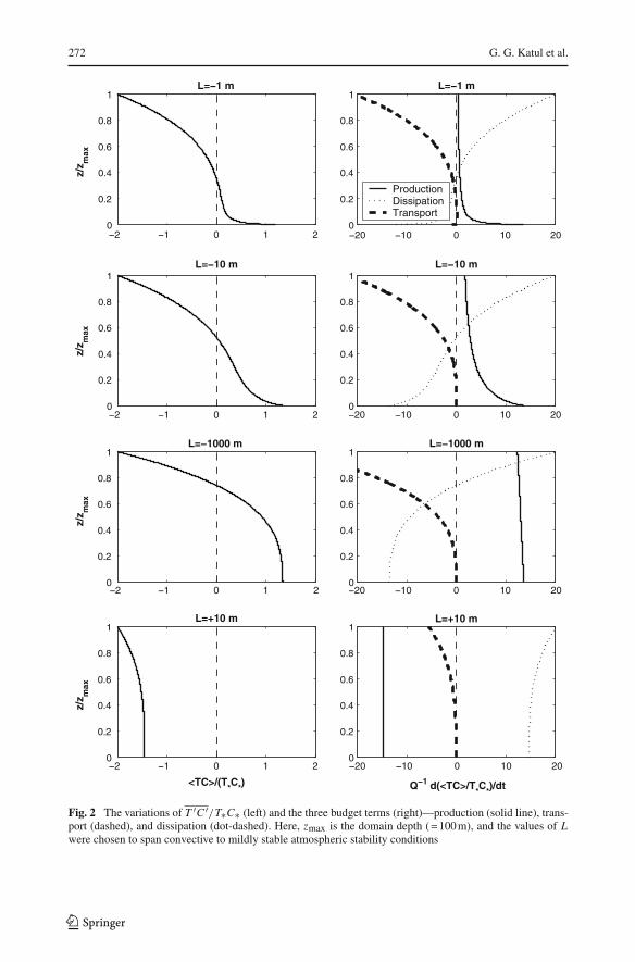
Using these two similarity constants, Fig. 2 illustrates how the upper boundary condition,fixed here at T ′C ′/(T∗C∗) = −2, affects the vertical distribution of T ′C ′/(T∗C∗) assuming∂T ′C ′/∂z = 0 at z = 0 as L varies. These model calculations were conducted by assumingthe maximum ASL height zmax = 100 m (i.e., some 10% of the mixed-layer height), and thevalue T ′C ′/(T∗C∗) = −2 was set at 10% of the maximum value near the top of the mixedlayer (e.g. Wyngaard et al. 1978), and purposely chosen as negative to initiate a dissimilaritybetween heat and water vapour at zmax. In reality, data from Wyngaard et al. (1978) suggestthat T ′C ′/(T∗C∗) = −2 occurs around the middle of the convective boundary layer (depthhcbl ) or at z = 0.5hcbl . The top of the ASL is usually around 10–20% of hcbl .

It is clear that, for near-convective conditions, this boundary condition propagates ‘deeper’into the domain when compared to the near-neutral atmospheric stability state. This propaga-tion is perhaps most evident by the height at which T ′C ′ crosses the zero value and reversessign. For near convective conditions, the ‘zero crossing’ occurs closer to the ground, whilefor near-neutral conditions, the zero crossing occurs almost mid-way in the domain. Notethat the production function of T ′C ′, also shown in Fig. 2, suggests that for near-neutralatmospheric conditions, its decay is much slower with increasing z when compared to itsconvective counterpart. Figure 2 shows that near the surface (z/zmax < 0.2), the T ′C ′ budgetis mainly governed by a balance between production and dissipation as expected, but nearthe top of the domain (around 100 m), the flux-transport term becomes significant.

123


−10 −8 −6 −4 −2 0 2−1

−0.5

0

0.5

1z=32 m

RC

T(/>

CT<=

σ Tσ C

)

−10 −8 −6 −4 −2 0 2−1

−0.5

0

0.5

1z=18 m

z/L

RC

T(/>

CT<=

σ Tσ C

)

Fig. 1 The variation of the correlation coefficient between temperature and water vapour (RT C ) with thestability parameter (z/L). Measured RT C in open circles at z = 32 m (top) and z = 18 m (bottom) fromthe RASEX are shown. The solid line reflects a balance between production and dissipation resulting in

RT C = A3

(φT√

2φT K E

)1

φT T φccwith A3 = 5.3

4.3 Gradient–Diffusion Closure Assumption

Because of the availability T ′C ′ and w′C ′T ′ at two levels, the closure assumption for thetriple moment, given by

w′T ′C ′ = −A1kvzQ∂T ′C ′

∂z(18)

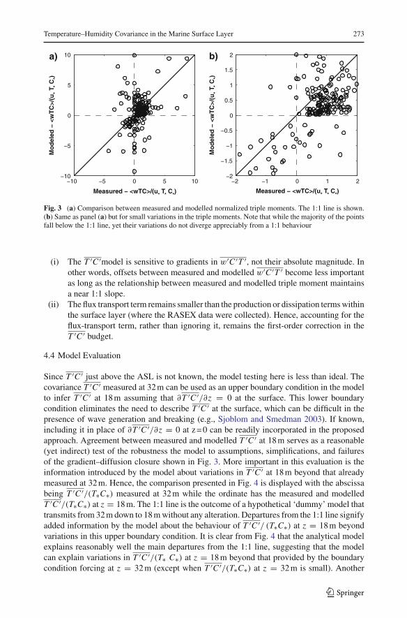
can be directly evaluated. Figure 3 shows the comparison between measured and modelledw′C ′T ′. Here, measured w′C ′T ′ as well as measured Q were computed by averaging thevalues at the two levels for each run (thus, z = 25 m is set in the diffusivity calculation), whilethe gradient in T ′C ′ was computed by differencing the measured values at the two levels.The comparison in Fig. 3 suggests that such an approximation has some predictive skills,but leaves much to be desired in the performance of a general closure model. In particular,for small magnitudes of w′C ′T ′, the gradient–diffusion approximation fails to predict thesign of the triple moment. This failure may be due to a number of factors, including mea-surement errors of the differences in T ′C ′ (as well as the finite difference approximation of∂T ′C ′/∂z), sampling errors, and instrumentation errors (including instrument separation).Whether this failure significantly degrades the model performance is explored next. How-ever, before exploring this point, we note that the modelled T ′C ′ is likely to be more robustto these issues than the modelled w′C ′T ′ for two reasons:

123


−2 −1 0 1 20

0.2

0.4

0.6

0.8

1

z/zxa

mL=−1 m

−20 −10 0 10 200

0.2

0.4

0.6

0.8

1L=−1 m

ProductionDissipationTransport

−2 −1 0 1 20

0.2

0.4

0.6

0.8

1

z/zxa

m

L=−10 m

−20 −10 0 10 200

0.2

0.4

0.6

0.8

1L=−10 m

−2 −1 0 1 20

0.2

0.4

0.6

0.8

1

z/zxa

m

L=−1000 m

−20 −10 0 10 200

0.2

0.4

0.6

0.8

1L=−1000 m

−2 −1 0 1 20

0.2

0.4

0.6

0.8

1

z/zxa

m

<TC>/(T*C

*)

L=+10 m

−20 −10 0 10 200

0.2

0.4

0.6

0.8

1

Q−1 d(<TC>/T*C

*)/dt

L=+10 m

Fig. 2 The variations of T ′C ′/T∗C∗ (left) and the three budget terms (right)—production (solid line), trans-port (dashed), and dissipation (dot-dashed). Here, zmax is the domain depth ( = 100 m), and the values of Lwere chosen to span convective to mildly stable atmospheric stability conditions

123


−10 −5 0 5 10−10

−5

0

5

10

Measured − <wTC>/(u* T

* C

*)

u(/>C

Tw< −

deled

oM

*T

*C

*)

−2 −1 0 1 2−2

−1.5

−1

−0.5

0

0.5

1

1.5

2

Measured − <wTC>/(u* T

* C

*)

u(/>C

Tw< −

deled

oM

*T

*C

*)

a) b)

Fig. 3 (a) Comparison between measured and modelled normalized triple moments. The 1:1 line is shown.(b) Same as panel (a) but for small variations in the triple moments. Note that while the majority of the pointsfall below the 1:1 line, yet their variations do not diverge appreciably from a 1:1 behaviour

(i) The T ′C ′model is sensitive to gradients in w′C ′T ′, not their absolute magnitude. Inother words, offsets between measured and modelled w′C ′T ′ become less importantas long as the relationship between measured and modelled triple moment maintainsa near 1:1 slope.

(ii) The flux transport term remains smaller than the production or dissipation terms withinthe surface layer (where the RASEX data were collected). Hence, accounting for theflux-transport term, rather than ignoring it, remains the first-order correction in theT ′C ′ budget.

4.4 Model Evaluation

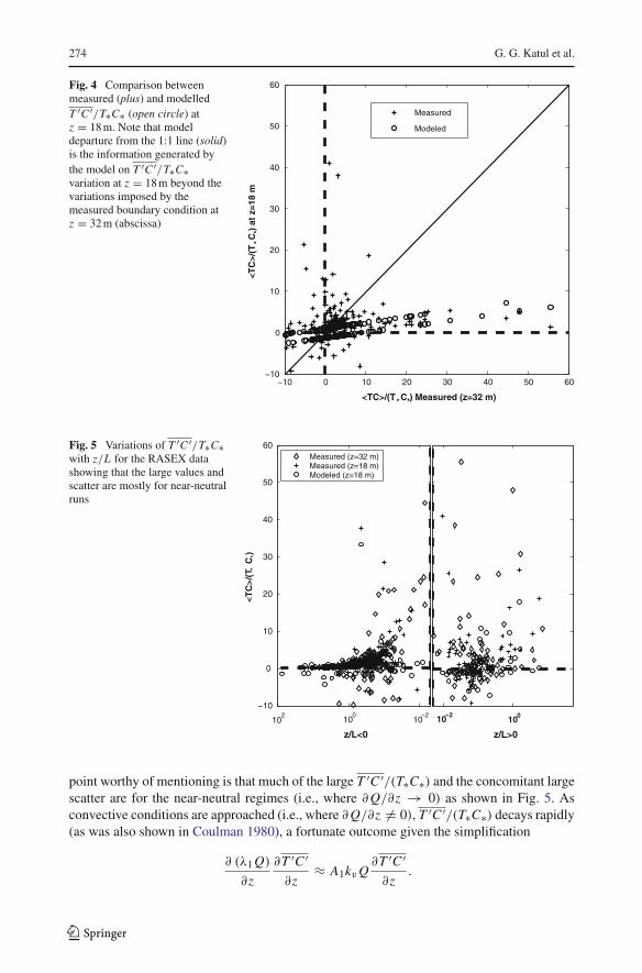
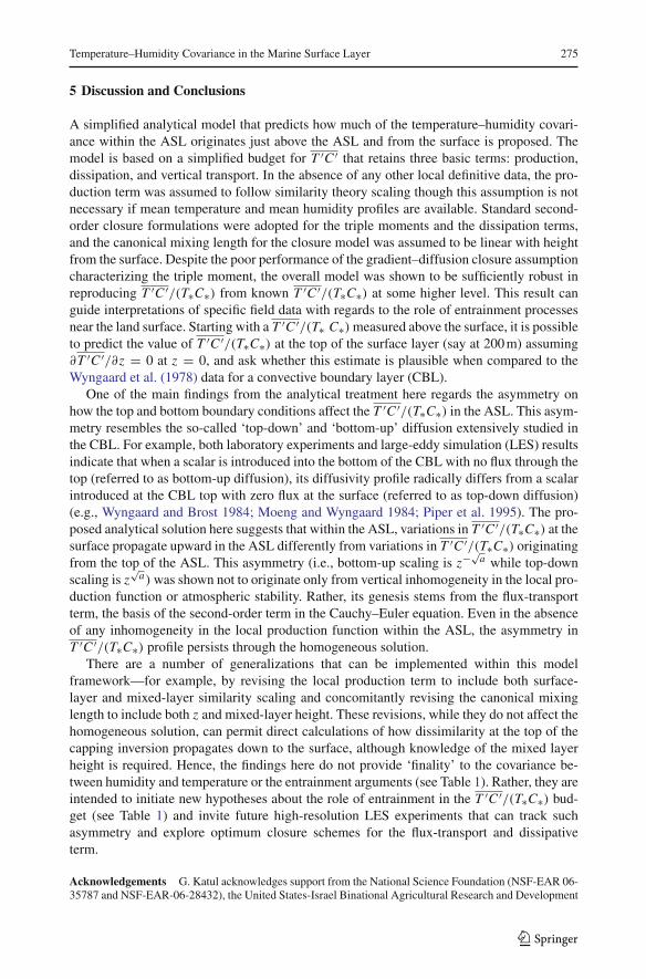
Since T ′C ′ just above the ASL is not known, the model testing here is less than ideal. Thecovariance T ′C ′ measured at 32 m can be used as an upper boundary condition in the modelto infer T ′C ′ at 18 m assuming that ∂T ′C ′/∂z = 0 at the surface. This lower boundarycondition eliminates the need to describe T ′C ′ at the surface, which can be difficult in thepresence of wave generation and breaking (e.g., Sjoblom and Smedman 2003). If known,including it in place of ∂T ′C ′/∂z = 0 at z = 0 can be readily incorporated in the proposedapproach. Agreement between measured and modelled T ′C ′ at 18 m serves as a reasonable(yet indirect) test of the robustness the model to assumptions, simplifications, and failuresof the gradient–diffusion closure shown in Fig. 3. More important in this evaluation is theinformation introduced by the model about variations in T ′C ′ at 18 m beyond that alreadymeasured at 32 m. Hence, the comparison presented in Fig. 4 is displayed with the abscissabeing T ′C ′/(T∗C∗) measured at 32 m while the ordinate has the measured and modelledT ′C ′/(T∗C∗) at z = 18 m. The 1:1 line is the outcome of a hypothetical ‘dummy’ model thattransmits from 32 m down to 18 m without any alteration. Departures from the 1:1 line signifyadded information by the model about the behaviour of T ′C ′/ (T∗C∗) at z = 18 m beyondvariations in this upper boundary condition. It is clear from Fig. 4 that the analytical modelexplains reasonably well the main departures from the 1:1 line, suggesting that the modelcan explain variations in T ′C ′/(T∗ C∗) at z = 18 m beyond that provided by the boundarycondition forcing at z = 32 m (except when T ′C ′/(T∗C∗) at z = 32 m is small). Another

123


Fig. 4 Comparison betweenmeasured (plus) and modelledT ′C ′/T∗C∗ (open circle) atz = 18 m. Note that modeldeparture from the 1:1 line (solid)is the information generated bythe model on T ′C ′/T∗C∗variation at z = 18 m beyond thevariations imposed by themeasured boundary condition atz = 32 m (abscissa)

−10 0 10 20 30 40 50 60−10

0

10

20

30

40

50

60

* *<TC>/(T C ) Measured (z=32 m)

**

T(/>C

T<C

m81=z

ta)

Measured

Modeled

Fig. 5 Variations of T ′C ′/T∗C∗with z/L for the RASEX datashowing that the large values andscatter are mostly for near-neutralruns

10−2

100

102

−10

0

10

20

30

40

50

60

z/L<0

**

T(/>C

T<C

)

Measured (z=32 m)Measured (z=18 m)Modeled (z=18 m)

10−2100

z/L>0

point worthy of mentioning is that much of the large T ′C ′/(T∗C∗) and the concomitant largescatter are for the near-neutral regimes (i.e., where ∂ Q/∂z → 0) as shown in Fig. 5. Asconvective conditions are approached (i.e., where ∂ Q/∂z �= 0), T ′C ′/(T∗C∗) decays rapidly(as was also shown in Coulman 1980), a fortunate outcome given the simplification

∂ (λ1 Q)

∂z

∂T ′C ′∂z

≈ A1kv Q∂T ′C ′

∂z.

123


5 Discussion and Conclusions

A simplified analytical model that predicts how much of the temperature–humidity covari-ance within the ASL originates just above the ASL and from the surface is proposed. Themodel is based on a simplified budget for T ′C ′ that retains three basic terms: production,dissipation, and vertical transport. In the absence of any other local definitive data, the pro-duction term was assumed to follow similarity theory scaling though this assumption is notnecessary if mean temperature and mean humidity profiles are available. Standard second-order closure formulations were adopted for the triple moments and the dissipation terms,and the canonical mixing length for the closure model was assumed to be linear with heightfrom the surface. Despite the poor performance of the gradient–diffusion closure assumptioncharacterizing the triple moment, the overall model was shown to be sufficiently robust inreproducing T ′C ′/(T∗C∗) from known T ′C ′/(T∗C∗) at some higher level. This result canguide interpretations of specific field data with regards to the role of entrainment processesnear the land surface. Starting with a T ′C ′/(T∗ C∗) measured above the surface, it is possibleto predict the value of T ′C ′/(T∗C∗) at the top of the surface layer (say at 200 m) assuming∂T ′C ′/∂z = 0 at z = 0, and ask whether this estimate is plausible when compared to theWyngaard et al. (1978) data for a convective boundary layer (CBL).

One of the main findings from the analytical treatment here regards the asymmetry onhow the top and bottom boundary conditions affect the T ′C ′/(T∗C∗) in the ASL. This asym-metry resembles the so-called ‘top-down’ and ‘bottom-up’ diffusion extensively studied inthe CBL. For example, both laboratory experiments and large-eddy simulation (LES) resultsindicate that when a scalar is introduced into the bottom of the CBL with no flux through thetop (referred to as bottom-up diffusion), its diffusivity profile radically differs from a scalarintroduced at the CBL top with zero flux at the surface (referred to as top-down diffusion)(e.g., Wyngaard and Brost 1984; Moeng and Wyngaard 1984; Piper et al. 1995). The pro-posed analytical solution here suggests that within the ASL, variations in T ′C ′/(T∗C∗) at thesurface propagate upward in the ASL differently from variations in T ′C ′/(T∗C∗) originatingfrom the top of the ASL. This asymmetry (i.e., bottom-up scaling is z−√

a while top-downscaling is z

√a) was shown not to originate only from vertical inhomogeneity in the local pro-

duction function or atmospheric stability. Rather, its genesis stems from the flux-transportterm, the basis of the second-order term in the Cauchy–Euler equation. Even in the absenceof any inhomogeneity in the local production function within the ASL, the asymmetry inT ′C ′/(T∗C∗) profile persists through the homogeneous solution.

There are a number of generalizations that can be implemented within this modelframework—for example, by revising the local production term to include both surface-layer and mixed-layer similarity scaling and concomitantly revising the canonical mixinglength to include both z and mixed-layer height. These revisions, while they do not affect thehomogeneous solution, can permit direct calculations of how dissimilarity at the top of thecapping inversion propagates down to the surface, although knowledge of the mixed layerheight is required. Hence, the findings here do not provide ‘finality’ to the covariance be-tween humidity and temperature or the entrainment arguments (see Table 1). Rather, they areintended to initiate new hypotheses about the role of entrainment in the T ′C ′/(T∗C∗) bud-get (see Table 1) and invite future high-resolution LES experiments that can track suchasymmetry and explore optimum closure schemes for the flux-transport and dissipativeterm.

Acknowledgements G. Katul acknowledges support from the National Science Foundation (NSF-EAR 06-35787 and NSF-EAR-06-28432), the United States-Israel Binational Agricultural Research and Development

123


(BARD, Research Grant No. IS3861-06), and the US Department of Energy (DOE) through the office ofBiological and Environmental Research (BER) Terrestrial Carbon Processes (TCP) program (Grants # 10509-0152, DE-FG02-00ER53015, and DE-FG02-95ER62083). D. Cava acknowledges the Italian MIUR Project:‘Sviluppo di un Sistema Integrato Modellistica Numerica-Strumentazione e Tecnologie Avanzate per lo Studioe le Previsioni del Trasporto e della Diffusione di Inquinanti in Atmosfera’, grant “Bando 1105/2002 projectn. 245”.

References

Andreas EL, Hill RJ, Gosz JR, Moore DI, Otto WD, Sarma AD (1998) Statistics of surface-layer turbulenceover terrain with meter-scale heterogeneity. Boundary-Layer Meteorol 86:379–408

Asanuma J, Brutsaert W (1999) Turbulence variance characteristics of temperature and humidity in the unsta-ble atmospheric surface layer above a variable pine forest. Water Resour Res 35:515–521

Asanuma J, Tamagawa I, Ishikawa H, Ma Y, Hayashi T, Qi Y, Wang J (2007) Spectral similarity betweenscalars at very low frequencies in the unstable atmospheric surface layer over the Tibetan plateau. Bound-ary-Layer Meteorol 122:85–103

Assouline S, Tyler S, Tanny J, Cohen S, Bou-Zeid E, Parlange MB, Katul GG (2007) Evaporation from threewater bodies of different sizes and climates: measurements and scaling analysis. Adv Water Resour (toappear)

Choi T, Kim J, Lee H, Hong J, Asanuma J, Ishikawa H, Gao Z, Wang J, Koike T (2004) Turbulent exchangeof heat, water vapour and momentum over a Tibetan praire by eddy covariance and flux-variance mea-surements. J Geophys Res Atmos 109(D21):D21106

Coulman CE (1980) Correlation between velocity, temperature and humidity fluctuations in the air above landand ocean. Boundary-Layer Meteorol 19:403–420

Cullen NJ, Steffen K, Blanken PD (2007) Nonstationarity of turbulent heat fluxes at Summit. Greenland.Boundary-Layer Meteorol 122:439–455

De Bruin HAR, Bink NI, Kroon LJM (1991) Fluxes in the surface layer under advective conditions. In:Schmugge TJ, Andre JC (eds) Workshop on land surface evaporation measurement and parameteriza-tion. Springer-Verlag, New York pp 157–169

De Bruin HAR, Van Der Hurk JJM, Kroon LJJM (1999) On the temperature–humidity correlation and simi-larity. Boundary-Layer Meteorol 93:453–468

Dias N, Brutsaert W (1996) Similarity of scalars under stable conditions. Boundary-Layer Meteorol 80:355–373

Donaldson C (1973) Construction of a dynamic model of the production of atmospheric turbulence and thedispersal of atmospheric pollutants. In: Haugen D (ed) Workshop on micrometeorology. AmericanMeteorological Society, Boston pp 313–392

Friehe C, LaRue J, Champagne F, Gibson C (1975) Effects of temperature and humidity fluctuations on theoptical refractive index in the marine boundary layer. J Opt Soc Am 65:1502–1511

Garratt JR (1992) The atmospheric boundary layer. Cambridge University Press, UK 316 ppHill RJ (1989) Implications of Monin–Obukbov similarity theory for scalar quantities. J Atmos Sci 46:2236–

2244Högström U (1990) Analysis of turbulence structure in the surface layer with a modified similarity formulation

for near neutral conditions. J Atmos Sci 47:1949–1972Högström U, Hunt JCR, Smedman AS (2002) Theory and measurements for turbulence spectra and variances

in the atmospheric neutral surface layer. Boundary-Layer Meteorol 103:101–124Højstrup J, Edson JB, Hare JE, Courtney MS, Sanderhoff P (1995) The RASEX 1994 experiments Risø-R-788.

Risø National Laboratory, DK4000 Roskilde, DenmarkHsieh CI, Katul GG (1997) Dissipation methods, Taylor’s hypothesis, and stability correction functions in the

atmospheric surface layer. J Geophys Res Atmos 102(D14):16391–16405Juang J-Y, Katul GG, Siqueira MB, Stoy PC, Palmroth S, McCarthy HR, Kim H-S, Oren R (2006) Modeling

nighttime ecosystem respiration from measured CO2 concentration and air temperature profiles usinginverse methods. J Geophys Res 111, D08S05. DOI:10.1029/2005JD005976

Kaimal JC, Gaynor JE (1991) Another look at the sonic anemometry. Boundary-Layer Meteorol 56:401–410Katul GG, Hsieh C-I (1999) A note on the flux-variance similarity relationship for heat and water vapour in

the unstable atmospheric surface layer. Boundary-Layer Meteorol 90:327–338Katul GG, Parlange MB (1994) On the active role of temperature in surface layer turbulence. J Atmos Sci

51:2181–2195

123


Katul GG, Goltz SM, Hsieh C-I, Cheng Y, Mowry F, Sigmon J (1995) Estimation of surface heat and momen-tum fluxes using the flux-variance method above uniform and non-uniform terrain. Boundary-LayerMeteorol 74:237–260

Katul GG, Hsieh C-I, Oren R, Ellsworth D, Phillips N (1996) Latent and sensible heat flux predictions from auniform pine forest using surface renewal and flux-variance methods. Boundary-Layer Meteorol 80:249–282

King JC, Anderson PS (1994) Heat and water-vapor fluxes and scalar roughness lengths over an Antarctic iceshelf. Boundary-Layer Meteorol 69:101–121

Kroon LJM, De Bruin HAR (1995) The Crau field experiment: turbulent exchange in the surface layer underconditions of strong local advection. J Hydrol 166:327–351

Kustas W, Blanford J, Stannard D, Daughtry C, Nichols W, Weltz M (1994) Local energy flux estimates forunstable conditions using variance data in semiarid rangelands. Water Resour Res 30:1351–1361

Lamaud E, Irvine M (2006) Temperature–humidity dissimilarity and heat-to-water-vapour transport efficiencyabove and within a pine forest canopy: the role of the Bowen ratio. Boundary-Layer Meteorol 120(1):87–109

Lang A, McNaughton KG, Fazu C, Bradley E, Ohtaki E (1983) Inequality of eddy transfer-coefficients forvertical transport of sensible and latent heats during advective inversions. Boundary-Layer Meteorol25:25–41

Liu XH, Tsukamoto O, Oikawa T, Ohtaki E (1998) A study of correlations of scalar quantities in the atmo-spheric surface layer. Boundary-Layer Meteorol 87:499–508

Mahrt L (1991) Boundary-layer moisture regimes. Quart J Roy Meteorol Soc 117:151–176Mahrt L, Vickers D, Edson J, Sun J, Højstrup J, Hare J, Wilczak J (1998) Heat flux in the coastal zone.

Boundary-Layer Meteorol 86:421–446Mahrt L, Vickers D, Edson J, Wilczak J, Hare J, Højstrup J (2001a) Vertical structure of turbulence in offshore

flow during RASEX. Boundary-Layer Meteorol 180:265–279Mahrt L, Vickers D, Sun J (2001b) Spatial variations of surface moisture flux from aircraft data. Adv Water

Resour 24:1133–1141McNaughton KG, Brunet Y (2002) Townsend’s hypothesis, coherent structures and Monin–Obukhov Simi-

larity. Boundary-Layer Meteorol 102:161–175McNaughton KG, Laubach J (1998) Unsteadiness as a cause of non-equality of eddy diffusivities for heat and

vapour at the base of an advection inversion. Boundary-Layer Meteorol 88:479–504McNaughton KG, Laubach J (2000) Power spectra and cospectra for wind and scalars in a disturbed surface

layer at the base of an advective inversion. Boundary-Layer Meteorol 96:143–185Moeng CH, Wyngaard JC (1984) Statistics of conservative scalars in the convective boundary layer. J Atmos

Sci 41:3161–3169Moriwaki R, Kanda M (2006) Local and global similarity in turbulent transfer of heat, water vapour, and CO2

in the dynamic convective sublayer over a suburban area. Boundary-Layer Meteorol 120:163–179Nagata K, Komori S (2001) The difference in turbulent diffusion between active and passive scalars in stable

thermal stratification. J Fluid Mech 430:361–380Padro J (1993) An investigation of flux-variance methods and universal functions applied to three land-use

types in unstable conditions. Boundary-Layer Meteorol 66:413–425Papaioannou G, Jacovides C, Kerkides P (1989) Atmospheric stability effects on eddy transfer coefficients

and on Penman’s evaporation estimates. Water Resour Manag 3:315–322Phelp GT, Pond S (1971) Spectra of temperature and humidity fluctuations and of humidity fluxes and sensible

heat flux in a marine boundary-layer. J Atmos Sci 28:918–928Piper M, Wyngaard JC, Snyder WH, Lawson R (1995) Top-down, bottom-up diffusion experiments in a water

convection tank. J Atmos Sci 52:3607–3619Roth M, Oke T (1995) Relative efficiencies of turbulent transfer of heat, mass, momentum over a patchy urban

surface. J Atmos Sci 52:1863–1874Schotanus P, Nieuwstadt FTM, De Bruin HAR (1983) Temperature measurement with a sonic anemometer

and its application to heat and moisture fluxes. Boundary-Layer Meteorol 26:81–93Sempreviva AM, Gryning SE (2000) Mixing height over water and its role on the correlation between tem-

perature and humidity fluctuations in the unstable surface layer. Boundary-Layer Meteorol 97:273–291Sempreviva AM, Højstrup J (1998) Transport of temperature and humidity variance and covariance in the

marine surface layer. Boundary-Layer Meteorol 87:233–253Sjoblom A, Smedman AS (2003) Vertical structure in the marine atmospheric boundary layer and its impli-

cation for the inertial dissipation method. Boundary-Layer Meteorol 109:1–25Sorbjan Z (1989) Structure of the atmospheric boundary layer. Prentice Hall, Englewood Cliff, NJ, 317 pp

123


Steinfeld G, Letzel MO, Raasch S, Kanda M, Inagaki A (2007) Spatial representativeness of single tower mea-surements and the imbalance problem with eddy-covariance fluxes: results of a large-eddy simulationstudy. Boundary-Layer Meteorol 123(1):77–98

Stull R (1988) An introduction to boundary layer meteorology. Kluwer Academic Press, 666 ppTillman JE (1972) The indirect determination of stability, heat and momentum fluxes in the atmospheric

boundary layer from simple scalar variables during dry unstable conditions. J Appl Meteorol 11:783–792

Verma S, Rosenberg B, Blad BL (1978) Turbulent exchange coefficients for sensible heat and water vapourunder advective conditions. J Appl Meteorol 17:303–338

Warhaft Z (1976) Heat and moisture fluxes in the stratified boundary layer. Quart J Roy Meteorol Soc 102:703–706

Weaver HJ (1990) Temperature and humidity flux–variances relations determined by one-dimensional eddy-correlation. Boundary-Layer Meteorol 53:77–91

Wesley ML (1976) Combined effect of temperature and humidity fluctuations on refractive index. J ApplMeteorol 15:43–49

Wesley ML (1988) Use of variance techniques to measure dry air-surface exchange rates. Boundary-LayerMeteorol 44:13–31

Williams CA, Scanlon TM, Albertson JD (2007) Influence of surface heterogeneity on scalar dissimilarity inthe roughness sublayer. Boundary-Layer Meteorol 122:149–165

Wyngaard JC, Brost RA (1984) The top-down and bottom-up diffusion of scalar in the convective boundary-layer. J Atmos Sci 41:102–112

Wyngaard JC, Pennel WT, Lenschow DH, LeMone MA (1978) The temperature–humidity covariance budgetin the convective boundary-layer. J Atmos Sci 58:35–47

123

the temperature–humidity covariance in the marine surface … · institute of atmospheric...

Documents