The Time-course of Semantic Ambiguity:

Behavioural and Electroencephalographic Investigations

Joyse Ashley Vitorino de Medeiros

Supervised by

Blair C. Armstrong

2019

(cc)2019 JOYSE ASHLEY VITORINO DE MEDEIROS (cc by 4.0)

2

The Time-course of Semantic Ambiguity:

Behavioural and Electroencephalographic Investigations

Joyse Ashley Vitorino de Medeiros

BCBL. Basque Center on Cognition, Brain and Language

UPV. University of the Basque Country

Supervised by

Blair C. Armstrong

Department of Psychology and Centre for French & Linguistics at Scarborough,

University of Toronto

BCBL. Basque Center on Cognition, Brain and Language

A thesis submitted for the degree of

Doctor of Philosophy

Donostia 2019

i

Acknowledgements

This work was funded by the BCBL’s Severo Ochoa Center grant SEV-2015-049,

CAPES Foundation BEX grant 1692-13-5 to Joyse Medeiros.

O doutorado é um marco muito importante em uma longa jornada de aprendizagem.

No meu caminho eu tive a sorte de aprender com muitos mestres e ter o apoio de uma

―ruma‖ de gente. Aquí nem cabería todo mundo a quem eu gostaría de agradecer, mas aí

segue uma listinha magra de algumas pessoas com as quais eu aprendi muito e/ou me

deran muito carinho e apoio.

À minha familia.

Mainha, Painho e Ayrthon: obrigada por todo o amor,exemplo e motivação

para seguir sempre. Eu só sigo os passos de vocês.

A todos os profesores e amigos queridos,

A Lucymara Fassarela e à turma do LBMG/LAMA.

A Alexandre Queiroz e aos jovens da Biofísica.

A Sidarta Ribeiro e à galera da Psicobiologia e do ICe.

A Janaina Weissheimer da UFRN, a Adriano Marques, a Marcio Leitão e

Ferrari Neto da UFPB e a Aniela França da UFRJ.

ii

ii

To the BCBL, all the BCBLians, and the University of the Basque Country.

To my advisor, Blair Armstrong, for being an admirable scientist and a great source of

inspiration and enthusiasm.

To all the people I had the pleasure to share these years:

first during the Master…Elena, Elma, Saul, Doris, Panos, Bojana, Jingtai, Paula, Alex.

And later on …Camila, Alexia, Lela, Peter, Jovana, Eneko, Mikel, Usmann, Irene,

Ainhoa, Myriam, Jaione, Lorna, Alejandro, Yurien, and Brendan.

In special to Sophie and Patricia for making me feel at home and being such

wonderful friends.

Nire familia berriari: Puri, Josean eta Jon, mila esker egin duzuen denagatik. Zeuren

baitan onartu nauzue hasiera-hasieratik eta maitekiro zaindu nauzue geroztik.

Familiarteko igande horiek gabe (ezta ―tupperrik‖ gabe), ez nuke adorerik izango tesia

bukatzeko.

Azkenean, nire munduko maiterik handienari: Asier, hitz egiten dudan hizkuntza

guztietan ezin dut adierazi zurekiko dudan mirespena eta maitasuna. Zurekin zientzia ez

ezik, hainbeste gauza ere ikasi dut. Gaur, zure patxada nirea da eta orain hitz egin

beharrean saiatuko naiz tesi hori bukatzen zurekin denbora gehiago egoteko. ―Bihotzez

maite zaitut… bizitza bat eginda politagoa da…zorion hutsa da gure maitasun garra‖.

iii

Abstract

Are different amounts of semantic processing associated with different semantic

ambiguity effects? Could the temporal dynamics of semantic processing therefore explain

some discrepant ambiguity effects observed between and across tasks? Armstrong and

Plaut (2016) provided an initial set of neural network simulations indicating this could, in

fact, be the case. However, their empirical findings using a lexical decision task were not

especially clear-cut. In the present study their SSD account, a connectionist based

explanation, was assessed as an alternative to the Decision-making system hypothesis.

Here, improved methods and five different experimental manipulations were used to slow

responding---and the presumed amount of semantic processing---to evaluate the SSD

account more rigorously. For the most part, the results showed that the SSD account can

explain semantic ambiguity effects of advantage and disadvantage by associating them to

how much time – and semantic information processing - has been done. This framework

was also able to locate the origins of the effects as byproducts of the processing of

specific word types, associated to cooperative and competitive dynamics that are -

possibly - derived from the structure in which words are represented. Data also

corroborated cascaded views of word recognition by implying that semantic information

as well as other different types of information relevant to lexical access are continuously,

and concomitantly, processed. Finally, the present work extended previous results

obtained with English to yet another language, Spanish. Thus, adding robustness to the

generalizability of the predictions of the SSD account. Additionally, the differences in the

pattern of semantic ambiguity effects disclosed in the present study might also help to

highlight the importance of list composition and subject linguistic profile issues.

iv

iv

Keywords: semantic ambiguity; slow vs. fast lexical decision; semantic settling

dynamics, neural networks, N400, electroencephalography (EEG), Event related

potential (ERP).

v

Contents

Part I - The Time-course of Semantic Ambiguity: Behavioural

Investigations ________________________________________ 1

Introduction __________________________________________ 2

Lexical decision experiments _______________________________________ 10

Methods ___________________________________________ 11

Participants ______________________________________________________ 14

Stimuli __________________________________________________________ 15

Words _________________________________________________________ 15

Nonwords ______________________________________________________ 18

Audio Recordings ________________________________________________ 19

Procedure ________________________________________________________ 20

Results ____________________________________________ 22

Correct Reaction Time ____________________________________________ 25

Accuracy _______________________________________________________ 30

Behavioural investigations: summary of aims, predictions, and results ______ 33

vi

vi

Discussion __________________________________________ 37

Conclusion _________________________________________ 52

Part II - The Time-course of Semantic Ambiguity:

Electroencephalographic Investigations __________________ 55

Introduction _________________________________________ 56

EEG Studies of Semantic Ambiguity __________________________________ 56

The Brain, Electrophysiology and the Event Related Potential Technique ____ 58

The N400 and the Neurobiology of Meaning ___________________________ 62

Electrophysiology and Semantic Ambiguity ____________________________ 65

Relatedness task _________________________________________________ 66

Meaning frequency _______________________________________________ 67

Meanings/senses: many vs few ______________________________________ 69

EEG studies on Semantic Ambiguity: Summary _________________________ 73

vii

Methods ___________________________________________ 81

Participants ______________________________________________________ 81

Stimuli and experimental procedure __________________________________ 82

EEG data acquisition _____________________________________________ 84

EEG data analysis _______________________________________________ 85

Results ____________________________________________ 87

Behavioural Results _______________________________________________ 87

Lexicality analyses: Correct Reaction Time ___________________________ 90

Lexicality analysis: Accuracy ______________________________________ 91

Ambiguity analyses: Correct Reaction Time ___________________________ 92

Ambiguity analyses: Accuracy ______________________________________ 93

Electroencephalographic Investigations: Main Results - N400 effects (250 - 600

ms)________________________________________________________________ 95

Lexicality analysis _________________________________________________ 95

Cz channel _____________________________________________________ 95

Pz channel _____________________________________________________ 98

Fz channel ____________________________________________________ 100

Ambiguity Type data analysis _______________________________________ 102

Cz channel ____________________________________________________ 102

Pz channel ____________________________________________________ 105

viii

viii

Fz channel ____________________________________________________ 107

Summary of Electroencephalographic investigations: N400 effects (250 – 600 ms)

__________________________________________________________________ 109

Supplementary analyses: Additional definitions of the N400 window (300 – 700

ms)_______________________________________________________________ 110

Ambiguity Type data analysis _______________________________________ 111

Cz channel ____________________________________________________ 112

Pz channel ____________________________________________________ 113

Fz channel ____________________________________________________ 114

Summary of results of Supplementary Analyses - N400 effects (300 – 700 ms): 116

Discussion _________________________________________ 118

Part III - General Discussion and Conclusion __________ 129

General Discussion _______________________________________________ 130

Conclusion ______________________________________________________ 140

ix

Resumen amplio en castellano _____________________________ 143

Introdución _____________________________________________________ 143

Parte I - Estudios Conductuales ____________________________________ 149

Parte II – Estudio electroencefalográfico _____________________________ 153

Conclusión General ______________________________________________ 157

Appendix __________________________________________ 159

Appendix 1 ______________________________________________________ 160

1.1. Stimuli sets and descriptive statistics ____________________________ 160

Appendix 2 ______________________________________________________ 173

2.1. Summary of statistical analysis for the behavioural investigations _____ 173

Appendix 3 ______________________________________________________ 175

3.1. Supplemental Statistics for the Very Easy nonword condition _________ 175

3.2. Results of additional analyses involving the very easy nonwords ______ 176

Appendix 4 ______________________________________________________ 178

4.1. Ambiguity Type data analysis. N400 effects (250 – 600 ms): Trials with no

Repetitions_______________________________________________________ 178

Appendix 5 ______________________________________________________ 182

5.1 Abbreviations’ list ___________________________________________ 182

References _________________________________________ 183

x

x

Index of Figures

Figure 1. Semantic activity as a function of processing time ______________________ 5

Figure 2. Correct reaction time and accuracy for all the experiments _____________ 26

Figure 3. Cz channel amplitude averages by lexicality and condition ______________ 97

Figure 4. Pz channel amplitude averages by lexicality and condition ______________ 99

Figure 5. Fz channel amplitude averages by lexicality and condition _____________ 101

Figure 6. Cz channel amplitude averages by ambiguity type and condition ________ 104

Figure 7. Pz channel amplitude averages by ambiguity type and condition ________ 106

Figure 8. Fz channel amplitude averages by ambiguity type and condition ________ 108

xi

List of Tables

Table 1. Properties of the Word Stimuli ........................................................................... 17

Table 2. Properties of the Word and Nonword Stimuli .................................................... 17

Table 3. Average RTs and accuracy for words and nonwords in behavioural

manipulation experiments and by condition (standard error in parentheses) ................. 25

Table 4. Average reaction times and accuracy for word stimuli by experiment, condition,

and ambiguity type (standard error in parentheses) ........................................................ 25

Table 5. Statistics for the effects of the difficulty/slowing manipulation in each experiment

........................................................................................................................................... 27

Table 6. Correct RTs and Accuracy averages and standard error for the EEG Visual

Noise experiment ............................................................................................................... 87

Table 7. Correct RTs and accuracy averages and standard error of ambiguity types in the

EEG Visual Noise Experiment .......................................................................................... 87

Table 8. Effects on baseline and slowed conditions for Cz channel for the pairwise

comparisons .................................................................................................................... 103

Table 9. Effects on baseline and slowed conditions for Pz channel according to pairwise

comparisons .................................................................................................................... 105

Table 10. Effects on baseline and slowed conditions for Fz channel according to pairwise

comparisons .................................................................................................................... 107

Table 11. Word items list: Unambiguous words ............................................................. 160

Table 12. Word items list: Homonyms ............................................................................ 161

Table 13. Word items list: Polysemes ............................................................................. 162

xii

xii

Table 14. Word items list: Hybrids ................................................................................. 163

Table 15. Nonword items list: Easy Nonwords ............................................................... 164

Table 16. Nonword items list: Hard Nonwords .............................................................. 167

Table 17. Nonword items list: Very Easy Nonwords ...................................................... 170

Table 18. Complete statistics for the full models applied to the RT data from behavioural

investigations .................................................................................................................. 173

Table 19. Complete statistics for the pairwise models applied to the RT data from

behavioural investigations .............................................................................................. 173

Table 20. Complete statistics for the full models applied to the ACC data from

behavioural investigations .............................................................................................. 174

Table 21. Complete statistics for the pairwise models applied to the ACC data from

behavioural investigations .............................................................................................. 174

Table 22. Detailed stimuli descriptive statistics of words in comparison to nonword

stimuli sets ....................................................................................................................... 175

Table 23. Averages and standard error for Reaction Times and Accuracy in the three

conditions of the nonword wordlikeness experiment ...................................................... 175

Table 24. Ambiguity Type data analysis. N400 effects (250 – 600 ms): Cz channel –

Trials with no Repetitions ............................................................................................... 179

Table 25. Ambiguity Type data analysis. N400 effects (250 – 600 ms): Pz channel –

Trials with no Repetitions ............................................................................................... 180

Table 26. Ambiguity Type data analysis. N400 effects (250 – 600 ms): Fz channel –

Trials with no Repetitions ............................................................................................... 181

xiii

1

Part I

The Time-course of Semantic Ambiguity:

Behavioural Investigations

2

Introduction

Understanding how the interpretations of ambiguous words are represented and

processed is critical to any theory of word and discourse comprehension because the

interpretation of most words depends on context (Klein & Murphy, 2001). Developing an

account of ambiguity resolution has, however, been challenged by the complex and often

apparently contradictory effects of ambiguity observed between and sometimes even

within a given experimental task (e.g., Armstrong & Plaut, 2016; Hino, Pexman, &

Lupker, 2006). Furthermore, theories of ambiguity must address the often-inconsistent

effects of how the relatedness amongst an ambiguous word’s interpretations shapes

processing. For example, researchers often observe strikingly different effects when they

probe effects of number and relatedness of interpretations using polysemes with related

senses (e.g., chicken refers to an ANIMAL or its MEAT), homonyms with unrelated

meanings (e.g., cricket refers to a GAME or an INSECT), and relatively unambiguous

control words (e.g., chalk refers to a WHITE MATERIAL, e.g., Hino, Pexman, &

Lupker, 2006; Klepousniotou, & Baum, 2007; Rodd, Gaskell, & Marslen-Wilson, 2002).

Recently, two accounts have been proposed that attempt to reconcile broad sets of

ambiguity effects observed in different tasks. The semantic settling dynamics (SSD)

account (Armstrong & Plaut, 2016) posits that different ambiguity effects emerge at

different times (see Figure 1) because of how excitatory and inhibitory processing

dynamics interact with the representational structure of homonymous, polysemous, and

unambiguous control words. For example, early processing is dominated by

excitatory/cooperative neural dynamics that would facilitate the processing of polysemes

3

which share features across related senses, whereas later processing would be dominated

by inhibitory/competitive neural dynamics that would impair the processing of

homonyms whose unrelated meanings are inconsistent with one another. This pattern is

easily transposable to RTs, meaning that the activation for patterns of polysemes would

happen very fast, producing shorter latencies, whereas for homonyms it would require

more time, resulting in longer latencies. Thus, ―fast‖ tasks like typical lexical decision,

which can be resolved based on a relatively imprecise semantic representation, would

show a polysemy advantage relative to unambiguous controls (Slice A in the Figure 1;

e.g., Armstrong & Plaut, 2016; Beretta, Fiorentino, & Poeppel, 2005; Rodd, Gaskell, &

Marslen-Wilson, 2002). In contrast, ―slow‖ tasks like semantic categorizations involving

broad categories (e.g., does a target word refer to a LIVING THING?) would show a

homonymy disadvantage relative to unambiguous controls (Slice C in the Figure 1; e.g.,

Hino et al., 2006, experiment 2). Even slower tasks that involve the integration of

contextual information would yield additional effects during the selection of a context-

sensitive interpretation (slice D in the Figure, e.g., Swinney, 1979). Still within

connectionist views, the SSD account explains the advantage for polysemes and the

disadvantage for homonyms by using a logistic function (Figure 1) and associating the

behaviour of polysemes to the first exponential part of the curve, while the homonyms

get the second part of the curve. Initially this approach was used to reproduce with a

model the temporal processing dynamics generated by different amounts of semantic

activation at different points in time (Armstrong & Plaut, 2016). Specifically, regarding

the implementation of how words would be represented, Rodd et al. (2002) argue that

their results are more prone to substantiate distributed views in detriment of localist ones.

4

These authors remark that within frameworks that assume different word

senses/meanings would correspond to specific lexical nodes, it should be expected that

multiple senses/meanings could only delay word recognition or be the same as it is to

unambiguous words, unless supplementary mechanisms were used to explain these

pattern of effects. In consequence, they affirm that connectionist views that use

dynamical systems to implement representation, such as Kawamoto (1993), depict more

accurately these effects. For instance, Kawamoto stipulated that, in n-dimensional state

space, words would be represented as attractor basins (i.e. sets of highly correlated

patterns of semantic activation). Thus, different word senses would - together - compose

a broad basin of attraction with different stable states for each separate sense. Conversely,

attractor basins of words with fewer senses would take longer for settling due to its very

specific, steep and narrow, representation.

5

Figure 1. Semantic activity as a function of processing time for homonyms, polysemes, and unambiguous

controls in the neural network simulation reported by Armstrong and Plaut (2016, LCN)

Slices A-D highlight how sampling this trajectory at different time points aligns with different

behavioural and neural effects reported in the literature, such as typical lexical decision (Slice A) and

semantic categorization (Slice C).

In contrast to the SSD account, a second account posits that the reported task

differences are due to the configuration of the decision system in different tasks (Hino et

al., 2006). According to this view, different semantic ambiguity effects are not due to

semantic settling dynamics in a parallel distributed processing (connectionist) network.

Therefore, divergences must be caused by the decision making system and how it

engages semantic representations in different tasks. It is important to remark that these

authors offer no mechanistic explanation on how the decision system could work or how

its interactions with semantic and orthography related processes could take place.

Therefore it is not possible to describe in detail its hypothesis and predictions. However,

in support of this argument, Hino and colleagues (2006) found different semantic

ambiguity effects in visual lexical decision task versus in semantic categorization tasks,

6

even after ensuring that response competition between meanings has been eliminated (cf.

Pexman, Hino, & Lupker, 2004). Hino and colleagues have also reported how ambiguity

effects can be modulated by the breadth of the semantic category used in the

categorization task (e.g., does a word denote a vegetable or a living thing; Hino et al.,

2006), and by the relatedness of the kanji characters used to generate nonword foils in a

lexical decision task in Japanese (Hino et al., 2010).

Of course, a third account could consist of a combination of these two theoretical

proposals: the semantic settling dynamics could vary over time as outlined above, and

different tasks could, to varying degrees, shape how the decision system arrives at a

response. Indeed, a comprehensive account of all ambiguity effects will almost inevitably

involve some combination of two accounts broadly along these lines, one of which

focuses on processing dynamics in semantics, and the other in how those dynamics

interact with tasks demands and dynamics in the response system. However, such a

merged account, short of considerable additional detail and refinement, still leaves to be

desired because it does not provide a clear indication of where the main ―action‖ is at in

terms of explaining the observed effects. Are semantic settling dynamics the main driving

force for producing many (although not necessarily all) ambiguity effects? Are these

effects due primarily to the decision system? Or are most effects primarily the result of

the interaction between these two systems, such that an explanation that focuses primarily

on either one of these dynamics will necessarily be unsatisfactory?

To speak to these issues directly, data are clearly needed from tasks that are designed

to differentially emphasize contributions from semantic settling dynamics, the decision

system, and the interaction between these two systems. Several experiments have been

7

reported that focus primarily on contributions from the decision system (Hino et al.,

2006; 2010; Pexman, Hino, & Lupker, 2004). However, much less evidence exists that

focuses specifically on the contributions of semantic processing per se while minimizing

differences in the type of evidence that the decision system can use to generate a

response. One recent experiment by Armstrong & Plaut (2016) attempts to fill in this gap

and explore how an emphasis on semantic processing time and a de-emphasis on

response demands could inform theories of semantic ambiguity. In that experiment, the

overall task (visual lexical decision) was held constant and additional properties of the

task were manipulated to slow responses: manipulations of nonword wordlikeness and/or

of visual contrast (i.e., the brightness of light text presented on a dark background). The

assumption was that slowing overall responses would also increase the overall amount of

semantic processing that has taken place. Ideally, according to the SSD account this

would lead to a polysemy advantage in the easy/fast conditions (Figure 1, Slice A) and a

homonymy disadvantage in the slow/hard conditions (Figure 1, Slice C).

The results reported by Armstrong and Plaut (2016) were generally---although not

perfectly---consistent with these predictions. A polysemy advantage was typically

observed in the easy/fast conditions, but evidence for this advantage in the harder

conditions was more limited. Similarly, there was evidence that a homonymy

disadvantage was present in some but not all of the hard/slow conditions, but, critically,

not the easy/fast conditions.

8

At first glance, these results might be interpreted as being consistent with only a slight

increase in semantic settling between the easy/fast and hard/slow conditions (Figure 1,

Slice B). However, the imperfect consistency of the effects of only two different

manipulations limits the degree to which strong claims can be made about the impact of

semantic settling dynamics in ambiguous word processing more generally.

The present work is a major extension of Armstrong and Plaut’s (2016) initial

empirical studies and builds upon many important insights gleaned from that prior work.

It aims to provide a more general and powerful test of the validity of the predictions of

the SSD account-, and specifically, of how holding overall task constant while varying

different superficial properties of the task that are unrelated to semantics per se could

lengthen overall response times and change the observed ambiguity effects. If the

predicted changes in ambiguity effects are observed in a range of tasks, this would

suggest that semantic settling dynamics could provide a parsimonious explanation for a

number of ambiguity effects reported in the literature (without denying that some effects

may best be explained by considering the response system; e.g., Hino et al., 2010; the

pseudohomophone nonwords in Armstrong & Plaut, 2016). If the ambiguity effects do

not change as predicted, these results could provide support for an explanation based on

the decision system.

More broadly, this research, which was conducted in Spanish, also evaluates the

generalization of some of the ambiguity effects that have motivated the SSD account and

the decision system account, which have been based primarily on findings in English and

Japanese. Given recent concerns about Anglocentric theories (Share, 2008) and, it can be

argued, about general language claims made based on data from only a single language,

9

studies in Spanish are an important contribution to the broader challenge of determining

the generality of certain semantic ambiguity effects. Insofar as studies in a diverse set of

languages produce consistent findings, this would suggest that many ambiguity effects

are due to shared structures across languages. In particular, similar results observed in

multiple languages would be consistent with reports of consistent relationships among

concepts (i.e., semantics) across languages, as exemplified by a recent study by Youn et

al. (2015). In that study, the authors analyzed the relationship between 22 concepts in 81

languages, and found evidence for a universal semantic structure across languages.

Although some words were more prone to exhibiting polysemy across some languages

than others, there were similar clusters of polysemy across languages. This led the

authors to conclude that there is a ―coherent relationship among concepts that possibly

reflects human cognitive conceptualization of these semantic domains‖ (p. 1767). In

contrast, if different semantic ambiguity effects are observed across languages, this might

suggest that either (a) the impact of the quantitative differences in semantic structure,

despite broad qualitative similarities, have been underappreciated, or (b) that these

differences are due to how different written and spoken forms map onto semantics, and

how all of these representations engage the decision system.

10

Lexical decision experiments

To test the different accounts outlined above, a series of related lexical decision

experiments were conducted, each used different superficial manipulations to slow

overall responses. Then it was evaluated whether the observed semantic ambiguity

effects changed as predicted by the SSD account.

Insofar as these superficially quite different manipulations produced the predicted

effects, this would support the prediction that the time-point at which the response was

made---and the corresponding amount of semantic settling---is a critical component of

any theory of semantic ambiguity resolution. Insofar as the results do not produce the

predicted effects, this would support claims that qualitative differences in the

configuration of the decision system in different tasks (or the interaction between the

decision making system and the semantic system) explain many discrepant ambiguity

effects.

11

Methods

The following manipulations were applied to a standard visual and/or auditory lexical

decision task. The first two manipulations (visual lexical decision: nonword wordlikeness

and visual noise) relate closely to the two manipulations used in Armstrong & Plaut

(2016) for comparison purposes, whereas the remaining three are new manipulations.

Common to the methods for all manipulations, however, it aimed to improve upon

methods used in prior studies in several important ways. First, the present work uses

within-participant manipulations in all but one experiment (nonword wordlikeness) to

boost statistical power. In all experiments, however, the comparison consists of

contrasting performance in a baseline condition with that in a slowed condition. Second,

the experiments were run in Spanish, a language in which it is easier to control for

confounding variables in some variants of the task (e.g., orthographic vs. phonological

neighborhood size) due to the transparent nature of the language, wherein a single letter

(grapheme) almost always maps to a single phoneme, and vice versa. Third, recent

Spanish homonym meaning frequency norms (Armstrong et al., 2015) allowed us to

select homonyms with relatively balanced meaning frequencies. This should boost the

competitive dynamics that are predicted to be associated with homonyms during late

processing in ways that were not possible in studies conducted before the availability of

such norms. This approach contrasts to that taken in past work, when this factor was

either not considered at all in the analyses or was included as a covariate (e.g., Armstrong

& Plaut, 2016; Hino et al., 2006, 2010; Rodd et al., 2002). The target tasks are

summarized as follows:

12

(1) Visual Lexical Decision: Nonword Wordlikeness: ―Easy‖ nonwords with lower

bigram frequencies and bigger Orthographic Levenshtein distances (OLD;

Yarkoni, Balota, & Yap, 2008) than the word stimuli were used in the baseline;

―Hard‖ nonwords with higher bigram frequencies and smaller OLDs than word

stimuli were used in the slowed condition. This was the only between-participant

manipulation because previous experiments have found carry-over effects when

nonword difficulty was blocked within participants (Armstrong, 2012). All other

manipulations were within participants and used easy nonwords. Easy nonwords

were elected to be used in all other tasks because a pilot visual lexical decision

experiment with a small sample of participants indicated that these nonwords were

associated with the standard polysemy advantage reported in previous tasks, and

because it aimed to avoid potential ceiling effects on overall task difficulty when

combining other manipulations with the use of hard nonwords.

(2) Visual Lexical Decision: Visual Noise: Standard text was presented in the baseline;

visual noise (950 3px dots in a 200 x 75 pixel field) was superimposed to degrade

the text in the slowed condition, similar in principle to the reduced contrast

manipulation in Armstrong & Plaut (2016; see also Borowsky & Besner, 1993 and

Plaut & Booth, 2000, for discussion of the computational underpinnings of this

slow-down, and Holcomb, 1993 for discussion of the link between the effects of

noise on measures of semantic processing from behavioural measures and ERPs).

(3) Intermodal Lexical Decision: Visual lexical decision served as the baseline,

auditory lexical decision as the slowed condition. This experiment was motivated

13

by different ambiguity effects observed in separate auditory versus visual lexical

decision tasks in Rodd et al. (2002). Inferences from those data must be made

cautiously because non-identical sets of words and nonwords were used across the

variants of the task run in each modality so as to control for potential confounds

that emerge for spoken words but not for written words in English. The use of

Spanish, a transparent language, reduces these confounds, and enables the use of

the same items in both modalities.

(4) Auditory Lexical Decision: Auditory Noise: Standard noise-free sound recordings

were presented in the baseline; noisy recordings---created by replacing 75% of the

auditory signal with signal-correlated noise---were used in the slowed condition

(for related work motivating this condition, see Wagner, Toffanin, & Başkent,

2016).

(5) Auditory Lexical Decision: Compression/Expansion: Recordings were played 30%

faster than normal speech in the baseline and 30% slower than normal speech in

the slowed condition.

14

Participants

The first experiment (nonword wordlikness) used a between-participants design, in

which 42 participants completed the baseline and 42 participants completed the slowed

condition. All of the other experiments employed within-participants designs and were

completed by approximately 40 participants (visual noise: 42 participants; intermodal: 43

participants; audio noise: 42 participants; audio compression/expansion: 42 participants).

In total 253 participants took part in these behavioural experiments (69% female).

All participants had normal or corrected-to-normal vision, and reported no history of

language or psychological disorders. Their aged ranged from 18 to 49 years old (mean =

24 years, SD = 4.07). All were recruited by BCBL’s Participa website, and received

payment for their participation. Consent was obtained in accordance with the declaration

of Helsinki and the BCBL ethics committee approved the experimental protocol. All

participants were native speakers of Spanish and listed Spanish as their native language.

However, within each experiment most participants (min. 88% in any individual

experiment) reported fluency in at least one another language (typically Basque, English,

or French).

15

Stimuli

Words

The stimuli filled a 2 (number of unrelated meanings (NoM): one vs. two) x 2 (number

of related senses (NoS): few [range: 1-5] vs. many [range: 6-14]) factorial design, similar

to that employed in several similar past studies (Armstrong & Plaut, 2016; Rodd et al.,

2002). NoM and NoS were based on the number of separate entries vs. sub-entries for

each word in the Spanish Real Academia Española dictionary (RAE, 2014). For

convenience, the present study will refer to the four conditions as (relatively)

unambiguous words (NoM: 1, NoS: few), homonyms (NoM: 2, NoS: few), polysemes

(NoM: 1, NoS: many) and hybrids (NoM: 2, NoS: many).

To maximize the potential for competition between the interpretations of words with

two unrelated meanings, only homonyms and hybrids with dominant relative meaning

frequencies below 82% in the Spanish eDom norms were included (Armstrong et al.,

2015). Using the EsPal Spanish word database (Duchon, Perea, Sebastián-Gallés, Martí,

& Carreiras, 2013), the candidate items were also constrained to have no homophones, be

between 4 and 10 letters long, have word frequencies between 0.1 and 50, and have only

noun or verb meanings (all items had at least one noun meaning). This database also

provided length in letters, phonemes, syllables, phonological uniqueness points, and the

number of homophones for all of the present study’s words. The Orthographic

Levenshtein Distance (OLD20; Yarkoni, Balota, & Yap, 2008)1 for words (and

1. The Orthographic Levenshtein Distance is a measure of distance between two strings of letters

considering the possible insertions, substitutions or deletions required to transform one word into another.

16

nonwords) was obtained from Wuggy (Keuleers & Brysbaert, 2010). The token-

positional summed bigram frequency for the words and nonwords was calculated using a

script available at http://blairarmstrong.net/tools/index.html#Bigram.

The candidate items were fed into the SOS stimulus optimization software

(Armstrong, Watson, & Plaut, 2012) to identify 36 optimized items in each cell of the

design that were well matched at the item level on the aforementioned psycholinguistic

properties. Finally, separate norms were collected for the imageability and familiarity of

the words from two groups of 25 native speakers, who did not participate in the main

experiments. They rated each item on a 7 point Likert scale. Descriptive statistics for the

psycholinguistic properties of the stimuli are presented in Table 1 and Table 2. See

Appendix 1 for additional details regarding the stimuli.

Wuggy provides the Orthographic Levenshtein Distance 20 (OLD20). Which is a measure of the average

orthographic distance of the 20 closest neighbors of a given word. It was chosen as a parameter in this

study because it provides a more sensitive measure than the earlier estimate which takes into account only

words that differs from one another with the exception of one letter – at a time - in any given position.

17

Table 1. Properties of the Word Stimuli

Unambig. Polyseme Homonym Hybrid

Example secta vaina

pinta

pinta lonja # Meanings 1 1 2.1 2.4

# Senses 3.2 9.8 3.3 9.0 Word Freq. 5.3 5.5 5.0 6.3

OLD20 1.9 1.8 1.8 1.5 # Letters 6.6 6.5 6.7 6.0

# Phonemes 6.6 6.3 6.6 5.9 # Syllables 2.8 2.8 2.9 2.6

Phonological

Uniqueness Point

7.5 7.3 7.4 6.9

Bigram Frequency 32080 28676 33948 26820 Familiarity 4.2 4.7 4.0 4.6

Imageability 4.3 5.1 4.5 4.9 Dom. Freq. - - 0.58 0.54

Note. Dom. Freq. = Relative Frequency of dominant meaning.

Table 2. Properties of the Word and Nonword Stimuli

Words Easy Nonwords Hard Nonwords

Bigram

Freq. Freq

1602 445 2782 OLD20 2.0 2.9 1.5

18

Nonwords

As a first step to generate the nonword set needed in this study, 16 302 words were

sampled from EsPal (Duchon et al, 2013). This sample was constrained as follows: word

length between 4 and 10 letters, each word had at least one noun or verb meaning, a

maximum of 15 senses, and a frequency of occurrence up to 50. Then, Spanish

phonotactically plausible nonwords were generated via the Wuggy nonword generator

using the default parameter settings (Keuleers & Brysbaert, 2010). In total, 80 004

candidate nonwords were generated After removing illegal strings, repeated nonwords,

real words in Spanish, Basque, French and English, 74 635 nonwords were left. In total,

144 Easy nonwords were sampled to have lower bigram frequency and bigger OLD20

than the words, and 144 hard nonwords were selected to have a higher bigram frequency

and smaller OLD20 than the words. Orthographic accents were added to each nonword

set in the same ratio that it was present in the word set (15/144 items). Descriptive

statistics for the bigram frequencies and OLD20 measures for words and nonwords are

presented in Table 2. See Appendix 1 for additional details.

19

Audio Recordings

A male native speaker of Spanish produced audio recordings of the experimental

stimuli. Each item was read from a randomly ordered list, padded with a small number of

additional items to be used in practice trials. The list was read in two orders. Individual

recordings for each word were then cut with Audacity (Mazzoni, 2013). A second native

speaker selected which of the two recordings of each word sounded most natural for use

in the experiment. To generate noisy stimuli, noise was added to stimuli with an

algorithm that replaced 75% of the signal with signal-correlated white noise2. Afterwards

a normalization procedure was conducted in Goldwave ® (v6.13) on both the noisy and

noise-free stimuli to maximize the volume at half of the dynamic range. To generate

compressed and expanded recordings, the normalized recordings were batch processed

with Goldwave ® (v6.13) using the similarity time effect option, which preserves pitch

and the naturalness of the vocalization. The compressed and expanded recordings were

70% and 130% of the original recording duration.

2. Thanks Arthur Samuel for sharing his software tool for generating the noisy auditory stimuli.

20

Procedure

All experiments were implemented in PsychoPy (version 1.78.01; Peirce, 2007) and

presented in an experimental cabin on a standard desktop computer equipped with a CRT

monitor running at 100 Hz. The screen was set to 1024 x 768 pixel resolution.

Participants were seated approximately 80 cm from the monitor. Latencies were recorded

from stimulus onset. When applicable, auditory stimuli were presented using Sennheiser

PC 151 headphones and the participants were able to adjust the volume to a comfortable

level before the experiment.

After an initial set of demographic questions and a brief set of instructions, each

experiment began with 4 practice trials. Participants then completed four blocks of 72

experimental trials, each of which was preceded by 4 unanalyzed warm-up trials. An

equal number of words from each cell of the 2x2 design were presented in each block.

The number of words and nonwords in each block was also matched. The blocks

alternated between the baseline and the slowed conditions. The order of the stimuli was

pseudorandom, with the constraint that no more than three words or nonwords could be

presented sequentially. Whether the first block was the baseline or the slowed condition

was counterbalanced across participants. Easy nonwords were used in all cases except for

the slowed condition of nonword wordlikeness.

Each trial began with blank screen for 250ms, followed by a fixation cross (+) for

750ms, which was briefly replaced by a blank screen again for 50ms before the

presentation of the word or nonword. From the onset of stimulus presentation, the trial

lasted until either a response was made or 2500 ms. If no response was made in that time

21

frame, a message was displayed indicating the participant should try to answer faster. In

the visual conditions, text was presented in the center of the screen and appeared for the

entire duration of the trial. In the auditory conditions, the recording was played once at

the beginning of the trial instead. Reaction time was measured from stimulus onset.

Participants responded by pressing the left and right control keys on a standard computer

keyboard with their right and left index fingers. Word responses were always made with

the dominant hand. The next trial began automatically after a response. The experiment

took approximately 20 minutes to complete.

22

Results

Participants and items were screened separately for outliers in speed-accuracy

space using the Mahalanobis Distance Statistic (Mahalanobis, 1936) and a critical p-value

of .001. This eliminated two participants in the Auditory Noise experiment and two other

participants in the Slowed condition of the Nonword Wordlikeness experiment. This

procedure also eliminated data from one polyseme word, two homonyms and eight

nonwords3. Trials with latencies below 200ms or above 2000ms were also discarded. In

total, 0.66% of trials did not enter the analysis.

The analyses reported here focused on the critical effects of homonymy and polysemy

relative to unambiguous controls, as well as how these items were affected by the

―slowing‖ manipulations. Exploratory results for the hybrids items are also reported,

although at present the SSD account does not make strong claims about the effects that

should be observed for these items. This is because the hybrids should be influenced both

by excitatory and inhibitory dynamics and at present there is still a lack of strong

convergent evidence for the exact strength of each of these dynamics, which makes many

patterns of results plausible (e.g., hybrids grouping with the homonyms, the polysemes,

or falling somewhere in between). The present work should contribute to refining the

expected relative strength of excitation and inhibition used in future neural network

simulations and in turn, the specific patterns predicted for hybrids. Additionally, in

3. Excluded ítems: homonyms (nodo,soma), polyseme (fiador), nonword (acotador,cascador,castador,

castar desémbrado, encarpado, pantilla, recatador).

23

practical terms the small number hybrids in Spanish makes them harder to match on other

psycholinguistic confounds so tests of hybrid effects were expected to be less powerful.

All of the word data were analyzed with linear mixed-effect models - lme4 - (Bates,

Maechler, Bolker, & Walker, 2015), and several other supporting packages (Canty &

Ripley, 2016; Dowle et al., 2015; Højsgaard & Ulrich, 2016; Kuznetsova, Brockhoff, &

Christensen, 2016; Lüdecke, 2016a; Lüdecke, 2016b; Wickham & Chang, 2016;

Wickham, 2009) using R (R Core Team, 2016). The models included the key fixed

effects of manipulation (with the faster/easier condition used as the baseline) and word

type (with separate contrasts between an unambiguous baseline and homonyms,

polysemes, and hybrids). To address potential confounds, the models included fixed

effects of imageability, residual familiarity4 log-transformed word frequency, OLD,

length in letters, and bigram frequency. All of the aforementioned fixed effects were

allowed to interact with the effect of the slowing manipulation in the reaction time data,

although, as it is noted later, the model needed to be simplified to avoid convergence

issues when analyzing the accuracy data. Further, to reduce auto-correlation effects from

the previous trials, fixed effects of stimulus type repetition (e.g., was a word followed by

another word, or by a nonword), previous trial accuracy, previous trial lexicality,

previous trial reaction time, and trial rank were also entered in the models (following and

generalizing the approach of Baayen & Milin, 2010). All continuous variables were

4. Residual familiarity was derived by regressing out NoM, NoS, and NoM x NoS from raw familiarity,

similar to in Armstrong and Plaut (2016). Residual familiarity is a more appropriate measure than raw

familiarity in this analysis because estimates of familiarity may be sensitive to multiple properties of a

word, including NoM and NoS.

24

centered and normalized (Jaeger, 2010).5 The models also included random intercepts for

item and participant. Random slopes were omitted because these models did not always

converge. Reaction time was modeled with a Gaussian distribution, whereas accuracy

was modeled with a binomial distribution (Quené & Van den Bergh, 2008). Effects were

considered significant if p ≤ .05, and trends were considered marginal if p ≤ .15. All tests

were two-tailed. Below, data analyzed in this manner is described as the full model.

Additionally, separate models within each of the baseline and slowed conditions were

computed to probe the relationships between the different item types within each

condition. These analyses were identical to those outlined above except that they did not

include effect of manipulation (or its interaction with other variables) in the model. Data

analyzed in this manner is described as the pairwise model, because the main

comparisons of interest are between pairs comprised of the unambiguous words and each

of the other item types.

5. As discussed in the accuracy section of the results, the accuracy models were simplified to avoid

convergence concerns observed in some conditions when running the more complex model described here.

This leads to a few small numerical changes in the outcomes of the accuracy data reported here relative to

those in a preliminary report in Medeiros & Armstrong (2017), in which the models were not simplified. It

also leads us to omit a report of the effects of imageability on accuracy (which originally indicated

significant improvements in accuracy for more imageable items). However, this has no impact on the

overall trends and key findings.

25

Correct Reaction Time

Table 3 reports the correct reaction times for words and nonwords for each

experiment. Table 4 reports the same data for the words broken down by ambiguity type.

The reaction time data for correct responses for the different ambiguity types are

presented in the left panel of Figure 2.

Table 3. Average RTs and accuracy for words and nonwords in behavioural manipulation experiments and

by condition (standard error in parentheses)

M (SE)

Reaction Times Accuracy

Word Nonword Word Nonword

Baseline Slowed Baseline Slowed Baseline Slowed Baseline Slowed

Nonword Difficulty 633 (2.4) 687 (2.6) 731 (3.0) 831 (3.4) 94.9 (0.3) 94.1 (0.3) 95.1 (0.3) 92.7 (0.4)

Visual Noise 637 (3.1) 1074 (6.4) 729 (4.0) 1226 (6.5) 95.5 (0.4) 84.2 (0.7) 95.8 (0.4) 92.5 (0.5)

Intermodal 656 (3.3) 1012 (3.3) 729 (4.0) 1083 (3.4) 95.8 (0.4) 96.4 (0.3) 95.5 (0.4) 97.3 (0.3)

Auditory Noise 995 (3.5) 1058 (3.9) 1081 (3.7) 1166 (4.0) 95.9 (0.4) 87.3 (0.6) 95.7 (0.4) 91.1 (0.5)

Auditory Comp/Exp 923 (3.7) 1148 (4.1) 969 (3.5) 1236 (4.1) 82.4 (0.7) 94.1 (0.4) 94.2 (0.4) 96.4 (0.3)

Table 4. Average reaction times and accuracy for word stimuli by experiment, condition, and ambiguity

type (standard error in parentheses)

Reaction Times (ms)

Baseline Slowed

M (SE) Unambiguous Homonym Polyseme Hybrid Unambiguous Homonym Polyseme Hybrid

Nonword Difficulty 643 (4.7) 654 (5.3) 617 (4.6) 618 (4.5) 690 (5.2) 717 (5.9) 667 (4.9) 675 (5.0)

Visual Noise 647 (6.0) 651 (6.9) 622 (5.9) 628 (6.2) 1092 (12.9) 1096 (14.2) 1090 (13.2) 1021 (11.3)

Intermodal 657 (6.4) 681 (7.7) 640 (6.1) 646 (6.5) 1009 (6.1) 1044 (6.7) 1003 (6.3) 993 (7.1)

Auditory Noise 993 (6.4) 1032 (7.8) 984 (6.4) 974 (7.3) 1057 (7.6) 1105 (9.1) 1042 (7.1) 1034 (7.5)

Auditory Comp/Exp 918 (7.2) 942 (7.4) 922 (7.5) 909 (7.2) 1143 (7.6) 1198 (8.7) 1130 (7.9) 1122 (8.3)

Accuracy (%)

Baseline Slowed

M (SE) Unambiguous Homonym Polyseme Hybrid Unambiguous Homonym Polyseme Hybrid

Nonword Difficulty 93.6 (0.6) 94.6 (0.6) 95.8 (0.5) 95.8 (0.5) 93.9 (0.6) 93.5 (0.7) 94.9 (0.6) 94.3 (0.6)

Visual Noise 95.4 (0.8) 94.7 (0.8) 95.6 (0.8) 96.4 (0.7) 83.1 (1.4) 81.0 (1.5) 86.0 (1.3) 86.6 (1.3)

Intermodal 94.6 (0.8) 95.3 (0.8) 96.5 (0.7) 96.8 (0.6) 95.7 (0.7) 96.1 (0.7) 97.1 (0.6) 96.6 (0.6)

Auditory Noise 97.1 (0.6) 94.4 (0.9) 96.7 (0.7) 95.5 (0.8) 83.6 (1.4) 86.4 (1.3) 91.8 (1.0) 87.4 (1.2)

Auditory Comp/Exp 81.8 (1.4) 87.2 (1.3) 84.7 (1.3) 76.1 (1.6) 95.0 (0.8) 94.4 (0.9) 94.7 (0.8) 92.1 (1.0)

Lexicality effects. As a first check, data was tested for a lexicality effect in each

condition (baseline and slowed) of each experiment by examining whether words were

faster than nonwords. This was always the case (p < 0.0001).

26

Figure 2. Correct reaction time [left] and accuracy [right] for all the experiments. Full bars indicate

statistically significant differences and dotted bars marginal effects relative to unambiguous controls in the

pairwise analysis. H=homonym, U=unambiguous, P=Polysemous, Y=Hybrid. Error bars = SEM.

27

Slowing Manipulations. As intended, all five manipulations slowed overall response

speed for the word stimuli (all ps ≤ .01, see Table 5. for details related to this comparison

and the comparisons between ambiguity types. See also Appendix 2 for summaries of all

statistical tests).

Table 5. Statistics for the effects of the difficulty/slowing manipulation in each experiment

Experiment β SE t p

Visual Lexical Decision: Nonword

Wordlikeness (Easy/ Hard Nonwords) 46 19 2.37 0.01

Visual Lexical Decision: Visual Noise 379 13 29.42 <.0001

Intermodal Lexical Decision 302 9 35.38 <.0001

Auditory Lexical Decision: Auditory Noise 53 8 6.49 <.0001

Auditory Lexical Decision:

Compression/Expansion 187 10 19.09 <.0001

Homonyms. A main effect indicating a homonymy disadvantage (which for

homonyms and all other item types, was always compared to the unambiguous baseline)

was observed in the intermodal and auditory noise manipulations (b = 25.10, SE = 10.25,

t = 2.44, p =.01 and b = 35.63, SE = 14.87, t = 2.39, p = .01, respectively). The

homonymy by manipulation interaction (which was always compared to the baseline

condition) indicated that there was a significant increase in the homonymy disadvantage

in the slower condition of the auditory compression/expansion experiment (b = 29.71, SE

= 13.19, t = 2.25, p =.02). A similar marginal trend was observed in the nonword

wordlikeness experiment (b = 13.14, SE = 8.23, t =1.59, p = .11). Following, separate

pairwise analyses of the homonymy effects (relative to unambiguous controls) including

only the data for the baseline or the slowed conditions. Homonymy disadvantage effects

28

were observed for the baseline data of intermodal (b = 25.44, SE = 9.33, t = 2.72, p < .01)

and auditory noise (b = 34.74, SE = 13.44, t = 2.58, p =.01) comparisons. In the slowed

condition, there were significant homonymy disadvantage effects in all conditions except

nonword wordlikeness and visual noise (intermodal: b =34.32, SE =13.88, t =2.47, p

=.01; auditory noise: b =53.23, SE =17.60, t =3.02, p <. 01; auditory

compression/expansion experiment: b =43.81, SE =18.50, t =2.36, p =.02), although the

homonymy disadvantage was marginal in the case of nonword wordlikeness (b =21.26,

SE =11.11, t =1.91, p =.06). Polysemes. A main effect indicating a polysemy advantage

was only detected in the baseline condition of the nonword wordlikeness manipulation (b

= -19.79, SE = 9.34, t = -2.11, p =.04). The polysemy by manipulation interaction

indicated that the polysemy advantage marginally decreased in the visual noise

experiment (b = 30.71, SE = 16.26, t = 1.88, p =.06). In the pairwise analyses of the

polysemy effects conducted separately for the baseline and slowed conditions, a

significant polysemy advantage was detected in the baseline conditions of the nonword

difficulty manipulation (b = -19.41, SE = 8.64, t = -2.24, p =.03) and the visual noise

manipulation (b = -18.23, SE = 9.24, t = -1.97, p =.05). For nonword difficulty there were

also a marginal polysemy effect in the slowed condition (b = -18.77, SE = 11.12, t = -

1.68, p =.09).

Hybrids. There were no significant effects involving hybrids in any experiment either

in the present study’s analyses that included all data from each experiment or only the

data from the pairwise analyses of the hybrid effects in the baseline or slowed condition.

Although this finding may appear counterintuitive when inspecting the means for the

hybrid items, the statistical analyses included the effects of a number of covariates which

29

were impossible to match as well for the hybrid items as for the other item types due to

the small number of hybrid items in Spanish (a problem that has also been reported in

English; Armstrong & Plaut, 2016).

Imageability. As an additional test of changes in semantic effects across condition, we

analyzed how imageability effects were modulated by the different manipulations. There

was always a significant or marginal facilitatory main effect of imageability (nonword

wordlikeness: b = -17.51, SE = 3.38, t =-5.17, p < .0001; visual noise: b = -16.54 , SE =

4.91, t = -3.36, p <.001; intermodal: b = -16.57 , SE = 3.73, t = -4.43, p <.0001; auditory

noise: b = -20.47 , SE = 5.41, t = -3.78, p < .0001; auditory compression/expansion: b = -

11.22 , SE = 6.08, t = -1.84, p = .07). The magnitude of this facilitation effect interacted

marginally with the slowed condition of the visual noise (b = -9.33, SE = 5.94, t = -1.57,

p = .11), intermodal (b = -5.61, SE = 3.93, t = -1.42, p = .15), and auditory

compression/expansion experiments (b = -8.39, SE = 4.88, t = -1.71, p =.09). In the

pairwise analyses, there were significant effects for imageability in the baseline condition

of the nonword wordlikeness (b = -17.58, SE = 3.13, t =-5.61, p < .0001), visual noise (b

= -16.17, SE = 3.36, t = -4.80, p < .0001), intermodal (b = -17.26 , SE = 3.40, t = -5.06, p

< .0001), and auditory noise experiment (b = -20.00 , SE = 4.93, t = -4.05, p < .0001).

However, there was no significant effect of imageability in the auditory

compression/expansion experiment (b = -8.82, SE = 7.45, t = -1.18, p = .23). In the

analysis conducted with data from the slowed condition only, there were significant

effects in all experiments (nonword wordlikeness: b = -18.29, SE = 4.03, t = -4.53, p <

.0001; visual noise: b = -23.99 , SE = 7.29, t = -3.28, p < .01; intermodal: b = -21.67 , SE

30

= 5.06, t = -4.28, p < .0001; auditory noise: b = -26.65 , SE = 6.33, t = -4.20, p < .0001;

auditory compression/expansion: b =-19.53, SE =6.78, t =-2.88, p = <.01).

Accuracy

The accuracy data are presented in the right panel of Figure 2, Table 3, and Table 4.

The near-ceiling performance led to the convergence issues in many of these analyses

when entering the same set of predictors as used in the RT analyses. To address these

issues, the fixed effects in the full model were reduced to their simplest version to run the

key statistical analyses of interest. Thus, the model only included only the effects of

manipulation (baseline vs. slowed), word type (unambiguous, homonyms, hybrids,

polysemes, with unambiguous words serving as the baseline level), imageability, and the

interaction between these variables. The models also included random intercepts for item

and participant.

Slowing Manipulations. The slowing manipulation decreased overall accuracy for the

visual noise condition (b = -1.65, SE = 0.21, z = -7.83, p <.0001) and the auditory noise

condition (b = -2.20, SE = 0.26, z = -8.31, p <.0001). However, in the intermodal

experiment and the auditory compression/expansion experiment overall accuracy

increased (b = 3.66, SE = 0.27, z = 13.12, p <.0001; b = 2.02, SE = 0.24, z = 8.34, p

<.0001, respectively), along with overall RTs, as previously discussed.

Homonyms. There was a significant homonymy disadvantage main effect in the

full model in the auditory noise condition only (b = -0.91, SE =0.40, z = -2.25, p =.02).

31

There was also significant interactions between homonymy and manipulation in the

auditory noise experiment, indicating that there was a relative increase in homonym

accuracy in the noisy condition (b = 1.03, SE =0.33, z = 3.08, p <.01). In the auditory

compression/expansion experiment there was a homonymy by manipulation interaction

(b = -0.79, SE =0.34, z = -2.34, p =.02), indicating that there was a reduction in the

relative advantage for homonyms in the slowed condition. In the pairwise analyses, a

significant homonymy disadvantage was detected in the baseline for the auditory noise

condition (b = -0.85, SE = 0.39, z = -2.17, p = .03).

Polysemes. The full model revealed there was a polysemy by manipulation interaction

in the auditory noise experiment (b = 1.15, SE = 0.36, z = 3.16, p <.01) and also a

marginal interaction in the auditory compression/expansion experiment (b = -0.51, SE =

0.33, z = -1.54, p = .12). In the pairwise analyses there were no significant or marginal

effects.

Hybrids. The full model revealed there was a marginal overall disadvantage for the

hybrids in the audio noise experiment (b = - 0.73, SE = 0.41, z = -1.78, p = 0.07). There

was a hybrid by manipulation interaction such that performance for hybrids significantly

improved relative to unambiguous words in the auditory noise experiment (b = 0.91, SE

= 0.34, z = 2.68, p < .01). A marginal interaction effect was also observed in the nonword

difficulty experiment, wherein the advantage for hybrids over unambiguous words was

reduced by the slowing manipulation (b = -0.45, SE = 0.23, z = -1.91, p = .06). There

were no significant effects in any of the pairwise analyses.

32

Imageability. In the full models, the main effect of imageability was always

facilitatory, at least numerically. The effect was significant in the nonword wordlikeness

experiment (b = 0.40, SE = 0.10, z = 3.73, p < .001), the visual noise experiment (b =

0.36, SE = 0.10, z = 3.43, p < .0001), and the intermodal experiment (b = 0.35, SE =

0.12, z = 2.84, p < .01). It was also marginal in the audio noise experiment (b = 0.21, SE

= 0.14, z = .54, p = .12). There was only one marginal interaction between imageability

and manipulation in the audio compression/expansion experiment (b = 0.20, SE = 0.12, z

= 1.68, p = .09). The pairwise analysis identified similar trends, with significant or

marginal facilitatory effects of imageability observed in all but the

compression/expansion experiment (baseline: nonword wordlikeness: b = 0.42, SE =

0.10, z = 3.93, p < .0001; visual noise: b = 0.40, SE = 0.15, z = 2.64, p < .01; intermodal:

b = 0.38, SE = 0.13, z = 2.78, p < .01; audio noise: b = 0.22, SE = SE = 0. 14, z = 1.59, p

= .11; slowed: nonword wordlikeness: b = 0.44, SE = 0.12, z = 3.50, p < .0001; visual

noise: b = 0.26; SE = 0.08; z = 3.23, p < .01; intermodal: b = 0.44, SE = 0.12, z = 3.61, p

< .001; audio noise: b = 0.22, SE = 0.14, z = 1.59, p = .11).

33

Behavioural investigations: summary of aims, predictions, and results

As desired, all of the experimental manipulations significantly slowed overall

responding. Accuracy levels decreased in two experiments and increased in the auditory

condition of the intermodal experiment and the expansion condition in the auditory

compression/expansion experiment. The former effect may relate to a speed-accuracy

trade-off, whereas the latter may simply reflect the greater intelligibility of expanded

speech.

Consistent with the present study’s aim of modulating semantic effects through

various slowing manipulations, significant facilitatory effects of imageability were

observed in the reaction time data for the slowed conditions in all experiments, but not in

all of the baseline conditions (pairwise analysis). However, the overall magnitude of the

change in strength of the imageability effects was weak, as evidenced by the presence of

only marginal trends in the imageability by manipulation interactions in three of the

experiments. In the accuracy data, the effects of imageability consistently showed a

facilitatory effect that was not modulated by our manipulations, except in the case of the

audio compression/expansion experiment, where the imageability effect never reached

significance in either pairwise analysis. From the imageability results alone, therefore, it

might be possible to expect to observe effects of other semantic properties---such as

semantic ambiguity---but not necessarily a large modulation of these effects across

difficulty levels. The potential cause of this pattern of effects is further discussed below,

but in summary, this may simply be the result of the present study’s baseline conditions

34

already being relatively difficult and inducing reliance on substantial contributions from

semantics to generate responses.

With respect to the homonyms, the SSD account predicts that there should be no (or

weaker) homonymy effects in the present study’s fastest/easiest conditions and

more/stronger homonymy effects in the slower/harder conditions. As predicted, the

pairwise comparisons of homonyms to unambiguous controls within each condition

revealed no homonymy effects in the baseline conditions for nonword difficulty, visual

noise, or auditory expansion/compression, and significant homonymy disadvantages in

the baseline conditions of the intermodal and auditory noise experiments (i.e., noise-free

audio and visual stimuli). The homonymy diadvantage in the baseline condition for

auditory noise was to be expected given that this condition (noise-free audio) is

analogous to the slowed (audio) condition in the intermodal experiment. Contrastingly,

the homonymy disadvantage in the baseline condition of the intermodal experiment is

somewhat surprising given that this condition uses the same type of visual stimuli used in

the baseline conditions of the nonword difficulty manipulation and visual noise

manipulations, where no homonymy disadvantage was observed. However, overall

latencies were also slower in the visual baseline condition of the intermodal experiment.

Thus, this finding is consistent with the notion that the specific slowing manipulation in

this task slows latencies in the baseline task as well and leads to additional semantic

processing (See Tables 4 and 5). Specifically, it also suggests that there is bleed-over

between the two conditions in at least some conditions of the present study’s within-

participants design (consistent with the bleed-over effects of nonword wordlikeness

reported by Armstrong, 2012). In the present study’s case, this bleed-over may have led

35

to a slightly higher overall threshold for responding, thereby explaining the slower

overall responses and the change in observed ambiguity effects.

Moving to the slowed conditions, a different pattern of homonymy effects was

observed. In all of the slowed conditions except visual noise, a significant (or for

nonword difficulty, a marginal) homonymy disadvantage was detected in the RT data in

the pairwise contrasts. No homonymy disadvantages were observed in the within-

condition analyses of the accuracy data except in the baseline condition of auditory noise.

This disadvantage was not observed in the accuracy data for the slowed condition of that

experiment, but was present in both the baseline and slowed conditions in the RT

analyses. Only two of the experiments revealed significant or marginal effects for the

homonymy disadvantage increasing as a function of the manipulation, suggesting that

there may be a fairly narrow window between floor and ceiling homonymy disadvantage

effects in these tasks. More broadly, it is worth noting that if there were homonymy

effects in the pairwise analyses, they were always processing disadvantages, not

advantages.

Turning next to the polysemes, the SSD account predicts that there should be a strong

polysemy advantage only in the fastest/easiest conditions, and this effect should be

weaker (or absent) in the slower/harder conditions. Consistent with these predictions, the

pairwise analyses only revealed significant polysemy advantages in the baseline

conditions of the nonword difficulty manipulation and the visual noise manipulation.

These two conditions were also the fastest conditions overall and did not show a

homonymy disadvantage. None of the other pairwise analyses showed significant

36

polysemy effects. Thus, the only significant polysemy effects in the data were polysemy

advantages.

For the hybrid items, the SSD account made no strong claims regarding the

performance of the hybrids because they should be influenced both by cooperative and

competitive processing dynamics and the exact strength of each of these dynamics has

yet to be established. It was observed no significant effects in the pairwise analyses, or in

any of the analyses involving RT data. In the accuracy data, there was only a significant

effect: a hybrid by manipulation interaction in the auditory noise condition, indicating

that they hybrids performance improved relative to unambiguous controls in the slowed

condition. Numerically, the hybrids were always faster than the unambiguous controls,

and they also were responded to with the same or higher levels of accuracy in all but the

baseline condition of auditory noise and in both conditions of the audio

compression/expansion experiment. This stands in contrast to the homonyms, which as

already described, were responded to significantly more slowly relative to unambiguous

controls. As such, when taken together these findings provide weak evidence that hybrid

items are more influenced by cooperative processing than by competitive processing

dynamics. However, the small pool of hybrid items in the Spanish language led to

difficulties in matching this condition on other psycholinguistic covariates to the same

extent that the other three conditions were matched to one another.

37

Discussion

The aim of the present chapter was to evaluate whether a range of different

manipulations designed to slow responses would lead to semantic ambiguity effects

associated with ―later‖ semantic processing. The bulk of the observed effects were

consistent with the SSD account: relative to the present study’s fastest/easiest task (the

―easy‖ nonwords in the nonword wordlikeness condition), all of the other tasks were

associated with slower overall latencies, and all but the visual noise task produced a

significant homonymy disadvantage under the slowed condition. Thus, this collective

body of work does add some additional support to the notion that processing time---and

the presumed amount of semantic settling---plays a role in explaining many ambiguity

effects. When considered in the context of other prior experimental work, these results

also suggest that some broad ambiguity effects transcend different languages (e.g.,

English and Spanish; Armstrong & Plaut, 2016; Rodd et al., 2002; Klepousniotou et al.

2008), and that the effects observed in different tasks and different modalities are driven

by the same amodal semantic representations (cf. Gilbert, Davis, Gaskell, & Rodd, 2018)

which have been activated to different degrees.

Having noted that the broad patterns of results are consistent with later processing in

the SSD account, taking a more critical view of the observed effects promises to reveal

additional aspects of how and why discrepant ambiguity effects are observed within and

between tasks. To begin, the ideal a priori aim was to reproduce a polysemy advantage

only in the easiest/fastest tasks (Figure 1, Slice A), observe a weaker polysemy advantage

and homonymy disadvantage in an a task with intermediate difficulty/speed (Figure 1,

Slice B) and observe a homonymy disadvantage only in the hardest/slowest tasks (Figure

38

1, Slice C). In the easiest task/fastest task overall---the nonword wordlikeness

experiment---this was indeed the case, as it was observed only a polysemy advantage in

the baseline condition (as in Slice A), and a marginal polysemy advantage and

homonymy disadvantage in the slowed condition (as in Slice B).

The alignment between the experimental results and the theory was less clear-cut in

the other experiments, however. In the case of the intermodal and auditory noise

experiments, a homonymy disadvantage was observed in both the baseline and slowed

conditions. This suggests that in those tasks, the baseline task was already relatively

slow/difficult, such that both tasks were tapping a later aspect of settling (closer to Figure

1, Slice C). This hypothesis is supported by the overall slower latencies in these tasks

relative to the easiest/fastest tasks. However, for the intermodal condition at least, the

baseline condition (―easy‖ nonwords, visual lexical decision) is a replication of the

baselines from the nonword difficulty experiment and the visual noise experiment, which

both produced only a polysemy advantage. (cf. Rodd et al.’s 2002 advantage for number

of senses in visual lexical decision (Expt 2) and disadvantage for words with unrelated

meanings in auditory lexical decision (Expt 3); with the caveat that slightly different sets

of items were used across those two experiments).Although the mean RTs for words are

numerically slower in the intermodal condition than in either of the other two conditions,

they are only slower by about 20 ms. Taken together, these results are consistent with

either or both of the following: there is substantial bleed-over in how responses are

generated across the (within-participants) manipulation of difficulty/speed (as in the

within-participant manipulation of nonword wordlikeness in Armstrong, 2012). And/or

that there are substantial differences in processing speed across individuals (and

39

therefore, across experiments) which enabled one group of participants to display

homonymy effects despite only being 20 ms slower than another group. Large-sample

between-participant replications of these conditions could help elucidate the cause of

these effects.

The remaining two experiments also did not appear to fully align with the SSD

account, potentially because of two extreme manipulations of task difficulty. In the case

of the auditory compression/expansion experiment, there were no ambiguity effects in the

compressed (baseline) condition, but there was a homonymy disadvantage in the

expanded (slowed) condition. The compressed condition, however, involved stimuli of

reduced intelligibility, as reflected in the mean accuracy for the words in that condition of

82%. Similarly, in the case of the visual noise condition, the expected polysemy

advantage was observed in the baseline condition, but no ambiguity effects were

observed under noise in the pairwise analyses, when overall accuracy dropped to 84%.

The two conditions that failed to show the expected ambiguity effects thus also had the

lowest overall accuracy scores. This may have both resulted in a loss of power for

detecting some effects, and/or a qualitative change in response strategy when dealing

with stimuli that often do not evoke a clear and specific meaning. If this hypothesis is

correct, a replication of these experiments with less extreme manipulations of task

difficulty should yield results more in line with the SSD account when accuracy in the

aforementioned conditions increases.

The conjecture outlined above is consistent with the homonymy effects induced using

a conceptually analogous manipulation of visual noise by Armstrong and Plaut (2016; in

that work, text was presented at reduced contrast rather than covered by random dots).

40

Their experiment only increased latencies by 100-150 ms while maintaining overall

accuracies over 90%, thus maintaining a higher overall level of performance than that in

the two conditions with low accuracy in the experiments. Here, large manipulations of

task difficulty aimed to maximize the change in the observed semantic ambiguity effects,

but in a couple of our experiments we may have increased difficulty too much to avoid

qualitative shifts in behaviour.

Taken together then, the majority of present results are most consistent with tapping

settling dynamics closer to later processing (Figure 1, Slice C), with a few of the easiest

conditions aligning with processing in the earlier range (Figure 1, Slice A-B). In some

respects, these results are surprising when contrasted to the lexical decision experiments

reported by Armstrong and Plaut (2016) that also attempted to manipulate semantic

ambiguity effects through task difficulty/response speed. However, their attempts mostly

yielded semantic ambiguity effects consistent with early-to-intermediate processing (i.e.,

the bulk of their effects fell between Figure 1, Slice A-B). Thus, although both sets of

experiments align in broad terms with the SSD account and provide convergent support

for similar representations, processing dynamics, and ambiguity effects across languages

(cf. Share, 2008; Youn et al., 2015) they fall along different points during semantic

processing. Why might this be the case?

One possibility is simply that the original experiment by Armstrong and Plaut (2016)

was easier overall than the present experiment, however, it is not entirely clear whether

this is accurate. The latencies in their fastest experimental conditions were indeed

considerably faster by about 100 ms than those in the present experiments. However, the

raw differences in RTs across experiments may be slightly misleading because of other

41

task differences. For example, Armstrong and Plaut instructed participants to respond as

quickly as possible even if it meant making up to 10% errors. Thus, although responses

were faster in their experiments, their accuracy was also lower. The difficulty of the

word and nonword stimuli across experiments also may explain the differences in overall

latencies. Their ―easy‖ nonword condition (labeled the ―hard‖ condition in the original

paper) employed nonwords that were more wordlike than in the present study’s nonwords

in terms of orthographic neighbourhood and bigram frequency, which should have made

the original task harder. However, those items were presented in the context of words

that spanned a greater frequency range and included words of an absolute higher

frequency (in words per million in film and television subtitles) than those used in the

present experiment. Some portion of the faster latencies in the original experiment may

therefore have been due to non-semantic word frequency effects.

In an attempt to gain some additional insight into the cause of the discrepancies

outlined above, an additional condition in the between-participants experiment

manipulating nonword difficulty was ran, this time using ―very easy‖ nonwords with very

low bigram frequencies and small neighbourhood sizes (see also Balota & Chumbley,

1984). This manipulation still was not able to decrease overall RTs by a substantial

degree and produced only a marginal polysemy advantage (see Appendix 3 for details).

These additional results suggest that differences in nonword wordlikeness, at least as in

terms of bigram frequencies and orthographic neighbourhood size, are not responsible for

the discrepancies.

Another possible explanation for why the Armstrong and Plaut (2016) appeared to tap

into earlier processing dynamics---as reflected by more polysemy advantage effects and

42

fewer homonymy disadvantage effects---relative to the present work, is in how stimuli

were classified and selected for use in the experiments. In broad terms, the methods for

selecting all of the items were intentionally highly similar. Indeed, here it was used

slightly lower frequency words overall, which has been reported to boost the polysemy

advantage in lexical decision (Jager, Green, & Cleland, 2016), yet it was detected few

polysemy effects. However, some differences between the experiments inevitably

remained, or existed in the interest of trying to improve upon the original experimental

design.

For example, in both sets of experiments, the estimates of the number of meanings and

number of senses associated with each word were derived from dictionary definitions.

However, recent work by Fraga, Padrón, Perea, and Comesaña (2016) has raised some

issues with obtaining counts of the number of senses from the Spanish RAE dictionary

that was used. Specifically, they found that although the number of senses provided in a

subjective meaning norming study and those available in the RAE dictionary correlated

highly, only the subjective norms were significant predictors of latencies in lexical

decision and naming tasks. Unfortunately, there was insufficient overlap between the

items in the present study and theirs to corroborate their findings directly in this study’s

data, and the fact that some polysemy advantages were observed would appear to indicate

that dictionary-based counts do indeed explain some variance in Spanish experiments.

However, it would not be surprising if subjective norms yielded superior predictive

validity than definitions that have been produced and classified by lexicographers in the

present case, as well.

43

The superiority of subjective estimates may be especially strong in the Spanish

dictionary produced by the RAE, as discussed in a recent study by Casanova (2017) that

evaluated how the RAE dictionary and two recent Spanish dictionaries organized their

entries. The analysis revealed that in general the main criteria for defining the order of

senses is frequency of usage, however, contrastingly to the other two dictionaries; RAE’s

dictionary does not follow a systematic convention for sense disambiguation and often

varies in criteria depending on the entry. Casanova reported that the RAE dictionary often

contained definitions that were not present in the other dictionaries. Some of these

additional entries may simply reflect the granularity at which different lexicographers

writing different dictionaries choose to collapse interpretations into a single sense or

break them down into several senses. However, some of these additional senses appear

due to the panhispanic orientation of the RAE dictionary, in that it aims to gather

information about word interpretations from all regions that use the Spanish language.

As observed in a recent study of the usage of homonym meanings derived from the RAE,

this approach may ensure completeness of coverage but provide an over-estimate of the

number of senses known by a specific population (Armstrong, Zugarramurdi, Cabana,

Lisboa, & Plaut, 2015).

Regrettably, in the case of polysemes, there does not appear to be a straightforward

approach to addressing these issues, as a large set of subjectively-normed polysemes

would be needed to sample a subset that are well matched to the other ambiguity types.

Using a different dictionary may provide part of the answer, but appears unlikely to fully

address the issues outlined above, particularly without understanding how and why

lexicographers produced different entries in different dictionaries. Adaptations of recent

44

computational approaches for estimating meaning frequency from natural corpora, and

related efforts to measure differences between ambiguity types based on the properties of

distributional word co-occurrence vectors, may be one way forward (Beekhuizen, Milic,

Armstrong, & Stevenson, 2018; Rice, Beekhuizen, Dubrovsky, Stevenson, & Armstrong,

2018).

Interestingly, the aforementioned issues with present study’s estimates of polysemy

also occurred in the context of an improved method for selecting homonyms. The SSD

account predicts that the amount of competition between two unrelated meanings of a

homonym will be maximal when the two meanings are equally frequent. When the

original experiment by Armstrong and Plaut (2016) was conducted, no large-scale norms

of homonym meaning frequency existed to facilitate item selection. Thus, they selected a

large set (100 homonyms) while simultaneously norming the meaning frequencies for

those items to control for this factor when analyzing the results. As a result, the bulk of

their items had unbalanced meaning frequencies. In contrast, a large database of

homonym meaning frequencies already existed in Spanish at the time the present study

began (Armstrong, Zugarramurdi, Cabana, Lisboa, & Plaut, 2015). Therefore, it was

possible to impose a constraint on meaning frequency to not include homonyms with

extremely unbalanced meaning frequencies. Thus, although present study’s experiment

only included 36 homonyms, these homonyms were better suited for testing the SSD

account’s predictions related to homonyms than in the original study, or in many other

studies that fail to factor meaning frequency into their item selection process or analytical

methods. Taken together then, part of why it was observed more homonymy effects and

fewer polysemy effects as in the Armstrong and Plaut (2016) study may be not only

45

because some of the present tasks were harder/slower, but also because they had

differentially more statistical power to detect some effects over others.

So far, the discussion has focused primarily on potential differences in objective or

subjective measures of ambiguity. However, it is also possible that broader properties of

the language and/or of participant profiles may have contributed to some of the

aforementioned discrepancies. The use of Spanish, an orthographically transparent

language, may have been advantageous when controlling for orthographic and

phonological confounds. However, it may also have allowed for the rapid spreading of

activation between these representations through a sublexical orthographic-to-

phonological pathway (Ardila & Cuetos, 2016), which could in turn have allowed these

representations, as opposed to semantics, to be the primary drivers of the decision system.

Although the significant effects of imageability indicate that semantics did always

influence responses, semantic effects may have been attenuated. Thus, only the strong

effect of homonymy could be detected in most of our experiments given the hard/slow

nature of most of our conditions and the potential underpowering of the polysemy effects.

Feldman and Basnight-Brown (2007) noted several cross-linguistic studies of word

recognition effects that are consistent with this view. For example, semantic effects are

typically stronger in orthographically deep (or opaque) languages such as Hebrew (Frost,

1994) as compared to more shallow (or transparent) languages such as Italian and Serbian

(Arduino & Burani, 2004; Frost, Katz, & Bentin, 1987), or in the present study’s case,

Spanish. However, even if this effect was attenuated, at least in the present case these

effects would presumably have been attenuated relatively equally across, ambiguity

types, whereas differential semantic effects in an opaque language could potentially be

46

driven by mixtures of more consistent/regular (transparent) and less consistent/irregular

items short of very careful stimulus matching (Baluch & Besner, 1991).

Another source of variance across different studies of semantic ambiguity is the

participants’ language profile and bilingual status. Whereas the participants tested by

Armstrong and Plaut (2016) were all native English speakers (and most presumably had

limited exposure to other languages given where the sample was drawn from), the vast

majority of the participant population in the Basque Country is bilingual. Indeed, about

90% of present study’s participants reported proficiency on one or more other languages

that share at least a partially overlapping phonology and/or orthography (e.g., Basque,

French, English). Bilingualism in and of itself has been reported to slow responses in

some tasks (e.g., Bialystok, Craik, & Luk, 2008; Gollan, Montoya, Cera, & Sandoval,

2008; Gollan, Fennema-Notestine, Montoya, & Jernigan, 2007; Luo, Luk, & Bialystok,

2010; Sandoval, Gollan, Ferreira, & Salmon, 2010). These results have, however,

typically been explained by focusing on dynamics at the (sub)lexical level (e.g., in the

Bilingual Interactive Activation model; Dijkstra & van Heuven, 1998). The present

results suggest that some of these differences could also be attributable to processing

differences at a semantic level, for example, in terms of how strongly consistent

activation co-activates overlapping representations both within and across languages, and

how strongly inconsistent activation inhibits inconsistent representations across

languages.

Consistent with the aforementioned hypothesis, Taler, López-Zunini, and Kousaie

(2016) found that monolinguals exhibited greater facilitation as a function of increased

47

numbers of senses than bilinguals in a lexical decision task. This was true both in RTs

and in EEG measures of the N400, which is known to index semantic processing.

It must be noted that in the present study, from here on, ―facilitation‖ effects will

correspond to smaller amplitudes in comparison to a control condition and ―inhibition‖

effects will correspond to bigger amplitudes in comparison to a control condition in terms

of differences in the N400 component. Relatedly, Kerkhofs, Dijkstra, Chwilla and De

Bruijn (2006), examined the priming effects of homographs in lexical decision task with

Dutch-English bilinguals. They found that the amplitude of the N400 was modulated by

the frequency of the targets both in their L1 and L2 language (for other studies reporting

effects of bilingualism on semantic ambiguity processing see Degani & Tokowicz, 2013;

Degani, Prior, Eddington, da Luz Fontes, & Tokowicz, 2016; Fontes & Schwartz, 2015).

Collectively, these results suggest that semantic settling dynamics and ambiguity

resolution could be impacted by knowledge of multiple languages and how those

languages relate to one another. The field would therefore benefit from additional

carefully matched experiments across a broad span of languages and linguistic profiles.

On a related front, the discussion of present results would be incomplete without

considering how they could related to some inconsistent results obtained in Japanese

(Hino et al., 2006; 2010) and recently also in Spanish (Haro, Demestre, Boada and Ferré

(2017), the latter including convergent results from ERPs and behavioural measures. In

particular, both of these sets of experiments have reported an overall processing

advantage for ambiguous words relative to unambiguous controls in lexical decision (as

discussed separately below, Hino et al. 2010 also altered this effect across experiments).

Armstrong and Plaut (2016) originally speculated that at least part of the differences

48

between their detection of a polysemy advantage (and in some cases, a homonymy

disadvantage) in lexical decision relative to the detection of an overall advantage for all

ambiguous words by Hino and colleagues could have been due to how words were

classified into different ambiguity types. If the items that Hino and colleagues labeled as

―homonyms‖ would in fact be considered ―hybrid‖ items according to the classification

scheme that the present study and Armstrong and Plaut used to identify ―hybrid‖ items,

these results may in fact be in agreement with one another. Indeed, recall how in the

present work the hybrids exhibited a similar numerical advantage over unambiguous

controls as polysemes in almost every case. Similar logic could also be applied to

understand the discrepancies between, for example, Haro and colleagues’ ERP homonym

results and the homonym and hybrid patterns reported by Beretta and colleagues (2005)

obtained via MEG. Previously, however, strong claims in this respect were difficult to

make given the numerous other differences between the studies (languages under study,

differences in number and types of script known by participants, differences in word

selection and nonword generation processes, RT differences across experiments, etc.).

The recent study in Spanish by Haro and colleagues (2017), however, may help

solidify this viewpoint when considered in the context of other methodological advances

in norming ambiguous word meanings. Not only was the same language used by Haro

and colleagues, but the nonword generation procedure was also nearly identical, so the

present study’s experiment and their experiment are much more alignable than those by

Hino and colleagues (2006; 2010) in Japanese versus other studies in English (e.g.,

Armstrong & Plaut, 2016; Klepousniotou et al., 2008; Rodd et al., 2002). One major

methodological difference, however, is in how words were classified into ambiguity

49

types and filtered based on their psycholinguistic properties. The present study and the

most similar studies in English (by Armstrong and Plaut and Rodd et al.) used dictionary

definitions as the basis for classifying words into ambiguity types (cf., similar results

using an alternative meaning classification scheme from theoretical linguistics by

Klepousniotou et al. 2008). However, the Haro et al. study, as well as the Hino et al.

(2006; 2010) studies, derived their final classifications from subjective norms (see also

Kellas, Ferraro, & Simpson, 1988; Pexman, Hino, & Lupker, 2004). Further, Haro,

Ferré, Boada, and Demestre (2017) compared and contrasted these different norming

methods. Although they found some correlations between dictionary based measures and

subjective estimates, these correlations were far from perfect (absolute correlation

coefficient values ranging from .05 to .39; see also similar far-from-perfect correlations

between meaning frequency estimates derived from labeled natural language corpora and

the classification of free associates, Rice et al., 2018). Thus, differences in the methods

used to classify words according to ambiguity types may not only lead to the

development of different ways of classifying the same items simply because of how

different threshold values are used to delineate between ambiguity types (as suggested by

Armstrong & Plaut, 2016). It could also reflect qualitative differences in how different

norming methods will impact the classification of the same item. Furthermore, neither in

the studies by Haro and colleagues nor by Hino and colleagues were the homonyms

selected to have relatively balanced meaning frequencies. This would reduce the

likelihood of observing a processing disadvantage with those items, and insofar as those

items also had several senses, could cause these ―homonyms‖ to behave effectively as

polysemes.

50

Fully resolving the discrepancies between the conflicting results discussed above may

therefore not be possible at present given how qualitative and quantitative differences in

norming procedures, as well as differences in control of meaning frequency, may have

impacted the results in different studies. However, it is strongly encouraging that a single

transparent language has been identified in which different research groups using

different methods, has consistently produced inconsistent results, while holding many of

the other potential sources of confounds across experiments constant. There are now clear

and well-motivated predictions, as well as a common forum, in which to get to the

bottom of this important set of issues.

Lastly, it is worth situating present findings relative to those reported by Hino and

colleagues (2010), whose work also examined how the speed of semantic coding could be

modulated by the relatedness of an ambiguous word’s meanings. In contrast to the

present study, which held the word and nonwords themselves constant and varied how

these items were perceived within a single language and script, Hino and colleagues held

their word stimuli constant while manipulating the type of nonword foils used in different

tasks. In so doing, they observed an overall advantage for all ambiguous words when

using Katakana nonwords (Experiment 1) and Kanji nonwords (Experiment 3) made up

of semantically related characters, but only an advantage for polysemes (and no

homonymy disadvantage) when using Kanji nonwords made up of semantically unrelated

characters (Experiment 2). As noted above, some of these discrepancies may simply be

due to how different research groups classify ―homonyms‖ and ―hybrids.‖ However,

such an account does not explain why simply varying the semantic relatedness of the

Kanji nonword would yield two different patterns of results, particularly when these two

51

tasks had similar overall latencies and RTs (albeit, when comparing across different

groups of participants).

A more plausible alternative account of these data may be that by varying the type of

nonword, Hino and colleagues (2010) varied the degree to which semantics formed a

reliable basis for making lexical decisions. Thus, not only will the actual semantic

activity evoked at the moment of responding change as a function of the faster or shorter

overall latencies in each task, but so too would the amount of evidence needed to support

a ―nonword‖ response. Indeed, a similar argument was used to explain why the use of

pseudohomophone foils may not be a good type of foil for manipulating semantic

ambiguity effects per se (for discussion, see Armstrong & Plaut, 2016).

For present purposes, however, the key takeaway point from this discussion is in

relationship to the present study’s initial research question---that is, are different semantic

ambiguity effects attributable to differences in processing time? The present results

suggest that when differences in processing time are large and differences in the decision

system are small, this may indeed be the case. In contrast, in tasks where differences in

the decision system are large, the opposite may be true (cf. Pexman, Hino, & Lupker,

2004). Given that most tasks will likely fall between these two extremes, it would appear

that any comprehensive account must therefore consider the simultaneous and interactive

contributions of both of these systems in shaping semantic ambiguity effects.

52

Conclusion

Returning to the main question that motived the present work: does processing time

play a critical role in shaping at least some ambiguity effects? The results of five

experimental manipulations aimed at slowing responding in different ways while holding

the actual word and nonword stimuli constant provide convergent support that this is

indeed often the case. Furthermore, present results also provide support for a role for the

decision system in shaping performance when task manipulations may substantially alter

typical lexical processing. By employing a similar design structure and stimulus selection

procedure to that used in prior experiments in English, the present study was also able to

establish the generality of some core effects across languages, while also honing in on

potential sources for some of the inconsistent results obtained both within and between

languages. In particular, the present work flags issues such as the transparency of the

language, the bilingual status of the participants, the qualitative and quantitative criteria

used to classify words into different ambiguity types, and the control over factors that

may modulate ambiguity such as meaning frequency, as having the potential for

explaining a number of outstanding discrepant effects. Taken together then, the present

work offers important new insights into how semantic settling dynamics could contribute

to producing a range of ambiguity effects across experiments conducted in different

languages and employing different tasks and associated methodologies.

Notwithstanding the major contributions of the prior work, it must nevertheless be

acknowledged that behavioural measures are only a single and indirect measure of

lexical-semantic processing, which, as noted above, could potentially be confounded in

53

some instances with contributions from the response system. Although a number of

studies have reported a broad alignment between effects observed behaviourally and

those observed using a range of neural measures (e.g., MEG and EEG, Beretta,

Fiorentino, & Poeppel, 2005; Klepousniotou, Pike, Steinhauer, & Gracco, 2012), some

studies have nevertheless reported discrepancies between the behavioural and neural

effects of ambiguity in particular (Hargreaves, Pexman, Pittman, & Goodyear, 2011;

Klein & Murphy, 2001; Pylkkänen, Llinás, & Murphy, 2006; for a review, see Eddington

& Tokowicz, 2015), and of semantic processing more generally (Holcomb, 1993).

However, the aforementioned studies of semantic ambiguity were conducted using

stimulus sets that did not control for the broad range of factors that were controlled for in

the behavioural experiments reported here. Most of these tasks were also speeded tasks,

which limited the degree to which these measures (and any potential discrepancies) could

be attributed to semantic processing, the decision system, or some interaction between the

two. For this reason, Part II reports a new delayed-response lexical decision task aimed

at probing the neural timecourse of ambiguity effects more directly while reducing such

confounds.

54

55

Part II

The Time-course of Semantic Ambiguity:

Electroencephalographic Investigations

56

Introduction

EEG Studies of Semantic Ambiguity

Part I reported a series of experiments that put the semantic settling dynamics (SSD)

account (Armstrong & Plaut, 2016) to a rigorous test using behavioral paradigms in the

visual and auditory modalities. The results provided considerable new evidence in

support of the SSD hypothesis by showing that within a same task and varying response

time, it is possible to obtain several different semantic ambiguity effects. This, in turn,

undermines strong claims that differences in the configuration of the decision system,

rather than differences in the amount of semantic processing, explain these effects.

Nevertheless, behavioural measures of semantic settling dynamics are by necessity

indirect measures of semantic activation.

Part II aims to address this last issue and tie the experimental investigations of the

SSD account directly to neural data. To do so, the design of one of the behavioural

studies was extended to include the recording of EEG and event-related potentials (ERPs)

that were time-locked to the onset of processing. The aim was to record more continuous

information regarding the online processes occurring during word recognition,

(relatively) free of the added complications related to generating a response, as inevitably

happens to some degree with behavioral techniques. Prior literature analyzing electrical

activity has clearly established links to semantic processing (see Kutas & Federmeier,

2011; although see Rugg & Coles, 1995, for a cautionary note on linking ERPs with

57

specific cognitive processes). Given that it was not practical to replicate the entire set of

behavioural experiments while recording brain activity, the present study focused on

replicating the effects of visual noise on semantic processing in the context of visual

lexical decision. This paradigm was chosen because its results could be compared to their

behavioural analogues in the present study, and also to the experiment Armstrong and

Plaut (2016) conducted with the English language. Furthermore, assuming that longer

latencies associated to the noise context give place to additional semantic processing, this

manipulation would allow us to explore issues related to staged vs. cascaded models of

lexical processing (Borowsky & Besner, 1993; Plaut & Booth, 2000).

On one hand, if it is assumed that each step of word recognition is isolated and must

be terminated in order to the next sequence to be able to start, then using a (visually

degraded) noise context could only delay word recognition, but it would not alter any

semantic outcome related to its processing. On the other hand, if the manipulation of a

low-level visual factor changes the output of semantic processing that could imply the

presence of a cascaded processing. Under this latter framework, when visual processing

is slowed down, it is possible that some of the poor quality visual information still gets

through, starting semantic processing and impacting its outcome. Given that visual

processing was initiated by partial visual information, it could take slightly longer and

require more semantic processing in order to fully resolve the word activation.

Additionally, in the present study particularly, if specific ambiguity effects change in the

presence of noise that could indicate different amount of processing related to specific

ambiguity types.

58

The Brain, Electrophysiology and the Event Related Potential Technique

In order to understand the event related potential technique and how it relates to the

aims of this investigation, this section provides a brief summary of the anatomy and

physiology of the brain and the mechanics of the electrophysiological recordings.

The electroencephalogram (EEG) is a method in which signal from the summation of

electric currents generated by cells in the outermost edges of the cortex are registered

continuously during a period of time. When this signal is strong enough to leave the

cortex, cross the pia mater, subarachnoid space, arachnoid, dura mater, skull and reach

the scalp, it can be recorded by electrodes positioned over the head. Usually gel with

conductive colloidal properties is also added to each electrode in order to reduce

impedance. The electrodes are commonly dispersed across the scalp following

conventional mappings6 that - through the consistent use of anatomical landmarks such as

the nasion and inion - facilitate the correspondence between different studies adjusting

for the variations in the size and shape in the skulls of participants.

The electrodes send the captured signal to an amplifier. From there, it is retransmitted

to a computer and recorded. Given that the electrodes must be sensitive enough to capture

these biological currents (that are usually no bigger than a few microvolts); it is possible

that extraneous signals are also recorded. For such, filters can be applied on line

6. The 10-20 system is a plan with 21 electrode positions for EEG recordings. It was the first method to

standardize electrode placement (Jasper, 1958; Klem, Lüders, Jasper, & Elger, 1999). In this layout each

electrode is positioned within 10% or 20% of the total distance between the inion and the nasion. The

present study used the 10-10 system, which is a derivation of the 10-20 that includes a higher density of

electrodes (Koessler, et al., 2009; Molinaro, Barraza, & Carreiras, 2013).

59

(simultaneous to the recording) or later in the pre-processing of recorded data (Luck,

2014).

The main source of the registered neural activity in the EEG comes from pyramidal

neurons (Da Silva, 2009). This is only possible due to the arrangement of these cells in

open field geometry: the configuration of these cells with apical dendrites positioned

within some distance from the cell soma, allows pyramidal neurons to generate dipoles7

(Lorente de Nó, 1947, as cited in Da Silva, 2009). Neurons are usually aligned in parallel

or perpendicularly across up to 70% of the neocortex surface (Kutas & Besson, 1999),

meaning that signals either sum up linearly or are orthogonal and do not interfere with

one another. Most of the electric potentials detected by EEG are from neurons whose

distribution is parallel to the scalp. When neurons aligned in parallel are activated in

synchrony, the strength of the signal will be also augmented, allowing that significant

portions of the generated electric potentials to be captured by electrodes laid over the

scalp. Kutas and Besson (1999) emphasize that although most of what is captured by the

EEG recording comes from the neocortex - thus making this technique blind to activity

happening deeper in the brain - it is still enlightening considering that this brain tissue is

significantly implicated in any perceptual, motor or higher cognitive processes.

The noninvasiveness and high temporal resolution of the EEG recordings have made

this technique profusely employed in studies of biological rhythms, namely sleep and

memory consolidation domains (Buzsaki, 2006). The typical trait of neurons of working

in synchrony can be perceived by the production of recurrent patterns of activity within

specific bands of frequency, such as the alpha rhythm, which occurs from 8 to 13 Hz, and

60

was the first biological human EEG rhythm to be described by Hans Berger in 1924

(Haas, 2003). It is easy to identify due to its regularity within this band and moderate

high amplitude (10-50mV). It is commonly found in recordings of awake individuals, and

is associated to the synchronization of neurons in the visual cortex (Purves et al, 2004).

Almost 100 years later, many other frequency bands have been described and linked to

several cognitive processes (Bear, Connors, & Paradiso, 2007). Nevertheless, their

functional significance has only begun to be elucidated.

Another way of examining electrophysiological data, apart from frequency analysis, is

the process of extraction of potentials related to events (event-related potentials, ERPs),

as is the focus in the present work. The techniques employed required in analyzing ERPs

in the field have dominated procedures in language studies. The present study is also

specifically interested in the time course from stimulus onset of processing with and

without noise.

In this technique intervals of neural activity time-locked to the onset of a stimulus are

registered and averaged to many other similar fragments of data. In this mathematical

procedure all the registered activity which is recurrent within this window of time –

which is expected to be related to the phenomenon of interest – will sum up. The noise

activity (i.e. everything that is occurring randomly in relation to the stimulus such as

breathing, heartbeat, muscular tonus, etc.) will be canceled out over a number of trials.

The resulting information is the electrophysiological signature of the neural response

of the mechanism/behavior under scrutiny. These electrophysiological signatures are

commonly called components (Luck, 2014). In this field the baseline corresponds to the

7. Dipole: ―pair of positive and negative electrical charges separated by a small distance‖ (Luck, 2014, p.

61

neural activity recorded within 100 to 200 ms prior stimulus onset (Kutas, Van Petten, &

Kluender, 2006). Thus, when neural activity in the interval of interest (the stimuli time-

locked response) is compared to the baseline, it usually shows positive or negative peaks.

The polarity of the peak is always according to the baseline and it is not absolute. ERP

components are found consistently around the same window of time, and sometimes even

with a similar topography (Luck, 2014). Nevertheless, due to EEG’s poor spatial

resolution a component’s topography on the scalp is usually less informative. Finally,

ERP components are usually named by their polarity and RTs, but may also be named

after their topography, such as the Left Anterior Negativity – LAN (Kutas, Van Petten, &

Kluender, 2006).

29).

62

The N400 and the Neurobiology of Meaning

The N400 was discovered in 1980 and was hypothesized to measure semantic

processing (Kutas & Hillyard). In the original study, the neural response to semantically

incongruous sentence endings, such as ―I like my coffee with cream and socks‖, revealed

a new marker of cognitive processing. This measure was not related to the physical

properties of the stimuli (i.e. if it was written in a different color, font, size, etc.), the

expectancy of which item could come in the sequence8, or even the syntactic adequacy of

the word in the sentence, as indicated by the P600 (Hagoort, Brown, & Osterhout, 1999).

In the last 40 years, evidence has accumulated that the N400 is a robust indicator of

semantic processing (for reviews, see Kutas & Federmeier, 2000; 2011). It has also been

established that the N400 effect is observed not only in the context of an evaluation of

semantic violations or cloze probability9 studies (DeLong, Urbach, & Kutas, 2005). It

also appears in paradigms that require much less buildup of semantic context as semantic

categorization tasks (Grillon, Ameli, & Glazer, 1991; Kutas & Iragui, 1998), relatedness

tasks and typicality judgments (Debruille et al., 2008; Núnez-Pena & Honrubia-Serrano,

2005; Stuss, Picton, & Cerri, 1988), primed lexical decisions (Bentin, McCarthy, &

Wood, 1985; Kiefer, 2002; Meade & Coch, 2017), (unprimed) single word lexical

decisions (Beretta, Fiorentino, & Poepel, 2005; Haro, Demestre, Boada, & Ferré, 2017;

8. As marked by another component called P300 (Duncan-Johnson & Donchin, 1982).

9. ―The proportion of respondents supplying that particular word as a continuation given the preceding

context in an offline norming task, ranging from 0 to 1 in value‖ (Kutas & Federmeier, 2011, p.25). Kutas

and Hillyard (1984) showed that the cloze probability of a word in a sentence context is inversely related

their N400’s amplitude.

63

Taler, Kousaie, & Lopez-Zunini, 2013), and even delayed letter search tasks (Heil, Rolke,

& Pecchinenda, 2004; Van Petten & Kutas, 1988).

Briefly, the N400 component, or N400 effect, is an ERP response to a word (or to

different types of nonwords to varying degrees as a function of their orthographic

wordlikeness, Laszlo & Federmeier, 2009) or meaningful stimuli, that starts within ~200

ms after exposure to the target item and usually peaks around 400 ms (at least in the

visual modality). In visual lexical decision paradigms its distribution usually is centro-

parietal, varying in other modalities and tasks (Kutas & Federmeier, 2011).

One major account of the N400, referred to as the "lexical view" (Kutas &

Federmeier, 2000; Lau, Phillips, & Poeppel, 2008) states that the N400 effect should be

interpreted as a proxy of the pre-activation status of each item in long-term memory, and

differences in amplitude indicate how much easier or more readily accessed that item is.

This line of reasoning is corroborated by studies which, for instance, showed that

sentence endings with the same plausibility, or even simple word pairs, still show

differential effects in their N400 amplitudes if they differ in frequency (Allen, Badecker,

& Osterhout, 2003; Van Petten & Kutas, 1990), imageability (Nittono, Suehiro, & Hori,

2002), or if they were repeated in the task (Rugg, 1985).

In the present study the lexical view will be adopted for interpretation and it will

assumed that neutral or random context will be associated to the task (unprimed lexical

decision). Thus, in the present study the N400 effect is interpreted as a proxy of the cost

or difficulty of access/recall of an item in comparison to other items of different

ambiguity types (including unambiguous items). For an alternative view focused on

64

contextual integration, which is not the focus of the present isolated word lexical decision

task, see Brown and Hagoort (1993) and Osterhout and Holcomb (1992).

65

Electrophysiology and Semantic Ambiguity

The literature on the electrophysiology of semantic ambiguity is complex and

sometimes apparently inconsistent, largely due to the diversity of tasks, time ranges,

word types, and amount of semantic context (e.g., word in a sentence vs. in a word pair)

examined in different studies---to say nothing of how these studies varied in whether they

did or did not delineate between polysemy and homonymy. For this reason, to maximize

the link with the behavioural data from Part I, the primary focus is on lexical decision

tasks and a few other tasks with particularly relevant results to the present aims. Even

with this focus, the link is not as direct as desired for present purposes because almost all

LDTs reported in the following text were primed, and thus offered at least a minimal

context for activating specific representations which could provide facilitatory or

inhibitory constraint. Indeed, it is this relative lack of direct comparison to the

experiments reported in Part I that motivated a new unprimed LDT to provide a finer

estimate of how readily this information is accessed in the absence of biasing context,

thereby providing a more transparent initial link between brain (in Part II) and behaviour

(in Part I). Before turning to the present study, the results of several of the most relevant

ERP studies are summarized and considered in the context of the findings reported in Part

I.

66

Relatedness task

In a MEG study, Pylkkänen, Llinás and Murphy (2006) evaluated sensicality judgments

to two word sentence primes and targets. Their pairs could be related to the meanings of a

homonym (river bank – savings bank), unrelated to the meaning of a homonym (salty

dish – savings bank), related to the meaning of a polyseme (lined paper – liberal paper),

unrelated to the meaning of a polyseme (military post – liberal paper), semantically

related overall (lined paper – monthly magazine) or semantically unrelated overall (clock

tick – monthly magazine). In an initial behavioural experiment, the behavioural data

replicated previous findings reported by Klein and Murphy (2002), showing that related

pairs always elicited priming for both homonym and polyseme pairs. Nevertheless, the

MEG data revealed that related target pairs elicited earlier peaks for polysemes, but later

peaks for homonyms. Critically, they verified that the priming obtained for related senses

of polysemes was equivalent to the effect of semantically related pair controls in the left

hemisphere for the M350 effect (within the window of time of 300 – 400 ms). The

authors interpreted their data as evidence for the single entry hypothesis for the

representations of polysemes (Nunberg, 1979). They assume that the delay on RTs for

homonym peaks is the result of competition between the two unrelated meanings. These

results are therefore also consistent, to a first approximation, with the SSD account.

However, Armstrong and Plaut (2016) noted how the polysemes in this study were quite

distinct in meaning and may not be representative of polysemes used in other studies,

which may have much more related meanings. For this reason, a new follow-up study

recording ERP data is warranted to assess the generalizability of these results.

67

Meaning frequency

Klepousniotou, Pike, Steinhauer and Gracco (2012) reported evidence for

dissimilarities in the processing of different types of semantic ambiguities based on ERP

data. In their experiment, each prime was a homonym or a polyseme word and each

target was semantically related to either the prime’s dominant meaning, to a subordinate

meaning, or was an unrelated word. In this response delayed primed LDT the stimulus

onset asynchrony (SOA) was of 250 ms. The results showed polysemes exhibited similar

N400 effects for both targets related to their more and less frequent senses, whereas for

homonyms targets related to their dominant meanings showed reduced N400 effects in

comparison to targets related to subordinate meanings.

In a similar paradigm, using the same task with a longer stimulus onset asynchrony

(950 ms), MacGregor, Bouwsema and Klepousniotou (2015) found that whereas

polysemes exhibited similar N400 (facilitation) effects for targets related to their

dominant and subordinate senses, homonym dominant- and subordinate-meaning targets

exhibited N400 effects that mirrored those of unrelated targets. Meade and Coch (2017)

also investigated the role of meaning frequency in processing homonyms with a speeded

lexical decision task. Their SOA was the same as the one used in Klepousniotou et al.,

(2012), 250 ms. Homonym primes were presented prior to targets that were associated to

their dominant meaning, their subordinate meaning, or unrelated words. Their results

showed that, even in this minimal context paradigm, targets related to dominant senses

68

generated larger N400 effects (smaller amplitudes) than subordinate-related targets that

mirrored unrelated target values.

Overall these results show that in a prime–target paradigm both targets related to

meanings of polysemes and homonyms show facilitation effects in the shape of reduced

amplitudes of their N400s. Nevertheless, differences were noted regarding the effects of

targets related to subordinate and dominant meanings of homonyms. In other words,

meaning frequency seems to modulate these effects for homomyns, but not for

polysemes. Repeatedly, targets related to dominant meanings of homonyms show bigger

effects (i.e. show more reduced amplitudes than those elicited by unrelated targets) if

compared to subordinate meaning related targets. These results corroborate views that

defend shared and mutually cooperative representations for polysemes’ multiple senses,

whereas homonyms’ multiple meanings, although still clearly linked indirectly through a

shared word form, would be represented largely independently from each other,

potentially with inhibitory connections between meanings that vary as a function of

meaning frequency inhibitory connections (Langacker, 1987).

69

Meanings/senses: many vs few

Beretta, Fiorentino and Poepel (2005) examined the electrophysiological correlates of

semantic ambiguity in an isolated word/unprimed lexical decision task with MEG

recordings. Critical contrasts revealed that items with many meanings showed later peaks

in their M350 (the MEG analog to the N400) in comparison to items with only one

meaning. Items with many senses show earlier M350 peaks in comparison to items with

few senses. These effects are broadly consistent with the SSD account and with an early

polysemy advantage. However, this study did not report by-item analyses, and also it did

not control for meaning frequency of their items, suggesting further careful testing is

needed to establish the robustness of these findings and how they are influenced by other

factors known to modulate ambiguity effects.

Taler, Kousaie, and Lopez-Zunini (2013) examined the electrophysiological correlates

of words with few related senses (i.e. unambiguous words in the present study) versus

words with multiple related senses (i.e. polysemes in the present study) in an unprimed

lexical decision task. The results revealed that polysemes produced smaller N400

amplitudes than unambiguous words. Number of senses (NoS) had an early modulation

on this component---both conditions (few vs. many senses) start to diverge already 200

ms post-stimulus onset, showing less negativity for items with many senses in

comparison to words with few senses. The authors interpreted these results as a reduction

in processing demands as number of more related senses.

If these findings are aligned with SSD account, which discusses the temporal

dynamics associated with ambiguous word processing, with theories of processing

70

demands, it might be possible to assume that easier processing corresponds to more

cooperative/excitatory processing and less inhibitory/competitive trends. In other words,

if related senses are represented by the activation of similar (and shared) patterns in a

network, the activation of parts of these networks, at least in an early time frame, would

elicit cooperative dynamics that would result in facilitation of related senses.

In a related study, Taler, Lopez-Zunini, and Kousaie (2016) compared the results of

Taler, Kousaie, and Lopez-Zunini (2013) - conducted with English monolinguals - to

those of an English-French bilingual group. Again, they reported facilitation effects (RTs

and N400) for polysemes. Interestingly, these effects were stronger for monolinguals.

Similarly, Taler, Klepousniotou and Phillips, (2009) reported smaller N400 effects for

polysemes in comparison to homonyms in a primed lexical decision with older

participants. Finally, it should be noted that absence of homonyms (or hybrids) in the

experiment in Taler et al., (2013) could have produced a boost in the facilitation effect

due to list composition (Feldman & Basnight-Brown, 2008; See also Jager, Green, &

Cleland, 2016 vs. the findings in Part I).

Lastly, the study most akin to the paradigm implemented in the present study was

recently reported by Haro, Demestre, Boada and Ferré (2017). They examined the

electrophysiological correlates of words with few related senses (i.e. unambiguous words

in the present study), words with multiple related senses (i.e. polysemes in the present

study) and multiple unrelated senses (i.e. hybrids in the present study) in an unprimed

lexical decision task that also involved the collection of speeded behavioural responses.

Their results revealed that semantically ambiguous words (both polysemes and hybrids)

generated larger N400 amplitudes and shorter latencies than unambiguous words. The

71

authors interpreted their results as a general ambiguity advantage (although homonyms

were not included in the test set). If the ambiguity type categorization of the present study

is used here, these results are consistent with the SSD account. That is, this study shows a

facilitation effect for polysemes, and reveals a similar behavioural for hybrids to that

reported in Part I. These results are particularly relevant considering Haro and colleagues

also used the Spanish language, a Spanish population from a different region, and a

different source for their count of number of senses and number of meanings (Haro,

Ferré, Boada, & Demestre, 2017), along with similar types of nonwords.

It is, however, important to draw attention to the fact that, although using the same

task, Haro et al., (2017) and Taler et al. (2013, 2016) showed different N400 effects for

polysemes. Whereas in the former there was an increase in the amplitude (more negative

averages) as a function of number of senses, in the latter less negative amplitudes were

observed for items with more (related) senses. One possible explanation for these

discrepancies is that these differences are motivated by cross-language differences given

that Haro et al. used Spanish, whereas Taler et al. used English (see also Hino et al. 2006

vs. Rodd et al. 2002 for similar inconsistencies in whether homonyms generate an

advantage or disadvantage in lexical decision when tested in Japanese vs. in English).

Additionally, neither of these studies evaluated polysemes, homonyms and hybrids

relative to unambiguous controls, and, therefore, those disparities might be derivative of

list composition effects (Poort & Rodd, 2017; Comesaña, Ferré, Romero, Guasch, Soares,

& García-Chico, 2015; Kinoshita & Mozer, 2006; Perea, Carreiras, & Grainger, 2004)

and/or the previously discussed issue of how to divide words into different ambiguity

types. The present study aims to speak to all of these issues by adapting the behavioural

72

paradigm from Part I to examine how those behavioural effects align with the related

ERP effects.

73

EEG studies on Semantic Ambiguity: Summary

Polysemes appear to always exhibit facilitation in relation to unrelated meanings, and

this facilitation was equally large across more and less frequent meanings (MacGregor,

Bouwsema, & Klepousniotou, 2015; Klepousniotou et al., 2012). Homonyms also

showed facilitation for both dominant and subordinate meanings in two occasions,

though, there were stronger effects for dominant meanings (Meade & Coch, 2017;

Klepousniotou et al., 2012), and inconsistent effects were observed in other studies. For

example, in one study, the dominant and subordinate meanings of homonyms did not

show priming effects (MacGregor, Bouwsema, & Klepousniotou, 2015).

The studies examining many versus few meanings/senses, are consistent with

facilitation (i.e. smaller N400 amplitudes or earlier peaks) for items with multiple senses

(Bereta, Fiorentino, & Poepel, 2005; Taler, Kousaie, & Lopez-Zunini, 2013; Taler,

Lopez-Zunini, & Kousaie, 2016) and inhibition for multiple meanings (Bereta,

Fiorentino, & Poepel, 2005).

Taken together then, it seems reasonable to hypothesize that there will be differences in

N400 effects for ambiguous and unambiguous items. However, in light of some of the

disagreements outlined above, it is not possible to make strong predictions regarding the

different types of ambiguous words (polysemes, homonyms, hybrids) or the direction of

the effects (smaller or bigger N400 amplitudes) in comparison to unambiguous controls,

although expecting an overall polysemy advantage would be the most likely prediction

derivable from past work. It is worth noting that, up to this date, only four studies

examining semantic ambiguity effects have used the exact same paradigm - unprimed

74

single word LDT - as in the present study (Beretta et al., 2005; Haro, Demestre, Boada,

& Ferré, 2017; Taler, Kousaie, & Lopez-Zunini, 2013; Taler, Lopez-Zunini, & Kousaie,

2016). Additionally, with Klepousniotou, Pike, Steinhauer and Gracco (2012) as an

exception, the reviewed studies did not use a delayed response task, as is done here to

avoid motor response interference in the recorded signal. Finally, none of these studies

has included the careful matching of a complete set of conditions that was included in the

behavioural designs in Part I of the present study and in the related ERP experiment

reported next.

Having reviewed the literature on the ERP correlates of ambiguity effects, the next

section reviews the theoretical background related to stimulus degradation and the

contrasting theoretical accounts of visual word recognition that will be informed by the

present study.

75

Staged Versus Cascaded Processing in Visual Word Recognition

Many studies have reported an interaction between context (prime-relatedness) to a

target word and stimulus degradation (Becker & Killion, 1977; Borowsky & Besner,

1991;1993, Meyer, Schvaneveldt, & Ruddy, 1975). In particular, relatedness effects have

been found to be greater for degraded stimuli than for those perceived under normal

(clear) conditions. For example, Borowsky and Besner (1993) conducted two

experiments, a lexical decision and a naming task. They reported interactions between

context (prime-target relatedness) and stimulus quality (presence of degradation), and

also between context and word frequency. Nevertheless, frequency only affected the

relationship of context and stimulus quality in an additive way. These authors explain

their results according to Sternberg’s (1969) view that when two factors interact

statistically they are interpreted to be exerting effects at the same stage of processing.

However, if effects are only additive relative each other, they are understood happen at

different processing stages. In other words, their Sternberg-style interpretation proposed

that (i) only one process (in this case, visual processing or semantic processing) would be

active at a time (i.e., different processes occur successively), and (ii) that the duration of

one component does not influence the amount of time taken up by another. Accordingly,

Borowsky and Besner (1993) thus concluded from their data that visual/orthographic

processing is a separate processing stage that precedes semantic processing, thus

explaining the lack of interaction between visual stimulus quality (degraded/clear) and

(semantic) context relatedness and word frequency. However, they make clear that they

make no claims over the precise nature of activation across the stipulated stages.

76

In contrast to the staged account outlined by Borowsky and Besner (1993),

McClelland (1979) hypothesized a model where all the components of an information

processing system operate continuously, passing partial information from one component

to the next as it becomes available. McClelland argues that in a task such as the lexical

decision conducted by Meyer, Schaneveldt and Ruddy (1975), which possibly includes

many subprocesses (light analysis, feature analysis, letter recognition, word

identification, decision processes, response generation, etc.); it is not necessary that each

subcomponent must wait for one component to finish before the other(s) starts. For

instance, a vast literature now corroborates that many aspects of visual feature processing

occur in parallel (Nassi & Callaway, 2009). However, for word recognition, given that it

seems to be necessary that feature analysis happen before letter recognition, a strict

succession of events is normally assumed. Similarly, Norman and Bobrown (1975)

proposed that the output of a process may be continually available to other processes.

Under this framework, in feature analysis for instance, at some given point in time, the

feature analysis could indicate a chance of 20% that there is a vertical line on the left of

the input pattern and a 5% of chance that there is a horizontal line across the middle. As

time goes on, the same output could be updated suggesting respectively 35% and 60% for

each different type of line. Thus, if it is assumed that they are continuously available,

there is no reason not to expect that letter recognition processes would not be using this

information on real time, and consequently, operating at the same time, gradually settling

on activating the representation of a letter that is most consistent with the current

information about the visible line segments.

77

Illustrating how such mechanism could occur, McClelland also cites the contingent

relationship proposed by Turvey (1973). Turvey suggested that a peripheral visual system

would pass information about crude features of the input to a central information

processing mechanism as the information is extracted from the visual input. The rate of

processing at the central level would depend on information availability, which in its turn

is modulated by physical parameters of the stimuli (brightness, contrast, etc.). Parallel-

contingent is the term used by Turvey to describe the relationship between central and

peripheral mechanisms. This relationship was supported in recent work by Hawelka,

Schuster, Gagl and Hutzler (2015).

McClelland (1979) also remarks that this framework used to understand perceptual

processes can be transposed to memory processes. Thus, there is no reason to believe that

the activation of a memory representation occurs in a binary all-or-none fashion. This

prediction is consistent with several important findings in the neuroscience literature. For

example, it is well established that the rate to which neurons respond to their preferred

stimuli is variable as a function of how similar the presented stimulus is to their internal

representation. This was classically illustrated for visual perceptual features in the

seminal work of Hubel and Wiesel (1959), but also to more recently for meaningful

representations (Quiroga, Reddy, Koch, & Fried, 2007). Considering these types of

principles, McClelland (1979) posited the following general assumptions for a cascaded

model: Whereas at perceptual levels units are detectors of the features of the stimuli, at

higher levels, the units might correspond to other representations such as semantic

representations of the stimuli. The system is thus composed of several subprocesses or

processing levels (e.g., visual feature extraction, letter detection, word detection). Each

78

subprocess is continuously active, working to let its outputs reflect the best conclusions

that can be reached on the basis of its inputs at that point in time. The output of each

process is a set of continuous quantities that are always available for processing at the

next level. The only exception to the continuous/graded nature of processing in this

account is discrete output of the response system.

Results consistent with this hypothesis were reported by Meyer, Schaneveldt and

Ruddy's (1975), who found that stimulus quality and context interact (i.e. related primes

shown at degraded background produce bigger priming). Although Meyer and colleagues

interpreted their findings as indicating that visual and semantic processing occurred in the

same ―stage‖ of processing (which is a necessary inference to explain interactions

according to the additive factors logic of Sternberg (1969), these results are also

consistent with McClelland’s (1979) cascaded account. In particular, McClelland (1979)

argues in a cascaded model each level of analysis (light, features, letter, word, decision,

response) is composed of linear integrators (very simple general-purpose processing units

that simply take a weighted sum of a subset of the outputs of the units at the preceding

level), with exception of the decision process (in which the yes response unit is driven by

the largest of the outputs of the word analyzers). Thus, degrading stimuli (by overlaying

dots, for instance) would affect the instantaneous and asymptotic output of the feature

analysis. The dots could produce spurious activations of features not present in the

display, and/or to reduce activations for detectors for features that are present in the

display. Consequently, the degradation effect would propagate across the system

reducing (the asymptotic) activations of the appropriated letter, word, decision and finally

response units.

79

Additionally, McClelland suggests that the relatedness effect may occur at the word

detector level. This suggestion was based on Morton's (1969) assumption that related

words produce base activations of the detectors for words associated with the context.

Relatedness would determine the initial activation of the detector, and the visual quality

of the display would determine how high the activation function will grow surpassing this

initial level. These effects would be carried through to the final response activation level.

The time it would take for this activation function to cross the response criterion is

increased more by degradation when the word is preceded by a non-associated context,

thereby accounting for the interaction.

Generalizing the implications of cascaded processing even further, McClelland (1979)

also noted how although processing at each level is mostly based on the results of

processing at the preceding level, there can be feedback from within and higher levels, as

suggested by Rumelhart (1977). Additionally, outputs are probably passed in one main

direction through the system of processes, but there is no particular reason why all of the

component processes that contribute to the identification of a word would need to operate

strictly in a unidirectional flow of information from one process to the next. So there may

be skipping or bypassing of subprocesses. For instance, McClelland (1979) notes that in a

few cases for instance, the outline shape of a word can signal its identity straightaway,

bypassing the usual path of preliminary visual analysis. In light of the previously

discussed literature, the present work makes no strong claims regarding the role of

feedback of these points, as the aim is simply to test for changes in semantic effects that

could be the result of feedforwarded cascaded or fully interactive and cascaded

processing relative to staged processing.

80

With regard to this aim, the assumption of the present work is that the use of visual

noise does not drastically alter the qualitative component processes that impact word

comprehension but rather it simply slows (by adding noise) the processing at an earlier

visual level of representation. Insofar as the results of the EEG experiment are consistent

with those predicted by the SSD account, and slowing performance alters the observed

semantic effects, the most parsimonious explanation of the findings would appear to be

that some semantic processing was completed in a cascaded fashion due to poor visual

input, not because a qualitatively different type of processing resulted in semantic

representation consistent with fine-grained/late semantic processing. In contrast, if

slowing visual processing does not alter semantic effects in any way, this outcome could

suggest that the staged model is a superior account of processing, and would raise

questions for why modulation of the behavioural effects in Part I were observed, which in

most cases altered the lower-level perceptual aspects of a word while leaving higher-level

representations (e.g., of a lexical form, or of semantics) unchanged.

81

Methods

Participants

The experiment was completed by 31 right handed Spanish native speakers. Data from only 18

entered the final analysis (66% female, n = 12) due to the lack of adherence to the instructions by

some participants10

. All had normal or corrected-to-normal vision and no history of language or

psychological disorders. Their aged ranged from 19 to 32 years old (mean = 22 years, SD = 3.07).

All were recruited through the BCBL’s Participa website, and received payment for their

participation. Consent was obtained in accordance with the declaration of Helsinki and approved

by the BCBL ethics committee.

10. Unfortunately, in this study there was a substantial lack of adherence to the instructions by some participants

(n= 9), who did not delay responding until the response cue. This was likely caused by the lack of a warning prompt

message when participants answered too fast, before the response cue, although they were instructed to wait for the

response cue in the task instructions. Thus, the present results should be interpreted cautiously, and further studies

that address this issue in a larger set of participants would be useful.

82

Stimuli and experimental procedure

Identical stimuli and methods were used here as in the analogous behavioural experiment

studying the effects of visual stimulus degradation presented in Part I, with the following

modifications to adapt the paradigm for EEG recording. Participants were tested in a comfortably

lit and electrically shielded room. They were seated ~60 cm from a CRT monitor. After putting

on the EEG cap, they filled out a brief questionnaire about their linguistic profile and were

familiarized with the task in a brief training session. They then completed the main experiment,

which was comprised of 16 blocks of trials (four times more than its behavioural version), with

76 items per block. Blocks alternated between clean (baseline) and visual noise (slowed)

condition. Each item was repeated four times, but appeared only once in each block; twice in the

baseline condition and twice in the slowed condition. In total 1216 trials were presented.

After a fixation cross (+) appeared at the center of the screen for 750ms, the item (word or

nonword) was displayed for 1750ms. Simultaneously the trigger was sent to the EEG recorder.

Next, a red asterisk (*) indicated that participants should respond. This asterisk remained for

1750ms. This delay before participants responded was intended to minimize motor and response

system influences during early processing, and therefore measure lexical access in the absence of

these confounds. After the asterisk, if there was no input, a message would request participants

to answer more quickly and a new trial would began. However, no message was displayed when

83

the participant responded too soon11

. The inter-stimulus interval varied randomly between 1500

ms to 2000 ms. The experiment was programmed using PsychoPy 1.83.04 (Peirce, 2009) and

Python v. 3.4 (Python Software Foundation, https://www.python.org/). The entire procedure took

2.5 hours to complete12

.

11. Apparently, this is where the confusion happened, because participants were able to respond earlier and

basically perform a speeded lexical decision task.

12. The duration of this experiment might seem long to reader familiar to the execution of behavioural paradigms.

Nevertheless, Luck (2014) notes how his own experiments generally last three hours, (p. 23) due to demands in the

minimum amount of data that are necessary in order to isolate specific components.

84

EEG data acquisition

EEG data were recorded using a 32 channel BrainAmp EEG system (Brain Products, Gilching,

Germany). Twenty-eight (27 signal channels + Ground channel) Ag/AgCl electrodes were

distributed in a cap according to the 10-10 International System. Two electrodes were placed on

mastoids, two on the right supra and infraorbital ridges, and two in each eye canthus. The scalp

sites included the following locations: Fp1, Fp2, Fc1, Fc2, Fc5, Fc6, F3, F4, F7, F8, Fz, Cp1,

Cp2, Cp5, Cp6, C3, C4, Cz, P3, P4, P7, P8, Pz, T7, T8, O1, O2. Recordings were referenced to

the right mastoid. Impedance was kept below 5kΩ. The signal was bandpass filtered online to 0.1

- 250 Hz and recorded with a sampling rate of 500 Hz. Averaging was performed offline.

85

EEG data analysis

Data were processed and analyzed using the Field Trip toolbox (Oostenveld, Fries, Maris, &

Schoffelen, 2010), MATLAB® (MATLAB 2012b, The MathWorks, Natick, 2012) and R (R

Core Team, 2016). Offline EEG data was first re-referenced to the average activity of mastoid

channels. A notch filter of 50 Hz was applied to the data offline and an additional low pass filter

at 40 Hz was also applied. Using independent component analysis (ICA), the signal was visually

inspected in order to remove the components corresponding to eye movements. In the present

dataset no more than two components were removed per subject.

Visual inspection of the signal suggested the removal of two participants due to excessive

EEG noise. Nine participants did not follow task instructions by answering before the asterisk,

therefore, and their data also did not entered the analysis. Additionally, two participants were

removed because their overall response accuracy was lower than 85 % in the task. Additionally,

data from four items13

were excluded because their overall response accuracy was lower than

70%. After removing these datapoints, the trials were baseline corrected from -500 ms to -100

ms, and separated into 2 ms bins from -500 ms to 1000 ms for exporting to R. The result was that

each trial had 750 data bins for each of the EEG channels. This step was necessary so that in the

analysis each trial and channel was able to account for separate variance and a detailed full model

could be implemented. All of the word data were analyzed with linear mixed-effect models -

lme4 - (Bates, Maechler, Bolker & Walker, 2015), using R (R Core Team, 2016). The

13. Excluded items: 1 unambiguous (letargo); 2 homonyms (nodo, soma), 1 hybrid (oratorio).

86

unambiguous word type was always set as baseline for the intercept between the contrasts of

interest. Random effects for items and participants were also included.

The dependent variable (microvolts - μV) was set to be the mean of the EEG signal for each

analyzed channel (Pz, Cz, Fz) from t = 250 ms to t = 600 ms. These parameters were chosen

because previous literature has shown that the most salient and robust effects for the N400 are

within this window of time, and concentrated to posterior and midline channels (Kutas &

Federmeier, 2000; 2011). This was also verified in studies examining semantic ambiguity such as

Macgregor et al. (2015) and Klepousniotou et al. (2012), that, respectively, report effects for FCz,

Cz, CPz, Pz and Cz and Pz only. Luck (2014) also advocates for analysis restricted to sites where

the component of interest is larger, given that the inclusion of electrode sites spanning the entire

scalp might just add noise and distort the results, for example, by requiring p-values to be

adjusted for multiple comparisons despite the fact that many of those additional comparisons are

not relevant to the primary hypothesis of interest. Finally, in the present study for ERP effects,

facilitation will be defined as a reduction in the amplitude of the N400 effect of one category

relative to another (e.g., unambiguous controls vs. polysemes).

87

Results

Behavioural Results

Correct reaction times and overall accuracy rates are reported in Table 6 and 7.

Table 6. Correct RTs and Accuracy averages and standard error for the EEG Visual Noise experiment

Table 7. Correct RTs and accuracy averages and standard error of ambiguity types in the EEG Visual Noise

Experiment

RTs (ms) Accuracy (%)

Condition Condition

Ambiguity type Clean Noise Clean Noise

Unambiguous 1857 (6.5) 1917 (7.6) 98 (0.4) 89 (0.9)

Homonym 1857 (5.9) 1926 (7.3) 96 (0.6) 84 (1)

Polyseme 1860 (6.3) 1924 (8.2) 97 (0.5) 87 (1)

Hybrid 1861 (6.6) 1904 (7.7) 99 (0.3) 90 (0.9)

RTs (ms) Accuracy (%)

Condition Condition

Item Clean Noise Clean Noise

Word 1859 (3.2) 1918 (3.9) 98 (0.2) 87 (0.5)

Nonword 1887 (3.5) 1976 (4.1) 99 (0.2) 96 (0.3)

88

All of the correct RT data were analyzed with linear mixed-effect models - lme4 - (Bates,

Maechler, Bolker, & Walker, 2015), and several other supporting packages (Canty & Ripley,

2016; Dowle et al., 2015; Højsgaard & Ulrich, 2016; Kuznetsova, Brockhoff, & Christensen,

2016; Lüdecke, 2016a; Lüdecke, 2016b; Wickham & Chang, 2016; Wickham, 2009) using R (R

Core Team, 2016). The models included the key fixed effects of manipulation (with the clean/no

noise condition used as the baseline) and item type (to begin, word vs. nonword, although this is

later revised to test for differences between ambiguity types). To address potential confounds, the

models included fixed effects of OLD, length in letters, and bigram frequency. All of the

aforementioned fixed effects were allowed to interact with the effect of the slowing manipulation

in the reaction time data (this was not possible due to convergence issues for the accuracy model).

Further, to reduce auto-correlation effects from the previous trials, fixed effects of stimulus type

repetition (e.g., was a word followed by another word, or by a nonword), previous trial accuracy,

previous trial lexicality, previous trial reaction time, and trial rank were also entered in the

reaction time models (following and generalizing the approach of Baayen & Milin, 2010). All

continuous variables were centered and normalized (Jaeger, 2010). The models also included

random intercepts for item and participant. Random slopes were omitted because these models

did not always converge. Reaction time was modeled with a Gaussian distribution, whereas

accuracy was modeled with a binomial distribution (Quené & Van den Bergh, 2008). Effects

were considered significant if p ≤ .05, and trends are considered marginal if p ≤ .15. All tests

were two-tailed. Below, the data analyzed in this manner is described as the full model.

Additionally, separate models within each of the baseline (clean) and slowed (noise)

conditions were computed to probe the relationships between the different item types within each

89

condition. These analyses were identical to those outlined above except that they did not include

effect of manipulation (or its interaction with other variables) in the model. Additionally, separate

comparisons were conducted for each pair of interest in each condition. That is, for the lexicality

analyses: word vs nonword in baseline, /word vs nonword in slowed. For ambiguity analyses:

unambiguous vs homonyms in baseline / unambiguous vs homonyms in slowed/ unambiguous vs

polysemes in baseline/ unambiguous vs polysemes in slowed, unambiguous vs hybrids in

baseline/ unambiguous vs hybrids in Slowed. Data analyzed in this manner is described as the

pairwise models. Pairwise models results were adjusted for multiple comparisons with the

Bonferroni correction.

90

Lexicality analyses: Correct Reaction Time

The full model for RT data revealed a main effect of manipulation (b = 34.02, SE = 6.68, t

= 5.08, p < .0001) and a significant main effect of item type (with nonwords being compared to a

word baseline; b = 17.45, SE = 8.35, t = 2.08, p =.03). An interaction of item type by

manipulation showed larger RTs for nonwords in the slowed (noise) condition manipulation (b =

57.67, SE = 11.06, t = 5.21, p <.0001). Pairwise analyses revealed a disadvantage for nonwords in

the baseline (clean) condition (b = 17.85, SE = 7.58, t = 2.35, p =.01) and in the slowed (noise)

condition (b = 74.36, SE = 9.67, t = 7.68, p <.0001). The pairwise reported effects were

significant according to the Bonferroni correction for multiple comparisons (p significant if ≤.02).

91

Lexicality analysis: Accuracy

The full model for the accuracy data was reduced to avoid convergence issues and only

included factors for manipulation, item type, and random intercepts for item and participant.

Manipulation was allowed to interact with item type. The full model showed significant main

effects for manipulation (b = -1.98, SE = 0.10, z = -18.40, p <.0001), item type (b = 0.62, SE =

0.19, z = 3.17, p =.001) and an interaction of item type by manipulation (b = 0.69, SE = 0.18, z =

3.82, p <.001), the latter indicating a larger advantage for nonwords in the slowed (noise)

condition. Pairwise analyses of accuracy only revealed a main effect of nonword advantage in

comparison to words presented in the slowed (noise) condition (b = 0.97, SE = 0.20, z = 4.75, p

<.0001). The pairwise reported effect was significant according to the Bonferroni correction for

multiple comparisons (p significant if <.02).

92

Ambiguity analyses: Correct Reaction Time

The following sets of analyses were conducted in order to assess effects for specific

ambiguous word types. Therefore only word data was entered into the models.

The models included fixed effects of manipulation (with the clean/no noise condition used as

the baseline) and ambiguity type (unambiguous baseline compared to homonyms, hybrids and

polysemes). Additionally, the model included a fixed effect of imageability. In all other aspects

these models were identical to those conducted for lexicality analyses. In the full model for RT

data, as expected, there was a main effect of manipulation (b = 44.63, SE = 9.73, t = 4.58, p

<.0001) and a significant imageability by manipulation interaction (b = -12.17, SE = 5.97, t = -

2.03, p =.04). There were no significant main effects or interactions with item type.

The pairwise analysis only revealed a significant effect at slowed (noise) data within the

polyseme vs. unambiguous contrast for imageability (b = -18.35, SE = 6.80, t = -2.69, p =.007).

The pairwise reported effect was significant according to the Bonferroni correction for multiple

comparisons (p significant if ≤.008).

93

Ambiguity analyses: Accuracy

The full model for the accuracy data was reduced to include only factors for condition,

ambiguity type and random intercepts for item and participant, but still it did not converge. In the

pairwise analysis it was possible to include fixed effects of imageability, residual familiarity,

word frequency. Within pairwise comparisons there was only a significant effect for baseline

(clean) data within the homonyms vs unambiguous contrast for imageability (b = 0.27, SE = 0.09,

z = 2.82, p =.004). The pairwise reported effect was significant according to the Bonferroni

correction for multiple comparisons (p significant if ≤.008).

94

Summary of RT and Accuracy results

Although there were major differences in methodology across Experiment 1 and

Experiment 2, in particular with respect to when responses were initiated, the overall results were

reasonably consistent: in both versions of this experiment there was a lexicality effect in the

shape of shorter reaction times for words in both baseline (clean) and slowed (noise) condition.

Additionally, in both versions of this experiment there was a significant manipulation effect, and

accuracy results were also similar; words and had similar accuracy rates in baseline, however,

words presented lower accuracy in the slowed condition in the EEG experiment (this difference is

numerically trending for the Visual Noise experiment presented in Chapter 1). Therefore, it could

be assumed that applying this paradigm to an EEG procedure (which takes considerably more

time overall and in this case involved delayed responses) did not seem to have grossly altered

performance in terms of accuracy. No effects were detected for specific ambiguity types.

However, this is not surprising given that those are very small effects, and the changes applied in

order to adapt the paradigm to examine electrophysiology effects (increase in number of trials

and total length of the experiment), as well as allowing participants extensive time to reach

asymptotic levels of semantic activation for all item types before responding, could have limited

the observation of these behavioural effects. In the previous experiment, the only effects of

ambiguity type were observed in the speeded response condition, which was not tested in this

delayed-response task.

95

Electroencephalographic Investigations: Main Results - N400 effects (250 - 600 ms)

Lexicality analysis

Cz channel

Lexicality (word vs. nonwords) analyses that interacted with manipulation analysis (baseline

vs. slowed) were conducted as a first examination of the EEG data. The aim of this step was to

give a simpler assessment of these data, looking forward to have a counterpoint for later

interpretation of the results, especially regarding the implementation of the paradigm and its

effects on the responses (See Figure 3 for a plot of amplitude averages by lexicality and condition

from data of channel Cz).

All data were analyzed with linear mixed-effect models - lme4 - (Bates, Maechler, Bolker, &

Walker, 2015), and several other supporting packages (Canty & Ripley, 2016; Dowle et al., 2015;

Højsgaard & Ulrich, 2016; Kuznetsova, Brockhoff, & Christensen, 2016; Lüdecke, 2016a;

Lüdecke, 2016b; Wickham & Chang, 2016; Wickham, 2009) using R (R Core Team, 2016).

For the fixed item type factor words were defined as the baseline, and for the fixed

manipulation factor clean trials (baseline) were defined as the baseline. To address potential

confounds, fixed effects of Orthographic Levenshtein Distance (OLD), length in letters, and

bigram frequency were also included. This model also contained random effects for items and

participants. Further, to reduce possible auto-correlation effects from previous trials (Baayen &

96

Milin, 2010), fixed effects of trial number, previous trial lexicality, previous trial response

laterality, previous trial accuracy, and previous trial reaction time were also added to the model.

Imageability had to be removed due to convergences issues, however. All continuous variables

were centered and normalized (Jaeger, 2010). Collectively, these variables predicted dependent

average elicited electrical activity (microvolts - μV) in a 250 ms – 600 ms time window. As

previously mentioned in the introduction of this chapter, in the present study, ―facilitation‖

effects correspond to smaller amplitudes in comparison to a control condition, and ―inhibition‖

effects will correspond to larger amplitudes in comparison to a control condition in terms of

differences in the N400 component.

The full model’s results showed a main effect for manipulation (b = -3.43, SE =0.24, t = -

13.91, p < .0001), and also a main effect for item type (b = -1.50, SE =0.29, t = -5.03, p < .0001).

There was a significant interaction between manipulation and item type (b = 1.54, SE =0.40, t =

3.81, p = .0001). Pairwise results showed only a significant effect for nonwords in comparison to

words in the baseline (clean) condition (b = -1.52, SE =0.30, t = -4.96, p < .0001), showing more

negative amplitudes to nonwords at this level and suggesting an inhibition to this ambiguity type.

The pairwise reported effect was significant even after the Bonferroni correction for multiple

comparisons (p significant if ≤.025).

97

Figure 3. Cz channel amplitude averages by lexicality and condition. Words are plotted in black, nonwords in

purple. The lines represent the mean amplitude (μV) of all trials for the window of -250 to 1000 ms in the Cz channel

in the baseline (clean) and slowed (noise) condition.

98

Pz channel

The full model’s results showed a main effect for manipulation (b = -2.90, SE =0.24, t = -

11.99, p < .0001), and also a main effect for item type (b = -1.54, SE =0.28, t = -5.37, p < .0001).

There was a significant interaction between manipulation and item type (b = 1.06, SE =0.39, t =

2.68, p = .007). Pairwise results showed only a significant effect for nonwords in comparison to

words the baseline (clean) condition (b = -1.56, SE =0.29, t = -5.29, p <.0001), showing more

negative amplitudes to nonwords at this level and suggesting an inhibition to this ambiguity type.

The pairwise reported effect was significant even after the Bonferroni correction for multiple

comparisons (p significant if ≤.025).

99

Figure 4. Pz channel amplitude averages by lexicality and condition. Words are plotted in black, nonwords in purple.

The lines represent the mean amplitude (μV) of all trials for the window of -250 to 1000 ms in the Pz channel in the

baseline (clean) and slowed (noise) condition.

100

Fz channel

The full model’s results showed a main effect for manipulation (b = -2.54, SE =0.26, t = -9.47,

p < .0001), and also a main effect for item type (b = -1.31, SE =0.32, t = -4.03, p < .0001). There

was a significant interaction between manipulation and item type (b = 1.54, SE =0.40, t = 3.81, p

= .0001). Pairwise results showed only a significant effect for nonwords in comparison to words

the baseline (clean) condition (b = -1.34, SE =0.32, t = -4.12, p < .0001), showing more negative

amplitudes to nonwords at this level and suggesting an inhibition to this ambiguity type. The

pairwise reported effect was significant even after the Bonferroni correction for multiple

comparisons (p significant if ≤.025).

101

Figure 5. Fz channel amplitude averages by lexicality and condition. Words are plotted in black, nonwords in

purple. The lines represent the mean amplitude (μV) of all trials for the window of -250 to 1000 ms in the Fz channel

in the baseline (clean) and slowed (noise) condition.

102

Ambiguity Type data analysis

Cz channel

The next analysis focused on predicting the neural activity (in microvolts) in the Cz channel as

a function of fixed effects of ambiguity type (an unambiguous word baseline vs. homonyms,

hybrids, and polysemes) and manipulation (Baseline and Slowed, in this experiment, respectively

clean trials vs visually noisy trials). Manipulation was allowed to interact with ambiguity type. To

address potential confounds, fixed effects of imageability, residual familiarity, log-transformed

word frequency, Orthographic Levenshtein Distance (OLD), length in letters, and bigram

frequency were also included. Further, to reduce possible auto-correlation effects from previous

trials (Baayen & Milin, 2010), fixed effects of trial number, previous trial lexicality, previous trial

response laterality, previous trial accuracy, and previous trial reaction time were also added to the

model. All continuous variables were centered and normalized (Jaeger, 2010). The model also

included random effects of item and participant.

The results of this model revealed an effect for manipulation (b = -3.16, SE = 0.35, t = -9.02,

p < .0001), and marginal effects for homonyms (b = 0.68, SE= 0.36, t = 1.86, p=.06) and

imageability (b = - 0.24, SE= 0.15, t = -1.54, p=.12).

To probe the data further, separate pairwise analysis contrasting unambiguous words to the

other word types were run for each condition (baseline or slowed). The results are reported in

Table 8. These analyses revealed more positive amplitudes for most other word types in

103

comparison to unambiguous items in the baseline condition, whereas in the slowed condition the

effects showed more negative amplitudes for most word types. All effects were significant,

except the contrast for hybrids versus unambiguous in the slowed condition, which did not reach

significance after the Bonferroni correction for multiple comparisons (p significant if < .008).

(See also Figure 6).

Table 8. Effects on baseline and slowed conditions for Cz channel for the pairwise comparisons

Cz Baseline Slowed

Β SE T P Β SE t p

Homonyms 2.22 0.32 6.88 <.0001 -1.37 0.32 -4.20 <.0001

Polysemes 1.90 0.34 5.57 <.0001 -1.49 0.35 -4.27 <.0001

Hybrids 1.73 0.42 4.04 =.0001 -0.92 0.47 -1.95 .054

104

Figure 6. Cz channel amplitude averages by ambiguity type and condition

The lines represent the mean of all trials for the window of -250ms to 1000 ms in the Cz channel in the baseline

and slowed condition within each ambiguity type.

105

Pz channel

The same overall model applied to Cz was again applied to the data from Pz. This full model

only revealed a significant effect of manipulation (b = - 2.83, SE= 0.34, t = - 8.26, p<.0001).

Following, pairwise analysis of each level of manipulation separately (baseline or slowed)

contrasting unambiguous words to the other word types in each condition. These analyses

showed the same effects as channel Cz. That is, there were more positive amplitudes for all word

types in comparison to unambiguous items in the baseline condition, whereas in the slowed

condition the effects showed more negative amplitudes. All effects were significant, except the

contrast for hybrids versus unambiguous at the slowed condition that did not reach the Bonferroni

correction for multiple comparisons (p significant if <.008). All the effects of these six models

are displayed in Table 9 (See also Figure 7).

Table 9. Effects on baseline and slowed conditions for Pz channel according to pairwise comparisons

Pz Baseline Slowed

β SE T P Β SE T P

Homonyms 1.81 0.30 5.88 <.0001 -1.14 0.31 -3.68 =.0003

Polysemes 1.73 0.32 5.36 <.0001 -1.50 0.35 -4.43 <.0001

Hybrids 1.32 0.42 3.25 =.0001 -0.66 0.44 -1.50 =.13

106

Figure 7. Pz channel amplitude averages by ambiguity type and condition

The lines represent the mean of all trials for the window of -250ms to 1000 ms in the Pz channel in the baseline

and slowed condition within each ambiguity type.

107

Fz channel

The same overall model applied to Cz was again applied to the data from Fz. The full model

only revealed a significant effect of manipulation (b =-2.29, SE= 0.38, t = -6.00, p<.0001).

Separate pairwise analysis contrasting unambiguous words to the other word types in each

condition (baseline or slowed) showed more positive amplitudes for homonyms and polysemes in

comparison to unambiguous items in the baseline condition. Nevertheless, at the slowed

condition only homonyms showed a significant effect and were associated with significantly

more negative amplitudes. All contrasts were significant after a Bonferroni correction for

multiple comparisons (p significant if <.008). All the effects of these six models are displayed in

Table 10 (See also Figure 8).

Table 10. Effects on baseline and slowed conditions for Fz channel according to pairwise comparisons

Fz Baseline Slowed

Β SE T P Β SE T P

Homonyms 1.51 0.34 4.34 <.0001 -1.10 0.35 -3.12 =.002

Polysemes 1.42 0.39 3.67 =.0004 -0.98 0.36 -2.67 =.009

Hybrids 1.21 0.45 2.65 =.009 -0.62 0.52 -1.20 =.23

108

Figure 8. Fz channel amplitude averages by ambiguity type and condition

The lines represent the mean of all trials for the window of -250ms to 1000 ms in the Fz channel in the baseline

and slowed condition within each ambiguity type.

109

Summary of Electroencephalographic investigations: N400 effects (250 – 600 ms)

An overall analysis of EEG data at channels Cz, Pz and Fz showed that words presented

facilitation in comparison to nonwords. That is, words presented more positive average

amplitudes. Accordingly, words presented in baseline (clean) trials had more positive average

amplitudes than items presented at the slowed (noise) condition. The interaction between item

type and manipulation showed that the effect of manipulation was stronger for words than for

nonwords.

Across channels of interest (Cz, Pz and Fz), separate analysis of data from each level of

manipulation (Baseline OR Slowed) for the word data only showed more positive amplitude

averages for homonyms and polysemes (and often for hybrids as well) in comparison to

unambiguous words in the baseline condition, while the opposite trend was apparent in the

slowed condition. In other words, homonyms and polysemes in comparison to unambiguous

words in the slowed condition generally presented more negative amplitudes. The results for

contrasts of hybrids vs unambiguous words in the slowed condition, however were never

significant under the adjusted p value for multiple comparisons.

110

Supplementary analyses: Additional definitions of the N400 window (300 – 700 ms)

There are many ways of analyzing this data. For instance if the staged model account of

stimulus degradation is correct, one would predict that the slowing down due to visual noise

should only impact the timing of, for instance, 100 ms of visual processing, as a consequence, the

same semantic effects should be detected with or without visual noise, but later in time. The

results reported above show different semantic effects for data from trials with and without visual

noise, which is more consistent with the predictions of cascaded models. Nevertheless, in order to

address any possible bias in the present set of analyses in regard to that account, an additional set

of analyses were also examined in this section to review the effects in another (later) time frame,

300 to 700 ms time, and ensure that the specific time windows from our initial analysis (although

well-founded by past literature) were robust to other somewhat different definitions of the

window of interest.

111

Ambiguity Type data analysis

The next analysis focused on predicting the neural activity (in microvolts) in the each

channel (Cz, Pz, or Fz) as a function of fixed effects of ambiguity type (an unambiguous word

baseline vs. homonyms, hybrids, and polysemes) and manipulation (Baseline and Slowed, in this

experiment, respectively clean trials vs visually noisy trials). To address potential confounds,

fixed effects of imageability, residual familiarity, log-transformed word frequency, Orthographic

Levenshtein Distance (OLD), length in letters, and bigram frequency were also included. Further,

to reduce possible auto-correlation effects from previous trials (Baayen & Milin, 2010), fixed

effects of trial number, previous trial lexicality, previous trial response laterality, previous trial

accuracy, and previous trial reaction time were also added to the model. All continuous variables

were centered and normalized (Jaeger, 2010). The model also included random effects of item

and participant.

112

Cz channel

The results of the full model revealed a main effect for manipulation (b =-3.29, SE= 0.35,

t =-9.26, p<.0001), a marginal main effects for homonyms (b =0.60, SE= 0.37, t = 1.62, p=.10),

and of imageability (b = -0.24, SE= 0.15, t = -1.50, p=.13).

The pairwise tests showed that at baseline (clean) condition there was a homonym advantage

(b= 2.24, SE= 0.32, t = 6.95, p<.0001), but at slowed (noise) condition there was homonym

disadvantage (b= -1.59, SE= 0.32, t = -4.88, p<.0001). Similarly, at baseline (clean) there was a

polysemy advantage (b= 1.89, SE= 0.33, t = 5.69, p<.0001), but at slowed (noise) condition there

was polysemy disadvantage (b= -1.77, SE= 0.34, t = -5.17, p<.0001). Finally, at baseline (clean)

condition the there was an effect of hybrid advantage (b= 1.65, SE= 0.42, t = 3.87, p<.001), but at

slowed (noise) condition there was no significant effect (b= -1.02, SE= 0.48, t = -2.11, p=.03).

All reported pairwise effects were significant at the Bonferroni-corrected p-value ≤.008, except

the hybrid at the slowed (noise) condition. Similar effects were found for the Cz channel 250 –

600 ms time window data with both full and pairwise models.

Cz Baseline Slowed

Β SE T P Β SE T P

Homonyms 2.24 0.32 6.95 <.0001 -1.59 0.32 -4.88 <.0001

Polysemes 1.89 0.33 5.69 <.0001 -1.77 0.34 -5.17 <.0001

Hybrids 1.65 0.42 3.87 <.001 -1.02 0.48 -2.11 .03

113

Pz channel

The results of the full model revealed a main effect for manipulation (b =-3.24, SE= 0.34,

t =-9.31, p<.0001). There were no other significant or marginal effects.

The pairwise tests showed that at baseline (clean) there was an effect of homonymy

advantage (b= 1.94, SE= 0.31, t = 6.12, p<.0001), but at slowed (noise) condition there was

homonymy disadvantage (b= -1.42, SE= 0.31, t = -4.50, p<.0001). Similarly at baseline (clean)

condition there was a polysemy advantage (b= 1.77, SE= 0.32, t = 5.50, p<.0001), but at slowed

(noise) condition there was polysemy disadvantage (b= -1.80, SE= 0.35, t = -5.36, p<.0001).

Finally, at baseline (clean) condition the unambiguous vs hybrids contrast there was a hybrid

advantage (b= 1.38, SE= 0.42, t = 3.27, p=.001), but at slowed (noise) condition there was no

significant effect (b= -0.86, SE= 0.45, t = -1.89, p=.06). All reported pairwise effects were

significant at the Bonferroni corrected p-value (= .008), except the hybrid at the slowed (noise)

condition. Similar effects were found for the Pz channel 250 – 600 ms time window data with

both full and pairwise models.

Pz Baseline Slowed

Β SE T P Β SE T P

Homonyms 1.94 0.31 6.12 <.0001 -1.42 0.31 -4.50 <.0001

Polysemes 1.77 0.32 5.50 <.0001 -1.80 0.35 -5.36 <.0001

Hybrids 1.38 0.42 3.27 =.001 -0.86 0.45 -1.89 =.06

114

Fz channel

The results of the full model revealed a main effect for manipulation (b =-2.09, SE= 0.38,

t =-5.40, p<.0001). There was also a marginal imageability advantage (b =-0.28, SE= 0.17, t =-

1.65, p <.09).

The pairwise tests showed that at the baseline (clean) condition there was a homonymy

advantage (b= 1.35, SE= 0.34, t = 3.90, p<.001), but at the slowed (noise) condition there was

homonymy disadvantage (b= -1.21, SE= 0.34, t = -3.56, p<.001). Similarly at baseline (clean)

condition there was a polysemy advantage (b= 1.33, SE= 0.38, t = 3.46, p<.001), but at slowed

(noise) condition there was polysemy disadvantage (b= -1.15, SE= 0.35, t = -3.25, p=.001).

Finally, hybrids did not show significant effects neither at baseline (clean) condition (b= 0.98,

SE= 0.45, t = 2.18, p=.03), nor at slowed (noise) condition (b= -0.65, SE= 0.52, t = -1.26, p=.21).

All reported pairwise effects were significant at the Bonferroni-corrected p value ( = .008), except

the hybrid effects.

115

Virtually all the same effects were found for the Fz channel 250 – 600 ms time window

data, except for the marginal imageability effect reported at the full model and the polyseme

pairwise contrast at slowed (noise) condition; the former did not approach significance for the

250 – 600 ms time window data, and the latter was only significant for this time window (300 –

700 ms) data.

Fz Baseline Slowed

Β SE T p Β SE T P

Homonyms 1.35 0.34 3.90 <.0001 -1.21 0.34 -3.56 <.001

Polysemes 1.33 0.38 3.46 <.001 -1.15 0.35 -3.25 <.001

Hybrids 0.98 0.45 2.18 =.03 -0.65 0.52 -1.26 .21

116

Summary of results of Supplementary Analyses - N400 effects (300 – 700 ms):

In these extra set of analyses word data from a different (later) time window was

analyzed. Full models revealed manipulation effects across all channels of interest (Cz, Pz and

Fz). Pairwise analysis of each level of manipulation (Baseline or Slowed) showed consistent

effects across all channels of interest. The results showed more positive amplitude averages for

homonyms and polysemes in comparison to unambiguous words in the baseline condition. For

hybrids, the results were only significant for data from two out of three channels. In contrast, the

opposite trend was displayed most of the time in the slowed condition. This is, homonyms and

polysemes in comparison to unambiguous always presented more negative amplitudes. Effects

for hybrids, however, never reached the adjusted p value for significance. In comparison to the

analyses conducted for the same channels (Cz, Pz and FZ) at a different time frame (250 – 600

ms) the results are effectively the same; this is, there is always a significant manipulation effect

for full models with data from all channels. Similarly, pairwise models contrasting data from the

baseline condition always show ambiguity advantage (more positive amplitude averages) over

unambiguous words for all three analyzed channels. Pairwise models for the slowed condition

also displayed the identical effects for Cz and Pz channels; ambiguity disadvantage ( more

negative amplitude averages) in comparison to unambiguous words. The major difference

between the analyses of these two different time window frames is the lack of significance for the

unambiguous – polyseme pairwise contrast from data of Fz channel at 300 – 700 ms. The high

consistency between the two sets of results focused on different time windows suggests that our

findings are, at least, moderately robust and not dependent on a very specific window size.

117

118

Discussion

The EEG experiment examined the ERP responses to different types of semantically

ambiguous words relative to unambiguous controls, as measured by their number of

unrelated/related senses and meanings, when these words were perceived under baseline (clear)

or slowed (noisy) conditions. Overall, semantically ambiguous items showed facilitation (more

positive average amplitudes) in comparison to unambiguous words in the baseline condition.

However, in the slowed condition, semantically ambiguous items frequently displayed inhibition

(more negative average amplitudes) in comparison to unambiguous words. More specifically,

pairwise analyses for homonyms vs unambiguous contrasts consistently presented inhibition in

the slowed condition in all channels of interest. Effects for polysemes and hybrids in this

condition were less robust. Consistent with previous research, across channels previously

identified as involved in semantic processing and ambiguous word processing (Pz, Cz, Fz),

polysemes showed an N400 effect (less negative average amplitudes) in comparison to

unambiguous words in the baseline condition (Taler et al., 2013; 2016). The ERP data also

showed some significant effects for hybrids. These items behaved as polysemes, also showing

facilitation in the baseline condition, as reported by behavioural manipulations in the present

study and previous literature (Armstrong & Plaut, 2016).

How do these results integrate with existing theories of semantic ambiguity, including the SSD

account? Most literature examining semantic ambiguities reports dynamics for ambiguous words

(homonyms and polysemes, but homonyms mostly) influenced by the previous activation of a

prime (related to one of its meanings/senses, or unrelated). It can be argued that the absence of

119

primes in this manipulation had a more salient effect on the performance of homonyms, resulting

in a different response distribution than that predicted based on previous literature. Additionally,

in the present study the result of the activation of homonym items might have revealed only the

early cooperation dynamics involved in the recognition of these items, in the baseline condition at

least. In other words, in the absence of a minimal constraining context (such as single word

primes), the activation trajectory for homonyms might have produced more facilitation dynamics

than previously estimated by the SSD in the time range captured by the EEG method.

Accordingly to results reported by Beretta et al., (2005) and Taler et al., (2013, 2016), in clean

trials, items with more related senses elicited facilitation, respectively, by showing earlier peaks

in comparison to multiple meaning items or more positive amplitudes when compared to

unambiguous items. This facilitation in clean trials was replicated by the present study with

polysemes and hybrids. Nevertheless, homonyms also showed the same behaviour, in contrast to

the later peaks reported for the multiple meanings items in Beretta et al, (2005). One major

difference between these studies is that Beretta et al. (2005) analyzed multiple meanings and

senses in ANOVA using items that were not perfectly matched (see also Armstrong, 2012),

whereas the present study used linear mixed effect models that more carefully controlled for

differences between items. This distinct approach might have been more sensitive to differences

in the results. Superficially, this possibility is questioned by a recent article by Haro et al. (2017),

who conducted another unprimed lexical decision task also with Spanish words, employing a

design that is equivalent to the baseline condition in this study (visual presentation of stimuli

without noise). Their results showed more negative amplitudes for all semantic ambiguous types

evaluated in comparison to unambiguous words. It must be noted, however, that according to the

120

definition used in the present study, Haro and colleagues’ semantically ambiguous items would

be categorized as polysemes and hybrids (and not as polysemes and homonyms), which may

mean that the apparently inconsistent results between these studies are in fact consistent. Thus, if

the original results of Beretta et al. are not robust and a consistent labelling scheme is applied to

the Haro et al. data, our present finding of a homonymy advantage may be somewhat consistent

across studies. These results may challenge the SSD account, which predicts a null homonymy

effect in the easy/clean condition, whereas the present results suggest a homonymy disadvantage

in semantics at this time point (in contrast to the related behavioral data from Experiment 1).

Before drawing strong conclusions in this regard, however, we first review some other important

findings and implications of the research, as well as other considerations that must be taken into

account before drawing this conclusion.

First, it is worth noting that in the degradation experiment, it was much more common to find

numerical or significant dsadvantages for all ambiguous words. This is consistent with late

processing predictions of the SSD account, assuming that the ―neutral‖ task context here serves

as an unrelated contextual constraint. Very strong conclusions in this regard, however, must be

tempered by the claims of Luck (2014), who notes that some visual degradation manipulations

are problematic because they may interfere with several factors related to stimulus

discriminability and create early differences that are not related to the object of evaluation.

Additionally, responses during blocks at the harder version of the task might elicit different

attentional states, and, therefore, produce distinct response strategies. Thus, although the aim of

the EEG experiment was to probe semantic memory structure directly without interference from

the decision system, the present results cannot entirely rule out an a priori (i.e., before trial onset)

121

re-calibration of the semantic system to prepare evidence that is best suited for generating

responses in the degraded condition. Such an explanation, however, lacks parsimony because it

does not clearly articulate why all ambiguous words should show a processing disadvantage

when such a response strategy is implemented by the cognitive system. Additionally, and as

discussed below, other research on stimulus degradation of the type used here suggests that it

continues to cause similar processing in the lexical system that are simply delayed in how they

unfold. Thus, factoring in that evidence, this specific task appears unlikely to generate the

massive strategic shifts noted by Luck (2014). If such an assumption is true, even if all the

details are not exactly matching, the present results of differences in semantic processing in a

single task would appear to provide some support for the overarching prediction of the SSD

account that different semantic ambiguity effects can emerge from a single task based on when

processing occurs.

Other important considerations to take in relating the present studies to other published work

in this area are that not only the direction of the effects changes across studies, but also the

composition of word subtype lists and participants’ linguistic profiles, which may be related to

those differences. For example, the Beretta et al. (2005) study used English stimuli, which may

elicit different sublexical processing than Spanish stimuli. The Haro et al. (2017) study used

Spanish stimuli, as we did here, but did not employ participants with the same bilingual profile

we used in our study, and which could have led to different processing results (e.g., participants

are used to activating multiple representations when processing language due to their bilingual

experience, and so do not show the predicted disadvantage for homonyms).

122

Additionally, the present study aimed at assessing if stimulus degradation influenced meaning

access in order to bring light to the discussion regarding staged vs. cascaded models of lexical

processing (Borowsky & Besner, 1993; Plaut & Booth, 2000). On one hand, cascaded models

hypothesize that if the manipulation of a low-level visual factor changes the outcomes related to

the processing of the semantic component, this could be interpreted as evidence that the

processing dynamics are cascaded and not staged. In other words, when the visual processing is

slowed down, some of the poor quality visual information still gets through and impacts

semantics. In this case, if visual processing takes a little longer to be sufficiently resolved to

generate a lexical decision, semantic processing would still start based on partial information, so

more semantic processing would have to be done in order to fully resolve the visual word

recognition under noise than for clear stimuli. On the other hand, staged models assume that all

the visual processing (which may take 100-150 ms, Carreiras, Armstrong, Perea, & Frost, 2014)

must be completed, and only then semantic processing (which is estimated to take 300-500 ms,

Kutas & Federmeier, 2011) would be initiated. Thus, the staged account predicts that the slowing

down due to visual noise should only impact the timing of those 100 ms of visual processing. As

a consequence, the same semantic effects should be detected with or without visual noise, but

later in time. In the context of the present study that means that, if the ambiguity effects change

under noise that would indicate a different amount of semantic processing.

In this study the 250 – 600 ms time window was chosen to be analyzed due to the vast

literature supporting its relation to word recognition in which it is usually the interval where

N400 effects are detected or most pronounced (for reviews see Kutas & Federmeier, 2000; 2011).

Nevertheless, one of the present study’s aims was also to examine if longer processing time

123

associated to the noise context could give place to additional semantic processing. Thus, if noise

manipulation delayed the onset of lexical processing by, for instance, 100 ms, by analyzing

uniquely the N400 canonical time window some effects could have been concealed, particularly

as they relate to staged processing. Therefore, to provide an additional perspective on this issue,

another set of data from the same three channels used in the main analyses (Cz,Pz and Fz) was

also analyzed, but for a different (later) time window frame 300 – 700 ms. These analyzes are

reported in Results of supplementary analyses. The results revealed that at this other time window

the effects were virtually identical from those results presented by the analysis of the N400

canonical time window (250 – 600 ms). That is, there are recurrently advantage effects for

homonyms and polysemes in the baseline (clean) condition, whereas the opposite trend is

observed in the slowed (noise) condition. Therefore, it does not appear that slowing processing

through the noise manipulation simply delayed the onset of typical lexical processing (i.e., the

noise manipulation showing the same effect as the clear baseline, just 100 ms later), but rather,

these results suggest that the task alters the semantic dynamics in and of themselves. Thus,

although the specific activation profiles observed in EEG do not clearly align with the behavioral

effects (e.g., in terms of the rank ordering of N400 magnitudes and RTs in the behavioral

experiment), these results appear more consistent with a cascaded account than a staged account

of processing.

How do these results and inferences relate to other published work? The most similar

study to that which was run here was run by Holcomb (1993). In that study electrophysiological

recordings were made while participants answered to LDTs where the targets were primed by

related or unrelated primes. Holcomb conducted two experiments in which stimulus quality was

124

manipulated by randomly removing 33 % of the visual features that composed target letters in

experiment 1, and by overlaying a matrix of dots above the target in experiment 2. In both

experiments those conditions were mixed with blocks of trials where the stimuli was intact (clean

condition). The results showed that for behavioral measures, such as RTs, the priming effect

(shorter latencies for related prime targets) was greater in the degraded condition. On the other

hand, ERP data revealed that there were larger (more negative) amplitudes (larger N400 effect)

for targets of unrelated primes, but the effect was similar on both conditions (clean and

degraded). This author interpreted these results by suggesting that behavioural and ERP measures

delve into different mechanisms associated to semantic priming. Holcomb argues that if the

interaction between semantic priming (by relatedness) and degradation is taken as evidence that

they both affect the same level of processing, then the absence of this interaction with ERP would

imply electrophysiological measures do not tap into these same processes (level).

Holcomb (1993) also cites the works of Kounious and Holcomb (1992) and Holcomb and

Kounious (1990) as other instances where the divergences in ERP and RTs effects were

understood as an indication that they do not assess identical set of cognitive operations. Those

studies report sentence verification tasks. The results showed that incongruent endings displayed

larger N400 effects (more negative amplitudes) whereas RTs showed shorter latencies for

incongruent (unrelated) endings. Holcomb assumed that if the interaction between priming and

degradation occurs in a same earlier phase of lexical access - being reflected in behavioural

125

measures - N400 effects only reflect post-lexical access, particularly in the primed conditions14

.

Therefore he hypothesized the existence of at least two separate stages for word recognition. If

that were the case, in the present task the results might be expected to reflect a distinct type of

processing from that studied by Holcomb because the present study studied the processing of

isolated words. However, Holcomb also cautioned that more work was needed to explore the

two-staged account.

Stemming from Holcomb (1993), Wang and Yuan (2008) investigated if it was possible to

elicit the N400 effect with blurred Chinese compound words in a LDT without the presence of

contextual priming (i.e., in isolated processing conditions similar to those in the present

experiment). To do so, they had participant respond to intact, light and highly blurred words and

pseudowords. They found a consistent lexicality effect for the examined conditions (i.e.

pseudowords displayed larger amplitudes – more negative deflections – than words). The N400

effect was also reported to increase as a function of degradation of stimuli. Similar to Holcomb

(1993), Wang and Yuan also verified that the stronger the degradation the later latencies were

yielded. Although their behavioural data presented very low accuracy rates (~ 9 %) for the highly

blurred manipulation, the authors argue that the presence of an effect in consciously

unidentifiable trials, similar to the response found at the intact and lightly blurred conditions,

indicates N400 is an index of automatic processes, refuting Holcomb’s two-step word recognition

approach, and suggesting that thte N400 component indexes a similar representation in the

present study and in Holcomb’s work. Thus, although it is challenging to make a direct

14. Holcomb’s argument that the N400 would be a measure of latter processes than behavioural measures can be

considered unorthodox relative to current views of the N400 as most literature considers this component to also

126

comparison between the present ERP data and the work of Holcomb (1993) and Wang and Yuan

(2008), if juxtaposed, those results show that, in all studies, it is possible to detect similar types of

effects of stimulus degradation.

Finally, given that experimental items were repeated four times to increase power during the

analysis, it is worth nothing how Rugg (1985) detected repetition effects in a Lexical decision

task when targets were repeated several times. This study’s ERP results showed that semantic

effects were attenuated when an item was repeated. In the present study, it was deemed necessary

to repeat the presentation of items due to the limited number of well-controlled stimuli that were

available to fill the different experimental conditions. In Rugg’s work, as well as in related

simulations of repetition effects (Laszlo & Armstrong, 2014), the effects of repetition were not

found to qualitatively alter the pattern of results, however --- that is, the magnitude of

facilitation/inhibition effects changed across conditions, but facilitation effects never became

inhibition effects, or vice versa --- so repetition seems unlikely to have caused the observed

differences between the clean and noisy conditions. Nevertheless, to probe the effects of

repetition, an extra set of analyses were executed including data from only the first presentation

of each stimulus. The results mostly did not reveal any significant effects between contrasts of

word subcategories (as expected by the lack of power in such a small set of data). The only two

significant effects, for data from two channels (Cz and Fz), displayed an advantage effect for

homonyms in comparison to unambiguous words in the slowed (noise) condition. These analyses

can be reviewed in the Appendix 4, and are consistent with the effects reported in the overall

analyses reported here.

reflect very early semantic mechanisms (Kutas & Federmeyer, 2000; Lau, Phillips, & Poeppel, 2008).

127

Taken together then, although the EEG experiment faced some challenges due to participant

adherence to instructions and the need to repeat experimental items, the results nevertheless bore

important new insights onto how semantically ambiguous words are processed and how stimulus

degradation impacts performance. First, although behavioral patterns in this experiment and the

experiment reported in Chapter 1 were similar across the speeded and delayed task, the ERP

results were not in full agreement with the behavioral findings. That is, there was facilitation for

all ambiguous item types in the clear condition, and inhibition for most item types in the

degraded condition. These results are mostly, although not completely, compatible with the SSD

account, especially the homonym advantage in the clean condition. Whether this result is due to

specific properties of this experiment (e.g., the bilingual profile of our participants) or to some

other reason is not entirely clear from a single experiment. On another front, this experiment also

provided evidence that semantic access proceeds in a cascaded fashion during the processing of

visually degraded words. This supports cascaded as opposed to staged theories of lexical access,

and points to the present methodology as a viable means of probing the effects of semantic

ambiguity at different points in time through recordings of correlates of neural processing.

128

129

Part III

General Discussion and Conclusion

130

General Discussion

Understanding how unambiguous words are represented and processed is critical to any theory

of language comprehension. However, a number of important theoretical and methodological

challenges have been encountered in developing such a theory.

On a theoretical front there are two preeminent views which are discussed in the present study.

On one hand, the framework proposed by Armstrong and Plaut (2016), - the semantic settling

dynamics (SSD) account -, posits that different ambiguity effects emerge at different times due to

how excitatory and inhibitory processing dynamics interact with the representational structure of

homonymous, polysemes, and unambiguous control words. That is, early word recognition

processing would be prevailed by excitatory/cooperative neural dynamics that would promote the

processing of polysemes which share features across interpretations, whereas later processing

would be ruled by inhibitory/competitive neural dynamics that would hinder the processing of

homonyms whose meanings are inconsistent with one another. Therefore, ―fast‖ tasks like typical

lexical decision, which can be resolved based on relatively imprecise semantic representation

would show a polysemy advantage relative to unambiguous controls (e.g., Armstrong & Plaut,

2016; Beretta, Fiorentino, & Poeppel, 2005; Rodd, Gaskell, & Marslen-Wilson, 2002).

Contrastingly, ―slow‖ tasks like typical semantic categorization (e.g., does a target word refer to a

LIVING THING?) would show a homonymy disadvantage relative to unambiguous controls

(e.g., Hino et al., 2006, experiment 2). Alternatively, a second account posits that the reported

131

task differences are due to the configuration of the decision system and how it engages semantic

representations in different tasks (Hino et al., 2006).

On a methodological front studies in English are limited due to orthographic/phonological

differences between word forms in each modality (Rodd et al., 2002). Besides, items are often not

well matched nor exhaustively compared across ambiguity types, and there are limited data from

only a couple of tasks that show the predicted effects, in tasks themselves like stimulus

degradation that some other theories say should not work (Armstrong & Plaut, 2016).

The goal of this thesis was to address the aforementioned issues through a combination of

behavioural (Chapter I) and EEG (Chapter II) studies of ambiguous word comprehension. These

studies addressed several important issues in past work by using better sets of items, a variety of

ambiguous types as well as a wider set of tasks (manipulations of speed of processing, assessment

of different modalities and the impact of noise upon them), and by exploring behavioral and EEG

correlates of ambiguous word processing.

The key findings were as follows: the behavioural RTs analyses in Part I showed that in

almost all experiments (except the visual noise experiment) there was significant homonym

disadvantage, consistent with slow/late processing. Polysemy advantages were also found, but

only reached significance in two experiments (nonword wordlikeness and visual noise), which

also were the easiest/fastest conditions. In Part II, the EEG data showed facilitation for all

ambiguity types in the baseline/easy condition, and inhibition for all ambiguity types in the

slowed condition as compared to unambiguous controls.

Under the assumptions of the SSD account, even in tasks where decision making components

are kept the same, it is possible to obtain different semantic ambiguity effects due to variations on

132

the amount of semantic settling that has taken place, presumed to be tantamount to variations on

how much time has passed. The experiments conducted in the present study aimed to offer an

empirical platform of testing those assumptions. Through the manipulation of task difficulty in

varied contexts the present study tried to vary the required time for processing, and consequently,

availability of semantic information. In brief, the present study predicted a polysemy advantage

in fast tasks and a homonymy disadvantage in slow tasks; in all but a few exceptions, this is what

it was verified in the behavioral data. The results revealed that all manipulations successfully

increased task difficulty, by increasing total RTs across manipulations and by showing

facilitation effects in (some) easier conditions and inhibition effects in their more difficult

counterparts, corroborating the idea that even without the variation of decision-making

constraints it is possible to detect different semantic ambiguity effects. Although there were

exceptions, -that will be further discussed below-, facilitation and inhibition effects were

recurrently associated to specific semantically ambiguous word types, respectively, polysemes

and homonyms, on different ranges of task difficulty. Therefore, also validating specific SSD

predictions for different word types. The main deviant finding in the results was of an EEG

advantage for homonyms in the clear condition, when a null effect (or perhaps an inhibitory

effect) were predicted. Thus, it is important to remark that in this present study, the visual noise

experiment, for both behavioural and electrophysiological data, revealed facilitation for

polysemes at the baseline (clean) condition. Whereas for the slowed (noise) condition polysemes

exhibited inhibition. Unlike behavioural data though, electrophysiological data showed inhibition

not only for polysemes, but also all semantically ambiguous words (i.e. Homonyms, Polysemes

and hybrids). These present findings must be interpreted cautiously due to issues with the

133

experimental procedure15

. However, they also raise the novel possibility that words that are

ambiguous are processed in a qualitatively different way than words that are unambiguous. This

is a novel finding and one that contradicts some previously past results (e.g., Beretta, Fiorentino,

& Poeppel, 2005). However, those previous studies had their own limitations, like not

controlling for familywise error, or using smaller less controlled sets of word stimuli, so

additional research is needed to pin down the actual EEG effects associated with ambiguous word

processing.

On the other hand, these recurrent patterns of facilitation for polysemes and inhibition for

homonyms, so far, had been all obtained with behavioural measures, where decision making

components associated with the giving of an answer could have influenced this pattern of results.

Alternatively, electrophysiological results are not as consistent as those in behavioural designs.

For instance, considering only unprimed LDT studies there was significant larger (more negative)

N400 effects for polysemes and hybrids in the study of Haro and colleagues (2017), whereas

there was significant less negative amplitudes for items with more related senses in the studies of

Taller and collaborators (2013, 2016). The main differences between those studies and the present

one is list composition and also the presence of a manipulation where items were displayed in a

visual degraded condition. In other words, both of these former studies did not use a full

combination of semantic ambiguity types as the factorial design employed in the present study.

This is, including simultaneously, polysemes, homonyms and hybrids. Therefore, list effects also

15. There was a problem with lack of adherence by nine participants who did not answer within the indicated

time frame. Albeit their data did not enter the final analysis, the lack of a prompt message that would indicate to

participants that they should not answer so fast could have influenced the outcome somehow. Also, it is possible that

134

may also play a role in the extant divergences in those outcomes. Accordingly, Jager, Green, and

Cleland (2016), using a LDT, found a polysemy advantage for low frequency polyseme words

whereas high frequency ones displayed disadvantage. Thus, it is important to see if the same

outcome is replicated when homonyms (and hybrids) are also included in the manipulation. The

stimulus degradation manipulation could also have interfered with visual perceptual dynamics

affecting the threshold of lexical access in an unexpected way (Luck, 2014).

Similarly, although Haro et al. also used a set of Spanish ambiguous words, being therefore

more alike to the present study, the results obtained for the clean (baseline) condition behaved as

those in Taller et al. study (showing facilitation, smaller N400 effects), whereas for noise

(degraded) condition data showed the pattern obtained by Haro and collaborators (more negative

amplitude averages). Thus, literature from the EEG data remains unsettled. This represents a

continued direction for future research as it appears to be able to shed further light onto the time-

course of processing revealed in your behavioural experiments.

The work developed here presents evidence from a range of manipulations that semantic

processing per se is contributing to the observed effects, rather than some qualitative difference in

the configurations of the decision system, as suggested by Hino and colleagues. According to

their account, different effects emerge because of how the decision system engages the semantic

code in different tasks, such as lexical decision and semantic categorization. Here, however, only

for an electrophysiological manipulation there were very few items or even that the repetition of the items used to

overcome this hurdle could have created an undetected side effect.

135

a single task and a variety of manipulations to speed or slow processing in that task produced

similar variations in behavior as a function of processing time. At face value, there is little reason

to expect that the way the decision system engages the semantic representation should change

substantially --- in all cases, the representations of words simply need to become differentially

more active than those of nonwords to emit a response. Moreover, given that different tasks

manipulate a range of different sublexical surface features (spoken word length, visual

perceptability, nonword difficulty), the fact that these experimental manipulations broadly

converged on a similar set of findings challenges a decision system based on parsimony. If

semantic settling can explain these results simply as a function of processing time, this account

appears much more straightforward than an account based on many different surface

manipulations of difficulty all leading to the same decision system dynamics and patterns of

responses for ambiguous words.

The idea that a common semantic representation is shared, or at least accessed, by different

modalities is supported by authors such as Rogers and McClelland (2004). In their pivotal book

on Semantic Cognition they argue that ―information from different modalities converges in a

common semantic representational system, and that both verbal and non-verbal experience

influence the formation of semantic representation‖ (p. 71). The results of the present study

corroborate this idea, given that the outcomes across modalities are similar. The present pattern of

results may reflect a general process of cooperation and competition among representations, as

can be seen in other types of stimuli with varying degrees of representational overlap. This idea is

substantiated in the work of Holley-Wilcox (1977, as cited by Rodd et al., 2002) were an auditory

LDT showed disadvantage for homophones such as plain and plane. They argue these results

136

corroborate the idea that semantics also play an early role in lexical access in the auditory

modality, with competing meanings slowing down word recognition (for a review on spoken

word recognition constraints, please see Dahan & Magnuson, 2006).

The present findings also have major implications for theories of word recognition and

comprehension more broadly. For example, the present work provides convergent evidence that,

at least in the context of semantics, there is an asymmetry between excitatory and inhibitory

processing, such that excitation is strong/fast and inhibition is slow/weak. This is consistent with

the underlying neurobiology of cortex, (for discussion, see Laszlo & Armstrong, 2014), but this

division of labour across different types of processing has been largely ignored in past

connectionist models (Gaskell & Marslen-Wilson, 1997; Hinton & Shallice, 1991; Joordens &

Besner, 1994; Plaut, 1997; Plaut & Booth, 2000; Plaut & Shallice, 1993). Although the present

work has focused on the case of isolated word comprehension, it is also expected that this type of

approach could be extended to study the later semantic dynamics associated with selecting the

interpretation of a particular word in context. For example, the present approach might be used to

model primed and unprimed LDT data which bias the particular interpretation of a word (again

with a manipulation of processing speed) to see how the later parts of the processing dynamics

play out. According to the present account, the prediction is that inhibitory dynamics should

dominate then. This extension could also potentially extend to more naturalistic settings, such as

eye tracking data, where people do presumably access a context specific word when such context

is available (Frazier & Rayner, 1990).

The present work also has implications not only for semantic processing per se, but also for

theories and models of how semantics is engaged by lower level representations of orthography

137

and phonology. For instance, Borowksy and Besner’s account (1993) suggests that mapping from

a word form to its meanings occurs in a staged fashion, such that the surface form (e.g.,

orthography) is accessed before the semantic representation. However, an alternative account

(Plaut & Booth, 2000) suggests that this process occurs in a continuous but nonlinear fashion,

such that although the data appear a bit stage-like, there is actually some partial activation in

semantics started before orthography is fully resolved. Therefore, the present results strongly

reinforce the latter position, in that they show how manipulations of surface forms impact

semantic processing. This raises important new research avenues looking at how form and

meaning interact over time to gradually constrain one another and activate an appropriate

meaning of a word in a given context.

Yet another factor might also have contributed to the production of our particular set of results

is the participant’s language profile. It might be possible that bilinguals are more used to

processing ambiguity and that could explain the neural response obtained in the present study,

which might also suggest that some of the behavioural effects verified here are modulated not

only by ambiguity but by participant profile. Consistently, Taler and colleagues (2016) verified

that monolinguals exhibited greater facilitation as a function of increased NoS than bilinguals in a

lexical decision task, indicating that language profile is a relevant factor to be account for when

analyzing semantic ambiguity processing. Most participants in the present study were bilinguals;

nevertheless, the within-subject design of these experiments did not encompass a sufficient

number of participants per manipulation so that a statistical evaluation to be carried on. Besides,

the type of bilingualism (Spanish-Basque, Spanish-English, Spanish-French, etc.) was not a

138

controlled factor within these experiments. Therefore, it is advisable that future examinations take

this variable into consideration in their participant sample.

Additionally, the present study extended the results found in previous studies with the English

language (Armstrong & Plaut, 2016; Rodd et al., 2002) to another language; Spanish. Thus,

providing support for the generalization of the SSD account across languages. The advantage of

this kind of assessment is the possibility of determining how and to what extent there is influence

of many variable features across languages on word recognition. For instance, it might be

advantageous to examine orthographic transparency/opacity matters because it has a

straightforward connection with the dominant reading strategy is the dominant in that language

(Ardila & Cuetos, 2016; Medeiros, Weissheimer, França, & Ribeiro, 2014). In this sense,

comparisons between orthographically deep (or opaque) languages such as English and Hebrew –

without vowel diacritics - (Frost, 1994) in comparison to more shallow (or transparent) languages

as Italian and Serbian (Arduino & Burani, 2004; Frost, Katz, & Bentin, 1987) could bring light to

the discussion on the field. Similarly, another useful inquiry may come from verifying the impact

of the presence and/or distribution of cognates (and false cognates) between languages. This

examination is even more critical for bilingual participants who might have to juggle several

meanings through the same word form across different languages (i.e. Spanish-Basque or Dutch-

German bilinguals) or even across dialects of the same language (i.e. Basque and German).

At last, it must be pointed out the poor consistency in the application of labels across studies.

For instance, Hino et al. (2006) assessed their ambiguous words by quantifying their number of

meanings and their relatedness. That is, the experimental stimuli were divided only into words

that had more or less related meanings. Likewise, Haro, Demestre, Boada and Ferré (2017)

139

examined the electrophysiological correlates of words with few related senses, words with

multiple related senses and multiple unrelated senses in an unprimed lexical decision task,

therefore lacking of a full distinction between homonyms and hybrids. This is problematic when

it comes to substantiate the origins of these effects of advantage and disadvantage and also to

compare results across studies. More work is clearly needed in the field to better delineate and

compare how words are classified into different ambiguity types, as illustrated by the present

work.

140

Conclusion

Understanding how ambiguous words are represented and processed is a major challenge in

psycholinguistics. Although the present work has not fully resolved this important question,

through the support of a novel set of experimental manipulations that probe the time course of

processing, it has shed major light on several key factors.

To name a few, this framework was also able to locate the origins of the effects as byproducts

of the processing of specific word types, associated to cooperative and competitive dynamics that

are derived from the structure in which words are represented. Data also corroborated cascaded

views of word recognition by implying that semantic information as well as other different types

of information relevant to lexical access are is continuously, and concomitantly, processed.

Finally, the present work extended previous results obtained with English to yet another

language, Spanish, which has critical features that make it more amenable to testing the

hypotheses at hand than other languages such as English. This adds to the robustness of theories

of ambiguous word processing by exploring how they apply in different languages.

All these results point to a rich and complex set of processing dynamics that unfolds over

time in the processing of a word’s meaning. These trajectories may explain a rich set of empirical

data related to ambiguity, including the present results, and make contact with a number of other

theoretical accounts, such as of how word forms activate meanings. The present approach is also

apt for generalization to study context-sensitive word processing in other tasks such as primed

lexical decision that could further reveal the time course of context sensitive comprehension. As

141

such, the present work provides an important platform for advancing the study of ambiguous

word comprehension and related phenomena.

142

143

Resumen amplio en castellano

Introdución

Comprender la representación y el procesamiento de las interpretaciones de palabras

ambiguas es esencial a cualquier teoría de la comprensión del discurso, ya que la interpretación

de la mayoría de las palabras depende del contexto (Klein y Murphy, 2001). Sin embargo, el

desarrollo de una explicación a la resolución de la ambigüedad se ha visto desafiado por los

efectos complejos y, a menudo, aparentemente contradictorios de la ambigüedad observada entre

diferentes paradigmas y, a veces, dentro de una misma tarea experimental (por ejemplo,

Armstrong y Plaut, 2016; Hino, Pexman y Lupker, 2006). Además, las teorías de la ambigüedad

deben abordar los efectos a menudo inconsistentes de cómo la relación entre las interpretaciones

de una palabra ambigua influencia al procesamiento. Por ejemplo, los investigadores a menudo

observan efectos sorprendentemente diferentes cuando analizan los efectos del número y de la

relación de las acepciones usando palabras polisémicas con sentidos relacionados (por ejemplo,

pollo se refiere a un animal o su carne), homónimos con significados no relacionados (por

ejemplo, mona se refiere a un animal o una característica agradable y/o bonita), y palabras de

control relativamente no ambiguas (por ejemplo, tarifa se refiere solamente a un precio fijado por

una entidad/grupo) (Hino, Pexman, & Lupker, 2006; Klepousniotou, y Baum, 2007; Rodd,

Gaskell, & Marslen-Wilson, 2002).

Recientemente, se han propuesto dos enfoques que intentan reconciliar la miríada de efectos de la

ambigüedad observados en diferentes tareas. El enfoque Semantic Settling Dynamics – SSD

144

(Dinámica de Resolución Semántica) (Armstrong y Plaut, 2016) postula que diferentes efectos de

ambigüedad surgen en diferentes momentos (consulte la Figura 1) debido a la forma en la que la

dinámica del procesamiento inhibitorio e excitatorio interactúan con la estructura de

representación de palabras homónimas, polisémicas e unambiguas. Por ejemplo, el procesamiento

inicial estaría dominado por dinámicas neuronales excitadoras/cooperativas que facilitarían el

procesamiento de palabras polisémicas que comparten características a través de sus sentidos

relacionados, mientras que el procesamiento más tardío estaría dominado por dinámicas

neuronales inhibitorias/competitivas que perjudicarían el procesamiento de homónimos cuyos

significados no relacionados sean inconsistentes entre sí. Por lo tanto, las tareas "rápidas" como la

decisión léxica típica, que se puede resolver en base a una representación semántica relativamente

imprecisa, produciría una ventaja polisemica con respecto a las palabras controles no ambiguas

(Corte A en la Figura 1; por ejemplo, Armstrong y Plaut, 2016; Beretta, Fiorentino, & Poeppel,

2005; Rodd, Gaskell, & Marslen-Wilson, 2002). En contraste, las tareas "lentas" como las

categorizaciones semánticas que utilicen categorías amplias (por ejemplo, ¿la palabra objetivo

(del inglés, target word) se refiere a un ser vivo?) habría una desventaja homonímica con respecto

a las palabras controles no ambiguas (Corte C en la Figura 1; por ejemplo, Hino et al., 2006,

experimento 2). Asimismo, las tareas aún más lentas que involucran la integración de

información contextual producirían efectos adicionales durante la selección de una interpretación

en función del contexto (sección D en la Figura, por ejemplo, Swinney, 1979).

En contraposición al enfoque SSD, una segunda abordaje postula que las diferencias en

los resultados descritas en la literatura se deben a la configuración del sistema de decisión en

diferentes tareas (Hino et al., 2006). Según esta conjetura, los diferentes efectos de ambigüedad

145

semántica no se deben a la dinámica de resolución semántica en una red de procesamiento

paralelo distribuido (del inglés, parallel distributed processing network). Por lo tanto, las

divergencias serían causadas por el sistema de toma de decisiones y como él involucra las

representaciones semánticas en diferentes tareas. Sin embargo, estos autores no describen en

detalle lo que ellos denominan sistema de decisión ni sus mecanismos subyacentes, de manera

que no es posible generar hipótesis ni predicciones para este enfoque. En apoyo a este argumento,

Hino y sus colegas (2006) encontraron diferentes efectos de ambigüedad semántica en la tarea de

decisión léxica visual en comparación con las tareas de categorización semántica, incluso después

de eliminar eventuales competidores entre las posibles respuestas relativas a sus significados (cf.

Pexman, Hino y Lupker, 2004). Hino y sus colegas también relataron como los efectos de la

ambigüedad podrían ser modulados por la cantidad de subcategorías semánticas de la categoría

utilizada en la tarea de categorización (por ejemplo, ¿la palabra denota un vegetal o un ser vivo;

Hino et al., 2006), y por la relación de los caracteres kanji utilizados para generar pseudopalabras

en una tarea de decisión léxica en japonés (Hino et al., 2010).

Por supuesto, un tercer enfoque podría consistir en una combinación de estas dos

propuestas teóricas: la dinámica de la resolución semántica podría variar con el tiempo como se

describió anteriormente, y diferentes tareas podrían, en diversos grados, determinar cómo el

sistema de decisión llega a una respuesta. De hecho, una explicación completa de todos los

efectos de ambigüedad implicará, casi inevitablemente, en una combinación, en líneas generales,

de estas dos propuestas, una de las cuales se enfoca en el procesamiento de la dinámica de la

semántica y la otra en cómo esas dinámicas interactúan con las demandas de las tareas y la

dinámica del sistema de respuesta. Sin embargo, un abordaje combinado de este tipo, escaso de

146

detalle y refinamiento adicionales, aún dejaría mucho a desear porque no proporcionaría una

indicación clara de dónde se originaría la ―acción‖ principal para explicar los efectos observados.

¿Son las dinámicas de resolución semántica la principal fuerza motriz por detrás de muchos de

los efectos de la ambigüedad (aunque no necesariamente todos)? ¿Estos efectos se deben

principalmente al sistema de decisión? ¿O la mayoría de los efectos son principalmente el

resultado de la interacción entre estos dos sistemas, de modo que una explicación que se centre

principalmente en cualquiera de estas dinámicas será necesariamente insatisfactoria?

Para abordar directamente estos temas son necesarias tareas que estén diseñadas para

enfatizar en qué se distinguen las contribuciones de las dinámicas de resolución semántica, el

sistema de decisión y la interacción entre estos dos sistemas. La literatura ha relatado varios

experimentos que se centran principalmente en las contribuciones del sistema de decisión (Hino

et al., 2006; 2010; Pexman, Hino, & Lupker, 2004). Sin embargo, existe mucho menos evidencia

orientada específicamente a las contribuciones del procesamiento semántico per se. Un

experimento reciente de Armstrong y Plaut (2016) intenta llenar este vacío y explorar cómo un

énfasis en el tiempo de procesamiento semántico y una reducción en las expectativas hacia el

sistema de decisión podrían informar teorías de ambigüedad semántica. En ese experimento, la

tarea general (decisión léxica visual) se mantuvo constante y las propiedades adicionales de la

tarea se manipularon para ralentizar las respuestas: manipulaciones del grado de similitud de las

pseudopalabras con palabras reales (en inglés, nonword wordlikeness) y / o contraste visual (es

decir, el brillo del texto presentado sobre un fondo oscuro). La hipótesis era que la ralentización

general de las respuestas también aumentaría la cantidad total de procesamiento semántico que se

ha producido. Idealmente, de acuerdo con el enfoque SSD, esto llevaría a una ventaja polisémica

147

en las condiciones fáciles / rápidas (Figura 1, corte A) y una desventaja homonimia en las

condiciones lentas / difíciles (Figura 1, corte C).

Los resultados reportados por Armstrong y Plaut (2016) fueron en su mayoría consistentes

con estas predicciones. En general, se observó una ventaja polisémica en las condiciones

fáciles/rápidas, pero la evidencia de esta ventaja en las condiciones más difíciles fue más

limitada. De manera similar, se detectó una desventaja homonimia en algunas condiciones

difíciles/lentas.

El presente trabajo es una extensión importante de los estudios empíricos iniciales de

Armstrong y Plaut (2016) y se basa en muchas ideas importantes extraídas de ese trabajo anterior.

Su objetivo es proporcionar una prueba más general y poderosa de la validez de las predicciones

de la cuenta de SSD, y específicamente, de cómo una vez manteniendo constante la tarea central,

al mismo tiempo en que varía propiedades superficiales de la tarea que no están relacionadas con

la semántica propiamente dicha, se podría alargar el tiempo de respuesta medio y observar

cambios en los efectos de ambigüedad. Si los cambios previstos en los efectos de ambigüedad se

observan en una variedad de tareas, esto sugeriría que la dinámica de resolución semántica podría

proporcionar una explicación parsimoniosa para una serie de efectos de ambigüedad reportados

en la literatura (sin negar que algunos efectos pueden explicarse mejor considerando el sistema de

toma de decisión, por ejemplo, Hino et al., 2010; las falsos homófonos en Armstrong y Plaut,

2016). Si los efectos de ambigüedad no cambian como se predijo, estos resultados podrían

brindar apoyo a una explicación basada en el sistema de decisión.

En términos más generales, esta investigación, que se realizó en español, también evalúa

la generalización de algunos de los efectos de ambigüedad que motivaron el enfoque SSD y el

148

enfoque del sistema de decisión, que se han basado principalmente en los hallazgos en inglés y

japonés, respectivamente. Dadas las discusiones recientes acerca de las teorías anglocéntricas

(Share, 2008) y, también, sobre las afirmaciones acerca del lenguaje en general realizadas a partir

de datos de un solo idioma, se puede argumentar que los estudios en una lengua como el español

son una contribución importante al desafío más amplio de determinar la generalidad de los

efectos específicos de la ambigüedad semántica. En la medida en que los estudios en un conjunto

diverso de idiomas producen resultados consistentes, esto sugeriría que muchos efectos de

ambigüedad se deben a estructuras compartidas entre idiomas.

149

Parte I - Estudios Conductuales

Para evaluar los diferentes enfoques descritos anteriormente, un conjunto de cinco tareas

de decisión léxica utilizó manipulaciones superficiales en su dibujo experimental para retardar el

tempo de respuesta medio. Luego se evaluó si los efectos de ambigüedad semántica observados

cambiaron según lo predicho por el enfoque SSD. Un mínimo de 40 personas ha tomado parte en

cada experimento, la edad media de los participantes fue de 24 años. El primer experimento

consistía de una manipulación en el grado de similitud de las pseudopalabras con palabras reales,

similar a al dibujo experimental utilizado en Armstrong y Plaut (2016). Para tanto la frecuencia

de los bigramas y la distancia ortográfica entre palabras (en inglés, Orthographic Levenshtein

Distance - OLD) fueron manipuladas para crear dos conjuntos de pseudopalabras; un grupo de

pseudopalavras con bigramas con frecuencias más bajas y mayores distancias ortográficas que las

palabras utilizadas en el experimento, las pseudopalavras ―fáciles‖; y un segundo grupo de

pseudopalavras con bigramas con frecuencias más altas y menores distancias ortográficas que las

palabras utilizadas en el experimento, las pseudopalavras ―difíciles‖. De esa manera, la condición

de referencia utilizó las pseudopalavras fáciles mientras que la condición test utilizó las

pseudopalavras difíciles. A seguir, solamente las pseudopalavras fáciles fueron utilizadas en los

otros experimentos ya que otros aspectos - non ortográficos - fueron evaluados. Las

pseudopalabras fáciles fueron elegidas para ser utilizadas en todas las demás tareas porque un

experimento piloto de decisión léxica visual con una pequeña muestra de participantes indicó que

estas pseudopalavras estaban asociadas con la típica ventaja polisémica reportada en estudios

anteriores, y también con el objetivo de evitar potenciales efectos de techo en relación de la

150

dificultad media de la tarea cuando se combinan otras manipulaciones con el uso de palabras

difíciles. El segundo experimento consistió de una decisión léxica visual con ruido visual. Es

decir, en la condición de referencia la secuencia de letras blancas se presentó en una pantalla

negra; en la condición test el ruido visual (950 puntos de 3px en un campo de 200 x 75 píxeles)

superpuso la secuencia de letras para degradar el texto y dificultar el reconocimiento, similar a la

manipulación de reducción de contraste en Armstrong y Plaut (2016). El tercero experimento

consistió de una tarea de decisión léxica intermodal. Eso es, la decisión léxica visual sirvió de

condición de referencia, mientras que una tarea de decisión léxica auditiva fue utilizada como

condición test. Este experimento fue motivado por diferentes efectos de ambigüedad observados

en una tareas de decisión léxica auditiva en comparación a la visual en Rodd et al. (2002). El

cuarto experimento consistió de una tarea de decisión léxica auditiva con ruido auditivo. Para

tanto, grabaciones normales de los ítems fueron presentadas en la condición de referencia,

mientras que grabaciones con ruido añadido se utilizaron en como condición test. Finalmente, el

último experimento de esta serie consistió de una decisión léxica auditiva de compresión o

expansión de los audios. En este experimento las grabaciones utilizadas en la condición de

referencia fueron alteradas para sonar 30% más rápido que el habla normal, mientras que en la

condición test los audios fueron alterados para sonar 30% más lento que el habla normal.

Como predicho, la mayor parte de los efectos observados fueron consistentes con el

enfoque SSD. Todas las manipulaciones experimentales aumentaron significativamente el tiempo

de respuesta medio. En consideración a la condición más rápida/fácil del presente estudio (la

condición de referencia del primero experimento, que manipulaba el grado de similitud de las

pseudopalabras con palabras reales y fue realizado en la modalidad visual), todas las otras

151

condiciones se asociaron con tiempos medios de respuesta más lentos. En mayor detalle, en las

condiciones referentes del primero y del segundo experimento (presumiblemente tareas más

fáciles según su tiempo de resolución medio y/o también porque se trataban de tareas visuales sin

ruido) hubo de ventaja polisémica significativa. Además, todos los experimentos, con excepción

del experimento de ruido visual, produjeron una desventaja homonimia significativa en la

condición test.

Por lo tanto, es posible decir que este trabajo corrobora la noción de que el tiempo de

procesamiento y la supuesta cantidad de resolución semántica tienen un papel en la explicación

de muchos efectos de ambigüedad. Igualmente, cuando se consideran la literatura de la área, estos

resultados también sugieren que algunos efectos de ambigüedad trascienden diferentes idiomas

(Armstrong y Plaut, 2016; Rodd et al., 2002; Klepousniotou et al. 2008), y que los efectos

observados en diferentes tareas y diferentes modalidades son provocados por las mismas

representaciones semánticas amodales (cf. Gilbert, Davis, Gaskell y Rodd, 2018) que se han

activado en diferentes grados.

Al emplear un diseño experimental y un procedimiento de selección de estímulos

similares a los utilizados en estudios anteriores realizados con el inglés, el presente estudio pudo

también establecer la generalización de algunos efectos fundamentales a otro idioma, al mismo

tiempo que se centró en las potenciales fuentes de inconsistencias en algunos de los resultados

obtenidos en una misma lengua y entre diferentes lenguas. En particular, el presente trabajo

subraya los factores que pueden modular la ambigüedad; la transparencia del idioma, el perfil

bilingüe de los participantes, los criterios cualitativos y cuantitativos utilizados para clasificar las

palabras en diferentes tipos de ambigüedad, y el control sobre la frecuencia de los significados.

152

Una vez que estos factores tienen el potencial de explicar una serie de efectos discrepantes

pendientes. En conjunto, el presente trabajo ofrece importantes nuevas perspectivas sobre como

la dinámica de resolución semántica podría contribuir en la creación una serie de efectos de

ambigüedad en experimentos realizados en diferentes idiomas y empleando diferentes tareas y

metodologías asociadas.

153

Parte II – Estudio electroencefalográfico

A pesar de ser relevantes es necesario enfatizar que las medidas conductuales son solo una

medida indirecta del procesamiento léxico-semántico, y que, como señalado anteriormente,

podría confundirse en algunos casos con las contribuciones del sistema de respuesta. Varios

estudios han relatado una conformidad entre los efectos observados en el comportamiento y los

observados mediante un rango de medidas neuronales (p. ej., MEG y EEG, Beretta, Fiorentino, y

Poeppel, 2005; Klepousniotou, Pike, Steinhauer, y Gracco, 2012). Sin embargo, algunos estudios

han reportado discrepancias entre los efectos conductuales de la ambigüedad comparados a los

efectos neuronales (Hargreaves, Pexman, Pittman y Goodyear, 2011; Klein y Murphy, 2001;

Pylkkänen, Llinás y Murphy, 2006; para una revisión, ver Eddington & Tokowicz, 2015), y del

procesamiento semántico de manera más general (Holcomb, 1993). Sin embargo, los estudios

mencionados de ambigüedad semántica se realizaron utilizando conjuntos de estímulos que no

controlaban una amplia gama de factores que fueron controlados en los experimentos de

conductuales del presente estudio. La mayoría de estas tareas también consistían de tareas de

velocidad acelerada (del inglés, Speeded Tasks), lo que limitó el grado en que estas medidas (y

cualquier posible discrepancia) pudiesen ser atribuidas al procesamiento semántico, al sistema de

decisión, o alguna interacción entre los dos. Por esta razón, la Parte II de este estudio relata una

otra tarea de decisión léxica con respuesta retardada (del inglés, delayed response) cuyo objetivo

fue examinar la trayectoria neuro-temporal de los efectos de ambigüedad de forma más directa.

Dado que no era factible replicar todo el conjunto de experimentos conductuales mientras

se registraba la actividad cerebral, el presente estudio se centró en replicar la decisión léxica

154

visual con ruido visual. Se eligió este paradigma porque sus resultados podrían compararse con

sus análogos conductuales en el presente estudio, y también con el experimento de Armstrong y

Plaut (2016) realizado con el idioma inglés. Además, suponiendo que las latencias más largas

asociadas a la condición test (con ruido visual) dan lugar a un procesamiento semántico adicional,

esta manipulación nos permitiría explorar cuestiones relacionadas con los modelos de

procesamiento léxico seriado vs. paralelo (del inglés staged vs. cascaded procesing, Borowsky y

Besner, 1993; Plaut y Booth, 2000). Por un lado, si se asume que cada paso del reconocimiento

de palabras está aislado y debe terminarse para que la siguiente secuencia pueda comenzar, el uso

del ruido visual solo podría retrasar el reconocimiento de palabras, pero no alterar ningún

resultado semántico relacionado con su procesamiento. Por otro lado, si la manipulación de un

componente visual basal cambia los efectos del procesamiento semántico, eso podría implicar la

presencia de un procesamiento en paralelo. De acuerdo con este paradigma, cuando se ralentiza el

procesamiento visual, es posible que parte de la información visual incompleta aún sea obtenida,

dando inicio al procesamiento semántico e impactando su resultado. Dado que el procesamiento

visual se inició con información visual parcial, podría tomar un poco más de tiempo y requerir

más procesamiento semántico para resolver completamente la activación de la palabra. Además,

en el presente estudio, en particular, si los efectos específicos de ambigüedad cambian en

presencia de ruido eso podría indicar una cantidad diferente de procesamiento relacionado con los

específicos tipos de ambigüedad.

Los resultados revelaron que los ítems semánticamente ambiguos mostraron facilitación

(es decir, promedio de amplitudes más positivas) en comparación con las palabras no ambiguas

en la condición de referencia. Sin embargo, en la condición test, los ítems semánticamente

155

ambiguos mostraron frecuentemente inhibición (promedio de amplitudes más negativas) en

comparación con palabras no ambiguas. Más específicamente, en los análisis directos (pairwise

analyses), homónimos en comparación a palabras no ambiguas presentaron una inhibición

sistemática en la condición test en todos los canales de interés. Los efectos de las palabras

polisémicas y de los híbridos en esta condición fueron menos robustos. Consistentemente con las

investigaciones realizadas en estudios anteriores, a través de los canales más relevantes (Pz, Cz,

Fz), las palabras polisémicas presentaron el efecto N400 (negatividades más pequeñas) en

comparación con las palabras no ambiguas en la condición de referencia (Taler et al., 2013;

2016). Los datos de ERP también mostraron algunos efectos significativos para los híbridos.

Estos elementos se comportaron como las palabras polisémicas, y también mostraron facilitación

en la condición de referencia, ratificando los efectos relatados en las manipulaciones

conductuales en el presente estudio y en la literatura previa (Armstrong y Plaut, 2016).

Inesperadamente, los homónimos también se comportaron como las palabras polisémicas, en

ambas condiciones. Entonces, ¿cómo podría la SSD explicar estos resultados? La mayoría de los

estudios que examinaron las ambigüedades semánticas relata las dinámica del procesamiento de

palabras ambiguas (homónimos y polisémicas, pero sobre todo homónimos) influenciados por la

activación previa de un prime (relacionado o no con uno de sus significados/acepciones). Se

puede argumentar que la ausencia de primes en esta manipulación tuvo un efecto más

sobresaliente en el desempeño de los homónimos, lo que resultó en un padrón de respuesta

diferente a la predicha en base a la literatura. Igualmente, es posible que, en el presente estudio, el

resultado de la activación de elementos homónimos pudiera haber revelado solo las dinámicas de

cooperación tempranas involucradas en el reconocimiento de estos elementos, al menos en la

156

condición de referencia. En otras palabras, en la ausencia de un contexto de restricción mínimo

(como los primes de una sola palabra), la trayectoria de activación para homónimos podría haber

producido más dinámicas de facilitación que las estimadas previamente por el SSD en el rango de

tiempo capturado por el método EEG.

En resumen, los datos de este experimento mostraron una modulación en el N400 en

función de la ambigüedad semántica de palabras del español. En general, el presente estudio y la

literatura anterior (Beretta et al., 2005; Haro et al., 2017; Taler et al., 2013; 2016) muestran

diferencias en la respuesta electrofisiológica a palabras ambiguas e unambiguas, y por lo tanto

son significativos por corroborar el carácter distintivo de la representación de estas dos categorías

de palabras. Asimismo, es importante señalar que no solo la dirección de los efectos cambia entre

los estudios, sino también la composición de las listas de subtipos de palabras y el perfil

lingüístico de los participantes, lo que puede estar relacionado con esas diferencias. Por todo lo

anterior, las investigaciones futuras deben buscar controlar no solo las subcategorías específicas

de ambigüedad semántica, sino también el perfil lingüístico de los participantes y cómo estos

pueden interactuar con el reconocimiento y la representación de las palabras. Finalmente, estos

resultados proporcionaron evidencia en apoyo a la hipótesis de SSD al mostrar que dentro de una

misma tarea, es posible obtener varios efectos de ambigüedad semántica diferentes. Esto, a su

vez, debilita las afirmaciones de que las diferencias en la configuración del sistema de decisión,

en lugar de las diferencias en la cantidad de procesamiento semántico, explican estos efectos.

157

Conclusión General

Comprender cómo se representan y procesan las palabras ambiguas sigue siendo un desafío

importante en psicolingüística. Aunque el presente trabajo no haya resuelto completamente esta

importante pregunta, a través de un conjunto novedoso de manipulaciones experimentales que

examinan el curso temporal del procesamiento, ha ayudado a aclarar varios importantes factores

clave.

Por ejemplo, este estudio también pudo identificar los orígenes de los efectos como subproductos

del procesamiento de tipos de palabras específicos, asociados a dinámicas cooperativas y

competitivas que, posiblemente, se derivan de la estructura en la que se representan las palabras.

Los datos también corroboraron enfoques del reconocimiento de palabras en paralelo al implicar

que la información semántica y otros tipos diferentes de información relevantes para el acceso

léxico se procesan de forma continua y concomitante. Finalmente, el presente trabajo extendió los

resultados anteriores obtenidos con el inglés a otro idioma, el español. De este modo, se agrega

robustez a la generalización de las predicciones del enfoque SSD.

Todos estos resultados apuntan a un conjunto rico y complejo de dinámicas que se desarrollan a

lo largo del tiempo en el procesamiento del significado de una palabra. Estas trayectorias pueden

explicar un amplio conjunto de datos empíricos relacionados con la ambigüedad, incluidos los

resultados del presente estudio, y establecer una relación con una serie de otras explicaciones

teóricas, como por ejemplo la manera en que las formas de las palabras activan los significados.

El enfoque actual también corrobora la idea de examinar el procesamiento de palabras en función

del contexto en otras tareas como la decisión léxica con primes que podría revelar aún más del

158

curso temporal de la comprensión. Como tal, el presente trabajo proporciona una plataforma

importante para avanzar en el estudio de la comprensión de las palabras ambiguas y los

fenómenos relacionados.

159

Appendix

160

Appendix 1

1.1. Stimuli sets and descriptive statistics

Table 11. Word items list: Unambiguous words

Item

Number

of

Meanings

Number

of Senses

Imageability

Familiarity Word

Frequency # Letters OLD

#

Phonemes

#

Syllables Bigram Frequency

Phonological

Uniqueness Point

atracador 1 2 6.22 4.69 0.98 9 1.75 9 4 30301 10

avenida 1 4 5.62 5.76 13.49 7 1.85 7 4 36715 8

bandido 1 4 4.22 3.64 7.17 7 1.85 7 3 32511 8

cosmos 1 3 3.14 2.46 2.78 6 1.65 6 2 39584 6

coyote 1 4 6.16 3.47 3.3 6 1.85 6 3 38606 7

credo 1 2 2.4 1.8 1.84 5 1.6 5 2 25687 6

descenso 1 4 5.75 4.09 4.83 8 1.85 8 3 80657 9

galaxia 1 2 5.45 4.54 12.94 7 2.2 8 3 16561 9

galeón 1 3 3.1 1.2 0.38 6 1.9 6 3 17800 7

grosería 1 3 2.6 4.86 1.35 8 2.05 8 4 26643 9

impuesto 1 2 2.57 5.71 5.54 8 2 8 3 22152 9

letargo 1 4 2.09 1.375 0.49 7 2.1 7 3 47087 8

marmota 1 4 6.57 5 1.58 7 1.9 7 3 43523 8

molestia 1 3 2.17 5.5 15.9 8 1.85 8 3 29588 9

mordida 1 3 6.33 4.2 4.47 7 1.85 7 3 32072 8

mueble 1 4 6.76 6.70 2.04 6 1.75 6 2 31112 7

niebla 1 4 6.18 6.11 13.76 6 1.9 6 2 32314 7

orador 1 4 4.89 2.31 2.25 6 1.65 6 3 20989 7

pascua 1 4 2.2 3.33 6.45 6 1.85 6 2 39040 7

peaje 1 2 5.86 5.72 1.69 5 1.7 5 3 18952 6

pistón 1 3 3 2.53 1.17 6 1.75 6 2 23813 7

ranura 1 2 5.73 3.67 1.13 6 1.85 6 3 22643 7

rehén 1 2 5.27 3.5 10.63 5 1.9 4 2 32117 5

reinado 1 4 2.8 4.17 3.02 7 1.55 7 3 23560 8

secta 1 3 3.71 4.06 3.73 5 1.75 5 2 33969 6

sepultura 1 4 4.2 2.93 1.25 9 2.3 9 4 27282 10

soledad 1 4 2.4 5.76 13.25 7 1.9 7 3 31710 8

suegro 1 4 6.625 5.86 3.84 6 1.85 6 2 33118 7

tarifa 1 3 2.8 5.5 3.86 6 1.9 6 3 27517 7

templario 1 2 4 1.31 0.36 9 1.85 9 3 34726 10

tenedor 1 4 7 6.77 4.87 7 1.85 7 3 45595 8

terror 1 4 2.67 6 18.48 6 1.9 5 2 28510 6

tórax 1 3 5.33 3.18 1.95 5 1.95 5 2 56440 5

tractor 1 3 6.75 5.54 5.41 7 1.8 7 2 27447 8

trauma 1 3 1.83 5.1 11.89 6 1.9 6 2 20851 7

tutela 1 3 1.67 3.25 1.23 6 1.75 6 3 23701 7

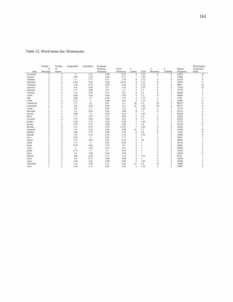
161

Table 12. Word items list: Homonyms

Item

Number

of

Meanings

Number

of

Senses

Imageability

Familiarity

Dominant

Meaning

Frequency

Word

Frequency

#

Letters OLD

#

Phonemes

#

Syllables

Bigram

Frequency

Phonological

Uniqueness

Point

Acontecer 2 3 2 1.57 0.48 0.51 9 2.25 9 4 21875 10

Acuario 2 3 6.69 5.33 0.48 3.77 7 1.85 7 3 27666 8

Alfabeto 2 3 6 5.71 0.71 2.79 8 2.75 8 4 23524 9

Alfombra 2 4 6.65 6.42 0.66 15.43 8 2.15 8 3 19419 9

Atardecer 2 3 5.36 6.73 0.29 6.34 9 2.55 9 4 9892 10

auricular 2 5 6.8 6.29 0.7 1.42 9 2.55 9 4 15526 10

bohemia 2 2 1.77 2.89 0.5 1.1 7 2.7 6 3 12779 7

cardenal 2 4 5.9 2.92 0.71 8.2 8 2.1 8 3 54469 9

casete 2 3 6.69 3.54 0.44 0.59 6 1.5 6 3 40403 7

clip 2 3 6.82 5.7 0.59 1.37 4 1.75 4 1 2728 5

cobra 3 4 6.57 5 0.48 9.19 5 1.15 5 2 43402 6

contención 2 4 1.77 3.5 0.67 4.1 10 2.3 10 3 80379 11

contenedor 2 3 6.8 6.55 0.64 6.4 10 1.95 10 4 80727 11

cromo 2 3 6.6 3.7 0.62 1.52 5 1.45 5 2 13110 6

decorado 2 4 5.2 4.93 0.42 3.66 8 1.7 8 4 92114 9

devenir 2 4 0.88 1.3 0.34 0.25 7 1.95 7 3 85503 8

dicha 2 4 1.7 2.07 0.71 6.94 5 1.6 4 2 14302 5

esconder 2 4 2.71 5.94 0.69 15.6 8 1.7 8 3 83357 9

grafito 2 3 5.25 2.72 0.63 0.28 7 1.85 7 3 22734 8

granito 2 2 5.53 4.37 0.48 1.86 7 1.8 7 3 30728 8

heroína 2 2 4.5 4.75 0.54 17.34 7 2.45 6 4 16295 7

irritación 2 2 3.5 5.42 0.58 0.96 10 2.7 9 4 18358 10

jabalina 2 3 6.66 2.75 0.68 0.32 8 2.8 8 4 17641 9

lanzada 2 4 2.8 4.15 0.54 1.74 7 1.55 7 3 45669 8

lava 2 2 6.07 3 0.61 7.77 4 1 4 2 39971 5

mérito 2 4 1.75 4.93 0.51 6.15 6 1.8 6 3 49081 7

molar 2 4 5.5 4 0.63 0.43 5 1 5 2 30754 6

mona 2 2 6.76 4.61 0.72 9.7 4 1 4 2 26461 5

nodo 2 4 1 1.42 0.72 0.6 4 1 4 2 52818 5

panda 2 2 6.75 4 0.7 6.34 5 1 5 2 32562 6

pinta 3 4 5.5 3.84 0.34 19.8 5 1 5 2 24156 6

plasma 2 4 4.42 4.28 0.73 7.12 6 1.55 6 2 6536 7

soma 2 3 0.8 0.72 0.68 0.49 4 1 4 2 34229 5

sueco 2 5 3.66 3.41 0.38 4.09 5 1.45 5 2 26196 6

viabilidad 2 2 1.55 3.69 0.71 0.42 10 2.5 10 4 15806 5

viola 2 3 6.26 2.11 0.82 4.61 5 1.35 5 2 10987 6

162

Table 13. Word items list: Polysemes

Item

Number

of

Meanings

Number

of Senses

Imageability

Familiarity Word

Frequency # Letters OLD # Phonemes # Syllables Bigram Frequency

Phonological

Uniqueness Point

alarde 1 7 3.5 2.39 1.02 6 1.55 6 3 25732 7

anilla 1 6 5.79 4.09 0.32 6 1.5 5 3 5594 6

balance 1 8 2.57 4.09 5.16 7 1.6 7 3 37142 8

batería 1 13 6.46 6.38 16.36 7 1.7 7 4 47285 8

betún 1 6 5.64 3.5 0.78 5 2 5 2 19786 6

caballito 1 7 6.69 5.08 2.38 9 2.4 8 4 31553 9

caldera 1 12 6.42 4.08 3.24 7 1.7 7 3 39222 8

carbonero 1 9 4.86 2.42 0.35 9 1.85 9 4 43378 10

cargador 1 12 6.67 6.79 4.07 8 1.8 8 3 44952 9

cartón 1 7 6.69 6.27 3.69 6 1.85 6 2 42981 7

cohete 1 7 6.76 5.06 10.47 6 1.85 5 3 37559 6

consulado 1 6 3.5 2.47 4.54 9 1.8 9 4 63954 10

corcho 1 9 6.75 5.33 1.76 6 1.85 5 2 50521 6

corrida 1 9 5 5.55 1.88 7 1.85 6 3 40817 7

cuadrado 1 12 6.87 6.16 4.32 8 1.8 8 3 28254 9

fiador 1 11 1.6 1.85 0.34 6 1.8 6 2 7218 7

fijador 1 6 5 3.27 0.45 7 1.8 7 3 18108 8

filete 1 13 6.8 6.79 7.05 6 1.65 6 3 13080 7

flotador 1 6 6.75 5.39 0.75 8 1.8 8 3 20082 9

furor 1 6 2.25 2.93 0.96 5 1.9 5 2 19913 6

maestría 1 8 2 3.38 1.84 8 2.3 8 4 33989 9

manual 1 14 5.78 5.44 13.56 6 1.9 6 2 24918 7

materia 1 9 3.2 5.11 13.86 7 1.85 7 3 49684 8

músico 1 13 6 6.37 8.62 6 1.9 6 3 17855 7

nube 1 8 6.9 6.70 11.83 4 1.75 4 2 12656 5

obrero 1 8 6.79 5.84 4.35 6 1.8 6 3 28900 7

oreja 1 12 6.91 6.55 15.67 5 1.75 5 3 14933 6

perfil 1 11 5.5 6 16.48 6 1.7 6 2 36767 7

picadura 1 8 5.89 5.875 1.44 8 2.05 8 4 16060 9

plomo 1 6 5.08 4.36 7.61 5 1.7 5 2 4898 6

revés 1 7 2.83 3.87 17.95 5 1.8 5 2 35594 6

rigor 1 8 1.92 2.81 1.73 5 1.9 5 2 162444 6

tormento 1 6 3.4 4.33 2.73 8 1.8 8 3 49766 9

vaina 1 11 6.75 5.06 1.88 5 1.65 5 2 14830 6

vapor 1 6 6 5.41 9.85 5 1.9 5 2 25390 6

zapata 1 9 3.2 2.55 0.42 6 1.8 6 3 12734 7

163

Table 14. Word items list: Hybrids

Item

Number

of

Meanings

Number

of

Senses

Imageability

Familiarity

Dominant

Meaning

Frequency

Word

Frequency

#

Letters OLD

#

Phonemes

#

Syllables

Bigram

Frequency

Phonological

Uniqueness

Point

amanecer 2 9 5.82 6.22 0.44 25.85 8 2 8 4 23243 9

anochecer 2 7 6 6.42 0.18 6.24 9 2.4 8 4 11796 9

botín 2 6 5.6 4.36 0.43 6.87 5 1.7 5 2 10816 6

capitular 2 10 1.4 1.92 0.7 0.22 9 1.85 9 4 25536 10

carpa 3 6 6.23 4.38 0.69 4.73 5 1 5 2 34263 6

chorizo 2 9 6.76 6.52 0.27 1.17 7 1.85 6 3 26160 7

circular 2 12 6 5.13 0.45 4.19 8 1.6 8 3 16835 9

coca 6 12 6 5.83 0.71 14.26 4 1 4 2 38141 5

colonia 2 13 6.76 6.07 0.38 13.32 7 1.7 7 3 53799 8

coral 3 14 5.86 3.33 0.54 4.14 5 1.4 5 2 70465 6

dieta 2 9 3.5 5.84 0.73 11.88 5 1.5 5 2 37266 6

duelo 2 7 3.75 4.47 0.48 10.82 5 1.3 5 2 27082 6

escalar 2 8 5.89 5.88 0.78 5.33 7 1.2 7 3 78961 8

golfo 3 8 4 5.09 0.56 6.43 5 1.8 5 2 9008 6

jota 3 6 5.78 4.11 0.39 1.34 4 1 4 2 25229 5

legado 2 6 1.25 2.46 0.69 8.11 6 1.15 6 3 26561 7

lima 3 9 6.47 4.67 0.3 4.71 4 1 4 2 11916 5

lonja 2 7 5.5 4.06 0.72 0.14 5 1.7 5 2 24466 6

monitor 2 9 5.78 5.84 0.33 6.42 7 1.85 7 3 35712 8

mora 2 7 6.94 4.54 0.72 1.82 4 1 4 2 40288 5

muelle 2 7 6.31 5.13 0.33 16.79 6 1.65 5 2 24832 6

oratorio 2 7 1.63 2.29 0.72 0.18 8 2.35 8 4 25969 9

oscurecer 2 9 5.13 6 0.46 1.07 9 1.7 9 4 15024 10

palmar 2 11 2.4 3.14 0.59 0.3 6 1.25 6 2 37112 7

pica 2 13 3.45 4.31 0.69 6.29 4 1 4 2 7897 5

pilar 3 7 4.27 4.13 0.74 3.7 5 1.1 5 2 21908 6

pino 2 6 6.75 5.75 0.79 4.48 4 1 4 2 10473 5

pipa 2 14 6.9 4.74 0.49 8.14 4 1 4 2 4616 5

pita 4 9 5.29 2.5 0.55 1.55 4 1 4 2 25163 5

polo 3 14 6 5 0.58 10.39 4 1 4 2 32564 5

proceder 2 11 2 4 0.61 6.85 8 1.65 8 3 22002 9

revuelta 2 6 3.33 4.08 0.5 2.99 8 1.65 8 3 24122 9

titular 2 12 4.1 5.27 0.3 4.34 7 1.55 7 3 14433 8

tocado 2 9 5.29 4.83 0.51 19.14 6 1.35 6 3 26927 7

tocador 2 6 6.13 4.2 0.74 2.66 7 1.8 7 3 27689 8

vincular 2 7 2.17 3.8 0.68 0.46 8 1.7 8 3 17255 9

164

Table 15. Nonword items list: Easy Nonwords

Item Letters Phonemes Syllables Bigram Freq OLD acafe 5 5 3 115 1.95

agavo 5 5 3 99 1.95 ahiscaja 8 7 4 857 3.45

ámojo 5 5 3 129 1.95

arlunega 8 8 4 904 3.7 asmur 5 5 2 99 2

atejumo 7 7 4 486 2.95 atusleva 8 8 4 845 3.75

avige 5 5 3 111 2.4

bafega 6 6 3 374 2.55 bailusmo 8 8 3 896 3.55

bebur 5 5 2 137 2.4 beñon 5 5 2 147 2.4

bilócogo 8 8 4 805 3.75

bochunche 9 7 3 888 3.85 bocugo 6 6 3 448 2.8

brembe 6 6 2 427 2.85 brosma 6 6 2 428 1.95

brúrugo 7 7 3 473 3.1

bruruzo 7 7 3 436 3.15 cebigo 6 6 3 488 2.35

chambo 6 5 2 479 1.9

chifeche 8 6 3 878 3.45

climbugir 9 9 3 568 4.85

clirde 6 6 2 324 2.85 clochago 8 7 3 890 3.6

clochigo 8 7 4 785 3.55 creñiz 6 6 2 365 2.85

crumofeco 9 9 4 819 4.35

cumidujo 8 8 4 898 3.75 ecioncer 8 8 3 775 3.6

eclemplía 9 9 4 899 4.05 edeha 5 4 3 81 2.7

edigono 7 7 4 641 2.85

egafiñega 9 9 5 334 4.75 elicefia 8 8 5 867 3.6

eliol 5 5 2 140 2.65 emócoma 7 7 4 553 2.95

epegono 7 7 4 657 2.85

epepoco 7 7 4 439 3.15 epifono 7 7 4 537 2.95

eplubio 7 7 3 405 3.1 equirumbio 10 9 4 607 4.85

ermo 4 4 2 74 1.75

espupo 6 6 3 377 2.2 etonomo 7 7 4 311 2.95

euficimo 8 8 4 845 3.65 evuja 5 5 3 89 2.65

fego 4 4 2 68 1.55

fibó 4 4 2 75 1.75 fluetin 7 7 3 495 3.35

frumaje 7 7 3 689 2.8 frumopeco 9 9 4 851 4.4

gafuz 5 5 2 144 2.65

gizgapana 9 9 4 931 4.5 gloncamiña 10 10 4 853 4.8

glonsadiña 10 10 4 988 4.75

165

glucegia 8 8 3 801 3.55

grumaje 7 7 3 689 2.8 gruruzo 7 7 3 479 3.55

grusaje 7 7 3 675 2.95 guejacho 8 7 3 864 3.55

guetocono 9 9 4 996 4.4

guicho 6 6 2 436 2 gusmeo 6 6 3 420 2.8

gúvucho 7 6 3 384 3.1 hicojo 6 5 3 336 2.7

hiez 4 3 1 60 1.9

hinogo 6 5 3 419 2.55 hiploguil 9 7 3 779 4.9

hochego 7 5 3 668 2.95

hofelzo 7 6 3 606 3.6

hojirzo 7 6 3 578 3.35

ismulema 8 8 4 750 3.65 logiroia 8 8 4 768 3.75

lunu 4 4 2 68 1.95 luño 4 4 2 68 1.7

midirumbia 10 10 4 998 5.15

miosma 6 6 3 342 2.45 muntuaz 7 7 2 729 2.85

negoegia 8 8 4 797 3.6 neucongia 9 9 3 966 3.85

neupe 5 5 2 98 2.75

nevaje 6 6 3 325 2.45 nidorco 7 7 3 749 3

nimopo 6 6 3 257 2.7 nitojo 6 6 3 290 2.7

nochego 7 6 3 656 2.85

nodaza 6 6 3 395 2.3 noiurgo 7 7 3 395 3.1

nopiza 6 6 3 366 2.55 ocaje 5 5 3 84 2

ocuga 5 5 3 139 2.05

odaja 5 5 3 96 1.95 ódogo 5 5 3 127 2.35

odomo 5 5 3 99 1.95 odoso 5 5 3 119 1.95

ojesa 5 5 3 149 1.9

olaña 5 5 3 141 2 oldo 4 4 2 74 1.85

oliña 5 5 3 113 1.95 ordamo 6 6 3 422 2.6

ozoga 5 5 3 122 2.4

plopa 5 5 2 142 1.95 plubleno 8 8 3 800 3.65

plunegio 8 8 3 856 3.6 plurumo 7 7 3 452 3.25

plusije 7 7 3 518 3.25

puel 4 4 1 78 1.85 ragmodio 8 8 3 787 3.45

riapembre 9 9 3 932 3.85 rizoga 6 6 3 205 2.55

rizoja 6 6 3 211 2.4

ruño 4 4 2 74 1.65 sabu 4 4 2 71 2

sañurza 7 7 3 713 2.95 sipimo 6 6 3 399 2.5

sizoma 6 6 3 289 2.7

sozueo 6 6 4 441 2.55

suje 4 4 2 66 2

tezo 4 4 2 73 1.8 todroiga 8 8 3 807 3.65

tofama 6 6 3 463 2.55

166

toñaga 6 6 3 333 2.55

tóñiga 6 6 3 318 2.5 toñima 6 6 3 372 2.55

toñiza 6 6 3 305 2.5 tujé 4 4 2 66 1.95

tuño 4 4 2 66 1.55

uduco 5 5 3 139 2.6 udumo 5 5 3 78 2.6

ulmembre 8 8 3 771 3.6 usuglosco 9 9 4 892 4.55

vaglur 6 6 2 250 2.8

vimunja 7 7 3 591 3.25 visurja 7 7 3 748 2.85

zoiba 5 5 2 110 2

zoima 5 5 2 146 1.95

zojínia 7 7 4 740 3

zuflui 6 6 2 87 3.8 zufú 4 4 2 26 2.4

zuglú 5 5 2 77 2.95 zujón 5 5 2 114 2.9

zulefe 6 6 3 328 2.9

167

Table 16. Nonword items list: Hard Nonwords

Item Letters Phonemes Syllables Bigram Freq OLD

acotador 8 8 4 4530 1.85 arrigada 8 7 4 3708 1.75

arrigado 8 7 4 4376 1.8 bacha 5 4 2 509 1.35

balado 6 6 3 1838 1.45

banada 6 6 3 1648 1.5 bandado 7 7 3 3375 1.65

barada 6 6 3 1925 1.5 barta 5 5 2 754 1.3

bártera 7 7 3 2894 1.7

bérrado 7 6 3 3574 1.7 bosa 4 4 2 145 1

cablado 7 7 3 3589 1.7 cacado 6 6 3 1854 1.55

cacar 5 5 2 799 1.3

cadilla 7 6 3 2522 1.65 cado 4 4 2 155 1

cájada 6 6 3 1623 1.5 cajado 6 6 3 1646 1.55

cajar 5 5 2 692 1.35

caldado 7 7 3 3776 1.6 calgada 7 7 3 3580 1.65

calgado 7 6 3 3858 1.6

calia 5 5 2 817 1.25

calio 5 5 2 785 1.35

calsado 7 7 3 3684 1.65 calsero 7 7 3 2445 1.65

caltado 7 7 3 4183 1.65 caltar 6 6 2 1914 1.45

camado 6 6 3 1776 1.5

camar 5 5 2 752 1.35 camparilla 10 8 4 4960 2.75

cánado 6 6 3 1942 1.45 canar 5 5 2 883 1.2

canera 6 6 3 1867 1.4

cañado 6 6 3 1530 1.5 carada 6 6 3 2196 1.4

carado 6 6 3 2219 1.25 carar 5 5 2 1021 1.35

carco 5 5 2 747 1.25

carleta 7 7 3 2423 1.65 carto 5 5 2 821 1.3

cascador 8 8 3 4663 1.95 castado 7 6 3 4182 1.65

castador 8 8 3 5754 1.85

castar 6 6 2 1908 1.45 celilla 7 6 3 2283 1.65

cona 4 4 2 181 1 cordo 5 5 2 621 1.35

corla 5 5 2 647 1.3

corrada 7 6 3 3899 1.6 corrar 6 5 2 1811 1.5

correta 7 6 3 2748 1.7 corteo 6 6 3 1267 1.5

cortera 7 7 3 3179 1.6

corteró 7 7 3 2710 1.6 cortillá 8 7 3 4610 1.8

cotar 5 5 2 719 1.3

168

cula 4 4 2 147 1

cunta 5 5 2 473 1.35 denencia 8 8 3 3385 1.8

desabrado 9 9 4 9032 2 desacrado 9 9 4 9095 1.9

desatrado 9 9 4 9339 1.9

descerada 9 9 4 8648 2.05 desémbrado 10 10 4 10251 2.7

despectado 10 10 4 11196 2.4 despírada 9 9 4 8351 2.1

destante 8 8 3 7135 1.8

encarlada 9 9 4 6736 1.8 encarlado 9 9 4 7617 1.9

encarmada 9 9 4 6628 1.9

encarmado 9 9 4 7509 1.95

encarpada 9 9 4 6356 2

encarpado 9 9 4 7237 2.05 escacada 8 8 4 4332 1.8

fala 4 4 2 183 1 fana 4 4 2 159 1

holar 5 4 2 649 1.3

leta 4 4 2 170 1 madá 4 4 2 175 1

malada 6 6 3 1964 1.45 manadera 8 8 4 3591 1.8

mandilla 8 7 3 3744 1.8

manté 5 5 2 693 1.35 mantera 7 7 3 3009 1.65

manza 5 5 2 517 1.35 marada 6 6 3 2074 1.45

marado 6 6 3 2097 1.45

margar 6 6 2 1733 1.55 marilla 7 6 3 2915 1.7

mastilla 8 7 3 4079 1.7 menada 6 6 3 1545 1.5

minta 5 5 2 519 1.3

mortillo 8 7 3 3774 1.85 mosa 4 4 2 155 1

mosada 6 6 3 1447 1.5 nallada 7 6 3 3217 1.7

pacada 6 6 3 1649 1.4

pacador 7 7 3 2457 1.65 pajada 6 6 3 1441 1.4

pálado 6 6 3 1927 1.4 pallar 6 5 2 1806 1.5

Pamada 6 6 3 1571 1.3

panilla 7 6 3 2519 1.6 pantá 5 5 2 723 1.3

pantilla 8 7 3 4021 1.65 papador 7 7 3 2212 1.65

parga 5 5 2 700 1.3

partillo 8 7 3 4122 1.85 pasilla 7 6 3 2464 1.6

pazada 6 6 3 1363 1.5 pentada 7 7 3 3617 1.6

pesta 5 5 2 542 1.3

pestante 8 8 3 6272 1.85 ponó 4 4 2 153 1

raca 4 4 2 157 1 racía 5 5 3 507 1.35

ragar 5 5 2 593 1.35

raliente 8 8 3 4468 1.9

ramar 5 5 2 634 1.35

recadora 8 8 4 4557 1.8 recatador 9 9 4 9192 2.1

rementar 8 8 3 4799 1.8

169

reñadora 8 8 4 3670 1.85

resatada 8 8 4 6643 1.8 resatado 8 8 4 7311 1.75

rocado 6 6 3 1438 1.45 ronada 6 6 3 1490 1.55

sallada 7 6 3 3455 1.6

sallado 7 6 3 3733 1.5 sallar 6 5 2 1705 1.45

sentalidad 10 10 4 4326 2.5 soblado 7 7 3 3020 1.65

támada 6 6 3 1431 1.5

tarca 5 5 2 645 1.3 tenta 5 5 2 601 1.25

tonda 5 5 2 535 1.35

tora 4 4 2 187 1

torado 6 6 3 1732 1.55

tota 4 4 2 183 1 traco 5 5 2 414 1.35

valo 4 4 2 170 1 vato 4 4 2 158 1

170

Table 17. Nonword items list: Very Easy Nonwords

Item Letters Phonemes Syllables Bigram Freq OLD adafoafo 8 8 5 289 3

adafoajo 8 8 5 465 4.65 afetrud 7 7 3 337 2.8

agafe 5 5 3 61 2.9

ajarbolu 8 8 4 421 3.1 ajargolu 8 8 4 489 3

ajísfoli 8 8 4 328 2.95 amibuño 7 7 4 470 2.95

amibupo 7 7 4 303 2.95

avolua 6 6 3 170 4 azufe 5 5 3 41 2.9

azuje 5 5 3 71 2.9 azuñe 5 5 3 42 2.8

Bigompo 7 7 3 332 2.9

bíptus 6 6 2 100 3.7 churuotul 9 8 3 664 4

ciñifa 6 6 3 131 2.8 ciñiña 6 6 3 122 2.8

claubun 7 7 2 369 2.8

climbugir 9 9 3 568 2.9 climbumir 9 9 3 574 2.9

cloñofa 7 7 3 330 2.9

dadafumo 8 8 4 426 4

dahidoje 8 7 3 477 3

duenvebeva 10 10 4 658 5 ebecofo 7 7 4 140 3

ebepoco 7 7 4 364 2.9 ebeza 5 5 3 72 2.9

ebigoco 7 7 4 375 3.1

ecajir 6 6 3 160 2.8 ecopus 6 6 3 144 2.9

ectur 5 5 2 57 4.4 edecojo 7 7 4 305 4.65

edefa 5 5 3 48 2.9

edetofo 7 7 4 227 2.9 edetojo 7 7 4 312 4.45

edetoño 7 7 4 343 2.95 edobumo 7 7 4 253 4.45

edopumo 7 7 4 292 2.9

efio 4 4 2 19 2.9 egafiñefa 9 9 5 243 3.95

egafiñema 9 9 5 411 4.8 egir 4 4 2 23 4.85

eglócogo 8 8 4 139 2.9

ehuijoco 8 7 4 414 3 ehuipoco 8 7 4 457 3.1

ejol 4 4 2 10 4.4 eltofrusma 10 10 4 684 4

emofafo 7 7 4 356 2.9

enjin 5 5 2 70 4.4 enul 4 4 2 19 4.4

epicofo 7 7 4 193 3.1 epol 4 4 2 8 3.7

epulsofal 9 9 4 375 2.95

epunsofal 9 9 4 500 4.65 equejavir 9 8 4 616 2.9

equiruzgio 10 9 4 580 4

171

erfapleza 9 9 4 621 2.95

ertún 5 5 2 62 4.4 espur 5 5 2 64 4.4

etocomo 7 7 4 309 3.1 etolomo 7 7 4 328 4.45

etrus 5 5 2 74 4.4

eutobunfo 9 9 4 594 3 éxtul 5 5 2 28 4.4

ezpócofo 8 8 4 75 4 ezpócogo 8 8 4 123 2.9

fafafo 6 6 3 188 2.9

fazifo 6 6 3 170 2.9 fiañipo 7 7 3 321 3.1

fifozafo 8 8 4 490 4.45

fluejua 7 7 2 305 4.4

flufru 6 6 2 136 4.4

flupli 6 6 2 174 4.85 fuayeña 7 7 3 265 2.9

fuodolín 8 8 3 356 4.65 fuonolín 8 8 3 442 4

fuzgolín 8 8 3 324 2.9

gefozafo 8 8 4 455 3.1 gefozaño 8 8 4 701 2.95

glurugo 7 7 3 359 2.9 Glurumo 7 7 3 342 2.9

gluruzo 7 7 3 322 2.8

ibiol 5 5 2 53 2.9 ibión 5 5 2 21 2.9

ifri 4 4 2 26 4.85 igiol 5 5 2 44 2.9

imbú 4 4 2 24 4.4

indur 5 5 2 74 4.85 iñao 4 4 3 6 4.85

ipioga 6 6 3 126 2.95 ipiol 5 5 2 58 2.8

irbu 4 4 2 27 4.4

jaflui 6 6 2 135 4.4 jauruñín 8 8 3 348 3.1

jezoña 6 6 3 94 4.45 jezopa 6 6 3 128 2.9

jezova 6 6 3 129 2.9

jideñafa 8 8 4 332 2.9 jiugon 6 6 2 160 4.4

juzgin 6 6 2 181 4.4 nefoñaño 8 8 4 565 4.4

noausmo 7 7 3 301 2.9

nuju 4 4 2 28 4.4 nuvugo 6 6 3 118 2.8

ocañe 5 5 3 80 2.9 ocijín 6 6 3 79 2.8

ocijus 6 6 3 115 2.8

ocimin 6 6 3 173 2.9 ocobul 6 6 3 109 2.9

ocofol 6 6 3 119 2.9 ocoñol 6 6 3 145 2.8

ocufa 5 5 3 62 2.8

ofaude 6 6 3 178 2.8 ofiode 6 6 3 158 4.65

ogue 4 3 2 9 4.4 oibur 5 5 2 62 4.4

oidur 5 5 2 73 4.4

oldosus 7 7 3 357 2.9

oldu 4 4 2 27 4.4

oliazmudio 10 10 4 565 6 onmehimo 8 7 3 495 2.95

plubu 5 5 2 77 4.4

172

plubul 6 6 2 146 4.4

rujiroigo 9 9 4 561 3.1 runjun 6 6 2 195 4.85

rusdun 6 6 2 152 4.85 rusnun 6 6 2 153 4.4

ruspun 6 6 2 163 3.7

uchur 5 4 2 32 4.4 udujo 5 5 3 67 2.9

ulfe 4 4 2 18 4.85 ulluo 5 4 2 32 2.8

ulpe 4 4 2 28 4.4

umodofa 7 7 4 152 3 umodoma 7 7 4 269 4.25

ursu 4 4 2 26 4.4

usuclucto 9 9 4 699 2.8

zaibrí 6 6 2 185 2.8

zijie 5 5 2 74 2.9 zufru 5 5 2 63 4.4

zuglu 5 5 2 77 4.85 zupli 5 5 2 79 4.4

zutrui 6 6 2 195 3.7

173

Appendix 2

2.1. Summary of statistical analysis for the behavioural investigations

Table 18. Complete statistics for the full models applied to the RT data from behavioural investigations

Experiment

Visual Lexical Decision: Nonword

Wordlikeness (Easy/ Hard Nonwords)

Visual Lexical Decision: Visual Noise

Intermodal Lexical Decision Auditory Lexical Decision: Auditory

Noise

Auditory Lexical Decision:

Compression/Expansion

β SE t p β SE t p β SE t p β SE t p β SE t p Manipulation 46.19 19.47 2.37 .01 378.63 12.86 29.42 <.0001 302.25 8.54 35.38 <.0001 53.42 8.22 6.49 <.0001 186.78 9.78 19.09 <.0001

Homonyms 8.71 9.33 0.93 .35 8.28 13.59 0.60 .54 25.10 10.25 2.44 .01 35.63 14.87 2.39 .01 13.39 16.50 0.81 .41

Hybrid -5.14 10.11 -0.50 .61 -2.16 14.72 -0.14 .88 8.08 11.10 0.72 .46 0.69 16.15 0.04 .96 -13.40 18.03 -0.74 .45

Polysemes -19.79 9.34 -2.11 .04 -16.75 13.60 -1.23 .21 -8.39 10.26 -0.81 .41 2.52 14.87 0.17 .86 7.28 16.58 0.43 .66

Imageability -17.51 3.38 -5.17 <.0001 -16.54 4.91 -3.36 <.001 -16.57 3.73 -4.43 <.0001 -20.47 5.41 -3.78 <.001 -11.22 6.08 -1.84 .07

Homonyms:manipulation 13.14 8.23 1.59 .11 7.20 16.45 0.43 .66 10.31 10.76 0.95 .33 13.52 11.47 1.17 .23 29.71 13.19 2.25 .02

Hybrid:manipulation -6.41 8.89 -0.72 .47 -19.74 17.64 -1.11 .26 -14.11 11.62 -1.21 .22 -6.50 12.34 -0.52 .59 5.02 14.40 0.34 .72

Polysemes:manipulation 1.31 8.23 0.16 .87 30.71 16.26 1.88 .06 12.41 10.75 1.15 .24 -9.16 11.35 -0.80 .41 -6.52 13.29 -0.49 .62

Imageability:manipulation -0.98 2.99 -0.32 .74 -9.33 5.94 -1.57 .11 -5.61 3.93 -1.42 .15 -5.51 4.15 -1.32 .18 -8.39 4.88 -1.71 .09

Table 19. Complete statistics for the pairwise models applied to the RT data from behavioural investigations

Visual Lexical Decision: Nonword

Wordlikeness (Easy/ Hard Nonwords)

Visual Lexical Decision: Visual

Noise Intermodal Lexical Decision

Auditory Lexical Decision:

Auditory Noise

Auditory Lexical Decision:

Compression/Expansion

Condition analyzed β SE t p β SE t P β SE t p β SE t p β SE t p Homonyms Baseline 9.05 8.62 1.05 .29 7.11 9.23 0.77 .44 25.44 9.33 2.72 <.01 34.74 13.44 2.58 .01 7.89 20.23 0.39 .69

Hybrid Baseline -4.64 9.35 -0.49 .62 -2.95 10.00 -0.29 .76 8.48 10.10 0.83 .40 -0.36 14.60 -0.02 .97 -10.09 22.13 -0.45 .64

Polysemes Baseline -19.41 8.64 -2.24 .03 -18.23 9.24 -1.97 .05 -8.12 9.34 -0.87 .38 2.14 13.45 0.15 .87 3.72 20.25 0.18 .85

Imageability Baseline -17.58 3.13 -5.61 <.0001 -16.17 3.36 -4.80 <.0001 -17.26 3.40 -5.06 <.0001 -20.00 4.93 -4.05 <.0001 -8.82 7.45 -1.18 .23

Homonyms Slowed 21.26 11.11 1.91 .06 12.88 20.46 0.62 .53 34.32 13.88 2.47 .01 53.23 17.60 3.02 <.01 43.81 18.50 2.36 .02

Hybrids Slowed -12.07 12.05 -1.00 .31 -22.46 21.98 -1.02 .30 -5.24 15.05 -0.34 .72 -5.61 19.03 -0.29 .76 -8.32 20.09 -0.41 .67

Polysemes Slowed -18.77 11.12 -1.68 .09 11.15 20.24 0.55 .58 3.48 13.89 0.25 .80 -6.49 17.53 -0.37 .71 1.15 18.54 0.06 95

Imageability Slowed -18.29 4.03 -4.53 <.0001 -23.99 7.29 -3.28 <.01 -21.67 5.06 -4.28 <.0001 -26.65 6.33 -4.20 <.0001 -19.53 6.78 -2.88 <.01

174

Table 20. Complete statistics for the full models applied to the ACC data from behavioural investigations

Visual Lexical Decision: Nonword

Wordlikeness (Easy/ Hard Nonwords)

Visual Lexical Decision: Visual

Noise Intermodal Lexical Decision

Auditory Lexical Decision: Auditory

Noise

Auditory Lexical Decision:

Compression/Expansion

β SE z p β SE z p β SE z p β SE z p β SE z p

Manipulation < .01 0.26 0.01 .98 -1.65 0.21 -7.83 <.0001 3.66 0.27 13.12 <.0001 -2.20 0.26 -8.31 <.0001 2.02 0.24 8.34 <.0001

Homonyms -0.09 0.30 -0.30 .75 -0.17 0.30 -0.55 .58 -0.02 0.34 -0.07 .94 -0.91 0.40 -2.25 .02 0.63 0.60 1.04 .29

Hybrid 0.25 0.30 0.81 .41 0.14 0.32 0.45 .64 0.30 0.35 0.85 .39 -0.73 0.41 -1.78 .07 -0.66 0.58 -1.13 .25

Polysemes 0.40 0.31 1.28 .20 -0.08 0.31 -0.27 .78 0.25 0.36 0.70 .47 -0.53 0.42 -1.24 .21 0.10 0.59 0.18 .85

Imageability 0.40 0.10 3.73 <.001 0.36 0.10 3.43 <.0001 0.35 0.12 2.84 <.01 0.21 0.14 1.54 .12 0.15 0.21 0.74 .45

Homonyms:manipulation -0.30 0.22 -1.32 .18 <0.01 0.28 <0.01 .99 -0.10 0.37 -0.26 .78 1.03 0.33 3.08 <.01 -0.79 0.34 -2.34 .02

Hybrid:manipulation -0.45 0.23 -1.91 .06 0.07 0.30 0.24 .80 -0.36 0.39 -0.92 .35 0.91 0.34 2.68 <.01 0.27 0.33 0.79 .42

Polysemes:manipulation -0.32 0.24 -1.31 .18 0.23 0.30 0.77 .43 -0.13 0.40 -0.34 .73 1.15 0.36 3.16 <.01 -0.51 0.33 -1.54 .12

Imageability:manipulation 0.02 0.08 0.33 .73 -0.09 0.10 -0.97 .33 0.08 0.13 0.64 .52 -0.02 0.11 -0.25 .79 0.20 0.12 1.68 .09

Table 21. Complete statistics for the pairwise models applied to the ACC data from behavioural investigations

Visual Lexical Decision: Nonword

Wordlikeness (Easy/ Hard Nonwords)

Visual Lexical Decision: Visual

Noise Intermodal Lexical Decision

Auditory Lexical Decision:

Auditory Noise

Auditory Lexical Decision:

Compression/Expansion

Condition analyzed β SE z p β SE z p β SE z p β SE z p β SE z p

Homonyms Baseline -0.01 0.30 0.25 .98 -0.31 0.43 -0.73 .46 0.04 0.38 -0.12 .89 -0.85 0.39 -2.17 .03 0.80 0.75 1.06 .28

Hybrid Baseline 0.28 0.30 0.94 .34 0.12 0.44 0.28 .77 0.24 0.39 0.62 .53 -0.51 0.40 1.29 .19 -0.70 0.71 -0.98 .32

Polysemes Baseline 0.39 0.31 1.24 .21 -0.10 0.44 0.24 .80 0.26 0.40 0.66 .50 -0.23 0.42 -0.56 .57 0.01 0.73 0.01 .98

Imageability Baseline 0.42 0.10 3.93 <.0001 0.40 0.15 2.64 <.01 0.38 0.13 2.78 <.01 0.22 0.14 1.59 .11 0.29 0.26 1.13 .25

Homonyms Slowed -0.33 0.35 -0.94 .34 -0.17 0.22 -0.76 .44 -0.02 0.34 -0.07 .93 0.10 0.39 0.26 .79 -0.20 0.50 -0.40 .68

Hybrids Slowed -0.21 0.35 -0.60 .54 0.25 0.22 1.10 .27 0.12 0.34 0.35 .72 0.09 0.39 0.25 .80 -0.42 0.49 -0.85 .39

Polysemes Slowed 0.05 0.37 0.16 .87 0.15 0.23 0.68 .49 0.18 0.36 0.51 .60 0.50 0.40 1.23 .21 0.01 0.51 0.01 1

Imageability Slowed 0.44 0.12 3.50 <.0001 0.26 0.08 3.23 <.01 0.44 0.12 3.61 <.001 0.22 0.14 1.59 .11 0.15 0.17 0.83 .40

175

Appendix 3

3.1. Supplemental Statistics for the Very Easy nonword condition

The methods used for the very easy nonword condition were the same as those used

in each of the conditions in the nonword wordlikeness experiment. The very easy

nonword condition was completed by 42 new participants.

Table 22. Detailed stimuli descriptive statistics of words in comparison to nonword stimuli sets

Bigram Frequency Levenshtein Distance Coltheart N Number of Letters

Min - Max Mean (SE) Min - Max Mean (SE) Min - Max Mean (SE) Min - Max Mean (SE)

Words 36 - 7719 1602 (130) 0.9 - 3.6 2.0 (0.05) 0 - 18 2.4 (0.31) 4 - 10 6.5 (0.12)

Very Easy 6 - 701 231 (16) 2.8 – 6.0 3.6 (0.06) 0 - 2 0.03 (0.01) 4 - 10 6.5 (0.12)

Easy 26 - 998 446 (25) 1.5 - 5.2 2.9 (0.07) 0 - 3 0.31 (0.06) 4 - 10 6.5 (0.12)

Hard 145 - 11196 2783 (205) 1 - 2.8 1.5 (0.03) 0 - 18 4.61 (0.33) 4 - 10 6.5 (0.12)

Table 23. Averages and standard error for Reaction Times and Accuracy in the three conditions of the

nonword wordlikeness experiment

Reaction Times Accuracy

M (SE) Very Easy Easy Hard Very Easy Easy Hard

Unambiguous 642 (4.7) 644 (4.7) 690 (5.6) 96.7 (0.5) 93.6 (0.6) 94.0 (0.6)

Homonym 651 (5.3) 654 (5.3) 717 (5.9) 96.7 (0.5) 94.6 (0.6) 94.0 (0.7)

Hybrid 620 (4.5) 618 (4.5) 675 (5.0) 97.7 (0.4) 95.8 (0.5) 94.3 (0.6)

Polyseme 625 (4.6) 617 (4.6) 667 (5.0) 97.7 (0.4) 95.8 (0.5) 95.0 (0.6)

Nonword 708 (3.0) 731 (3.0) 831 (3.4) 96.2 (0.3) 95.1 (0.3) 92.7 (0.4)

176

3.2. Results of additional analyses involving the very easy nonwords

The data were analyzed in the same manner described in the main text. For

simplicity, we report the analyses run on the very easy nonword condition in isolation

first.

Within-condition analyses. Correct latency. There was only a marginal

polysemy advantage (b = -11.75, SE = 7.83, t = -1.50, p =.13) and a significant main

effect for imageability (b = -11.16, SE = 2.85, t = -3.90, p < .001).

Accuracy. No significant or marginal effects were detected. Accuracy was closer

to ceiling in this condition than in any of the other conditions analyzed in the main text.

Between-condition analyses. We ran two sets of analyses, each time using the

very easy nonwords as the baseline condition, and either the easy nonwords or the hard

nonwords as the slowed condition.

Correct latency. In the analyses of the [very easy vs. easy] data, there was a

marginal there was a marginal overall polysemy advantage (b = -11.72, SE = 8.03, t = -

1.45, p =.14) and a significant main effect for imageability (b = -11.21, SE = 2.92, t = -

3.83, p < .001). There was no significant main effect of difficulty, and numerically the

latencies were very similar for all ambiguity types across the two levels of difficulty. In

the analysis of the [very easy vs. hard] data, responses were significantly slower overall

in the hard nonword condition (b = 45.71, SE = 18.071, t = 2.44, p =.01), there were

also marginal interactions between the slowing manipulation and homonyms, indicating

a larger homonym disadvantage in the slower condition (b = 12.55, SE = 8.31, t = 1.51,

p =.13), and between the slowing manipulation and hybrid items, indicating a larger

hybrid advantage in the slower condition (b = -16.96, SE = 8.99, t = -1.88, p = .06).

177

There was also a significant main effect of imageability (b = -11.09, SE = 3.16, t = -3.50,

p < .001) and an interaction between the slowing manipulation and imageability (b = -

7.59, SE = 3.02, t = -2.51, p = .01) .

Accuracy. Both the [very easy vs. easy] model and the the [very easy vs. hard]

model failed to converge. This is not entirely unexpected given the near-ceiling levels of

accuracy, particularly in the very easy nonword condition.

Additionally, although our primary focus has been on performance for the word

stimuli, it is worth noting that the slowing manipulation also appears to have had an

effect on nonword performance that varied across the three level of nonword difficulty.

Whereas the difference between very easy and easy nonwords was relatively small (23

ms), the difference was much larger (100 ms) between easy and hard nonwords. This

observation is broadly consistent with the analyses of the word data outlined above,

which indicated a high level of similarity in performance between very easy and easy

nonword conditions, and larger differences when these conditions were contrasted to the

hard nonword condition. This in turn suggests that despite the relatively large change in

nonword difficulty, there is a floor effect of the effect of nonword difficulty when

manipulating bigram frequency and neighbourhood size, but nevertheless requiring

similar subsyllabic segments and transition frequencies as in real words. A more

extreme manipulation of nonword wordlikeness may therefore be necessary to

substantially improve overall performance, although doing so may also risk decreasing

semantic effects overall (for additional discussion, see also Armstrong & Plaut, 2016;

Azuma & Van Orden, 1997; Rodd et al., 2002).

178

Appendix 4

4.1. Ambiguity Type data analysis. N400 effects (250 – 600 ms): Trials with

no Repetitions

The aim of this set of analyses was assessing the neural activity (in microvolts) in

the selected channels (Cz, Pz and Fz) for only the first trial of appearance of each item.

This is, only the first four blocks of the experiment. Similar to the execution of the

behavioural experiments in part I.

4.1.1. Ambiguity Type data analysis. N400 effects (250 – 600 ms): Cz channel –

Trials with no Repetitions

The next analysis focused on predicting the neural activity (in microvolts) in the

Cz channel as a function of fixed effects of ambiguity type (an unambiguous word

baseline vs. homonyms, hybrids, and polysemes) and manipulation (Baseline and

Slowed, in this experiment, respectively clean trials vs visually noisy trials). To address

potential confounds, fixed effects of imageability, residual familiarity, log-transformed

word frequency, Orthographic Levenshtein Distance (OLD), length in letters, and

bigram frequency were also included. Further, to reduce possible auto-correlation effects

from previous trials (Baayen & Milin, 2010), fixed effects of trial number, previous trial

lexicality, previous trial response laterality, previous trial accuracy, and previous trial

reaction time were also added to the model. All continuous variables were centered and

179

normalized (Jaeger, 2010). The model also included random effects of item and

participant.

The results of the full model only revealed a main effect for manipulation (b =-

2.33, SE= 0.64, t =-3.60, p<.0001).

The pairwise tests only revealed one effect significant under bonferroni corrected

p value multiple comparisons; there was a homonym advantage at slowed (noise)

condition the unambiguous vs homonym contrast (b= 1.69, SE= 0.59, t = 2.87, p=.004).

The reported pairwise effect was significant at the bonferroni corrected p value p

≤.008.

Table 24. Ambiguity Type data analysis. N400 effects (250 – 600 ms): Cz channel – Trials with no

Repetitions

Cz Baseline Slowed

β SE t p β SE t p

Homonyms -0.54 0.57 -0.95 .34 1.69 0.59 2.87 .004

Polysemes -0.79 0.60 -1.31 .19 1.57 0.60 2.57 .010

Hybrids -0.36 0.68 -0.52 .60 1.82 0.68 2.67 .0081

180

4.1.2. Ambiguity Type data analysis. N400 effects (250 – 600 ms): Pz channel –

Trials with no Repetitions

The results of the full model only revealed a main effect for manipulation (b =-

1.56, SE= 0.63, t =-2.48, p=.01). There were no other significant or marginal effects.

The pairwise tests revealed none significant effects under bonferroni corrected p

value multiple comparisons (p ≤.008).

Table 25. Ambiguity Type data analysis. N400 effects (250 – 600 ms): Pz channel – Trials with no

Repetitions

Pz Baseline Slowed

β SE t p β SE t P

Homonyms -0.47 0.56 -0.84 .40 0.87 0.58 1.50 .13

Polysemes -0.68 0.57 -1.18 .23 0.75 0.58 1.29 .19

Hybrids -0.50 0.64 -0.77 .44 0.91 0.64 1.41 .15

181

4.1.3. Ambiguity Type data analysis. N400 effects (250 – 600 ms): Fz channel –

Trials with no Repetitions

The results of the full model only revealed a main effect for manipulation (b =-

2.51, SE= 0.70, t =-3.55, p<.001). There were no other significant or marginal effects.

The pairwise tests only revealed one effect significant under bonferroni corrected

p value multiple comparisons; there was a homonym advantage at slowed (noise)

condition the unambiguous vs homonym contrast (b= 1.74, SE= 0.63, t = 2.74, p=.006).

The reported pairwise effect was significant at the bonferroni corrected p value p

≤.008.

Table 26. Ambiguity Type data analysis. N400 effects (250 – 600 ms): Fz channel – Trials with no

Repetitions

Fz Baseline Slowed

β SE t p β SE t P

Homonyms -0.79 0.61 -1.29 .19 1.74 0.63 2.74 .006

Polysemes -0.79 0.66 -1.18 .23 1.79 0.68 2.62 .009

Hybrids -0.58 0.74 -0.78 .43 1.91 0.75 2.53 .012

182

Appendix 5

5.1 Abbreviations’ list

ANOVA Analysis of variance

EEG Electroencephalography

ERP Event Related Potential

Hz Hertz

ICA Independent component analysis

LDT Lexical Decision Task

NoM Number of meanings

NoS Number of senses

OLD Orthographic Levenshtein Distance

RAE Real Academia Española

RTs Reactions Times

SD Standard Deviation

SE Standard Error

SOS Stimulus optimization software

SSD Semantic Settling Dynamics

μV Microvolts

References

Allen, M., Badecker, W., & Osterhout, L. (2003). Morphological analysis in sentence processing:

An ERP study. Language and Cognitive Processes, 18(4), 405-430.

Ardila, A., & Cuetos, F. (2016). Applicability of dual-route reading models to Spanish.

Psicothema, 28(1).

Arduino, L. S., & Burani, C. (2004). Neighborhood effects on nonword visual processing in a

language with shallow orthography. Journal of Psycholinguistic Research, 33(1), 75-95.

Armstrong, B. C. (2012). The temporal dynamics of word comprehension and response selection:

Computational and behavioral studies (Doctoral dissertation). Psychology Department,

Carnegie Mellon University, Pittsburgh. Retrieved from

http://www.blairarmstrong.net/papers/Armstrong.12.DISSERTATION.html

Armstrong, B. C. (2013). Calculating Summed Token (or Type) Length-Specific Positional Bigram

Frequency, Letter (Unigram) Frequency, and Bigram and Letter Legality [Computer

Software]. Retrieved from http://www.blairarmstrong.net/tools/index.html#Bigram

Armstrong, B. C., & Plaut, D. C. (2016). Disparate semantic ambiguity effects from semantic

processing dynamics rather than qualitative task differences. Language, Cognition and

Neuroscience, 31(7), 940-966.

Armstrong, B. C., Watson, C. E., & Plaut, D. C. (2012). SOS! An algorithm and software for the

stochastic optimization of stimuli. Behavior Research Methods, 44(3), 675-705.

Armstrong, B. C., Zugarramurdi, C., Cabana, Á., Lisboa, J. V., & Plaut, D. C. (2015). Relative

meaning frequencies for 578 homonyms in two Spanish dialects: A cross-linguistic

extension of the English eDom norms. Behavior Research Methods, 1-13.

184

Baayen, R.H., Milin, P. (2010). Analyzing Reaction Times. International Journal of Psychological

Research, 3(2), 12-28.

Balota, D. A., & Chumbley, J. I. (1984). Are lexical decisions a good measure of lexical access?

The role of word frequency in the neglected decision stage. Journal of Experimental

Psychology: Human perception and performance, 10(3), 340.

Baluch, B., & Besner, D. (1991). Visual word recognition: Evidence for strategic control of lexical

and nonlexical routines in oral reading. Journal of Experimental Psychology: Learning,

Memory, and Cognition, 17(4), 644.

Bates, D., Maechler, M., Bolker, B., Walker, S. (2015). Fitting Linear Mixed-Effects Models

Using lme4. Journal of Statistical Software, 67(1), 1-48.

Bear, M. F., Connors, B. W., & Paradiso, M. A. (2007). Brain Rhythms and Sleep. In M. F. Bear,

B. W. Connors, & M. A. Paradiso (Eds.), Neuroscience: Exploring the Brain (pp. 601-604)

(3rd ed.). Philadelphia: Lippincott Williams & Wilkins.

Becker, C. A., & Killion, T. H. (1977). Interaction of visual and cognitive effects in word

recognition. Journal of Experimental Psychology: Human Perception and Performance,

3(3), 389.

Beekhuizen, B., Milic, S., Armstrong, B. C., & Stevenson, S. (2018). What Company Do

Semantically Ambiguous Words Keep? Insights from Distributional Word Vectors.

Proceedings of the 40th Annual Conference of the Cognitive Science Society. Mahwah,

NH: Lawrence Erlbaum Associates.

Bentin, S., McCarthy, G., & Wood, C. C. (1985). Event-related potentials, lexical decision and

semantic priming. Electroencephalography and clinical Neurophysiology, 60(4), 343-355.

Beretta, A., Fiorentino, R., & Poeppel, D. (2005). The effects of homonymy and polysemy on

lexical access: An MEG study. Cognitive Brain Research, 24(1), 57-65.

185

Bialystok, E., Craik, F., & Luk, G., (2008). Cognitive control and lexical access in younger and

older bilinguals. Journal of Experimental Psychology: Learning, Memory, and Cognition,

34 (4), 859-873.

Borowsky, R., & Besner, D. (1991). Visual word recognition across orthographies: On the

interaction between context and degradation. Journal of Experimental Psychology:

Learning, Memory, and Cognition, 17(2), 272.

Borowsky, R., & Besner, D. (1993). Visual word recognition: a multistage activation model.

Journal of Experimental Psychology: Learning, Memory, and Cognition, 19(4), 813.

Brown, C., & Hagoort, P. (1993). The processing nature of the N400: Evidence from masked

priming. Journal of Cognitive Neuroscience, 5(1), 34-44.

Brown, S. W. (2008). Polysemy in the mental lexicon. Colorado Research in Linguistics, 21(1), 1-

12.

Buzsáki, G. (2006). Rhythms of the Brain. New York: Oxford University Press.

Canty, A. & Ripley, B. (2016). boot: Bootstrap R (S-Plus) Functions. R package version 1.3-18.

Carreiras, M., Armstrong, B. C., Perea, M., & Frost, R. (2014). The what, when, where, and how

of visual word recognition. Trends in Cognitive Sciences, 18(2), 90-98.

Casanova, C. P. R. (2017). ¿Cómo separan y ordenan las acepciones los diccionarios de lengua

española?. Tonos Digital, (32), 1-38.

Comesaña, M., Ferré, P., Romero, J., Guasch, M., Soares, A. P., & García-Chico, T. (2015).

Facilitative effect of cognate words vanishes when reducing the orthographic overlap: The

role of stimuli list composition. Journal of Experimental Psychology: Learning, Memory,

and Cognition, 41(3), 614.

186

Da Silva, F. L. (2009). EEG: Origin and measurement. In Mulert, C., & Lemieux, L. (Eds.). EEG-

fMRI: physiological basis, technique, and applications (pp. 19-38). Springer. DOI:

10.1007/978-3-540-87919-0

Dahan, D., & Magnuson, J. S. (2006). Spoken word recognition. In M. Traxler, M.A. Gernsbacher

(Eds.), Handbook of Psycholinguistics (pp. 249-283) (2nd

ed.). London, UK: Elsevier.

Debruille, J. B., Ramirez, D., Wolf, Y., Schaefer, A., Nguyen, T. V., Bacon, B. A., Louis Renoult

& Brodeur, M. (2008). Knowledge inhibition and N400: a within-and a between-subjects

study with distractor words. Brain Research, 1187, 167-183.

Degani, T., & Tokowicz, N. (2013). Cross-language influences: Translation status affects

intraword sense relatedness. Memory & Cognition, 41(7), 1046-1064.

Degani, T., Prior, A., Eddington, C. M., da Luz Fontes, A. B. A., & Tokowicz, N. (2016).

Determinants of translation ambiguity. Linguistic Approaches to Bilingualism, 6(3), 290-

307.

DeLong, K. A., Urbach, T. P., & Kutas, M. (2005). Probabilistic word pre-activation during

language comprehension inferred from electrical brain activity. Nature Neuroscience, 8(8),

1117.

Dijkstra, T., & Van Heuven, W. J. B. (1998). The BIA model and bilingual word recognition. In J.

Gainger & A. Jacobs (Eds.), Localist connectionist approaches to human cognition (pp.

189-225). Mahwah, New Jersey: Lawrence Erlbaum Associates.

Domalski, P., Smith, M. E., & Halgren, E. (1991). Cross-modal repetition effects on the N4.

Psychological Science, 2(3), 173-178.

Dowle, M., Srinivasan, A., Short, T., Lianoglou, S., Saporta, R., & Antonyan, E. (2015). data.table:

Extension of Data.frame. R package version 1.9.6. Retrieved from https://CRAN.R-

project.org/package=data.table

187

Duchon, A., Perea, M., Sebastián-Gallés, N., Martí, A., & Carreiras, M. (2013). EsPal: One-stop

shopping for Spanish word properties. Behavior Research Methods, 45(4), 1246-1258.

Duncan-Johnson, C. C., & Donchin, E. (1982). The P300 component of the event-related brain

potential as an index of information processing. Biological Psychology, 14(1), 1-52.

Eddington, C. M., & Tokowicz, N. (2015). How meaning similarity influences ambiguous word

processing: the current state of the literature. Psychonomic Bulletin & Review, 22(1), 13-37.

Federmeier, K. D., Segal, J. B., Lombrozo, T., & Kutas, M. (2000). Brain responses to nouns,

verbs and class-ambiguous words in context. Brain, 123(12), 2552-2566.

Feldman, L. B., & Basnight-Brown, D. M. (2007). Origins of cross language differences in word

recognition. In G. Jarema & G. Libben (Eds.), The mental lexicon: Core perspectives (pp.

129-158). Amsterdam, Netherlands: Elsevier.

Feldman, L. B., & Basnight-Brown, D. M. (2008). List context fosters semantic processing:

parallels between semantic and morphological facilitation when primes are forward

masked. Journal of Experimental Psychology: Learning, Memory, and Cognition, 34(3),

680.

Fontes, A. B. A. D. L., & Schwartz, A. I. (2015). Bilingual access of homonym meanings:

Individual differences in bilingual access of homonym meanings. Bilingualism: Language

and Cognition, 18(04), 639-656.

Fraga, I., Padrón, I., Perea, M., & Comesaña, M. (2016). I saw this somewhere else: The Spanish

Ambiguous Words (SAW) database. Lingua. 185, 1-10.

Frazier, L., & Rayner, K. (1990). Taking on semantic commitments: Processing multiple meanings

vs. multiple senses. Journal of Memory and Language, 29(2), 181.

188

Frost, R. (1994). Prelexical and postlexical strategies in reading: Evidence from a deep and a

shallow orthography. Journal of Experimental Psychology-Learning Memory and

Cognition, 20(1), 116-129.

Frost, R., Katz, L., & Bentin, S. (1987). Strategies for visual word recognition and orthographical

depth: a multilingual comparison. Journal of Experimental Psychology: Human Perception

and Performance, 13(1), 104.

Gilbert, R. A., Davis, M. H., Gaskell, M. G., & Rodd, J. M. (2018). Listeners and readers

generalize their experience with word meanings across modalities. Journal of Experimental

Psychology: Learning, Memory, and Cognition, 44(10), 1533-1561.

GoldWave (v6.13) [computer software]. St. John's, NF: GoldWave ® Inc.

Gollan, T. H. Montoya, R. I., Cera, C., & Sandoval, T. C. (2008). More use almost always means a

smaller frequency effect: Aging, bilingualism, and the weaker links hypothesis. Journal of

Memory and Language, 58, 787-814.

Gollan, T. H., Fennema-Notestine, C., Montoya, R. I., & Jernigan, T. L. (2007). The bilingual

effect on Boston Naming Test performance. Journal of the International

Neuropsychological Society, 13, 197-208.

Grillon, C., Ameli, R., & Glazer, W. M. (1991). N400 and semantic categorization in

schizophrenia. Biological Psychiatry, 29(5), 467-480.

Haas, L. F. (2003). Hans Berger (1873–1941), Richard Caton (1842–1926), and

electroencephalography. Journal of Neurology, Neurosurgery & Psychiatry, 74(1), 9-9.

Hagoort, P., Brown, C. M., & Osterhout, L. (1999). The neurocognition of syntactic processing. In

C. M. Brown & P. Hagoort (Eds.) The Neurocognition of Language (pp. 273-317). New

York: Oxford University Press.

189

Hargreaves, I. S., Pexman, P. M., Pittman, D. J., & Goodyear, B. G. (2011). Tolerating Ambiguity.

Experimental Psychology. 58, 19 – 30.

Haro, J., Demestre, J., Boada, R., & Ferré, P. (2017). ERP and behavioral effects of semantic

ambiguity in a lexical decision task. Journal of Neurolinguistics, 44, 190-202.

Haro, J., Ferré, P., Boada, R., & Demestre, J. (2017). Semantic ambiguity norms for 530 Spanish

words. Applied Psycholinguistics, 38(2), 457-475.

Hawelka, S., Schuster, S., Gagl, B., & Hutzler, F. (2015). On forward inferences of fast and slow

readers. An eye movement study. Scientific Reports, 5, 8432.

Heil, M., Rolke, B., & Pecchinenda, A. (2004). Automatic Semantic Activation Is No Myth

Semantic Context Effects on the N400 in the Letter-Search Task in the Absence of

Response Time Effects. Psychological Science, 15(12), 852-857.

Hino, Y., Kusunose, Y., & Lupker, S. J. (2010). The relatedness-of-meaning effect for ambiguous

words in lexical-decision tasks: When does relatedness matter?. Canadian Journal of

Experimental Psychology/Revue canadienne de psychologie expérimentale, 64(3), 180.

Hino, Y., Pexman, P. M., & Lupker, S. J. (2006). Ambiguity and relatedness effects in semantic

tasks: Are they due to semantic coding?. Journal of Memory and Language, 55(2),

247-273.

Højsgaard, S. & Halekoh, U. (2016). doBy: Groupwise Statistics, LSmeans, Linear Contrasts,

Utilities. R package version 4.5-15. Retrieved from https://CRAN.R-

project.org/package=doBy

Holcomb, P. J. (1993). Semantic priming and stimulus degradation: Implications for the role of the

N400 in language processing. Psychophysiology, 30(1), 47-61.

190

Holcomb, P. J., & Kounios, J. (1990). Semantic memory: An ERP and reaction time analysis. In

C.H. M. Brunia, A.W.K. Gaillard, & A. Kok (Eds), Psychophysiological brain research,

(pp. 285-288). The Netherlands: Tilburg University Press.

Holley-Wilcox, P. (1977). The effect of homophony with auditory presentation of stimuli. Paper

presented at the Meeting of the Midwestern Psychological Association, Chicago, May 1977.

Hubel, D. H., & Wiesel, T. N. (1959). Receptive fields of single neurons in the cat's striate cortex.

The Journal of Physiology, 148(3), 574-591.

Jaeger, T. F. (2010). Common issues and solutions in regression modelling (mixed or not).

Presentation at Brain and Cognitive Sciences, University of Rochester, UK, May 4, 2010.

Retrieved from:

https://www.hlp.rochester.edu/resources/recordedHLPtalks/PennStateRegression10/PennSt

ate-Day2.pdf (june 2016)

Jager, B., Green, M. J., & Cleland, A. A. (2016). Polysemy in the mental lexicon: relatedness and

frequency affect representational overlap. Language, Cognition and Neuroscience, 31(3),

425-429.

Jasper, H. H. (1958). The ten twenty electrode system of the international federation.

Electroencephalography and Clinical Neurophysiology, 10, 371-375.

Kandel, E. R., & Schwartz, J. H. (1991). Directly gated transmission at synapses. In E. R. Kandel,

J. H. Schwartz, & T. M. Jessell (Eds.), Principles of Neural Science (3rd ed). Connecticut:

Prentice Hall International Inc.

Kellas, G., Ferraro, F. R.,&Simpson, G. B. (1988). Lexical ambiguity and the timecourse of

attentional allocation in word recognition. Journal of Experimental Psychology: Human

Perception and Performance, 14, 601–609. doi:10.1037/0096-1523.14.4.601

191

Kerkhofs, R., Dijkstra, T., Chwilla, D. J., & De Bruijn, E. R. (2006). Testing a model for bilingual

semantic priming with interlingual homographs: RT and N400 effects. Brain Research,

1068(1), 170-183.

Keuleers, E., & Brysbaert, M. (2010). Wuggy: A multilingual pseudoword generator. Behavior

Research Methods, 42(3), 627-633.

Kiefer, M. (2002). The N400 is modulated by unconsciously perceived masked words: Further

evidence for an automatic spreading activation account of N400 priming effects. Cognitive

Brain Research, 13(1), 27-39.

Kinoshita, S., & Mozer, M. C. (2006). How lexical decision is affected by recent experience:

Symmetric versus asymmetric frequency-blocking effects. Memory & Cognition, 34(3),

726-742.

Klein, D. E., & Murphy, G. L. (2001). The representation of polysemous words. Journal of

Memory and Language, 45(2), 259-282.

Klein, D. E., & Murphy, G. L. (2002). Paper has been my ruin: Conceptual relations of

polysemous senses. Journal of Memory and Language, 47(4), 548-570.

Klem, G. H., Lüders, H. O., Jasper, H. H., & Elger, C. (1999). The ten-twenty electrode system of

the International Federation. Electroencephalography Clinical Neurophysiology, 52(3), 3-6.

Klepousniotou, E., & Baum, S.R. (2007). Disambiguating the ambiguity advantage effect in word

recognition: an advantage for polysemous but not homonymous words. Journal of

Neurolinguistics, 20(1), 1- 24.

Klepousniotou, E., Pike, G. B., Steinhauer, K., & Gracco, V. (2012). Not all ambiguous words are

created equal: An EEG investigation of homonymy and polysemy. Brain and Language,

123(1), 11-21.

192

Koessler, L., Maillard, L., Benhadid, A., Vignal, J. P., Felblinger, J., Vespignani, H., & Braun, M.

(2009). Automated cortical projection of EEG sensors: anatomical correlation via the

international 10–10 system. Neuroimage, 46(1), 64-72.

Kounios, J., & Holcomb, P. J. (1992). Structure and process in semantic memory: Evidence from

event-related brain potentials and reaction times. Journal of Experimental Psychology:

General, 121(4), 459.

Kutas, M., & Besson, M. (1999). Electrical signs of language in the brain. In C. Fuchs & S. Robert

(Eds.). Language Diversity and Cognitive Representations (Vol. 3, pp. 159-178).

Philadelphia: John Benjamins Publishing.

Kutas, M., & Federmeier, K. D. (2000). Electrophysiology reveals semantic memory use in

language comprehension. Trends in Cognitive Sciences, 4(12), 463-470.

Kutas, M., & Federmeier, K. D. (2011). Thirty years and counting: finding meaning in the N400

component of the event-related brain potential (ERP). Annual Review of Psychology, 62,

621-647.

Kutas, M., & Hillyard, S. A. (1980). Reading senseless sentences: Brain potentials reflect semantic

incongruity. Science, 207(4427), 203-205.

Kutas, M., & Hillyard, S. A. (1984). Brain potentials during reading reflect word expectancy and

semantic association. Nature, 307, 161 – 163.

Kutas, M., & Iragui, V. (1998). The N400 in a semantic categorization task across 6 decades.

Electroencephalography and Clinical Neurophysiology/Evoked Potentials Section, 108(5),

456-471.

Kutas, M., Van Petten, C.K., Kluender, R. (2006). Psycholinguistics electrified II. In M. J. Traxler

& M. A. Gernsbacher (Eds.), Handbook of Psycholinguistics (2nd

Ed.), 83-143. San Diego:

Academic Press.

193

Kuznetsova, A., Brockhoff, P. B., Christensen, R. H. B. (2016). lmerTest: Tests in Linear Mixed

Effects Models. R package version 2.0-32. Retrieved from https://CRAN.R-

project.org/package=lmerTest

Langacker, R. W. (1987). Foundations of Cognitive Grammar: Theoretical prerequisites (Vol. 1 &

2). Stanford, CA: Stanford University Press.

Laszlo, S., & Armstrong, B. C. (2014). PSPs and ERPs: Applying the dynamics of post-synaptic

potentials to individual units in simulation of temporally extended Event-Related Potential

reading data. Brain and Language, 132, 22-27.

Laszlo, S., & Federmeier, K. D. (2009). A beautiful day in the neighborhood: An event-related

potential study of lexical relationships and prediction in context. Journal of Memory and

Language, 61(3), 326-338.

Lau, E. F., Phillips, C., & Poeppel, D. (2008). A cortical network for semantics:(de) constructing

the N400. Nature Reviews Neuroscience, 9(12), 920-933.

Lin, C. J. C., & Ahrens, K. (2010). Ambiguity advantage revisited: Two meanings are better than

one when accessing Chinese nouns. Journal of Psycholinguistic Research, 39(1), 1-19.

Lorente De Nó, R. (1947). Action potential of the motoneurons of the hypoglossus nucleus.

Journal of Cellular Physiology, 29(3), 207-287.

Luck, S. J. (2014). An introduction to the event-related potential technique (2nd

ed.).

Massachusetts: MIT press.

Lüdecke, D. (2016a). _sjPlot: Data Visualization for Statistics in Social Science_. R package

version 2.0.2, Retrieved from https://CRAN.R-project.org/package=sjPlot

Lüdecke, D. (2016b). _sjmisc: Miscellaneous Data Management Tools_. R package version 1.8,

Retrieved from http://CRAN.R-project.org/package=sjmisc

194

Luo, L., Luk, G., & Bialystok, E. (2010). Effect of language proficiency and executive control on

verbal fluency performance in bilinguals. Cognition, 114(1), 29-41.

MacGregor, L. J., Bouwsema, J., & Klepousniotou, E. (2015). Sustained meaning activation for

polysemous but not homonymous words: Evidence from EEG. Neuropsychologia, 68, 126-

138.

Mahalanobis, P. C. (1936). On the generalized distance in statistics. Proceedings of the National

Institute of Sciences (Calcutta), 2(1), 49-55.

Mazzoni, D. (2013). Audacity (Version 2.0.5) [Computer software]. Retrieved from

http://audacity.sourceforge.net/download/

McClelland, J. L. (1979). On the time relations of mental processes: an examination of systems of

processes in cascade. Psychological Review, 86(4), 287.

McNamara, T. P. (2005). Semantic priming: Perspectives from memory and word recognition.

New York: Psychology Press.

Meade, G., & Coch, D. (2017). Word-pair priming with biased homonyms: N400 and LPC effects.

Journal of Neurolinguistics, 41, 24-37.

Medeiros, J., Weissheimer, J., França, A. I., & Ribeiro, S. (2014). Acesso lexical: uma rota dupla

para o português brasileiro. Fórum Linguístico, 11(3), 278-292.

Meyer, D. E., Schvaneveldt, R. W., Ruddy, M. G., Rabbitt, P. M. A., & Dornic, S. (1975). Loci of

contextual effects on visual word recognition. In P. M. A. Rabitts & S. Dornic (Eds.),

Attention and Performance V (pp. 98-118). San Diego, CA: Academic Press.

Molinaro, N., Barraza, P., & Carreiras, M. (2013). Long-range neural synchronization supports fast

and efficient reading: EEG correlates of processing expected words in sentences.

NeuroImage, 72, 120-132.

195

Morton, J. (1969). Interaction of information in word recognition. Psychological Review, 76(2),

165.

Nassi, J. J., & Callaway, E. M. (2009). Parallel processing strategies of the primate visual system.

Nature Reviews Neuroscience, 10(5), 360.

Nittono, H., Suehiro, M., & Hori, T. (2002). Word imageability and N400 in an incidental memory

paradigm. International Journal of Psychophysiology, 44(3), 219-229.

Norman, D. A., & Bobrow, D. G. (1975). On data-limited and resource-limited processes.

Cognitive Psychology, 7(1), 44-64.

Nunberg, G. (1979). The non-uniqueness of semantic solutions: Polysemy. Linguistics and

Philosophy, 3(2), 143-184.

Núnez-Pena, M. I., & Honrubia-Serrano, M. L. (2005). N400 and category exemplar associative

strength. International Journal of Psychophysiology, 56(1), 45-54.

Osterhout, L., & Holcomb, P. J. (1992). Event-related brain potentials elicited by syntactic

anomaly. Journal of Memory and Language, 31(6), 785-806.

Parks, R., Ray, J., & Bland, S. (1998). Wordsmyth English Dictionary-Theasurus. [ONLINE].

Retrieved from http:// www.wordsmyth.net/

Peirce, J. W. (2007). PsychoPy—psychophysics software in Python. Journal of Neuroscience

Methods, 162(1), 8-13.

Perea, M., Carreiras, M., & Grainger, J. (2004). Blocking by word frequency and neighborhood

density in visual word recognition: A task-specific response criteria account. Memory &

Cognition, 32(7), 1090-1102.

Pexman, P. M., Hino, Y., & Lupker, S. J. (2004). Semantic ambiguity and the process of

generating meaning from print. Journal of Experimental Psychology: Learning, Memory,

and Cognition, 30(6), 1252.

196

Plaut, D. C., & Booth, J. R. (2000). Individual and developmental differences in semantic priming:

Empirical and computational support for a single-mechanism account of lexical processing.

Psychological Review, 107(4), 786.

Poort, E. D., & Rodd, J. M. (2017). The cognate facilitation effect in bilingual lexical decision is

influenced by stimulus list composition. Acta psychologica, 180, 52-63.

Purves, D., Augustine, G. J., Fitzpatrick, D., Hall, W. C., LaMantia, A. S., McNamara, J. O., &

Williams, S. M. (2004). Sleep and Wakefulness. In Neuroscience, 3rd edition.

Massachusetts: Sinauer Associates, Sunderland.

Pylkkänen, L., Llinás, R., & Murphy, G. L. (2006). The representation of polysemy: MEG

evidence. Journal of Cognitive Neuroscience, 18(1), 97-109.

Quené, H., & Van den Bergh, H. (2008). Examples of mixed-effects modeling with crossed

random effects and with binomial data. Journal of Memory and Language, 59(4), 413-425.

Quiroga, R. Q., Reddy, L., Koch, C., & Fried, I. (2007). Decoding visual inputs from multiple

neurons in the human temporal lobe. Journal of Neurophysiology, 98(4), 1997-2007.

R Core Team (2016). R: A language and environment for statistical computing. R Foundation for

Statistical Computing, Vienna, Austria. Retrieved from https://www.R-project.org/.

Real Academia Española - RAE. (2014). Diccionario de la lengua española [Dictionary of the

Spanish language] (23rd ed.). Madrid, Spain: Real Academia Española.

Rice, C. A., Beekhuizen, B., Dubrovsky, V., Stevenson, S., & Armstrong, B. C. (2018). A

comparison of homonym meaning frequency estimates derived from movie and television

subtitles, free association, and explicit ratings. Behavior Research Methods, 1-27.

Rodd, J. M., Berriman, R., Landau, M., Lee, T., Ho, C., Gaskell, M. G., & Davis, M. H. (2012).

Learning new meanings for old words: effects of semantic relatedness. Memory &

Cognition, 40(7), 1095-1108.

197

Rodd, J., Gaskell, G., & Marslen-Wilson, W. (2002). Making sense of semantic ambiguity:

Semantic competition in lexical access. Journal of Memory and Language, 46(2), 245-266.

Rogers, T. T., & McClelland, J. L. (2004). Semantic cognition: A parallel distributed processing

approach. Cambridge, MA: MIT Press.

Rugg, M. D. (1985). The Effects of Semantic Priming and Word Repetition on Event‐Related

Potentials. Psychophysiology, 22(6), 642-647.

Rumelhart, D. E. (1977). Toward an interactive model of reading. In S. Dornic (Ed.), Attention and

Performance VI. Hillsdale, NJ: Erlbaum.

Sandoval, T. C., Gollan, T. H., Ferreira, V. S., & Salmon, D. P. (2010). What causes the bilingual

disadvantage in verbal fluency? The dual-task analogy. Bilingualism: Language and

Cognition, 13 (2), 231-252.

Share, D. L. (2008). On the Anglocentricities of current reading research and practice: the perils of

overreliance on an "outlier" orthography. Psychological Bulletin, 134(4), 584.

Srinivasan, N. (2007). Cognitive neuroscience of creativity: EEG based approaches. Methods,

42(1), 109-116.

Sternberg, S. (1969). The discovery of processing stages: Extensions of Donders' method. In W. G.

Koster (Ed.), Attention & Performance II (pp. 276-315). Amsterdam: North-Holland.

Stuss, D. T., Picton, T. W., & Cerri, A. M. (1988). Electrophysiological manifestations of

typicality judgment. Brain and Language, 33(2), 260-272.

Swinney, D. A. (1979). Lexical access during sentence comprehension: (Re) consideration of

context effects. Journal of Verbal Learning and Verbal Behavior, 18(6), 645-659.

Taler, V., Klepousniotou, E., & Phillips, N. A. (2009). Comprehension of lexical ambiguity in

healthy aging, mild cognitive impairment, and mild Alzheimer's disease.

Neuropsychologia, 47(5), 1332-1343.

198

Taler, V., Kousaie, S., & Lopez-Zunini, R. (2013). ERP measures of semantic richness: the case of

multiple senses. Frontiers in Human Neuroscience, 7, 5.

Taler, V., Lopez-Zunini, R., & Kousaie, S. (2016). Effects of Semantic Richness on Lexical

Processing in Monolinguals and Bilinguals. Frontiers in Human Neuroscience, 10.

Turvey, M. T. (1973). On peripheral and central processes in vision: Inferences from an

information-processing analysis of masking with patterned stimuli. Psychological Review,

80(1), 1.

Van Petten, C., & Kutas, M. (1987). Ambiguous words in context: An event-related potential

analysis of the time course of meaning activation. Journal of Memory and Language, 26(2),

188-208.

Van Petten, C., & Kutas, M. (1988). Tracking the time course of meaning activation. In S. L.

Small, G. W. Cottrell, & M. K. Tanenhaus (Eds.). Lexical ambiguity resolution:

Perspectives from psycholinguistics, neuropsychology, and artificial intelligence (pp. 431-

476). San Diego: Morgan Kaufmann

Van Petten, C., & Kutas, M. (1990). Interactions between sentence context and word frequency in

event-related brain potentials. Memory & Cognition, 18(4), 380-393.

Wagner, A. E., Toffanin, P., & Başkent, D. (2016). The timing and effort of lexical access in

natural and degraded speech. Frontiers in Psychology, 7, 398.

Wang, Q., & Yuan, J. (2008). N400 lexicality effect in highly blurred Chinese words: evidence for

automatic processing. Neuroreport, 19(2), 173-178.

Wickham, H. & Chang, W. (2016). devtools: Tools to Make Developing R Packages Easier. R

package version 1.12.0. Retrieved from https://CRAN.R-project.org/package=devtools

Wickham, H. (2009). ggplot2: elegant graphics for data analysis. New York: Springer Science &

Business Media.

199

Yarkoni, T., Balota, D., & Yap, M. (2008). Moving beyond Coltheart’s N: A new measure of

orthographic similarity. Psychonomic Bulletin & Review, 15(5), 971-979.

Youn, H., Sutton, L., Smith, E., Moore, C., Wilkins, J. F., Maddieson, I., Croft, W. &

Bhattacharya, T. (2015). On the universal structure of human lexical semantics. PNAS.

113(7), 1766–1771.