the transition from welfare to work and the role of ... · the transition from welfare to work and...

The Transition from Welfare to Work and the

Role of Potential Labour Income

Hilmar Schneider (IZA, DIW Berlin)

Arne Uhlendorff (DIW Berlin)*

Very preliminary version

Abstract

It is often argued that the high level of welfare claims in Germany causes little incentive

for workers with low productivity to seek for a job. We examine the influence of the

ratio between estimated potential labour income and the welfare payment level on the

probability of leaving social welfare. Using the GSOEP, we estimate different discrete

time hazard rate models with and without unobserved heterogeneity. Controlling for

several typical covariates the ratio between potential labour income and the welfare

level shows a strong positive effect on the probability of leaving social welfare,

independent of the model specification we use.

JEL-Classification: I38, J64, C41

Keywords: Social Welfare; Labour Supply; Duration Analysis * We would like to thank Hans Baumgartner, Peter Haan, Hans-Joachim Rudolph and Katharina Wrohlich, for helpful discussions and comments.

1 Introduction

In the year 2002, about 2.8 million people in Germany received social assistance.1 The

number of recipients as well as the amount of income support expenditures have been

rising almost continuously in the past. The German social assistance is a means-tested

transfer program financed by the municipalities. The receipt of transfer payments

requires that the household income including other transfer payments like

unemployment benefits does not exceed a certain minimum level. In contrast to the

unemployment benefits, everybody is principally eligible, irrespective his or her

individual employment history. Although the receipt is in principle unlimited, only a

minority of households stays on welfare over a longer period of time. Assistance claims

expire as soon as alternative income exceeds a certain threshold. This may be due to

labour income but could also be due to changes in household formation or the receipt of

alternative transfer payments like educational assistance etc.

In the economic literature as well as in public debate on the German welfare system

an incentive argument plays an important role: If the difference between the level of

transfers and potential income from a regular job is too small then picking up a job is

not attractive for the individual (see for example Ochel 2003). In descriptive analyses,

the social assistance levels are generally compared with the average wage of a special

group of employees, for example unskilled workers in manufacturing (e.g. Engels 2001

or Boss 2002). Even in more elaborated studies the difference between the potential

market wage of an individual and the amount of social assistance has not been

considered so far (see for example Voges and Rohwer 1992 or Gangl 1998).

Hazard rate models are an appropriate tool for the analysis of the duration of welfare

receipt. For this context, Gangl (1998) has shown that it is important to distinguish

transitions to employment from alternative transitions like transitions out of the labour

market.

Numerous studies exist on the duration of income support spells. Most of them are

referring to North America and dealing with women receiving welfare. A typical result

says that the probability of leaving welfare is higher for better educated and white

persons and declines with the number of (young) children, disabilities, the amount of

benefits and the level of regional unemployment (see e.g. Blank 1989, Stewart and

Dooley 1999 or Gittleman 2001, a summary is given by Moffitt 1992).

1

1 This number of welfare recipients refers to permanent transfers, the so-called Hilfe zum Lebensunterhalt, described in detail in section 2.

For Germany, Wilde (2003) examines the difference between social benefits and the

average income for unskilled employees on the probability of leaving social welfare

using the Low Income Panel. He finds no significant effects. The study of Riphahn

(1999) with the German Socio-Economic Panel study (GSOEP) shows no significant

influence of a predicted real net income variable for the head of household on the

probability of an exit from income support. However, she does not take the amount of

social transfers into account. Both, Wilde and Riphahn do not distinguish between

different transitions in their regression analysis.

The core questions of this paper are: What determines the transition from social

welfare to work? And: How important is the ratio of potential labour income to the

amount of transfer payment for this issue?

We use data from the GSOEP. Between 1992 and 2000 retrospective monthly

information about social welfare receipt for each month of the previous calendar year is

part of the household questionnaire. Spell duration is observed in months. In the

literature, the length of welfare spells is often analysed with continuous time hazard rate

models (see e.g. Blank 1989, Voges and Rohwer 1992 or Stewart and Dooley 1999)

Taking into account the discrete time measurement of the underlying data, we estimate

two discrete time models instead: A random effects extreme value model assuming an

underlying continuous time proportional hazard rate and a non-proportional multinomial

model, which gives us insight to what extent the results vary with the econometric

model. Moreover, we analyse the influence of the ratio as well as of the absolute

difference between potential labour income and the amount of transfer payment.

Section 2 of this paper gives a short description of the system of social welfare in

Germany and its theoretical implications on labour supply. Section 3 provides

information on the data and the estimated models. Section 4 presents empirical results

and section 5 concludes.

2 Incentive Effects of Social Assistance in Germany

The German social assistance (Sozialhilfe) is a means-tested transfer program and

consists of two main parts: Permanent transfers to households with low income (Hilfe

zum Lebensunterhalt, HLU) and transfers to persons in special circumstances who need

temporary financial support2 (Hilfe in besonderen Lebenslagen). In this study we

concentrate on the HLU because these payments are principally unlimited and may act

22 For example, pregnant women or homeless persons searching for a new apartment.

as a permanent alternative to a labour income. Therefore, HLU could reduce the

incentive to search for a market job. In the following, the terms welfare and social

assistance are used as synonyms and refer to HLU. The receipt of social assistance

requires that the household income including other transfer payments like

unemployment benefits (Arbeitslosengeld and Arbeitslosenhilfe, the latter is also means-

tested and principally unlimited) does not exceed a certain minimum level.

In principle, everybody in need may claim for social assistance, while unemployment

benefits are only accessible to those who have previously contributed to unemployment

insurance for a minimum period within a given time frame. Moreover, the amount of

unemployment benefits depends on the income in the previous job, while the amount of

social assistance is related to a basic minimum income concept depending on household

size and household composition. In addition, the eligibility criteria in case of own

income differ between the means-tested unemployment benefits and the social

assistance. Therefore, the analysis is restricted to social assistance spells without taking

into account spells of the also means-tested Arbeitslosenhilfe.3

Welfare benefits consist of basic allowances for every adult household member,

housing allowances and one-time payments. The amount for basic allowances differs

between the federal states depending on the regional minimal costs of living. In 2003, it

ranged between 282 and 297 € per month. Children get 50-90 percent depending on age.

Expectant mothers, older and disabled persons receive higher basic allowances than

“normal” adults. In principle, the amount of social assistance fills the gap between own

income and the maximum benefit for the household. Labour income up to 25% of the

basic allowance is not taken into account. Additional income is deducted at an implicit

marginal tax rate of 85% until the deduction exceeds 50% of the basic allowance.

Above this threshold the implicit marginal tax rate is 100%.

The impact of social assistance on work incentives can be described in terms of a very

basic utility model for the choice between consumption and leisure (see for example

Blundell/MaCurdy 1999). Assume a utility maximizing individual subject to a non

convex budget set. A stylised depiction is given in figure 1.

3

3 Recipients of unemployment benefits are included in our analysis if they are members of households receiving social assistance.

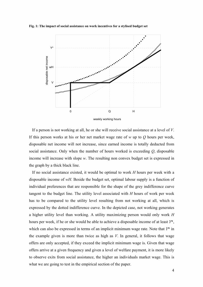
Fig. 1: The impact of social assistance on work incentives for a stylised budget set

H

V

0

wH

Y*

Q

weekly working hours

disp

osab

le n

et in

com

e

If a person is not working at all, he or she will receive social assistance at a level of V.

If this person works at his or her net market wage rate of w up to Q hours per week,

disposable net income will not increase, since earned income is totally deducted from

social assistance. Only when the number of hours worked is exceeding Q, disposable

income will increase with slope w. The resulting non convex budget set is expressed in

the graph by a thick black line.

If no social assistance existed, it would be optimal to work H hours per week with a

disposable income of wH. Beside the budget set, optimal labour supply is a function of

individual preferences that are responsible for the shape of the grey indifference curve

tangent to the budget line. The utility level associated with H hours of work per week

has to be compared to the utility level resulting from not working at all, which is

expressed by the dotted indifference curve. In the depicted case, not working generates

a higher utility level than working. A utility maximizing person would only work H

hours per week, if he or she would be able to achieve a disposable income of at least Y*,

which can also be expressed in terms of an implicit minimum wage rate. Note that Y* in

the example given is more than twice as high as V. In general, it follows that wage

offers are only accepted, if they exceed the implicit minimum wage is. Given that wage

offers arrive at a given frequency and given a level of welfare payment, it is more likely

to observe exits from social assistance, the higher an individuals market wage. This is

what we are going to test in the empirical section of the paper. 4

3 Data, Variables and Methods

This study uses data from the German Socio-Economic Panel study (GSOEP). The

yearly repeated GSOEP started 1984 in West Germany and was extended to include

East Germany in 1990. In all panel waves, the head of the household provides

information about the household and every household member aged 16 or older

provides additional individual information (for details on the GSOEP see Schupp and

Wagner 2002). Between 1992 and 2000, retrospective monthly information about social

welfare receipt for each month of the previous calendar year is part of the household

questionnaire. Excluding households with a head and if existing her partner aged 61

years or older at the beginning of the spell we observe 619 uncensored or right-censored

social welfare spells between January 1991 and December 1999, distributed on 484

households. The maximum number of spells of each household is five (one household),

379 households experience one spell of social welfare receipt (table 1). These spell data

are combined with several time-variant and time-invariant household and individual

characteristics.

Table 1 about here

In the data there are 432 uncensored and 187 right-censored observations. We are

interested in the transition from social welfare to a situation with employment income.

Therefore we differentiate between transitions to employment (187 cases) and

alternative transitions (245 cases). A transition to employment is defined as a situation

with at least one adult household member (head of the household or her partner)

working full-time subsequent to benefit receipt, at the latest beginning two month after

the spell ending.

Descriptive statistics are documented in table 2. These statistics refer (a) to the status

at the beginning of a welfare spell (n=619) and (b) to the monthly status (every month

one observation, n=8506). Spell observation mostly ends within one year (71.2%),

afterwards the number of spells ending decreases constantly. About 16% of the whole

sample end in the second year of observation, 2% in the fifth year of social assistance

receipt. These proportions refer to all spells, independent of the censor status. To

control for the economic situation we include time dummies for each year of

observation. The proportion of spells beginning in different years range from 5% in

1991 up to 15% in 1999.4 Disproportional numbers of welfare spells start in January or

5

4 One has to be careful with interpretations of these descriptive statistics. For example the increase in social assistance spells beginning in 1999 can be at least partly explained by the new sub sample F

end in December. Therefore we include January and December dummies in our

analyses. The head of a household or her partner is aged older than 50 years in 12% of

the observed spells and in 25% a foreign head or partner is living in the household.

Children aged 6 years and younger live in 39% per cent of the households, children

between 6 and 18 in 34%. In nearly all households the head or her partner has a school

graduation (94%) while only in about one third of all households at least one of these

persons has finished vocational training (32%). In every tenth household the head or his

partner is handicapped, which means that at least one of these persons answers the

question whether he or she is officially registered as having a reduced capacity for work

or of being severely disabled with yes. The statistics based on the observed months

differ from the reported statistics due to the higher weight of longer spells.

Table 2 about here

Before discussing the ratio and the difference between the potential household

income in case of one adult person working full-time and the social assistance amount,

we describe the estimating and calculating procedures of these two income sources

separately in the following.

3.1 Estimation of Potential Net-Income

In a first step we estimate potential gross market wages of all heads of the household

and as the case may be of their partner. We cannot observe their wages directly because

most of the individuals in our data set are not working while receiving social assistance.

Therefore we estimate the potential wages using all individuals in working age.

Whether or not we observe wages depends on an individual’s participation decision.

Due to this self-selection we cannot assume the sample of workers to be a random

sample of all potential working individuals and we have to account for the sample

selection problem.

The sample selection model we apply, also referred to as the type II Tobit model,

consists of a log-linear wage equation

iii Xw 111log εβ +=

with X1i as a vector containing exogenous characteristics and wi as person’s i wage and

an equation describing the binary choice to work or not to work and therefore

determining the sample selection

iii Xz 222* εβ += .

6

(Innovation Sample) of the GSOEP in 2000. Due to this new sample F the sample size of the GSOEP has increased substantially.

We observe wages according to the rule:

0 if 0 observed,not

0 if 1,*

**

≤=

>==

ii

ii

zzw

zzww

ii

iii

whereby indicates working or not working and this depends on the characteristics

X

iz

2i. Following Heckman (1979) one can estimate the wage equation consistently

assuming that the two error components of the two equations follow a bivariate normal

distribution.

We estimate two models, one for East and one for West Germany with a pooled

sample using the GSOEP waves from 1991 – 1999. The estimation results are reported

in tables 3 and 4. We control for the year and the region. As one can see, the inverse

Mills ratio term is positive and statistically significant in both models. Education,

measured in years, age and firm specific capital, measured in years being employed at

the actual employer, have significantly positive influence on the wage per hour, while

the squared age and the squared firm specific capital have a significantly negative

impact. Foreigners and women have lower wages in both regions and the absence from

the labour market in years, accounting for the previous five years, have a negative

impact on the wage. While the squared absence from the labour market influences the

wage positively in East Germany, the effect in West Germany is insignificant.

Table 3 about here

Table 4 about here

Using these estimation results, we calculate a potential monthly full-time gross wage

for each head of household and her partner. Calculating the potential net income, we

assume that in the case of a partner household the person with the higher income would

work and we account for income taxes, social security contributions and child

allowance.

3.2 Social Assistance

The amount of social assistance was not asked in all waves of the GSOEP.

Furthermore, in the years the amount of social assistance was part of the questionnaire,

the actual amount but not the monthly amount during the previous year was asked.

Therefore we can observe the monthly receipt as a binary variable but not the

corresponding amount of social assistance.

Instead of direct observation we calculate the maximum of social assistance. As

described above this amount depends on the number and the age of household members

and varies with the region and the year of receipt. We use the average yearly individual

7

basic allowances for East and West Germany to calculate the basic allowance for each

household member and add them up. Moreover we consider the one-time payments by

using the same method as Breuer and Engels (2003) or Boss (2002): We calculate 16%

of the individual basic allowance for the head of household, 17% for the partner and

20% for each child. In addition to that we take an allowance for housing depending on

the household size into account.

3.3 Ratio and Difference between Employment Income and Social Assistance

We calculate two variables: (a) The difference between the potential household net

income in case of one person working fulltime and the amount of transfer payment and

(b) the ratio of these two income sources. The nominal differences are deflated with

respect to the year 1995. We estimate different models using variables (a) or (b). The

empirical distributions of the ratio and the gap between the two income sources in the

first month of each spell are plotted in figures 2 and 3. The difference as well as the

ratio distribution indicates that the incentives to search for a job may be low for a lot of

individuals being on social welfare. Compared to the distributions of the variables

corresponding to all observed months (see appendix, figures 6 and 7), the mean of the

difference as well as of the ratio is relatively high, which reflects the higher weight of

longer spells in the distributions of all month-observations. This indicates that a lower

income ratio and income difference may go along with a longer stay in the social

assistance.

One could argue that the difference between potential household net income could

never be negative because these households would receive supplementary transfer

payments (see section 2). Nevertheless we use these negative differences in our

analysis. One can observe households who are eligible for social assistance but do non

take it up. This (non-) take-up behaviour depends among others on the expected benefit

amount (see e.g. Riphahn 2001): The probability of take-up rises with the potential

amount of transfer payments. Because we are interested in the leaving processes of

social assistance, the difference or ratio between the two separate income sources and

not the combination of the different income sources is the relevant variable.

8

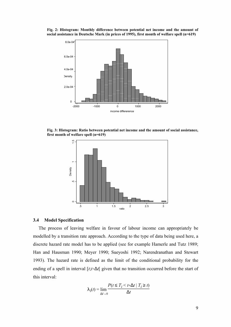
Fig. 2: Histogram: Monthly difference between potential net income and the amount of social assistance in Deutsche Mark (in prices of 1995), first month of welfare spell (n=619)

0

2.0e-04

4.0e-04

6.0e-04

8.0e-04

Density

-2000 -1000 0 1000 2000

income differerence

Fig. 3: Histogram: Ratio between potential net income and the amount of social assistance, first month of welfare spell (n=619)

0.5

11.

5D

ensi

ty

.5 1 1.5 2 2.5 3ratio

3.4 Model Specification

The process of leaving welfare in favour of labour income can appropriately be

modelled by a transition rate approach. According to the type of data being used here, a

discrete hazard rate model has to be applied (see for example Hamerle and Tutz 1989;

Han and Hausman 1990; Meyer 1990; Sueyoshi 1992; Narendranathan and Stewart

1993). The hazard rate is defined as the limit of the conditional probability for the

ending of a spell in interval [t;t+∆t[ given that no transition occurred before the start of

this interval:

λi(t) = lim∆t→0

P(t ≤ Ti < t+∆t | Ti ≥ t)∆t

9

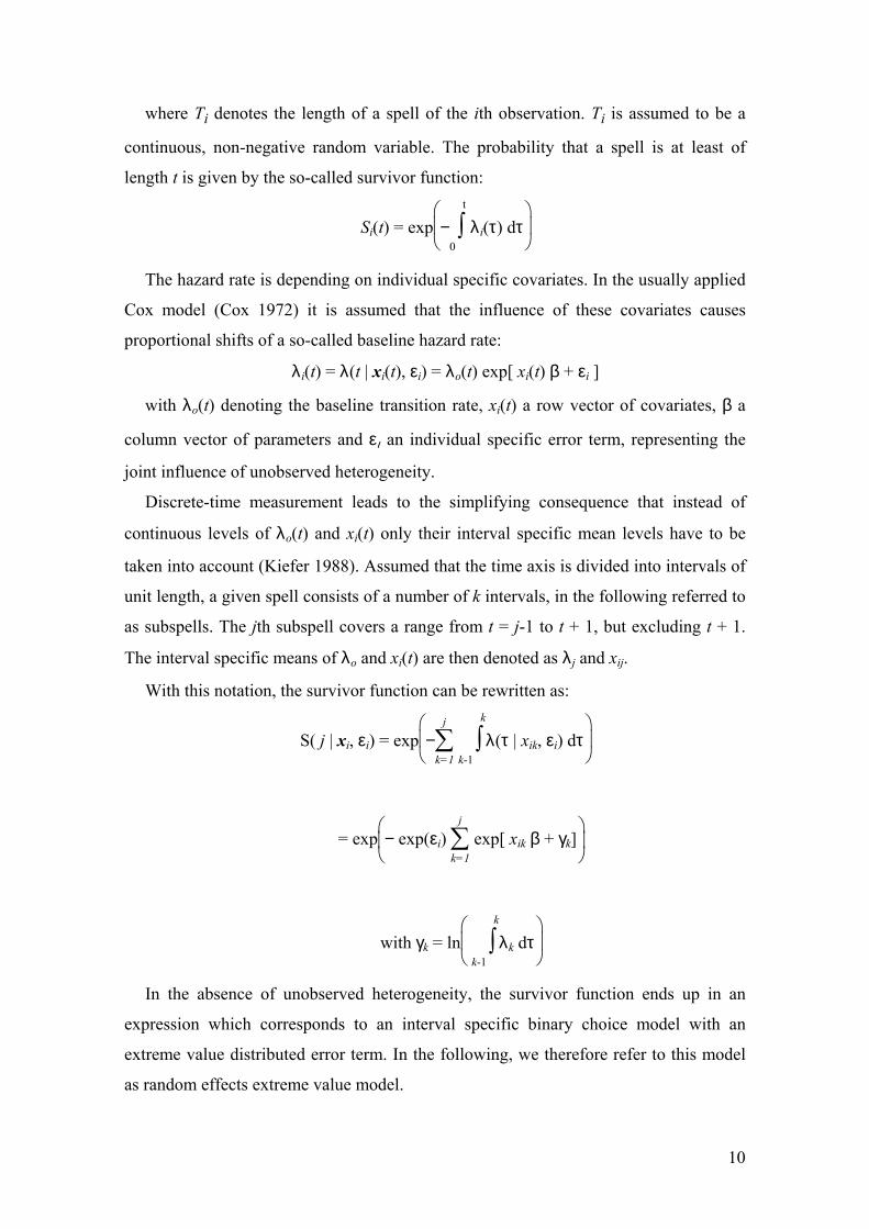
where Ti denotes the length of a spell of the ith observation. Ti is assumed to be a

continuous, non-negative random variable. The probability that a spell is at least of

length t is given by the so-called survivor function:

Si(t) = exp

−0∫

t

λi(τ) dτ

The hazard rate is depending on individual specific covariates. In the usually applied

Cox model (Cox 1972) it is assumed that the influence of these covariates causes

proportional shifts of a so-called baseline hazard rate:

λi(t) = λ(t | xi(t), εi) = λo(t) exp[ xi(t) β + εi ]

with λo(t) denoting the baseline transition rate, xi(t) a row vector of covariates, β a

column vector of parameters and ει an individual specific error term, representing the

joint influence of unobserved heterogeneity.

Discrete-time measurement leads to the simplifying consequence that instead of

continuous levels of λo(t) and xi(t) only their interval specific mean levels have to be

taken into account (Kiefer 1988). Assumed that the time axis is divided into intervals of

unit length, a given spell consists of a number of k intervals, in the following referred to

as subspells. The jth subspell covers a range from t = j-1 to t + 1, but excluding t + 1.

The interval specific means of λo and xi(t) are then denoted as λj and xij.

With this notation, the survivor function can be rewritten as:

S( j | xi, εi) = exp

−k=1∑

j

k-1∫

k

λ(τ | xik, εi) dτ

= exp

− exp(εi) k=1∑

j

exp[ xik β + γk]

with γk = ln

k-1∫

k

λk dτ

In the absence of unobserved heterogeneity, the survivor function ends up in an

expression which corresponds to an interval specific binary choice model with an

extreme value distributed error term. In the following, we therefore refer to this model

as random effects extreme value model.

10

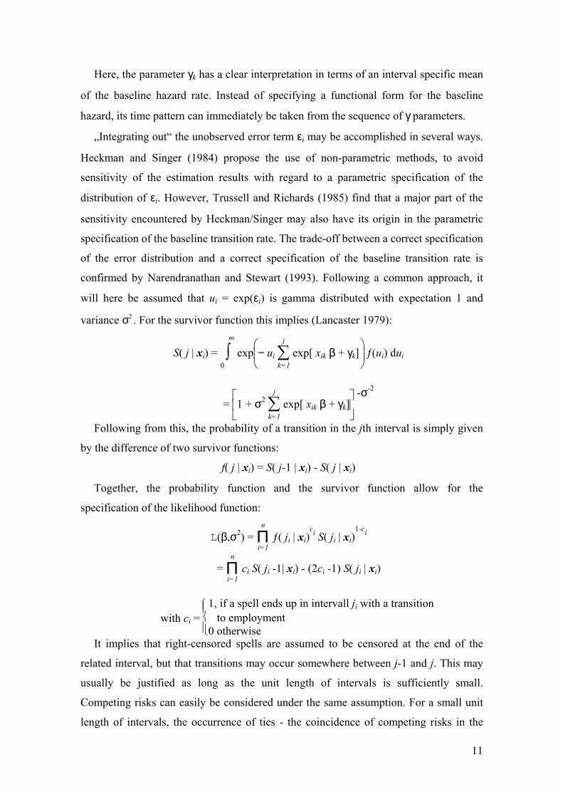
Here, the parameter γk has a clear interpretation in terms of an interval specific mean

of the baseline hazard rate. Instead of specifying a functional form for the baseline

hazard, its time pattern can immediately be taken from the sequence of γ parameters.

„Integrating out“ the unobserved error term εi may be accomplished in several ways.

Heckman and Singer (1984) propose the use of non-parametric methods, to avoid

sensitivity of the estimation results with regard to a parametric specification of the

distribution of εi. However, Trussell and Richards (1985) find that a major part of the

sensitivity encountered by Heckman/Singer may also have its origin in the parametric

specification of the baseline transition rate. The trade-off between a correct specification

of the error distribution and a correct specification of the baseline transition rate is

confirmed by Narendranathan and Stewart (1993). Following a common approach, it

will here be assumed that ui = exp(εi) is gamma distributed with expectation 1 and

variance σ . For the survivor function this implies (Lancaster 1979): 2

S( j | xi) = 0∫

∞

exp

− ui k=1∑

j

exp[ xik β + γk] ƒ(ui) dui

=

1 + σ2

k=1∑

j

exp[ xik β + γk] -σ-2

Following from this, the probability of a transition in the jth interval is simply given

by the difference of two survivor functions:

f( j | xi) = S( j-1 | xi) - S( j | xi)

Together, the probability function and the survivor function allow for the

specification of the likelihood function:

L(β,σ2) = i=1Π

n

ƒ( ji | xi)ci S( ji | xi)

1-ci

= i=1Π

n

ci S( ji -1| xi) - (2ci -1) S( ji | xi)

with ci = 1, if a spell ends up in intervall ji with a transition to employment0 otherwise

It implies that right-censored spells are assumed to be censored at the end of the

related interval, but that transitions may occur somewhere between j-1 and j. This may

usually be justified as long as the unit length of intervals is sufficiently small.

Competing risks can easily be considered under the same assumption. For a small unit

length of intervals, the occurrence of ties - the coincidence of competing risks in the

11

same interval - can be excluded. If in addition, the individual heterogeneity components

εir for different potential transitions are mutually independent, the corresponding

likelihood can be written in a factorised form. As a consequence, transitions to different

destination states can be estimated separately.

Using a cumulative parameterisation of the baseline hazard function, Han and

Hausman (1990) show that the proportional hazard specification may also be interpreted

in terms of a specific type of the ordered logit model. In practice, however, especially

for competing risks models, multinomial logit specifications are often used instead (see

e.g. Allison 1982). The multinomial logit specification does not rely on the

proportionality assumption. We also include unobserved heterogeneity in the model

which can be interpreted as random effects or random intercepts (Rabe-Hesketh et al.

2001). These random effects are assumed to be risk specific and to be constant for a

given episode. A similar approach is presented by Steiner (2001) in an analysis of

unemployment duration. We assume the unobserved heterogeneity εir to be normally

distributed with expectation 0 and variance , where r is denoting one of the two

competing risks being considered. This corresponds to a discrete hazard rate given by:

2rσ

),0(~ ,))()(exp(1

))()(exp(),)(( 2

2

1

rir

ririrr

irirririir N

txt

txttxt σε

βεα

βεαελ

∑=

+++

++= ,

whereby 1iλ indicates a transition from welfare to work and 2iλ an alternative

transition. The survivor function is given by:

∏∑

−

=

=

+++=

1

12

1

))()(exp(1

1),)((t

k

ririrr

iri

kxkkxtS

βεαε

and the likelihood function corresponds to:

irir

n

i r

t

kiriir

ciriir dfkxktxtL irt εεελελ )()],)((1[)],)(([

1

2

1

1

1∏ ∫∏ ∏

= =

−

=

−= ,

whereby cirt = 1 indicates an uncensored ending of the welfare spell in period t. The

contribution of the episode i to the sample likelihood is given by integration of the

transition probability for an uncensored and of the survivor function for a censored spell

over the random intercepts distribution5.

5 The maximum likelihood function is solved applying Gauss-Hermite quadrature using the routine gllamm (Generalized linear latent and mixed models) for Stata, developed by Rabe-Hesketh et al. (2001, 2002).

12

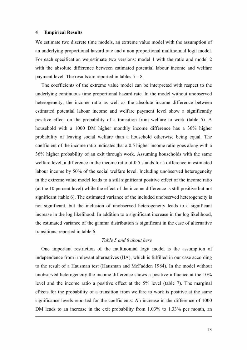
4 Empirical Results

We estimate two discrete time models, an extreme value model with the assumption of

an underlying proportional hazard rate and a non proportional multinomial logit model.

For each specification we estimate two versions: model 1 with the ratio and model 2

with the absolute difference between estimated potential labour income and welfare

payment level. The results are reported in tables 5 – 8.

The coefficients of the extreme value model can be interpreted with respect to the

underlying continuous time proportional hazard rate. In the model without unobserved

heterogeneity, the income ratio as well as the absolute income difference between

estimated potential labour income and welfare payment level show a significantly

positive effect on the probability of a transition from welfare to work (table 5). A

household with a 1000 DM higher monthly income difference has a 36% higher

probability of leaving social welfare than a household otherwise being equal. The

coefficient of the income ratio indicates that a 0.5 higher income ratio goes along with a

36% higher probability of an exit through work. Assuming households with the same

welfare level, a difference in the income ratio of 0.5 stands for a difference in estimated

labour income by 50% of the social welfare level. Including unobserved heterogeneity

in the extreme value model leads to a still significant positive effect of the income ratio

(at the 10 percent level) while the effect of the income difference is still positive but not

significant (table 6). The estimated variance of the included unobserved heterogeneity is

not significant, but the inclusion of unobserved heterogeneity leads to a significant

increase in the log likelihood. In addition to a significant increase in the log likelihood,

the estimated variance of the gamma distribution is significant in the case of alternative

transitions, reported in table 6.

Table 5 and 6 about here

One important restriction of the multinomial logit model is the assumption of

independence from irrelevant alternatives (IIA), which is fulfilled in our case according

to the result of a Hausman test (Hausman and McFadden 1984). In the model without

unobserved heterogeneity the income difference shows a positive influence at the 10%

level and the income ratio a positive effect at the 5% level (table 7). The marginal

effects for the probability of a transition from welfare to work is positive at the same

significance levels reported for the coefficients: An increase in the difference of 1000

DM leads to an increase in the exit probability from 1.03% to 1.33% per month, an

13

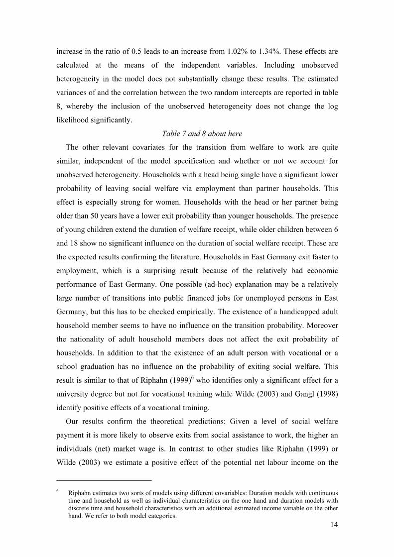
increase in the ratio of 0.5 leads to an increase from 1.02% to 1.34%. These effects are

calculated at the means of the independent variables. Including unobserved

heterogeneity in the model does not substantially change these results. The estimated

variances of and the correlation between the two random intercepts are reported in table

8, whereby the inclusion of the unobserved heterogeneity does not change the log

likelihood significantly.

Table 7 and 8 about here

The other relevant covariates for the transition from welfare to work are quite

similar, independent of the model specification and whether or not we account for

unobserved heterogeneity. Households with a head being single have a significant lower

probability of leaving social welfare via employment than partner households. This

effect is especially strong for women. Households with the head or her partner being

older than 50 years have a lower exit probability than younger households. The presence

of young children extend the duration of welfare receipt, while older children between 6

and 18 show no significant influence on the duration of social welfare receipt. These are

the expected results confirming the literature. Households in East Germany exit faster to

employment, which is a surprising result because of the relatively bad economic

performance of East Germany. One possible (ad-hoc) explanation may be a relatively

large number of transitions into public financed jobs for unemployed persons in East

Germany, but this has to be checked empirically. The existence of a handicapped adult

household member seems to have no influence on the transition probability. Moreover

the nationality of adult household members does not affect the exit probability of

households. In addition to that the existence of an adult person with vocational or a

school graduation has no influence on the probability of exiting social welfare. This

result is similar to that of Riphahn (1999)6 who identifies only a significant effect for a

university degree but not for vocational training while Wilde (2003) and Gangl (1998)

identify positive effects of a vocational training.

Our results confirm the theoretical predictions: Given a level of social welfare

payment it is more likely to observe exits from social assistance to work, the higher an

individuals (net) market wage is. In contrast to other studies like Riphahn (1999) or

Wilde (2003) we estimate a positive effect of the potential net labour income on the

14

6 Riphahn estimates two sorts of models using different covariables: Duration models with continuous time and household as well as individual characteristics on the one hand and duration models with discrete time and household characteristics with an additional estimated income variable on the other hand. We refer to both model categories.

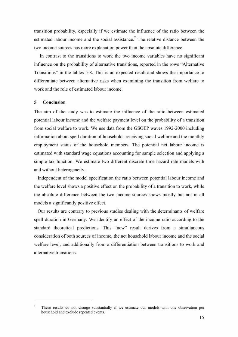
transition probability, especially if we estimate the influence of the ratio between the

estimated labour income and the social assistance.7 The relative distance between the

two income sources has more explanation power than the absolute difference.

In contrast to the transitions to work the two income variables have no significant

influence on the probability of alternative transitions, reported in the rows “Alternative

Transitions” in the tables 5-8. This is an expected result and shows the importance to

differentiate between alternative risks when examining the transition from welfare to

work and the role of estimated labour income.

5 Conclusion

The aim of the study was to estimate the influence of the ratio between estimated

potential labour income and the welfare payment level on the probability of a transition

from social welfare to work. We use data from the GSOEP waves 1992-2000 including

information about spell duration of households receiving social welfare and the monthly

employment status of the household members. The potential net labour income is

estimated with standard wage equations accounting for sample selection and applying a

simple tax function. We estimate two different discrete time hazard rate models with

and without heterogeneity.

Independent of the model specification the ratio between potential labour income and

the welfare level shows a positive effect on the probability of a transition to work, while

the absolute difference between the two income sources shows mostly but not in all

models a significantly positive effect.

Our results are contrary to previous studies dealing with the determinants of welfare

spell duration in Germany: We identify an effect of the income ratio according to the

standard theoretical predictions. This “new” result derives from a simultaneous

consideration of both sources of income, the net household labour income and the social

welfare level, and additionally from a differentiation between transitions to work and

alternative transitions.

15

7 These results do not change substantially if we estimate our models with one observation per household and exclude repeated events.

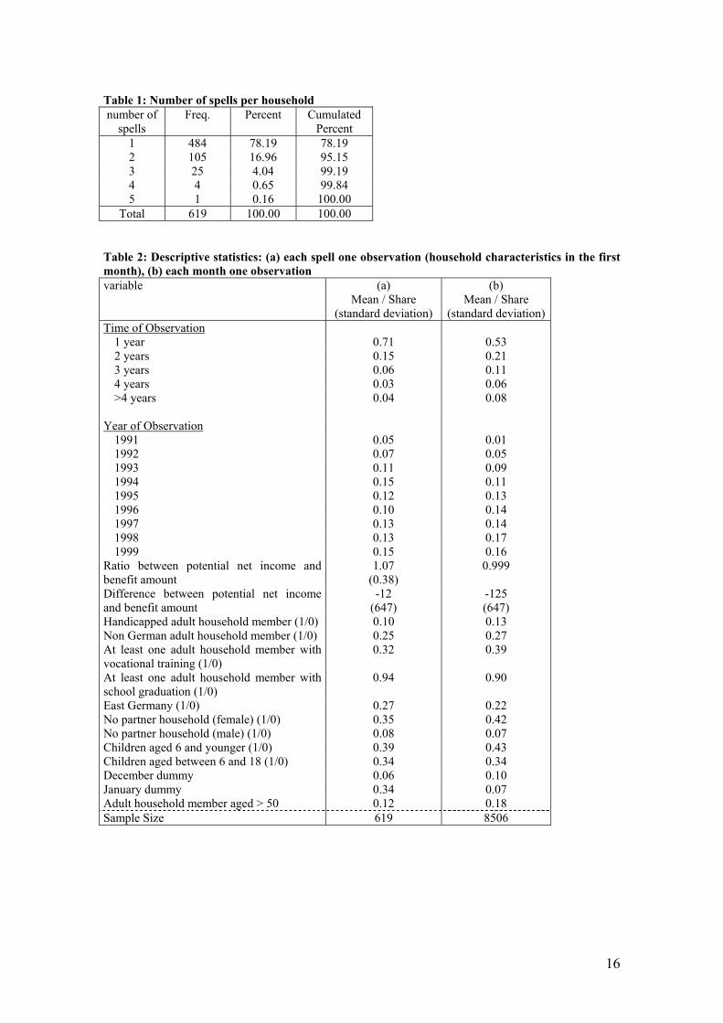
Table 1: Number of spells per household number of

spells Freq. Percent Cumulated

Percent 1 484 78.19 78.19 2 105 16.96 95.15 3 25 4.04 99.19 4 4 0.65 99.84 5 1 0.16 100.00

Total 619 100.00 100.00

Table 2: Descriptive statistics: (a) each spell one observation (household characteristics in the first month), (b) each month one observation variable (a)

Mean / Share (standard deviation)

(b) Mean / Share

(standard deviation) Time of Observation

1 year 0.71 0.53 2 years 0.15 0.21 3 years 0.06 0.11 4 years 0.03 0.06 >4 years 0.04 0.08

Year of Observation 1991 0.05 0.01 1992 0.07 0.05 1993 0.11 0.09 1994 0.15 0.11 1995 0.12 0.13 1996 0.10 0.14 1997 0.13 0.14 1998 0.13 0.17 1999 0.15 0.16

Ratio between potential net income and benefit amount

1.07 (0.38)

0.999

Difference between potential net income and benefit amount

-12 (647)

-125 (647)

Handicapped adult household member (1/0) 0.10 0.13 Non German adult household member (1/0) 0.25 0.27 At least one adult household member with vocational training (1/0)

0.32 0.39

At least one adult household member with school graduation (1/0)

0.94 0.90

East Germany (1/0) 0.27 0.22 No partner household (female) (1/0) 0.35 0.42 No partner household (male) (1/0) 0.08 0.07 Children aged 6 and younger (1/0) 0.39 0.43 Children aged between 6 and 18 (1/0) 0.34 0.34 December dummy 0.06 0.10 January dummy 0.34 0.07 Adult household member aged > 50 0.12 0.18 Sample Size 619 8506

16

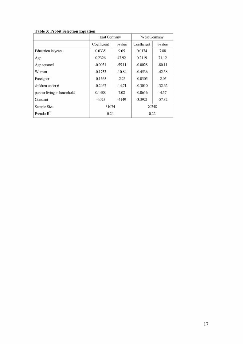
Table 3: Probit Selection Equation East Germany West Germany Coefficient t-value Coefficient t-value Education in years 0.0335 9.05 0.0174 7.88

Age 0.2326 47.92 0.2119 71.12

Age squared -0.0031 -55.11 -0.0028 -80.11

Woman -0.1753 -10.84 -0.4536 -42.38

Foreigner -0.1565 -2.25 -0.0305 -2.05

children under 6 -0.2467 -14.71 -0.3010 -32.62

partner living in household 0.1488 7.02 -0.0616 -4.57

Constant -4.075 -4149 -3.3921 -57.32

Sample Size 31074 70248

Pseudo-R2 0.24 0.22

17

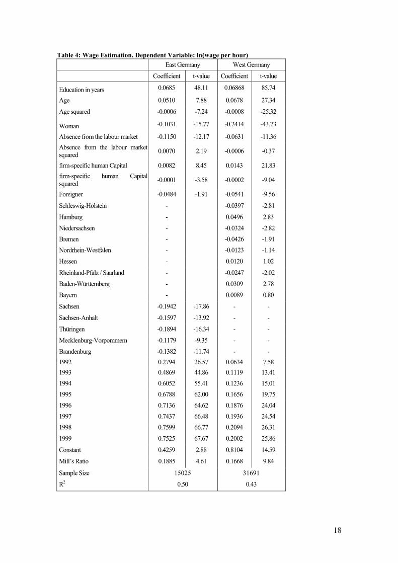
Table 4: Wage Estimation. Dependent Variable: ln(wage per hour) East Germany West Germany

Coefficient t-value Coefficient t-value

Education in years 0.0685 48.11 0.06868 85.74

Age 0.0510 7.88 0.0678 27.34

Age squared -0.0006 -7.24 -0.0008 -25.32

Woman -0.1031 -15.77 -0.2414 -43.73

Absence from the labour market -0.1150 -12.17 -0.0631 -11.36 Absence from the labour market squared 0.0070 2.19 -0.0006 -0.37

firm-specific human Capital 0.0082 8.45 0.0143 21.83 firm-specific human Capital squared -0.0001 -3.58 -0.0002 -9.04

Foreigner -0.0484 -1.91 -0.0541 -9.56

Schleswig-Holstein - -0.0397 -2.81

Hamburg - 0.0496 2.83

Niedersachsen - -0.0324 -2.82

Bremen - -0.0426 -1.91 Nordrhein-Westfalen - -0.0123 -1.14

Hessen - 0.0120 1.02

Rheinland-Pfalz / Saarland - -0.0247 -2.02

Baden-Württemberg - 0.0309 2.78

Bayern - 0.0089 0.80

Sachsen -0.1942 -17.86 - -

Sachsen-Anhalt -0.1597 -13.92 - -

Thüringen -0.1894 -16.34 - -

Mecklenburg-Vorpommern -0.1179 -9.35 - -

Brandenburg -0.1382 -11.74 - - 1992 0.2794 26.57 0.0634 7.58 1993 0.4869 44.86 0.1119 13.41 1994 0.6052 55.41 0.1236 15.01 1995 0.6788 62.00 0.1656 19.75

1996 0.7136 64.62 0.1876 24.04 1997 0.7437 66.48 0.1936 24.54 1998 0.7599 66.77 0.2094 26.31

1999 0.7525 67.67 0.2002 25.86

Constant 0.4259 2.88 0.8104 14.59

Mill’s Ratio 0.1885 4.61 0.1668 9.84

Sample Size 15025 31691

R2 0.50 0.43

18

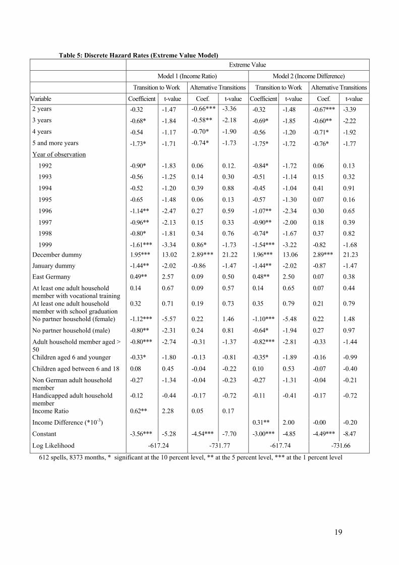
Table 5: Discrete Hazard Rates (Extreme Value Model) Extreme Value

Model 1 (Income Ratio) Model 2 (Income Difference)

Transition to Work Alternative Transitions Transition to Work Alternative Transitions

Variable Coefficient t-value Coef. t-value Coefficient t-value Coef. t-value 2 years -0.32 -1.47 -0.66*** -3.36 -0.32 -1.48 -0.67*** -3.39 3 years -0.68* -1.84 -0.58** -2.18 -0.69* -1.85 -0.60** -2.22 4 years -0.54 -1.17 -0.70* -1.90 -0.56 -1.20 -0.71* -1.92 5 and more years -1.73* -1.71 -0.74* -1.73 -1.75* -1.72 -0.76* -1.77 Year of observation

1992 -0.90* -1.83 0.06 0.12. -0.84* -1.72 0.06 0.13 1993 -0.56 -1.25 0.14 0.30 -0.51 -1.14 0.15 0.32

1994 -0.52 -1.20 0.39 0.88 -0.45 -1.04 0.41 0.91

1995 -0.65 -1.48 0.06 0.13 -0.57 -1.30 0.07 0.16

1996 -1.14** -2.47 0.27 0.59 -1.07** -2.34 0.30 0.65

1997 -0.96** -2.13 0.15 0.33 -0.90** -2.00 0.18 0.39 1998 -0.80* -1.81 0.34 0.76 -0.74* -1.67 0.37 0.82

1999 -1.61*** -3.34 0.86* -1.73 -1.54*** -3.22 -0.82 -1.68 December dummy 1.95*** 13.02 2.89*** 21.22 1.96*** 13.06 2.89*** 21.23 January dummy -1.44** -2.02 -0.86 -1.47 -1.44** -2.02 -0.87 -1.47 East Germany 0.49** 2.57 0.09 0.50 0.48** 2.50 0.07 0.38

At least one adult household member with vocational training

0.14 0.67 0.09 0.57 0.14 0.65 0.07 0.44

At least one adult household member with school graduation

0.32 0.71 0.19 0.73 0.35 0.79 0.21 0.79

No partner household (female) -1.12*** -5.57 0.22 1.46 -1.10*** -5.48 0.22 1.48

No partner household (male) -0.80** -2.31 0.24 0.81 -0.64* -1.94 0.27 0.97

Adult household member aged > 50

-0.80*** -2.74 -0.31 -1.37 -0.82*** -2.81 -0.33 -1.44

Children aged 6 and younger -0.33* -1.80 -0.13 -0.81 -0.35* -1.89 -0.16 -0.99

Children aged between 6 and 18 0.08 0.45 -0.04 -0.22 0.10 0.53 -0.07 -0.40

Non German adult household member

-0.27 -1.34 -0.04 -0.23 -0.27 -1.31 -0.04 -0.21

Handicapped adult household member

-0.12 -0.44 -0.17 -0.72 -0.11 -0.41 -0.17 -0.72

Income Ratio 0.62** 2.28 0.05 0.17

Income Difference (*10-3) 0.31** 2.00 -0.00 -0.20

Constant -3.56*** -5.28 -4.54*** -7.70 -3.00*** -4.85 -4.49*** -8.47

Log Likelihood -617.24 -731.77 -617.74 -731.66

612 spells, 8373 months, * significant at the 10 percent level, ** at the 5 percent level, *** at the 1 percent level

19

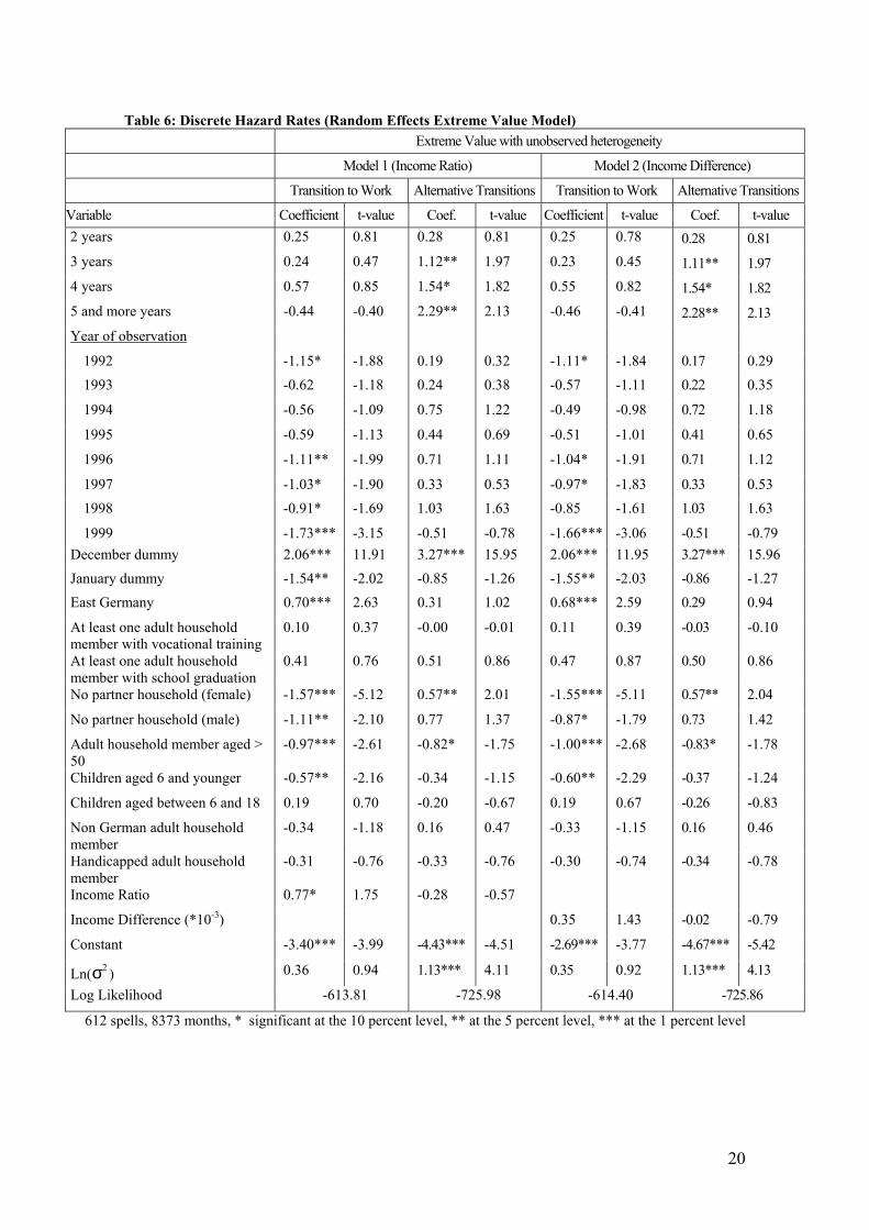
Table 6: Discrete Hazard Rates (Random Effects Extreme Value Model) Extreme Value with unobserved heterogeneity



Variable Coefficient t-value Coef. t-value Coefficient t-value Coef. t-value 2 years 0.25 0.81 0.28 0.81 0.25 0.78 0.28 0.81 3 years 0.24 0.47 1.12** 1.97 0.23 0.45 1.11** 1.97 4 years 0.57 0.85 1.54* 1.82 0.55 0.82 1.54* 1.82 5 and more years -0.44 -0.40 2.29** 2.13 -0.46 -0.41 2.28** 2.13 Year of observation

1992 -1.15* -1.88 0.19 0.32 -1.11* -1.84 0.17 0.29 1993 -0.62 -1.18 0.24 0.38 -0.57 -1.11 0.22 0.35

1994 -0.56 -1.09 0.75 1.22 -0.49 -0.98 0.72 1.18

1995 -0.59 -1.13 0.44 0.69 -0.51 -1.01 0.41 0.65

1996 -1.11** -1.99 0.71 1.11 -1.04* -1.91 0.71 1.12

1997 -1.03* -1.90 0.33 0.53 -0.97* -1.83 0.33 0.53 1998 -0.91* -1.69 1.03 1.63 -0.85 -1.61 1.03 1.63

1999 -1.73*** -3.15 -0.51 -0.78 -1.66*** -3.06 -0.51 -0.79 December dummy 2.06*** 11.91 3.27*** 15.95 2.06*** 11.95 3.27*** 15.96 January dummy -1.54** -2.02 -0.85 -1.26 -1.55** -2.03 -0.86 -1.27 East Germany 0.70*** 2.63 0.31 1.02 0.68*** 2.59 0.29 0.94

At least one adult household member with vocational training

0.10 0.37 -0.00 -0.01 0.11 0.39 -0.03 -0.10


0.41 0.76 0.51 0.86 0.47 0.87 0.50 0.86

No partner household (female) -1.57*** -5.12 0.57** 2.01 -1.55*** -5.11 0.57** 2.04



-0.97*** -2.61 -0.82* -1.75 -1.00*** -2.68 -0.83* -1.78

Children aged 6 and younger -0.57** -2.16 -0.34 -1.15 -0.60** -2.29 -0.37 -1.24



-0.34 -1.18 0.16 0.47 -0.33 -1.15 0.16 0.46


-0.31 -0.76 -0.33 -0.76 -0.30 -0.74 -0.34 -0.78

Income Ratio 0.77* 1.75 -0.28 -0.57

Income Difference (*10-3) 0.35 1.43 -0.02 -0.79

Constant -3.40*** -3.99 -4.43*** -4.51 -2.69*** -3.77 -4.67*** -5.42

Ln(σ ) 2 0.36 0.94 1.13*** 4.11 0.35 0.92 1.13*** 4.13

Log Likelihood -613.81 -725.98 -614.40 -725.86


20

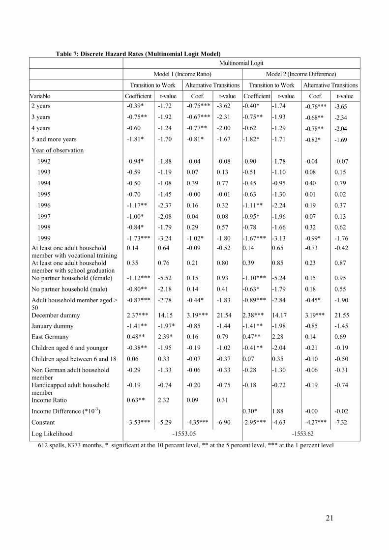
Table 7: Discrete Hazard Rates (Multinomial Logit Model) Multinomial Logit



Variable Coefficient t-value Coef. t-value Coefficient t-value Coef. t-value 2 years -0.39* -1.72 -0.75*** -3.62 -0.40* -1.74 -0.76*** -3.65 3 years -0.75** -1.92 -0.67*** -2.31 -0.75** -1.93 -0.68** -2.34 4 years -0.60 -1.24 -0.77** -2.00 -0.62 -1.29 -0.78** -2.04 5 and more years -1.81* -1.70 -0.81* -1.67 -1.82* -1.71 -0.82* -1.69 Year of observation

1992 -0.94* -1.88 -0.04 -0.08 -0.90 -1.78 -0.04 -0.07 1993 -0.59 -1.19 0.07 0.13 -0.51 -1.10 0.08 0.15

1994 -0.50 -1.08 0.39 0.77 -0.45 -0.95 0.40 0.79

1995 -0.70 -1.45 -0.00 -0.01 -0.63 -1.30 0.01 0.02

1996 -1.17** -2.37 0.16 0.32 -1.11** -2.24 0.19 0.37

1997 -1.00* -2.08 0.04 0.08 -0.95* -1.96 0.07 0.13 1998 -0.84* -1.79 0.29 0.57 -0.78 -1.66 0.32 0.62

1999 -1.73*** -3.24 -1.02* -1.80 -1.67*** -3.13 -0.99* -1.76 At least one adult household member with vocational training

0.14 0.64 -0.09 -0.52 0.14 0.65 -0.73 -0.42


0.35 0.76 0.21 0.80 0.39 0.85 0.23 0.87

No partner household (female) -1.12*** -5.52 0.15 0.93 -1.10*** -5.24 0.15 0.95



-0.87*** -2.78 -0.44* -1.83 -0.89*** -2.84 -0.45* -1.90

December dummy 2.37*** 14.15 3.19*** 21.54 2.38*** 14.17 3.19*** 21.55

January dummy -1.41** -1.97* -0.85 -1.44 -1.41** -1.98 -0.85 -1.45 East Germany 0.48** 2.39* 0.16 0.79 0.47** 2.28 0.14 0.69

Children aged 6 and younger -0.38** -1.95 -0.19 -1.02 -0.41** -2.04 -0.21 -0.19



-0.29 -1.33 -0.06 -0.33 -0.28 -1.30 -0.06 -0.31


-0.19 -0.74 -0.20 -0.75 -0.18 -0.72 -0.19 -0.74

Income Ratio 0.63** 2.32 0.09 0.31

Income Difference (*10-3) 0.30* 1.88 -0.00 -0.02

Constant -3.53*** -5.29 -4.35*** -6.90 -2.95*** -4.63 -4.27*** -7.32

Log Likelihood -1553.05 -1553.62


21

Table 8: Discrete Hazard Rates (Multinomial Logit Model with random intercepts) Multinomial Logit with unobserved heterogeneity



Variable Coefficient t-value Coef. t-value Coefficient t-value Coef. t-value 2 years -0.36 -1.28 -0.60** -2.00 -0.37 -1.29 -0.60 -2.01

3 years -0.70 -1.50 -0.37 -0.82 -0.70 -1.50 -0.37 -0.82

4 years -0.56 -0.95 -0.40 -0.67 -0.57 -0.97 -0.40 -0.67

5 and more years -1.78 -1.61 -0.29 -0.40 -1.78 -1.62 -0.30 -0.40 Year of observation

1992 -0.99* -1.79 -0.02 -0.04 -0.95 -1.73 -0.03 -0.04 1993 -0.61 -1.22 0.07 0.12 -0.57 -1.14 0.07 0.12

1994 -0.56 -1.14 0.47 0.83 -0.51 -1.02 0.47 0.84

1995 -0.74 -1.48 0.07 0.12 -0.68 -1.35 0.07 0.12

1996 -1.20** -2.32 0.26 0.44 -1.14 -2.22 0.27 0.47

1997 -1.04** -2.05 0.07 0.12 -1.00 -1.96 0.08 0.14 1998 -0.91* -1.78 0.42 0.71 -0.85 -1.68 0.43 0.74

1999 -1.78*** -3.31 -0.98 -1.61 -1.72 -3.21 -0.96 -1.60 At least one adult household member with vocational training

0.13 0.57 -0.09 -0.46 0.14 0.60 -0.08 -0.37


0.33 0.70 0.29 0.82 0.37 0.80 0.30 0.86

No partner household (female) -1.19*** -4.40 0.27 1.08 -1.17 -4.32 0.26 1.07

No partner household (male) -0.87** -2.13 0.30 0.71 -0.68 -1.79 0.32 0.82


-0.90** -2.80 -0.54* -1.74 -0.92 -2.88 -0.56 -1.79

December dummy 2.37*** 13.32 3.32*** 15.25 2.38 13.32 3.33 15.30

January dummy -1.42** -1.98 -0.82 -1.37 -1.42 -1.98 -0.82 -1.38 East Germany 0.49** 2.26 0.18 0.78 0.47 2.18 0.17 0.70

Children aged 6 and younger -0.41* -1.93 -0.21 -0.95 -0.44 -2.05 -0.23 -1.09



-0.31 -1.36 -0.02 -0.07 -0.30 -1.32 -0.01 -0.06


-0.22 -0.73 -0.22 -0.70 -0.21 -0.71 -0.22 -0.71

Income Ratio 0.64** 2.05 0.02 0.07

Income Difference (*10-3) 0.30* 1.73 -0.04 -0.19

Constant -3.65*** -4.93 -4.71*** -5.71 -3.06*** -4.43 -4.69 -5.69

σ2 0.18 0.73 0.17 0.73

ρ -0.56 -0.18

Log Likelihood -1552.56 -1553.12


22

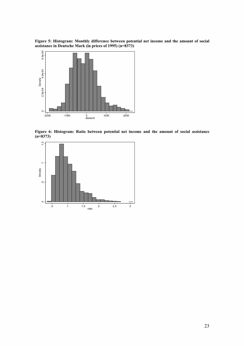
Figure 5: Histogram: Monthly difference between potential net income and the amount of social assistance in Deutsche Mark (in prices of 1995) (n=8373)

02.

0e-0

44.

0e-0

46.

0e-0

4D

ensi

ty

-2000 -1000 0 1000 2000abstand

Figure 6: Histogram: Ratio between potential net income and the amount of social assistance (n=8373)

0.5

11.

5D

ensi

ty

.5 1 1.5 2 2.5 3ratio

23

References

Blank, Rebecca M. (1989): Analyzing the Length of Welfare Spells, Journal of Public Economics, 39, 245-273.

Boss, Alfred (2002): Sozialhilfe, Lohnabstand und Leistungsanreize. Empirische Analyse für Haushaltstypen und Branchen in West- und Ostdeutschland. Kieler Studien 318. Berlin

Blundell, Richard and Thomas MaCurdy (1999), Labor Supply: A Review of Alternative Approaches. In: Orley Ashenfelter und David Card (Hrsg.), Handbook of Labor Economics, Vol. 3A. Amsterdam, 1559-1591.

Breuer, Wilhelm and Dietrich Engels (2003): Grundinformationen und Daten zur Sozialhilfe. Im Auftrag des Bundesministeriums für Gesundheit und Soziale Sicherung.

Cox, D. R. (1972), Regression Models and Life Tables“, Journal of the Royal Statistical Society Series B, 34, 187-202.

Engels, Dietrich (2001): Abstand zwischen Sozialhilfe und unteren Arbeitnehmereinkommen: Neue Ergebnisse zu einer alten Kontroverse, Sozialer Forschritt, 50, 56-62.

Gangl, Markus (1998): Sozialhilfebezug und Arbeitsmarktverhalten. Eine Längsschnittanalyse der Übergänge aus der Sozialhilfe in den Arbeitsmarkt, Zeitschrift für Soziologie, 27, 212-232.

Gittleman, Maury (2001): Declining Caseloads: What Do the Dynamics of Welfare Participation Reveal? Industrial Relations, 40, 537-570.

Hamerle, Alfred, and Gerhard Tutz (1989), Diskrete Modelle zur Analyse von Verweildauern, Frankfurt/Main, Campus.

Han, Aaron, and Jerry A. Hausman (1990), Flexible Parametric Estimation of Duration and Competing Risk Models, Journal of Applied Econometrics, 5, 1-28.

Hausman, Jerry and Daniel McFadden (1984): Specification Test for Multinomial Logit Model, Econometrica, 52, 1219-1240.

Heckman, James J. (1979): Sample Selection Bias as a Specification Error, Econometrica, 47, 153-162.

Heckman, James J., and Burton Singer (1984), Econometric Duration Analysis, Journal of Econometrics, 24, 63-132.

Kiefer, Nicholas (1987), Analysis of Grouped Duration Data. In: Statistical Inference from Stochastic Processes, edited by N. U. Prabhu. Providence, RI: American Mathematical Society, 107-137.

Lancaster, Tony (1979) Econometric Models for the Duration of Unemployment, Econometrica, 47, 939-956.

Meyer, Bruce D. (1990), Unemployment Insurance and Unemployment Spells, Econometrica, 58, 757-782.

Moffitt, Robert (1992): Incentive Effects of the U.S. Welfare System: A Review, Journal of Economic Literature, 30, 1-61.

24

25

Narendranathan, Wiji, and M.B. Stewart, How Does the Benefit Effect Vary as Unemployment Spells Lengthen?, Journal of Applied Econometrics, 8, 361-381.

Ochel, Wolfgang (2003): Welfare to Work in the U.S.: A Model for Germany? Finanzarchiv, 59, 91-119.

Rabe-Hesketh, Sophia, Andrew Pickels and Anders Skrondal (2001): GLLAMM Manual, Technical Report, Department of Biostatistics and Computing Institute of Psychiatry, Kings`s College, London.

Rabe-Hesketh, Sophia, Anders Skrondal and Andrew Pickels (2002): Reliable Estimation of generalised linear mixed models using adaptive quadrature. The Stata Journal, 2, 1-21.

Riphahn, Regina T. (1999): Why Did Social Assistance Dependence Increase? - The Dynamics of Social Assistance Dependence and Unemployment in Germany, 1999, unpublished Habilitationsschrift , University of Munich.

Riphahn, Regina T. (2001): Rational Poverty or Poor Rationality? The Take-up of Social Assistance Benefits, Review of Income and Wealth, 47, 379-398.

Schupp, Jürgen and Gert G. Wagner (2002): Maintenance of and innovation in long term panel studies: The case of the German Socio-Economic Panel (GSOEP), Allgemeines Statistisches Archiv, 86, 163-175.

Steiner, Viktor (2001): Unemployment Persistence in the West German Labour Market: Negative Duration Dependence or Sorting? Oxford Bulletin of Economics and Statistics, 63, 91-113.

Stewart, Jennifer and Martin D. Dooley (1999): The Duration of Spells On Welfare and Off Welfare among Lone Mothers in Ontario, Canadian Public Policy, 25 Supplement 1, S47-S72.

Sueyoshi, Glenn T. (1992), Semiparametric Proportional Hazards Estimation of Competing Risks Models With Time-Varying Covariates, Journal of Econometrics, 51, 25-28.

Trussell, James, and Tony Richards (1985): Correcting for Unmeasured Heterogeneity in Hazards Models Using the Heckman-Singer Procedure. In: Sociological Methodology 1985, edited by Nancy Brandon Tuma. San Francisco: Jossey-Bass, 242-276.

Voges, Jürgen and Götz Rohwer (1992): Receiving Social Assistance in Germany: Risk and Duration, Journal of European Social Policy, 2, 175-191.

Wilde, Joachim (2003): Why do Recipients of German Social Assistance Opt Out? An Empirical Investigation of Incentives with the Low Income Panel. Jahrbücher für Nationalökonomie und Statistik, 223, 719-742.

the transition from welfare to work and the role of ... · the transition from welfare to work and...

Documents