The unequal economic consequences ofcarbon pricing*

Link to most recent version

Diego R. Känzig†

London Business School

December, 2021

Abstract

This paper studies how carbon pricing affects emissions, economic aggre-

gates and inequality. Exploiting institutional features of the European car-

bon market and high-frequency data, I identify a carbon policy shock. I

find that a tighter carbon pricing regime leads to a significant increase in

energy prices, a persistent fall in emissions and an uptick in green innova-

tion. This comes at the cost of a temporary fall in economic activity, which

is not borne equally across society: poorer households lower their consump-

tion significantly while richer households are less affected. Not only are the

poor more exposed because of their higher energy share, they also experience

a larger fall in their income. These indirect effects account for over 80 per-

cent of the aggregate effect on consumption. A climate-economy model with

heterogeneity in households’ energy shares, income incidence and marginal

propensities to consume is able to account for these facts.

JEL classification: E32, E62, H23, Q54, Q58

Keywords: Carbon pricing, cap and trade, emissions, macroeconomic effects,

inequality, high-frequency identification

*I am indebted to my advisors Paolo Surico, Hélène Rey, Florin Bilbiie and João Cocco, as wellas Joseba Martinez, Elias Papaioannou, Lucrezia Reichlin, Andrew Scott and Vania Stavrakevafor their invaluable guidance and support. For helpful comments and suggestions, I thank UfukAkcigit, Asger Andersen, Michele Andreolli, Juan Antolin-Diaz, Adrien Auclert, Sandra Batten,Christiane Baumeister, Jean-Pierre Benoît, Philippe Benoît, Martin Bodenstein, Kirill Borusyak,Thomas Bourany, Jeff Campbell, James Cloyne, Joel David, Thomas Drechsel, Martin Ellison, LuisFonseca, Luca Fornaro, Claudia Foroni, Lukas Freund, Stephie Fried, Jordi Galí, Simon Gilchrist,Mike Golosov, Lars Hansen, Arshia Hashemi, Garth Heutel, Matthias Hoelzlein, Kilian Huber,Niko Jaakkola, Joe Kaboski, Greg Kaplan, Ryan Kellogg, Maral Kichian, Ralph Koijen, Max Kon-radt, Sylvain Leduc, Yueran Ma, Matthias Meier, Leo Melosi, Marti Mestieri, Stephen Millard,Silvia Miranda-Agrippino, Eric Sims, Amir Sufi, Nelson Mark, Johan Moen, Ishan Nath, TsvetiNenova, Luca Neri, Pascal Noel, Conny Olovsson, Aleks Oskolkov, Guillermo Ordoñez, ChristinaPatterson, Gert Peersman, Ivan Petrella, Michele Piffer, Richard Portes, Giorgio Primiceri, BenPugsley, Sebastian Rast, Natalie Rickard, Esteban Rossi-Hansberg, Livio Stracca, Martin Stuer-mer, Greg Upton, Rob Vigfusson, Michael Weber, Beatrice Weder di Mauro, Nicolas Werquin,Nadia Zhuravleva, Nathan Zorzi as well as participants at numerous seminars and conferences.I thank the ECB for the Young Economists’ Prize, the IAEE for the Best Student Paper Award andthe AQR Institute for the Fellowship Award. I am grateful to the Wheeler Institute for Businessand Development for generously supporting this research.

†Contact: Diego R. Känzig, London Business School, Regent’s Park, London NW1 4SA, UnitedKingdom. E-mail: dkaenzig@london.edu. Web: diegokaenzig.com.

1

1. Introduction

The looming climate crisis has put climate change at the top of the global pol-icy agenda. Governments around the world have started to implement carbonpricing policies to mitigate climate change, either via carbon taxes or cap andtrade systems. Yet, little is known about the effects of such policies in practice.Is carbon pricing effective at reducing emissions? What is the impact on output,employment, and inflation and who bears the economic costs of these policies?

This paper seeks to answer all these questions. I propose a novel approach toidentify the aggregate and distributional effects of carbon pricing, exploiting in-stitutional features of the European carbon market and high-frequency data. TheEuropean Union Emissions Trading System (EU ETS) is the largest and oldestcarbon market in the world, covering around 40 percent of the EU’s greenhousegas (GHG) emissions. The market was established in phases and the regulationshave been updated continuously. Following an event study approach, I collected113 regulatory update events concerning the supply of emission allowances. Bymeasuring the change in the carbon futures price in a tight window around theregulatory news, I isolate a series of carbon policy surprises. Reverse causalitycan be plausibly ruled out as economic conditions are known and priced by themarket prior to the regulatory news and unlikely to change within the tight win-dow. Using the surprise series as an instrument, I estimate the dynamic causaleffects of a carbon policy shock.

I find that carbon pricing has significant effects on emissions and the economy.A carbon policy shock tightening the carbon pricing regime causes a strong, im-mediate increase in energy prices and a persistent fall in overall GHG emissions.Thus, carbon pricing is successful in achieving its goal of reducing emissions.However, this does not come without a cost. Consumer prices rise significantlyand economic activity falls, as reflected in lower output and higher unemploy-ment. Crucially, the fall in activity is somewhat less persistent than the fall inemissions – improving the emissions intensity in the longer term. The stock mar-ket falls for about one and a half years but then rebounds and turns positiveafter. The euro depreciates in real terms and imports fall significantly. Whilethe shock leads to somewhat heightened financial uncertainty and a short-termdeterioration of financial conditions, the main transmission channel appears towork through higher carbon prices, which passing through energy prices leadsto lower consumption and investment. At the same time, carbon pricing cre-ates an incentive for green innovation, causing a significant uptick in low-carbonpatenting.

2

Carbon policy shocks have also contributed meaningfully to historical vari-ations in prices, emissions and macroeconomic aggregates. However, they didnot account for the fall in emissions associated with the global financial crisis –supporting the validity of the identified shock.

My results illustrate a trade-off between reducing emissions and the eco-nomic costs of climate change mitigation policies. Importantly, these costs arenot equally distributed across society. Using detailed household-level data, Idocument pervasive heterogeneity in the expenditure response to carbon pol-icy shocks. While the expenditure of higher-income households only fallsmarginally, low-income households reduce their expenditure significantly andpersistently. These households are more severely affected in two ways. First, theyspend a larger share of their disposable income on energy and thus the higher en-ergy bill leaves significantly fewer resources for other expenditures. Second, theyexperience a stronger fall in income, as they tend to work in sectors that are moreimpacted by the policy. Interestingly, these are not the sectors with the highestenergy intensity but sectors that are more sensitive to changes in demand, pro-ducing more discretionary goods and services. Crucially, the magnitudes of theexpenditure responses are much larger than what can be accounted for by thedirect effect through energy prices alone. This points to an important role of in-direct, general equilibrium effects via income and employment. My estimatessuggest that indirect effects account for over 80 percent of the aggregate effect onconsumption, while direct effects account for less than 20 percent.

My findings on the distributional impact suggest that targeted fiscal policiescould be an effective way to reduce the economic costs of carbon pricing. Tothe extent that energy demand is inelastic, which turns out to be the case espe-cially for poorer households, this should not compromise emission reductions.This intuition is confirmed in a climate-economy model with nominal rigiditiesand heterogeneity in households’ energy expenditure shares, income incidenceand marginal propensities to consume (MPCs). The model can account for theobserved empirical responses to carbon policy, both in terms of absolute magni-tudes and relative importance of direct and indirect effects. Based on this model,I show that redistributing carbon revenues can mitigate the fall in aggregate con-sumption and reduce the regressive distributional consequences of carbon pric-ing, without compromising emission reductions. Finally, I provide some sugges-tive evidence that carbon pricing leads to a fall in the support for climate-relatedpolicies that is particularly pronounced among low-income households. Thus,such targeted compensation may also help to increase the public support for cli-mate policy.

3

A comprehensive series of sensitivity checks indicate that the results are ro-bust along a number of other dimensions including the selection of event dates,the estimation technique, the model specification, and the sample period. Impor-tantly, the results are also robust to accounting for confounding news over theevent window using an heteroskedasticity-based estimator.

Related literature and contribution. This paper contributes to a growing litera-ture studying the effects of climate policy and carbon pricing in particular. Whilethere is mounting evidence on the effectiveness of such policies for emission re-ductions (Martin, De Preux, and Wagner, 2014; Andersson, 2019, among others),less is known about the economic effects. A number of studies have analyzed themacroeconomic effects of the British Columbia carbon tax, finding no significantimpacts on GDP (Metcalf, 2019; Bernard and Kichian, 2021). Metcalf and Stock(2020a,b) study the macroeconomic impacts of carbon taxes in European coun-tries. They find no robust evidence of a negative effect of the tax on employmentor GDP growth.1 In a similar vein, Konradt and di Mauro (2021) find that car-bon taxes in Europe and Canada do not appear to be inflationary. In contrast,theoretical studies based on computable general equilibrium models tend to findcontractionary output effects (see e.g. McKibbin et al., 2017; Goulder and Haf-stead, 2018). I contribute to this literature by providing new estimates based onthe EU ETS, the largest carbon market in the world.

A large literature has studied the macroeconomic effects of discretionary taxchanges more generally. To address the endogeneity of tax changes, the literaturehas used SVAR techniques (Blanchard and Perotti, 2002) and narrative methods(Romer and Romer, 2010). The narrative approach in particular points to largemacroeconomic effects; a tax increase leads to a significant and persistent declineof output and its components (see also Mertens and Ravn, 2013; Cloyne, 2013).However, it is unclear how much we can learn from these estimates with respectto carbon pricing, which is enacted to correct a clear externality and not becauseof past decisions or ideology. While the motivation behind carbon pricing is ar-guably long-term and thus more likely unrelated to the current state of the econ-omy – similar to the tax changes considered in Romer and Romer (2010) – it is stillperceivable that regulatory decisions also take economic conditions into account.

To address this potential endogeneity in carbon pricing, I propose a novelidentification strategy exploiting high-frequency variation. From a methodologi-cal viewpoint, my approach is closely related to the literature on high-frequency

1Contrary to this paper, Metcalf and Stock (2020a,b) do not study the effects of the EU ETS butnational carbon taxes, which are present in many European countries and cover sectors that arenot included in the EU ETS.

4

identification, which was developed in the monetary policy setting (Kuttner,2001; Gürkaynak, Sack, and Swanson, 2005; Gertler and Karadi, 2015; Nakamuraand Steinsson, 2018, among others) and more recently employed in the globaloil market context (Känzig, 2021). In this literature, policy surprises are identi-fied using high-frequency asset price movements around policy events, such asFOMC or OPEC meetings. The idea is to isolate the impact of policy news bymeasuring the change in asset prices in a tight window around the events.

I contribute to this literature by extending the high-frequency identificationapproach to climate policy, exploiting institutional features of the European car-bon market. A number of studies have used event study techniques to analyzethe effects of regulatory news on carbon, energy and stock prices (Mansanet-Bataller and Pardo, 2009; Fan et al., 2017; Bushnell, Chong, and Mansur, 2013,among others). To the best of my knowledge, however, this paper is the first toexploit these regulatory updates to analyze the economic effects of carbon pric-ing. The approach is very general and could also be employed to evaluate theperformance of other cap and trade systems.

Equipped with this novel identification strategy, I provide new evidence notonly on the aggregate but also on the distributional consequences of carbon pric-ing. There is growing consensus that the transition to a low-carbon economy hasto be fair and equitable (see e.g. European Comission, 2021). Therefore, it is cru-cial to understand how carbon pricing affects economic inequality. I find that car-bon pricing in the EU has been more regressive than commonly thought, burden-ing lower-income households substantially more than richer ones. This stands incontrast to existing studies, which tend to find a more modest regressive impact(Beznoska, Cludius, and Steiner, 2012; Ohlendorf et al., 2021). My findings il-lustrate the importance of accounting for indirect, general-equilibrium effects viaincome and employment; solely focusing on the direct effects via higher energyprices can massively understate the actual distributional impact.

Finally, I show that the distributional consequences do not only matter for in-equality but also for the transmission of the policy to the macroeconomy. Myresults are consistent with models where unequal income incidence linked toheterogeneous MPCs can lead to a powerful amplification of aggregate demandfluctuations (Bilbiie, 2008; Auclert, 2019; Patterson, 2021). Building on this litera-ture, I develop a new climate-economy economy model (in spirit of Heutel, 2012;Golosov et al., 2014; Annicchiarico and Di Dio, 2015) with heterogeneity in house-holds’ energy shares, income incidence, and MPCs and show that such a modelcan account for the empirical facts. In this sense, I also contribute to an influentialliterature studying the role of heterogeneity in the transmission of fiscal policies

5

(see e.g. Johnson, Parker, and Souleles, 2006; Kaplan and Violante, 2014; Cloyneand Surico, 2017, among many others).

More generally, my results illustrate that carbon-policy induced changes inenergy prices transmit through a powerful demand channel that can outweighthe traditional cost channel by an order of magnitude. This has important impli-cations for the transmission of energy price shocks more broadly and speaks to agrowing literature on the role of Keynesian supply shocks in driving the businesscycle (see e.g. Guerrieri et al., forthcoming).

Roadmap. The paper proceeds as follows. In the next section, I provide somebackground information on the European carbon market and detail the relevantregulatory events. In Section 3, I discuss the high-frequency identification strat-egy and perform some diagnostic checks on the carbon policy surprise series.Section 4 discusses the econometric approach and introduces the external and in-ternal instrument models. Section 5 presents the results on the aggregate effectsof carbon pricing. I start by analyzing the instrument strength before studyingthe effects on emissions and the macroeconomy, the historical importance andpotential propagation channels. Section 6 looks into the heterogeneous effectsof carbon pricing, using detailed household-level data on income and expen-diture. I analyze the distributional impact, how heterogeneity matters for thetransmission and discuss potential policy implications. In Section 7, I developa heterogeneous-agent climate-economy model that can account for the empiri-cal evidence and study different redistributive policies. In Section 8, I perform anumber of robustness checks. Section 9 concludes.

2. The European carbon market

The European emissions trading system is the cornerstone of the EU’s policy tocombat climate change. It is the largest carbon market in the world and also hasone of the longest implementation histories. Established in 2005, it covers morethan 11,000 heavy energy-using installations and airlines, accounting for around40 percent of the EU’s greenhouse gas emissions.

The market operates under the cap and trade principle. Different from a car-bon tax, a cap is set on the total amount of certain greenhouse gases that can beemitted by installations covered by the system. The cap is reduced over time sothat total emissions fall. Within the cap, emission allowances are auctioned off orallocated for free among the companies in the system, and can subsequently betraded. Alternatively, companies can also use limited amounts of international

6

credits from emission-saving projects around the world. Regulated companiesmust monitor and report their emissions. Each year, the companies must surren-der enough allowances to cover all their emissions. This is enforced with heavyfines. If a company reduces its emissions, it can keep the spare allowances tocover its future needs or sell them to another company that is short of allowances.A binding limit on the total number of allowances available in the system guar-antees a positive price on carbon (European Comission, 2020a).

There exist several organized markets where EU emission allowances (EUAs)can be traded. An EUA is defined as the right to emit one ton of carbon diox-ide equivalent gas and is traded in spot markets such as Bluenext (Paris), EEX(Leipzig) or Nord Pool (Oslo). Furthermore, there exist also liquid futures mar-kets on EUAs, such as the EEX and ICE (London). In 2018, the cumulative trad-ing volume in the relevant futures and spot markets was about 10 billion EUA(DEHSt, 2019).

A brief history of the EU ETS. The development of the EU ETS has been di-vided into different phases. The evolution of the carbon price over the phases ofthe system is depicted in Figure 1. The first phase lasted three years, from 2005 to2007. This period was a pilot phase to prepare for phase two, where the systemhad to run efficiently to help the EU meet its Kyoto targets. In this initial phase,almost all allowances were freely allocated at the national level. In absence of re-liable emissions data, phase one caps were set on the basis of estimates. In 2007,the carbon price fell significantly as it became apparent that the total amount ofallowances issued exceeded total emissions, and eventually converged to zero asphase one allowances could not be transferred to phase two.

Figure 1: The carbon price in the EU

Notes: The EUA price, as measured by the price of the first EUA futures contractover the different phases of the EU ETS.

7

The second phase ran from 2008 until 2012, coinciding with the first commit-ment period of the Kyoto Protocol where the countries in the EU ETS had con-crete emission targets to meet. Because verified annual emissions data from thepilot phase was now available, the cap on allowances was reduced in phase two,based on actual emissions. The proportion of free allocation fell slightly, severalcountries started to hold auctions, and businesses were allowed to buy a limitedamount of international credits. The commission also started to extend the sys-tem to cover more gases and sectors; in 2012 the aviation sector was included,even though this only applies for flights within the European Economic Area.Despite these changes, EU carbon prices remained at moderate levels. This wasmainly because the 2008 economic crisis led to emissions reductions that weregreater than expected, which in turn led to a large surplus of allowances andcredits weighing down prices.

The subsequent third phase began in 2013 and ran until the end of 2020.Learning from the lessons of the previous phases, the system was changed sig-nificantly in a number of key respects. In particular, the new system relies on asingle, EU-wide cap on emissions in place of the previous national caps, auction-ing became the default method for allocating allowances instead of the previousfree allocation and harmonized allocation rules apply to the allowances still allo-cated for free, and the system covers more sectors and gases, in particular nitrousoxide and perfluorocarbons in addition to carbon dioxide. In 2014, the Commis-sion postponed the auctioning of 900 million allowances to address the surplus ofemission allowances that has built up since the Great Recession (‘back-loading’).Later, the Commission introduced a market stability reserve, which started oper-ating in January 2019. This reserve has the aim to reduce the current surplus ofallowances and improve the system’s resilience to major shocks by adjusting thesupply of allowances to be auctioned. To this end, the back-loaded allowanceswere transferred to the reserve rather than auctioned in the last years of phasethree and unallocated allowances were transferred to the reserve as well.

The current, fourth phase spans the period from 2021 to 2030. The legislativeframework for this trading period was revised in early 2018. In order to achievethe EU’s 2030 emission reduction targets, the pace of annual reductions in to-tal allowances is increased to 2.2 percent from the previous 1.74 percent and themarket stability reserve is reinforced to improve the EU ETS’s resilience to futureshocks. More recently, the Commission has proposed to further revise and ex-pand the scope of the EU ETS, with the aim to achieve a climate-neutral EU by2050 (see European Comission, 2020a).

8

Regulatory events. Given its pioneering role, the establishment of the Europeancarbon market has followed a learning-by-doing process. As illustrated above,since the start in 2005, the system has been expanded considerably and its insti-tutions and rules have been continuously updated to address issues encounteredin the market, improve market efficiency, and reduce information asymmetry andmarket distortions.

Building on the event study literature, I collect a comprehensive list of regu-latory events in the EU ETS. These regulatory update events can take the form ofa decision of the European Commission, a vote of the European Parliament or ajudgement of an European court, for instance. Of primary interest in this paperare regulatory news regarding the supply of emission allowances. Thus, I focus onnews concerning the overall cap in the EU ETS, the free allocation of allowances,the auctioning of allowances as well as the use of international credits. Goingthrough the official journal of the European Union as well as the European Com-mission Climate Action news archive, I could identify 113 such events during theperiod between 2005 and 2018. The events as well as the sources are detailed inTable A.1 in the Appendix. In the first two phases, the key events concern de-cisions on the national allocation plans (NAP) of the individual member states,e.g. the commission approving or rejecting allocation plans or a court ruling incase of legal conflicts about the free allocation of allowances. With the move toauctioning as the default way of allocating allowances, decisions on the timingand quantities of emission allowances to be auctioned became the most impor-tant regulatory news in phase three. After the pilot phase of the system, therewere also a number of important events related to the use and entitlement of in-ternational credits. Finally, there are a few events on the setting of the overall capin the system.

The selection of events is a crucial factor in event studies. As the baseline, Iuse all of the identified events, however, in Section 8, I study the sensitivity of theresults with respect to different event types in detail.

Carbon futures markets. Under the EU ETS, the right to emit a particularamount of greenhouse gases becomes a tradable commodity. The most liquidmarkets to trade these emission allowances are the futures markets at the EEXand the ICE. In this paper, I focus on data from the ICE, which has been found todominate the price discovery process in the European carbon market (Stefan andWellenreuther, 2020). The ICE EUA futures are listed on a quarterly expiry cycleand are traded up to 6 quarters out. The contract size is 1,000 EUAs and deliveryis physical.

9

3. High-frequency identification

Since policies to fight climate change are long-term in nature, they are likelyless subject to endogeneity concerns than other fiscal polices (Romer and Romer,2010). However, to properly address the concern that regulatory decisions in thecarbon market may take economic conditions into account, I implement a high-frequency identification approach.

The institutional framework of the European carbon market provides an idealsetting in this respect. First, as discussed above, there are frequent regulatoryupdates in the market that can have significant effects on the price of emissionallowances. Second, there exist liquid futures markets for trading emission al-lowances. This motivates the idea to construct a series of carbon policy surprisesby looking at how carbon prices change around regulatory events in the carbonmarket. By measuring the price change within a sufficiently tight window aroundthe regulatory news, it is possible to isolate the impact of the regulatory decision.Reverse causality of the state of the economy can be plausibly ruled out becauseit is known and priced prior to the decision and unlikely to change within thetight window.

To fix ideas, the carbon policy surprise series is computed by measuring thepercentage change in the EUA futures price on the day of the regulatory event tothe last trading day before the event:

CPSurpriset,d = Ft,d − Ft,d−1, (1)

where d and t indicate the day and the month of the event, respectively, and Ft,d

is the (log) settlement price of the EUA futures contract in month t on day d.Assuming that risk premia do not change over the narrow event window, we caninterpret the resulting surprise as a revision in carbon price expectations causedby the regulatory news.2

EUA futures are traded at different maturities. I focus here on the front con-tract (the contract with the closest expiry date), which is the most liquid. Im-portantly, near-dated contracts also tend to be less sensitive to risk premia thancontracts with longer maturities (Baumeister and Kilian, 2017; Nakamura andSteinsson, 2018). Thus, focusing on the front contract helps to further mitigate

2While futures prices are in general subject to risk premia, there is evidence that these premiavary primarily at lower frequencies (Piazzesi and Swanson, 2008; Hamilton, 2009; Nakamura andSteinsson, 2018). If that is the case, risk premia are differenced out in the computation of the high-frequency surprise series.

10

concerns about time-varying risk premia.3

The daily surprises, CPSurpriset,d, are then aggregated to a monthly series,CPSurpriset, by summing over the daily surprises in a given month. In monthswithout any regulatory events, the series takes zero value.

Figure 2: The carbon policy surprise series

Notes: This figure shows the carbon policy surprise series, constructed by mea-suring the percentage change of the EUA futures price around regulatory pol-icy events concerning the supply of emission allowances in the European carbonmarket.

The resulting carbon policy surprise series is shown in Figure 2. We can seethat regulatory news can have a substantial impact on carbon prices, with somenews moving prices in excess of 20 percent. In April 2007, for instance, when theCommission approved the NAPs of Austria and Hungary, carbon prices fell byaround 30 percent. Later in November, when the general court ruled on ex-postadjustments of Germany’s NAP, the carbon price rose by over 30 percent, eventhough prices were already at very low levels with the end of the pilot phase insight. Throughout the second phase, the regulatory surprises were a bit smaller,especially at the beginning. Towards the end, there were some larger surprises,for instance in November 2011 when a new regulation determining the volumeof allowances to be auctioned prior to 2013 came into force. Some very largesurprises occurred at the beginning of the third phase. On April 16, 2013 the Eu-ropean Parliament voted against the Commission’s back-loading proposal, whichled to a massive price fall of 43 percent. In September 2013, the Commission fi-nalized the free allocation to the industrial sector in phase three, which led to aprice increase of 10 percent. And in March 2014, the Commission approved two

3As shown in Appendix B.5, using contracts further out produces results that are at least qual-itatively similar. However, the first stage gets considerably weaker, further supporting the use ofthe front contract.

11

batches of international credit entitlement tables, sending prices down by almost20 percent, just to name a few.

A crucial choice in high-frequency identification concerns the size of the eventwindow. There is a trade-off between capturing the entire response to the an-nouncement and the threat of other news confounding the response, so-calledbackground noise (cf. Nakamura and Steinsson, 2018). Because the exact releasetimes of the regulatory news detailed in Table A.1 are mostly unavailable, it ispractically infeasible to use an intraday window. However, to mitigate concernsabout background noise when using a daily window, I also present results froma heteroskedasticity-based approach that allows for background noise in the sur-prise series (see Section 8).

Finally, to be able to interpret the resulting series as a carbon policy surprises,it is crucial that the events do not release other information such as news aboutthe demand of emission allowances or economic activity in the EU more gen-erally. To address these concerns, I put great care in selecting regulatory updateevents that were about very specific changes to the supply of emission allowancesin the European carbon market and do not include broader events such as out-comes of Conference of the Parties (COP) meetings or other international confer-ences. Furthermore, I show that excluding the events regarding the overall cap,which are generally broader in scope, leads to very similar results. Likewise, ex-cluding events that overlap with broader news about the carbon market does notchange the results materially (see Section 8 for more details). Lastly, the focuson the supply of allowances is also confirmed by looking how some of the majorevents are received in the press.4

Diagnostics. To further assess the validity of the carbon policy surprise series, Iperform a number of diagnostic checks. Desirable properties of a surprise seriesare that it should not be autocorrelated, forecastable nor correlated with otherstructural shocks (see Ramey, 2016, for a detailed discussion).

Inspecting the autocorrelation function, I find little evidence for serial corre-lation. The p-value for the Q-statistic that all autocorrelations are zero is 0.92. Ialso find no evidence that macroeconomic or financial variables have any powerin forecasting the surprise series. For all variables considered, the p-values forthe Granger causality test are far above conventional significance levels, with thejoint test having a p-value of 0.99. I also show that the surprise series is uncor-related with other structural shock measures from the literature, including oil,

4See e.g. https://www.bbc.com/news/science-environment-22167675 or https://www.argusmedia.com/en/news/2234159-eu-eyes-42pc-lrf-extended-scope-for-ets.

12

uncertainty, financial, fiscal and monetary policy shocks. The corresponding fig-ures and tables can be found in Appendix B.1. Overall, this evidence supportsthe validity of the carbon policy surprise series.

4. Econometric approach

As illustrated above, the carbon policy surprise series has many desirable prop-erties. Nonetheless, it is only a partial measure of the shock of interest becauseit may not capture all relevant instances of regulatory news in the carbon mar-ket and could be measured with error (see Stock and Watson, 2018, for a detaileddiscussion of this point).

Thus, I do not use it as a direct shock measure but as an instrument. Providedthat the surprise series is correlated with the carbon policy shock but uncorre-lated with all other shocks, we can use it to estimate the dynamic causal effectsof a carbon policy shock. Because of the short sample at hand, I rely on VARtechniques for estimation. For identification, I rely on the external instrument ap-proach (Stock, 2008; Stock and Watson, 2012; Mertens and Ravn, 2013). While thisapproach tends to be very efficient, it provides biased estimates if the VAR is notinvertible. Therefore, I also present results from an internal instrument approach(Ramey, 2011; Plagborg-Møller and Wolf, 2019), which includes the instrumentthe VAR and is robust to problems of non-invertibility.

An alternative approach would be to estimate the dynamic causal effects us-ing local projections (see Jordà, Schularick, and Taylor, 2015; Ramey and Zubairy,2018). However, this approach is quite demanding given the short sample, as itinvolves a distinct IV regression for each impulse horizon. Importantly, Plagborg-Møller and Wolf (2019) show that the internal instrument VAR and the LP-IV relyon the same invertibility-robust identifying restrictions and identify, in popula-tion, the same relative impulse responses. In Appendix B.2, I compare the LP-IVto the internal instrument VAR responses in the sample at hand. Reassuringly, theresponses turn out to be similar, even though the LP responses are more jaggedand less precisely estimated.

4.1. Framework

Consider the standard VAR model

yt = b + B1yt−1 + · · ·+ Bpyt−p + ut, (2)

where p is the lag order, yt is a n× 1 vector of endogenous variables, ut is a n× 1

13

vector of reduced-form innovations with covariance matrix Var(ut) = Σ, b is an× 1 vector of constants, and B1, . . . , Bp are n× n coefficient matrices.

Under the assumption that the VAR is invertible, we can write the innovationsut as linear combinations of the structural shocks εt:

ut = Sεt. (3)

By definition, the structural shocks are mutually uncorrelated, i.e. Var(εt) = Ω isdiagonal. From the invertibility assumption (3), we get the standard covariancerestrictions Σ = SΩS′.

We are interested in characterizing the causal impact of a single shock. With-out loss of generality, let us denote the carbon policy shock as the first shock inthe VAR, ε1,t. Our aim is to identify the structural impact vector s1, which corre-sponds to the first column of S.

External instrument approach. Identification using external instruments worksas follows. Suppose there is an external instrument available, zt. In the applica-tion at hand, zt is the carbon policy surprise series. For zt to be a valid instrument,we need

E[ztε1,t] = α 6= 0 (4)

E[ztε2:n,t] = 0, (5)

where ε1,t is the carbon policy shock and ε2:n,t is a (n− 1)× 1 vector consistingof the other structural shocks. Assumption (4) is the relevance requirement andassumption (5) is the exogeneity condition. These assumptions, in combinationwith the invertibility requirement (3), identify s1 up to sign and scale:

s1 ∝E[ztut]

E[ztu1,t], (6)

provided that E[ztu1,t] 6= 0.5 To facilitate interpretation, we scale the structuralimpact vector such that a unit positive value of ε1,t has a unit positive effect ony1,t, i.e. s1,1 = 1. I implement the estimator with a 2SLS procedure and estimatethe coefficients above by regressing ut on u1,t using zt as the instrument. To con-duct inference, I employ a residual-based moving block bootstrap, as proposedby Jentsch and Lunsford (2019).

5To be more precise, the VAR does not have to be fully invertible for identification with externalinstruments. As Miranda-Agrippino and Ricco (2018) show, it suffices if the shock of interest isinvertible in combination with a limited lead-lag exogeneity condition.

14

Internal instrument approach. To assess potential problems of non-invertibility, I also employ an internal instrument approach. For identification,we have to assume in addition to (4)-(5) that the instrument is orthogonal toleads and lags of the structural shocks:

E[ztεt+j] = 0, for j 6= 0. (7)

In return, we can dispense of the invertibility assumption underlying equation(3).

Under these assumptions, we can estimate the dynamic causal effects byaugmenting the VAR with the instrument ordered first, yt = (zt, y′t)

′, andcomputing the impulse responses to the first orthogonalized innovation, s1 =

[chol(Σ)]·,1/[chol(Σ)]1,1. As Plagborg-Møller and Wolf (2019) show, this ap-proach consistently estimates the relative impulse responses even if the instru-ment is contaminated with measurement error or if the shock is non-invertible.To conduct inference, I rely again on a residual-based moving block bootstrap.

4.2. Empirical specification

Studying the macroeconomic impact of carbon policy requires modeling the Eu-ropean economy and the carbon market jointly. The baseline specification con-sists of eight variables. For the carbon block, I use the energy component of theHICP as well as total GHG emissions.6 For the macroeconomic block, I includethe headline HICP, industrial production, the unemployment rate, the policy rate,a stock market index, as well as the real effective exchange rate (REER).7 More in-formation on the data and its sources can be found in Appendix A.2.

The sample spans the period from January 1999, when the euro was intro-duced, to December 2018. Recall, that the carbon policy surprise series is onlyavailable from 2005 when the carbon market was established. To deal with thisdiscrepancy, the missing values in the surprise series are censored to zero (seeNoh, 2019, for a theoretical justification of this approach). The motivation forusing a longer sample is to increase the precision of the estimates. However, re-stricting the sample to 2005-2018 produces very similar results.8

6Unfortunately, GHG emissions are only available at the annual frequency. Therefore, I con-struct a monthly measure of emissions using the Chow-Lin temporal disaggregation method withindicators from Quilis’s (2020) code suite. As the relevant monthly indicators, I include the HICPenergy and industrial production. The results are robust to extending the list of indicators used.

7A delicate choice concerns the monetary policy indicator. As the baseline, I use the 3-monthEuribor. Using the shadow rate or longer-term government bond yields produces similar results.

8Note that while the carbon market was only established in 2005, the EU agreed to the Kyotoprotocol in 1997 and started planning on how to meet its emission targets shortly after. Thedirective for establishing the EU ETS came into force in October 2003 (Directive 2003/87/EC).

15

Following Sims, Stock, and Watson (1990), I estimate the VARs in levels. Apartfrom the unemployment and the policy rate, all variables enter in log-levels. Ascontrols I use six lags of all variables and in terms of deterministics only a con-stant term is included. However, the results turn out the be robust with respectto all of these choices (see Section 8).

5. The aggregate effects of carbon pricing

5.1. First stage

The main identifying assumption behind the external instrument approach is thatthe instrument is correlated with the structural shock of interest but uncorrelatedwith all other structural shocks. However, to be able to conduct standard infer-ence, the instrument has to be sufficiently strong. To analyze whether this is thecase, I perform the weak instruments test by Montiel Olea and Pflueger (2013).

The heteroskedasticity-robust F-statistic in the first stage of the external in-strument VAR is 20.95. Assuming a worst-case bias of 20 percent with a sizeof 5 percent, the corresponding critical value is 15.06. As the test statistic liesclearly above the critical value, we conclude that the instrument appears to besufficiently strong to conduct standard inference.

5.2. The impact on emissions and the macroeconomy

Having established that the carbon policy surprise series is a strong instrument,I present now the results from the baseline model. Figure 3 shows the impulseresponses to the identified carbon policy shock, normalized to increase the HICPenergy component by one percent on impact. The solid black lines are the pointestimates and the shaded areas are 68 and 90 percent confidence bands based on10,000 bootstrap replications.

A restrictive carbon policy shock leads to a strong, immediate increase in theenergy component of the HICP and a significant and persistent fall in GHG emis-sions. Thus, carbon pricing appears to be successful at reducing emissions andmitigating climate change. Turning to the macroeconomic variables, we can seethat the fall in emissions does not come without cost. Consumer prices, as mea-sured by the HICP, increase, industrial production falls, and the unemploymentrate rises significantly. The labor market response turns out to be particularlypronounced, consistent with reallocation frictions in the economy. However, thefall in activity and industrial production in particular appears to be less persistentthan the fall in emissions – implying an improvement in the emissions intensity

16

Figure 3: Impulse responses to a carbon policy shock

Notes: Impulse responses to a carbon policy shock, normalized to increase the HICPenergy by 1 percent on impact. The solid line is the point estimate and the dark and lightshaded areas are 68 and 90 percent confidence bands, respectively.

in the longer run. Note that while headline consumer prices increase persistently,the response of core HICP turns out to be more short-lived (see Appendix B.2for more details). Monetary policy seems to largely look through the inflation-ary pressures caused by the carbon policy shock, as reflected in the insignificantpolicy rate response. Stock prices fall significantly on impact but recover quitequickly and even turn positive after about two years. Finally, the real exchangerate depreciates significantly.

In terms of magnitudes, a carbon policy shock increasing energy prices by 1percent causes a decrease in GHG emissions and industrial production by around

17

0.5 percent, a rise in the unemployment rate of 0.2 percentage points and an in-crease in consumer prices of slightly more than 0.15 percent – measured at thepeak of the responses. Thus, the responses are not only statistically but also eco-nomically significant.

The results from the internal instrument model turn out to be very similar,see Appendix B.2. The signs are all consistent and the responses are also similarin shape. The main difference lies in the response of energy prices, which turnsout to be stronger and more persistent than in the external instrument model.Consequently, the magnitudes for emissions and the economic variables also turnout to be larger. It should be noted, however, that the responses are also lessprecisely estimated. Overall, these findings suggest that the results are robust torelaxing the assumption of invertibility.

To summarize, these findings clearly illustrate the policy trade-off betweenreducing emissions and thus the future costs of climate change and the currenteconomic costs associated with climate change mitigation policies. My resultsalso point to a strong pass-trough of carbon to energy prices, as can be seen fromthe significant energy price response. Unfortunately, it is not possible to quan-tify the pass-through directly, as my baseline specification does not include thecarbon price, which only became available in 2005 when the carbon market wasestablished. However, estimates from a model including the carbon price, esti-mated on the shorter sample, point to a pass-through of around 20 percent at itspeak (see Appendix B.2).

5.3. Historical importance

In the previous section, we have seen that carbon policy shocks can have sig-nificant effects on emissions and the economy. An equally important question,however, is how much of the historical variation in the variables of interest cancarbon policy account for? To this end, I perform a historical decomposition ex-ercise. To get a better idea of the average contribution, I also present a variancedecomposition in Appendix B.2.

Figure 4 shows the historical contribution of carbon policy shocks to energyprice inflation and GHG emissions growth. We can see that carbon policy shockshave contributed meaningfully to variations in energy prices and GHG emissionsin many episodes. On average, carbon policy shocks account for about a thirdof the variations in energy prices and a quarter of the variations in emissionsat horizons up to one year. Furthermore, carbon policy shocks can also explaina non-negligible share of the variations in other macroeconomic and financialvariables (see Appendix B.2).

18

Importantly, we can also see that the significant fall in emissions in the after-math of the global financial crisis was not driven by carbon policy shocks. Thisresult is reassuring that the high-frequency identification strategy is working asthe fall in emissions during the Great Recession was clearly driven by lower de-mand and not supply-specific factors in the European carbon market.

Panel A: HICP energy inflation

Panel B: GHG emissions growth

Figure 4: Historical decomposition of energy inflation and emissions growth

Notes: The figure shows the cumulative historical contribution of carbon policy shocksover the estimation sample for a selection of variables against the actual evolution ofthese variables. Panel A shows the historical contribution to HICP energy inflation, PanelB presents the contribution to GHG emissions growth. The solid line is the point estimateand the dark and light shaded areas are 68 and 90 percent confidence bands, respectively.

5.4. Propagation channels

Having established that carbon policy shocks are an important driver of the econ-omy, we now analyze in more detail the underlying transmission channels.

19

The role of energy prices. The above results suggest that energy prices play acrucial role in the transmission of carbon policy shocks. Power producers seem topass through the emission costs to energy prices to a significant extent, which is inline with previous empirical evidence (see e.g. Veith, Werner, and Zimmermann,2009; Bushnell, Chong, and Mansur, 2013). To further corroborate this channel, Iperform an event study using daily stock market data. More specifically, I mapout the effects of carbon policy surprises on carbon futures and stock prices byrunning the following set of local projections:

qi,d+h − qi,d−1 = βih,0 + ψi

hCPSurprised + βih,1∆qi,d−1 + ... + βi

h,p∆qi,d−p + ξi,d,h (8)

where qi,d+h is the (log) price of asset i after h days following the event d,CPSurprised is the carbon policy surprise on event day. ψi

h measures the effect onasset price i at horizon h. For inference, I follow the lag-augmentation approachproposed by Montiel Olea and Plagborg-Møller (2020). In particular, I augmentthe controls by an additional lag and use heteroskedasticity-robust standard er-rors.

Figure 5: Carbon prices and stock market indicesNotes: Responses of carbon futures prices and stock indices for the market and the utilitysector to a carbon policy surprise. The sample spans the period from April 22, 2005 toDecember 31, 2018. As controls, I use 15 lags of the respective dependent variable.

The results are shown in Figure 5. We can see that carbon policy surpriseslead to a significant increase in carbon futures prices. The front contract increases

20

significantly for about three weeks. The effect turns out to be quite persistentas the price of the second contract, which expires in the following quarter, alsoincreases significantly. Turning to the stock market, we can see that the marketdoes not seem to move immediately following carbon surprises. Only after aboutone week, the index starts to fall significantly. This may reflect the fact that theEU ETS is a relatively new market and thus market participants need some timeto process the regulatory news. Looking into potential sectoral heterogeneities,I find that most sectors display a similar response to the market. Among the 11GICS sectors, utilities is the only sector that stands out, displaying a significantincrease in stock prices.

These results suggest that the European utility sector is able to profit, at leastin the short run, from a more stringent carbon pricing regime. This findingis in line with previous empirical evidence (Veith, Werner, and Zimmermann,2009; Bushnell, Chong, and Mansur, 2013) and may be explained as follows. Theutility sector is segmented due to the structure of existing transmission networks,which substantially limits import penetration from countries without a carbonprice. Thus, utility companies are able to increase their product prices withoutlosing market share. At the same time, utilities can decarbonize at relativelylow cost, for instance by switching from coal to gas-fired electricity, and sell theexcess allowances at a profit. In contrast, for industrial emitters competing ininternational product markets, passing through the cost of carbon could lead tosignificant losses in market share, and decarbonizing tends to be more costly.

The transmission to the macroeconomy. To better understand how carbon pric-ing and the associated increase in energy prices affect the economy, I study theresponses of a selection of macroeconomic and financial variables. To be able toestimate the dynamic causal effects on these variables, I extract the carbon pol-icy shock from the monthly VAR as CPShockt = s′1Σ−1ut (for a derivation, seeStock and Watson, 2018) and estimate the dynamic causal effects using simplelocal projections:

yi,t+h = βih,0 + ψi

hCPShockt + βih,1yi,t−1 + . . . + βi

h,pyi,t−p + ξi,t,h, (9)

where ψih is the effect on variable i at horizon h. Importantly, we can also use this

approach to estimate the effects on variables that are only available at the quar-terly or even annual frequency. In this case, we aggregate the shock CPShockt bysumming over the respective months before running the local projections. Usingthe shock series directly in the local projections as opposed to the high-frequencysurprises increases the statistical power of these regressions, as the shock series

21

is consistently observed and spans the entire sample. Note, however, that thiscomes at the cost of assuming invertibility. Throughout the paper, I normalize theshock to increase the HICP energy component by one percent on impact. The con-fidence bands are again computed using the lag-augmentation approach (MontielOlea and Plagborg-Møller, 2020).9

Increases in energy prices can have significant effects on the macroeconomy(see e.g. Hamilton, 2008; Edelstein and Kilian, 2009). They directly affect house-holds and firms by reducing their disposable income. Given that energy de-mand is considered to be quite inelastic, consumers and firms have less moneyto spend and invest after paying their energy bills (and financing their emissionallowances). Note, however, that the magnitude of this discretionary income ef-fect is bounded by the energy share in expenditure, which is around 7 percent inEurope. In addition, increased uncertainty about future energy prices may leadto a further fall in spending and investment because of precautionary motives.

Energy prices also affect the economy indirectly through the general equilib-rium responses of prices and wages and hence of income and employment. Aftera carbon policy shock increasing energy prices, the direct decrease in households’and firms’ consumption and investment expenditure will lead to lower outputand exert downward pressure on employment and wages. The additional fall inaggregate demand induced by lower employment and wages lies at the core ofthe indirect effect.

To shed light on the different transmission channels at work, I study the re-sponses of GDP and its components in Figure 6. We can see that the shock leadsto a significant fall in real GDP. The response looks quite similar to the response ofindustrial production, both in terms of shape and magnitude. Looking at the dif-ferent components, we can see that the shock leads to a significant and persistentfall in consumption. Investment, as measured by gross fixed capital formation,also falls significantly but the response turns out to be somewhat less persistent.Finally, net exports, expressed as a share of GDP, increase significantly, in linewith the real depreciation of the euro. Inspecting the responses of exports andimports separately reveals that both exports and imports fall but imports fall bymuch more causing the significant increase in net exports.

Importantly, the magnitudes of the effects are by an order of magnitude largerthan what can be accounted for by the direct effect through higher energy prices.This suggests that indirect effects play a crucial role in the transmission of carbon

9Reassuringly, the comparison of the internal and external instrument models as well as therobustness checks in Section 8 did not point to any problems of non-invertibilty. As controls inthe local projections, I use 7 lags for monthly variables, 3 lags for quarterly variables and 2 lagsfor annual variables.

22

Figure 6: Effect on GDP and components

Notes: Impulse responses of real GDP, consumption, investment and net exports ex-pressed as a share of GDP.

policy shocks. In Section 6, I shed more light on the role of different transmissionchannels using detailed household micro data.

The above results support the notion that higher energy prices and the asso-ciated direct and indirect effects are a dominant transmission channel of carbonpricing. However, apart from the effects through energy prices, carbon pricingmay also affect the economy through other channels, for instance by affectingfinancing conditions or increased uncertainty. It turns out, however, that thesevariables respond to carbon policy shocks only with a lag, similar to stock prices,and the responses do not turn out to be very significant (see Figure B.6 in the Ap-pendix). Thus, these alternative channels are unlikely to play a dominant role inthe transmission of carbon policy shocks.

The effect on innovation. We have seen that carbon pricing is successful in re-ducing emissions but this comes at an economic cost, at least in the short term.However, there could also be positive effects in the longer term, for instance byspurring innovation in low-carbon technologies. In fact, part of the vision for theEU ETS is to promote investment in clean, low-carbon technologies (EuropeanComission, 2020a).

To analyze this channel in more detail, I study how the patenting activity inclimate change mitigation technologies is affected by the carbon policy shock.The European Patent Office (EPO) has developed specific classification tags for

23

climate change mitigation technologies.

Figure 7: Patenting in climate change mitigation technologies

Notes: Impulse responses of patenting activity in climate change mitigation technologies,as measured by the number of climate change mitigation patents as a share of all patentsfiled at the EPO. The left panel displays the share based on all patents while the rightpanel focuses on high-value patents, i.e. patents filed at multiple patent offices.

The results are shown in Figure 7. We can see that the shock leads to a signifi-cant increase in low-carbon patenting, and this is robust for both lower- and high-value patents. The effect is also economically significant as the average share ofclimate change mitigation patents is around 10 percent. Thus, carbon pricing ap-pears to be successful in stimulating green innovation. These results support thefindings of Calel and Dechezleprêtre (2016), who employ a quasi-experimentaldesign exploiting inclusion criteria at the installations level to estimate the ETSsystem’s causal impact on firms’ patenting, and also chime well with the previ-ously documented stock market response, which rebounds and even turns posi-tive in the longer run.

6. The heterogeneous effects of carbon pricing

Recently, there has been a big debate in Europe on energy poverty and the dis-tributional effects of carbon pricing amid the European Commission’s plans ofextending the carbon market to buildings and transportation (European Comis-sion, 2021). While the commission did propose a Social Climate Fund to cushionthe adverse effects on vulnerable households, several observers have argued thatthe proposal does not do enough to ensure a fair and equitable transition.10

Against this backdrop, it is crucial to better understand the distributional im-pact of the EU ETS. If certain groups are left behind, this could ultimately under-mine the success of climate policy. To this end, I study the heterogeneous effects

10See e.g. https://righttoenergy.org/2021/07/14/fit-for-55-not-fit-for-europes-energy-poor/.

24

of carbon pricing on households. This will help to get a better picture on howcarbon pricing affects economic inequality. Furthermore, looking into potentialheterogeneities in the consumption responses can help to better understand thetransmission channels at work. There is reason to believe that there are impor-tant heterogeneities at play. First, the direct effect through energy prices cruciallydepends on the energy expenditure share, which is highly heterogeneous acrosshouseholds. Second, the indirect effects will also be heterogeneous to the extentthat individual incomes respond differently to the change in aggregate expendi-ture, for instance because of differences in the income composition or the sectorof employment. As poorer households tend to have a higher energy share andtheir income tends to be more cyclical, we expect the impact to be regressive.

6.1. Household survey data

To be able to analyze the heterogeneous effects of carbon policy shocks on house-holds, we need detailed micro data on consumption expenditure and income ata regular frequency for a sample spanning the last two decades. Unfortunately,such data does not exist for most European countries let alone at the EU level.Therefore, I focus here on the UK which is one of the few countries that has suchdata as part of the Living Costs and Food Survey (LCFS).11

The LCFS is the most significant survey on household spending in the UK andprovides high-quality, detailed information on expenditure, income, and house-hold characteristics. The survey is fielded in annual waves with interviews beingconducted throughout the year and across the whole of the UK. I compile a re-peated cross-section based on the last 20 waves, spanning the period from 1999to 2018. Each wave contains around 6,000 households, generating over 120,000observations in total. To compute measures of income and expenditure, I firstexpress the variables in per capita terms by dividing household variables by thenumber of household members. In a next step, I deflate the variables by the(harmonized) consumer price index to express them in real terms. For more in-formation, see Appendix A.3.

Ideally, we would like to observe how individual consumption expenditureand income evolve over time. Unfortunately, the LCFS being a repeated cross-section has no such panel dimension. To construct a pseudo-panel, it is commonto use a grouping estimator in the spirit of Browning, Deaton, and Irish (1985).

11The UK was part of the EU ETS until the end of 2020. Over the sample of interest, the ag-gregate effects in the UK are comparable to the ones documented at the EU level, see Figure B.7in the Appendix. To further mitigate concerns about external validity, I show that the results forother European countries such as Denmark and Spain are very similar, see Figure B.25.

25

A natural dimension for grouping households is their income. However, asthe income may endogenously respond to the shock of interest, we cannot use thecurrent household income as the grouping variable. Luckily, the LCFS does notonly collect information about current household income but also about normalhousehold income, which should by construction not be affected by temporaryshocks.12 Thus, I use the normal disposable household income to group house-holds into three pseudo-cohorts: low-income, middle-income, and high-incomehouseholds.13 Following Cloyne and Surico (2017), I assign each household to aquarter based on the date of the interview, and create the group status as the bot-tom 25 percent of the normal disposable income distribution for low-income, themiddle 50 percent for middle-income, and the top 25 percent for high-income inevery quarter of a given year. The individual variables are then aggregated usingsurvey weights to ensure representativeness of the British population.

Table 1 presents some descriptive statistics, unconditional for all householdsas well as by conditioning on the three income groups. We focus here on ex-penditure excluding housing, however, the results including housing turn outto be similar. We can see that quarterly household expenditure is increasing inincome. While low-income households spend a large part of their budget onnon-durables, richer households spend more on durables. Importantly, poorerhouseholds spend a significantly higher share of their expenditure on energy: the(average) energy share stands at close to 9.5 percent for low-income, just above7 percent for middle income, and around 5 percent for high-income households.Thus, to the extent that energy demand is inelastic, poorer households are moreexposed to increases in energy prices.

The different income groups turn out to be comparable in terms of their age.The median age is around 50 for all groups and the empirical age distributionalso turns out to be similar (see Figure B.8 in the Appendix). As expected, high-income households tend to be more educated, as can be seen from the larger shareof households that have completed post-compulsory education. Finally, higher-income households tend to be homeowners, either by mortgage or outright, whileamong the low-income there is a large share of social renters. Importantly, all

12While it may be affected by permanent shocks, this should not be too much of a concern forour grouping strategy as the normal income variable is very slow moving. I have also verifiedthat normal income does not respond significantly to the carbon policy shock. In contrast, currentincome falls significantly and persistently, as shown in Figure B.15 in the Appendix.

13In Appendix B.3, I use a selection of other proxies for the income level, including earnings,expenditure, and an estimate for permanent income obtained from a Mincerian-type regression.The results turn out to be robust to using these alternative measures of income for grouping.Alternatively, I tried to group households by their energy share directly. The results turn outagain to be very similar, see Figure B.22. This suggests that the energy share is a good proxy forthe level of income, with poorer households having higher energy shares (see also Table B.4).

26

Table 1: Descriptive statistics on households in the LCFS

Overall By income group

Low-income Middle-income High-income

Income and expenditureNormal disposable income 6,699 3,711 6,760 10,835Total expenditure 4,459 3,019 4,444 6,259

Energy share 7.2 9.4 7.1 5.1Non-durables (excl. energy) share 81.5 81.7 81.6 81.3Durables share 11.3 8.9 11.3 13.6

Household characteristicsAge 51 46 54 49Education (share with post-comp.) 33.5 25.0 29.1 51.0Housing tenure

Social renters 20.9 47.1 17.4 3.7Mortgagors 42.6 25.5 41.6 60.4Outright owners 36.6 27.4 41.0 36.0

Notes: The table shows descriptive statistics on quarterly household income and expen-diture (in 2015 pounds), the breakdown of expenditure into energy, non-durable goodsand services excl. energy, and durables (as a share of total expenditure) as well as a se-lection of household characteristics, both over all households and by income group. Forvariables in levels such as income, expenditure and age the median is shown while theshares are computed based on the mean of the corresponding variable. Note that theexpenditure shares are expressed as a share of total expenditure excluding housing andsemi-durables are subsumed under the non-durable category. Age corresponds to theage of the household reference person and education is proxied by whether a householdmember has completed a post-compulsory education.

these variables are rather slow-moving and unlikely to confound potential het-erogenities in the household responses to carbon policy shocks, which exploitvariation at a much higher frequency (see Figure B.9 in the Appendix).

6.2. Heterogeneity by household income

We are now in a position to study how households’ expenditure and income re-spond to carbon policy shocks and, more importantly, how the response variesby income group. Figure 8 shows the responses of total household expenditureand current income for the three income groups we consider.14 The solid blacklines are again the point estimates and the dark/light shaded areas are 68 and 90

14In the LCFS, households interviewed at time t are typically asked to report expenditure overthe previous three months. To eliminate some of the noise inherent in survey data, I smooth theexpenditure and income measures with a backward-looking (current and previous three quarters)moving average, as in Cloyne, Ferreira, and Surico (2020). Similar results are obtained when usingthe raw series instead (even though the responses become more jagged and imprecise) or by usingsmooth local projections as proposed by Barnichon and Brownlees (2019), see Figure B.14 in theAppendix. To account for potential seasonal patterns I include a set of quarterly dummies.

27

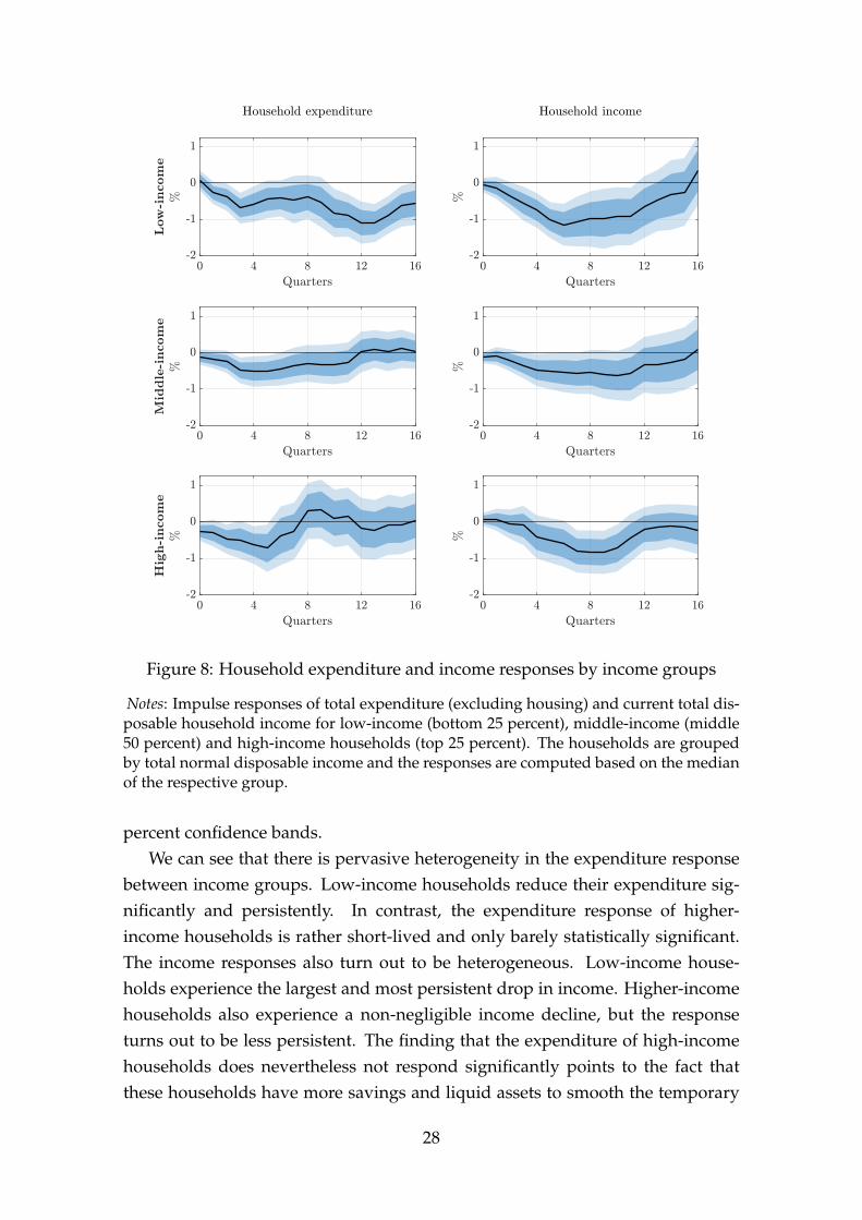
Figure 8: Household expenditure and income responses by income groups

Notes: Impulse responses of total expenditure (excluding housing) and current total dis-posable household income for low-income (bottom 25 percent), middle-income (middle50 percent) and high-income households (top 25 percent). The households are groupedby total normal disposable income and the responses are computed based on the medianof the respective group.

percent confidence bands.We can see that there is pervasive heterogeneity in the expenditure response

between income groups. Low-income households reduce their expenditure sig-nificantly and persistently. In contrast, the expenditure response of higher-income households is rather short-lived and only barely statistically significant.The income responses also turn out to be heterogeneous. Low-income house-holds experience the largest and most persistent drop in income. Higher-incomehouseholds also experience a non-negligible income decline, but the responseturns out to be less persistent. The finding that the expenditure of high-incomehouseholds does nevertheless not respond significantly points to the fact thatthese households have more savings and liquid assets to smooth the temporary

28

fall in their income. In contrast, the low-income households are hit twofold. First,they spend a larger share of their budget on energy and are thus, to the extent thatenergy expenditure is inelastic, adversely affected by the higher energy bill. Sec-ond, they experience a larger fall in income, as they tend to work in sectors thatare more strongly affected by the carbon policy shock (see Section 6.3). At thesame time, they are more likely to be financially constrained and less able to copewith the adverse effects on their income and budget.

Energy expenditure does indeed turn out to be pretty inelastic. Figure 9 showsthe responses of energy expenditure together with the responses of non-durablesexpenditure excluding energy and durables expenditure. We can see that the en-ergy bill increases substantially for all income groups, even though the responsesare not very precisely estimated.15 Thus, the fall in overall expenditure is notdriven by a drop in energy expenditure. In fact, the response of non-durable ex-penditure becomes even more pronounced after excluding energy expenditure,especially for lower-income households. Another way to see this is that the en-ergy share increases substantially for low-income households while it does notchange significantly for higher-income households (see Figures B.12-B.13 in theAppendix). The durables expenditure responses show a similar pattern to non-durables, with low-income households displaying the largest response. The mag-nitudes even turn out to be larger, in line with the fact that durables expendituretends to be more volatile. However, the responses also turn out to be less pre-cisely estimated. Thus, the fall in total expenditure appears to be largely drivenby the non-durable expenditure component.

At this stage, it is worth discussing a potential concern about grouping house-holds concerning selection. The assignments into the income groups are notrandom and some other characteristics may, potentially, be responsible for theheterogeneous responses I document. To mitigate these concerns, I group thehouseholds by a selection of other grouping variables, including age, educationand housing tenure. The results are shown in Figures B.19-B.21 in the Appendix.While there is not much heterogeneity by age, less educated households tendto respond more than better educated ones and social renters tend to respondmore than homeowners. However, none of the alternative grouping variablescan account for the patterns uncovered for income, suggesting that we are notspuriously picking up differences in other household characteristics.

15Note that energy expenditure is measured here as nominal expenditure, deflated by headlineHICP. The response of real energy expenditure, i.e. nominal expenditure deflated by the energycomponent of the HICP, tends to fall, in particular for middle- and high-income households (seeAppendix B.3.3 ).

29

Figure 9: Energy, non-durables and durables expenditure responses by income groups

Notes: Impulse responses of energy, non-durables excluding energy and durables expenditure for low-income (bottom 25 percent), middle-income (middle 50 percent) and high-income households (top 25 percent). The households are grouped by total normal disposable income andthe responses are computed based on the median of the respective group.

30

6.3. Direct versus indirect effects

We have seen that there is substantial heterogeneity in the households’ expendi-ture response to carbon policy shocks: while richer households change their ex-penditure only marginally, low-income households lower their expenditure sig-nificantly and persistently. Importantly, the magnitude of the response is muchlarger than what can be accounted for by the direct effect through higher energyprices. Assuming that energy demand is completely inelastic, the direct effectis bounded by the energy share of the respective group. However, the peak re-sponse of low-income households is around one – close to ten times the energyshare of that group. This suggests that indirect, general equilibrium effects viaincome and employment account for a large part of the overall effect on house-hold expenditure; a finding that is also supported by the significant effects onunemployment documented in Section 5.2.

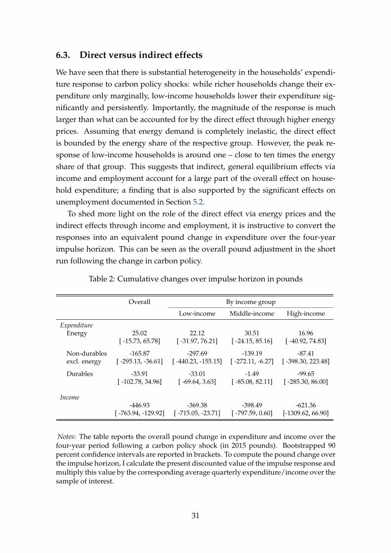
To shed more light on the role of the direct effect via energy prices and theindirect effects through income and employment, it is instructive to convert theresponses into an equivalent pound change in expenditure over the four-yearimpulse horizon. This can be seen as the overall pound adjustment in the shortrun following the change in carbon policy.

Table 2: Cumulative changes over impulse horizon in pounds

Overall By income group

Low-income Middle-income High-income

ExpenditureEnergy 25.02 22.12 30.51 16.96

[ -15.73, 65.78] [ -31.97, 76.21] [ -24.15, 85.16] [ -40.92, 74.83]

Non-durables -165.87 -297.69 -139.19 -87.41excl. energy [ -295.13, -36.61] [ -440.23, -155.15] [ -272.11, -6.27] [ -398.30, 223.48]

Durables -33.91 -33.01 -1.49 -99.65[ -102.78, 34.96] [ -69.64, 3.63] [ -85.08, 82.11] [ -285.30, 86.00]

Income-446.93 -369.38 -398.49 -621.36

[ -763.94, -129.92] [ -715.05, -23.71] [ -797.59, 0.60] [-1309.62, 66.90]

Notes: The table reports the overall pound change in expenditure and income over thefour-year period following a carbon policy shock (in 2015 pounds). Bootstrapped 90percent confidence intervals are reported in brackets. To compute the pound change overthe impulse horizon, I calculate the present discounted value of the impulse response andmultiply this value by the corresponding average quarterly expenditure/income over thesample of interest.

31

Table 2 shows the pound change in expenditure and income, overall and byincome group. We can see that energy expenditure increases significantly for allincome groups, but low-income households experience the largest increase rela-tive to their normal income. For these households, the energy bill increases byslightly more than 20 pounds while their income falls by close to 370 pounds.Importantly, their non-energy expenditure falls by around 330 pounds, which issubstantially larger than what can be accounted for by the increase in energy ex-penditure. This points to an important role of indirect effects via income and em-ployment. Interestingly, the pound increase in low-income households’ income isof a similar order of magnitude as the pound change in their expenditure. Whilemy empirical approach cannot shed light on the causal link between consumptionand income, this evidence is consistent with the notion that a considerable shareof low-income households have a high MPC and thus exhibit hand-to-mouth be-havior.

Higher-income households also experience a fall in their income (around 400pounds for middle-income and 620 pounds for high-income), however, the re-sponse is only barely statistically significant. Importantly, their expenditure fallsby much less and the response also turns out to be insignificant. This supportsthe notion that these households are less financially constrained and are thus ableto cushion the adverse effects on their income.

Overall, these results suggest that the direct effect through energy prices ac-counts for less than 20 percent of the overall effect on expenditure (25/174.8)while indirect effects via income account for over 80 percent (149.7/174.8).

The expenditure heterogeneity uncovered in this section is striking, especiallyagainst the backdrop that low-income households have much lower levels of ex-penditure to start with (see in Table 1). Put differently, low-income households ac-count for about 40 percent of the aggregate effect of carbon pricing on consump-tion, despite the fact that they make up for a much smaller share of consumptionin normal times (around 15 percent). Accounting for the indirect, general equi-librium effects turns out to be crucial to correctly assess the distributional impact.Focusing on the direct effect via the energy share alone can lead one to massivelyunderstate the actual distributional effects.

The stark distributional effects also likely play an important role for the sizeof the aggregate change in expenditure. My findings are consistent with a litera-ture that emphasizes the role of MPC heterogeneity in combination with unequalincome incidence for the transmission of aggregate demand shocks (Bilbiie, 2008,2020; Auclert, 2019; Patterson, 2021; Alves et al., 2020). These studies show in thecontext of aggregate-demand policies that the aggregate impact can be substan-

32

tially amplified when the policy disproportionately affects the incomes of indi-viduals whose consumption is more sensitive. My results suggest that a similarmechanism is at play in the transmission of carbon pricing, following the initialfall in non-energy expenditure. Thus, even though low-income households onlymake up for a relatively small portion of the population, they play an importantrole for the transmission to the macroeconomy and help explain the relativelylarge aggregate effects. In fact, in Section 7 I show that a model featuring theidentified transmission channels can account for the empirical evidence.

Alternative channels. Thus far, I focused my analysis on the direct effect via en-ergy prices and the indirect effect, general-equilibrium effect via income. Whilethere may also other channels at play, I briefly discuss here why these alternativechannels do not seem to play an important role in the transmission of carbon pol-icy. First, carbon pricing may also have an effect on the prices of other goods viasubstitution effects, which may in turn affect households’ budgets. However, asI have shown in Section 5.2, the response of core consumer prices is much moremuted and only barely significant; therefore this channel does likely not play amajor role. Second, there may be a number of channels that work through theresponse of durable expenditure, for instance because of uncertainty or precau-tionary motives, or via a reduction in durables that are complementary in usewith energy (see also Edelstein and Kilian, 2009). However, the overall responseof durable expenditure is quantitatively too small to play a dominant role in thetransmission of carbon policy. Furthermore, in Section 5.4 I did not find any sig-nificant change in aggregate uncertainty after the shock.

6.4. What drives the income response?

In the previous section, I document that unequal income incidence in combina-tion with heterogeneous MPCs appears to play a key role in the transmission ofcarbon policy shocks. This section aims to shed more light on what is driving theincome incidence by household group. There are at least two potential sourcesof heterogeneity. First, households may differ in their labor income, for instancebecause they tend to work in different sectors. Second, some households mayalso have financial income, such as rental income or dividends, whereas othershave to rely uniquely on their labor income.

To investigate into potential heterogeneities in labor income, I study how theresponses vary by the sector of employment using data from the UK Labour Force

33

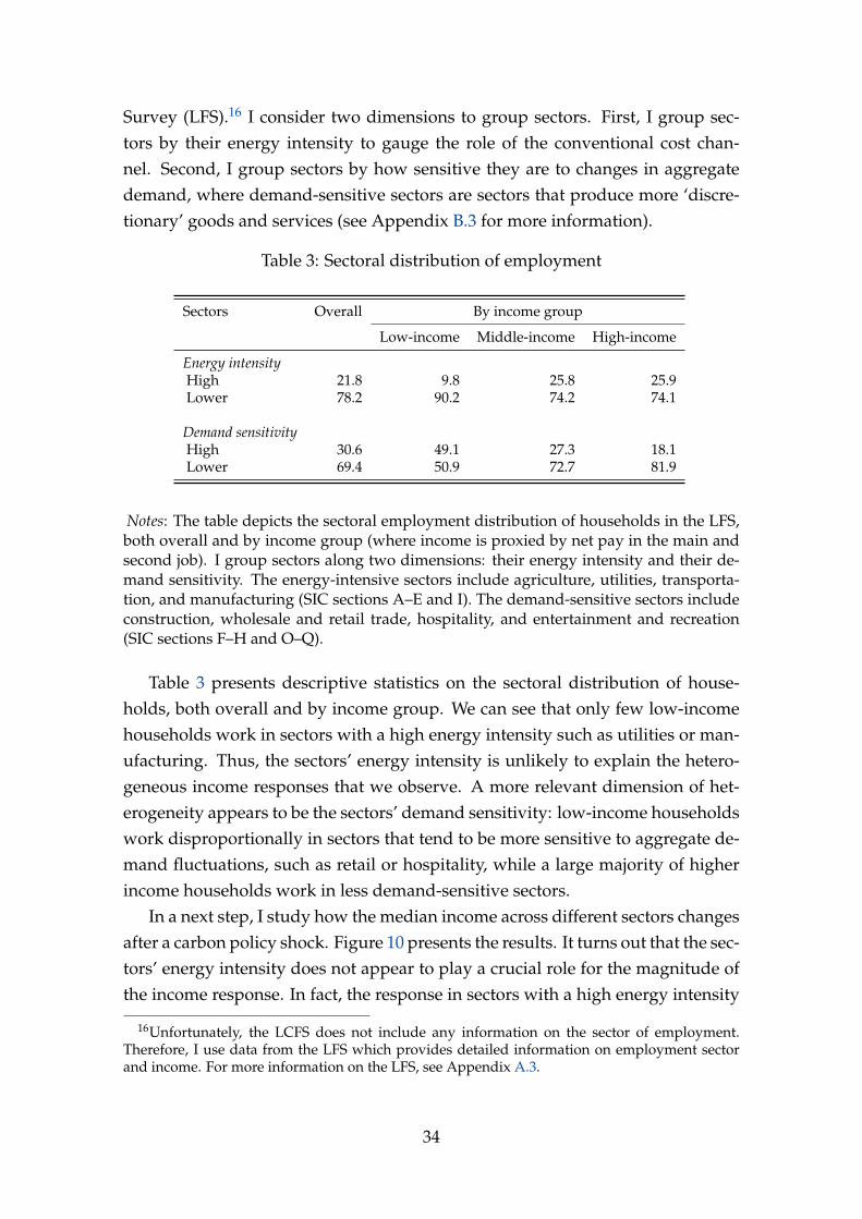
Survey (LFS).16 I consider two dimensions to group sectors. First, I group sec-tors by their energy intensity to gauge the role of the conventional cost chan-nel. Second, I group sectors by how sensitive they are to changes in aggregatedemand, where demand-sensitive sectors are sectors that produce more ‘discre-tionary’ goods and services (see Appendix B.3 for more information).

Table 3: Sectoral distribution of employment

Sectors Overall By income group

Low-income Middle-income High-income

Energy intensityHigh 21.8 9.8 25.8 25.9Lower 78.2 90.2 74.2 74.1

Demand sensitivityHigh 30.6 49.1 27.3 18.1Lower 69.4 50.9 72.7 81.9

Notes: The table depicts the sectoral employment distribution of households in the LFS,both overall and by income group (where income is proxied by net pay in the main andsecond job). I group sectors along two dimensions: their energy intensity and their de-mand sensitivity. The energy-intensive sectors include agriculture, utilities, transporta-tion, and manufacturing (SIC sections A–E and I). The demand-sensitive sectors includeconstruction, wholesale and retail trade, hospitality, and entertainment and recreation(SIC sections F–H and O–Q).

Table 3 presents descriptive statistics on the sectoral distribution of house-holds, both overall and by income group. We can see that only few low-incomehouseholds work in sectors with a high energy intensity such as utilities or man-ufacturing. Thus, the sectors’ energy intensity is unlikely to explain the hetero-geneous income responses that we observe. A more relevant dimension of het-erogeneity appears to be the sectors’ demand sensitivity: low-income householdswork disproportionally in sectors that tend to be more sensitive to aggregate de-mand fluctuations, such as retail or hospitality, while a large majority of higherincome households work in less demand-sensitive sectors.

In a next step, I study how the median income across different sectors changesafter a carbon policy shock. Figure 10 presents the results. It turns out that the sec-tors’ energy intensity does not appear to play a crucial role for the magnitude ofthe income response. In fact, the response in sectors with a high energy intensity

16Unfortunately, the LCFS does not include any information on the sector of employment.Therefore, I use data from the LFS which provides detailed information on employment sectorand income. For more information on the LFS, see Appendix A.3.

34

Figure 10: Income response by sector of employment

Notes: Impulse responses of income (pay from main and second job net of deduc-tions and benefits) in different sectors, grouped by their energy-intensity and demand-sensitivity. The response is computed based on the median income in the respectivegroup of sectors. The sector groups are described in detail in Table 3.

is relatively comparable to the response in sectors with a lower energy intensity.17

In contrast, there is significant heterogeneity by the sectors’ demand-sensitivity:households working in demand-sensitive sectors experience the largest and mostsignificant fall in their income after a carbon policy shock while households inless-demand sensitive sectors face a much more muted income response.

These results support the interpretation that carbon policy shocks mainlytransmit to the economy through the demand side, and not by affecting produc-tion costs. While this may seem surprising, it is in line with previous evidence byKilian and Park (2009) on the transmission of energy price shocks. Importantly,the results also help explain why low-income households display a stronger fallin their income, as they disproportionally work in demand-sensitive sectors. Inresponse to a carbon policy shock, these sectors face a stronger decrease in de-mand than other sectors, also because low-income households cut expendituremore in these sectors, and thus react by laying off employees and cutting com-pensation.

17Note that I exclude utilities from the energy-intensive group, as there is reason to believethat the utility sector behaves differently from other energy-intensive sectors. In fact, as shownin Figure B.23 in the Appendix, the utility sector does not display a significant fall in incomes, inline with the findings from Section 5.4.

35

Another important difference between low- and high-income households liesin the income composition. While low- and middle-income households mainlyrely on labor income, high-income households also have significant financial in-come. Figure B.24 in the Appendix shows the response of financial income bythe three income groups we consider. We can see that financial income barelyresponds for low- and middle-income households, consistent with the fact thatthese households only have very little financial income. By contrast, the financialincome response of high-income households is both statistically and economi-cally significant. Consistent with the stock market response reported in Section 5,their financial income falls for about one year but then reverses and turns signifi-cantly positive.

6.5. Policy implications

We have documented substantial heterogeneity in the response of householdsto carbon policy shocks. The findings illustrate that the economic costs of car-bon pricing are not borne equally across society. It is the lower-income house-holds that are the most affected, having to reduce their expenditures the most,and that are driving the aggregate response. My results highlight the impor-tance of energy prices in the transmission of carbon policy shocks through directand indirect channels that disproportionally affect lower-income households –the very households that also tend to be financially constrained and have a highermarginal propensity to consume. In this sense, I show that carbon pricing trans-mits through a powerful demand channel that can outweigh the traditional costchannel by an order of magnitude. This result speaks directly to a growing litera-ture on the role of Keynesian supply shocks (see e.g. Guerrieri et al., forthcoming;Cesa-Bianchi and Ferrero, 2021).

My findings suggest that fiscal policies targeted to the most affected house-holds can reduce the economic costs of climate change mitigation policies andameliorate the trade-off between reducing emissions and maintaining economicactivity. To the extent that energy demand is inelastic, which turns out to be par-ticularly the case for low-income households, this should not compromise thereductions in emissions.

Such a policy could be implemented for instance by recycling some of the rev-enues generated from auctioning allowances. While in the first two phases ofthe ETS, the majority of allowances was freely allocated, auctioning became thedefault in the third phase, generating substantial auction revenues. For the pe-riod from 2012-2020, the revenues generated by the member states of the EU ETSexceeded 57 billion euros (European Comission, 2020b). The ETS directive from

36

2008 states that at least half of the auction revenues should be used for climateand energy related purposes and indeed, over the period 2013-2019 close to 80percent of auction revenues were used for such purposes. While this should helpto further propel emission reductions, my results indicate that by redistributingpart of the auction revenues to the most affected groups in society, it is possi-ble to mitigate the distributional effects and reduce the economic costs of climatepolicy.18

Another important argument for cushioning the distributional impact is thata successful transition to a low-carbon economy requires public support. If cer-tain groups feel left behind, this could undermine the success of climate policyas the yellow vest movement in France, which started as a protest against higherfuel taxes, has shown for instance (see also Knittel, 2014). Indeed, in AppendixB.3 I provide some empirical evidence that carbon policy shocks lead to a de-crease in the public support of climate policy. While the support among low-income households falls significantly and persistently, the response of higher-income households is more short-lived and even turns positive at longer hori-zons. These results suggest that compensating low-income households that aremore exposed to carbon pricing may indeed help to increase the public supportof climate change mitigation policies – consistent with recent evidence by Ander-son, Marinescu, and Shor (2019).

7. A heterogeneous-agent climate-economy model

To study the role of redistributing carbon revenues more formally, I build aclimate-economy model. The aim is to obtain a framework that can account forthe empirical findings – both in the aggregate and along the cross section – andcan be used as a laboratory for policy experiments. The model belongs to thedynamic stochastic general equilibrium (DSGE) class. It augments the climate-economy structure by Golosov et al. (2014) with nominal rigidities, householdheterogeneity and risk to allow for the demand channels identified in the data.The model consists of four building blocks: households, firms, a government anda climate block. I outline the model here, a more detailed description can befound in Appendix D.

18The current ETS does not feature such a direct redistribution scheme, however, there are cer-tain other, indirect solidarity measures in place, e.g. via the Cohesion Fund or the Just TransitionFund. Only in the recent ‘Fit for 55’ plan, the European Commission takes a step in this directionby proposing a new Social Climate Fund. However, the proposed fund will be limited to the newemissions trading system for building and transport fuels, and only includes an amount equiva-lent to 25 percent of the expected revenues (European Comission, 2021).

37

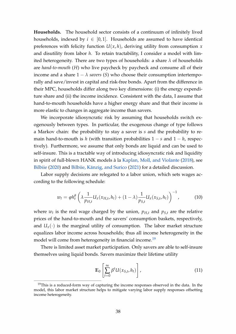
Households. The household sector consists of a continuum of infinitely livedhouseholds, indexed by i ∈ [0, 1]. Households are assumed to have identicalpreferences with felicity function U(x, h), deriving utility from consumption xand disutility from labor h. To retain tractability, I consider a model with lim-ited heterogeneity. There are two types of households: a share λ of householdsare hand-to-mouth (H) who live paycheck by paycheck and consume all of theirincome and a share 1− λ savers (S) who choose their consumption intertempo-rally and save/invest in capital and risk-free bonds. Apart from the difference intheir MPC, households differ along two key dimensions: (i) the energy expendi-ture share and (ii) the income incidence. Consistent with the data, I assume thathand-to-mouth households have a higher energy share and that their income ismore elastic to changes in aggregate income than savers.

We incorporate idiosyncratic risk by assuming that households switch ex-ogenously between types. In particular, the exogenous change of type followsa Markov chain: the probability to stay a saver is s and the probability to re-main hand-to-mouth is h (with transition probabilities 1 − s and 1 − h, respec-tively). Furthermore, we assume that only bonds are liquid and can be used toself-insure. This is a tractable way of introducing idiosyncratic risk and liquidityin spirit of full-blown HANK models à la Kaplan, Moll, and Violante (2018), seeBilbiie (2020) and Bilbiie, Känzig, and Surico (2021) for a detailed discussion.

Labor supply decisions are relegated to a labor union, which sets wages ac-cording to the following schedule:

wt = ϕhθt

(λ

1pH,t

Ux(xH,t, ht) + (1− λ)1

pS,tUx(xS,t, ht)

)−1

, (10)

where wt is the real wage charged by the union, pH,t and pS,t are the relativeprices of the hand-to-mouth and the savers’ consumption baskets, respectively,and Ux(·) is the marginal utility of consumption. The labor market structureequalizes labor income across households; thus all income heterogeneity in themodel will come from heterogeneity in financial income.19

There is limited asset market participation. Only savers are able to self-insurethemselves using liquid bonds. Savers maximize their lifetime utility

E0

[∞

∑t=0

βtU(xS,t, ht)

], (11)

19This is a reduced-form way of capturing the income responses observed in the data. In themodel, this labor market structure helps to mitigate varying labor supply responses offsettingincome heterogeneity.

38

choosing how much to consume xS,t, save bS,t+1 and invest iS,t. Their con-sumption bundle xS,t is a composite of a non-energy good cS,t and energy eS,t:

xS,t =

(a

1εxS,cc

εx−1εx

S,t + a1

εxS,ee

εx−1εx

S,t

) εxεx−1

, where aS,c and aS,e are distribution parameters

satisfying aS,c + aS,e = 1, and εx is the elasticity of substitution between non-energy and energy goods. This gives rise to standard non-energy and energy

demand functions: cS,t = aS,c

(1

pS,t

)−εxxS,t and eS,t = aS,e

(pe,tpS,t

)−εxxS,t.

The savers budget constraint equates their consumption, savings and invest-ment to their income, accounting for the flows of liquid assets between types (see

Appendix D for details). Their income is given by yS,t = wtht +Rb

t−1Πt

bS,t + (1−τk)rtkS,t +

(1−τd)dt1−λ + ωS,t, where pS,t is the price of the savers’ final consumption

bundle,Rb

t−1Πt

is the risk-free rate deflated by inflation, rt is the rental rate of capital,dt are dividends, and ωS,t are transfers from the government. Capital accumula-tion follows kS,t+1 = iS,t + (1− δ)kS,t.

Maximizing (11) subject to the budget constraint and the capital accumulationequation, we obtain the Euler equations for investment and bond holdings:

λS,t = β Et

[(1 + (1− τk)rt+1 − δ)λS,t+1

](12)

λS,t = β Et

[Rb

tΠt+1

(sλS,t+1 + (1− s)λH,t+1)

], (13)

where λi,t =Ux(xi,t,ht)

pi,tfor i ∈ S, H. Note that only the Euler equation for bonds

includes the marginal utility in the H-state, reflecting the fact that only bonds areliquid and can be used to self-insure against idiosyncratic risk.

Hand-to-mouth households have no assets and thus consume all of their in-come in every period:

pH,txH,t = yH,t. (14)

The income of the hand-to-mouth is given by yH,t = wthdt + ωH,t, where ωH,t

are government transfers. The non-energy and energy demand functions and theassociated price index are analogous to the expressions for the savers.

Firms. The firm block of the model consists of two sectors: energy and non-energy producers. Energy firms produce energy using labor as an input. Non-energy firms produce the non-energy consumption good using capital, energy,and labor as inputs. Consistent with the data, we assume that energy firms canadjust their prices flexibly while non-energy firms face nominal price rigidities

39

(Dhyne et al., 2006).The energy firm produces energy according to the following technology

et = ae,the,t, (15)

as in Golosov et al. (2014). I assume that there is only a single source of energy(e.g. coal) that is available in approximately infinite supply. Without loss of gen-erality, energy is measured in terms of carbon content (carbon amount emitted).Energy firms are subject to a carbon sales tax τt.20 The optimal energy supply ischaracterized by wt = (1− τt)pe,t

ethe,t

.The non-energy sector consists of standard New Keynesian firms that pro-

duce different varieties of non-energy goods and set prices subject to nominalrigidities. The final non-energy good is assembled by a CES aggregator.

The non-energy variety j is produced according to the following technology,using capital kt(j), energy ey,t(j), and labor hy,t(j) as inputs

yt(j) = e−γst atkt(j)αey,t(j)νhy,t(j)1−α−ν, (16)

where at is a technology shifter. The function e−γst , where st is the atmosphericcarbon concentration, captures climate damages. This generates a feedback loopbetween climate and the economy. Higher economic activity increases carbonemissions via higher energy use, which in turn increases the carbon concentra-tion. A higher carbon concentration will have economic damages in turn (e.g.via weather events etc.), which reduce output. The functional form is taken fromGolosov et al. (2014), where γ governs the size of climate damages.

The cost-minimization problem gives rise to the standard factor demands forcapital rt = αmct

ytkt

, energy pe,t = νmctytey,t

, and labor wt = (1 − α − ν)mctyt

hy,t,

where mct are real marginal costs. Note that factor demands are common acrossfirms.

The price setting problem gives rise to a standard Phillips curve, which inlog-linear form reads πt = κmct + βEtπt+1, where hatted variables denote log-deviations from steady state. Finally, profits are given by dt =

∫ 10 [

Pt(j)Pt

yt(j) −mctyt(j)]dj.

20For simplicity, we consider here a carbon tax, howvever, we could equivalently consider reg-ulating the quantity (see e.g. the discussion in Heutel, 2012).

40

Climate block. As in Golosov et al. (2014), the current level of atmospheric car-bon concentration as a function of current and past emissions:

st =∞

∑s=0

(1− ds)et−s, with 1− ds = (1− ϕL)ϕ0(1− ϕ)s. (17)

Here, 1− ϕ0 is the share of remaining emissions exiting the atmosphere immedi-ately while ϕ0 is the remaining share of emissions that decay over time at a geo-metric rate 1− ϕ. We can write this in recursive form as st = (1− ϕ)st−1 + ϕ0et.

Fiscal and monetary policy. The government runs a balanced budget in everyperiod, i.e. all transfers are financed by tax revenues. We consider the followingtransfer policy

λωH,t = τddt + τkrKt kt + µτt pe,tet and (1− λ)ωS,t = (1− µ)τt pe,tet. (18)

The distribution of carbon tax revenues are governed by parameter µ.21 Carbontaxes τt are set according to the following rule: τt = (1− ρτ)τ + ρττt−1 + ετ,t.

Finally, we assume that there is a monetary authority that conducts monetarypolicy according to the following Taylor rule (in log-linear form): rb

t = ρr rbt−1 +

(1− ρr)(φππT,t + φyyt) + εmp,t, where πT,t is headline inflation.

Functional forms and calibration. The felicity function is of the standard CRRA

form U(xi,t, ht) =x1−σ

i,t −11−σ − ψ

h1+θt

1+θ . The model is calibrated using both macro andmicro moments estimated from the data. The time period is a quarter. I setβ = 0.99 and σ = θ = 0.5. The share of hand-to-mouth is λ = 0.25. Idiosyn-cratic risk is calibrated to 1− s = 0.04. These values are all commonly used inthe literature. The parameters aH,e and aS,e are calibrated to match the energyexpenditure shares in the LCFS. Energy and non-energy goods are modeled asweak complements, εx = 0.75. Turning to the production side, I set δ = 0.025,and α and ν are calibrated to match the capital and energy share in the data. Thesteady-state markup is assumed to be 20 percent and the average price spell is5-6 quarters. The climate block is calibrated as in Golosov et al. (2014). Turning tofiscal and monetary policy, the steady-state carbon tax is calibrated to 4 percent,the implied average tax rate in the EU ETS. The Taylor rule coefficient on infla-tion and output are 1.75 and 0.25, respectively, and the interest rate smoothingparameter is 0.6. I discuss the calibration in detail in Appendix D.8.

21As the baseline, we assume that all carbon revenues accrue to the savers µ = 0. Later, we willstudy alternative transfer policies. Furthermore, we set τd = τk = 0 as the baseline. These taxeswill later be used to equalize incomes over the cycle by setting τd = τk = µ = λ.

41

7.1. Model evaluation

The impulse responses to a carbon policy shock, normalized to increase the en-ergy price by 1 percent on impact, are shown in Figure 11. We can see that themodel is successful in generating peak responses of consumption and income, inthe aggregate and by household group, that are in the same order of magnitudeas the estimated responses in Section 6. As in the data, consumption and incomeare more responsive to carbon policy shocks for the low-income, hand-to-mouthhouseholds, with a peak response of around -1 percent. In contrast, the incomeand in particular the consumption response of the high-income savers is muchless pronounced.

Figure 11: Consumption and income responses

Notes: Impulse responses of consumption and income, in the aggregate as well as forhand-to-mouth and savers, to a carbon policy shock normalized to increase the energyprice by 1 percent on impact. The blue line is the baseline response when carbon revenuessolely accrue to the savers; the red dashed line is the response when carbon revenues areredistributed equally among hand-to-mouth and savers.

42

Table 4: Direct versus indirect effects in model and data

Overall By household group

Low-income/ Higher-income/Hand-to-mouth Savers

ModelDirect 11.1 2.0 25.5Indirect 88.9 98.0 74.5

DataDirect 14.3 7.2 20.3Indirect 85.7 92.8 79.7

Notes: The table contrasts the role of the direct effect via energy prices and the indirecteffects via income in the model and in the data. As in Section 6.3, the strength of the directis measured by the share in the overall decrease in consumption that can be attributed tothe increase in energy expenditure. In the model, the overall adjustment in consumptionand energy expenditure are computed as the present discounted value of the impulseresponse multiplied by the corresponding steady state value.

Most importantly, we can also look at the importance of direct and indirecteffects through the lens of the model. Table 4 computes the shares of the directeffect via the increase in energy expenditure and the indirect effects via income,both in the aggregate and by household group. These contributions are calculatedin the exact same way as in data (see Section 6.3 for more information).

We can see that the bulk of the effect on aggregate consumption in the model isdriven by the indirect effects via income. The role of indirect effects is particularlystark for the hand-to-mouth while for savers, the direct effect also explains a non-negligible portion. Contrasting the contributions of the different channels withthe ones estimated from the UK survey data in Section 6.3, we can see that themodel is able to match the estimated contributions remarkably well.

Overall, these results illustrate that a climate-economy model featuring thekey dimensions of heterogeneity identified from the empirical evidence can gen-erate effects that are in the same ballpark as in the data, both in terms of abso-lute magnitude and relative importance of direct and indirect effects. Householdheterogeneity turns out to be key for this result. Without the heterogeneity chan-nels, it practically infeasible to match the sizeable responses observed in the datawithout calibrating the energy expenditure share to implausibly high levels, seeAppendix B.4.

43

7.2. Redistributing carbon revenues

Having evaluated the empirical performance of the model, we are now in a po-sition to study how different carbon revenue redistribution schemes affect thetransmission of carbon pricing. Figure 11 compares the baseline case when allcarbon revenues accrue to the savers (blue line) to the case where the revenuesare distributed equally across households µ = λ (red dashed line).

We can see that redistributing carbon revenues leads to a reduction in con-sumption inequality as the consumption of hand-to-mouth falls by less while theconsumption of savers falls by somewhat more than in the baseline case. Thishas also consequences for the effect on aggregate consumption: the total effectis around 15 percent smaller than in the baseline case of no redistribution. Incontrast, redistributing revenues has a fairly minor impact on the response ofemissions, see Appendix B.4. The intuition is that the redistribution scheme sup-ports the income of the hand-to-mouth which in turn supports their consumptionto a significant extent as they have a high MPC. Savers, on the other hand, face asomewhat more pronounced fall in their income but the effect on their consump-tion is more muted as they are able to better smooth the effects of the shock.

The above findings speak directly to the recent debate on carbon pricing andinequality in Europe. The climate-economy model with heterogeneous agentsconfirms the intuition that redistributing carbon revenues could mitigate the ef-fect on aggregate consumption and alleviate the distributional impact withoutcompromising emission reductions. In future work, it would be interesting tobetter understand the implications of the demand channels of carbon policy iden-tified in this paper for optimal climate policy. To the extent that the distributionaleffects are larger when accounting for the indirect effects via income, we may alsoexpect the welfare costs of carbon pricing to be larger.

8. Sensitivity analysis

In this section, I perform a number of robustness checks on the identificationstrategy and the empirical specification used to isolate the carbon policy shock.The main results of these checks are summarized below. More information aswell as the corresponding figures and tables can be found in Appendix B.5.

Selection of relevant events. A crucial choice in the high-frequency event studyapproach concerns the selection of relevant events. For the exclusion restriction tobe satisfied, the events should only release information about the supply of emis-

44

sion allowances and not about other factors such as macroeconomic or geopo-litical news. To this end, I have not included broader events such as the Parisagreement or other COP meetings but limited the analysis to specific events in theEuropean carbon market. The most obvious candidates are events about the freeallocation and auctioning of emission allowances. I have also included events onthe overall cap in the carbon market as well as events about international credits.

Because the events concerning the cap tend to be broader in nature, I excludethese events as a robustness check. As shown in Figure B.31, the results turn outto be robust. I have also tried to exclude the events about international credits,which affect the supply of allowances only indirectly, by changing the number ofcredits from international projects that can be exchanged for allowances. FromFigure B.32, we can see that the results turn out to be very similar. By goingthrough all events in detail, I could also identify some events that are poten-tially confounded, either because some other event happened on the same day(more on this below) or because they could potentially also contain some infor-mation about demand in the carbon market. Reassuringly, however, excludingthese events does not change the results materially (see Figure B.34). Finally, Ihave verified that the identification strategy does not hinge upon extreme events.Excluding the largest surprises (price change in excess of 30 percent) does notchange the results materially, even though the responses are less precisely esti-mated (see Figure B.35).

Confounding news. Another important choice in high-frequency identificationconcerns the size of the event window. As discussed in Section 3, there is a trade-off between capturing the entire response to the policy news and backgroundnoise, i.e. the threat of other news confounding the response. Common windowchoices range from 30-minutes to multiple days. Unfortunately, the exact releasetimes are unavailable for the majority of the policy events considered, making itinfeasible to use an intraday window. Therefore, I use a daily window to computethe policy surprises.

To mitigate concerns about other news confounding the carbon policy sur-prise series, I employ an alternative identification strategy exploiting the het-eroskedasticity in the data (Rigobon, 2003; Nakamura and Steinsson, 2018). Theidea is to clean out the background noise in the surprise series by compar-ing movements in carbon prices during policy event windows to other equallylong and otherwise similar event windows that do not contain a regulatory up-date event. In particular, I use the changes in carbon futures prices on thesame weekday and week in the months prior a given regulatory event. An

45

overview of announcement and control dates can be found in Table B.6 in theAppendix. More details on the underlying assumptions and how to implementthe heteroskedasticity-based approach are provided in Appendix C.

Figure B.36 shows the carbon policy surprise series together with the controlseries. We can see that the policy surprise series is over six times more volatilethan the control series. It is exactly this shift in variance that can be exploited foridentification, assuming that the shift is driven by the carbon policy shock. Fig-ure B.37 shows the impulse responses estimated from this alternative approach.The results turn out to be consistent with the baseline results from the external in-strument approach, even though the responses are a bit less precisely estimated.These results suggest that the bias induced by background noise is likely negligi-ble in the present application.

Sample and specification choices. An important robustness check concerns theestimation sample. Recall, the baseline sample goes back to 1999, which is longerthan the instrument sample which only starts in 2005. The main motivation forusing the longer sample is to increase the precision of the estimates. As a robust-ness check, I restrict the overall sample to the 2005-2018 period. The responsesare shown in Figure B.39. Overall, the results are very similar to the ones us-ing the longer sample. However, some responses turn out to be a bit less stable,which could point to difficulties in estimating the model dynamics on the rela-tively short sample.

Another interesting check concerns the sample for the carbon policy surprises.Recall that the EU ETS was established in phases and the first phase was a pilotphase. As a robustness test, I exclude the regulatory news from this first phase.From Figure B.40, we can see that the point estimates turn out to be quite similar.However, as probably had to be expected the responses are much less preciselyestimated. This illustrates nicely how the identification strategy leverages thefact that establishing the carbon market was a learning-by-doing process wherethe rules have been continuously updated.

I also perform a number of sensitivity checks on the specification of the model.The baseline VAR includes 8 variables, which is relatively large, especially giventhe short sample. As a robustness test, I use a 6-variable model, excluding stockprices and the real exchange rate. As can be seen from Figure B.41, the resultsfrom this smaller model turn out to be very similar to the larger baseline model.The results also turn out to be robust to the lag order (Figures B.43-B.44 show theresponses using 3 or 9 lags) and the choice of deterministics (Figure B.42 includesa linear trend). Finally, I also present results from a Bayesian VAR model with 12

46

lags and using shrinkage priors. The results turn out to be again very similar tothe baseline VAR (see Figure B.45).

9. Conclusion

Fighting climate change is one of the greatest challenges of our time. Whileit has proved to be very difficult to make progress at the global level, severalnational carbon pricing policies have been put in place. However, still little isknown about the effects of these policies on emissions and the economy. Thispaper provides new evidence on the effects of carbon pricing from the largestcarbon market in the world, the EU ETS. I show that tightening the carbon pric-ing regime leads to a persistent fall in emissions and a significant increase inenergy prices. The fall in emissions comes at the cost of temporarily lower eco-nomic activity. The results point to a strong transmission mechanism workingthrough energy prices leading to lower consumption and investment. Impor-tantly, these economic costs are not borne equally across society. Lower-incomehouseholds lower their consumption significantly and are driving the aggregateresponse while richer households are less affected. Not only are these house-holds more exposed to carbon pricing because of their higher energy expenditureshare, they also experience a larger fall in their income. These indirect effects viaincome and employment play a crucial role in the transmission, accounting forover 80 percent of the aggregate effect on consumption. My results suggest thatre-distributing some of the auction revenues to the most affected groups in soci-ety may be an effective way to reduce the economic costs of carbon pricing andstrengthen the public support of the policy.

References

Alves, Felipe, Greg Kaplan, Benjamin Moll, and Giovanni L. Violante. 2020. “A further

look at the propagation of monetary policy shocks in HANK.” Journal of Money, Creditand Banking, 52(S2): 521–559.

Anderson, Soren T., Ioana Marinescu, and Boris Shor. 2019. “Can Pigou at the Polls

Stop Us Melting the Poles?”

Andersson, Julius J. 2019. “Carbon Taxes and CO2 Emissions: Sweden as a Case Study.”

American Economic Journal: Economic Policy, 11(4): 1–30.

Annicchiarico, Barbara and Fabio Di Dio. 2015. “Environmental policy and macroeco-

nomic dynamics in a new Keynesian model.” Journal of Environmental Economics andManagement, 69: 1–21.

47

Auclert, Adrien. 2019. “Monetary policy and the redistribution channel.” American Eco-nomic Review, 109(6): 2333–67.

Barnichon, Regis and Christian Brownlees. 2019. “Impulse response estimation by

smooth local projections.” Review of Economics and Statistics, 101(3): 522–530.

Baumeister, Christiane and Lutz Kilian. 2017. “A general approach to recovering market

expectations from futures prices with an application to crude oil.”

Bernard, Jean-Thomas and Maral Kichian. 2021. “The Impact of a Revenue-Neutral Car-

bon Tax on GDP Dynamics: The Case of British Columbia.” The Energy Journal, 42(3).

Beznoska, Martin, Johanna Cludius, and Viktor Steiner. 2012. “The incidence of the Eu-

ropean Union Emissions Trading System and the role of revenue recycling: Empirical

evidence from combined industry-and household-level data.”

Bilbiie, Florin O. 2008. “Limited asset markets participation, monetary policy and (in-

verted) aggregate demand logic.” Journal of Economic Theory, 140(1): 162–196.

Bilbiie, Florin O. 2020. “Monetary Policy and Heterogeneity: An Analytical Frame-

work.”

Bilbiie, Florin O., Diego R. Känzig, and Paolo Surico. 2021. “Capital and income in-

equality: An aggregate-demand complementarity.”

Blanchard, Olivier J. and Roberto Perotti. 2002. “An empirical characterization of the

dynamic effects of changes in government spending and taxes on output.” The Quar-terly Journal of Economics, 117(4): 1329–1368.

Browning, Martin, Angus Deaton, and Margaret Irish. 1985. “A profitable approach to

labor supply and commodity demands over the life-cycle.” Econometrica, 503–543.

Bushnell, James B., Howard Chong, and Erin T. Mansur. 2013. “Profiting from regu-

lation: Evidence from the European carbon market.” American Economic Journal: Eco-nomic Policy, 5(4): 78–106.

Calel, Raphael and Antoine Dechezleprêtre. 2016. “Environmental policy and directed

technological change: evidence from the European carbon market.” Review of Eco-nomics and Statistics, 98(1): 173–191.

Cesa-Bianchi, Ambrogio and Andrea Ferrero. 2021. “The transmission of Keynesian

supply shocks.”

Cloyne, James. 2013. “Discretionary tax changes and the macroeconomy: new narrative

evidence from the United Kingdom.” American Economic Review, 103(4): 1507–28.

Cloyne, James and Paolo Surico. 2017. “Household debt and the dynamic effects of in-

come tax changes.” The Review of Economic Studies, 84(1): 45–81.

Cloyne, James, Clodomiro Ferreira, and Paolo Surico. 2020. “Monetary policy when

households have debt: new evidence on the transmission mechanism.” The Review ofEconomic Studies, 87(1): 102–129.

DEHSt, German Emissions Trading Authority. 2019. “German Auctioning of Emission

Allowances: Periodical Report: Annual Report 2018.”

Dhyne, Emmanuel, Luis J. Alvarez, Hervé Le Bihan, Giovanni Veronese, Daniel Dias,

48

Johannes Hoffmann, Nicole Jonker, Patrick Lunnemann, Fabio Rumler, and JoukoVilmunen. 2006. “Price changes in the euro area and the United States: Some facts

from individual consumer price data.” Journal of Economic Perspectives, 20(2): 171–192.

Edelstein, Paul and Lutz Kilian. 2009. “How sensitive are consumer expenditures to

retail energy prices?” Journal of Monetary Economics, 56(6): 766–779.

European Comission. 2020a. “EU Emissions Trading System (EU ETS).” https: // ec.

europa. eu/ clima/ policies/ ets_ en , [Online; accessed 02-Dec-2020].

European Comission. 2020b. “Report on the functioning of the European carbon mar-

ket.” https: // ec. europa. eu/ clima/ sites/ clima/ files/ news/ docs/ com_ 2020_

740_ en. pdf , [Online; accessed 02-Dec-2020].

European Comission. 2021. “Fit for 55: delivering the EU’s 2030 Climate Target on the

way to climate neutrality.” https: // eur-lex. europa. eu/ legal-content/ EN/ TXT/

?uri= CELEX: 52021DC0550 , [Online; accessed 30-Aug-2021].

Fan, Ying, Jun-Jun Jia, Xin Wang, and Jin-Hua Xu. 2017. “What policy adjustments in

the EU ETS truly affected the carbon prices?” Energy Policy, 103: 145–164.

Gertler, Mark and Peter Karadi. 2015. “Monetary policy surprises, credit costs, and eco-

nomic activity.” American Economic Journal: Macroeconomics, 7(1): 44–76.

Golosov, Mikhail, John Hassler, Per Krusell, and Aleh Tsyvinski. 2014. “Optimal taxes

on fossil fuel in general equilibrium.” Econometrica, 82(1): 41–88.

Goulder, Lawrence and Marc Hafstead. 2018. Confronting the Climate Challenge.Columbia University Press.

Guerrieri, Veronica, Guido Lorenzoni, Ludwig Straub, and Iván Werning. forthcom-

ing. “Macroeconomic implications of COVID-19: Can negative supply shocks cause

demand shortages?” American Economic Review.

Gürkaynak, Refet S., Brian Sack, and Eric T. Swanson. 2005. “Do actions speak louder

than words? The response of asset prices to monetary policy actions and statements.”

International Journal of Central Banking, 1: 55–93.

Hamilton, James D. 2008. “Oil and the macroeconomy.” The New Palgrave Dictionary ofEconomics, 2.

Hamilton, James D. 2009. “Daily changes in fed funds futures prices.” Journal of Money,credit and Banking, 41(4): 567–582.

Heutel, Garth. 2012. “How should environmental policy respond to business cycles?

Optimal policy under persistent productivity shocks.” Review of Economic Dynamics,

15(2): 244–264.

Jentsch, Carsten and Kurt G. Lunsford. 2019. “The dynamic effects of personal and cor-

porate income tax changes in the United States: Comment.” American Economic Review,

109(7): 2655–78.

Johnson, David S., Jonathan A. Parker, and Nicholas S. Souleles. 2006. “Household Ex-

penditure and the Income Tax Rebates of 2001.” American Economic Review, 96(5): 1589–

1610.

49

Jordà, Òscar, Moritz Schularick, and Alan M. Taylor. 2015. “Betting the house.” Journalof International Economics, 96: S2–S18.

Kaplan, Greg and Giovanni L. Violante. 2014. “A model of the consumption response

to fiscal stimulus payments.” Econometrica, 82(4): 1199–1239.

Kaplan, Greg, Benjamin Moll, and Giovanni L. Violante. 2018. “Monetary policy ac-

cording to HANK.” American Economic Review, 108(3): 697–743.

Kilian, Lutz and Cheolbeom Park. 2009. “The impact of oil price shocks on the US stock

market.” International Economic Review, 50(4): 1267–1287.

Knittel, Christopher R. 2014. “The Political Economy of Gasoline Taxes: Lessons from

the Oil Embargo.” Tax Policy and the Economy, 28(1): 97–131.

Konradt, Maximilian and Beatrice Weder di Mauro. 2021. “Carbon Taxation and Infla-

tion: Evidence from the European and Canadian Experience.”

Kuttner, Kenneth N. 2001. “Monetary policy surprises and interest rates: Evidence from

the Fed funds futures market.” Journal of Monetary Economics, 47(3): 523–544.

Känzig, Diego R. 2021. “The Macroeconomic Effects of Oil Supply News: Evidence from

OPEC Announcements.” American Economic Review, 111(4): 1092–1125.

Mansanet-Bataller, Maria and Angel Pardo. 2009. “Impacts of regulatory announce-

ments on CO2 prices.” The Journal of Energy Markets, 2(2): 1–33.

Martin, Ralf, Laure B. De Preux, and Ulrich J. Wagner. 2014. “The impact of a carbon tax

on manufacturing: Evidence from microdata.” Journal of Public Economics, 117: 1–14.

McKibbin, Warwick J., Adele C. Morris, Augustus Panton, and Peter J. Wilcoxen. 2017.

“Climate change and monetary policy: Dealing with disruption.”

Mertens, Karel and Morten O. Ravn. 2013. “The dynamic effects of personal and corpo-

rate income tax changes in the United States.” American Economic Review, 103(4): 1212–

47.

Metcalf, Gilbert E. 2019. “On the economics of a carbon tax for the United States.” Brook-ings Papers on Economic Activity, 2019(1): 405–484.

Metcalf, Gilbert E. and James H. Stock. 2020a. “The Macroeconomic Impact of Europe’s

Carbon Taxes.” NBER Working Paper.

Metcalf, Gilbert E. and James H. Stock. 2020b. “Measuring the Macroeconomic Impact

of Carbon Taxes.” AEA Papers and Proceedings, 110: 101–06.

Miranda-Agrippino, Silvia and Giovanni Ricco. 2018. “Identification with external in-

struments in structural VARs under partial invertibility.”

Montiel Olea, José Luis and Carolin Pflueger. 2013. “A robust test for weak instru-

ments.” Journal of Business & Economic Statistics, 31(3): 358–369.

Montiel Olea, José Luis and Mikkel Plagborg-Møller. 2020. “Local Projection Inference

is Simpler and More Robust Than You Think.”

Nakamura, Emi and Jón Steinsson. 2018. “High-frequency identification of mone-

tary non-neutrality: The information effect.” The Quarterly Journal of Economics,

133(3): 1283–1330.

50

Noh, Eul. 2019. “Impulse-response analysis with proxy variables.”

Ohlendorf, Nils, Michael Jakob, Jan Christoph Minx, Carsten Schröder, andJan Christoph Steckel. 2021. “Distributional impacts of carbon pricing: A meta-

analysis.” Environmental and Resource Economics, 78(1): 1–42.

Patterson, Christina. 2021. “The matching multiplier and the amplification of reces-

sions.”

Piazzesi, Monika and Eric T. Swanson. 2008. “Futures prices as risk-adjusted forecasts

of monetary policy.” Journal of Monetary Economics, 55(4): 677–691.

Plagborg-Møller, Mikkel and Christian K. Wolf. 2019. “Local projections and VARs es-

timate the same impulse responses.”

Quilis, Enrique M. 2020. “Temporal disaggregation.” https: // www. mathworks. com/

matlabcentral/ fileexchange/ 69800-temporal-disaggregation , [Online; accessed

06-Dec-2020].

Ramey, Valerie A. 2011. “Identifying government spending shocks: It’s all in the timing.”

The Quarterly Journal of Economics, 126(1): 1–50.

Ramey, Valerie A. 2016. “Macroeconomic shocks and their propagation.” In Handbook ofMacroeconomics. Vol. 2, 71–162. Elsevier.

Ramey, Valerie A. and Sarah Zubairy. 2018. “Government spending multipliers in good

times and in bad: evidence from US historical data.” Journal of Political Economy,

126(2): 850–901.

Rigobon, Roberto. 2003. “Identification through heteroskedasticity.” Review of Economicsand Statistics, 85(4): 777–792.

Romer, Christina D. and David H. Romer. 2010. “The macroeconomic effects of tax

changes: estimates based on a new measure of fiscal shocks.” American Economic Re-view, 100(3): 763–801.

Sims, Christopher A., James H. Stock, and Mark W. Watson. 1990. “Inference in linear

time series models with some unit roots.” Econometrica, 113–144.

Stefan, Martin and Claudia Wellenreuther. 2020. “London vs. Leipzig: Price discovery

of carbon futures during Phase III of the ETS.” Economics Letters, 188: 108990.

Stock, James H. 2008. “What’s new in Econometrics: Time Series, lecture 7.” NBER Sum-mer Institute Short Course Lectures.

Stock, James H. and Mark W. Watson. 2012. “Disentangling the channels of the 2007-

2009 recession.” Brookings Papers on Economic Activity.

Stock, James H. and Mark W. Watson. 2018. “Identification and estimation of dynamic

causal effects in macroeconomics using external instruments.” The Economic Journal,128(610): 917–948.

Veith, Stefan, Jörg R. Werner, and Jochen Zimmermann. 2009. “Capital market response

to emission rights returns: Evidence from the European power sector.” Energy eco-nomics, 31(4): 605–613.

51

Online AppendixThe unequal economic consequences of carbon pricingDiego R. Känzig1

London Business School

Contents

A. Data 54A.1. Details on regulatory events . . . . . . . . . . . . . . . . . . . . . . . 54A.2. Macro data . . . . . . . . . . . . . . . . . . . . . . . . . . . . . . . . . 55A.3. Micro data . . . . . . . . . . . . . . . . . . . . . . . . . . . . . . . . . 57

A.3.1. LCFS . . . . . . . . . . . . . . . . . . . . . . . . . . . . . . . . 57A.3.2. LFS . . . . . . . . . . . . . . . . . . . . . . . . . . . . . . . . . 60A.3.3. BSA . . . . . . . . . . . . . . . . . . . . . . . . . . . . . . . . . 60

B. Charts, tables and additional sensitivity checks 61B.1. Diagnostics of the surprise series . . . . . . . . . . . . . . . . . . . . 61B.2. More on aggregate effects . . . . . . . . . . . . . . . . . . . . . . . . 63

B.2.1. Internal instrument approach . . . . . . . . . . . . . . . . . . 63B.2.2. Local projection-instrumental variable approach . . . . . . . 63B.2.3. Core versus headline HICP . . . . . . . . . . . . . . . . . . . 66B.2.4. Model with carbon price . . . . . . . . . . . . . . . . . . . . . 67B.2.5. Variance decomposition . . . . . . . . . . . . . . . . . . . . . 68B.2.6. Financial conditions and uncertainty . . . . . . . . . . . . . . 70B.2.7. Aggregate effects for the UK . . . . . . . . . . . . . . . . . . 70

B.3. More on heterogeneous effects . . . . . . . . . . . . . . . . . . . . . 71B.3.1. Further descriptive statistics . . . . . . . . . . . . . . . . . . 71B.3.2. Aggregate expenditure responses . . . . . . . . . . . . . . . 73B.3.3. Energy expenditure and share responses . . . . . . . . . . . 73B.3.4. Smoothing impulse responses . . . . . . . . . . . . . . . . . . 75B.3.5. Robustness concerning grouping . . . . . . . . . . . . . . . . 76B.3.6. Selection . . . . . . . . . . . . . . . . . . . . . . . . . . . . . . 80B.3.7. Grouping by energy share . . . . . . . . . . . . . . . . . . . . 84B.3.8. What drives the income response? . . . . . . . . . . . . . . . 86B.3.9. External validity . . . . . . . . . . . . . . . . . . . . . . . . . 89

1Contact: Diego R. Känzig, London Business School, Regent’s Park, London NW1 4SA, UnitedKingdom. E-mail: dkaenzig@london.edu. Web: diegokaenzig.com.

52

B.3.10. Attitudes towards climate policy . . . . . . . . . . . . . . . . 90B.4. Additional results from heterogeneous-agent climate-economy

model . . . . . . . . . . . . . . . . . . . . . . . . . . . . . . . . . . . . 92B.5. Robustness . . . . . . . . . . . . . . . . . . . . . . . . . . . . . . . . . 95

B.5.1. Selection of events . . . . . . . . . . . . . . . . . . . . . . . . 95B.5.2. Confounding news . . . . . . . . . . . . . . . . . . . . . . . . 101B.5.3. Futures contracts . . . . . . . . . . . . . . . . . . . . . . . . . 106B.5.4. Sample and specification choices . . . . . . . . . . . . . . . . 108

C. Heteroskedasticity-based identification 115

D. A heterogeneous-agent climate-economy model: Derivations 116D.1. Labor market structure . . . . . . . . . . . . . . . . . . . . . . . . . . 116D.2. Households . . . . . . . . . . . . . . . . . . . . . . . . . . . . . . . . 118D.3. Firms . . . . . . . . . . . . . . . . . . . . . . . . . . . . . . . . . . . . 125D.4. Climate block . . . . . . . . . . . . . . . . . . . . . . . . . . . . . . . 132D.5. Fiscal and monetary policy . . . . . . . . . . . . . . . . . . . . . . . . 132D.6. Aggregation and market clearing . . . . . . . . . . . . . . . . . . . . 133D.7. Equilibrium . . . . . . . . . . . . . . . . . . . . . . . . . . . . . . . . 133D.8. Calibration and functional forms . . . . . . . . . . . . . . . . . . . . 136D.9. Steady state and model solution . . . . . . . . . . . . . . . . . . . . . 138

References Appendix 140

53

A. Data

A.1. Details on regulatory events

In this Appendix, I provide a detailed list of all the regulatory events used in thepaper. To collect the events, I relied on a number of different sources. After 2010,most of the relevant news can be found on the European Commission Climate Ac-tion news archive: https://ec.europa.eu/clima/news/news_archives_en. Be-fore that, I used information from the official journal of the European Union:https://eur-lex.europa.eu/homepage.html. Finally, the decisions on the NAPsin the first two phases are taken from Mansanet-Bataller and Pardo (2009). TableA.1 lists all the events.

Table A.1: Regulatory update events

Date Event description Type

1 25/05/2005 Italian phase I NAP approved Free alloc.2 20/06/2005 Greek phase I NAP approved Free alloc.3 23/11/2005 Court judgement on proposed amendment to NAP, UK vs Commission Free alloc.4 22/12/2005 Further guidance on allocation plans for the 2008–2012 trading period Cap5 22/02/2006 Final UK Phase I NAP approved Free alloc.6 23/10/2006 Stavros Dimas delivered the signal to tighten the cap of phase II Cap7 13/11/2006 Decision avoiding double counting of emission reductions for projects under the Kyoto Protocol Intl. credits8 29/11/2006 Commission decision on the NAP of several member states Free alloc.9 14/12/2006 Decision determining the respective emission levels of the community and each member state Cap10 16/01/2007 Phase II NAPs of Belgium and the Netherlands approved Free alloc.11 05/02/2007 Slovenia phase II NAP approved Free alloc.12 26/02/2007 Spain phase II NAP approved Free alloc.13 26/03/2007 Phase II NAPs of Poland, France and Czech Republic approved Free alloc.14 02/04/2007 Austrian phase II NAP approved Free alloc.15 16/04/2007 Hungarian phase II NAP approved Free alloc.16 30/04/2007 Court order on German NAP, EnBW AG vs Commission Free alloc.17 04/05/2007 Estonian phase II NAP approved Free alloc.18 15/05/2007 Italian phase II NAP approved Free alloc.19 07/11/2007 Court judgement on German NAP, Germany vs Commission Free alloc.20 08/04/2008 Court order on German NAP, Saint-Gobain Glass GmbH vs Commission Free alloc.21 23/04/2009 Directive 2009/29/EC amending Directive 2003/87/EC to improve and extend the EU ETS Cap22 23/09/2009 Court judgement on NAP, Poland vs Commission Free alloc.23 24/12/2009 Decision determining sectors and subsectors which have a significant risk of carbon leakage Free alloc.24 19/04/2010 Commission accepts Polish NAP for 2008-2012 Free alloc.25 09/07/2010 Commission takes first step toward determining cap on emission allowances for 2013 Cap26 14/07/2010 Member states back Commission proposed rules for auctioning of allowances Auction27 22/10/2010 Cap on emission allowances for 2013 adopted Cap28 12/11/2010 Commission formally adopted the regulation on auctioning Auction29 25/11/2010 Commission presents a proposal to restrict the use of credits from industrial gas projects Intl. credits30 15/12/2010 Climate Change Committee supported the proposal on how to allocate emissions rights Free alloc.31 21/01/2011 Member states voted to support the ban on the use of certain industrial gas credits Intl. credits32 15/03/2011 Commission proposed that 120 million allowances to be auctioned in 2012 Auction33 22/03/2011 Court judgement on NAP, Latvia vs Commission Free alloc.34 29/03/2011 Decision on transitional free allocation of allowances to the power sector Free alloc.35 27/04/2011 Decision 2011/278/EU on transitional Union-wide rules for harmonized free allocation of allowances Free alloc.36 29/04/2011 Commission rejects Estonia’s revised NAP for 2008-2012 Free alloc.37 07/06/2011 Commission adopts ban on the use of industrial gas credits Intl. credits38 13/07/2011 Member states agree to auction 120 million phase III allowances in 2012 Auction39 26/09/2011 Commission sets the rules for allocation of free emissions allowances to airlines Free alloc.40 14/11/2011 Clarification on the use of international credits in the third trading phase Intl. credits41 23/11/2011 Regulation 1210/2011 determining the volume of allowances to be auctioned prior to 2013 Auction42 25/11/2011 Update on preparatory steps for auctioning of phase 3 allowances Auction43 05/12/2011 Commission decision on revised Estonian NAP for 2008-2012 Free alloc.44 29/03/2012 Court judgments on NAPs for Estonia and Poland Free alloc.45 02/05/2012 Commission publishes guidelines for review of GHG inventories in view of setting national limits for 2013-20 Cap46 23/05/2012 Commission clears temporary free allowances for power plants in Cyprus, Estonia and Lithuania Free alloc.47 05/06/2012 Commission publishes guidelines on State aid measures in the context of the post-2012 trading scheme Free alloc.48 06/07/2012 Commission clears temporary free allowances for power plants in Bulgaria, Czech Republic and Romania Free alloc.49 13/07/2012 Commission rules on temporary free allowances for power plants in Poland Free alloc.

54

Date Event description Type

50 25/07/2012 Commission proposed to backload certain allowances from 2013-2015 to the end of phase III Auction51 12/11/2012 Commission submits amendment to back-load 900 million allowances to the years 2019-2020 Auction52 14/11/2012 Commission presents options to reform the ETS to address growing supply-demand imbalance Cap53 16/11/2012 Auctions for 2012 aviation allowances put on hold Auction54 30/11/2012 Commission rules on temporary free allowances for power plants in Hungary Free alloc.55 25/01/2013 Update on free allocation of allowances in 2013 Free alloc.56 28/02/2013 Free allocation of 2013 aviation allowances postponed Free alloc.57 25/03/2013 Auctions of aviation allowances not to resume before June Auction58 16/04/2013 The European Parliament voted against the Commission’s back-loading proposal Auction59 05/06/2013 Commission submits proposal for international credit entitlements for 2013 to 2020 Intl. credits60 03/07/2013 The European Parliament voted for the carbon market back-loading proposal Auction61 10/07/2013 Member states approve addition of sectors to the carbon leakage list for 2014 Free alloc.62 30/07/2013 Update on industrial free allocation for phase III Free alloc.63 05/09/2013 Commission finalized decision on industrial free allocation for phase three Free alloc.64 26/09/2013 Update on number of aviation allowances to be auctioned in 2012 Auction65 08/11/2013 Member states endorsed negotiations on the back-loading proposal Auction66 21/11/2013 Commission submitted non-paper on back-loading to the EU Climate Change Committee Auction67 10/12/2013 European Parliament voted for the back-loading proposal Auction68 11/12/2013 Climate Change Committee makes progress on implementation of the back-loading propsal Auction69 18/12/2013 Commission gives green light for a first set of member states to allocate allowances for calendar year 2013 Free alloc.70 08/01/2014 Climate Change Committee agrees back-loading Auction71 22/01/2014 Commission proposed to establish a market stability reserve for phase V Cap72 26/02/2014 Commission gives green light for free allocation by all member states Free alloc.73 27/02/2014 Back-loading: 2014 auction volume reduced by 400 million allowances Auction74 13/03/2014 Commission approves first batch of international credit entitlement tables Intl. credits75 28/03/2014 Commission approves second batch of international credit entitlement tables Intl. credits76 04/04/2014 Update on approval of international credit entitlement tables Intl. credits77 11/04/2014 Commission approves four more international credit entitlement tables Intl. credits78 23/04/2014 Commission approves final international credit entitlement tables Intl. credits79 02/05/2014 Commission published the number of international credits exchanged Intl. credits80 05/05/2014 Commission submits proposed carbon leakage list for 2015-2019 Free alloc.81 04/06/2014 Auctioning of aviation allowances to restart in September Auction82 04/07/2014 Commission published the first update on the allocation of allowances from the New Entrants’ Reserve Free alloc.83 09/07/2014 Climate Change Committee agrees proposed carbon leakage list for the period 2015-2019 Free alloc.84 27/10/2014 Commission adopts the carbon leakage list for the period 2015-2019 Free alloc.85 04/11/2014 Updated information on exchange and international credit use Intl. credits86 04/05/2015 Updated information on exchange and international credit use Intl. credits87 15/07/2015 Proposal to revise the EU emissions trading system for the period after 2020 Cap88 23/07/2015 Commission publishes status update for New Entrants’ Reserve and allocation reductions Free alloc.89 04/11/2015 Updated information on exchange and international credit use Intl. credits90 15/01/2016 Commission publishes status update for New Entrants’ Reserve Free alloc.91 28/04/2016 Court judgment on free allocation in the EU ETS for the period 2013-2020 Free alloc.92 02/05/2016 Updated information on exchange and international credit use Intl. credits93 23/06/2016 Following court judgement, commission to modify cross-sectoral correction factor for 2018-2020 Free alloc.94 15/07/2016 Commission published a status update on the allocation of allowances from the New Entrants’ Reserve 2013-2020 Free alloc.95 08/09/2016 Court judgment on free allocation in the EU ETS for the period 2013-2020 Free alloc.96 04/11/2016 Updated information on exchange and international credit use Intl. credits97 16/01/2017 Commission publishes status update for New Entrants’ Reserve Free alloc.98 24/01/2017 Commission adopts Decision to implement Court ruling on the cross-sectoral correction factor Free alloc.99 15/02/2017 European Parliament voted in support of the revision of the ETS Directive for the period after 2021 Cap100 27/04/2017 Climate Change Committee approves technical changes to auction rules Auction101 02/05/2017 Updated information on exchange and international credit use Intl. credits102 12/05/2017 Commission publishes first surplus indicator for ETS Market Stability Reserve Auction103 17/07/2017 Commission publishes status update for New Entrants’ Reserve Free alloc.104 26/07/2017 Court judgment again confirms benchmarks for free allocation of ETS allowances for 2013-2020 Free alloc.105 06/11/2017 Updated information on exchange and international credit use Intl. credits106 15/01/2018 Commission publishes status update for New Entrants’ Reserve Free alloc.107 04/05/2018 Updated information on exchange and international credit use Intl. credits108 08/05/2018 Commission Notice on the preliminary carbon leakage list for phase IV (2021-2030) Free alloc.109 15/05/2018 ETS Market Stability Reserve will start by reducing auction volume by almost 265 million allowances Auction110 16/07/2018 Commission publishes status update for New Entrants’ Reserve Free alloc.111 30/10/2018 Commission adopts amendment to ETS auctioning regulation Auction112 06/11/2018 Updated information on exchange and international credit use Intl. credits113 05/12/2018 Poland’s 2019 auctions to include some allowances not used for power sector modernization Auction

A.2. Macro data

In this Appendix, I provide details on the macroeconomic data used in the paper,including information on the data source and coverage.

55

Table A.2: Data description, sources, and coverage

Variable Description Source Sample

Instrument

LEXC.01 (PS) EUA futures front contract (settlement price) Datastream 22/04/2005-31/12/2018

Baseline variables

EKESCPENF HICP energy (EA-19) Datastream 1999M1-2018M12GHGTOTAL Total GHG emissions excluding LULUCF and includ-

ing international aviation (EU)Eurostat/own cal-culations

1999M1-2018M12

EKCPHARMF HICP all items (EA-19) Datastream 1999M1-2018M12EKIPTOT.G Industrial production excl. construction (EA-19) Datastream 1999M1-2018M12EMINTER3 3-month Euribor Datastream 1999M1-2018M12EKESUNEMO Unemployment rate (EA-19) Datastream 1999M1-2018M12DJSTO50 Euro STOXX 50 Datastream 1999M1-2018M12RBXMBIS Broad REER (EA) FRED 1999M1-2018M12

Additional variables

Other carbon futures LEXC.0h (PS), for h in (2, 3, 4, 5) Datastream 22/04/2005-31/12/2018

Sectoral stock prices Market [DJSTOXX], Utilities [S1ESU1E] Datastream 22/04/2005-31/12/2018

BAMLHE00EHYIOAS ICE BofA euro high yield index option-adj. spread FRED 1999M1-2018M12VSTOXX Euro STOXX 50 volatility stoxx.com 1999M1-2018M12EKGDP...D Real GDP (EA-19) Datastream 1999M1-2018M12EKESENMZD Final consumption expenditure (EA-19) Datastream 1999M1-2018M12EKGFCF..D Gross fixed capital formation (EA-19) Datastream 1999M1-2018M12EKNX Net exports [EKEXNGS.D-EKIMNGS.D] as a share of

GDP [EKGDP...D] (EA-19)Datastream/owncalculations

1999M1-2018M12

CCPATENTS Share of climate change mitigation technologies(CCMT) patents filed at EPO

Google Patents Pub-lic Data/own calcu-lations

2005Q1-2018Q4

The transformed series used in the baseline VAR are depicted in Figure A.1.

56

Figure A.1: Transformed data series

A.3. Micro data

In this Appendix, I provide detailed information on the micro data used in Sec-tion 6 of the paper. I use data from a selection of different surveys, which arediscussed in detail below.

A.3.1. LCFS

The living costs and food survey (LCFS) data can be obtained from the UK DataService. I use the waves from 1999-2001 of the Family Expenditure Survey, the2001-2007 waves from the Expenditure and Food Survey and the 2008-2019 wavesfrom the LCFS, which superseded the previous two surveys. Note that withinthis sample, the reporting frequency changed two times first from financial yearto calendar year and then back again to the financial year format. The waves

57

are adjusted to consistently reflect the calendar year prior to creating the pooledcross-section. Most variables of interest are available in the derived householddatasets. The age at which full-time education was completed, as well as currentwages, is aggregated from the personal derived datasets.

As the main measure of expenditure, I use total expenditure excluding hous-ing (p550tp-p536tp). For current income, I use current total disposable income,calculated by subtracting income taxes and NI contributions from the gross in-come (p352p-p392p-p388p-p029hp). I group the households by their normal dis-posable income (p389p). For earnings, I use wages net of taxes (aggregate p004pto the household level, subtract current taxes and add back taxes on financial in-come p068h). For financial income, I use p324p, which includes interest income,dividends and rents. For age, I use the age of the household reference person,p396p. Education is proxied by the highest age a person in the household hascompleted a full-time education (a010 aggregated to the household level). Thehousing tenure status is recorded in variable a121.

For energy expenditure, I use expenditure on fuel, light and power (p537t).Constructing measures of non-durable, services and durable expenditure is nottrivial in the LCFS data, as the broader available expenditure categories do not al-low a clean split, e.g. personal goods and services (p544t) is a mix of non-durablegoods and services while household goods (p542t) includes both non-durableand durable goods. To construct clean measures of non-durables, services anddurables expenditure, I split these broader subcategories into non-durable, ser-vices and durable parts by grouping the items in a particular subcategory accord-ingly, following closely the COICOP guidelines. A further challenge in doing sois that the code names for disaggregated expenditure items changed when theFES became the EFS in 2001. In Table A.3, I detail how the non-durable, servicesand durable expenditure measures are constructed. At the item level, I provideboth, the relevant codes in the FES and the EFS/LCFS. Note that semi-durablesare subsumed under non-durables, and services do not include housing.

Table A.3: Expenditure classification in LCFS

Category Subcategories Items

Non-durables Fuel, light power (p537t)Food, alcoholic drinks, tobacco(p538t, p539t, p540t)Clothing and footwear (p541t)Non-durable household goods(subset of p542t)

LCFS codes: c52111t, c52112t, c53311t, c55214t, c56111t,c56112t, c56121t, c56123t, c93114t, c93313t, c93411t, c95311t,c95411t, cc1311tFES codes: d070104t, d070105t, d070211t, d070209t, d070401t,d070402t, d070302t, d070601t, d120304t, d070501t

58

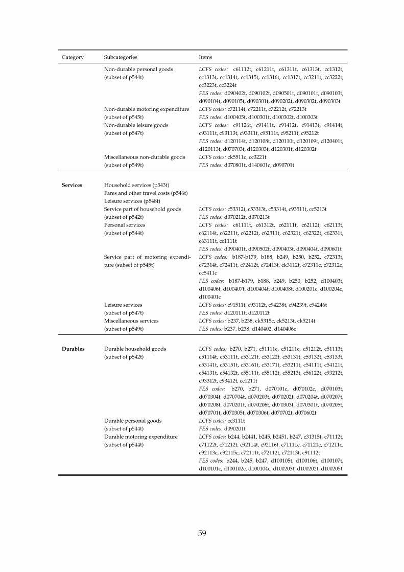
Category Subcategories Items

Non-durable personal goods(subset of p544t)

LCFS codes: c61112t, c61211t, c61311t, c61313t, cc1312t,cc1313t, cc1314t, cc1315t, cc1316t, cc1317t, cc3211t, cc3222t,cc3223t, cc3224tFES codes: d090402t, d090102t, d090501t, d090101t, d090103t,d090104t, d090105t, d090301t, d090202t, d090302t, d090303t

Non-durable motoring expenditure(subset of p545t)

LCFS codes: c72114t, c72211t, c72212t, c72213tFES codes: d100405t, d100301t, d100302t, d100303t

Non-durable leisure goods(subset of p547t)

LCFS codes: c91126t, c91411t, c91412t, c91413t, c91414t,c93111t, c93113t, c93311t, c95111t, c95211t, c95212tFES codes: d120114t, d120108t, d120110t, d120109t, d120401t,d120113t, d070703t, d120303t, d120301t, d120302t

Miscellaneous non-durable goods(subset of p549t)

LCFS codes: ck5511c, cc3221tFES codes: d070801t, d140601c, d090701t

Services Household services (p543t)Fares and other travel costs (p546t)Leisure services (p548t)Service part of household goods(subset of p542t)

LCFS codes: c53312t, c53313t, c53314t, c93511t, cc5213tFES codes: d070212t, d070213t

Personal services(subset of p544t)

LCFS codes: c61111t, c61312t, c62111t, c62112t, c62113t,c62114t, c62211t, c62212t, c62311t, c62321t, c62322t, c62331t,c63111t, cc1111tFES codes: d090401t, d090502t, d090403t, d090404t, d090601t

Service part of motoring expendi-ture (subset of p545t)

LCFS codes: b187-b179, b188, b249, b250, b252, c72313t,c72314t, c72411t, c72412t, c72413t, ck3112t, c72311c, c72312c,cc5411cFES codes: b187-b179, b188, b249, b250, b252, d100403t,d100406t, d100407t, d100404t, d100408t, d100201c, d100204c,d100401c

Leisure services(subset of p547t)

LCFS codes: c91511t, c93112t, c94238t, c94239t, c94246tFES codes: d120111t, d120112t

Miscellaneous services(subset of p549t)

LCFS codes: b237, b238, ck5315c, ck5213t, ck5214tFES codes: b237, b238, d140402, d140406c

Durables Durable household goods(subset of p542t)

LCFS codes: b270, b271, c51111c, c51211c, c51212t, c51113t,c51114t, c53111t, c53121t, c53122t, c53131t, c53132t, c53133t,c53141t, c53151t, c53161t, c53171t, c53211t, c54111t, c54121t,c54131t, c54132t, c55111t, c55112t, c55213t, c56122t, c93212t,c93312t, c93412t, cc1211tFES codes: b270, b271, d070101c, d070102c, d070103t,d070304t, d070704t, d070203t, d070202t, d070204t, d070207t,d070208t, d070201t, d070206t, d070303t, d070301t, d070205t,d070701t, d070305t, d070306t, d070702t, d070602t

Durable personal goods(subset of p544t)

LCFS codes: cc3111tFES codes: d090201t

Durable motoring expenditure(subset of p544t)

LCFS codes: b244, b2441, b245, b2451, b247, c31315t, c71112t,c71122t, c71212t, c92114t, c92116t, c71111c, c71121c, c71211c,c92113c, c92115c, c72111t, c72112t, c72113t, c91112tFES codes: b244, b245, b247, d100105t, d100106t, d100107t,d100101c, d100102c, d100104c, d100203t, d100202t, d100205t

59

Category Subcategories Items

Durable leisure goods(subset of p547t)

LCFS codes: c91124t, c82111t, c82112t, c82113t, c91111t,c91113t, c91121t, c91122t, c91123t, c91125t, c91211t, c91311t,c92211t, c92221t, c93211tFES codes: d120104t, d080202t, d080205t, d080207t, d120105t,d120101t, d120102t, d120103t, d120115t, d120402t, d120106t,d120107t, d120201t

Regarding the sample, I apply the following restrictions. I drop householdsthat have a household reference person younger than 18 or older than 90 years.Furthermore, I drop households with a negative normal disposable income. Toaccount for some (unrealistically) high or low values of consumption, for eachquarter and income group, I drop the top and bottom 1% of observations for totalexpenditure.

A.3.2. LFS

To get information on the sector of employment, I use data from the UK LabourForce Survey (LFS). The LFS studies the employment circumstances of the UKpopulation. It is the largest household study in the UK and provides the officialmeasures of employment and unemployment. Apart from detailed informationon employment, it also contains a wide range of related topics such as occupation,training, hours of work and personal characteristics of household members aged16 years and over. The data can be obtained from the UK Data Service. I usethe quarterly waves from 1999-2018 to construct a pooled cross-section. For theemployment sector, I use the variable indsect, which describes the industry sectorin the main job based on the SIC 2003 classification. To proxy income, I use thenet pay from the main and second job (netwk and netwk2).

A.3.3. BSA

To proxy public attitudes towards climate policy, I use data from the British socialattitudes (BSA) survey. The data can also be obtained from the UK Data Service. Iuse the waves from 1999-2018 to construct a pooled cross-section. To construct theincome groups, I use the income quartiles that are provided from 2010 onwards(hhincq). For the years before, I use the household income variable (hhincome)to construct the quartiles. The survey contains many questions on the attitudestowards climate change, the environment and climate/environmental policy, butunfortunately most variables are not part of the main set of questions that areasked in every year. One exception concerns a question about taxes for car owners(cartaxhi), in particular it asks whether you agree with the following statement:

60

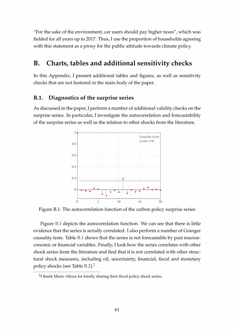
“For the sake of the environment, car users should pay higher taxes”, which wasfielded for all years up to 2017. Thus, I use the proportion of households agreeingwith this statement as a proxy for the public attitude towards climate policy.

B. Charts, tables and additional sensitivity checks

In this Appendix, I present additional tables and figures, as well as sensitivitychecks that are not featured in the main body of the paper.

B.1. Diagnostics of the surprise series

As discussed in the paper, I perform a number of additional validity checks on thesurprise series. In particular, I investigate the autocorrelation and forecastabilityof the surprise series as well as the relation to other shocks from the literature.

Figure B.1: The autocorrelation function of the carbon policy surprise series

Figure B.1 depicts the autocorrelation function. We can see that there is littleevidence that the series is serially correlated. I also perform a number of Grangercausality tests. Table B.1 shows that the series is not forecastable by past macroe-conomic or financial variables. Finally, I look how the series correlates with othershock series from the literature and find that it is not correlated with other struc-tural shock measures, including oil, uncertainty, financial, fiscal and monetarypolicy shocks (see Table B.2).2

2I thank Mario Alloza for kindly sharing their fiscal policy shock series.

61

Table B.1: Granger causality tests

Variable p-value

Instrument 0.9066EUA price 0.7575HICP energy 0.7551GHG emissions 0.7993HICP 0.8125Industrial production 0.7540Policy rate 0.9414Unemployment rate 0.9310Stock prices 0.9718REER 0.9075Joint 0.9997

Notes: The table shows the p-values of a series of Granger causality tests of the carbonpolicy surprise series using a selection of macroeconomic and financial variables.

Table B.2: Correlation with other shock measures

Shock Source ρ p-value n Sample

Monthly measuresGlobal oil marketOil supply Kilian (2008) (extended) -0.05 0.61 104 2005M05-2013M12

Kilian (2009) (updated) -0.02 0.76 164 2005M05-2018M12Caldara, Cavallo, and Iacoviello (2019) -0.05 0.57 128 2005M05-2015M12Baumeister and Hamilton (2019) -0.11 0.17 164 2005M05-2018M12Känzig (2021) (updated) 0.02 0.83 164 2005M05-2018M12

Global demand Kilian (2009) (updated) 0.01 0.93 164 2005M05-2018M12Baumeister and Hamilton (2019) -0.03 0.69 164 2005M05-2018M12

Oil-specific demand Kilian (2009) (updated) 0.05 0.55 164 2005M05-2018M12Consumption demand Baumeister and Hamilton (2019) 0.05 0.51 164 2005M05-2018M12Inventory demand Baumeister and Hamilton (2019) -0.03 0.68 164 2005M05-2018M12

Monetary policyMonetary policy shock Jarocinski and Karadi (2020) 0.02 0.80 140 2005M05-2016M12Central bank info Jarocinski and Karadi (2020) 0.03 0.75 140 2005M05-2016M12

Financial & uncertaintyFinancial conditions BBB spread residual 0.06 0.43 164 2005M05-2018M12Financial uncertainty VIX residual (Bloom, 2009) 0.10 0.22 164 2005M05-2018M12

VSTOXX residual 0.05 0.50 164 2005M05-2018M12Policy uncertainty Global EPU (Baker, Bloom, and Davis, 2016) 0.03 0.71 164 2005M05-2018M12

Quarterly measuresFiscal policy Euro area (Alloza, Burriel, and Pérez, 2019) 0.12 0.44 43 2005Q2-2015Q4

Germany 0.22 0.15 43 2005Q2-2015Q4France -0.06 0.69 43 2005Q2-2015Q4Italy 0.28 0.07 43 2005Q2-2015Q4Spain 0.10 0.52 43 2005Q2-2015Q4

Notes: The table shows the correlation of the carbon policy surprise series with a widerange of different shock measures from the literature, including global oil market shocks,monetary policy, financial and uncertainty shocks. ρ is the Pearson correlation coefficient,the p-value corresponds to the test whether the correlation is different from zero and n isthe sample size.

62

B.2. More on aggregate effects

In this Appendix, I present some additional results pertaining to the analysis inSection 5 in the paper.

B.2.1. Internal instrument approach

A key advantage of the external instruments approach lies in its efficiency. How-ever, this comes at the cost of assuming (partial) invertibility. If the invertibilityassumption is not satisfied, this can lead to biased results (Li, Plagborg-Møller,and Wolf, 2021). To mitigate concerns about invertibility, I also present resultsfrom the internal instruments approach (Ramey, 2011; Plagborg-Møller and Wolf,2019) which is robust to non-invertibility.

The results are shown in Figure B.2. The figure shows the responses from theinternal instrument approach together with the external instrument baseline. Wecan see that the responses turn out to be very similar, at least qualitatively. Thesigns are all consistent and the responses are also similar in shape. The maindifference lies in the response of energy prices, which turns out to be strongerand more persistent than in the external instrument model. Consequently, themagnitudes for emissions and the economic variables also turn out to be larger.Overall, however, these findings suggest that the results are robust to relaxing theassumption of invertibility. We can also see that the internal instrument responsesare much less precisely estimated as the confidence bands are significantly moredispersed.

B.2.2. Local projection-instrumental variable approach

As discussed in the main text, I rely on VAR techniques for estimation becausethe sample is relatively short and VARs provide a parsimonious characterizationof the data. However, as a robustness check, I have also tried to estimate the im-pulse responses using a local projections instrumental variable (LP-IV) approachà la Jordà, Schularick, and Taylor (2015) and Ramey and Zubairy (2018). To fixideas, the dynamic causal effects, ψi

h, can be estimated from the following set ofregressions:

yi,t+h − yi,t−1 = βih + ψi

h∆y1,t + βi′hxt−1 + ξi,t,h, (1)

using zt as an instrument for ∆y1,t. Here, yi,t+h is the outcome variable of interest,∆y1,t is the endogenous regressor, xt−1 is a vector of controls, ξi,t,h is a potentiallyserially correlated error term, and h is the impulse response horizon. For infer-

63

Figure B.2: Internal versus external instrument VAR

Notes: Impulse responses to a carbon policy shock, normalized to increase the HICPenergy by 1 percent on impact. The solid dark and red lines are the point estimates forthe internal instrument and the external instrument VAR, respectively, and the shadedareas / dashed lines are 68 and 90 percent confidence bands.

64

Figure B.3: Internal instrument VAR versus LP-IV

Notes: Impulse responses to a carbon policy shock, normalized to increase the HICPenergy by 1 percent on impact. The solid dark and red lines are the point estimates forthe internal instrument VAR and the LP-IV, respectively, and the shaded areas / dashedlines are 68 and 90 percent confidence bands.

65

ence, I follow again the lag-augmentation approach proposed by Montiel Oleaand Plagborg-Møller (2020).

As the impacts of carbon policy are potentially very persistent, we want tolook at the dynamic causal effects relatively far out. Given the short sample, thisis challenging in the LP-IV framework, which does not use the parametric VARrestriction but estimates the effect by a distinct IV regression at each horizon h.Consequently, the number of observations available for estimation decreases withthe impulse horizon. Against this background, I restrict the impulse horizon inthe LP-IV regressions to 20 months.

Figure B.3 compares the responses obtained from the LP-IV approach to theones from the internal instrument VAR. Recall that both approaches rely onthe same invertibility-robust identifying restrictions but use different estimationtechniques. We can see that the two approaches produce consistent results, espe-cially at horizons up to one year.3 At longer horizons the differences tend to belarger, however, the responses are also much less precisely estimated.

B.2.3. Core versus headline HICP

In the paper, I document a significant and persistent increase in headline HICP.An important question that has also relevant implications for the conduct of mon-etary policy is how the shock transmits to core consumer prices. To this end, I re-estimate the model substituting headline for core HICP. Figure B.4 presents theresponse for core HICP together with the HICP headline and energy componentfrom the baseline model. We can see that the response of core consumer pricesis more muted and much less precisely estimated. Importantly, the response alsoturns out to be much less persistent, which may reflect the fact that the fall ineconomic activity exerts downward pressure on prices other than energy, suchas services. Reassuringly, all other responses from the model with core HICP arevery similar to the baseline case.

3Note that this is despite the fact that we only control for 6 lags in both models.

66

Figure B.4: Headline versus core HICP

Notes: Impulse responses of the headline, energy and core HICP to a carbon policy shock.The headline and energy indices are from the baseline model; the core response is fromthe model featuring core instead of headline HICP. The solid line is the point estimateand the dark and light shaded areas are 68 and 90 percent confidence bands, respectively.

B.2.4. Model with carbon price

Recall, the baseline model does not include the carbon price as information onprices is only available from 2005 when the carbon market was established. As arobustness check, I estimate a model including the carbon price in lieu of GHGemissions on the shorter sample starting from 2005. The results are depicted inFigure B.5. We can see that the shock leads to a significant increase in the car-bon price, in line with the interpretation of a shock tightening the carbon pricingregime. Interestingly, however, the carbon price response turns out to be lesspersistent than the energy price response. We can also back out the elasticity ofenergy to carbon prices, which turns out to be around 20 percent at the peak.

67

Figure B.5: Model including carbon spot price

Notes: Impulse responses to a carbon policy shock, normalized to increase the HICPenergy by 1 percent on impact. The solid line is the point estimate and the dark and lightshaded areas are 68 and 90 percent confidence bands, respectively.

B.2.5. Variance decomposition

To better understand how carbon policy shocks have contributed to variationsin macroeconomic and financial variables, I perform a variance decompositionin addition to the historical decomposition presented in the paper. I do so bothunder the invertibility assumption maintained in the external instrument VAR aswell as under weaker assumptions in the context of a general SVMA model, asproposed by Plagborg-Møller and Wolf (2020). In particular, I perform a standard

68

forecast error variance decomposition in the SVAR and compute forecast varianceratios for the SVMA. The forecast variance ratio for variable i at horizon h is givenby

FVRi,h = 1− Var(yi,t+h|yτ−∞<τ≤t, ε1,τt<τ<∞)

Var(yi,t+h|yτ−∞<τ≤t), (2)

and measures the reduction in the econometrician’s forecast variance that wouldarise from being told the entire path of future realizations of the shock of interest.Plagborg-Møller and Wolf (2020) show that this statistic is interval-identified un-der the assumption that a valid instrument is available. Under the assumption ofrecoverablity, the ratio is point-identified by the upper bound.

The results are shown in Table B.3. We can see that carbon policy shocks havecontributed meaningfully to historical variations in the variables of interest. Un-der the invertibility assumption (Panel A), they account for about 40 percent ofthe variations in energy prices and around 10 percent of the short-run variationsin emissions, which goes up to almost 40 percent at the 5 year horizon. Turningto the macroeconomic variables, we can see that they explain a substantial partof variations in the HICP, especially at shorter horizons, and a significant fractionof the variations in industrial production and the unemployment rate at longerhorizons. The contributions to variations in the policy rate, stock prices and theREER are lower but still non-negligible.

The forecast variance ratios in Panel B, which dispense from the assumptionof invertibility, paint a slightly more nuanced picture. In many cases, the pointestimates from the external instrument VAR lie within the estimated intervals.The largest differences arise for the contributions to stock prices and the REERwhich are estimated to be significantly lower when allowing for non-invertibility.However, overall the two approaches produce comparable results.

69

Table B.3: Variance decomposition

h HICP energy Emissions HICP IP Policy rate Unemp. rate Stock prices REER

Panel A: Forecast variance decomposition (SVAR-IV)6 0.41 0.12 0.49 0.02 0.00 0.07 0.12 0.00

[0.20, 0.81] [0.03, 0.41] [0.27, 0.83] [0.00, 0.07] [0.00, 0.01] [0.01, 0.55] [0.03, 0.63] [0.00, 0.01]12 0.34 0.25 0.34 0.14 0.03 0.23 0.15 0.00

[0.14, 0.71] [0.07, 0.69] [0.15, 0.68] [0.04, 0.49] [0.01, 0.19] [0.06, 0.84] [0.04, 0.65] [0.00, 0.01]24 0.35 0.33 0.25 0.27 0.12 0.37 0.11 0.08

[0.15, 0.70] [0.10, 0.73] [0.08, 0.54] [0.09, 0.67] [0.03, 0.54] [0.12, 0.91] [0.03, 0.48] [0.03, 0.26]48 0.39 0.34 0.19 0.22 0.12 0.39 0.11 0.20

[0.16, 0.72] [0.13, 0.68] [0.05, 0.47] [0.08, 0.57] [0.03, 0.46] [0.13, 0.85] [0.03, 0.45] [0.06, 0.48]

Forecast variance ratio (SVMA-IV)6 0.04, 0.31 0.02, 0.18 0.07, 0.49 0.02, 0.14 0.00, 0.02 0.05, 0.35 0.00, 0.03 0.00, 0.00

[0.02, 0.53] [0.01, 0.40] [0.04, 0.75] [0.01, 0.34] [0.00, 0.06] [0.03, 0.59] [0.00, 0.09] [0.00, 0.02]12 0.05, 0.33 0.03, 0.18 0.07, 0.50 0.02, 0.16 0.00, 0.02 0.05, 0.36 0.01, 0.04 0.00, 0.01

[0.03, 0.53] [0.01, 0.36] [0.04, 0.73] [0.01, 0.33] [0.00, 0.05] [0.03, 0.60] [0.00, 0.08] [0.00, 0.02]24 0.05, 0.32 0.03, 0.19 0.07, 0.50 0.02, 0.18 0.01, 0.08 0.08, 0.54 0.01, 0.04 0.00, 0.01

[0.02, 0.51] [0.01, 0.36] [0.04, 0.72] [0.01, 0.35] [0.01, 0.19] [0.04, 0.78] [0.00, 0.09] [0.00, 0.02]48 0.05, 0.32 0.03, 0.19 0.07, 0.50 0.02, 0.18 0.01, 0.08 0.09, 0.55 0.01, 0.05 0.00, 0.01

[0.02, 0.51] [0.01, 0.35] [0.04, 0.72] [0.01, 0.34] [0.01, 0.19] [0.04, 0.78] [0.00, 0.09] [0.00, 0.02]

Notes: The table shows variance decomposition at horizons ranging from 6 months to4 years. Panel A includes the forecast error variance decomposition from the externalinstrument VAR with the point estimates and the 90% confidence interval in brackets.Panel B shows the identified set for the forecast variance ratio together with the 90%confidence interval in brackets.

B.2.6. Financial conditions and uncertainty

To better understand how the shock transmits to the economy, I have also lookedat the responses of indicators for financing conditions and financial uncertainty,see Figure B.6. However, as can be seen from the responses these variables do notappear to play a dominant role in the transmission of the carbon policy shock.

Figure B.6: Financial and uncertainty indicatorsNotes: Impulse responses of financial conditions, as proxied by the BBB bond spread,and the VSTOXX index as a measure of financial uncertainty.

B.2.7. Aggregate effects for the UK

Because of data availability, the household-level analysis is carried out for theUK. As a validating exercise, I have verified that the aggregate effects on the UK,

70

as measured by real GDP, consumption and investment, are comparable to theEU level responses, see Figure B.7.

Figure B.7: Effect on UK GDP and components

Notes: Impulse responses of UK real GDP, consumption, investment and net exportsexpressed as a share of GDP.

B.3. More on heterogeneous effects

In this Appendix, I present some additional results pertaining to Section 6 on theheterogeneous effects of carbon pricing in the paper.

B.3.1. Further descriptive statistics

Figure B.8 compares the empirical distribution of age and total expenditure forthe three income groups. We can see that the groups are comparable in terms oftheir age distribution. As expected, higher income groups tend to have higherexpenditure but there is also more within group variation.

71

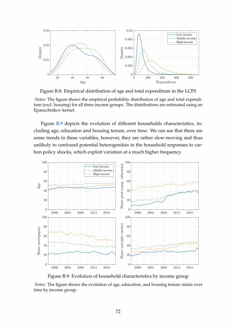
Figure B.8: Empirical distribution of age and total expenditure in the LCFS

Notes: The figure shows the empirical probability distribution of age and total expendi-ture (excl. housing) for all three income groups. The distributions are estimated using anEpanechnikov kernel.

Figure B.9 depicts the evolution of different households characteristics, in-cluding age, education and housing tenure, over time. We can see that there aresome trends in these variables, however, they are rather slow-moving and thusunlikely to confound potential heterogenities in the household responses to car-bon policy shocks, which exploit variation at a much higher frequency.

Figure B.9: Evolution of household characteristics by income group

Notes: The figure shows the evolution of age, education, and housing tenure status overtime by income group.

72

B.3.2. Aggregate expenditure responses

Before studying at the heterogeneous expenditure responses by income group, Ilook at the aggregate expenditure responses as a validating exercise. The resultsare shown in Figures B.10-B.11. We can see that the response of aggregated ex-penditure from household micro data is very similar to the consumption responsefrom national statistics – both in terms of shape and magnitude. This supportsthe notion that the micro data is indeed representative for the macroeconomy.

Figure B.10: Responses of total expenditure

Figure B.11: Responses of non-durable and durable expenditure

B.3.3. Energy expenditure and share responses

In the main text, we have seen that energy bills increase substantially across allhouseholds. However, energy bills are measured in nominal terms, deflated bythe headline HICP. It is also interesting to look at the response of real energyexpenditure, i.e. energy bills deflated by the energy HICP. These responses areshown in Figure B.12, together with the response of the energy share (i.e. en-ergy expenditure as a share of total expenditure). We can see that real energyexpenditure falls significantly for about one year and is insignificant after. Theenergy share on the other hand has a tendency to increase, which reflects the sig-nificant fall in non-energy expenditure together with the inelastic response of en-ergy expenditure. Figure B.13 further presents the energy expenditure responses

73

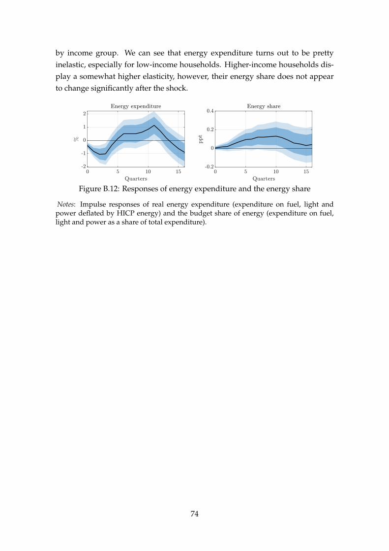
by income group. We can see that energy expenditure turns out to be prettyinelastic, especially for low-income households. Higher-income households dis-play a somewhat higher elasticity, however, their energy share does not appearto change significantly after the shock.

Figure B.12: Responses of energy expenditure and the energy share

Notes: Impulse responses of real energy expenditure (expenditure on fuel, light andpower deflated by HICP energy) and the budget share of energy (expenditure on fuel,light and power as a share of total expenditure).

74

Figure B.13: Energy expenditure and energy share by income group

Notes: Impulse responses of real energy expenditure and the budget share of energy byincome group (bottom 25 percent, middle 50 percent, top 25 percent).

B.3.4. Smoothing impulse responses

In the LCFS, households interviewed at time t are typically asked to report ex-penditure over the previous three months (with the exception of non-durableconsumption which refers to the previous two weeks). To eliminate some of thenoise inherent in survey data, I smooth the expenditure and income measureswith a backward-looking (current and previous three quarters) moving average,as in Cloyne, Ferreira, and Surico (2020). However, as shown in Figure B.14, theresults are very similar when using the raw series instead, even though the re-sponses become more jagged and imprecise, or by using smooth local projectionsas proposed by Barnichon and Brownlees (2019).

75

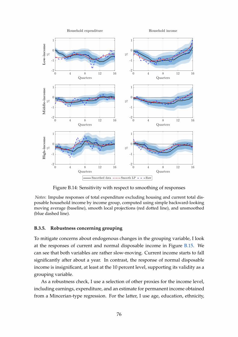
Figure B.14: Sensitivity with respect to smoothing of responses

Notes: Impulse responses of total expenditure excluding housing and current total dis-posable household income by income group, computed using simple backward-lookingmoving average (baseline), smooth local projections (red dotted line), and unsmoothed(blue dashed line).

B.3.5. Robustness concerning grouping

To mitigate concerns about endogenous changes in the grouping variable, I lookat the responses of current and normal disposable income in Figure B.15. Wecan see that both variables are rather slow-moving. Current income starts to fallsignificantly after about a year. In contrast, the response of normal disposableincome is insignificant, at least at the 10 percent level, supporting its validity as agrouping variable.

As a robustness check, I use a selection of other proxies for the income level,including earnings, expenditure, and an estimate for permanent income obtainedfrom a Mincerian-type regression. For the latter, I use age, education, ethnicity,

76

Figure B.15: Responses of current and normal income

Notes: Impulse responses of current disposable income and normal disposable income.

sex, martial status, occupation, the source of the main household income, as wellas interactions between age and education, and between age and sex as predic-tors, as in Alves et al. (2020). From Figures B.16-B.18, we can see that the resultsturn out to be robust.

77

Figure B.16: Expenditure and income responses by earnings groups

Notes: Impulse responses of total expenditure excluding housing and current total dis-posable household income by earnings (incl. benefits) groups (bottom 25 percent, middle50 percent, top 25 percent).

78

Figure B.17: Expenditure and income responses by expenditure groups

Notes: Impulse responses of total expenditure excluding housing and current total dis-posable household income by groups of total expenditure as a proxy for permanent in-come (bottom 25 percent, middle 50 percent, top 25 percent).

79

Figure B.18: Expenditure and income responses by permanent income

Notes: Impulse responses of total expenditure excluding housing and current total dis-posable household income by permanent income, estimated using a Mincerian-type re-gression using age, education, ethnicity, sex, martial status, occupation, the source of themain household income, as well as interactions between age and education, and betweenage and sex (bottom 25 percent, middle 50 percent, top 25 percent).

B.3.6. Selection

To mitigate concerns about selection, I use a number of different grouping vari-ables, including age, education and housing tenure. From Figures B.19-B.21, wecan see that none of these alternative grouping variables can account for the pat-terns uncovered for income, suggesting that we are not spuriously picking updifferences in other household characteristics. Similarly, the uncovered hetero-geneity can also not be accounted for by occupation, sex and region. These resultsare available from the author upon request.

80

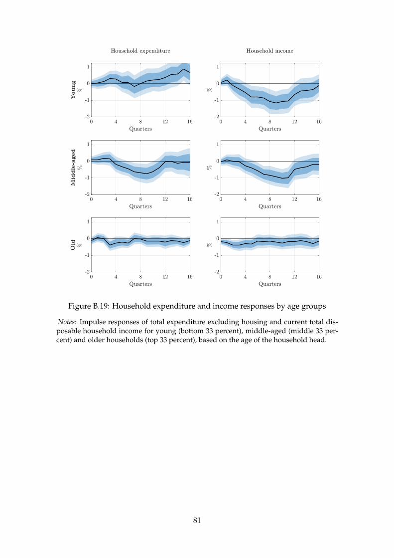
Figure B.19: Household expenditure and income responses by age groups

Notes: Impulse responses of total expenditure excluding housing and current total dis-posable household income for young (bottom 33 percent), middle-aged (middle 33 per-cent) and older households (top 33 percent), based on the age of the household head.

81

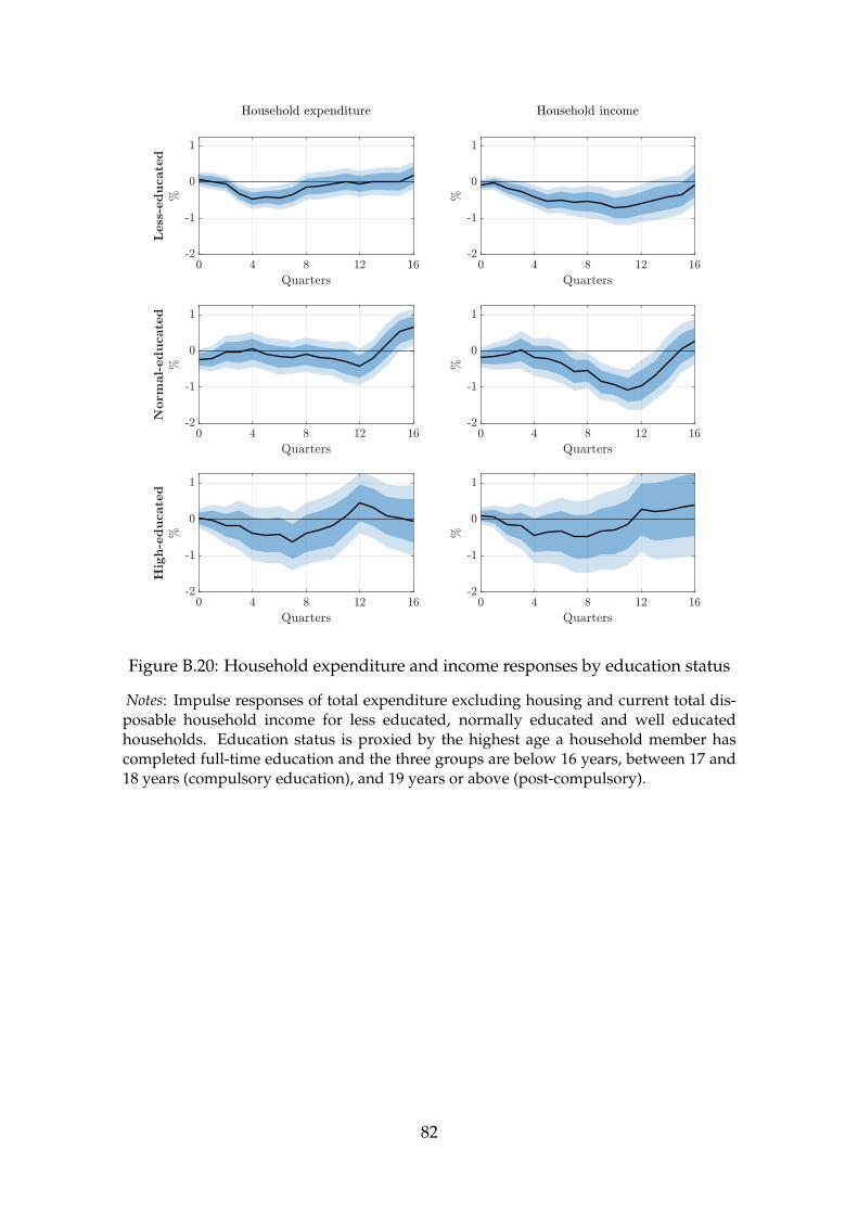
Figure B.20: Household expenditure and income responses by education status

Notes: Impulse responses of total expenditure excluding housing and current total dis-posable household income for less educated, normally educated and well educatedhouseholds. Education status is proxied by the highest age a household member hascompleted full-time education and the three groups are below 16 years, between 17 and18 years (compulsory education), and 19 years or above (post-compulsory).

82

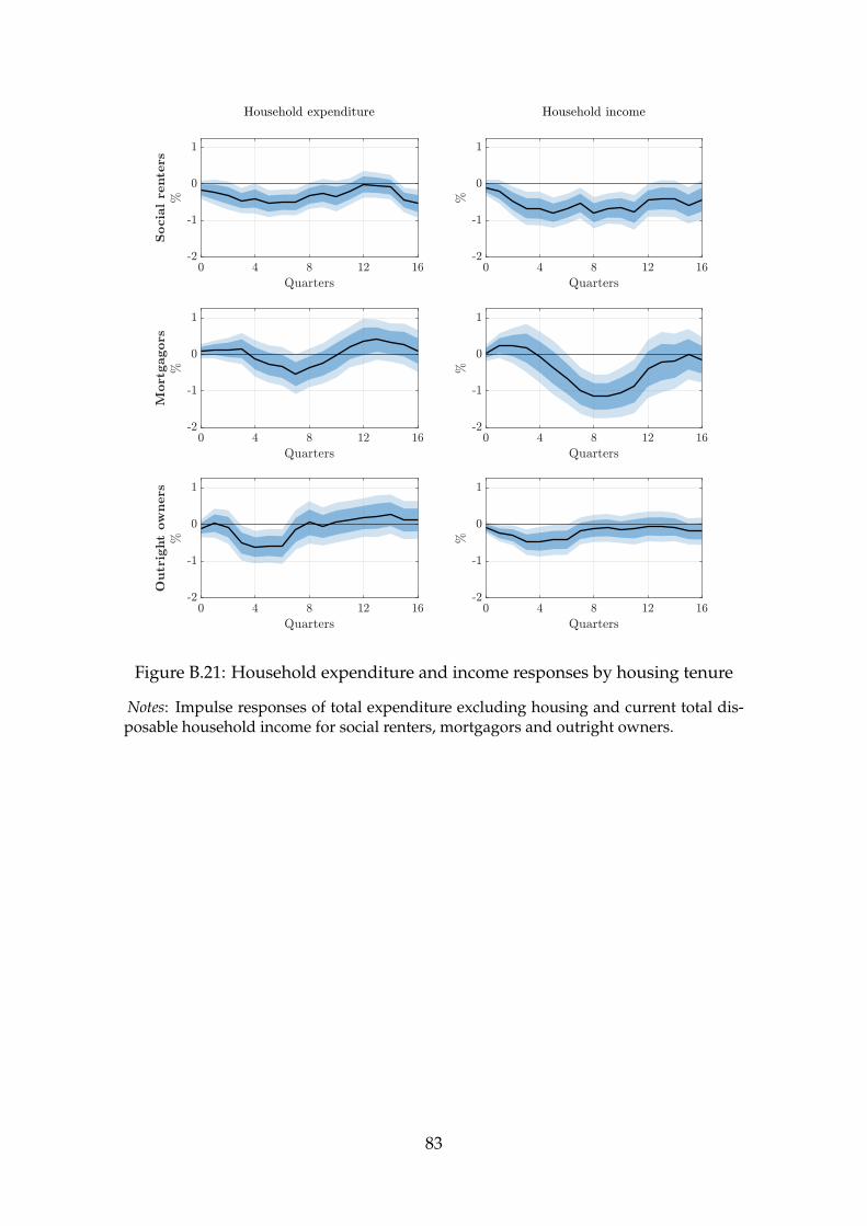
Figure B.21: Household expenditure and income responses by housing tenure

Notes: Impulse responses of total expenditure excluding housing and current total dis-posable household income for social renters, mortgagors and outright owners.

83

B.3.7. Grouping by energy share

A key difference between high- and low-income households concerns their en-ergy share. Furthermore, the energy share turns out to be relatively unresponsive,in line with the notion that energy demand is relatively inelastic and improvingthe energy efficiency may not be feasible or take some time. This suggests that theenergy share may be an alternative grouping variable of interest. To analyze this,I alternatively group households by their energy share, i.e. households with ahigh energy share, households with a normal energy share, and households witha low energy share.

The corresponding expenditure and income responses are shown in FigureB.22. We can see that the magnitude of the expenditure response is clearly in-creasing in the energy share: while the expenditure of households with a highenergy share falls significantly and persistently, households with a low energyshare barely alter their expenditure. However, there is also again significant het-erogeneity in the income responses, with the high energy share households expe-riencing the strongest fall in their income.

84

Figure B.22: Household expenditure and income responses by energy share

Notes: Impulse responses of total expenditure excluding housing and current total dis-posable household income for households with a high energy share (top 25 percent), atypical energy share (middle 50 percent) and low energy share (bottom 25 percent). Theenergy share is measured as expenditure on fuel, light and power, as a share of total ex-penditure excluding housing and the responses are computed based on the median ofthe respective group.

An explanation for this finding is that high energy share households also tendto be poorer and thus have more cyclical income for reasons dicussed in the maintext. This is confirmed by looking at descriptive statistics on income, expenditureand other characteristics by the households’ energy share. As can be seen fromTable B.4, household income and expenditure turns out to be decreasing in theenergy share. Furthermore, the high-, middle- and low-energy share groups turnout to be comparable to the low-, middle- and high-income groups along manydimensions. The largest differences are that high-energy share households tendto be older and more likely to be homeowners than households in the low-incomegroup. Overall, these results confirm that the energy share can be used as a proxy

85

for the income-level.

Table B.4: Descriptive statistics on households in the LCFS

Overall By energy share

High-share Middle-share Low-share

Income and expenditureNormal disposable income 6,699 3,975 7,347 9,061Total expenditure 4,459 2,109 4,955 7,677

Energy share 7.2 15.9 5.5 1.8Non-durables (excl. energy) share 81.5 78.9 82.9 81.4Durables share 11.3 5.2 11.6 16.8

Household characteristicsAge 51 62 50 45Education (share with post-comp.) 33.5 17.8 35.3 45.7Housing tenure

Social renters 20.9 34.2 15.9 17.7Mortgagors 42.6 20.6 47.5 55.0Outright owners 36.6 45.3 36.6 27.3

Notes: The table shows descriptive statistics on quarterly household income and expen-diture (in 2015 pounds), the breakdown of expenditure into energy, non-durable goodsand services excl. energy, and durables (as a share of total expenditure) as well as a se-lection of household characteristics, both over all households and by energy share group.For variables in levels such as income, expenditure and age the median is shown whilethe shares are computed based on the mean of the corresponding variable. Note thatthe expenditure shares are expressed as a share of total expenditure excl. housing andsemi-durables are subsumed under the non-durable category. Age corresponds to theage of the household reference person and education is proxied by whether a householdmember has completed a post-compulsory education.

B.3.8. What drives the income response?

To understand what is driving the heterogeneity in the income responses, westudy how the labor income responses vary by sector of employment using datafrom the LFS. To this end, I grouped sectors by their energy intensity and theirdemand sensitivity based on information on SIC 2003 sections. A detailed de-scription of all the four groups can be found in Table B.5.

As explained in the main text, I have excluded utilities from the group ofenergy-intensive sectors when looking at the income response, as the utility sec-tor may respond very differently from other energy-intensive sectors. Indeed,as shown in Figure B.23, the households working in utilities do not experience asignificant change in their income, consistent the results from Section 5.4. Thisfurther supports the notion that the utility sector can, at least in the short run,profit from a more restrictive carbon pricing regime. In contrast, incomes in otherhigh-energy intensive sectors display a significant fall. However, the response

86

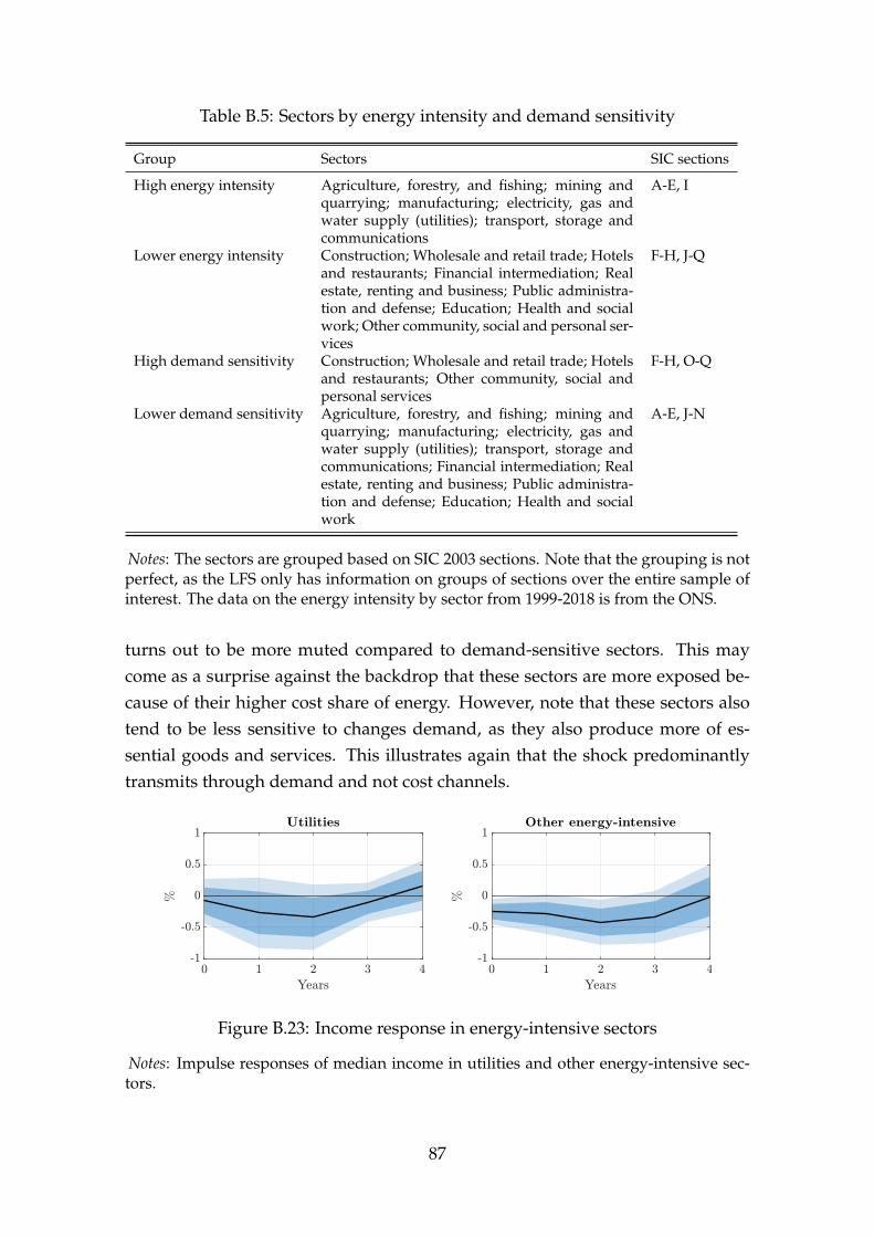
Table B.5: Sectors by energy intensity and demand sensitivity

Group Sectors SIC sections

High energy intensity Agriculture, forestry, and fishing; mining andquarrying; manufacturing; electricity, gas andwater supply (utilities); transport, storage andcommunications

A-E, I

Lower energy intensity Construction; Wholesale and retail trade; Hotelsand restaurants; Financial intermediation; Realestate, renting and business; Public administra-tion and defense; Education; Health and socialwork; Other community, social and personal ser-vices

F-H, J-Q

High demand sensitivity Construction; Wholesale and retail trade; Hotelsand restaurants; Other community, social andpersonal services

F-H, O-Q

Lower demand sensitivity Agriculture, forestry, and fishing; mining andquarrying; manufacturing; electricity, gas andwater supply (utilities); transport, storage andcommunications; Financial intermediation; Realestate, renting and business; Public administra-tion and defense; Education; Health and socialwork

A-E, J-N

Notes: The sectors are grouped based on SIC 2003 sections. Note that the grouping is notperfect, as the LFS only has information on groups of sections over the entire sample ofinterest. The data on the energy intensity by sector from 1999-2018 is from the ONS.

turns out to be more muted compared to demand-sensitive sectors. This maycome as a surprise against the backdrop that these sectors are more exposed be-cause of their higher cost share of energy. However, note that these sectors alsotend to be less sensitive to changes demand, as they also produce more of es-sential goods and services. This illustrates again that the shock predominantlytransmits through demand and not cost channels.

Figure B.23: Income response in energy-intensive sectors

Notes: Impulse responses of median income in utilities and other energy-intensive sec-tors.

87

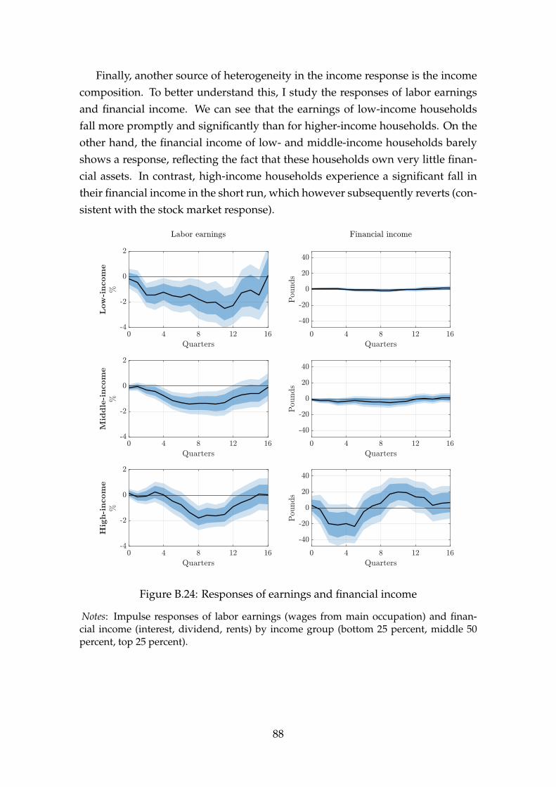
Finally, another source of heterogeneity in the income response is the incomecomposition. To better understand this, I study the responses of labor earningsand financial income. We can see that the earnings of low-income householdsfall more promptly and significantly than for higher-income households. On theother hand, the financial income of low- and middle-income households barelyshows a response, reflecting the fact that these households own very little finan-cial assets. In contrast, high-income households experience a significant fall intheir financial income in the short run, which however subsequently reverts (con-sistent with the stock market response).

Figure B.24: Responses of earnings and financial income

Notes: Impulse responses of labor earnings (wages from main occupation) and finan-cial income (interest, dividend, rents) by income group (bottom 25 percent, middle 50percent, top 25 percent).

88

B.3.9. External validity

To mitigate concerns regarding external validity, I confirm the main results on theheterogeneity in household expenditure by income group using data for Den-mark and Spain. As can be seen from Figure B.25, the expenditure responseturns out to be significant and persistent for low-income households, while high-income households are much less affected. These findings confirm the results forthe UK, supporting the external validity of the results.

Figure B.25: Expenditure by income groups for other European countries

Notes: Impulse responses of total expenditure for low-income, middle-income and high-income households in Denmark and Spain. The Danish data are from the Danish house-hold budget survey (HBS) available for 1999-2018, accessed via the StatBank Denmarkdatabase, and expenditure is grouped by total annual income (under 250K DKK, 250-999K DKK, 1000K DKK or over). The Spanish data are from the Spanish HBS availablefor 2006-2018, accessed via the INE website, and expenditure is grouped by regular netmonthly household income (under 1000 euros, 1000-2499 euros, 2500 euros or over).

89

B.3.10. Attitudes towards climate policy

As discussed in the paper, public opposition can be an impediment for climatepolicy. Thus, it is interesting to see how carbon pricing affects the public attitudetowards climate policy. To analyze this question, I use data from the British socialattitudes (BSA) survey. The BSA is an annual survey that asks about the attitudesof the British population towards a wide selection of topics, ranging from wel-fare to genomic science. The BSA is used to inform the development of publicpolicy and is an important barometer of public attitudes. Some of the questionsin the BSA are repeated over time and thus, it is possible to analyze how certainattitudes have changed over time.

To proxy the public attitude towards climate policy, I rely on a question fromthe transportation module of the survey, which asks about the attitude towardsfuel taxes. In particular, the question asks whether the respondent agrees withthe following statement: “For the sake of the environment, car users should payhigher taxes”. The BSA also includes information about the income of the re-spondent, thus it is possible to analyze how the attitudes of different incomegroups have evolved. Figure B.26 shows how the attitude towards fuel taxes haschanged among low- and higher-income households. We can see that the supportof climate policy has remained relatively stable at moderate levels for a large partof the sample. In the early to middle 2010s, the support started increasing forhigher-income households. In contrast, the support of low-income householdshas remained stable until the end of the sample.

Figure B.26: Public support for climate policy by income group

Notes: The figure shows the evolution of the attitude towards climate policy by incomegroup, as proxied by the share of households in the British social attitudes survey thatagree to the following statement: “For the sake of the environment, car users should payhigher taxes”.

90

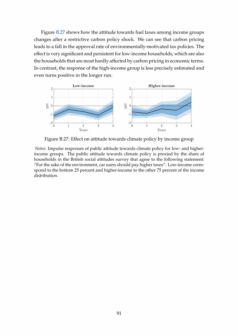
Figure B.27 shows how the attitude towards fuel taxes among income groupschanges after a restrictive carbon policy shock. We can see that carbon pricingleads to a fall in the approval rate of environmentally-motivated tax policies. Theeffect is very significant and persistent for low-income households, which are alsothe households that are most hardly affected by carbon pricing in economic terms.In contrast, the response of the high-income group is less precisely estimated andeven turns positive in the longer run.

Figure B.27: Effect on attitude towards climate policy by income group

Notes: Impulse responses of public attitude towards climate policy for low- and higher-income groups. The public attitude towards climate policy is proxied by the share ofhouseholds in the British social attitudes survey that agree to the following statement:“For the sake of the environment, car users should pay higher taxes”. Low-income corre-spond to the bottom 25 percent and higher-income to the other 75 percent of the incomedistribution.

91

B.4. Additional results from heterogeneous-agent climate-

economy model

In this appendix, we present some additional results from the heterogeneous-agent climate-economy model. Figure B.28 shows the response of emissionsunder the two carbon revenue redistribution schemes. We can see that emis-sions fall by somewhat less when redistributing revenues than under the base-line case when all revenues accrue to the savers but importantly, the consump-tion response is dampened significantly more. This suggests that there could bea trade-off that policy makers could exploit.

Figure B.28: Emissions response

As discussed in the main text, household heterogeneity is crucial in getting theempirical magnitudes of the consumption responses right. Without the hetero-geneity in MPCs, energy shares and income incidence, it is virtually infeasible toget the sizeable responses observed in the data without implausibly high firm andhousehold energy shares. This is illustrated in Figure B.29, which compares theresponses of the heterogeneous agent to the corresponding representative agentversion of the model.

92

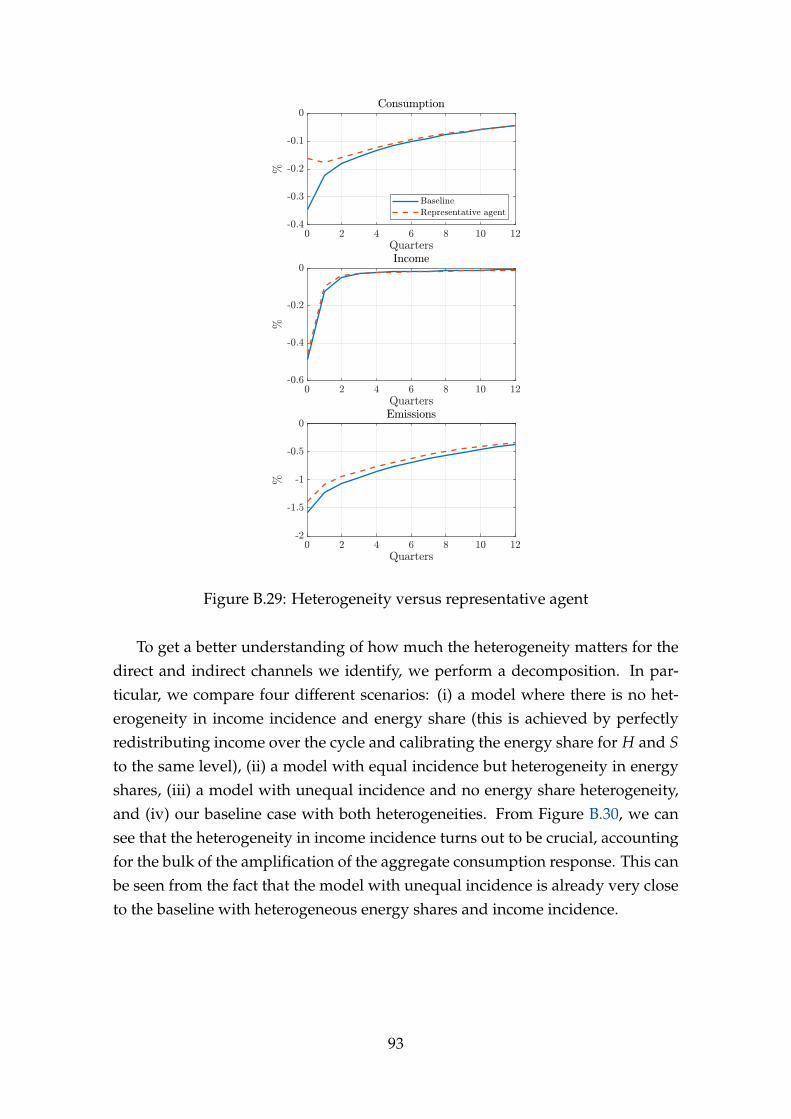
Figure B.29: Heterogeneity versus representative agent

To get a better understanding of how much the heterogeneity matters for thedirect and indirect channels we identify, we perform a decomposition. In par-ticular, we compare four different scenarios: (i) a model where there is no het-erogeneity in income incidence and energy share (this is achieved by perfectlyredistributing income over the cycle and calibrating the energy share for H and Sto the same level), (ii) a model with equal incidence but heterogeneity in energyshares, (iii) a model with unequal incidence and no energy share heterogeneity,and (iv) our baseline case with both heterogeneities. From Figure B.30, we cansee that the heterogeneity in income incidence turns out to be crucial, accountingfor the bulk of the amplification of the aggregate consumption response. This canbe seen from the fact that the model with unequal incidence is already very closeto the baseline with heterogeneous energy shares and income incidence.

93

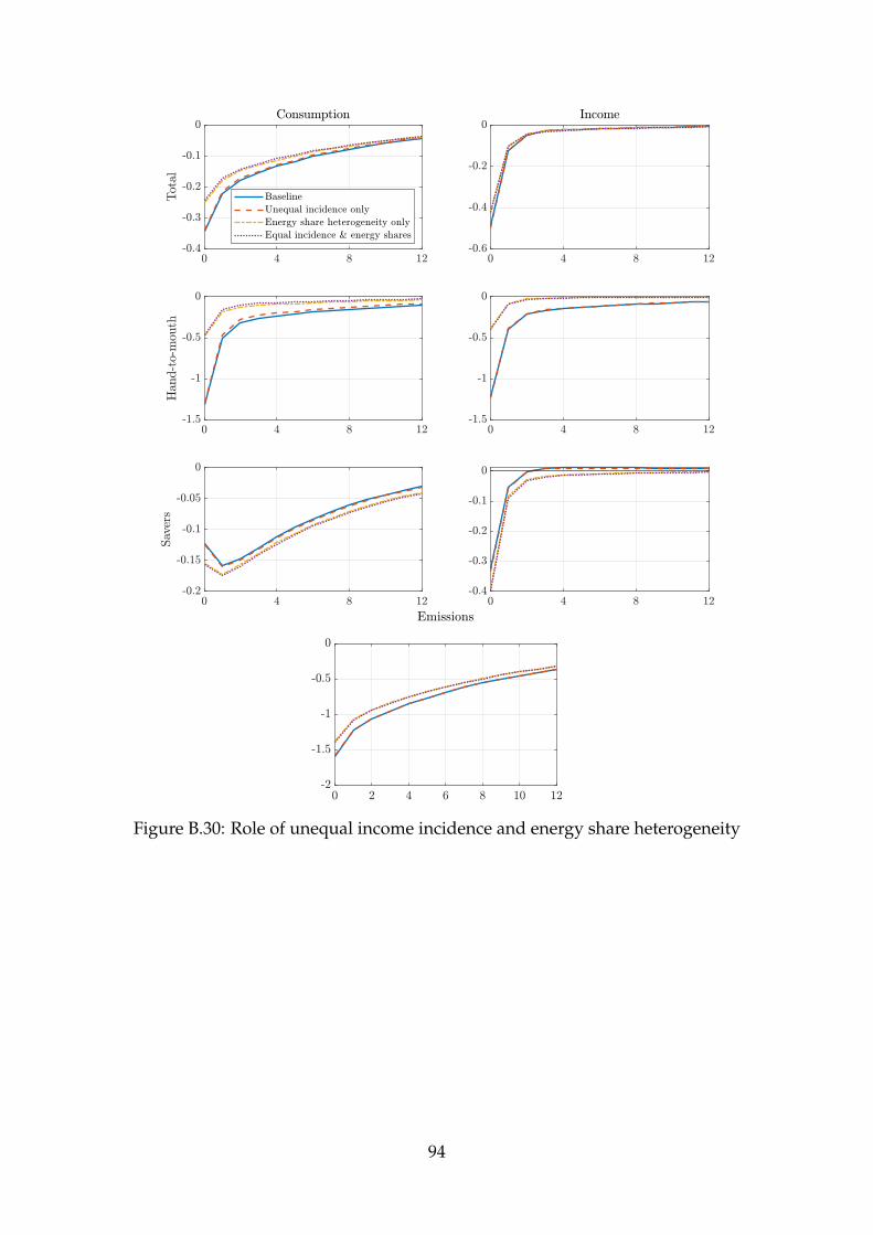
Figure B.30: Role of unequal income incidence and energy share heterogeneity

94

B.5. Robustness

In this Appendix, I present the Figures and Tables corresponding to the robust-ness analyses discussed in Section 8 of the paper.

B.5.1. Selection of events

The first check concerns the selection of the relevant events used for identifica-tion. As the baseline, I have included all identified events that concern the sup-ply of emission allowances. Figures B.31-B.34 present the results under varyingassumptions and show that the results turn out to be very robust to the selectionof events. Figure B.35 also shows that the identification strategy does not dependon very large events, even though these events turn out to be important for theprecision of the estimates.

95

Figure B.31: Excluding events regarding cap

Notes: Impulse responses to a carbon policy shock, normalized to increase the HICPenergy by 1 percent on impact. The solid line is the point estimate and the dark and lightshaded areas are 68 and 90 percent confidence bands, respectively.

96

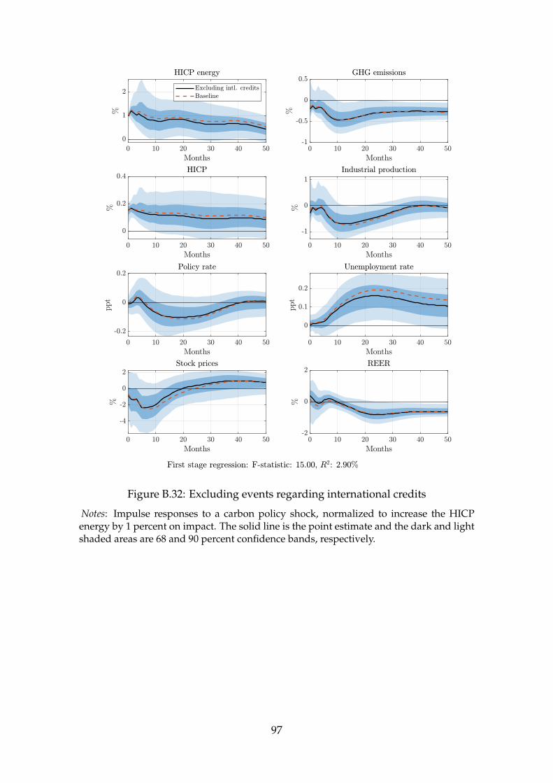
Figure B.32: Excluding events regarding international credits

Notes: Impulse responses to a carbon policy shock, normalized to increase the HICPenergy by 1 percent on impact. The solid line is the point estimate and the dark and lightshaded areas are 68 and 90 percent confidence bands, respectively.

97

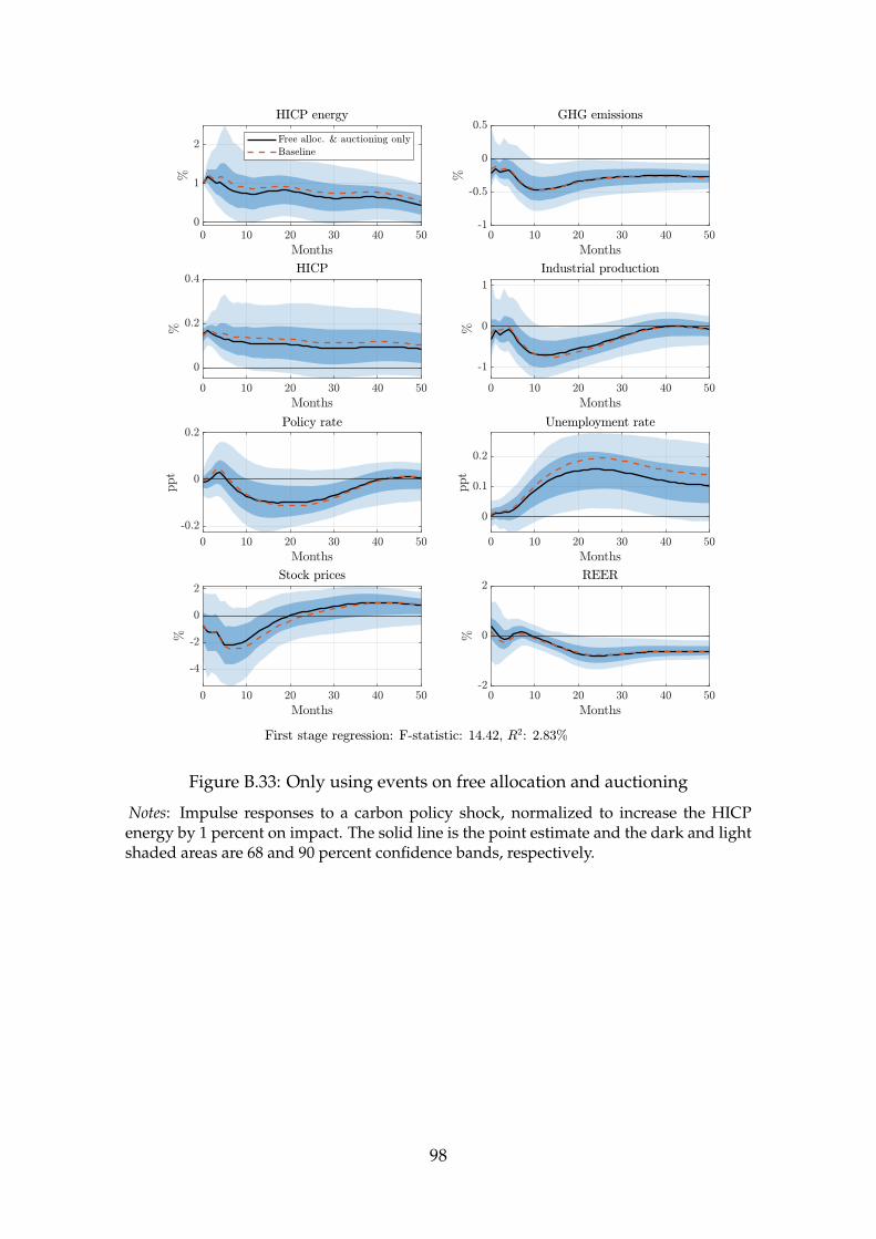
Figure B.33: Only using events on free allocation and auctioning

Notes: Impulse responses to a carbon policy shock, normalized to increase the HICPenergy by 1 percent on impact. The solid line is the point estimate and the dark and lightshaded areas are 68 and 90 percent confidence bands, respectively.

98

Figure B.34: Excluding potentially confounded events

Notes: Impulse responses to a carbon policy shock, normalized to increase the HICPenergy by 1 percent on impact. The solid line is the point estimate and the dark and lightshaded areas are 68 and 90 percent confidence bands, respectively.

99

Figure B.35: Excluding extreme events (price change in excess of 30 percent)

Notes: Impulse responses to a carbon policy shock, normalized to increase the HICPenergy by 1 percent on impact. The solid line is the point estimate and the dark and lightshaded areas are 68 and 90 percent confidence bands, respectively.

100

B.5.2. Confounding news

An important robustness check concerns the treatment of background noise, i.e.other news occuring on the event day that potentially confound the carbon policysurprise series. Under the external and internal instrument approaches, I assumethat this background noise is not large enough to confound my results.

This assumption is supported by the observation that the variance of the sur-prise series is much larger on event days than on a sample of controls days, whichare comparable to event days along many dimensions but do not include a car-bon policy event (Table B.6 lists the event and control days used in the analysis.For the controls days, I use days that are on the same weekday and in the sameweek in months prior a given regulatory event.).

Table B.6: Policy and control events

Month Policy Control Month Policy Control

2005M05 25/05/2005 2012M03 29/03/20122005M06 20/06/2005 2012M04 04/04/2012

25/04/20122005M07 27/07/2005 2012M05 02/05/2012

23/05/20122005M08 24/08/2005 2012M06 05/06/20122005M09 21/09/2005 2012M07 06/07/2012

13/07/201225/07/2012

2005M10 26/10/2005 2012M08 13/08/201215/08/201217/08/201231/08/2012

2005M11 23/11/2005 2012M09 10/09/201212/09/201214/09/201228/09/2012

2005M12 22/12/2005 2012M10 08/10/201210/10/201212/10/201226/10/2012

2006M01 25/01/2006 2012M11 12/11/201214/11/201216/11/201230/11/2012

2006M02 22/02/2006 2012M12 28/12/20122006M03 20/03/2006 2013M01 25/01/20132006M04 24/04/2006 2013M02 28/02/20132006M05 22/05/2006 2013M03 25/03/20132006M06 26/06/2006 2013M04 16/04/20132006M07 24/07/2006 2013M05 08/05/20132006M08 21/08/2006 2013M06 05/06/20132006M09 25/09/2006 2013M07 03/07/2013

10/07/201330/07/2013

101

Month Policy Control Month Policy Control

2006M10 23/10/2006 2013M08 08/08/201329/08/2013

2006M11 13/11/200629/11/2006

2013M09 05/09/201326/09/2013

2006M12 14/12/2006 2013M10 11/10/20132007M01 16/01/2007 2013M11 08/11/2013

21/11/20132007M02 05/02/2007

26/02/20072013M12 10/12/2013

11/12/201318/12/2013

2007M03 26/03/2007 2014M01 08/01/201422/01/2014

2007M04 02/04/200716/04/200730/04/2007

2014M02 26/02/201427/02/2014

2007M05 04/05/200715/05/2007

2014M03 13/03/201428/03/2014

2007M06 06/06/2007 2014M04 04/04/201411/04/201423/04/2014

2007M07 11/07/2007 2014M05 02/05/201405/05/2014

2007M08 08/08/2007 2014M06 04/06/20142007M09 05/09/2007 2014M07 04/07/2014

09/07/20142007M10 10/10/2007 2014M08 25/08/20142007M11 07/11/2007 2014M09 29/09/20142007M12 11/12/2007 2014M10 27/10/20142008M01 08/01/2008 2014M11 04/11/20142008M02 05/02/2008 2014M12 01/12/20142008M03 11/03/2008 2015M01 05/01/20152008M04 08/04/2008 2015M02 02/02/20152008M05 22/05/2008 2015M03 02/03/20152008M06 26/06/2008 2015M04 06/04/20152008M07 24/07/2008 2015M05 04/05/20152008M08 21/08/2008 2015M06 17/06/2015

25/06/20152008M09 25/09/2008 2015M07 15/07/2015

23/07/20152008M10 23/10/2008 2015M08 05/08/20152008M11 20/11/2008 2015M09 02/09/20152008M12 25/12/2008 2015M10 07/10/20152009M01 22/01/2009 2015M11 04/11/20152009M02 19/02/2009 2015M12 18/12/20152009M03 26/03/2009 2016M01 15/01/20162009M04 23/04/2009 2016M02 25/02/20162009M05 20/05/2009 2016M03 31/03/20162009M06 24/06/2009 2016M04 28/04/20162009M07 22/07/2009 2016M05 02/05/20162009M08 26/08/2009 2016M06 23/06/20162009M09 23/09/2009 2016M07 15/07/20162009M10 22/10/2009 2016M08 11/08/20162009M11 26/11/2009 2016M09 08/09/20162009M12 24/12/2009 2016M10 07/10/20162010M01 18/01/2010 2016M11 04/11/2016

102

Month Policy Control Month Policy Control

2010M02 15/02/2010 2016M12 19/12/201627/12/2016

2010M03 22/03/2010 2017M01 16/01/201724/01/2017

2010M04 19/04/2010 2017M02 15/02/20172010M05 14/05/2010

19/05/20102017M03 30/03/2017

2010M06 11/06/201016/06/2010

2017M04 27/04/2017

2010M07 09/07/201014/07/2010

2017M05 02/05/201712/05/2017

2010M08 20/08/2010 2017M06 19/06/201728/06/2017

2010M09 24/09/2010 2017M07 17/07/201726/07/2017

2010M10 22/10/2010 2017M08 07/08/20172010M11 12/11/2010

25/11/20102017M09 04/09/2017

2010M12 15/12/2010 2017M10 09/10/20172011M01 21/01/2011 2017M11 06/11/20172011M02 15/02/2011

22/02/201128/02/2011

2017M12 18/12/2017

2011M03 15/03/201122/03/201129/03/2011

2018M01 15/01/2018

2011M04 27/04/201129/04/2011

2018M02 02/02/201806/02/201813/02/2018

2011M05 10/05/2011 2018M03 02/03/201806/03/201813/03/2018

2011M06 07/06/2011 2018M04 06/04/201810/04/201817/04/2018

2011M07 13/07/2011 2018M05 04/05/201808/05/201815/05/2018

2011M08 29/08/2011 2018M06 18/06/20182011M09 26/09/2011 2018M07 16/07/20182011M10 17/10/2011

26/10/201128/10/2011

2018M08 28/08/2018

2011M11 14/11/201123/11/201125/11/2011

2018M09 25/09/2018

2011M12 05/12/2011 2018M10 30/10/20182012M01 26/01/2012 2018M11 06/11/20182012M02 23/02/2012 2018M12 05/12/2018

Figure B.36 displays the carbon policy surprise series together with the controlseries over the sample of interest. We can see that the carbon policy surpriseseries is significantly more volatile than the control series and a Brown-Forsythetest for the equality of group variances confirms that this difference is statistically

103

Figure B.36: The carbon policy and the control series

Notes: This figure shows the carbon policy surprise series together with the sur-prise series constructed on a selection of control days that do not contain a regu-latory announcement but are otherwise similar.

significant.It is exactly this shift in variance that can be exploited for identification using a

heteroskedasticity-based approach in the spirit of Rigobon (2003), assuming thatthe shift is driven by the carbon policy shock. Figure B.37 shows the results fromthis alternative approach. The responses turn out to be very similar, both in termsof shape and magnitudes, but turn out to be less precisely estimated. These re-sults suggest that the bias induced by background noise is likely negligible inthe present application. However, part of the statistical strength under the exter-nal/internal instrument approach appears to come from the stronger identifyingassumptions.

104

Figure B.37: Heteroskedasticity-based identification

Notes: Impulse responses to a carbon policy shock identified using theheteroskedasticity-based approach, normalized to increase the HICP energy by 1percent on impact. The solid line is the point estimate and the dark and light shadedareas are 68 and 90 percent confidence bands, respectively.

105

B.5.3. Futures contracts

Figure B.38: Using different futures contracts for the instrument

Notes: Impulse responses to a carbon policy shock, normalized to increase the HICPenergy by 1 percent on impact. Depicted are the point estimates using different futurescontracts to construct the instrument.

EUA futures are traded at different maturities. I focus on the quarterly contracts,with expiry date in March, June, September and December. As a baseline, I usethe front contract, which is the contract with the closest expiry date and is usuallythe most liquid. Figure B.38 presents the results based on contracts with longermaturities. The responses based on the second to the fourth contract are all verysimilar. The largest difference emerge compared to the front contract, however,

106

most responses are qualitatively very similar. It should be noted though thatusing contracts further out weakens the first stage considerably. Overall, theseresults support the focus on the front contract, to get more precise estimates andmitigate concerns about risk premia.

107

B.5.4. Sample and specification choices

Finally, I perform a number of sensitivity checks concerning the sample andmodel specification. Figure B.39 shows the results based on the shorter samplerunning from 2005, when the ETS was established, to 2018. The results turn outto be very similar to the baseline case.

Figure B.39: Results using 2005-2018 sample

Notes: Impulse responses to a carbon policy shock, normalized to increase the HICPenergy by 1 percent on impact. The solid line is the point estimate and the dark and lightshaded areas are 68 and 90 percent confidence bands, respectively.

Figure B.40 excludes events in phase one (2005-2007) in the construction of theinstruments. While the point estimates are similar, the responses are much less

108

precisely estimated, illustrating how the identification strategy leverages the factthat establishing the carbon market was a learning-by-doing process where therules have been continuously updated.

Figure B.40: Excluding phase one events

Notes: Impulse responses to a carbon policy shock, normalized to increase the HICPenergy by 1 percent on impact. The solid line is the point estimate and the dark and lightshaded areas are 68 and 90 percent confidence bands, respectively.

109

The baseline model includes 8 variables and 6 lags, which is relatively large fora comparably short sample. Therefore, Figures B.41-B.45 analyze the robustnesswith respect to the variables included and number of lags used. Alternatively,I estimate the model using shrinkage priors.4 The results turn out to be robustalong all these dimensions.

Figure B.41: Responses from smaller VAR

Notes: Impulse responses to a carbon policy shock, normalized to increase the HICPenergy by 1 percent on impact. The solid line is the point estimate and the dark and lightshaded areas are 68 and 90 percent confidence bands, respectively.

4In particular, I use a Minnesota prior with a tightness of 0.1 and a decay of 1.

110

Figure B.42: VAR including linear trend

Notes: Impulse responses to a carbon policy shock, normalized to increase the HICPenergy by 1 percent on impact. The solid line is the point estimate and the dark and lightshaded areas are 68 and 90 percent confidence bands, respectively.

111

Figure B.43: VAR with 3 lags

Notes: Impulse responses to a carbon policy shock, normalized to increase the HICPenergy by 1 percent on impact. The solid line is the point estimate and the dark and lightshaded areas are 68 and 90 percent confidence bands, respectively.

112

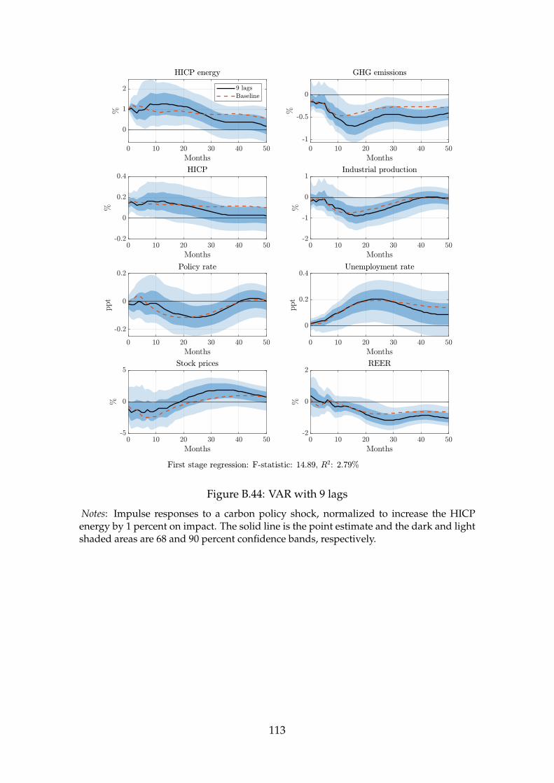
Figure B.44: VAR with 9 lags

Notes: Impulse responses to a carbon policy shock, normalized to increase the HICPenergy by 1 percent on impact. The solid line is the point estimate and the dark and lightshaded areas are 68 and 90 percent confidence bands, respectively.

113

Figure B.45: Bayesian VAR with shrinkage priors

Notes: Impulse responses to a carbon policy shock, normalized to increase the HICPenergy by 1 percent on impact. The solid line is the posterior median and the dark andlight shaded areas are 68 and 90 percent HPD bands, respectively.

114

C. Heteroskedasticity-based identification

As discussed in Section 8, we can also identify the structural impact vector underweaker assumptions, allowing for the presence of other shocks contaminating theinstrument over the daily event window. Suppose that movements in the EUAfutures zt we observe in the data are governed by both carbon policy and othershocks:

zt = ε1,t + ∑j 6=1

ε j,t + vt,

where ε j,t are other shocks affecting carbon futures and vt ∼ iidN(0, σ2v ) captures

measurement error such as microstructure noise. Because zt is also affected byother shocks, it is no longer a valid external instrument. However, we can stillidentify the structural impact vector by exploiting the heteroskedasticity in thedata.

The identifying assumption is that the variance of carbon policy shocks in-creases at the time of regulatory update events while the variance of all othershocks is unchanged. Define R1 as a sample of regulatory events in the EU ETSand R2 as a sample of trading days that do not contain an regulatory event butare comparable on other dimensions. R1 can be thought of as the treatment andR2 as the control sample (see Appendix B.5 for more information and some de-scriptive statistics of the instrument in the treatment and the control sample). Theidentifying assumptions can then be written as follows

σ2ε1,R1 > σ2

ε1,R2

σ2ε j,R1 = σ2

ε j,R2, for j = 2, . . . , n. (3)

σ2v,R1 = σ2

v,R2.

Under these assumptions, the structural impact vector is given by

s1 =ER1[ztut]−ER2[ztut]

ER1[z2t ]−ER2[z2

t ]. (4)

As shown by Rigobon and Sack (2004), we can also obtain this estimator throughan IV approach, using z = (z′R1, −z′R2)

′ as an instrument in a regression of thereduced-form innovations on z = (z′R1, z′R2)

′.

115

D. A heterogeneous-agent climate-economy model:

Derivations

In this appendix, I derive the theoretical model. As discussed in the main text, theaim is to obtain a framework that can account for the empirical findings – both atthe aggregate level and along the cross section – and can be used for policy exper-iments. The model combines a climate-economy structure in the spirit of Golosovet al. (2014) with nominal rigidities, household heterogeneity and risk. The modelconsists of four building blocks: households, firms, a government and a climateblock. The household block consists of two types of households: Households inthe hand-to-mouth (H) and savers (S) state, that differ in their MPCs, income in-cidence and energy shares. We incorporate idiosyncratic risk by assuming thathouseholds switch exogenously between types. The firm block is further dividedinto consumption good and energy producers. In this appendix, we go over eachmodel block in detail.

D.1. Labor market structure

To simplify matters, we assume a centralized labor market structure that equal-izes labor income across households; thus all income heterogeneity in the modelwill come from heterogeneity in financial income. This is a reduced-form way ofcapturing the income responses observed in the data.

We assume that there is a continuum of differentiated labor inputs indexed byj ∈ [0, 1].

Labor packer. There is a labor packer that bundles differentiated labor inputsinto aggregate labor demand according to a CES technology:

maxht(j)

wthd,t −∫ 1

0wt(j)ht(j)dj s.t. hd,t =

(∫ 1

0ht(j)

εw−1εw dj

) εwεw−1

The labor demand is

ht(j) =(

wt(j)wt

)−εw

hd,t.

and the aggregate wage wt is

wt =

(∫ 1

0wt(j)1−εw dj

) 11−εw

.

116

Unions. As in Schmitt-Grohé and Uribe (2005), each household supplies eachpossible type of labor. Wage-setting decisions are made by labor-type specificunions j ∈ [0, 1].5 Given the wage wt(j) fixed by union j, households stand readyto supply as many hours to the labor market j, ht(j), as demanded by firms

ht(j) =(

wt(j)wt

)−εw

hd,t,

where εw > 1 is the elasticity of substitution between labor inputs. Here, wt isan index of the real wages prevailing in the economy at time t and hd,t is theaggregate labor demand.

Households are distributed uniformly across unions and hence aggregate de-mand for labor type j is spread uniformly across households. It follows that theindividual quantity of hours worked, ht(i), is common across households andwe denote it as ht. This must satisfy the time resource constraint ht =

∫ 10 ht(j)dj.

Plugging in for the labor demand from above, we get

ht = hd,t

∫ 1

0

(wt(j)

wt

)−εw

dj.

The labor market structure rules out differences in labor income between house-holds without the need to resort to contingent markets for hours. The commonlabor income is given by

wthd,t =∫ 1

0wt(j)ht(j)dj = hd,t

∫ 1

0wt(j)

(wt(j)

wt

)−εw

dj.

Wage setting. Unions set their charged wages wj by maximizing a social welfarefunction, given by the weighted average of hand-to-mouth and savers’ utility,with the weights being equal to the shares of the households.6 The union problemreads

5This is different from the standard way of introducing sticky wages (see Erceg, Henderson,and Levin, 2000), which assumes that each household supplies a differentiated type of labor input.This assumption introduces equilibrium heterogeneity across households in the number of hoursworked. To avoid this heterogeneity from spilling over into consumption heterogeneity, it istypically assumed that preferences are separable in consumption and labor and that financialmarkets exists that allow agents to fully insure against unemployment risk. With the Schmitt-Grohé and Uribe (2005) formulation, one does not have to make these restrictive assumptions.

6This welfare function follows from the assumption that each household i supplies each pos-sible type of labor input j and there are a share of λ hand-to-mouth and a share of 1− λ savers.

117

maxwt(j)

(λ(xH,t)

1−σ − 11− σ

+ (1− λ)(xS,t)

1−σ − 11− σ

)− ϕ

h1+θt

1 + θ

s.t. ht = hd,t

∫ 1

0

(wt(j)

wt

)−εw

dj.

pS,txS,t + iS,t + bS,t+1 = hd,t

∫ 1

0wt(j)

(wt(j)

wt

)−εw

dj +Rb

t−1

ΠtbS,t + (1− τk)rtkS,t +

(1− τd)dt

1− λ+ ωS,t

pH,txH,t = hd,t

∫ 1

0wt(j)

(wt(j)

wt

)−εw

dj + ωH,t

The FOC is given by

λx−σH,t

1pH,t

hd,twεwt (1− εw)wt(j)−εw + (1− λ)x−σ

S,t1

pS,thd,tw

εwt (1− εw)wt(j)−εw =

ϕhθt hd,tw

εwt (−εw)wt(j)−εw−1

This rewrites

wt(j) =εw

εw − 1ϕhθ

t

(λ

1pH,t

x−σH,t + (1− λ)

1pS,t

x−σS,t

)−1

,

where εwεw−1 =Mw is the constant wage markup. By putting an optimal subsidy

in place, we can neutralize the markup and arrive at

wt(j) = ϕhθt

(λ

1pH,t

x−σH,t + (1− λ)

1pS,t

x−σS,t

)−1

.

Note that because everything on the right-hand-side is independent of j, itfollows that all unions charge the same wage wt(j) = wt. From the definition ofaggregate labor supply, we further have hd,t = ht.

Thus, wage setting is characterized by the following equation:

wt = ϕhθt

(λ

1pH,t

x−σH,t + (1− λ)

1pS,t

x−σS,t

)−1

.

D.2. Households

The household sector consists of a continuum of infinitely lived households, in-dexed by i ∈ [0, 1]. Households are assumed to have identical preferences withfelicity function U(x, h), deriving utility from consumption x and disutility fromlabor h. Households have access to three assets: a risk-free bond, shares in imper-fectly competitive firms, and physical capital.

118

Households participate infrequently in financial markets. When they do, theycan freely adjust their portfolio and receive dividends from firms and capital in-come. We call this the savers’ state (S). When agents do not participate in finan-cial markets, they can use only bonds to smooth consumption. We call this thehand-to-mouth state (H). We denote by s the probability to keep participatingin stock and capital markets in period t + 1, conditional upon participating at t,i.e. s = p(sj

t+1 = S|sjt = S), where sj

t is the current state of household j. Sim-ilarly, we call h the probability to keep being excluded from financial markets,i.e. h = p(sj

t+1 = H|sjt = H). Hence, the probability to become a financial mar-

ket participant is (1− h). The share of hand-to-mouth households thus evolvesas λt+1 = hλt + (1 − s)(1 − λt). We focus on the stationary equilibrium withλ = (1− s)/(2− s− h), which is the unconditional probability of being hand-to-mouth.

The requirement s ≥ 1− h ensures stationary and has a straightforward in-terpretation: the probability to remain in state S is larger than the probability tomove to state S (the conditional probability is larger than the unconditional one).In the limit case of s = 1− h = 1− λ, idiosyncratic shocks are iid: being S or Htomorrow is independent on whether one is S or H today. At the other extremestands TANK: idiosyncratic shocks are permanent (s = h = 1) and λ stays at itsinitial value (a free parameter).

We make two key assumptions to obtain a tractable representation. First, thereis perfect insurance among the households in a particular state but not betweenhouseholds in different states. Accordingly, we can think of households as liv-ing on two different islands and that within each island all resources are pooled.Households on the same island will thus make the same consumption and savingchoices. Second, however, we assume that stocks and capital are illiquid. Whensavers can no longer participate in financial markets, they cannot take their stockand capital holdings with them. Only bonds are liquid and can be transferredwhen switching between islands.

The timing is as follows. At the beginning of every period, resources withintypes are pooled. The aggregate shocks are revealed and households make theirconsumption and saving choices. Next, households learn their state in the nextperiod and have to move to the corresponding island accordingly, taking an(equally-split) fraction of the bonds on the current island with them.

The flows across islands are as follows. The total measure of households leav-ing the H island each period is the number of households who participate nextperiod: λ(1− h). The measure of households staying on the island is thus λh. Inaddition, a measure (1− λ)(1− s) leaves the S island for the H island at the end

119

of each period. Recall that our assumptions regarding insurance imply symmet-ric consumption/saving choices for all households in a given island. Denote bybS,t+1 the per-capita beginning-of-period t + 1 bonds of S (after the consumption-saving choice, and also after changing state and pooling). The end-of-period t percapita real values (after the consumption/saving choice but before agents moveacross islands) are zS,t+1. Likewise, bH,t+1 is the per capita beginning-of-periodt + 1 bonds in the H island (where the only asset is bonds). The end-of-periodt values (before agents move across islands) are zH,t+1. We have the followingrelations:

bS,t+1 = (1− λ)bS,t+1 = (1− λ)szS,t+1 + λ(1− h)zH,t+1

bH,t+1 = λbH,t+1 = (1− λ)(1− s)zS,t+1 + λhzH,t+1,

where bi,t+1, i ∈ S, H denote the bond holdings of the entire island. As stocksand capital do not leave the S island, we do not have to keep track of them.

Capital accumulation is simply characterized by:

kt+1 = it + (1− δ)kt

where δ is the depreciation rate.The program of savers reads

VS(bS,t, ωt, kt) = maxxS,t,zS,t+1,ωt+1,it,kt+1

(xS,t)1−σ

1− σ− ψ

h1+θt

1 + θ+ βEtVS(bS,t+1, ωt+1, kt+1)

+ βλ

1− λEtVH(bH,t+1)

subject to

pS,txS,t + zS,t+1 + νtωt+1

1− λ+

it

1− λ= wtht +

Rbt−1

Πt

bS,t

1− λ+(

νt + (1− τd)dt

) ωt

1− λ+ (1− τk)rt

kt

1− λ+ ωS,t

kt+1 = it + (1− δ)kt

bS,t+1 = (1− λ)szS,t+1 + λ(1− h)zH,t+1

bH,t+1 = (1− λ)(1− s)zS,t+1 + λhzH,t+1

zS,t+1 ≥ 0.

The household internalizes how aggregate bond holdings evolve according tohouseholds switching between types. Furthermore, the bond holdings a house-hold takes from an island cannot be negative, i.e. borrowing is not possible.

120

The first-order conditions read

x−σS,t

pS,t= λS,t

λS,t = β(1− λ)sEt[VSb (bS,t+1, ωt+1, kt+1)] + βλ(1− s)Et[VH

b (bH,t+1)] + ξS,t

λS,tνt

1− λ= βEt[VS

ω(bS,t+1, ωt+1, kt+1)]

λS,t

1− λ= βEt[VS

k (bS,t+1, ωt+1, kt+1)]

together with the complementary slackness condition:

zS,t+1ξS,t = 0,

with ξS,t ≥ 0. λS,t and ξS,t are Lagrange multipliers associated with the budgetand the inequality constraint, respectively.

From the Envelope theorem, we have

VSb (bS,t, ωt, kt) =

λS,t

1− λ

Rbt−1

Πt

VSω(bS,t, ωt, kt) =

λS,t

1− λ

(νt + (1− τd)dt

)VS

k (bS,t, ωt, kt) =λS,t

1− λ(1− (1− τk)rt − δ).

Using this in the FOCs gives

x−σS,t

pS,t= λS,t

λS,t = βsEt

[λS,t+1

Rbt

Πt+1

]+ βλ(1− s)Et[VH

b (bH,t+1)] + ξS,t

λS,t = βEt

[λS,t+1

νt+1 + (1− τd)dt+1

νt

]λS,t = βEt[λS,t+1(1− (1− τk)rt+1 − δ)].

The only thing that remains to be determined is VHb (bH,t+1). We can obtain

this from the problem of the hand-to-mouth.Their program reads

VH(bH,t) = maxxH,t,zH,t+1

x1−σH,t

1− σ− ψ

h1+θt

1 + θ+ βEtVH(bH,t+1) + β

1− λ

λEtVS(bS,t+1, ωt+1, kt+1)

121

subject to

pS,txH,t + zH,t+1 = wtht +Rb

t−1Πt

bH,t

λ+ ωH,t

bS,t+1 = (1− λ)szS,t+1 + λ(1− h)zH,t+1

bH,t+1 = (1− λ)(1− s)zS,t+1 + λhzH,t+1

zH,t+1 ≥ 0.

The first-order conditions read

x−σH,t = λH,t

λH,t = βλhEt[VHb (bH,t+1)] + β(1− λ)(1− h)Et[VS

b (bS,t+1, ωt+1, kt+1)] + ξH,t

together with the complementary slackness condition:

zH,t+1ξH,t = 0,

with ξH,t ≥ 0.From the Envelope theorem, we have

VHb (bH,t) =

λH,t

λ

Rbt−1

Πt.

Thus, we can rewrite the Euler equations for bonds accordingly

λH,t = βEt

[Rb

tΠt+1

(hλH,t+1 + (1− h)λS,t+1)

]+ ξH,t

and similarly for the savers:

λS,t = βEt

[Rb

tΠt+1

(sλS,t+1 + (1− s)λH,t+1)

]+ ξS,t.

Note that the Euler equation for stocks and capital are isomorphic to the con-ditions in a representative-agent setting. There is no self-insurance motive, forthey cannot be carried to the H state.7

In contrast, the bond Euler equations are of the same form as in fully-fledged

7As households pool resources when participating (which would be optimal with t=0 sym-metric agents and t = 0 trading), they perceive a return conditional on participating next period.This exactly compensates for the probability of not participating next period, thus generating thesame Euler equation as with a representative agent.

122

incomplete-markets models of the Bewely-Huggett-Aiyagari type. In particular,the probability (1− s) measures the uninsurable risk to switch to a bad state nextperiod, risk for which only bonds can be used to self-insure, thus generating ademand for bonds for “precautionary” purposes.

Two additional assumptions are required to deliver our simple equilibriumrepresentation. First, we focus on equilibria where (whatever the reason) theconstraint of H agents always binds (i.e. ξH > 0) and their Euler equation isin fact a strict inequality (for instance, because the shock is a “liquidity” or impa-tience shock making them want to consume more today, or because their averageincome in that state is lower enough than in the S state, as would be the caseif average profits were high enough; or simply because of a technological con-straint preventing them from accessing any asset markets) and the constraint ofS never binds (ξS = 0) so that their Euler equation always holds with equality.Second, we focus on the zero-liquidity limit, that is we assume that even thoughthe demand for bonds from S is well-defined (the constraint is not binding), thenet supply of bonds is zero, so there are no bonds traded in equilibrium.

Under these assumptions, the H households are indeed hand-to-mouth astheir budget constraint reads

pS,txH,t = wtht + ωH,t.

The intertemporal consumption/saving behavior by savers is characterizedby

λS,t =x−σ

S,t

pS,t

λS,t = βEt

[Rb

tΠt+1

(sλS,t+1 + (1− s)λH,t+1)

]

λS,t = βEt

[λS,t+1

νt+1 + (1− τd)dt+1

νt

]λS,t = βEt[λS,t+1(1− (1− τk)rt+1 − δ)]

pS,txS,t + iS,t + bS,t+1 = wtht +Rb

t−1Πt

bS,t + (1− τk)rtkS,t +(1− τd)dt

1− λ+ ωS,t

kt+1 = it + (1− δ)kt,

as market clearing implies that ωt = ωt+1 = 1.As to the intratemporal choice between energy and non-energy consumption,

recall that the final consumption bundle xS,t is a CES aggregate of consumption

123

and energy goods

xS,t =

(a

1εxS,cc

εx−1εx

S,t + a1

εxS,ee

εx−1εx

S,t

) εxεx−1

,

where aS,c and aS,e are distribution parameters with aS,c + aS,e = 18 , and εx is theelasticity of substitution between non-energy and energy goods: ∂(ct/ec,t)/(ct/ec,t)

∂(pe,t/1)/(pe,t/1) .9

Making the distribution parameters household-specific allows for heterogeneityin the households’ energy share.

The demands for the consumption and energy good the are given by

cS,t = aS,c

(1

pS,t

)−εx

xS,t

eS,t = aS,e

(pe,t

pS,t

)−εx

xS,t,

respectively. Note that the consumption good is chosen to be the numeraire, i.e.it’s price is one in real terms.

The corresponding price index is

pS,t =(

aS,c + aS,e p1−εxe,t

) 11−εx .

Similarly, for the hand-to-mouth, we have

cH,t = aH,c

(1

pS,t

)−εx

xH,t

eH,t = aH,e

(pe,t

pS,t

)−εx

xH,t

8Note that the distribution parameters aS,c and aS,e, sometimes also referred to as shares, arein fact not shares but depend on underlying dimensions unless εx = 1. In other words, theseparameters are not deep parameters but depend on a mixture of parameters that depends on thechoice of units. To circumvent this issue, we follow the re-parameterization approach proposedby Cantore and Levine (2012). In particular, we calibrate the steady-state energy share and to backout the implied distribution parameters. We have:

aS,e =peeSpSxS

(pe

pS

)εx−1= ωS,e

(pe

pS

)εx−1,

where ωS,e is the energy expenditure share. From this, we then have aS,c = 1− aS,e. Note that thisshare is dimensionless. Thus, we can calibrate or estimate it. By using this strategy, we can alsoperform comparative statics, varying the elasticity εx.

9If εx approaches ∞, the goods are perfect substitutes; if εx approaches 0, the goods are perfectcomplements; and if εx approaches 1, the goods are one-for-one substitutable, which correspondsto the Cobb-Douglas case.

124

and the price of their bundle is

pH,t =(

aH,c + aH,e p1−εxe,t

) 11−εx .10

D.3. Firms

The firm block of the model consists of two sectors: energy and non-energy pro-ducers. Importantly, non-energy firms also use energy as an intermediate inputto produce the non-energy good. Further, we assume that non-energy firms facesome restrictions in adjusting their prices while the energy sector does not faceany price rigidity.

Energy producers. The energy firm produces energy using labor only accordingto the following production function:

et = ae,the,t.

We assume that there is only a single source of energy (e.g. coal) that is availablein (approx.) infinite supply. Note that we measure energy in terms of carboncontent (carbon amount emitted). Energy firms are subject to a carbon tax. Forconvenience we model it as a sales tax τt, however, we can equally model it as aunit tax (see also the discussion in Golosov et al., 2014).

Their maximization problem reads

maxhe,t

(1− τt)pe,tet − wthe,t

s.t. et = ae,the,t

The FOC gives the optimal energy supply:

(1− τt)pe,tae,t = wt

(1− τt)pe,tet = wthe,twt

(1− τt)pe,t=

et

he,t.

Non-energy firms. To simplify matters, we split the non-energy goods sectorsinto two subsectors: a representative competitive final goods firm which aggre-

10Finally, their distribution parameters are given by aH,e = ωH,e

(pepH

)εx−1and vaH,c = 1− aH,e.

125

gates intermediate goods according to a CES technology and a continuum of in-termediate goods producers that produce different varieties using capital, energyand labor as an input. To the extent to which the intermediate goods are imperfectsubstitutes, there is a downward-sloping demand for each intermediate variety,giving the intermediate producers some pricing power. Importantly, however, in-termediate goods producers cannot freely adjust prices. Nominal price rigiditiesare modeled according to Calvo (1983) mechanism. In each period, a firm faces aconstant probability 1− θp of being able to reoptimize the nominal wage.

Final goods producer. Final goods firms maximize profits subject to the produc-tion function by taking prices as given. Since final goods firms are all identical,we can focus on one representative firm. These firms bundle the differentiatedgoods into a final good using a CES technology. Taking prices as given, the finalgoods producer chooses intermediate good quantities yt(i) to maximize profits:

maxyt(i)

Ptyd,t −∫ 1

0Pt(i)yt(i)di s.t. yd,t =

(∫ 1

0yt(i)

εp−1εp di

) εpεp−1

,

where yd,t is aggregate demand and εp > 1 is the elasticity of substitution. Whengoods are perfectly substitutable ε → ∞, we approach the perfect competitionbenchmark.

From the first order condition, we get the usual demand schedule

yt(i) =(

Pt(i)Pt

)−εp

yd,t.

From the zero profit condition we obtain the aggregate price level Pt =(∫ 10 Pt(i)1−εp dj

) 11−εp .

Intermediate goods producers. Intermediate inputs are produced by a con-tinuum of monopolistic firms indexed by i ∈ [0, 1] according to the followingconstant returns to scale technology, using capital kt(i), energy ey,t(i), and laborhy,t(i) as inputs

yt(i) = e−γst atkt(i)αey,t(i)νhy,t(i)1−α−ν, (5)

where at is TFP, and e−γst captures climate damages, modeled as a function of theatmospheric carbon concentration st.

As intermediate goods producers are monopolists, they maximize profits bytaking the demand function of final goods firms into account. We consider now

126

the problem of an intermediate goods firm i. For the sake of simplicity the pro-gram is split into two sub-problems: the cost minimization and the price settingproblem. To find the real cost function, factor costs are minimized subject to theproduction function. The program of firm i reads

minnt(i)

rtkt(i) + wthy,t(i) + pe,tey,t(i) s.t. yt(i) ≤ e−γst atkt(i)αey,t(i)νhy,t(i)1−α−ν

The FOCs read

rt = αλt(i)yt(i)kt(i)

pe,t = νλt(i)yt(i)ey,t(i)

wt = (1− α− ν)λt(i)yt(i)

hy,t(i)

where λt(i) is the corresponding Lagrange multiplier. This multiplier will againhave the interpretation as real marginal cost – how much will costs change if youare forced to produce an extra unit of output, i.e. mct(i) = λt(i). To prove this,let us solve for the Lagrange multiplier as a function of output. We have

λt(i) =1α

rtkt(i)yt(i)

=1ν

pe,tey,t(i)yt(i)

=1

1− α− νwt

hy,t(i)yt(i)

.

Thus,

kt(i) =α

1− α− ν

wt

rthy,t(i)

ey,t(i) =ν

1− α− ν

wt

pe,thy,t(i)

Plugging this in the constraint

yt(i) = e−γst at

(α

1− α− ν

wt

rt

)α ( ν

1− α− ν

wt

pe,t

)ν

hy,t(i).

From this we get the factor demand for labor, capital and energy

hy,t(i) = eγst

(α

1− α− ν

wt

rt

)−α ( ν

1− α− ν

wt

pe,t

)−ν yt(i)at

kt(i) = eγst

(α

1− α− ν

wt

rt

)1−α ( ν

1− α− ν

wt

pe,t

)−ν yt(i)at

ey,t(i) = eγst

(α

1− α− ν

wt

rt

)−α ( ν

1− α− ν

wt

pe,t

)1−ν yt(i)at

,

127

which in turn can be used to get the Lagrange multiplier

λt(i) = eγst α−αν−ν(1− α− ν)−(1−α−ν)rαt pν

e,tw1−α−νt

1at

.

Using the factor demands, we can solve for the cost function:

C(rt, pe,t, wt, yt(i)) = eγst α−αν−ν(1− α− ν)−(1−α−ν)rαt pν

e,tw1−α−νt

yt(i)at

Thus, one can see that the multiplier is equal to the marginal cost function:λt(i) = Cy(rt, pe,t, wt, yt(i)) = mct(i). Note that in the definition of the marginalcost (Lagrange multiplier) above, there is nothing that depends on i. Thus, itfollows that marginal costs are the same across firms, i.e mct(i) = mct.

Another important result can be obtained by dividing the two factor demands:

kt(i)hy,t(i)

=α

1− α− ν

wt

rt

kt(i)ey,t(i)

=α

ν

pe,t

rt

From this one can see that all firms hire capital and energy in the same ratio, i.e.kt(i)

hy,t(i)= kt

hy,tand ey,t(i)

hy,t(i)=

ey,thy,t

. This also implies that the output-capital, output-labor, and output-energy ratios are the same across firms.

Now that we have found the real cost function, we can move to the intermedi-ate goods firms’ price setting problem. Intermediate goods producers set pricesto maximize the expected discounted stream of (real) profits. However, as out-lined above, firms are not able to freely adjust price each period. In particular, ineach period there is a fixed probability of 1− θp that a firm can adjust its price.This means that the probability a firm will be stuck with a price one period is θp,for two periods is θ2

p, and so on (thus we assume independence from time sincelast price adjustment). Consider the pricing problem of a firm given the oppor-tunity to adjust its price in a given period. Since there is a chance that the firmwill get stuck with its price for multiple periods, the pricing problem becomesdynamic. Firms will discount profits s periods into the future by Mt,t+sθ

sp, where

Mt,t+s = βs λS,t+sλS,t

is the stochastic discount factor, which follows from the fact thatthe firm is owned by the savers. The price setting problem reads

maxPt(i)

Et

∞

∑k=0

(βθp)k λS,t+k

λS,t

(Pt(i)Pt+k

yt+k(i)−mct+kyt+k(i))

128

s.t.

yt+k(i) =

(Pt(i)Pt+k

)−εp

yd,t+k

∞

k=0

.

The FOC reads

Et

∞

∑k=0

(βθp)k λS,t+k

λS,t

((1− εp)Pt(i)−εp Pεp−1

t+k yd,t+k + εp mct+kPt(i)−εp−1Pεpt+kyd,t+k

)= 0.

Simplifying gives

Et

∞

∑k=0

(βθp)kλS,t+k

((1− εp)Pεp−1

t+k yd,t+k + εp mct+kPt(i)−1Pεpt+kyd,t+k

)= 0.

By rearranging, we obtain

Pt(i) =εp

εp − 1Et ∑∞

k=0(βθp)kλS,t+kmct+kPεpt+kyd,t+k

Et ∑∞k=0(βθp)kλS,t+kPεp−1

t+k yd,t+k

Note that nothing on the RHS depends on i. Thus, all firms will choose the samereset price P∗t = Pt(i).

We can write the optimal price more compactly as

P∗t =εp

εp − 1X1,t

X2,t

with

X1,t = Et

∞

∑k=0

(βθp)kλS,t+kmct+kPεp

t+kyd,t+k

X2,t = Et

∞

∑k=0

(βθp)kλS,t+kPεp−1

t+k yd,t+k.

We can also write the X’s recursively

X1,t = λS,tmctPεpt yd,t + βθpEtX1,t+1

X2,t = λS,tPεp−1t yd,t + βθpEtX2,t+1.11

11If θp = 0, then this would reduce to

P∗t =εp

εp − 1︸ ︷︷ ︸M

Pt mct,

129

Let us now rewrite these expressions in terms of inflation (as the price levelmay be non-stationary). Define x1,t =

X1,t

Pεpt

and x2,t =X2,t

Pεp−1t

. Thus, we have

x1,t = λS,tmctyd,t + βθpEtx1,t+1Πεpt+1

x2,t = λS,tyd,t + βθpEtx2,t+1Πεp−1t+1 .

The reset price equation then writes

P∗t =εp

εp − 1Pt

x1,t

x2,t

⇒ Π∗t =εp

εp − 1Πt

x1,t

x2,t,

where we define reset price inflation as Π∗t =P∗t

Pt−1.

Exploiting the Calvo assumption, we can write the aggregate price index as

Π1−εpt = (1− θp)(Π∗t )

1−εp + θp.

By way of summary, optimal behavior of firm i is characterized by

rt = αmctyt

kt

pe,t = νmctyt

ey,t

wt = (1− α− ν)mctyt

hy,t

Π∗t =εp

εp − 1Πt

x1,t

x2,t

x1,t = λS,tmctyd,t + βθpEtx1,t+1Πεpt+1

x2,t = λS,tyd,t + βθpEtx2,t+1Πεp−1t+1

Π1−εpt = (1− θp)(Π∗t )

1−εp + θp

yt(i) = e−γst atkt(i)αey,t(i)νhy,t(i)1−α−ν

The aggregate production is given by

yt =∫ 1

0yt(i)di =

∫ 1

0e−γst atkt(i)αey,t(i)νhy,t(i)1−α−νdi

i.e. the optimal price would be a fixed markup over nominal marginal cost. The distortion comingfrom this fixed markup over marginal cost can be easily eliminated using a constant subsidy. Inthis case we have thatM = 1 and

Pt = MCt

130

⇒ yt = e−γst atkαt eν

y,th1−α−νy,t = ∆tyd,t,

where we have exploited the fact that factors are hired in the same proportionand plugged in for the demand function. Note that there is a wedge betweenaggregate output and aggregate demand. The intuition is that with Calvo pric-ing, firms charging prices in different periods will generally have different prices,which implies that the model features price dispersion. When firms have differ-ent relative prices, there are distortions that create a wedge between betweenaggregate output measured in terms of production factor inputs and aggregatedemand measured in terms of the composite good. The higher the price disper-sion, the more labor and capital are needed to produce a given level of output.

We can also rewrite the dispersion term in terms of inflation making use of theCalvo assumption. We have

∆t = (1− θp)(Π∗t )−εp Π

εpt + θpΠ

εpt ∆t−1.

Firms profits are

dt =∫ 1

0

Pt(i)Pt

yt(i)di−mct

∫ 1

0yt(i)di.

Plugging in the demand function gives

dt = yd,tPεp−1t

∫ 1

0Pt(i)1−εp di−mctyd,t

∫ 1

0

(Pt(i)

Pt

)−εp

di.

Now since P1−εpt =

∫ 10 Pt(i)1−εp di, this reduces to

dt = yd,t −mctyd,t

∫ 1

0

(Pt(i)

Pt

)−εp

di

Thus, we can write profits as

dt = (1−mct∆t)yd,t.

Further, note that

mctyt = rtkt + pe,tey,t + wthy,t.

in the limiting case when prices are flexible. However, with sticky prices this markup will be timevarying, which introduces another distortion. In steady state, however, there will be no markup,i.e. real marginal costs will be one.

131

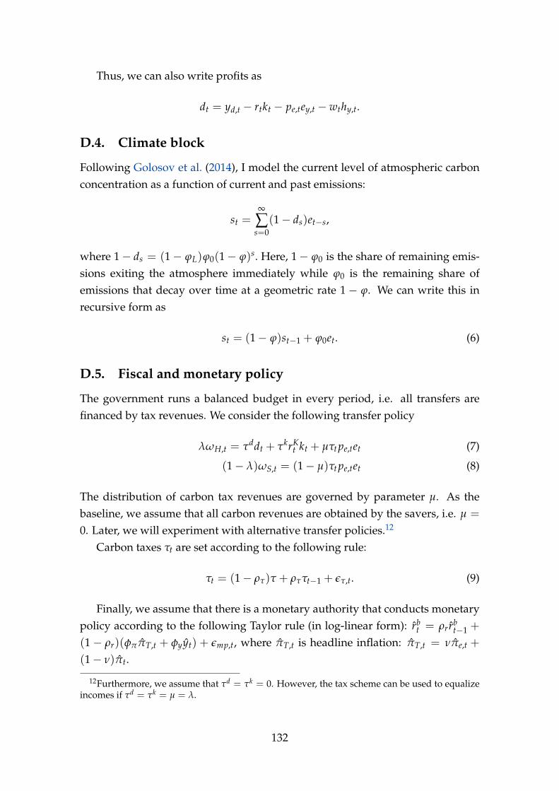
Thus, we can also write profits as

dt = yd,t − rtkt − pe,tey,t − wthy,t.

D.4. Climate block

Following Golosov et al. (2014), I model the current level of atmospheric carbonconcentration as a function of current and past emissions:

st =∞

∑s=0

(1− ds)et−s,

where 1− ds = (1− ϕL)ϕ0(1− ϕ)s. Here, 1− ϕ0 is the share of remaining emis-sions exiting the atmosphere immediately while ϕ0 is the remaining share ofemissions that decay over time at a geometric rate 1− ϕ. We can write this inrecursive form as

st = (1− ϕ)st−1 + ϕ0et. (6)

D.5. Fiscal and monetary policy

The government runs a balanced budget in every period, i.e. all transfers arefinanced by tax revenues. We consider the following transfer policy

λωH,t = τddt + τkrKt kt + µτt pe,tet (7)

(1− λ)ωS,t = (1− µ)τt pe,tet (8)

The distribution of carbon tax revenues are governed by parameter µ. As thebaseline, we assume that all carbon revenues are obtained by the savers, i.e. µ =

0. Later, we will experiment with alternative transfer policies.12

Carbon taxes τt are set according to the following rule:

τt = (1− ρτ)τ + ρττt−1 + ετ,t. (9)

Finally, we assume that there is a monetary authority that conducts monetarypolicy according to the following Taylor rule (in log-linear form): rb

t = ρr rbt−1 +

(1− ρr)(φππT,t + φyyt) + εmp,t, where πT,t is headline inflation: πT,t = νπe,t +

(1− ν)πt.

12Furthermore, we assume that τd = τk = 0. However, the tax scheme can be used to equalizeincomes if τd = τk = µ = λ.

132

D.6. Aggregation and market clearing

Because capital is only held by S, we have that (1−λ)kS,t = kt and (1−λ)iS,t = it.Because bonds are in zero net supply, we have zS,t = zH,t = bS,t = bH,t = 0.

Aggregate total, non-energy, and energy consumption are given by xt =

λxH,t + (1 − λ)xS,t, ct = λcH,t + (1 − λ)cS,t, and ec,t = λeH,t + (1 − λ)eS,t, re-spectively. Labor market clearing requires ht = hy,t + he,t. The energy marketclears if et = ec,t + ey,t.

Aggregate production is given by

yt =∫ 1

0yt(i)di = e−γst atkα

t eνy,th

1−α−νy,t = ∆tyd,t, (10)

where ∆t =∫ 1

0

(Pt(i)

Pt

)−εpdi is a price dispersion term, generating a wedge be-

tween aggregate output and aggregate demand.Finally, goods market clearing requires that

ct + it = yd,t. (11)

To derive this, we multiply the households budget constraints by their sharesand sum over them:

λpH,txH,t + (1− λ)(pS,txS,t + iS,t + bS,t+1) = λ(wtht + ωH,t) + (1− λ)

(wtht +

Rbt−1

ΠtbS,t + (1− τk)rtkS,t +

(1− τd)dt

1− λ+ ωS,t

)ct + it + pe,tec,t = wtht + rtkt + τt pe,tet + dt

ct + it + pe,tec,t = wtht + rtkt + τt pe,tet + yd,t − rtkt − wthy,t − pe,tey,t

ct + it = wthy,t + wthe,t + τt pe,tet + yd,t − wthy,t − pe,tet

ct + it = (1− τt)pe,tet + τt pe,tet + yd,t − pe,tet

ct + it = yd,t

D.7. Equilibrium

A general equilibrium of this economy is defined as a sequence of quantitiesQ = xt, xS,t, xH,t, ct, cS,t, cH,t, ec,t, eS,t, eH,t, it, kt+1, yt, yd,t, ht, hy,t, he,t, ey,t, mct, et, st, τt,ωH,t, dt, ∆t, x1,t, x2,t∞

t=0, a sequence of prices P =

λt, wt, rt, pe,t, pS,t, pH,t, Rbt , Πt, Π∗t , Πe,t, ΠT,t∞

t=0, and a sequence of forcingvariables F = at, ae,t, ετ,t, εmp,t∞

t=0 such that

1. Given a sequence of prices P , and a forcing sequence F , the sequence ofquantities Q solves the households’ and the firms’ problems.

133

2. Given a sequence of quantitiesQ and a sequence of forcing variables F , thesequence of prices P clears all markets.

The equilibrium is characterized by the following set of equations:

134

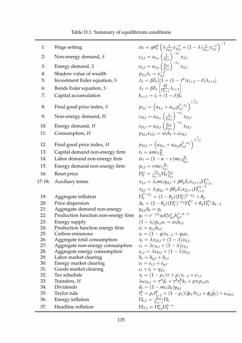
Table D.1: Summary of equilibrium conditions

1: Wage setting wt = ϕhθt

(λ 1

pH,tx−σ

H,t + (1− λ) 1pS,t

x−σS,t

)−1

2: Non-energy demand, S cS,t = aS,c

(1

pS,t

)−εxxS,t

3: Energy demand, S eS,t = aS,e

(pe,tpS,t

)−εxxS,t

4: Shadow value of wealth pS,tλt = x−σS,t

5: Investment Euler equation, S λt = βEt[(1 + (1− τk)rt+1 − δ)λt+1]

6: Bonds Euler equation, S λt = βEt

[Rb

tΠt+1

λt+1

]7: Capital accumulation kt+1 = it + (1− δ)kt

8: Final good price index, S pS,t =(

aS,c + aS,e p1−εxe,t

) 11−εx

9: Non-energy demand, H cH,t = aH,c

(1

pH,t

)−εxxH,t

10: Energy demand, H eH,t = aH,e

(pe,tpH,t

)−εxxH,t

11: Consumption, H pH,txH,t = wtht + ωH,t

12: Final good price index, H pH,t =(

aH,c + aH,e p1−εxe,t

) 11−εx

13: Capital demand non-energy firm rt = αmctytkt

14: Labor demand non-energy firm wt = (1− α− ν)mctyt

hy,t

15: Energy demand non-energy firm pe,t = νmctytey,t

16: Reset price Π∗t =εp

εp−1 Πtx1,tx2,t

17-18: Auxiliary terms x1,t = λtmctyd,t + βθpEtx1,t+1Πεpt+1

x2,t = λtyd,t + βθpEtx2,t+1Πεp−1t+1

19: Aggregate inflation Π1−εpt = (1− θp)(Π∗t )

1−εp + θp

20: Price dispersion ∆t = (1− θp)(Π∗t )−εp Π

εpt + θpΠ

εpt ∆t−1

21: Aggregate demand non-energy yd,t∆t = yt22: Production function non-energy firm yt = e−γst atkα

t eνy,th

1−α−νy,t

23: Energy supply (1− τt)pe,tet = wthe,t24: Production function energy firm et = ae,the,t25: Carbon emissions st = (1− ϕ)st−1 + ϕ0et26: Aggregate total consumption xt = λxH,t + (1− λ)xS,t27: Aggregate non-energy consumption ct = λcH,t + (1− λ)cS,t28. Aggregate energy consumption ec,t = λeH,t + (1− λ)eS,t29: Labor market clearing ht = hy,t + he,t30: Energy market clearing et = ec,t + ey,t31: Goods market clearing ct + it = yd,t32: Tax schedule τt = (1− ρτ)τ + ρττt−1 + ετ,t33: Transfers, H λωH,t = τddt + τkrK

t kt + µτt pe,tet34: Dividends dt = (1−mct∆t)yd,t35: Taylor rule rb

t = ρr rbt−1 + (1− ρr)(φππT,t + φyyt) + εmp,t

36: Energy inflation Πe,t =pe,t

pe,t−1Πt

37: Headline inflation ΠT,t = Πνe,tΠ

1−νt

135

D.8. Calibration and functional forms

The felicity function is assumed to be

U(xi,t, ht) =x1−σ

i,t − 1

1− σ− ψ

h1+θt

1 + θ,

for i ∈ H, S. This function belongs to the commonly used constant elasticityclass, where 1/σ is the intertemporal elasticity of substitution and 1/θ is the laborsupply elasticity.

We calibrate the model as follows. The time period is a quarter. The discountfactor β takes the standard value 0.99, which implies an annualized steady-stateinterest rate of 4 percent. The intertemporal elasticity of substitution 1/σ and thelabor supply elasticity 1/θ are set to 2. These values are at the upper range ofthe values commonly used in the literature, however, the results are qualitativelysimilar to using a more standard unitary elasticity. The labor weight in the utilityfunction, ϕ is calibrated such that steady-state hours worked h are normalizedto one. I set the share of hand-to-mouth λ to 25 percent, corresponding to thelow-income threshold used in the LCFS. Such a share is also in line with the es-timates of hand-to-mouth households in Kaplan, Weidner, and Violante (2014).Idiosyncratic risk is calibrated to 1− s = 0.04 as in Bilbiie (2020). The distributionparameters aH,e and aS,e are calibrated to match the energy expenditure shares of9.5 percent for the hand-to-mouth and 6.5 percent for the savers as observed inthe LCFS. The elasticity of substitution between energy and non-energy goods εx

is set to a moderate value of 0.75, implying that energy and non-energy goods areweak complements. This is motivated by the insignificant energy share responsein the data, however the results turn out to be robust to changing this elasticity.

Turning to the production side, I set the depreciation rate δ to 0.025, imply-ing an annual depreciation on capital of 10 percent. I set α to 0.275, which im-plies a standard steady-state capital share (rk/y) of 70 percent (see e.g. Smets andWouters, 2003). Using data on non-household energy consumption and energyprices in the EU, I estimate a energy share (peey/y) of around 7 percent. Thisis slightly higher than the energy share in the US, as estimated for instance byHassler, Krusell, and Olovsson (2012), and implies a value of ν = 0.085. The elas-ticity of substitution between non-energy varieties is assumed to be 6, which is astandard value and implies a steady-state markup of 20 percent, consistent withthe evidence in Christopoulou and Vermeulen (2012). The Calvo parameter θp isset to 0.825, which implies an average price duration of 5-6 quarters, in line withthe empirical estimates in Alvarez et al. (2006). These parameter choices imply a

136

relatively flat Phillips curve with a slope of 0.04.For the climate block, I rely on the values in Golosov et al. (2014). I abstract

from uncertainty about the damage parameter and use the deterministic, long-run value from Golosov et al. (2014). Note, however, that carbon emissions in mymodel are in arbitrary units. Thus, following Heutel (2012) I scale the damageparameter to make the increase in output damages from doubling the steady-state carbon stock consistent with the projected increase in damages from dou-bling CO2 levels in 2005. Turning to the carbon cycle, note that the excess car-bon has a half-life of about 300 years (Archer, 2005). This implies a value of1− ϕ = 0.9994.13 Furthermore, according to the 2007 IPCC reports, about halfof the CO2 pulse to the atmosphere is removed after a time scale of 30 years. Thisimplies that ϕ0 = 0.5

(1−ϕ)120 = 0.5359.Turning to fiscal and monetary policy, I compute the steady-state carbon tax

as the implied tax rate implied by the average EUA price which is around 3.9 per-cent (the average real EUA price as a share of gross electricity prices in emissionunits). The persistence of the tax shock is set to 0.9, which implies that the shockis close to being fully reabsorbed after about 20 quarters, which is consistent withthe shock dynamics observed in the external instruments VAR. Finally, the Tay-lor rule coefficient on inflation and output are set to 1.75 and 0.25, respectively,and interest smoothing is assumed to be 0.6. These values are standard in theliterature and compatible with the ECB’s mandate.

All other taxes are assumed to be zero in the baseline case, later we will usethem to equalize the income incidence. Furthermore, we assume that all carbontax revenues accrue to the savers, µ = 0, motivated by the fact that there is noredistribution scheme in the current EU ETS in place. The calibration is summa-rized in Table D.2.

13From the carbon cycle, we have Etst+h = (1− ϕ)hst = 0.5st. Thus, we impose (1− ϕ)1200 =0.5 to get ϕ.

137

Table D.2: Calibration

Parameter Description Value Target/Source

β Discount factor 0.99 Smets and Wouters (2003)1/σ Intertemporal elasticity of substi-

tution2 Standard macro-finance value/

Sensitivity1/θ Labor supply elasticity 2 Standard macro value/Sensitivity

ϕ Labor utility weight 0.783 Steady-state hours normalized to1

λ Share of hand-to-mouth 0.25 Share of low-income households,LCFS

1− s Probability of becoming H 0.04 Bilbiie (2020)aH,e Distribution parameter H 0.099 Energy share of 9.5%, LCFSaS,e Distribution parameter S 0.068 Energy share of 6.5%, LCFSεx Elasticity of substitution

energy/non-energy0.75 Weak complementarity

δ Depreciation rate 0.025 Smets and Wouters (2003)α Capital returns-to-scale 0.275 Steady-state capital share of 30%;

Smets and Wouters (2003)ν Energy returns-to-scale 0.085 Steady-state energy share of 7%;

Eurostatεp Price elasticity 6 Steady-state markup of 20%;

Christopoulou and Vermeulen(2012)

θp Calvo parameter 0.825 Average price duration of 5-6quarters; Alvarez et al. (2006)

γ Climate damage parameter 5.3 ∗ 10−5 Golosov et al. (2014)ϕ0 Emissions staying in atmosphere 0.5359 Golosov et al. (2014)

1− ϕ Emissions decay parameter 0.9994 Golosov et al. (2014)φπ Taylor rule coefficient inflation 1.75 Standard valueφy Taylor rule coefficient output 0.25 Standard valueρr Interest smoothing 0.6 Standard valueτ Steady-state carbon tax 0.039 Implied tax rate from average

EUA priceρτ Persistence carbon tax shock 0.9 Mean-reversion of approx. 20

quarters

D.9. Steady state and model solution

We assume that a = ae = 1 in steady state and we normalize ψ such that h = 1.Furthermore, τ is calibrated. Finally, we assume that there is zero inflation insteady state, i.e. Π = 1. From the definition of aggregate inflation and the pricedispersion, this implies Π∗ = 1, ∆ = 1 and yd = y.

From the investment Euler equation, we have

r =1β − 1 + δ

1− τk .

138

From the bonds Euler, we get

Rb =1β

.

From the reset price, we get

mc =εp − 1

εp.

To solve for the steady state, we guess k and e. From (13) with the aboveequation we get y.14 From (24), we get he. From (29), we get hy. From (25), we gets. From (22), we get ey. From (28), we get ec. From (15), we get pe. From (14), weget w. From (7), we get i. From (31), we get c. From (8), we get pS:

pS =(

aS,c + aS,e p1−εxe

) 11−εx

=(

1−ωS,e pεx−1e p1−εx

S + ωS,e p1−εxS

) 11−εx

= pS

(pεx−1

S −ωS,e pεx−1e + ωS,e

) 11−εx

⇒ 1 = pεx−1S −ωS,e pεx−1

e + ωS,e

pS =(

1 + ωS,e pεx−1e −ωS,e

) 1εx−1

.

From this we then have aS,e = ωS,e

(pepS

)εx−1and aS,c = 1− aS,e. Similarly we

get from (12) pH and aH,e and aH,c. From (34), we get d. From (33), we get ωH.From (11), we get xH. From (9), we get cH. From (10), we get eH. From (27), weget cS. From (28), we get eS. From (3), we get xS. From (26), we get x. From (4),we get λ. From (1), we get ψ. From (17)-(18), we get the values of the auxiliaryterms x1 and x2.Then we minimize such that (2) and (23) hold.

To solve the model, we log-linearize the equilibrium equations around thedeterministic steady state and solve for a set of linearized policy functions usingDynare.

14The equation numbers here refer to the equations in Table D.1.

139

References Appendix

Alloza, Mario, Pablo Burriel, and Javier J. Pérez. 2019. “Fiscal policies in the euro area:

Revisiting the size of spillovers.” Journal of Macroeconomics, 61: 103132.

Alvarez, Luis J., Emmanuel Dhyne, Marco Hoeberichts, Claudia Kwapil, Hervé Le Bi-han, Patrick Lünnemann, Fernando Martins, Roberto Sabbatini, Harald Stahl, andPhilip Vermeulen. 2006. “Sticky prices in the euro area: a summary of new micro-

evidence.” Journal of the European Economic Association, 4(2-3): 575–584.

Alves, Felipe, Greg Kaplan, Benjamin Moll, and Giovanni L. Violante. 2020. “A further

look at the propagation of monetary policy shocks in HANK.” Journal of Money, Creditand Banking, 52(S2): 521–559.

Archer, David. 2005. “Fate of fossil fuel CO2 in geologic time.” Journal of geophysical re-search: Oceans, 110(C9).

Baker, Scott R., Nicholas Bloom, and Steven J. Davis. 2016. “Measuring economic policy

uncertainty.” The Quarterly Journal of Economics, 131(4): 1593–1636.

Barnichon, Regis and Christian Brownlees. 2019. “Impulse response estimation by

smooth local projections.” Review of Economics and Statistics, 101(3): 522–530.

Baumeister, Christiane and James D. Hamilton. 2019. “Structural interpretation of vec-

tor autoregressions with incomplete identification: Revisiting the role of oil supply and

demand shocks.” American Economic Review, 109(5): 1873–1910.

Bilbiie, Florin O. 2020. “Monetary Policy and Heterogeneity: An Analytical Frame-

work.”

Bloom, Nicholas. 2009. “The impact of uncertainty shocks.” Econometrica, 77(3): 623–685.

Caldara, Dario, Michele Cavallo, and Matteo Iacoviello. 2019. “Oil price elasticities and

oil price fluctuations.” Journal of Monetary Economics, 103: 1–20.

Calvo, Guillermo A. 1983. “Staggered prices in a utility-maximizing framework.” Journalof Monetary Economics, 12(3): 383–398.

Cantore, Cristiano and Paul Levine. 2012. “Getting normalization right: Dealing with

‘dimensional constants’ in macroeconomics.” Journal of Economic Dynamics and Control,36(12): 1931–1949.

Christopoulou, Rebekka and Philip Vermeulen. 2012. “Markups in the Euro area and

the US over the period 1981–2004: a comparison of 50 sectors.” Empirical Economics,

42(1): 53–77.

Cloyne, James, Clodomiro Ferreira, and Paolo Surico. 2020. “Monetary policy when

households have debt: new evidence on the transmission mechanism.” The Review ofEconomic Studies, 87(1): 102–129.

Erceg, Christopher J., Dale W Henderson, and Andrew T. Levin. 2000. “Optimal mon-

etary policy with staggered wage and price contracts.” Journal of Monetary Economics,

46(2): 281–313.

Golosov, Mikhail, John Hassler, Per Krusell, and Aleh Tsyvinski. 2014. “Optimal taxes

140

on fossil fuel in general equilibrium.” Econometrica, 82(1): 41–88.

Hassler, John, Per Krusell, and Conny Olovsson. 2012. “Energy-saving technical

change.” National Bureau of Economic Research.

Heutel, Garth. 2012. “How should environmental policy respond to business cycles?

Optimal policy under persistent productivity shocks.” Review of Economic Dynamics,

15(2): 244–264.

Jarocinski, Marek and Peter Karadi. 2020. “Deconstructing monetary policy sur-

prises—the role of information shocks.” American Economic Journal: Macroeconomics,

12(2): 1–43.

Jordà, Òscar, Moritz Schularick, and Alan M. Taylor. 2015. “Betting the house.” Journalof International Economics, 96: S2–S18.

Kaplan, Greg, Justin Weidner, and Giovanni L. Violante. 2014. “The Wealthy Hand-to-

Mouth.” Brookings Papers on Economic Activity.

Kilian, Lutz. 2008. “Exogenous oil supply shocks: how big are they and how much do

they matter for the US economy?” The Review of Economics and Statistics, 90(2): 216–240.

Kilian, Lutz. 2009. “Not all oil price shocks are alike: disentangling demand and supply

shocks in the crude oil market.” American Economic Review, 99(3): 1053–69.

Känzig, Diego R. 2021. “The Macroeconomic Effects of Oil Supply News: Evidence from

OPEC Announcements.” American Economic Review, 111(4): 1092–1125.

Li, Dake, Mikkel Plagborg-Møller, and Christian K. Wolf. 2021. “Local Projections vs.

VARs: Lessons From Thousands of DGPs.”

Mansanet-Bataller, Maria and Angel Pardo. 2009. “Impacts of regulatory announce-

ments on CO2 prices.” The Journal of Energy Markets, 2(2): 1–33.

Montiel Olea, José Luis and Mikkel Plagborg-Møller. 2020. “Local Projection Inference

is Simpler and More Robust Than You Think.”

Plagborg-Møller, Mikkel and Christian K. Wolf. 2019. “Local projections and VARs es-

timate the same impulse responses.”

Plagborg-Møller, Mikkel and Christian K. Wolf. 2020. “Instrumental variable identifi-

cation of dynamic variance decompositions.”

Ramey, Valerie A. 2011. “Identifying government spending shocks: It’s all in the timing.”

The Quarterly Journal of Economics, 126(1): 1–50.

Ramey, Valerie A. and Sarah Zubairy. 2018. “Government spending multipliers in good

times and in bad: evidence from US historical data.” Journal of Political Economy,

126(2): 850–901.

Rigobon, Roberto. 2003. “Identification through heteroskedasticity.” Review of Economicsand Statistics, 85(4): 777–792.

Rigobon, Roberto and Brian Sack. 2004. “The impact of monetary policy on asset

prices.” Journal of Monetary Economics, 51(8): 1553–1575.

Schmitt-Grohé, Stephanie and Martin Uribe. 2005. “Optimal fiscal and monetary policy

in a medium-scale macroeconomic model.” NBER Macroeconomics Annual, 20: 383–425.

141

Smets, Frank and Raf Wouters. 2003. “An estimated dynamic stochastic general equilib-

rium model of the euro area.” Journal of the European Economic Association, 1(5): 1123–

1175.

142