THE U.S. ELECTORAL COLLEGE: ORIGINS AND TRANSFORMATION,

VARIANTS AND PROBLEMS

Nicholas R. MillerUMBC

LSE/VPP TalkMay 6, 2008

http://userpages.umbc.edu/~nmiller/ELECTCOL.html

Overview of Talk• Outline the original design of, and expectations

for, the Electoral College• Describe the rapid transformation of the

Electoral College into the popular vote-counting mechanism that exists today

• Identify criticisms of the Electoral College• Identify Variants of, and Alternatives to, the

Electoral College• Analyze the EC and variants with respect to (i)

voting power and (ii) election reversals. – The last is based on ongoing and incomplete

research.

Evaluations of the Electoral College• The mode of appointment of the Chief Magistrate of the

United States is almost the only part of the system, of any consequence, which has escaped without severe censure, or which has received the slightest mark of approbation from its opponents. . . . I venture somewhat further, and hesitate not to affirm that if the manner of it be not perfect, it is at least excellent. (Publius [Alexander Hamilton], Federalist 68):

• Many subsequent evaluations (and the many proposed constitutional amendments) suggest a less favorable assessment of “the mode of appointment of the Chief Magistrate,” which has been variously viewed as:– part of a generally elitist and anti-democratic constitution; or– a last-minute jerry-built compromise; or– a well designed compromise among diverse considerations, or possibly– the embodiment of well-thought selection criteria.

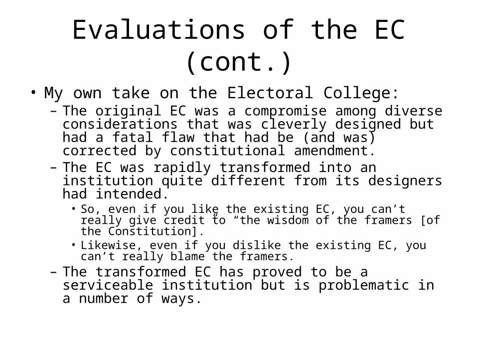
Evaluations of the EC (cont.)

• My own take on the Electoral College:– The original EC was a compromise among diverse

considerations that was cleverly designed but had a fatal flaw that had be (and was) corrected by constitutional amendment.

– The EC was rapidly transformed into an institution quite different from its designers had intended.

• So, even if you like the existing EC, you can’t really give credit to “the wisdom of the framers [of the Constitution].”

• Likewise, even if you dislike the existing EC, you can’t really blame the framers.

– The transformed EC has proved to be a serviceable institution but is problematic in a number of ways.

Origins of the Electoral College

• The original “Electoral College” [the term is not used in the Constitution] was a compromise between two modes of election of the President:– legislative election, which (it was feared) would make

the President subservient to Congress, and – national popular election, which presented formidable

practical difficulties at the time and reopened the conflict between large vs. small states.

• The perceived advantages of the Electoral College: – unlike Congress, the EC would perform a single task – i.e., cast

votes for President -- and would then disband; and– unlike popular election, the relative power of large vs. small

states could be compromised in the fine details of the EC (and public opinion could be refined).

The Original Electoral College Rules• Each state selects a number of “electors” equal in

number to its total (House + Senate) representation in Congress (H + 2).

• The legislature of each state determines the mode of selection of the electors from its state, the most likely alternatives being – election by the legislature itself,– popular election from districts, and– popular election on a state-wide “general ticket” [the almost universal

practice for the last 175 years].

• Electors were originally required to– cast two votes for two different candidates, – at least one of whom had to be a resident of another state.

• To be elected by the Electoral College, a candidate was required to receive – votes from a majority of electors and – more votes than any other candidate.– Given the double vote system, these requirements are logically distinct.

The Original Electoral College (cont.)

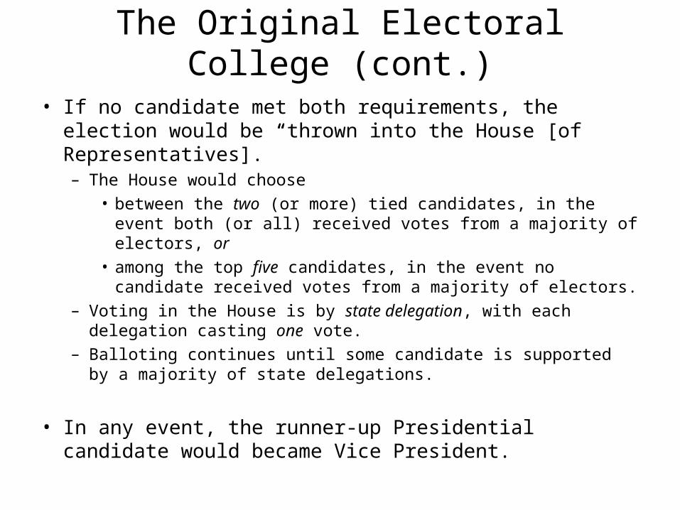
• If no candidate met both requirements, the election would be “thrown into the House [of Representatives].”– The House would choose

• between the two (or more) tied candidates, in the event both (or all) received votes from a majority of electors, or

• among the top five candidates, in the event no candidate received votes from a majority of electors.

– Voting in the House is by state delegation, with each delegation casting one vote.

– Balloting continues until some candidate is supported by a majority of state delegations.

• In any event, the runner-up Presidential candidate would became Vice President.

Expectations Concerning the Original EC• This original Electoral College system was designed to operate in a non-

partisan environment. – It therefore was expected that

• typically there would be many potential Presidential candidates, and• electors would choose among these candidates on the basis of their

character and connections, not party affiliation or policy promises.

– Therefore, it was also expected that the “House contingent procedure” would be needed “19 times out of 20,” so

• big states would have the dominant role in “screening/nominating” candidates (in the EC), while

• small states would have equal role in most final elections (in the House).

• It was generally hoped and expected that electors would typically be – popularly elected – from single-member districts (like most state legislators, delegates to

the state ratifying conventions, members of the House of Commons, and as was expected also for members of the new U.S. House); and

– that they would be well-informed local notables who would act as representative trustees of their states and districts.

Duverger’s Law and Crackup of the Original Electoral College

• These expectations did not anticipate the development of a national two-party system.

• Duverger’s Law: Given politically ambitious candidates, single-winner elections produce (in equilibrium) two-candidate contests [by virtue of the “wasted vote” argument, etc.] and sustain a two-party system.

• Given the development of a two-party [Federalist vs. Republican] system, the combination of the double-vote and runner-up-is-VP provisions of the original Electoral College turned out to be a fatal flaw. – In 1796 the Presidential candidate (Jefferson) of the losing

(Republican) party became Vice President.– In 1800 an electoral vote tie between the two (Presidential and

Vice Presidential) candidates of the winning (Republican) party was broken by a House of Representatives controlled by the losing (Federalist) party.

The 12th Amendment• After the 1800 fiasco, Congress proposed, and the

states quickly ratified (in time for 1804 election), the 12th Amendment to the Constitution. – Electors now cast separate (single) votes for President and Vice

President.– The required electoral vote majority for President (and for Vice

President) is a simple majority of votes cast (= number of electors), which at most one candidate can achieve.

– If no candidate receives the required simple majority for President, the House (still voting by state delegations) chooses from among the top three [vs. top five] candidates.

– If no candidate receives the required majority for Vice President, the Senate (voting individually) chooses from among the top two candidates.

• This remains the constitutional language governing Presidential elections.

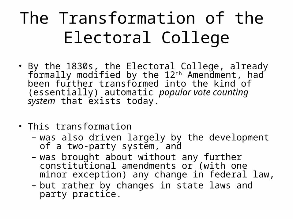
The Transformation of the Electoral College

• By the 1830s, the Electoral College, already formally modified by the 12th Amendment, had been further transformed into the kind of (essentially) automatic popular vote counting system that exists today.

• This transformation – was also driven largely by the development of a two-

party system, and– was brought about without any further constitutional

amendments or (with one minor exception) any change in federal law,

– but rather by changes in state laws and party practice.

Elements of the Transformation• The way the rival parties first contested a Presidential

election was to secure the selection of electors expected to cast electoral votes for their Presidential and Vice Presidential candidate.

• Beginning even with the first contested Presidential election in 1796, elector candidates were therefore almost invariably “party men,” pledged (and faithful) to the (Presidential and Vice Presidential) nominees of their party.– Put otherwise, electors became party delegates rather that trustees of

their states or districts [cf. regular delegates vs. superdelegates]– Pledged electors were almost universal as early as 1796.

• Notably, Samuel Miles (Fed., PA) violated his pledge and voted for Jefferson rather than Adams.

• An angry Federalist supporter complained: “What, do I choose Samuel Miles to determine for me whether John Adams or Thomas Jefferson shall be President? No! I choose him to act, not to think.”

– Once pledged and faithful electors have been selected, the prospective electoral vote for Presidential candidates is also known.

Elements of the Transformation (cont.)• In early elections, the mode of selecting Presidential electors was

regularly manipulated by party politicians in each state, on the basis of partisan calculations.– Madison to Monroe (1800): “All agree that an election by districts

would be best if it could be general, but while ten states choose either by their legislatures or by a general ticket [so the dominant party wins all of a state’s electoral votes], it is folly or worse for the other six not to follow.”

• By 1832, Presidential electors were almost universally selected by popular (vs. legislative) vote (and by much expanded electorates).

• By 1836, the mode of popular election in every state is (following Madison’s strategic advice above) the general ticket (or party slate), rather than election from districts (or by some kind of proportional representation).– This induced the almost universal “winner-take-all” rule for the

casting electoral votes at the state level.– However, at the present time two small states (ME and NE) use

the “Modified District Plan.”

Elements of the Transformation (cont.)• Moreover, the two-party system bypasses the House contingent

procedure at least “19 times out of 20.”– On this point, the election of 1824 (the second and last time an election

was thrown into the House) was the “exception that proved the rule”.• The Federalist Party had collapsed and the Democratic-Republican

Party was unchallenged.• Consequently there was no longer pressure for D-Rs to unite behind a

single Presidential-Vice Presidential ticket.• Four candidates, all nominally belonging to the same D-R party,

sought the Presidency.• Unsurprisingly, no candidate received a majority of the electoral votes

and the election was thrown into the House (for the second and last time).

– However, whenever there is a “serious” third-party ticket (especially one with a geographical base of support such that it may win electoral votes), the possibility than the election may be thrown into the House arises.

– Moreover, since the 23rd Amendment (giving the District of Columbia three electoral votes) was ratified in 1961, the total number of electoral votes has been an even number (538),

• so an electoral vote tie (269-269) is possible, and• an election might be thrown into the House even in the absence of a

third-party candidate winning election votes.

The EC as a Vote-Counting Mechanism• In 1845 Congress established a uniform nationwide Presidential election

day (i.e., day for selecting Presidential electors) • On November 4, 2008, voters in each state will go to the polls and vote for

either the Democratic or Republican (or possibly other) slate of elector candidates, who are pledged to their party’s (Pres. + VP) nominees. – With popular election of pledged electors, American voters may be

forgiven for thinking they are actually voting directly for Presidential candidates (often there is little on the ballot to suggest otherwise).

• In each state, the elector slate receiving the most votes wins.• The electors will meet in their state capitals in mid-December and cast their

electoral votes as pledged.• Electoral vote tallies will be transmitted from each state capital to Congress

and are counted before a joint session on January 5, 2009.• The President of the Senate [Vice President Cheney] will announces the

vote and proclaimed that ??? is the President-elect.• So in (almost invariable) practice, everything will be determined on election

night in November, and the remaining steps are merely ceremonial; that is, TV prognosticators can– report the popular vote winner in each state,– add up the corresponding electoral votes, and– declare a President-elect.

(Alleged) Problems with the EC as a Vote-Counting Mechanism

• The Voting Power Problem. Does the EC [or EU] give voters in different states [member nations] unequal voting power?– If so, the EC [EU] violates the criterion of “One Person, One Vote” (OPOV).– Which voters are favored and which disfavored and by how much?

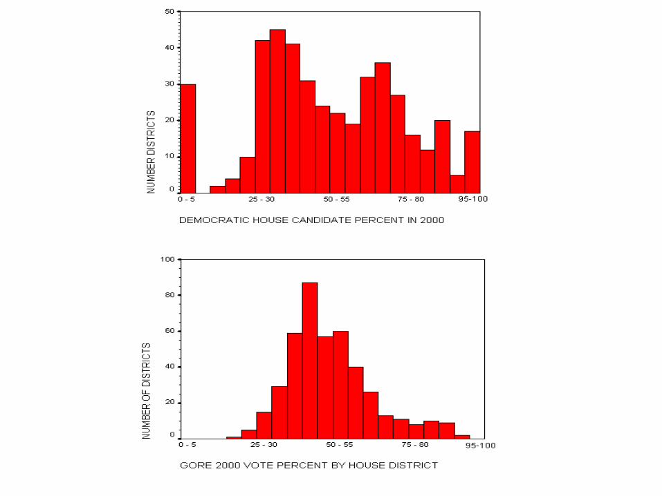
• The Election Reversal Problem. The candidate who wins the most popular votes nationwide may fail to be elected.– The election 2000 provides an example (provided we take the official

popular vote in FL at face value).• The Partisan Bias Problem. Does the EC as a vote counting system

favor one party over the other (at the present time or in times past)?– This is closely connected with the Election Reversal Problem.

• The Battleground States Problem. The Electoral College focuses the Presidential election contest on a few “battleground states,” which get very disproportionate attention from the candidates and parties.– This is loosely connected with the Voting Power Problem.

• Other Problems -- mere vote-counting may fail.– What if electors violate their pledges?– The House contingent procedure.– Americans have “no constitutional right to vote for President.”

EC Variants: The Apportionment of Electoral Votes

• Keep the winner-take all practice [in 2000, Bush 271, Gore 267; in 2004, Bush 286, Kerry, 252] but use a different formula to apportioning electoral votes among states (All require a constitutional amendment.)

– Apportion electoral votes [in whole numbers] on basis of House seats only] [Bush 211, Gore 225; Bush 224, Kerry 212]

• Apportion electoral votes [fractionally] precisely proportional to population [Bush 268.96092, Gore 269.03908; Bush 275.67188, Kerry 262.32812]

Translated outcomes take account of Duverger’s “mechanical effects” only (vs. “psychological/strategic effects”)

EC Variants: The Apportionment of Electoral Votes (cont.)

• Apportion electoral votes [fractionally] to be precisely proportional to population but then add back the “constant two” [Bush 277.968, Gore 260.032; Bush 285.407, Kerry 252.593]

• Apportion electoral votes equally among the states [in the manner of the House contingent procedure] [Bush 30, Gore 21; Bush 31, Kerry 20]

– National Bonus Plan: 538 electoral votes are apportioned and cast as at present but an additional bloc of electoral votes [e.g., 100] are awarded on a winner-take-all basis to the national popular vote winner. [Bush 271, Gore 367; Bush 386, Kerry 252]

EC Variants: The Casting of Electoral Votes

• Apportion electoral votes as at present but use something other than winner-take-all for casting state electoral votes. (Some can be adopted on a state-by-state basis.) All are likely to produce splits in state electoral votes.

– Pure District Plan: select electors from single-member districts (as originally expected), so each electoral vote is cast for the district winner.

– Modified District Plan: select the two “Senate electors” statewide and the “House electors” by district [probably CDs -- present NE and ME practice]. [Bush 289, Gore 249; I don’t have good data for 2004]

EC Variants: The Casting of Electoral Votes (cont.)

– Pure Proportional Plan: electoral votes are cast [fractionally] in precise proportion to state popular vote. [Bush 259.2868, Gore 258.3364, Nader 14.8100, Buchanan 2.4563, Other 3.1105; Bush 277.857, Kerry 260.143 (excluding minor candidates)] (implies doing away with electors as individuals)

– Whole Number Proportional Plan [e.g., Colorado Prop. 36]: electoral votes are cast in whole numbers on the basis of some (PR-style) apportionment formula applied to each state’s popular vote. [Bush 263, Gore 269, Nader 6, or Bush 269, Gore 269; Bush 280, Kerry 258]

The Popular Vote Alternative to the EC• Elect the President and Vice President on the basis the popular vote

of the nation as a whole.– Requires national election administration, voter qualifications and

registration, ballot access rules, etc.?– Runoff requirement? With what threshold?

• Supplementary vote [like London mayor], IRV etc.?

• To bypass the constitutional amendment process, adopt the National Popular Vote Plan,– to be effected by interstate compact (which requires the consent of

Congress but not a constitutional amendment).– The states in the compact pledge to cast their electoral votes for the

national popular vote winner.– Problems:

• There is no official “national popular vote winner.”• The Plan largely ignores general popular vote problems noted

above.• Would the compact hold in an election like 2000 (i.e., in which there

would be an election reversal if the EC operated in the normal manner)?

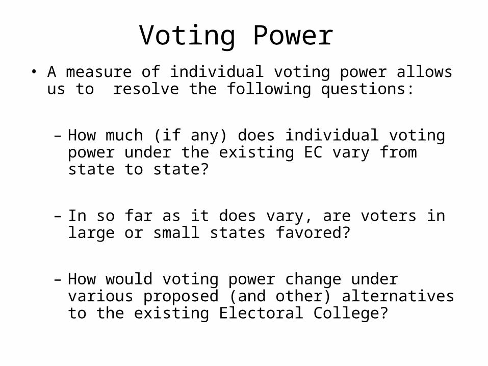
Voting Power • A measure of individual voting power allows us to

resolve the following questions:

– How much (if any) does individual voting power under the existing EC vary from state to state?

– In so far as it does vary, are voters in large or small states favored?

– How would voting power change under various proposed (and other) alternatives to the existing Electoral College?

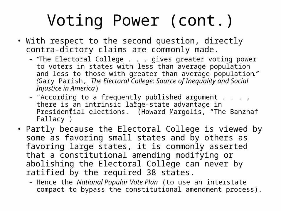
Voting Power (cont.)• With respect to the second question, directly contra-

dictory claims are commonly made.– “The Electoral College . . . gives greater voting power to voters

in states with less than average population and less to those with greater than average population.” (Gary Parish, The Electoral College: Source of Inequality and Social Injustice in America)

– “According to a frequently published argument . . . , there is an intrinsic large-state advantage in Presidential elections.” (Howard Margolis, “The Banzhaf Fallacy”)

• Partly because the Electoral College is viewed by some as favoring small states and by others as favoring large states, it is commonly asserted that a constitutional amending modifying or abolishing the Electoral College can never by ratified by the required 38 states.– Hence the National Popular Vote Plan (to use an interstate

compact to bypass the constitutional amendment process).

Voting Power (cont.)

• First, we need to define and distinguish between– voting weight and – voting power.

• With respect to the Electoral College, we need to bear in mind the distinctions already made between – how electoral votes are apportioned among the states

(which determines voting weight), and– how electoral votes are cast within states (which, in

conjunction with voting weight, determines voting power).

The Apportionment of Electoral Votes• The apportionment of electoral votes (voting weights)

produces a systematic and substantial small-state advantage in the apportionment of electoral votes relative to the apportionment population.– This is the basis of the argument that the Electoral College

advantages voters in smaller (rural, more conservative, etc.) states.

• The magnitude of this small-state apportionment advantage is not fixed in the Constitution.– It varies (inversely) with the size of the House (relative to the

Senate), which is determined by Congress.– If the House had been sufficiently larger than 435, Gore would

have won the 2000 election (even while losing Florida).

The Small-State Apportionment Advantage

Another View of the Small-State Advantage

The Casting of Electoral Votes

• Remember that state choice of the general ticket for electing electors produces the winner-take-all practice that produces the weighted voting game noted at the outset.

• Many have believed that this practice produces a large-state advantage in voting power that counteracts (in some degree) the small-state advantage in apportion-ment. – This is the basis for the argument that the Electoral College

gives disproportionate voting power to voters in larger (urban, ethnically diverse, etc.) states.

A Priori Voting Power• An appropriate voting power measure can evaluate the

voting power of each state in the Electoral College weighted voting game with 51 voters.

• In addition, there is a large-number unweighted majority voting game within each state that determines how that state will vote in the Electoral College.

• So the overall Presidential election is a two-tier voting game.– The measurement and interpretation of a priori voting power has been a

major focus of the LSE program on Voting Power and Procedures.– Though VPP research has focused primarily on voting power with

respect to the EU Council of Ministers (and other EU institutions).

• Measures of a priori voting power applied to the Electoral College (or the EU) take account only of the its formal rules plus the population of each state and the mathematical formula used to apportion House seats among the states,– but not demographics, historic voting patterns, ideology, polling results,

election forecasts, etc.

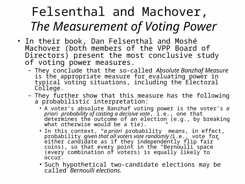
Felsenthal and Machover, The Measurement of Voting Power

• In their book, Dan Felsenthal and Moshé Machover (both members of the VPP Board of Directors) present the most conclusive study of voting power measures.– They conclude that the so-called Absolute Banzhaf Measure is

the appropriate measure for evaluating power in typical voting situations, including the Electoral College.

– They further show that this measure has the following a probabilistic interpretation:

• A voter’s absolute Banzhaf voting power is the voter’s a priori probability of casting a decisive vote, i.e., one that determines the outcome of an election (e.g., by breaking what otherwise would be a tie).

• In this context, “a priori probability” means, in effect, probability given that all voters vote randomly (i.e., vote for either candidate as if they independently flip fair coins), so that every point in the “Bernoulli space” (every combination of voters) is equally likely to occur.

• Such hypothetical two-candidate elections may be called Bernoulli elections.

Calculating Power Index Values

• There are mathematical formulas and algorithms can calculate or estimate voting power values.

• Various website make these algorithms readily available.• One of the best of these is the website created by

Dennis Leech (University of Warwick and another VPP Board member): Computer Algorithms for Voting Power Analysis,

http://www.warwick.ac.uk/~ecaae/

which was used in making most of the calculations that follow.

Share of Voting Power by Share of Electoral Votes

Share of Voting Power by Share of Population

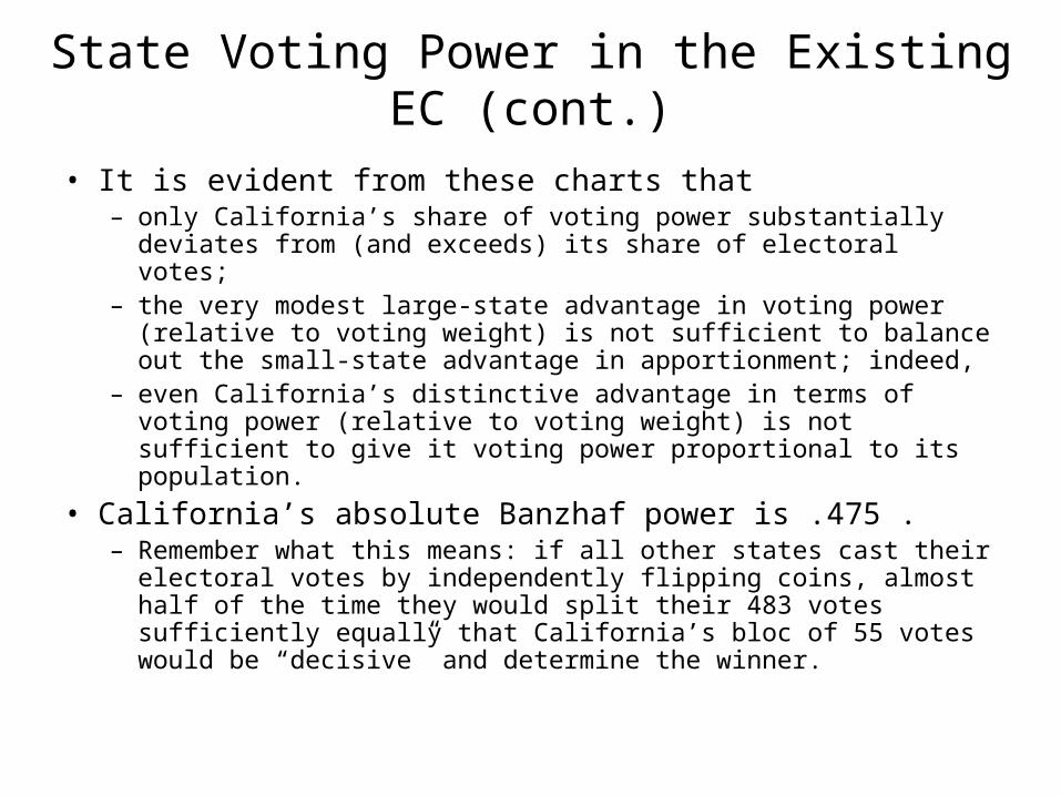
State Voting Power in the Existing EC (cont.)

• It is evident from these charts that– only California’s share of voting power substantially deviates

from (and exceeds) its share of electoral votes;– the very modest large-state advantage in voting power (relative

to voting weight) is not sufficient to balance out the small-state advantage in apportionment; indeed,

– even California’s distinctive advantage in terms of voting power (relative to voting weight) is not sufficient to give it voting power proportional to its population.

• California’s absolute Banzhaf power is .475 .– Remember what this means: if all other states cast their electoral

votes by independently flipping coins, almost half of the time they would split their 483 votes sufficiently equally that California’s bloc of 55 votes would be “decisive” and determine the winner.

The 125 Million Two-Tier Voting Game

• But as previously noted, a U.S. Presidential election really is a two-tier voting system, in which the casting of electoral votes is determined by a simple majority voting games within each state.

• In such a two-tier system, individual a priori voting power is the probability of “double decisiveness,” i.e., – that a voter casts a decisive vote within his or her state (i.e., that

there is tie among the other voters in the state), and

– that his or her state casts a decisive bloc of electoral votes (i.e., that neither candidate wins 270 electoral votes from the other states).

• Put otherwise, individual voting power in the two-tier system is equal to– individual voting power in the unweighted (but large number)

majority voting game within the state times

– the state’s voting power in the 51-state weighted voting game.

The Two-Tier Voting Game (cont.)

• Probability theory and the properties of Banzhaf measure tell us that the individual voting power in the first tier (within state) voting game is inversely proportional (to excellent approximation once n ~> 25) to the square root of the number of voters in the state.

• We previously saw that a state’s voting power in the second tier voting game is approximately proportional to its electoral vote (and therefore, apart from the small- state apportionment advantage, roughly proportional to its population).

• Putting these two considerations together, it follows that individual a priori voting power in the two-tier system – increases with the population of the voter’s state, and – is approximately proportional to the square root of the

number of voters in the voter’s state.

Individual Voting Power Under the Existing EC• The following chart shows how individual voting power under the

existing Electoral College varies by state population.• It also shows:

– mean individual voting power nationwide, and– individual voting power under direct popular vote (calculated in the same

manner as individual voting power within a state).• This is necessarily uniform over the nation.• Note that it is substantially greater than mean individual voting

power under the Electoral College.– Indeed, it is greater than individual voting power in every state

except California. – By the criterion of a priori voting power, only voters in California would

be hurt if the existing Electoral College were replaced by a direct popular vote.

Methodological note: in most of the following charts, individual voting power is scaled so that the voters in the least favored state have a value of 1.000, so

– numerical values are not comparable from chart to chart, and– the scaled value of individual voting power under direct popular vote

changes from chart to chart.

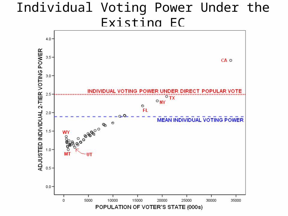
Individual Voting Power Under the Existing EC

“House Electoral Votes” Only

Electoral Votes Precisely Proportional to Population

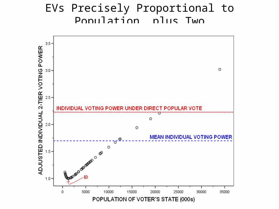
EVs Precisely Proportional to Population, plus Two

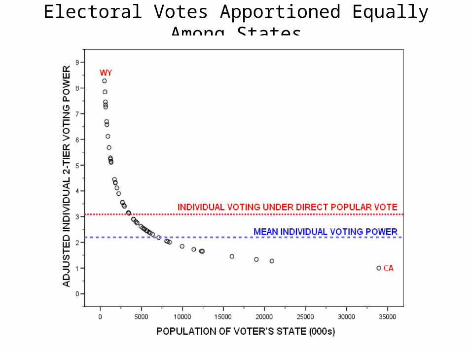
Electoral Votes Apportioned Equally Among States

Individual Voting Power under Alternative Rules for Casting Electoral Votes

• Calculations for the Pure District Plan, Pure Proportional Plan, and the Whole-Number Proportional Plan are straightforward.

• Under the Modified District Plan (or National Bonus Plan), each voter casts a single vote that counts two ways:

• within the district (or state) and • at-large (i.e., within the state or nation).

– Calculating individual voting power in such systems is far from straightforward.

– I am in the process of working out approximations based on very large samples of Bernoulli elections.

Pure District System

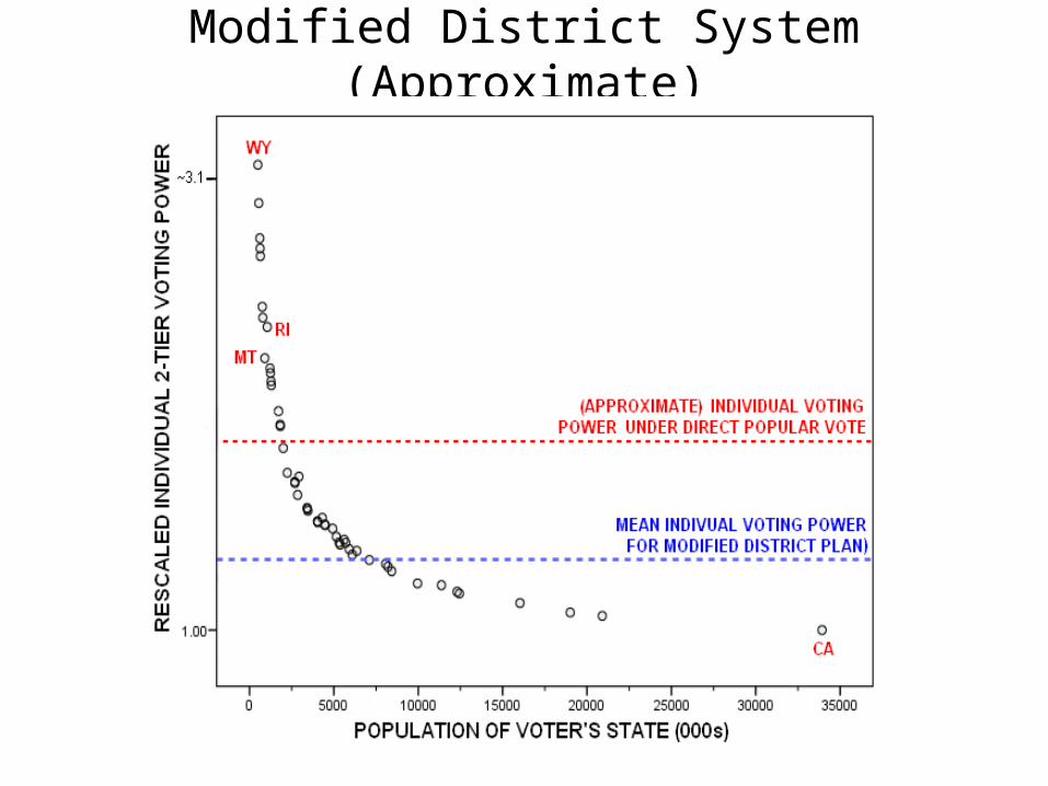
Modified District System (Approximate)

A Unilateral Move From Winner-Take-All to the (Pure) District System

• In the mid-1990s, the Florida state legislature seriously considered switching to the Modified District Plan.

• The effect of such a switch on the individual voting power is shown in the following chart.– However, I assume a switch to the Pure District Plan, because

it is much easier to calculate. – Madison’s earlier strategic advice is powerfully confirmed,

• though the voting-power consideration is logically distinct from the party-advantage consideration Madison had in mind,

• But the latter is also illustrated: considering “mechanical” effects only, if Florida had made the switch, Gore would have been elected President (regardless of the statewide vote in Florida).

• Even if a district system is universally agreed to be socially superior (as Madison considered it), states will not voluntary choose to move that direction. – States are faced with a “Prisoners’ Dilemma.”

(Pure) Pure Proportional System

The Whole-Number Proportional Plan• This plan divides a state’s electoral votes between (or among) the

candidates in a way that is as close to proportional to the candidates’ state popular vote shares as possible, given that the apportionment must be in whole numbers.– Unlike the (Pure) Proportional Plan, whole-number

proportionality allows for the retention of electors.– Accordingly, it is the only proportional plan that can be

implemented at the state level (as Colorado Prop. 36 proposed).– Colorado Proposition 36 used a distinctly ad hoc apportionment

formula. • But, in the event there are just two candidates (as in Bernoulli

elections), all apportionment formulas work in the same straightforward way:– multiply each candidate’s share of the popular vote by the state’s

number of electoral votes and then round off in the normal manner.

• The following chart shows that this plan produces a truly bizarre distribution of voting power.

Whole-Number Proportional Plan

Similar calculations and chart were produced, independently and earlier, by Claus Beisbart and Luc Bovens, “A Power Analysis of the Amend-ment 36 in Colorado,” University of Konstanz, May 2005, and Public Choice, March 2008.

National Bonus Plan(s)

Individual Voting Power: Summary Chart

Election Reversals• Any districted electoral system can produce an election

reversal. – That is, the candidate or party that wins the most

popular votes nationwide may fail to win the most parliamentary seats or electoral votes (and therefore lose the election).

– Such outcomes are actually more common in some parliamentary systems than in U.S. Presidential elections.

• The U.S. Electoral College has produced three manifest election reversals (though all were very close). outcomes)– But the mother of all EC election reversals is not

usually recognized as such.

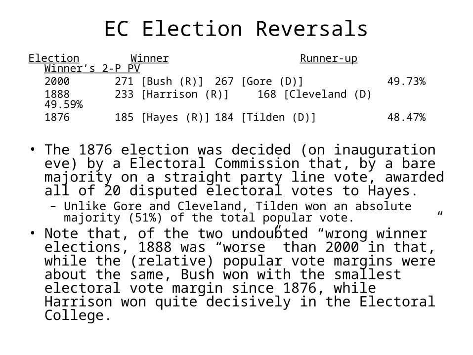
EC Election Reversals Election Winner Runner-up Winner’s 2-P PV

2000 271 [Bush (R)] 267 [Gore (D)] 49.73%1888 233 [Harrison (R)] 168 [Cleveland (D) 49.59% 1876 185 [Hayes (R)] 184 [Tilden (D)] 48.47%

• The 1876 election was decided (on inauguration eve) by

a Electoral Commission that, by a bare majority on a straight party line vote, awarded all of 20 disputed electoral votes to Hayes. – Unlike Gore and Cleveland, Tilden won an absolute majority

(51%) of the total popular vote.• Note that, of the two undoubted “wrong winner”

elections, 1888 was “worse” than 2000 in that, while the (relative) popular vote margins were about the same, Bush won with the smallest electoral vote margin since 1876, while Harrison won quite decisively in the Electoral College.

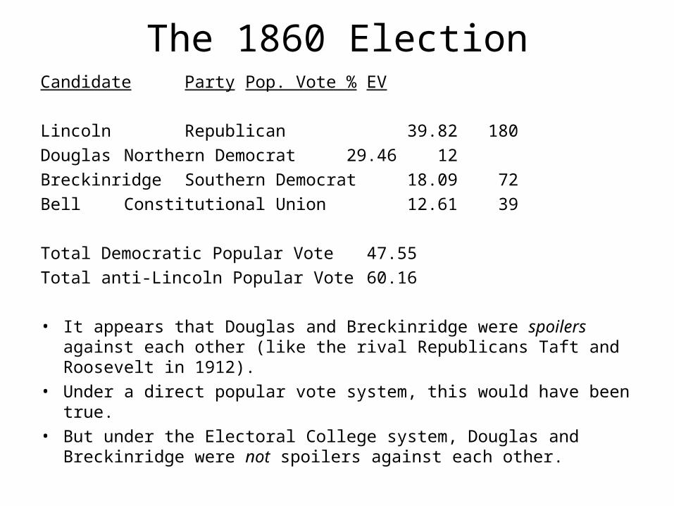
The 1860 ElectionCandidate Party Pop. Vote % EV

Lincoln Republican 39.82 180

Douglas Northern Democrat 29.46 12

Breckinridge Southern Democrat 18.09 72

Bell Constitutional Union 12.61 39

Total Democratic Popular Vote 47.55

Total anti-Lincoln Popular Vote 60.16

• It appears that Douglas and Breckinridge were spoilers against each other (like the rival Republicans Taft and Roosevelt in 1912).

• Under a direct popular vote system, this would have been true.• But under the Electoral College system, Douglas and Breckinridge

were not spoilers against each other.

A Counterfactual 1860 Election• Suppose the Democrats could have held their Northern

and Southern wings together and won all the votes captured by each wing separately.– Suppose further that it had been a Democratic vs. Republican straight

fight and that the Democrats had also won all the votes that went to Constitutional Union party.

– And for good measure suppose that the Democrats had won all NJ electoral votes (which for peculiar reasons were actually split between Lincoln and Douglas).

• Here is the outcome of the counterfactual 1860 election:

Party Pop. Vote % EV

Republican 39.82 169Democratic 60.16 134

• We will return to the 1860 election.

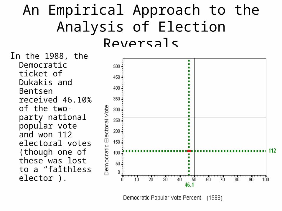
An Empirical Approach to the Analysis of Election Reversals

In the 1988, the Democratic ticket of Dukakis and Bentsen received 46.10% of the two-party national popular vote and won 112 electoral votes (though one of these was lost to a “faithless elector”).

Uniform Swing AnalysisOf all the states that Dukakis carried,

he carried Washington (10 EV) by the smallest margin of 50.81%.

If the Dukakis popular vote of 46.10% were (hypothetically) to decline by 0.81% uniformly across all states (to 45.29%), WA would tip out of his column (reducing his EV to 102).

Of all the states that Dukakis failed carry, he came closest to carrying Illinois (24 EV) with 48.95%.

If the Dukakis popular vote of 46.10% were (hypothetically) to increase by 1.05% uniformly across all states (to 47.15%), IL would tip into his column (increasing his EV to 136).

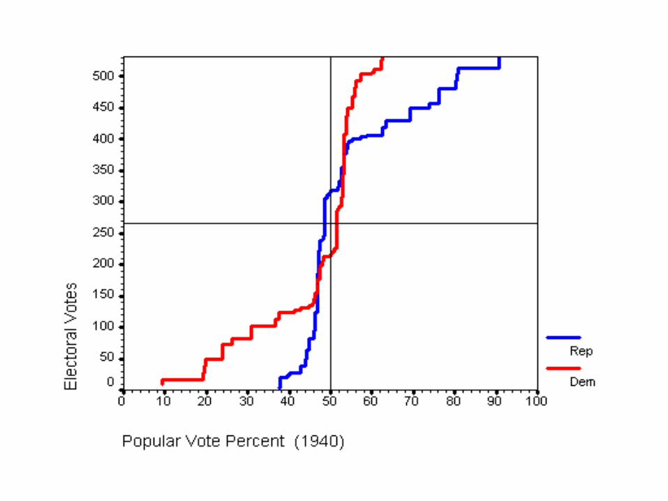
The PVEV Step Function for 1988

PVEV and Election Reversals

Zoom into Critical Region: Reversal Interval from 50.00% to 50.08%

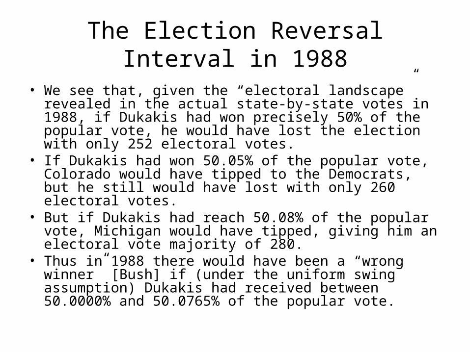
The Election Reversal Interval in 1988

• We see that, given the “electoral landscape” revealed in the actual state-by-state votes in 1988, if Dukakis had won precisely 50% of the popular vote, he would have lost the election with only 252 electoral votes.

• If Dukakis had won 50.05% of the popular vote, Colorado would have tipped to the Democrats, but he still would have lost with only 260 electoral votes.

• But if Dukakis had reach 50.08% of the popular vote, Michigan would have tipped, giving him an electoral vote majority of 280.

• Thus in 1988 there would have been a “wrong winner” [Bush] if (under the uniform swing assumption) Dukakis had received between 50.0000% and 50.0765% of the popular vote.

First Source of Possible Election Reversals

• This PVEV visualization makes it evident that there are two distinct ways in which election reversals may occur.

• First, an election reversal may occur as a result of the (non-systematic) “rounding error” (so to speak) necessarily entailed by the fact that the PVEV function moves up and down in discrete steps. – In this event, a particular electoral landscape may allow a wrong

winner of one party only but small perturbations of that landscape would allow a wrong winner of the other party.

• The 1988 chart (and similar charts for all recent elections [including 2000]) provides a clear illustration of a possible election reversal due to “rounding error” only.– So if the election had been much closer (in popular votes) and

the electoral landscape slightly perturbed, Dukakis might have been a wrong winner instead of Bush.

A Sample of 32,000 Simulated Elections Based on the 2004 Electoral Landscape

2000 vs. 1988

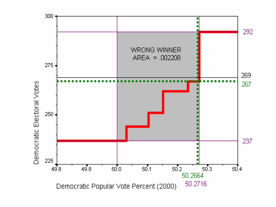
• The only real difference between the 2000 and 1988 (or 2004 and other recent) elections is that it was much closer.

– The election reversal interval was (in absolute terms) hardly larger in 2000 than in 1988:

• DPV 50.00% to 50.08% in 1988• DPV 50.00% to 50.27% in 2000

– But the actual DPV was 50.267%, i.e., (just) within the reversal interval.

Second Source of Possible Election Reversals

• Second, an election reversal may occur as result of (systematic) asymmetry or bias in the general character of the PVEV function. – In this event, small perturbations of the electoral

landscape will not change the partisan identity of potential wrong winners.

• In times past (e.g., in the New Deal era and earlier), there was a clear asymmetry in the PVEV function that resulted largely from the electoral peculiarities of the old “Solid South,” in particular,– its overwhelmingly Democratic popular vote

percentages, combined with– its strikingly low voting turnout.

Two Distinct Sources of Bias in the PVEV

• Asymmetry or bias in the PVEV function can results from two distinct phenomena:

• distribution effects.• apportionment effects; and

– Either effect alone can produce a reversal of winners, and they can either reinforce or counterbalance each other.

Apportionment Effects• A perfectly apportioned districted electoral system is one

in which each state’s electoral vote is precisely proportional to its popular vote in every election (and apportionment effects are thereby eliminated).

• It follows that, in a perfectly apportioned system, a party (or candidate) wins X% of the electoral vote if and only if it wins states with X% of the total popular vote.– Note that this say nothing about the popular vote margin by

which the party/candidate wins (or loses) states.– Therefore this does not say that the party wins X% (or any other

specific %) of the popular vote.

• An electoral system cannot be perfectly apportioned in advance of the election (in advance of knowing the popular vote in each state).

Apportionment Effects (cont.)• In highly abstract analysis of its workings, Alan Natapoff

(an MIT physicist) largely endorsed the workings Electoral College (particularly its within-state winner-take-all feature) as a vote counting mechanism but proposed that each state’s electoral vote be made precisely proportional to its share of the national popular vote.– This implies that

• electoral votes would not be apportioned until after the election, and• would not be apportioned in whole numbers.

– Such a system would eliminate apportionment effects from the Electoral College system (while fully retaining its distribution effects).

– Reversal of winners could still occur under Natapoff’s perfectly apportioned system.

– Natapoff’s perfectly apportioned EC system would create perverse turnout incentives in “non-battleground” states.

Alan Natapoff, “A Mathematical One-Man One-Vote Rationale for Madisonian Presidential Voting Based on Maximum Individual Voting Power,” Public Choice, 88/3-4 (1996).

Imperfect Apportionment• The U.S. Electoral College system is (substantially)

imperfectly apportioned, for many reasons. – House (and electoral vote) apportionments are anywhere from

two (e.g., 1992) to ten years (e.g., 2000) out of date.– House seats (and electoral votes) are apportioned on the basis

of total population, not on the basis of• the voting age population, or• the voting eligible population, or• registered voters, or• actual voters in a given election.• All these factors vary considerably from state to state (or district to

district).

– House seats (and electoral votes) must be apportioned in whole numbers and therefore can’t be precisely proportional to anything.

– Small states are guaranteed a minimum of three electoral votes.

Imperfect Apportionment (cont.)

• Similar imperfections apply (in lesser or greater degree) in all districted systems.

• Imperfect apportionment may or may not bring about bias in the PVEV function.– This depends on the extent to which states (districts)

having greater or lesser weight than they would have under perfect apportionment is correlated with their support for one or other candidate or party.

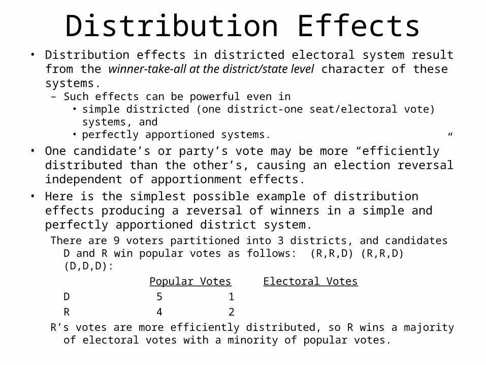
Distribution Effects• Distribution effects in districted electoral system result from the

winner-take-all at the district/state level character of these systems.– Such effects can be powerful even in

• simple districted (one district-one seat/electoral vote) systems, and• perfectly apportioned systems.

• One candidate’s or party’s vote may be more “efficiently” distributed than the other’s, causing an election reversal independent of apportionment effects.

• Here is the simplest possible example of distribution effects producing a reversal of winners in a simple and perfectly apportioned district system.There are 9 voters partitioned into 3 districts, and candidates D and R win

popular votes as follows: (R,R,D) (R,R,D) (D,D,D):

Popular Votes Electoral Votes

D 5 1

R 4 2

R’s votes are more efficiently distributed, so R wins a majority of electoral votes with a minority of popular votes.

The 25%-75% Rule• What is the most extreme logically possible example of a

“wrong winner” in perfectly apportioned system?• One candidate or party wins just over 50% of the popular

votes in just over 50% of the (uniform) districts or in non-uniform districts that collectively have just over 50% of the electoral votes.– These districts also have just over 50% of the popular

vote (because apportionment is perfect).• The winning candidate or party therefore wins just over

50% of the electoral votes with just over 25% (50+% of 50+%) of the popular vote and the other candidate with almost 75% of the popular vote loses the election.

• The elections reversal interval is (just short of) 25 percentage points wide.

• If the candidate or party with the favorable vote distribution is also favored by imperfect apportionment, the reversal interval could be winners could be even more extreme.

Distribution Effects (cont.)

• The Pure Proportional Plan for the Electoral College would entirely eliminate distribution effects.

• Election reversal could still occur due to apportionment effects– The reversals would favor candidates who do

exceptionally well in small and/or low turnout states).

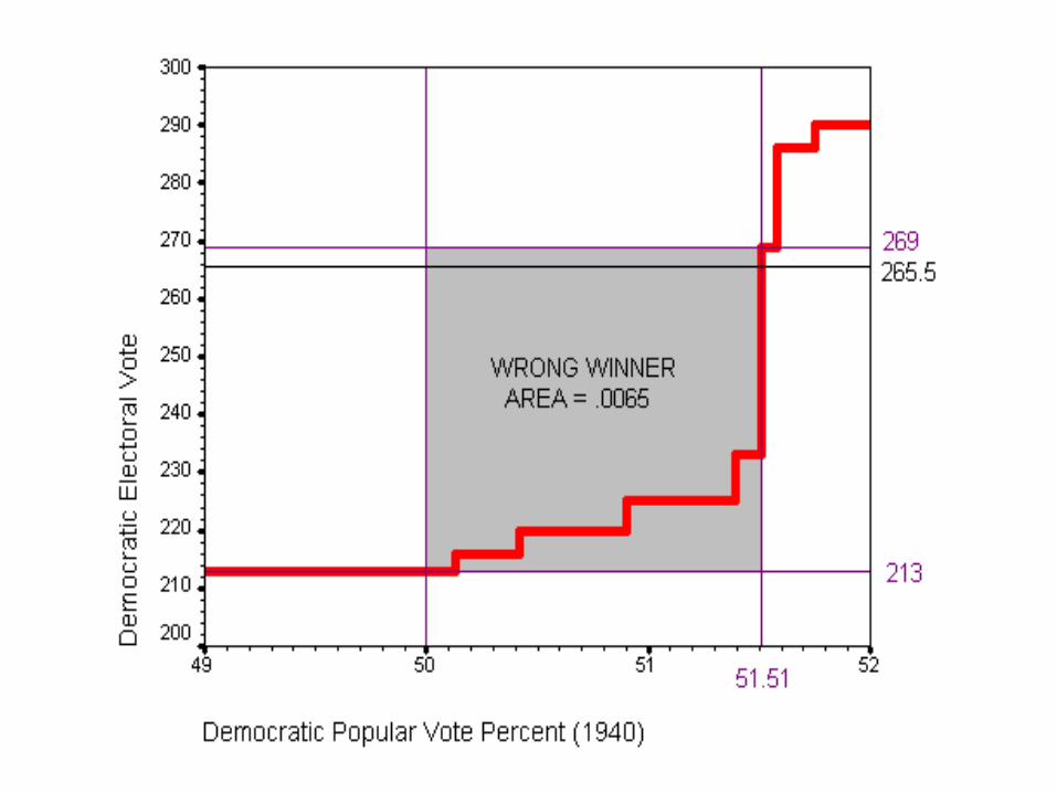
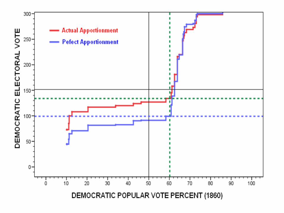
Apportionment vs. Distribution Effects in 1860

• The 1860 election was based on highly imper-fect apportionment.– The southern states (for the last time) benefited from

the 3/5 compromise pertaining to apportionment.– The southern states had on average smaller popula-

tions than the northern states and therefore benefited disproportionately from the small state guarantee.

– Even within the free population, suffrage was more restricted in the south than in the north.

– Turnout among eligible voters was lower in the south than the north.

Apportionment vs. Distribution Effects in 1860 (cont.)

• But all these apportionment effects favored the south and therefore the Democrats.

• Thus the pro-Republican reversal of winners was entirely due to distribution effects.– The magnitude of the reversal of winners in 1860

would have been even greater in the absence of the countervailing apportionment effects.

• If the most salient characteristic of the Electoral College is that it may produce election reversals, one’s evaluation of the EC may depend on whether one thinks Lincoln should have been elected President in 1860.

Supplementary Slides

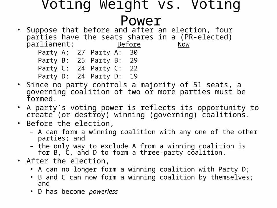
Voting Weight vs. Voting Power• Suppose that before and after an election, four parties have the

seats shares in a (PR-elected) parliament: Before Now

Party A: 27 Party A: 30Party B: 25 Party B: 29Party C: 24 Party C: 22Party D: 24 Party D: 19

• Since no party controls a majority of 51 seats, a governing coalition of two or more parties must be formed.

• A party’s voting power is reflects its opportunity to create (or destroy) winning (governing) coalitions.

• Before the election,– A can form a winning coalition with any one of the other parties; and– the only way to exclude A from a winning coalition is for B, C, and D to

form a three-party coalition.• After the election,

• A can no longer form a winning coalition with Party D;• B and C can now form a winning coalition by themselves; and• D has become powerless

Can Electoral Vote Apportionment Equalize Individual Voting Power?

• The question arises of whether electoral votes can be apportioned so that (even while retaining the winner-take-all practice) the voting power of individuals is equalized across states?

• One obvious (but constitutionally impermissible) possibility is to redraw state boundaries so that all states have the same number of voters (and electoral votes).– This creates a system of uniform representation.

Methodological Note: since the following chart compares voting power under different apportionments, voting power must be expressed in absolute (rather than rescaled) terms.

Individual Voting Power when States Have Equal Population (Versus Apportionment Proportional to Actual Population)

Uniform Representation

• Note that equalizing state populations not only:– equalizes individual voting power across states, but also– raises mean individual voting power, relative to that under

apportionment based on the actual unequal populations.• While this pattern appears to be typically true, it is not invariably

true,– e.g., if state populations are uniformly distributed over a wide range.

• However, individual voting power still falls below that under direct popular vote.– So the fact that mean individual voting power under the Electoral

College falls below that under direct popular vote • is not due to the fact that states are unequal in population and

electoral votes, and• is evidently intrinsic to a two-tier system.

Van Kolpin, “Voting Power Under Uniform Representation,” Economics Bulletin, 2003.

Electoral Vote Apportionment to Equalize Individual Voting Power (cont.)

• Given that state boundaries are immutable, can we apportion electoral votes so that (without changing state populations and with the winner-take-all practice preserved) the voting power of individuals is equalized across states?

• Yes (at least to close approximation), electoral votes can be apportioned by applying the Penrose Square Root Rule in reverse (as an engineering principle, rather than as a descriptive law):– Individual voting power is equalized when electoral votes are

apportioned so that state voting power is proportional to the square root of state population.

• But such Penrose Apportionment is tricky, because what must be made proportional to population is not electoral votes (what we directly apportion) but state voting power (a consequence of the apportionment of electoral votes).

(Approximately) Equalized Individual Voting Power

EV Apportionment to Equalize VP (cont.)

• These two methods of apportionment that equalize individual voting power equalize it at (essentially) the same level, namely– 0.00005785 (vs. 0.00007215 for direct popular vote).

• If the Penrose square root rule is used but apportion-ment of electoral votes must be in whole numbers,– individual voting power is imperfectly equalized

(especially among small state voters), and– mean individual voting power is reduced ever so

slightly (to 0.00005784).

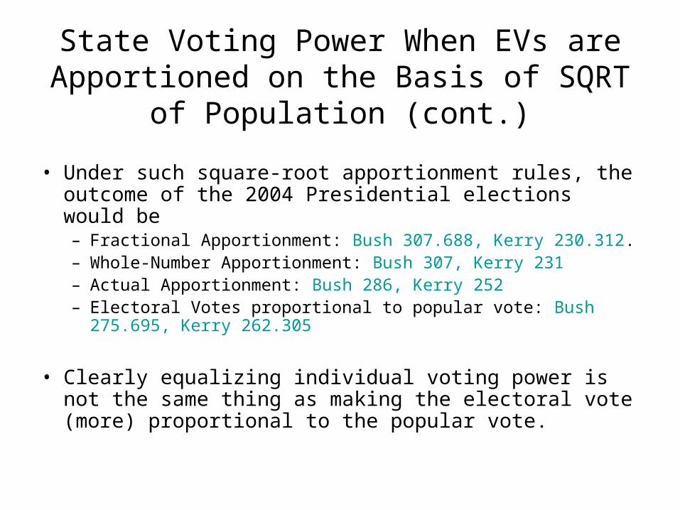
State Voting Power When EVs are Apportioned on the Basis of SQRT of

Population (cont.)

• Under such square-root apportionment rules, the outcome of the 2004 Presidential elections would be– Fractional Apportionment: Bush 307.688, Kerry 230.312.– Whole-Number Apportionment: Bush 307, Kerry 231– Actual Apportionment: Bush 286, Kerry 252– Electoral Votes proportional to popular vote: Bush 275.695,

Kerry 262.305

• Clearly equalizing individual voting power is not the same thing as making the electoral vote (more) proportional to the popular vote.

Election Reversals in Bernoulli Elections• Bernoulli elections

– clearly do not provide a good model of actual elections (as critics of the Banzhaft voting power measure regularly point out), but

– they may provide a neutral baseline for comparing the proclivity of different voting rules to produce election reversals.

• Given about 20 or more uniform districts (e.g., states with equal populations/numbers of voters), previous simulations have shown that election reversals occur about 20.4% of the time.

Feix, Marc R., Dominique Lepelley, Vincert R. Merlin, and Jean-Louis Rouet, “The Probability of Conflicts in a U.S. Presidential Type Election,” Social Choice and Welfare, 2004.

• In Bernoulli election samples of n = 32,000, rate of election reversals:Existing EV apportionment: 22.2% + 0.8% EV tieHouse only EV apportionment: 23.8% + 0.8% EV tiePrecisely proportional EV: 23.8%

Election Reversals in Bernoulli Elections (cont.)• Under the Pure and Modified District Plans, election reversals may

occur at the state level as well as the national level (though only the latter ultimately “matters”).

• In Bernoulli election samples of n = 16,000, rate of national election reversals:Pure District Plan 20.9% + 3.8% EV tiesModified District 16.5% + 2.5% EV ties

• At the state level, clear election reversals (other than EV ties, which are very likely in states with an even number of electoral votes) occur about • about 20% of the time in the largest states and less in smaller ones

under the Pure District Plan, and• About 12% of the time in the largest states and less is smaller ones

under the Modified District Plan.• The 2 EV statewide bonus reduces the incidence of reversals (as is

the clear intention of the National Bonus Plan).• It is impossible for reversals to occur in states with 3 or 4 electoral

votes.

The Original Gerrymander

Some Recent Gerrymanders

Closer to Home