,

OPTIMAL FILTERING APPLIED TOTHE VACUUM ARC REMELTING PROCESS

Rodney L. Williamson,+ Joseph J. Beaman$ and David K. Melgaardt

‘Liquid Metals Processing LabSandia National Laboratories

Albuquerque, New Mexico 87185-1134

‘Mechanical Engineering DepartmentUniversity of TexasAustin, Texas 78712

Abstract

Optimal estimation theory has been applied to the problem of estimating process variablesduring vacuum arc remelting (VAR), a process widely used in the specialty metals industry tocast large ingots of segregation sensitive and/or reactive metal alloys. Four state variables wereused to develop a simple state-space model of the VAR process: electrode gap (G), electrodemass (M), electrode position (X) and electrode melting rate (R). The optimal estimator consistsof a Kahnan filter that incorporates the model and uses electrode feed rate and measurementbased estimates of G, M and X to produce optimal estimates of all four state variables.Simulations show that the filter provides estimates that have error variances between one andthree orders-of-magnitude less than estimates based solely on measurements. Examples arepresented that verify this for electrode gap, an extremely important control parameter for theprocess.

DISCLAIMER

This repo~ was prepared as an account of work sponsoredby an agency of the United States Government. Neitherthe United States Government nor any agency thereof, norany of their employees, make any warranty, express orimplied, or assumes any legal liability or responsibility forthe accuracy, completeness, or usefulness of anyinformation, apparatus, product, or process disclosed, orrepresents that its use would not infringe privately ownedrights. Reference herein to any specific commercialproduct, process, or service by trade name, trademark,manufacturer, or otherwise does not necessarily constituteor imply its endorsement, recommendation, or favoring bythe United States Government or any agency thereof. Theviews and opinions of authors expressed herein do notnecessarily state or reflect those of the United StatesGovernment or any agency thereof.

DISCLAIMER

Portions of this document may be illegiblein electronic image products. Images areproduced from the best available originaldocument.

Introduction

Vacuum arq remelting (VAR) is a process used throughout the specialty metals industry for o$.~~

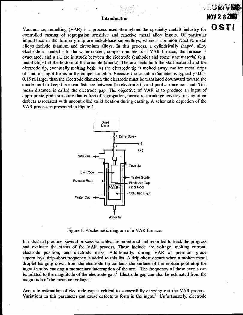
controlled casting of segregation sensitive and reactive metal alloy ingots. Of particularimportance in the former group are nickel-base superallo ys, whereas common reactive metalaIlo ys include titanium and zirconium alloys. In this process, a cylindrically shaped, alloyeleetrode is loaded into the water-cooled, copper crucible of a VAR furnace, the fi.umace isevacuated, and a DC arc is struck between the electrode (cathode) and some start material (e.g.metal chips) at the bottom of the crucible (anode). The arc heats both the start material and theeleetrode tip, eventually melting both. As the electrode tip is melted away, molten metal dripsoff and an ingot forms in the copper crucible. Because the crucible diameter is typically 0.05-0.15 m larger than the electrode diameter, the electrode must be translated downward toward theanode pool to keep the mean distance between the electrode tip and pool surface constant. Thismean distance is called the electrode gap. The objective of VAR is to produce an ingot ofappropriate grain structure that is free of segregation, porosity, shrinkage cavities, or any otherdefects associated with uncontrolled solidification during casting. A schematic depiction of theVAR process is presented in Figure 1.

L

DriveMcior

=(-~l-d-Pr-(+)

Fur

w 1“Crucible

Water Guide

Eleotr@ Gap

Ingct Pod

Solidified ingot

Waterln

Figure 1. A schematic diagram of a VAR furnace.

In industrial practice, several process variables are monitored and recorded to track the progressand evaluate the status of the VAR process. These include arc voltage, melting current,electrode positio~ and electrode mass. Additionally, during VAR of premium gradesuperalloys, drip-short frequency is added to this list. A drip-short occurs when a molten metaldroplet hanging down from the electrode tip contacts the surface of the molten pool atop theingot thereby causing a momentary interruption of the arc.* The frequent y of these events canbe related to the magnitude of the electrode gap. 2 Electrode gap can also be estimated horn themagnitude of the mean arc voltage.3

Accurate estimation of electrode gap is critical to successfully carrying out the VAR process.Variations in this parameter can cause defects to form in the ingot.4 Unfortunately, electrode

gap estimates based on arc voltage and drip-short frequency are very noisy and averaging overtens of seconds is required to obtain sufficiently accurate information. Melt rate estimates basedon electrode weight measurements are worse still. It is common practice in many industrial meltshops to estimate melt rate from the slope of a twenty minute sliding window of electrode massdata.

The problem of noisy estimates directly impacts the problem of process control. Commandedelectrode velocity is dependent on average drip-short frequency or arc voltage for feedback.This makes for a highly damped electrode drive system that is unable to react to processtransients and upsets in a timely fashion. Melt rate estimates are either so noisy or so highlydamped that active current control using melt rate estimates for feedback is not practical.Common industrial practice requires that the melting current be controlled to a constan~ steady-state value characteristic of a material and electrode/ingot size. Occasionally a shop will usemeasured melt rate to trim around the steady-state current.

This paper focuses on the development of a VAR process filter that facilitates acquiringaccurate, instantaneous variable estimates for the purpose of process monitoring and electrodegap control. A dynamic model of electrode gap is developed and a discrete state-space model ofthe process is formed in terms of four state variables: electrode gap (G), electrode mass (M),

electrode position (X), and electrode melting rate (R= M). The single input to the system is

electrode drive velocity, X, written as V below. An optimal estimator is then developed usingKalman filter theory. The performance of the filter is evaluated using simulations. Electrode gapdata are presented from actual laboratory and industrial tests to verify the performanceimprovements predicted by the simulations.

Filter Development

The electrode gap dynamics are described by the following differential equation:

G=iel–hhg–v. (1)

This equation states that, over a vanishingly short time interva~ the change in gap equals the

change in electrode length ( iel ) due to melting less the change in ingot height ( htig ) due to

mold filling and the change in electrode position due to its being driven down. The f~st term onthe right can be found by assuming that liquid metal leaves the surface as soon as it forms and

that the electrode tip surface is flat with an area given by && where & is the room temperaturecross-sectional area and & accounts for the effects of thermal expansion. The resultingexpression is .

ie, =R

l%q&Ae

where pli~ is the liquid metal allo y densit y.

(2)

The second term in Eq. (1) is directly related to the f~st since the ingot is formed from materialmelted off the electrode. The relationship is complicated by the fact that the ingot is beingcooled and its density is a function of both ingot height and radial ingot position. In steady-state,it is assumed that the change in ingot height with time can be described by

,

(3)

where K is a constant factor that corrects the room temperature electrodehngot area ratio (oftencalled the fill ratio) for thermal effects. This is born out in practice where it is found that, understeady-state melting conditions, a linear drive speed is required to achieve a constant electrodegap.

Substituting Eq.’s (2) and (3) into Eq. (1) gives the following expression for the time dependentgap behavio~

(hG=J- ~–- –V=OR-V (4)~fiqe Ae Ai

In practice, an average value for ct is estimated from melt data for a particular process.

Using the state-space formalism, the discrete time VAR process can be described by a matrixequation of the form

Xn+l = Axn +Bun +NwR (5)

where A, B and N are the transition, input, and process noise matrices, respectively, x is thestate vector consisting of the four variables listed in the Introduction, and u is the control input“vector” consisting only of the electrode drive speed. N operates on w, a vector characterizingthe uncertainty in the inputs that drive the plant as well as uncertainty in the plant itself. Theseterms constitute the process noise. It is assumed that each component of w can be represented indiscrete time by a white sequence with zero-mean. In other words, the process noise isuncorrelated and unbiased. The subscripts in Eq. (5) refer to time-steps in the discrete timesystem. A, B and N are determined by considering the dynamics of the VAR process.

As seen above, changes in electrode gap are directly related to the relative velocities of thegrowing ingot and moving, melting electrode. Converting Eq. (4) to discrete time andaccounting for process uncertainty, the electrode gap dynamics are described by

Gn+l =Gn +CYRnT-VnT-WXn(V) +ROTwan (6)

where T is the sample time, ~ is the nominal melt rate, w x, (v) quantifies the uncertainty in

electrode. position due to uncertain y in the electrode drive velocity, and w ~~ quantxles

uncertainty in ct. This uncertainty stems from surface variations in both the electrode andcrucible, variation in the electrode cross-sectional area due to voids, and fluctuating temperaturedistributions in both the electrode and ingot.

The dynamics of the electrode mass are directly related to melt rate by

Mn+l =Mn–RnT. (7)

In words, the mass at twl is the mass at t. less what melted off in the time interval T.

,

Position changes are tied directly to velocity according to

Xn+l =Xn +vn’I’+wxn(v). (8)

The position at t.+l is just the position at t. plus the distance moved in the last time stepcorrected for the uncertainty in the electrode drive velocity.

Finally, the formulation assumes that the melt rate is a random variable with no driving term sothat the dynamics are simply described by

R~+l =R~ +WRn (9)

where w R~ quantfles the uncertain y in the melt rate. Note that Eq; (9) does not guarantee that

the melt rate will remain indefinitely at its initial value. Indeed, over a time period consisting ofmany time steps it will randomly walk away from that value, the maximum step size of the walkbeing determined by the uncertainty. In practice, the plant behavior differs from this becauseone attempts to drive the melt rate with melting current. Insofar as the development of the falteris concerned, this is irrelevant so long as one has correctly accounted for the process andmeasurement noise sources.5

The development has assumed a straight electrode and crucible: & and Ai are not functions oftime. However, it is often the case that melting is performed with both tapered electrode andcrucible for the simple reason that a tapered casting is easier to remove from the mold. Becauseof this, it is not uncommon for et to vary linearly by 10-20% over the duration of a VAR melt.One may easily account for this non-random error by modeling the time-dependent behavior ofa, an exercise that adds complication to the filter development but nothing conceptually to theway it works and performs. For this reason, the more complicated formulation is not given here.However, a simple method of including this feature in the model is to linearize Eq. (4) about thenominal values (W,~,Vo), and then add a new state variable Au=ct-@ where cx is now afunction of the amount of material melted.

Making appropriate substitutions, Eq. (5) can be written as

(lo)

which relates the electrode gap, mass, position and melt rate at tW1 to their values at t~ givenboth deterministic and random inputs. A, B and N can now be derived from inspection of Eq.’s(6)-(10). They are

[1

100ctT

O1O–TA=

0010

0001

(11)

,,

-T

o

T

o 1

B=

and

N=

–1

o

1

0

ROT O

00

00

01

(12)

(13)

Besides state variables and inputs, the system is also characterized by outputs, some, or al~ ofwhkh can be measured. The outputs for this system are taken to be electrode gap, mass andposition. The output equation is then given by

[1[Gn

GnMn

Mn =CXn

XnRn

Again by inspection, it is seen the C must be given by

[11000

C=o loo.

0010

Assuming that all outputs can be measured, the measurements at t. are modeled by

IGn

Mn‘n =C

Xn

Rn [1VG

n

+ VMn

Vxn

(14)

(15)

(16)

where the elements of the column vector, Vn, characterize the measurement noise (assumedwhite with zero mean) present in the gap, mass and position measurements.G

Given the process and measurement models embodied in Eq.’s (6)-(16), a Kalman filter (oroptimal state observer) can be constructed using known methods the details of which arepresented in standard texts on modern control system design.7 The equation for the filter indiscrete time is

in+l = Afin +Bun +M~(zn –Ckn) (17)

where & B and C are as defined above for the plant, and a “hat” over a variable denotes an

estimate. in +1 is the predicted system state at t.+l estimated from measurements and the

estimated state at tn. The Kahnan matrix, MK, is chosen so as to minimize the error covarianceof the estimated variables relative to their true values and can be derived from the steady-stateprocess and measurement noise covariances. There are as many columns in MK as measuredsystem outputs, and as many rows as state variables. In the present application, MK is a 4x3matrix. Off-diagonal elements arise because of couplings between the variables. For example,

d is related to the measured values of all three outputs since WX,(V1 is a position term and

melt rate is directly related to electrode mass (Eq. (6)). Therefore, the fwst row of MK containsall non-zero values. On the other hand, there is no measurement for a and, thus, nocorresponding element in MK. The difference term in Eq. (17), called the innovation, goes tozero only in the case where the measurements are noise free and match perfectly the modelpredictions. In this situation, the future state is perfectly predicted from the present state by thesystem model, and all estimated values exactly equal the actual values. This situation neverholds in practice.

The Kahnan filter produces estimates of the future state and current outputs. These estimates aretied to process and measurement noise through a model of the system according to an optimalweighting scheme. If the process inputs and parameters are known with a high degree ofprecision relative to the measured outputs, the estimates will not be greatly influenced by themeasurements, i.e. the filter ‘knows” that the measurements cannot be trusted. In this case, theelements of MK will be very small and the estimator will be model based. The filter simplytakes advantage of the fact that the state of the system is nearly completely determined by thephysical constraints placed on it by the inputs and process variables coupled with knowledge ofthe previous state. On the other hand, if relatively exact measurements are available, theestimator will weigh them more heavily than the process model and the falter will bemeasurement based. Obviously, if all the outputs can be measured exactly, they do not need tobe estimated.

Filter Performance

A block diagram of the VAR process model coupled to the Kalman filter is shown in Figure 2.A computer program was written using the Matlab~ programming language (The Math Works,Inc., Natick, MA) for the purpose of evaluating the improvement in the Kalman estimatedoutputs relative to the measured values. The simulations assume a 0.432 m (17 in.) diameterelectrode being melted into 0.508 m (20 in.) diameter ingot at a nominal melt rate of 0.060 kg/s(476 lb/hr) and electrode drive speed of -1.8x10-5 m/s (2.6 in./hr). These parameters are typicalfor VAR of Allo y 718. ot is taken to be 2.94x104 mlkg based on experience melting this typeand size material at this melt rate. This number is about 9% larger than what would be obtainedby simply setting E=K=l in the expression for U. In the simulations, a sample time of 4 secondswas used.

The random sequences characterizing the process and measurement noise terms are eachdescribed by a standard deviation and variance. In practice these are determined through processcharacterization. For the simulations, OX(W was set to 2.0x104 m corresponding to anuncertainty in V of 5.0x10-7 m/s, and @ was set to 1.0x1C)4 kg/s. ~a was estimated to be about5% of the nominal value, or 1.3x10-5 fig, by assuming that the electrode and crucible radiivary by only 4.001 m over the duration of the melt, that the density is known to within *1OOkg/m3, and that the other parameters are constant. The measurement noise (standard deviation)terms were set to 5X10-3m, 1 kg and 10-3 m for vG, vM and Vx, respectively. These are believedto be typical of the measurement capabilities available on many VAR furnaces in industry.,

I , 8----------------------------------------

L GiiG------”\i;’-------”\

.. ------ -------- ----------- ----------- ------- . .

Figure 2. A block diagram showing the VAR process coupled to the Kalmanfalter. The Process Model replaces the actual plant in the simulations.

Figure 3 shows a plot of G and 6 (its filtered value) resulting from a 5000 s simulation for anopen-loop system (no feedback). V was set to 1.755 x10-5 m/s in this simulation. The figure

demonstrates that G (Ge) tracks the “true” gap (G) very well. Drift in the gap from the nominalvalue of 0.01 m is due to the uncertainties in the system. Because of the random errors in thesystem, the difference between the gap and its nominal value follows a random walk trajectory.

0.0115

0,011

0.0105

0.01

0.0095

Emll“’’’’’’’(’’’’’’’’”1

I I I I

o 1000 2000 3000 4000 5000

Time (S)

Figure 3. Simulated open-loop estimation of electrode gap.

~ is shown in Figure 4 plotted with the simulated measurement based estimate of electrodegap. The noise reduction achieved through Kalman filtering is readily apparent. This effect isseen in Table I, where error variances are tabulated for the measured and correspondingestimated outputs of the simulation. Note that the variances in the simulated measurementsapproximately equal the squares of the specifkd measurement noise terms, as required. Also

note that the error variance in & may change by as much as a factor of two from simulation tosimulation whereas the error variances for the other estimates are more stable.

0.03

0.0.25

0.02

0.015

0.01

0.005

0

-0.005

-0.01

1- J

1 1 I 1

0. 1000 2000 3000 4000 5000

Tittw(S)

Figure 4. Simulated measured (Gz) and filtered (Ge) electrode gap.

Table I. Variances of measured (-) and filtered (A) variables.

U-w@ – G) 2.5x10-5

Vizr.(d – G) 1.3X10-8

~Var.(A7 –M) 0.99

F=t--iVar.(i – x) 2.3x10-Y

Gap estimation was found to be sensitive to either increases or decreases in the gapmeasurement error indicating that the estimator, as defined, is neither completely model- normeasurement based. However, estimates are insensitive to measurement error once it has beenincreased beyond about 4.1 m, indicating that the estimator is model based under thesemeasurement conditions. In other words, if one cannot measure gap to better thfi _W.1 m underthese’ process conditions, the measurement is irrelevant to gap estimation. On the other hand, theestimator is completely measurement based with respect to gap measurement at a measurementresolution of&5x104 m. At this resolution, the estimator becomes superfluous.

Simulation shows that accurate mass measurements (+1 kg) are beneficial for electrode gapestimation. However, improvements beyond this have little effect. Increasing the measurementerror adversely affects the gap estimate up to about HO kg. Under the process conditionsinvestigated, one might as well have no mass measurement at all if the error is increased beyondthis value. Thus, with respect to electrode mass measurement, the estimator is model basedbeyond a measurement error of about 90 kg and measurement based at measurement errorsless than Al kg.

Simulation further indicates that gap estimation is not improved significantly by improving theresolution of the position measurement under the simulation conditions investigated. One mustresist concluding from this that exact position measurements are of little intrinsic value to gapestimation. This depends on the uncertainties characterizing thes ystem. For example, if one has

poor ram control, the error covariance in ~ may be significantly reduced by increasing theposition measurement resolution. In genera~ complete system characterization is requiredbefore one can decide how to improve the estimation of important process variables.

Verification of Simulation Results for Electrode Gap

The simulations were performed for hypothetical situations considered to be typical of actualVAR processes. It is appropriate to show some sample data to verify that significant reductionsin the noise characteristics of parameter estimates can be realized in actual practice by usingKahnan filtering. As pointed out in the introduction, accurate electrode gap estimation isnecessary for successful control of the VAR process. Electrode gap data from two test melts areshown below. Each example includes measurement based and Kahnan faltered estimates ofelectrode gap. It should be noted that the falters used in the two examples differ in their detailsfrom the one developed above. This is because the tests involved estimation of additionalcontrol variables important for controlling aspects of the process not discussed in this paper.Information concerning these tests and the estimators they employed is unavailable forpublication at this time. However, the dynamics described by Eq.’s (6)–(9) are captured in thesemore general filters and the examples are appropriate to illustrate the improvements in noisereduction realized by Kalman filtering.

The data shown in Figure 5 were acquired during VAR of 0.203 m diameter Alloy 718electrode into 0.254 m diameter ingot on the VAR i%mace at Sandia National Laboratories.Neither the electrode nor the crucible were tapered. Because there is no mass transducer (loadcell) on this i%mace, the measurement uncertainty is infinite for electrode mass. Melt ratederived from position measurements during the interval shown was estimated to be 0.040M.002kg/s and the drive speed noise was similar to that used for the simulations. A high resolutionencoder is mounted on the furnace so that the resolution in X was 10-5 m. The noise variance inthe drip-short based measurement of G was 2.6x10-5 m2. In comparison, the variance in theKalman filter estimate of G was 5. 1X10-9m2 giving a signal to noise improvement of about 70.Drive speed control decisions were made every two seconds based on the filtered estimates. The

,

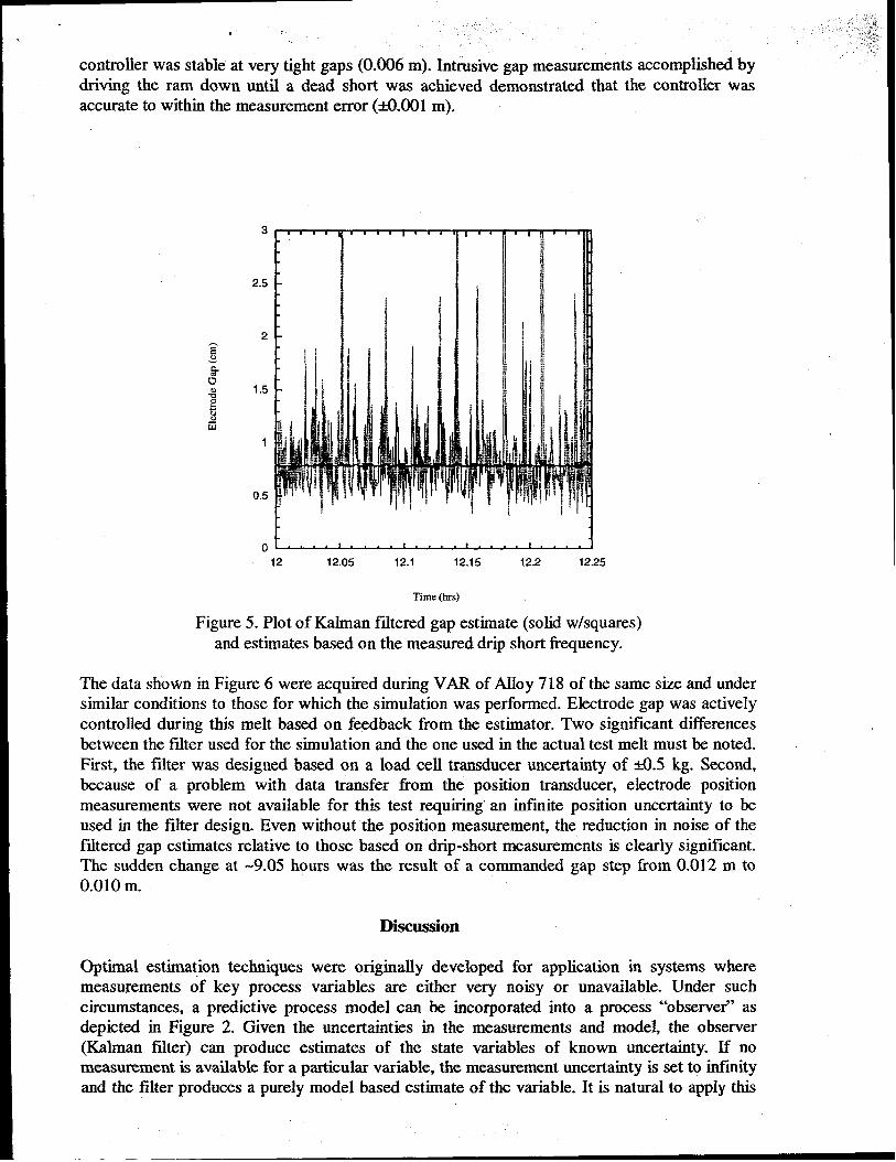
controller was stable at very tight gaps (0.006 m). Intrusive gap measurements accomplished bydriving the ram down until a dead short was achieved demonstrated that the controller wasaccurate to within the measurement error (M.001 m).

3r—T—————

2.5

2

1.5

1

0.5

I

It

ol r t 1 I

12 12.05 12.1 12.15 122 1225

Time(hrs)

Figure 5. Plot of Kalrnan faltered gap estimate (solid w/squares)and estimates based on the measured drip short fkquency.

The data shown in Figure 6 were acquired during VAR of Allo y 718 of the same size and undersimilar conditions to those for which the simulation was performed. Electrode gap was activelycontrolled during this melt based on feedback from the estimator. TWO signiilcant differencesbetween the filter used for the simulation and the one used in the actual test melt must be noted.First, the filter was designed based on a load cell transducer uncertainty of A.5 kg. Second,because of a problem with data transfer from the position transducer, electrode positionmeasurements were not available for this test requiring’ an infinite position uncertainty to beused in the filter design. Even without the position measurement, the reduction in noise of thefaltered gap estimates relative to those based on drip-short measurements is clearly significant.The sudden change at -9.05 hours was the result of a commanded gap step tlom 0.012 m to0.010 m.

Discussion

Optimal estirna~ion tecluiques were originally developed for application in systems wheremeasurements of key process variables are either very noisy or unavailable. Under suchcircumstances, a predictive process model can be incorporated into a process “observer” asdepicted in Figure 2. Given the uncertainties in the measurements and mode~ the observer(Kalman filter) can produce estimates of the state variables of known uncertainty. If nomeasurement is available for a particular variable, the measurement uncertainty is set to infinityand the filter produces a purely model based estimate of the variable. It is natural to apply this

—

.* “’j>:x3

Y

“, .- .:.,::,,.,,

technology to estimating electrode gap in the VAR process where one encounters noisymeasurements that are often spoiled by common process disturbances.

3

2.5

2

1.5

1

0.5

0 1 .,...,...,.,...1.1#.6 8.8 9 9.2 9.4

lime (hrs]

Figure 6. Plot of Kalman filtered gap estimate (solid w/squares)and estimates based on the measured drip short Iiequency.

Given the noise inherent in drip-short and arc voltage data, it is to be expected that estimates ofelectrode gap based on these data will be highly uncertain after only a few seconds of dataacquisition. Often the uncertain y in the estimate exceeds the magnitude of the controlreference. However, given the process inputs and noise characteristics, and the last stateestimate, one can determine, based on physics alone, how much the gap could possibly havechanged during the last time step. It is this physics based limitation that the filter imposes on thegap measurement and, for this reason, this type of filtering is sometimes called “physicalfiltering.” Physical filtering constrains the estimate to be consistent with the physical situationas described by the model and the measurements. In the case of electrode gap, the filter requiresthat the estimated change from one time step to the next be consistent with the electrodevelocity and melting rate as described by Eq. 6 as well as the measurement based estimation.The relative weights of the two estimates are reflected in the elements of the Kahnan gainmatrix and depend on the process and measurement uncertainties.

Though the focus of this paper has been electrode gap estimation, it has been made clear that thefalter produces estimates of all state variables, including melt rate (Figure 2). Melt rate was notincluded as a measurement because of the difilculty involved with obtaining” it from electrodemass measurements as mentioned in the Introduction. This difficulty arises because of the noiseintroduced into the measurement based estimate by taking the derivative of the mass transduceroutput. Determining the slope over long time intervals (10-20 minute) of mass data helps withthe noise but introduces unacceptable lag into the estimate and effixtively “erases” short term

transients. The simple filter developed for this paper effectively addresses this issue and its usein an actuals ystem would, no doubt, result in a significant improvement in melt rate estimation.However, no experimental test involving this particular falter has been performed to confirmthis. The latest generation of VAR controllers developed by Sandia National Laboratories andthe Specialty Metals Process Consortium does, inde~ employ Kalman filtering to produceaccurate, relatively noise-free melt rate estimates, but the filtering’ relies on “asignflcantly morecomplex state-space model with respect to electrode melting dynamics. As a result, the melt rateestimate is affected by variables missing from Eq. (9) and the results are not germane to thisstudy. This more advanced technology is described in a disclosure recently submitted to theUnited States Patent OffIce and further information related to it is not yet available for externalpublication.

Conclusions

The following conclusions can be made from this work

1. Kahnan filtering provides a superior means of estimating electrode gap for VAR processcontrol. The estimates are significantly less noisy and provide the basis for improving both thestability and response of the control system.

2. The Kalman filter development described here provides a means of estimating electrodemelting rate that is not dependent on differentiating the load cell output. Hence, the estimatesare not heavily damped and are useful for electrode gap control purposes.

3. The error variance of the gap estimate could be affected by either increasing or decreasing thegap measurement uncertainty indicating that, under the process conditions of interest, theestimator was neither completely model based nor measurement based. Increasing themeasurement error beyond M. 1 m is equivalent to having no gap measurement at all.

4. An accurate electrode mass measurement is beneficial for electrode gap control up to anaccuracy of& 1 kg under the process conditions investigated. Increasing the mass measurementerror to &O kg is tantamount to having no mass data at all.

5. Increasing or decreasing the position measurement error has little effect unless one has poorram control. With poor ram contro~ accurate, precise position measurement is beneficial.

Acknowledgments

A portion of this work was supported by the United States Department of Energy underContract DE-AC04-94AL85000. Sandia is a multiprogram laboratory operated by SandiaCorporation, a Lockheed Martin Company, for the United States Department of Energy.Additional support was supplied by the Specialty Metals Processing Consortium

References

1. F. J. Zanner: h4etalL Trans. B, 1979, 10B, pp. 133-42.2. F. J. Zanne~ Metall. Trans. B, 1981, 12B, pp. 721-8;3. R.L. Williamson, F. J. Zanner, and S.M. Grose: MetalL And Mater. Trans. B,

841-53.997, 28B, pp.

4. D. K. Melgaard, R. L. Wfliamson and J. J. Beaman: JOM, 1998, VOL50(3), pp. 13-17.

5. Though this paper is focused on electrode gap dynamics and control, it is possible togeneralize the treatment to the dynamics of the VAR process as a whole, in which case it isessential to include the melt rate response to melting current.

6. The term “measurement” as used here means not only direct measurements but alsoderivations based on direct measurements. Thus, electrode gap is termed a measured variableeven though it must be calculated from drip-short frequency or voltage data.

7. See, for example, B. Friedland, Control System Design, An Introduction to State SpaceMethoa%, McGraw-Hill, Inc., New York, NY, 1986. Also, Applied Optimal Estimation, A.Gelb, cd., M.I.T. Press, Cambridge, MA, 1994.