“The wise are instructed by reason;ordinary minds by experience;the stupid, by necessity; andbrutes, by instinct.” -Cicero

“A man’s judgement is no better than his information.” - from Bits & Pieces

Laplace transformsIntroduction

Review of Complex Variables and Complex functions

Laplace transformation

Inverse Laplace transformation

Partial Fraction Expansion with MATLAB

Solving DEs

Assignments (start now)

Introduction

Tim e d o m a inu n kn o w n f(t), d /d t, D iff E q s

F re q u e n c y d o m a inu n kn o w n F (s ), A lg E q s

L a p lac eTra n s fo rm a tio n

S o lveA lge b ra icE q u a tio n s

F re q u e n c y d o m a inkn o w n F (s )

Tim e d o m a inkn o w n f(t)

S o lveD iffe re n tia lE q u a tio n s

In ve rs eL a p lac eTra n s fo rm

Review of Complex Variables and Complex functions

s j Re( )s Im( )s

2 2| |s 1tans

| | cos( ) sin( )s s s j s

?, ?

s j 2| |s ss

Review of Complex Variables and Complex functions

( ) ( , ) ( , )x yG s G G j | ( ) | ?

( ) ?

G s

G s

0 0

( ) ( )( ) lim lims s

d G s s G s GG s

ds s s

s j Limits are path dependent. Consider 2 paths.

0( ) lim yxs

GGd GG s j

ds

0( ) lim yxs j

GGd GG s j

ds j

Review of Complex Variables and Complex functions

Limits are path dependent. Consider 2 paths. If equal

y yx xG GG G

j j

Equating real and imaginary parts

,y yx xG GG G

Cauchy-RiemannConditions.

Only if these two conditions are satisfied, the function G(s) is analytic.

Review of Complex Variables and Complex functions

Points in the s plane at which the function G(s) is analytic are called ordinary points.Points in the s plane at which the function G(s) is not analytic are called singular points.Singular points at which the function G(s) or its derivatives approach infinity are called poles.Singular points at which the function G(s) equals zero are called zeros.If G(s) approaches infinity as s approaches –p and if the function G(s)(s+p)n, for n = 1, 2, 3, … has a finite, nonzero value at s = -p, then s=-p is called a pole of order n.If n = 1, the pole is called a simple pole.

Review of Complex Variables and Complex functions

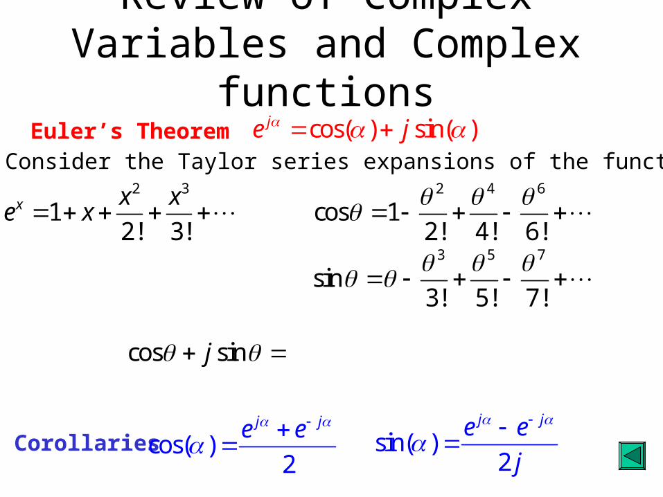
Euler’s Theorem cos( ) sin( )je j

Corollaries cos( )2

j je e

sin( )2

j je e

j

Proof: Consider the Taylor series expansions of the functions2 3

12! 3!

x x xe x

2 4 6

cos 12! 4! 6!

3 5 7

sin3! 5! 7!

cos sinj

Laplace Transformation 0

( ) ([ )]t st

te dtf t f t

L

0[1(

0, 01( ) ]) ( )

01,

1,

t st

te d

ttt

ttt

L

0 01( ) 1( )[ ]

t tst st

t tet t dt e dt

L

0

1t

st

t

es

1

lim 1stt e

s

1

s

Laplace Transformation 1

![ 1( )]

( )n at

n

AnAt e t

s a

L

( ) cos( )1( )

cos( )1(

,

[ ])

f t A t t

A t t

L 1( )2

j t j te eA t

L

1( ) 1( )2 2

j t j te eA t A t

L L

1 1

2 2

A A

s j s j

( )

2

s j s jA

s j s j

2 2

As

s

Laplace Transformation [ ( )] 1t L

Inverse Laplace Transformation3

( )( 1)( 2)

sF s

s s

Partial fraction Expansion.“Cover up Rule”

( )1 2

F ss

A B

s

2( ) 1( )t tf t e eA B t

3( 1) ( 1)

( 1)( 2) 1 2

s A Bs s

s s s s

3( 1)

( 2) 2

s BA s

s s

2

3

( 1)s

sB

s

2A

A:

3( 2) ( 2)

( 1)( 2) 1 2

s A Bs s

s s s s

3( 2)

( 1) 1

s As B

s s

1

3

( 2)s

sA

s

1B

B:

2( ) ( ) 1(12 )t tf t e e t

Laplace transform of a

derivative

( ) ( ) (0)d

L f t sF s fdt

Primes and dots are often used as alternative notations for the derivative.

Dots are almost always used to denote time derivatives.

Primes might denote either time or space derivatives.

In problems with both time and space derivatives, primes are space derivatives and dots are time derivatives.

Note: Lower case f indicates function of time. Upper case F indicates function of s.

(Multiplication by s) = (differentiation wrt time)

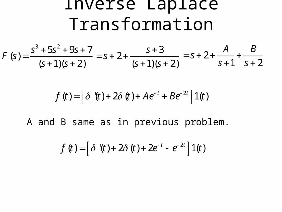
Inverse Laplace Transformation

3 25 9 7( )

( 1)( 2)

s s sF s

s s

3

2( 1)( 2)

ss

s s

2

1 2

A Bs

s s

2( ) '( ) 2 ( ) 1( )t tf t t t Ae Be t

2( ) '( ) 2 ( ) 2 1( )t tf t t t e e t

A and B same as in previous problem.

(Today’s date: 8/29/03) Assignment due next class period

• You will receive two pieces of paper– One has “Good” (not necessarily perfect)

responses to the quiz questions.– The other has a different response to the quiz

questions. These may or may not have errors on them. This page has your name on a label.

• Use the notes and the “Good” responses to make corrections on the quiz responses on the page with your name on it.

Inverse Laplace Transformation2

2

2 12( ) , 2 5 ( 1 2)( 1 2)

2 5

sF s s s s j s j

s s

2 12

( )( 1 2)( 1 2)

sF s

s j s j

( 1 2) ( 1 2)

A A

s j s j

(1 2) (1 2)( ) 1( )j t j tf t Ae Ae t

1 2

2 12

1 2s j

sA

s j

2( 1 2) 12

1 2 1 2

j

j j

1 2.5 j 1.19032.6926 je

(2 1.1903) (2 1.1903)( ) 2.6926 1( )t j t j tf t e e e t

1.19032.6926 jA e

( ) 5.3852 cos(2 1.1903) 1( )tf t e t t

Inverse Laplace Transformation2

3

2 3( )

( 1)

s sF s

s

2 31 ( 1) ( 1)

A B C

s s s

2 31 ( 1) ( 1)

A B C

s s s

23 3

3 2 3

2 3( 1) ( 1)

( 1) 1 ( 1) ( 1)

s s A B Cs s

s s s s

2( ) 1( )2

t t tCf t Ae Bte t e t

2 22 3 ( 1) ( 1)s s s A s B C 2 2

1 12 3 ( 1) ( 1)

s ss s s A s B C C

2

2

1

2 3s

dB s s

ds

12 2

ss

0

22

2

1

2 3s

dA s s

ds

2

1

2 2s

ds

ds

2

2( ) 2 1( )t tf t e t e t

Partial Fraction Expansion with MATLAB

Read Section 2-6Feel free to use MatLab to check your work.You will not have access to MATLAB on tests.

Solving DEs Laplace transforms are the primary tool used to solve DEs in control engineering.

ds

dtL

22

2

ds

dtLWhen initial

conditions are zero:

nn

n

ds

dtL

For non zero initial conditions

( ) ( ) (0)d

y t sY s ydt

L

2

2( ) ?

dy t

dt

L

3

3( ) ?

dy t

dt

L ( ) ?

n

n

dy t

dt

L

0( ) ?

tL f d

Solving DEs 3 2 0, (0) , (0)x x x x a x b

2 ( ) (0) (0) 3 ( ) (0) 2 ( ) 0s X s sx x sX s x X s 2 3 2 ( ) 3s s X s sa b a

2

3( )

3 2

sa b aX s

s s

3

( 1)( 2)

sa b a

s s

1 2

A B

s s

2( ) 1( )t tx t Ae Be t

1

3

2 s

sa b aA

s

2b a

2

3

1 s

sa b aB

s

B b a

2(2 ) ( ) 1( )t ta b e a b e t

Solving DEs 2 5 3, (0) 0, (0) 0x x x x x

2 3( ) 2 ( ) 5 ( )s X s sX s X s

s

2 32 5 ( )s s X s

s

3( )

( 1 2 )( 1 2 )X s

s s j s j

( )1 2 1 2

A B BX s

s s j s j

(1 2 ) (1 2 )( ) 1( )j t j tx t A Be Be t

.6A

2.6779

.3 .15

.3354 j

B j

e

2.6779

.3 .15

.3354 j

B j

e

No j’s in final answer.

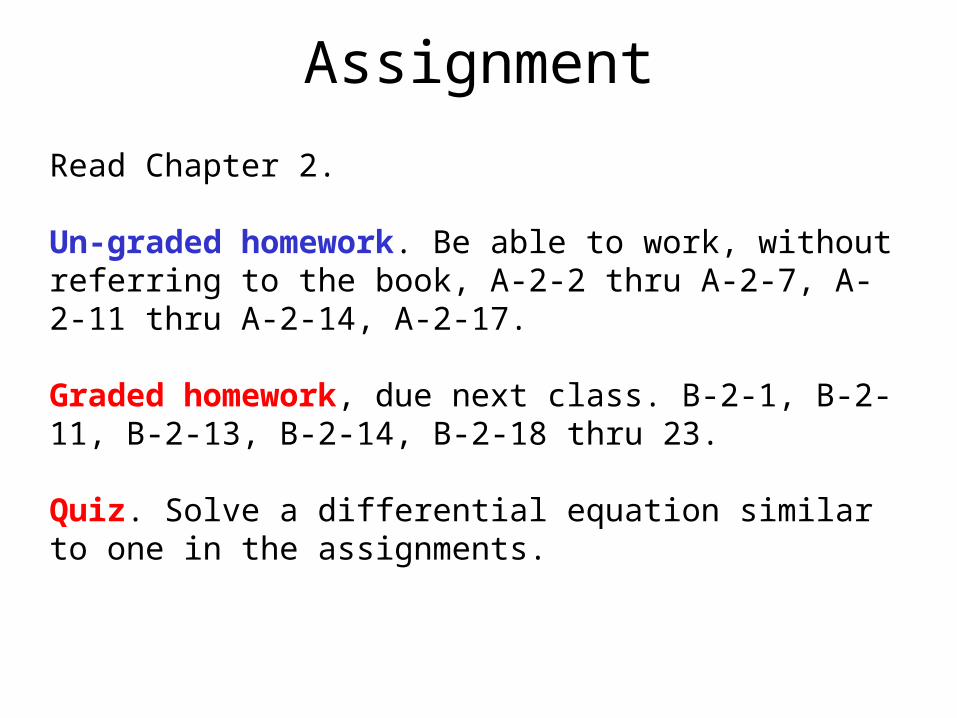
Assignment

Read Chapter 2.

Un-graded homework. Be able to work, without referring to the book, A-2-2 thru A-2-7, A-2-11 thru A-2-14, A-2-17.

Graded homework, due next class. B-2-1, B-2-11, B-2-13, B-2-14, B-2-18 thru 23.

Quiz. Solve a differential equation similar to one in the assignments.

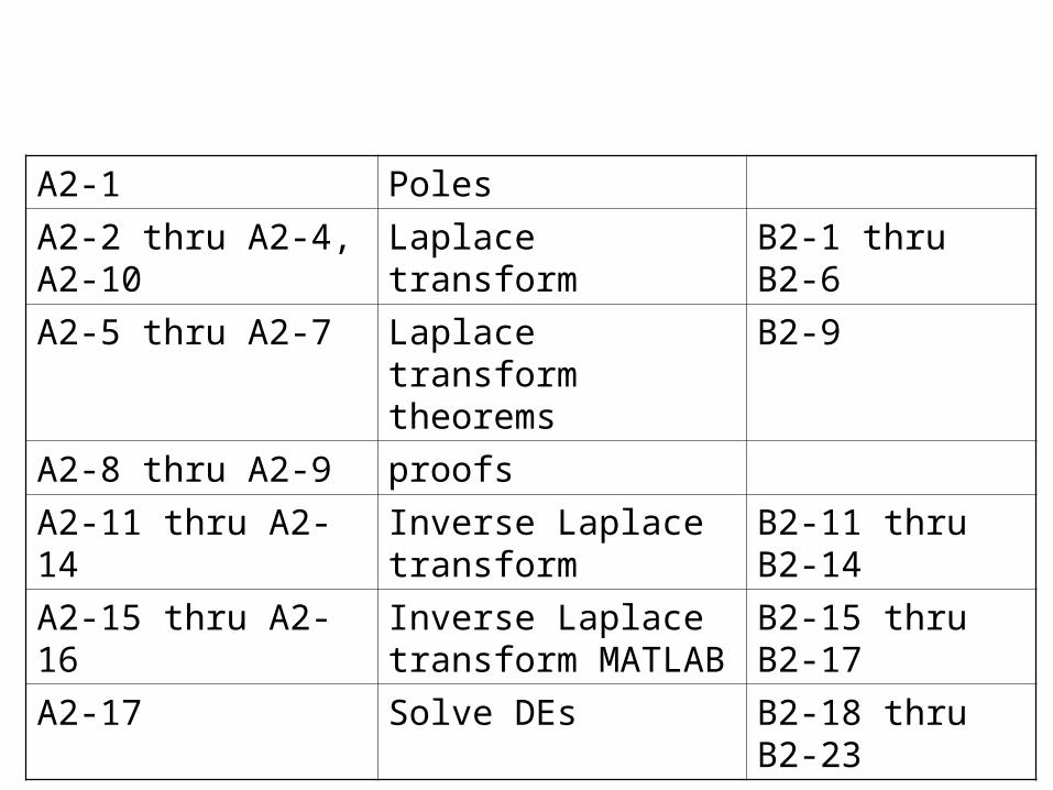
A2-1 Poles

A2-2 thru A2-4, A2-10 Laplace transform B2-1 thru B2-6

A2-5 thru A2-7 Laplace transform theorems

B2-9

A2-8 thru A2-9 proofs

A2-11 thru A2-14 Inverse Laplace transform

B2-11 thru B2-14

A2-15 thru A2-16 Inverse Laplace transform MATLAB

B2-15 thru B2-17

A2-17 Solve DEs B2-18 thru B2-23