the$3rd$acamworkshop,$june.$569,$2017 ......
TRANSCRIPT

S. Hayashida1, M. Kajino2, M. Deushi2, T. Sekiyama2, and X. Liu3
1. Faculty of Science, Nara Women’s University, Nara, Japan 2. Meteorological Research InsLtute, Tsukuba, Japan
3. Harvard-‐Smithsonian Center for Astrophysics, Cambridge, MassachuseQs, USA
The 3rd ACAM workshop, June. 5-‐9, 2017
Enhancement of the lower tropospheric ozone over China: Comparison of Ozone Monitoring Instrument (OMI) and
model simula>ons

IntroducLon • Satellite measurements have the advantage of making
observaLons over wide areas. • Almost 90 % of O3 is in the stratosphere, 10 % in the
troposphere: the amount of O3 in the boundary layer is usually only a small percentage of the total amount.
• Ozone profiling is a big challenge of satellite missions. • From OMI (Ozone Monitoring Instrument ) UV spectra, O3
profiles have been derived (Liu et al., ACP, 2010) • The lower tropospheric O3 distribuLon maps were
obtained from the OMI UV measurements (Hayashida et al., ACP, 2015).

Satellite data: OMI O3 profile
3
Liu et al., ACP, 2010: Xiong Liu and Kelly Chance successfully retrieved ozone profiles for 24 layers from OMI spectra, in 270-‐330 nm (270-‐309 nm in UV1, 312-‐330 nm in UV2), with 3-‐7 layers in the troposphere. • OpLmal esLmaLon with climatology by McPeters et al.
(2007) for a priori • 24th : 0 ~ 3 km, 23rd : 3~5 (or 6) km, 22nd : 5 ~ 8 (or 9) km • Horizontal resoluLon of 13 km× 48 km (nadir posiLon)
O3
O3 O3
O3
O3 O3
O3
O3 O3
O3
22
24
23
1 60 km
Level 3: archived 1 x 1 deg. Pre-‐ screening
Cloud fracLon < 0.2 RMS (UV2) < 2.4
Our Analysis
• S. Hayashida, X. Liu, et al.: ObservaIon of ozone enhancement in the lower troposphere over East Asia from a space-‐borne ultraviolet spectrometer, Atmos. Chem. Phys., 15, 9865–9881, 2015
OMI ozone profiles • In Hayashida et al., ACP, 2015: • we compared the OMI-‐derived O3 profiles over Beijing with airborne measurements (MOZAIC) and demonstrated the reliability of OMI O3 retrievals in the lower troposphere under enhanced ozone condiLons.
• we showed significant enhancement of O3 in the lower troposphere observed by OMI over central and eastern China (CEC) with Shandong as its center.
• The O3 enhancement is most notable in June every year.
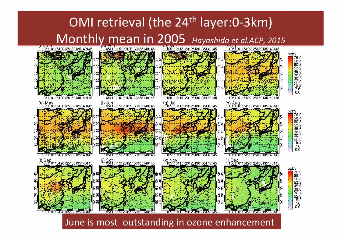
OMI retrieval (the 24th layer:0-‐3km) Monthly mean in 2005 Hayashida et al.ACP, 2015
June is most outstanding in ozone enhancement

UT/LS screening for 24th layer ozone Hayashida et al. Springer, in press
• However, O3 variability in the upper-‐troposphere/lower-‐stratosphere (UT/LS) region may lead a significant arLficial effect on lower tropospheric O3 due to large smoothing errors.
• Hayashida et al. (Springer, 2017) clarified the concept of screening out the arLficial effect and developed a UT/LS screening scheme.
• They were able to find a clear enhancement in lower tropospheric O3 over CEC in June 2006 even aler the UT/LS screening, and confirmed the conclusion described in Hayashida et al. (2015).
• In this study, we applied the screening for all OMI retrievals during the period from October, 2004 through December, 2013 to remove any suspect data that might be affected by the UT/LS ozone variability.

Grid SelecLon: Remove the grids in which the effect of the UT/LS O3 variability
on the 24th-‐layer O3 is larger than the threshold
“Douboul grids” were determined based on a model simulaLon, and those grids were removed from OMI dataset before analysis.
Hayashida et al., 2017, Springer, in press
“Study of lower tropospheric ozone over central and eastern China: Comparison of satellite observaIon with model simulaIon” was accepted to Land-‐Atmospheric InteracIons in Asia, Springer (to be published soon).
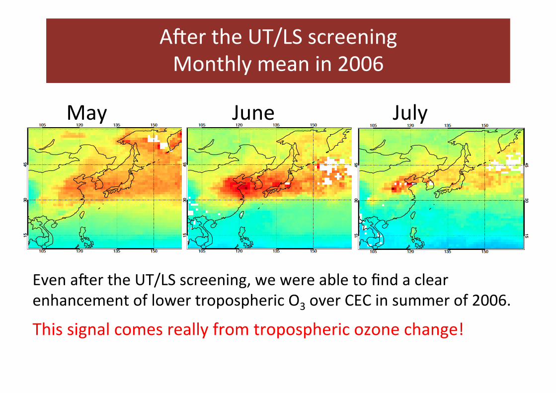
Aler the UT/LS screening Monthly mean in 2006
Even aler the UT/LS screening, we were able to find a clear enhancement of lower tropospheric O3 over CEC in summer of 2006.
May June July
This signal comes really from tropospheric ozone change!

A D
B C
Map of the 24th layer O3 in June 2005
Gray: a priori Blue: O3 retrieval Red: screened out (not used in analysis)
AIn summer: significant enhancement of O3 (larger than a priori)
B
We focus on ΔO3 = O3[retrieval] – O3[a priori] to track O3 enhancement.

A D
B C
Time series of ΔO3
Clear seasonal variaLon
Clear seasonal variaLon No seasonality
NegaLve in August

Cluster analysis of the >me series of ΔO3 the complete linkage method for hierarchical clustering
ΔO3
Month
Grids with similar seasonal variaLon were grouped into the same “cluster”.
Distance of two Datasets
N = 4 N=6

Time series of the monthly mean values of the ΔO3 at 24th layer in the four clusters 1-‐4

Time series of the monthly mean values of the ΔO3 at 24th layer in the clusters 4-‐1, 4-‐2-‐1, 4-‐2-‐2 (N=6)

Annual anthropogenic NO2 emission in 2006 [µgNO2/m2/s] (MaCCity)
The high NO2 emission area very clearly corresponds to the areas of Clusters 1 and 2 as shown with a thick line.
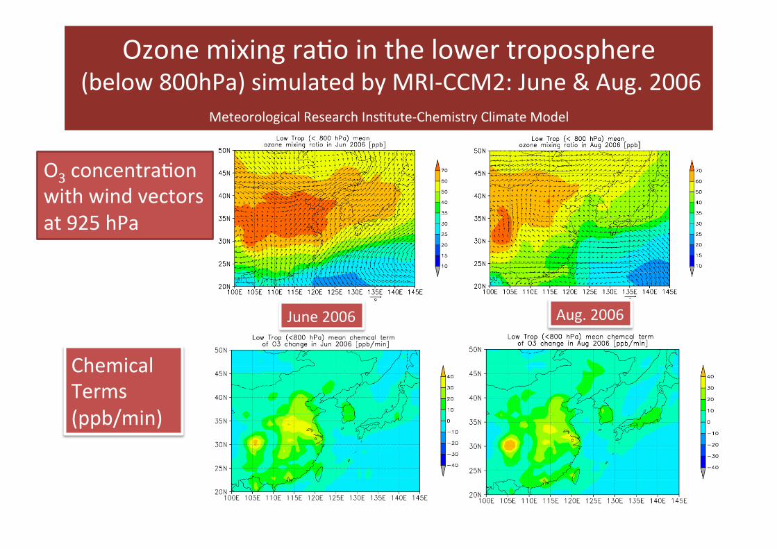
Ozone mixing raLo in the lower troposphere (below 800hPa) simulated by MRI-‐CCM2: June & Aug. 2006
Meteorological Research InsLtute-‐Chemistry Climate Model
Chemical Terms (ppb/min)
O3 concentraLon with wind vectors at 925 hPa
June 2006 Aug. 2006

• The OMI O3 profile products (by Liu et al.. 2010) over China – We focused on the O3 anomaly, which is defined as – ΔO3 = O3[retrieval] – O3[a priori] – This analysis is effecLve in tracking O3 enhancement under polluted
condiLons, because our focus is the temporally high O3 compared to background levels.
• Cluster analysis to the ΔO3 data at the 24th layer – Over the North China Plain and Sichuan basin, O3 has outstanding
seasonality with high values in summer (June, in parLcular) and low values in winter.
– These anomalous O3 value areas correspond to areas that is known as high NO2 emissions.
• Comparison with ACTM simulaLons – Cluster 1 corresponds to areas of high chemical producLon rates in June. – Along the coastal area in August, O3 tends to drop to negaLve values, which
can be interpreted as due to the inland inflow of clean oceanic air.
Summary