theoretical chemistry university of nijmegen the netherlandspwormer/teachmat/matlab_dictaat.pdf ·...
TRANSCRIPT
Matlab for Chemists
P.E.S. Wormer
Theoretical Chemistry
University of Nijmegen
The Netherlands
April 2003

ii
PREFACE
matlab is an interactive program package for numerical computation andvisualization. It originated in the middle of the 1980s as a user interfaceto matrix manipulation packages written in fortran. Hence its name:“Matrix Laboratory”. Over the years the system has been extended, it nowincludes a programming language, extensive visualization tools, and manynumerical methods.
These are notes accompanying a course in matlab for chemistry andnatural science students at the University of Nijmegen. The course has thefollowing objectives:
• Offering of practical exercises supporting an obligatory course in linearalgebra.
• Offering of practical exercises supporting an obligatory course in quan-tum mechanics.
• A first introduction to programming (loops, if then else constructs,functions).
• A tool for fitting and plotting data obtained in the chemical laboratory.
Although no new mathematical concepts are introduced in the present lec-tures, the mathematical knowledge necessary to do the matlab exercises,is briefly reviewed.
The author thanks dr. B. J. W. Polman of the Subfaculty of Mathematicsfor his careful reading of the notes and his useful comments.
Contents
Preface . . . . . . . . . . . . . . . . . . . . . . . . . . . . . . . . . ii
1 Vectors and their operations 1
1.1 Scalars and vectors . . . . . . . . . . . . . . . . . . . . . . . . 1
1.2 Linear independent and orthogonal vectors . . . . . . . . . . 7
1.3 Exercises . . . . . . . . . . . . . . . . . . . . . . . . . . . . . 9
2 Matrices 13
2.1 Matrix multiplication . . . . . . . . . . . . . . . . . . . . . . . 13
2.2 Non-singular and special matrices . . . . . . . . . . . . . . . . 15
2.3 Matrix factorizations . . . . . . . . . . . . . . . . . . . . . . . 18
2.4 Exercises . . . . . . . . . . . . . . . . . . . . . . . . . . . . . 19
3 Scripts and plotting 23
3.1 Scripts . . . . . . . . . . . . . . . . . . . . . . . . . . . . . . . 23
3.2 Plotting . . . . . . . . . . . . . . . . . . . . . . . . . . . . . . 24
3.3 Exercises . . . . . . . . . . . . . . . . . . . . . . . . . . . . . 26
4 Matrices continued, flow control 27
4.1 Matrix sections . . . . . . . . . . . . . . . . . . . . . . . . . . 27
4.2 Flow control . . . . . . . . . . . . . . . . . . . . . . . . . . . . 29
4.3 Exercises . . . . . . . . . . . . . . . . . . . . . . . . . . . . . 32
5 Least squares fitting 37
5.1 Linear equations . . . . . . . . . . . . . . . . . . . . . . . . . 37
5.2 Least squares . . . . . . . . . . . . . . . . . . . . . . . . . . . 38
5.3 Necessity of least squares . . . . . . . . . . . . . . . . . . . . 42
5.4 Exercises . . . . . . . . . . . . . . . . . . . . . . . . . . . . . 44
6 Functions and function functions 47
6.1 Functions . . . . . . . . . . . . . . . . . . . . . . . . . . . . . 47
6.2 Function functions . . . . . . . . . . . . . . . . . . . . . . . . 49
6.3 Coupled first order differential equations . . . . . . . . . . . . 51
6.4 Higher order differential equations . . . . . . . . . . . . . . . 54
6.5 Exercises . . . . . . . . . . . . . . . . . . . . . . . . . . . . . 55
iii
iv CONTENTS
7 More plotting 59
7.1 3D plots . . . . . . . . . . . . . . . . . . . . . . . . . . . . . . 597.2 Handle Graphics . . . . . . . . . . . . . . . . . . . . . . . . . 617.3 Handles of graphical objects . . . . . . . . . . . . . . . . . . . 617.4 Polar plots . . . . . . . . . . . . . . . . . . . . . . . . . . . . 657.5 Exercises . . . . . . . . . . . . . . . . . . . . . . . . . . . . . 66
8 Cell arrays and structures 69
8.1 Cell arrays . . . . . . . . . . . . . . . . . . . . . . . . . . . . . 698.2 Characters . . . . . . . . . . . . . . . . . . . . . . . . . . . . . 748.3 Structures . . . . . . . . . . . . . . . . . . . . . . . . . . . . . 768.4 Exercises . . . . . . . . . . . . . . . . . . . . . . . . . . . . . 80

1. Vectors and their operations
1.1 Scalars and vectors
Variables, assignments, scalars, row and column vectors, echoing of input,
transposition, length versus norm of vector, inner products. Difference be-
tween vector- and dot- operations.
All internal operations in matlab are performed with floating point num-
bers 16 digits long, as e.g., 3.141592653589793 or 0.3141592653589793e-1
(e-1 indicates 10−1). The simplest data structure in matlab is the scalar
(handled by matlab as a 1 × 1 matrix). Scalars can be given names and
assigned values, e.g.,
>> num_students = 25;
>> Temperature = 272.1;
>> Planck = 6.6260755e-34;
It is important to understand fully the difference between the mathematical
equality a = b (which can be written equally well as b = a) and the matlab
assignment a=b. In the latter statement it is necessary that the right hand
side has a value at the time that the statement is executed. The right hand
side is first fully evaluated and then the result is assigned to the left hand
side. Example:
>> a = 33.33;
>> a = 3*a - a
a =
66.6600
First the expression 3*a-a is fully evaluated. The value of a, which it has
just before the statement, is substituted everywhere. Only at the end of the
evaluation a is assigned a new value by means of the assignment symbol =.
A variable name must start with a lower- or uppercase letter and only the
first 31 characters of the name are used by matlab. Digits, letters and un-
derscores are the only allowed characters in the name of a variable. matlab
is case sensitive: the variable temperature is another than Temperature.
Scalars can be added: a+b, subtracted: a-b, multiplied: a*b, divided: a/b
and taken to a power: a^b. The usual priority rules hold (multiplication
1

2 CHAPTER 1. VECTORS AND THEIR OPERATIONS
before addition, etc.), but it is better not to rely on this and to force the pri-
ority by brackets. Do not write a/b^3, but (a/b)^3, or a/(b^3), whatever
your intention is.
The second simplest data structure in matlab is the vector, which is
simply a sequence of floating point numbers. Vectors come in two flavors:
row vectors and column vectors. Row vectors are entered either space de-
limited or comma delimited, as
>> a=[1 2 3 -2 -4]
a =
1 2 3 -2 -4
>> b=[1,2,3,-2,-4]
b =
1 2 3 -2 -4
The sequence is delimited by square brackets. Notice that the vectors a and
b are indeed equal. After they have been entered at the matlab prompt
(>>), matlab echoes the input. This echoing of input is suppressed when
the statement is ended by a semicolon (;). The vector is shown by typing
its name, thus,
>> a=[1 2 3 -2 -4]; % No output
>> a % echo the vector a
a =
1 2 3 -2 -4
Note that comments may be entered preceded by a % sign, they run until
end of line. The rules for naming vectors are the same as for scalars. (Case
sensitive, starting with letters, length ≤ 31, only digits, letters and under-
scores in the name). Column vectors are entered either semicolon delimited
or end of line delimited.
>> a=[1;2;3]
a =
1
2
3
>> a=[
1
2
3]

1.1. SCALARS AND VECTORS 3
a =
1
2
3
A row vector can be turned into a column vector and vice versa (transposi-
tion) by the transposition operator (’)
>> a=[1 2 3];
>> b=a’
b =
1
2
3
>> c=b’
c =
1 2 3
Note
Experience shows that the most common error in matlab is forgetting
whether a vector is a row or a column vector. We adhere strictly to the
convention that a vector is a column.
The easiest way to enter a column vector is as a row plus immediate
transposition, thus,
>> a=[5 4 3 2]’
a =
5
4
3
2
A single element of a row or column vector can be retrieved as e.g., a(4),
this gives the fourth element of a (the number 2 in the example). A range
can be returned by the use of a colon (:). For instance, b=a(2:3) returns
a column vector b with the digits 4 and 3 as elements. The word end gives
the end of a vector: b=a(2:end) creates a column vector b containing 4, 3,
2.
In mathematics and physics the norm and the length of a vector are often
used as synonyms. In matlab the two concepts are different, length(a)
returns the number of components of a (the dimension of the vector), while
norm(a) returns the norm of a. Remember that the norm |a| of a is by
definition |a| = √a · a.
4 CHAPTER 1. VECTORS AND THEIR OPERATIONS
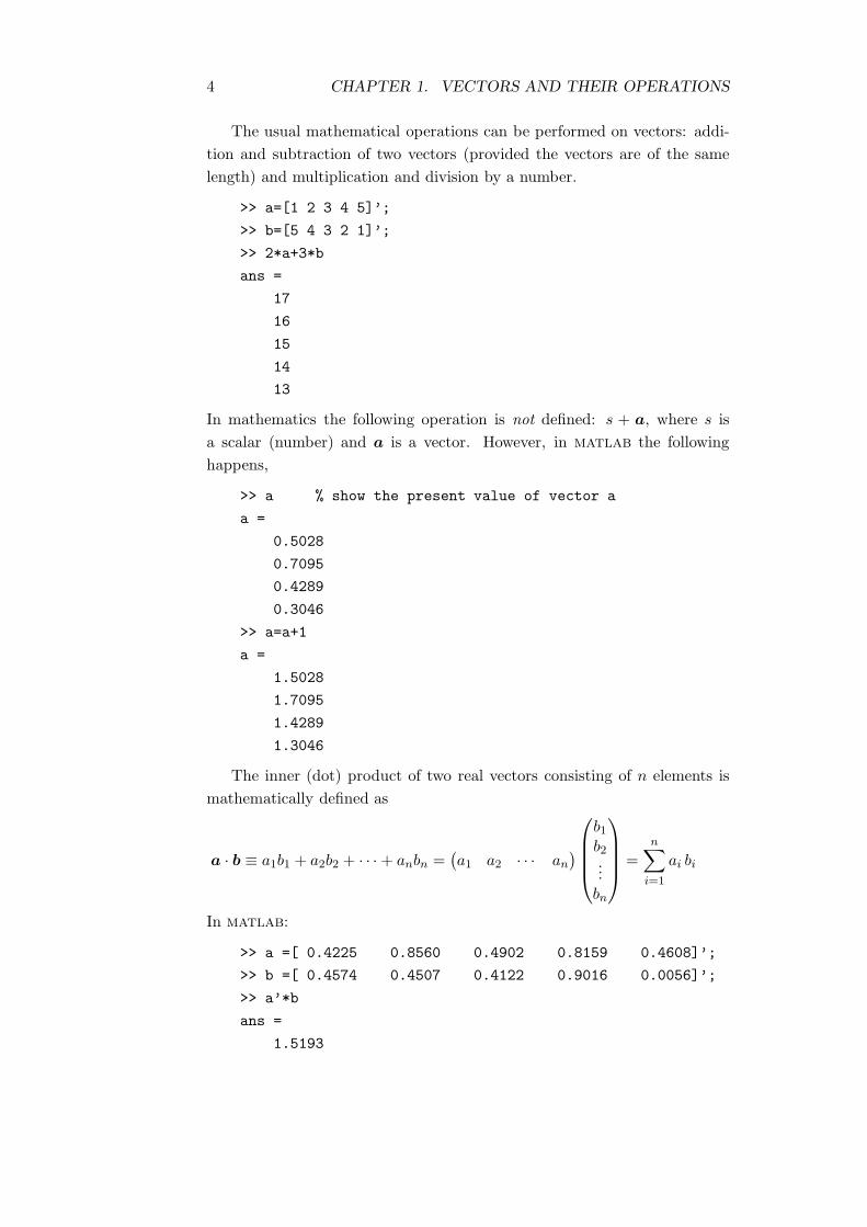
The usual mathematical operations can be performed on vectors: addi-
tion and subtraction of two vectors (provided the vectors are of the same
length) and multiplication and division by a number.
>> a=[1 2 3 4 5]’;
>> b=[5 4 3 2 1]’;
>> 2*a+3*b
ans =
17
16
15
14
13
In mathematics the following operation is not defined: s + a, where s is
a scalar (number) and a is a vector. However, in matlab the following
happens,
>> a % show the present value of vector a
a =
0.5028
0.7095
0.4289
0.3046
>> a=a+1
a =
1.5028
1.7095
1.4289
1.3046
The inner (dot) product of two real vectors consisting of n elements is
mathematically defined as
a · b ≡ a1b1 + a2b2 + · · ·+ anbn =(a1 a2 · · · an
)
b1b2...bn
=
n∑
i=1
ai bi
In matlab:
>> a =[ 0.4225 0.8560 0.4902 0.8159 0.4608]’;
>> b =[ 0.4574 0.4507 0.4122 0.9016 0.0056]’;
>> a’*b
ans =
1.5193

1.1. SCALARS AND VECTORS 5
Recalling the definition of the norm of a vector, we see that sqrt(a’*a)
gives the very same answer as norm(a). Both sqrt and norm are functions
known to matlab.
Recall that the set of all column vectors with n real components forms a
vector space commonly denoted by Rn. The geometric meaning of the inner
product in Rn is well-known in R
3. It is the following: it gives the angle
between two vectors,
r1 · r2 = r1 r2 cosφ.
Here ri ≡ |ri| ≡√ri · ri is the norm of vector ri (i = 1, 2) and φ is the angle
between the two vectors. We give an example of the computation of φ:
>> % Introduce two column vectors for the example:
>> a=[23 0 -21]’;
>> b=[0 10 0]’;
>> % Compute their lengths:
>> la = norm(a);
>> lb = norm(b);
>> % Now the cosine of the angle
>> cangle = (a’*b)/(la*lb);
>> % the angle itself
>> phi = acos(cangle)
phi =
1.5708
>> % Radians, convert to degrees:
>> phi*180/pi
ans =
90
Explanation:
Division of two numbers is by the slash (/). matlab knows the inverse
cosine (acos), which gives results in radians. matlab knows π = 3.14 . . .,
it is simply the variable pi. Do not use the name pi for anything else!
matlab has lots of elementary mathematical functions that all work ele-
mentwise on vectors and matrices. In Table 1.1 we show the most important
mathematical functions.
We end this section, by introducing the dot operations, which are not
defined as such in linear algebra. It often happens that one wants to divide
all the individual elements of vectors. Suppose we have measured 5 numbers
as a function of a certain quantity and that we also made a fit of the measured
values. To compute the percentage error of the fit we proceed as follows:

6 CHAPTER 1. VECTORS AND THEIR OPERATIONS
Table 1.1: Elementary mathematical functions. All operate on the elements
of matrices.
abs Absolute value and complex magnitudeacos, acosh Inverse cosine and inverse hyperbolic cosineacot, acoth Inverse cotangent and inverse hyperbolic cotangentacsc, acsch Inverse cosecant and inverse hyperbolic cosecantangle Phase angleasec, asech Inverse secant and inverse hyperbolic secantasin, asinh Inverse sine and inverse hyperbolic sineatan, atanh Inverse tangent and inverse hyperbolic tangentatan2 Four-quadrant inverse tangentceil Round toward infinitycomplex Construct complex data from real and
imaginary componentsconj Complex conjugatecos, cosh Cosine and hyperbolic cosinecot, coth Cotangent and hyperbolic cotangentcsc, csch Cosecant and hyperbolic cosecantexp Exponentialfix Round towards zerofloor Round towards minus infinitygcd Greatest common divisorimag Imaginary part of a complex numberlcm Least common multiplelog Natural logarithmlog2 Base 2 logarithm and dissect floating-point numbers
into exponent and mantissalog10 Common (base 10) logarithmmod Modulus (signed remainder after division)nchoosek Binomial coefficient or all combinationsreal Real part of complex numberrem Remainder after divisionround Round to nearest integersec, sech Secant and hyperbolic secantsign Signum functionsin, sinh Sine and hyperbolic sinesqrt Square roottan, tanh Tangent and hyperbolic tangent

1.2. LINEAR INDEPENDENT AND ORTHOGONAL VECTORS 7
>> % Enter the observed values:
>> obs = [ -0.3012 -0.0999 0.0527 0.1252 0.2334]’;
>> % Enter the fitted values:
>> fit = [ -0.3100 -0.1009 0.0531 0.1263 0.2479]’;
>> % Percentage error: (put result into vector error
>> % and transpose for typographical reasons)
>> error=[100*(obs-fit)./obs]’
error =
-2.9216 -1.0010 -0.7590 -0.8786 -6.2125
Note the operation ./, this is pointwise division, i.e., it computes
error(i) = 100 ∗ (obs(i)− fit(i))/obs(i) for i = 1, . . . , 5,
successively. Suppose we forgot the dot in the division, then matlab does
not give an error, but the following unexpected result1 (a 5× 5 matrix):
>> error=[100*(obs-fit)/obs]’
error =
-2.9216 -0.3320 0.1328 0.3652 4.8141
0 0 0 0 0
0 0 0 0 0
0 0 0 0 0
0 0 0 0 0
Also pointwise multiplication is possible, example:
>> [1 2 3 4]’.*[24 12 8 6]’
ans =
24
24
24
24
1.2 Linear independent and orthogonal vectors
Linear dependence, orthogonality
Returning to linear algebra, we recall the following two definitions:
1The reason is that if matlab meets an expression of the type s/a, where a is a columnvector, it tries to solve the equation x ·a = s, and obviously one of the possible solutions isthe row vector x = (s/a1, 0, 0, . . . , 0). We do not get a matrix of five of these row vectors,because there is a prime on the result, but the transposed matrix.

8 CHAPTER 1. VECTORS AND THEIR OPERATIONS
1. The set of n non-null vectors r1, r2, . . . , rn is linearly dependent if an
arbitrary member can be written as a linear combination of the others,
i.e., if expansion coefficients cj can be found so that the following is
true for any i
ri = c1r1 + · · · ci−1ri−1 + ci+1ri+1 + · · · cnrn,
where ri does not appear on the right hand side. If a set of vec-
tors is not linearly dependent it is (not surprisingly) called linearly
independent.
2. Two vectors ri = (r1i r2i · · · rni) and rj = (r1j r2j · · · rnj) are
orthogonal if
ri · rj ≡ r1i r1j + r2i r2j + · · · + rni rnj = 0.
Remember further that orthogonal vectors are linearly independent.
A basis of Rn is a maximum set of linearly independent real vectors of
dimension n. A set of vectors ri forms an orthogonal basis of Rn if
ri · rj = 0 for i, j = 1, . . . , n.
This is usually compactly written as follows
ri · rj = r2i δij with δi,j =
1 if i = j
0 if i 6= jand r2i ≡ ri · ri. (1.1)
An arbitrary real vector a of dimension n can be written as a linear combi-
nation of the n orthogonal vectors ri
a = a1r1 + a2r2 + · · ·+ anrn =
n∑
i=1
ai ri,
because this is a maximum set of linearly independent vectors in Rn. It is
easy to compute the expansion coefficients ai:
rj · a =
n∑
i=1
ai rj · ri =n∑
i=1
ai r2i δi,j = aj r
2j ,
so that aj = rj · a/r2j for all j = 1, . . . , n.
As a geometric application we remember that we learned in our linear
algebra course about a plane in the space R3. Consider a certain fixed vector
x with norm x. All vectors r orthogonal to x form a plane, i.e., all vectors
r in the plane satisfy r · x = 0. An orthogonal basis of the plane can be
constructed as follows.

1.3. EXERCISES 9
1. Choose a vector y′ that is not a multiple of x, x and y′ are linearly
independent.
2. Orthogonalize y′ onto x by the following equation,
y = y′ − x(x · y′)/x2.
We check the orthogonality:
x · y = x · y′ − (x · x)(x · y′)/x2 = x · y′ − x · y′ = 0,
since x2 = x · x. Hence y (with norm y) is in the plane orthogonal to
x.
3. To obtain the second basis vector of the plane we can choose a third
vector which is linearly independent of x and y and orthogonalize. Or,
we can form the vector product z = x × y, which is less general as
it only works in R3, but is easier. [The cross product in matlab is
r3=cross(r1,r2)].
The vectors x, y and z form a right-handed orthogonal frame (set of axes)
of R3. An arbitrary vector a in this space can be decomposed as follows
a = x(x · a)/x2 + y(y · a)/y2 + z(z · a)/z2.
If we want to reflect a in the y-z plane (which is orthogonal to the given
vector x), we simply keep the y and z components of a unchanged and
change the sign of its component vector along x.
1.3 Exercises
Exercise 1.
Try to reproduce the examples above to get acquainted with matlab.
Exercise 2.
Type in the column vector a containing the six subsequent elements: 1, −2,
3, −4, 5, −6. Normalize this vector. That is, determine its norm and divide
the vector by it. Check your result by computing the norm of the normalized
vector.
Exercise 3.
Type in the column vector b containing the subsequent elements: −1, 2, −3,
4, −5, 6. Determine the angle (in degrees) of this vector with the vector of
the previous exercise. The answer is very simple, explain why.

10 CHAPTER 1. VECTORS AND THEIR OPERATIONS
Exercise 4.
A root (or zero) of a polynomial P (x) = a0 + a1x+ · · ·+ anxn is a solution
of the equation P (x) = 0. The main theorem of algebra states that this
equation has exactly n roots, which may be complex.
Determine the roots of the 4th degree polynomial
x4 − 11.0x3 + 42.35x2 − 66.550x + 35.1384.
Hint:
Put the coefficients of powers of x into a column array c (in decreasing
power of x) and issue the command roots(c) (a call to the matlab function
roots).
Exercise 5.
In the USA the curious temperature scale Fahrenheit2 is in daily use.
To convert to the Celsius scale use the formula C = 5(F - 32)/9. Prepare
a table F starting at −20 C, ending at 100 C with steps of 5 C that
contains Celsius converted to Fahrenheit.
Hint: A row vector containing the Celsius steps can be prepared by the
command: C=[-20:5:100]. To get a nice table on the screen use [C’ F’].
Compute in degrees Celsius the points: 0, 32, 96, and 212 F by interpo-
lation with the matlab function interp1. For instance, interp1(F,C,104)
returns 40.
Exercise 6.
Consider the methane molecule CH4. The four protons are on the 4 al-
ternating corners of a cube, with one CH bond pointing into the (1, 1, 1)
direction and the other bonds pointing to other corners in agreement with
methane being tetrahedral. All C–H bondlengths are 1.086 A. Compute the
6 H–C–H angles and the 6 H–H distances (all should be equal due to the
high symmetry of methane).
Exercise 7.
Compute
[1 2 3 4]’.*[24 12 8 6]’
[1 2 3 4]’*[24 12 8 6]
[1 2 3 4]*[24 12 8 6]’
2It is named after Gabriel Daniel Fahrenheit (1686–1736), who invented it in 1714,while working in Amsterdam.

1.3. EXERCISES 11
Explain the differences.
Exercise 8.
Let x = (−2,−1, 3, 4). Compute4∑
i=1
x5i .
Hint:
The matlab function sum(y) sums the components of the vector y.
Exercise 9.
Consider the vector x =
213
. Construct two vectors y and z orthogonal
to x and to each other. Compute the components of a =
3−12
along x,
y and z. Then reflect the vector a into the plane spanned by y and z. Let
the reflected vector be a′. Verify that a− a′ is orthogonal to the reflection
plane.
Exercise 10.
The vectors
r1 =
321
and r2 =
2−1−4
are orthogonal. We easily get an orthogonal basis for R3 by defining r3 =
r1 × r2. Calculate the components of
e1 =
100
and e2 =
010
and e3 =
001
with respect to the basis r1, r2, r3.
Exercise 11.
The O–H bond distance in the water molecule H2O is 0.91 A. The H-O-H
angle is 104.69. Compute the distance between the protons.
Hint: Compute the Cartesian coordinates of the vectors x1 =−−→OH1 and
x2 =−−→OH2 with respect to an orthonormal (= orthogonal with normalized
basis vectors) frame centered at O. The distance between H1 and H2 is
|x1 − x2|.

12 CHAPTER 1. VECTORS AND THEIR OPERATIONS

2. Matrices
Before introducing matrix multiplication we wish to point out that—as a
modern computer package—matlab has extensive built-in documentation.
The command helpdesk gives access to a very elaborate interactive help
facility. The command help cmd gives help on the specified command cmd.
The command more on causes help to pause between screenfuls if the help
text runs to several screens. In the online help, keywords are capitalized to
make them stand out. Always type commands in lowercase since all com-
mand and function names are actually in lowercase. Recall in this context
that matlab is case sensitive. Don’t be confused by the capitals in the help.
2.1 Matrix multiplication
Matrices and their multiplication.
Turning to matrices, we first observe that a column vector of length n is a
special case of an n ×m matrix, namely one with m = 1. A matrix can be
constructed by concatenation. This is the process of joining smaller matrices
(or vectors) to make bigger ones. In fact, you made your first matrix by
concatenating its individual elements. The pair of square brackets, [], is
the concatenation operator. Example:
>> a = [1 3 -5]’;
>> b = [2 1 7]’;
>> c = [-1 6 1]’;
>> [a b c]
ans =
1 2 -1
3 1 6
-5 7 1
>> [a b c c b a]
ans =
1 2 -1 -1 2 1
3 1 6 6 1 3
-5 7 1 1 7 -5
Amatrix may be entered as rows, just like column vectors, which for matlab
are in fact nothing but non-square matrices. Example of entering a 2 × 4
matrix (2 rows, 4 columns):
13
14 CHAPTER 2. MATRICES
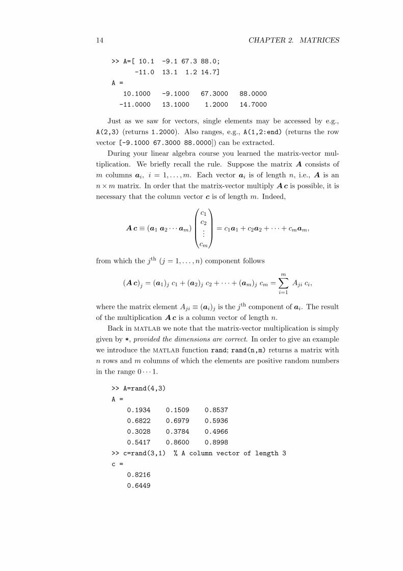
>> A=[ 10.1 -9.1 67.3 88.0;
-11.0 13.1 1.2 14.7]
A =
10.1000 -9.1000 67.3000 88.0000
-11.0000 13.1000 1.2000 14.7000
Just as we saw for vectors, single elements may be accessed by e.g.,
A(2,3) (returns 1.2000). Also ranges, e.g., A(1,2:end) (returns the row
vector [-9.1000 67.3000 88.0000]) can be extracted.
During your linear algebra course you learned the matrix-vector mul-
tiplication. We briefly recall the rule. Suppose the matrix A consists of
m columns ai, i = 1, . . . ,m. Each vector ai is of length n, i.e., A is an
n×m matrix. In order that the matrix-vector multiply Ac is possible, it is
necessary that the column vector c is of length m. Indeed,
Ac ≡ (a1 a2 · · ·am)
c1c2...cm
= c1a1 + c2a2 + · · ·+ cmam,
from which the jth (j = 1, . . . , n) component follows
(Ac)j = (a1)j c1 + (a2)j c2 + · · ·+ (am)j cm =m∑
i=1
Aji ci,
where the matrix element Aji ≡ (ai)j is the jth component of ai. The result
of the multiplication Ac is a column vector of length n.
Back in matlab we note that the matrix-vector multiplication is simply
given by *, provided the dimensions are correct. In order to give an example
we introduce the matlab function rand; rand(n,m) returns a matrix with
n rows and m columns of which the elements are positive random numbers
in the range 0 · · · 1.
>> A=rand(4,3)
A =
0.1934 0.1509 0.8537
0.6822 0.6979 0.5936
0.3028 0.3784 0.4966
0.5417 0.8600 0.8998
>> c=rand(3,1) % A column vector of length 3
c =
0.8216
0.6449

2.2. NON-SINGULAR AND SPECIAL MATRICES 15
0.8180
>> A*c % Matrix-vector multiply
ans = % A column vector of length 4
0.9545
1.4961
0.8989
1.7357
>> d=rand(4,1) % A column vector of length 4
d =
0.6602
0.3420
0.2897
0.3412
>> A*d % Try a matrix vector multiply
??? Error using ==> *
Inner matrix dimensions must agree.
Suppose now that we have a set of k column vectors c1, c2, . . . , ck, all of
lenght m. We can apply the matrix-vector multiplication rule to the vector
cj and do this consecutively for j = 1, . . . , k,
(Acj)j′ =
m∑
i=1
Aj′i (cj)i .
If we introduce an m× k matrix C with general element Cij ≡ (cj)i we can
write
(AC)j′j =
m∑
i=1
Aj′iCij
with j′ = 1, . . . , n and j = 1, . . . , k. The second (column) index of A must
agree with the first (row) index of C, otherwise matrix multiplication is not
possible. matlab refers to these indices as ‘inner matrix dimensions’. In this
parlance n and k are the ‘outer matrix dimensions’, they are independent.
2.2 Non-singular and special matrices
Non-singular matrices and determinant. The unit matrix, random matrix and
a matrix with ones.
The identity (or unit) matrix I plays an important role in linear algebra. It
is a square matrix with off-diagonal elements zero and the number one on
the diagonal,
(I)ij = δij ,
where the Kronecker delta was defined in Eq. (1.1). matlab has the pho-
netic name ‘eye’ for the function that returns the identity matrix.

16 CHAPTER 2. MATRICES
>> eye(4)
ans =
1 0 0 0
0 1 0 0
0 0 1 0
0 0 0 1
The command ones(n) returns an n × n matrix containing unity in all
entries. In Table 2.1 we list a few more of these commands.
Table 2.1: Elementary matrices
blkdiag Construct a block diagonal matrix from input argumentseye Identity matrixlinspace Generate linearly spaced vectorslogspace Generate logarithmically spaced vectorsones Create an array of all onesrand Uniformly distributed random numbers and arraysrandn Normally distributed random numbers and arrayszeros Create an array of all zeros
The following facts are proved in linear algebra.
1. An n × n matrix A is called non-singular if it has an inverse. That
is, another n × n matrix A−1 (the inverse of A) exists that has the
property A−1A = AA−1 = I.
2. If the n columns of an n×n matrix are linearly independent then the
matrix is non-singular.
3. If the n rows of an n × n matrix are linearly independent then the
matrix is non-singular.
4. If a square matrix is non-singular then its columns are linearly inde-
pendent and so are its rows.
5. Remember that the determinant det(A) of the real square matrix A
is a (fairly complicated) map A 7→ R, i.e., det(A) is a real number.
The square matrix A is non-singular if and only if det(A) 6= 0.
>> A=rand(4,4) % Make a square matrix
A =
0.5341 0.5681 0.4449 0.9568
0.7271 0.3704 0.6946 0.5226

2.2. NON-SINGULAR AND SPECIAL MATRICES 17
0.3093 0.7027 0.6213 0.8801
0.8385 0.5466 0.7948 0.1730
>> det(A) % What is its determinant?
ans =
0.0617 % Non-zero, the inverse of A exists.
>> Ai=inv(A) % Calculate the inverse
Ai =
3.6375 0.3718 0.0517 -3.0577
-3.2104 0.1104 -0.6997 3.7590
-1.9243 3.4861 0.0636 1.0540
0.3974 -2.4293 0.9644 0.0306
>> A*Ai-eye(4) % Subtract unit matrix
ans =
1.0e-015 * % Prefactor for the total matrix
-0.1110 -0.2220 0.0555 -0.0278
-0.0139 -0.2220 -0.0069 -0.0278
0 0 -0.1110 -0.0486
0.1943 -0.2220 0.1110 0
Here we used that matrices of the same dimensions can be subtracted and
we see that A A−1 is equal to the identity matrix within numerical precision
(15 to 16 digits). Here matlab applies the rule that cA gives a matrix in
which each individual matrix element is multiplied by the real number c.
We have seen that the operator ’ turns a row vector into a column
vector and vice versa. If we replace all rows of a matrix by its columns we
transpose the matrix, i.e., ifA has the matrix elements Aij , i = 1, . . . , n, j =
1, . . . ,m then AT has the matrix elements Aji, i = 1, . . . , n, j = 1, . . . ,m.
Transposition of matrices is performed by ’ as well.
>> A=rand(4,2)
A =
0.4235 0.2259
0.5155 0.5798
0.3340 0.7604
0.4329 0.5298
>> B=A’
B =

18 CHAPTER 2. MATRICES
0.4235 0.5155 0.3340 0.4329
0.2259 0.5798 0.7604 0.5298
2.3 Matrix factorizations
QR decomposition of arbitrary matrices and diagonalization of symmetric ma-
trices.
The purpose of this section is to introduce the important matlab functions
qr, eig, and sort. Before introducing these functions, we recall again some
relevant linear algebra.
A real n × n matrix Q = (q1, q2, . . . , qn) is called orthogonal when its
columns are orthonormal (orthogonal and normalized). This condition can
be expressed in two ways,
QTQ = I ⇐⇒ qi · qj = δij for i, j = 1, . . . , n. (2.1)
It follows immediately that also the rows of Q are orthonormal, because,
QTQ = I =⇒ QT = Q−1 =⇒ QQT = I
⇒ δij =(QQT
)
ij=
∑
k
QikQTkj =
∑
k
QikQjk. (2.2)
Since the sum is over the column index k, the rightmost expression is nothing
but the inner product between row i and row j of Q.
An important theorem of linear algebra states that any real n×m matrix
A can be factorized as
A = QR,
where Q is an n× n orthogonal matrix and R is an n×m upper triangular
matrix. (Remember that an upper triangular matrix R has only vanishing
elements below the main diagonal, i.e., Rij = 0 for i > j). This theorem
is known as the “QR decomposition” of A. One way of looking upon this
theorem is as a decomposition of the columns aj of A in an orthonormal
basis qk:
Aij =
n∑
k=1
QikRkj =
j∑
k=1
(qk)iRkj ⇐⇒ (aj)i =
j∑
k=1
(qk)iRkj
⇔ aj =
j∑
k=1
qkRkj = q1R1j + q2R2j + · · ·+ qjRjj. (2.3)
A matrix D is called diagonal when all its off-diagonal elements Dij , i 6=j, are zero, Dij = di δij . A real n × n matrix H is called symmetric if
H = HT , i.e., Hij = Hji for all i, j = 1, . . . , n.
2.4. EXERCISES 19
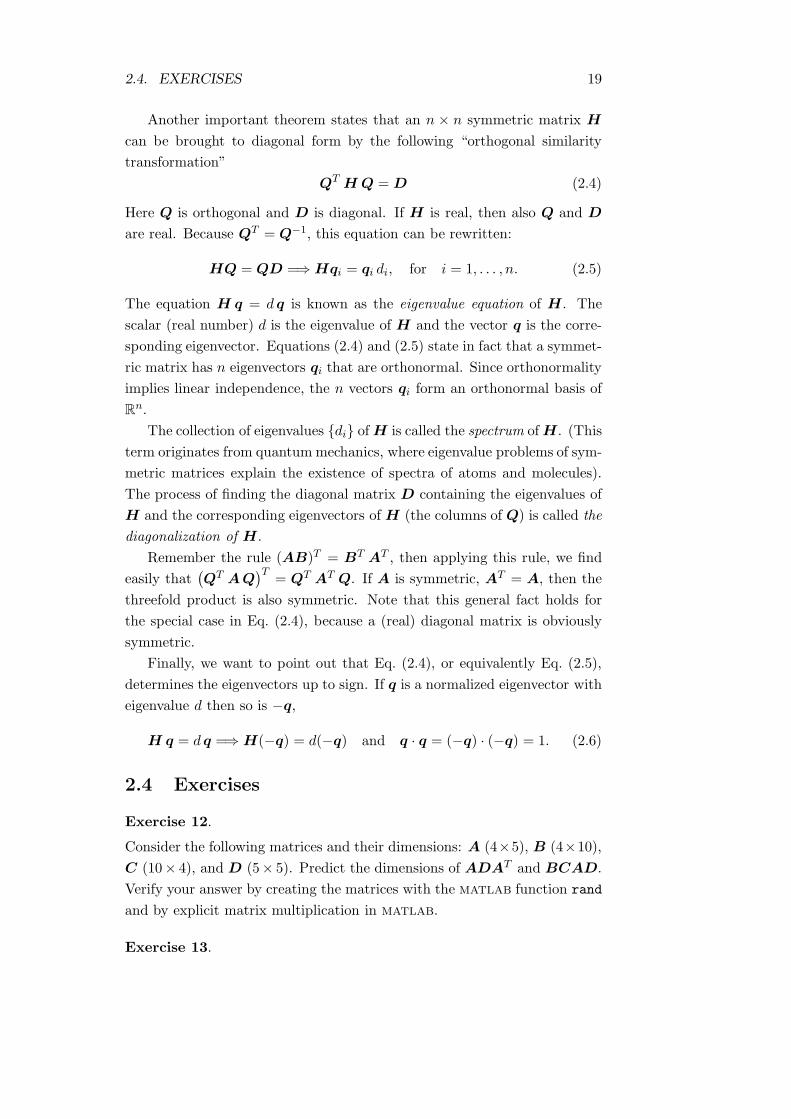
Another important theorem states that an n × n symmetric matrix H
can be brought to diagonal form by the following “orthogonal similarity
transformation”
QT HQ = D (2.4)
Here Q is orthogonal and D is diagonal. If H is real, then also Q and D
are real. Because QT = Q−1, this equation can be rewritten:
HQ = QD =⇒ Hqi = qi di, for i = 1, . . . , n. (2.5)
The equation H q = dq is known as the eigenvalue equation of H. The
scalar (real number) d is the eigenvalue of H and the vector q is the corre-
sponding eigenvector. Equations (2.4) and (2.5) state in fact that a symmet-
ric matrix has n eigenvectors qi that are orthonormal. Since orthonormality
implies linear independence, the n vectors qi form an orthonormal basis of
Rn.
The collection of eigenvalues di ofH is called the spectrum ofH. (This
term originates from quantummechanics, where eigenvalue problems of sym-
metric matrices explain the existence of spectra of atoms and molecules).
The process of finding the diagonal matrix D containing the eigenvalues of
H and the corresponding eigenvectors of H (the columns of Q) is called the
diagonalization of H.
Remember the rule (AB)T = BT AT , then applying this rule, we find
easily that(QT AQ
)T= QT AT Q. If A is symmetric, AT = A, then the
threefold product is also symmetric. Note that this general fact holds for
the special case in Eq. (2.4), because a (real) diagonal matrix is obviously
symmetric.
Finally, we want to point out that Eq. (2.4), or equivalently Eq. (2.5),
determines the eigenvectors up to sign. If q is a normalized eigenvector with
eigenvalue d then so is −q,
H q = dq =⇒ H(−q) = d(−q) and q · q = (−q) · (−q) = 1. (2.6)
2.4 Exercises
Exercise 12.
Consider the following matrices and their dimensions: A (4×5), B (4×10),
C (10× 4), and D (5× 5). Predict the dimensions of ADAT and BCAD.
Verify your answer by creating the matrices with the matlab function rand
and by explicit matrix multiplication in matlab.
Exercise 13.

20 CHAPTER 2. MATRICES
1. Enter the statements necessary to create the following matrices:
A =
1 4 62 3 51 0 4
B =
2 3 51 0 62 3 1
C =
5 1 9 04 0 6 23 1 2 4
D =
3 2 54 1 30 2 12 5 6
2. Compute the following using matlab, and write down the results. If
you receive an error message rather than a numerical result, explain
the error.
a. A+B g. C+D
b. A-2.*B h. C’+D
c. (A-2).*B i. C.*D
d. A.^2 j. A-2*eye(3)
e. sqrt(A) k. A-ones(3)
f. C’ l. A^2
Exercise 14.
Read the help of eye and ones. Create the following matrices, each with
one statement,
1 0 0 0 00 1 0 0 00 0 1 0 0
and also
1 1 11 1 11 1 11 1 11 1 1
.
Exercise 15.
The position of the center of mass of a rigid molecule consisting of n nuclei
is given by the vector
c =1
M
n∑
i=1
miri =1
M(r1 r2 · · · rn)
m1
m2...
mn
Here mi is the mass of nucleus i (mass of electrons is neglected) and ri is
the position of nucleus i, M =∑n
i=1 mi is the total nuclear mass of the
molecule.

2.4. EXERCISES 21
Consider now the isotope substituted methane CH2D2 with mC ≡ 12
u, mH ≈ 1 u, mD ≈ 2 u, where u is the unified atomic mass unit. Take a
frame (system of axes) with C in the origin and use the geometry of methane
described in exercise 6 of Sec. 1.3.
• Compute the position coordinates of the protons and the deuterons
and put these together with the position vector of carbon into a 3× 5
matrix R.
• Put the five nuclear masses into a corresponding column vector and
compute the total mass (the matlab function sum returns the sum of
the elements of a vector).
• Compute the center of mass c by matrix vector multiplication. Is the
center of mass closer to the deuterons than to the protons?
Next we translate the frame so that its origin coincides with the center of
mass. Mathematically, this is accomplished as follows
R′ ≡ R− (c c · · · c)︸ ︷︷ ︸
n times
with R ≡ (r1 r2 · · · rn)
since
R′
m1
m2...
mn
≡ (r′1 r′2 · · · r′n)
m1
m2...
mn
= R
m1
m2...
mn
− (c · · · c)
m1
m2...
mn
= Mc− c
n∑
i=1
mi = 0
or
c′ ≡ 1
M
n∑
i=1
mir′
i = 0.
• Compute the coordinates of the nuclei of CH2D2 (including the posi-
tion of carbon) with respect to the translated frame.
Hint: The translation matrix can be constructed as [c c c c c],
more elegant is by repmat(c,1,5), see help repmat.
Exercise 16.
The function reference qr(A) gives the QR decomposition of A. The function
qr(A) is an example of a matlab function that can optionally return more
than one parameter: [Q R] = qr(A) returns both the orthogonal matrix Q
and the upper triangular matrix R. Decompose A=rand(5,i) for i=1,3,5,7.
22 CHAPTER 2. MATRICES
Check in all four cases whether Q is orthogonal and inspect R to see if it is
upper triangular.
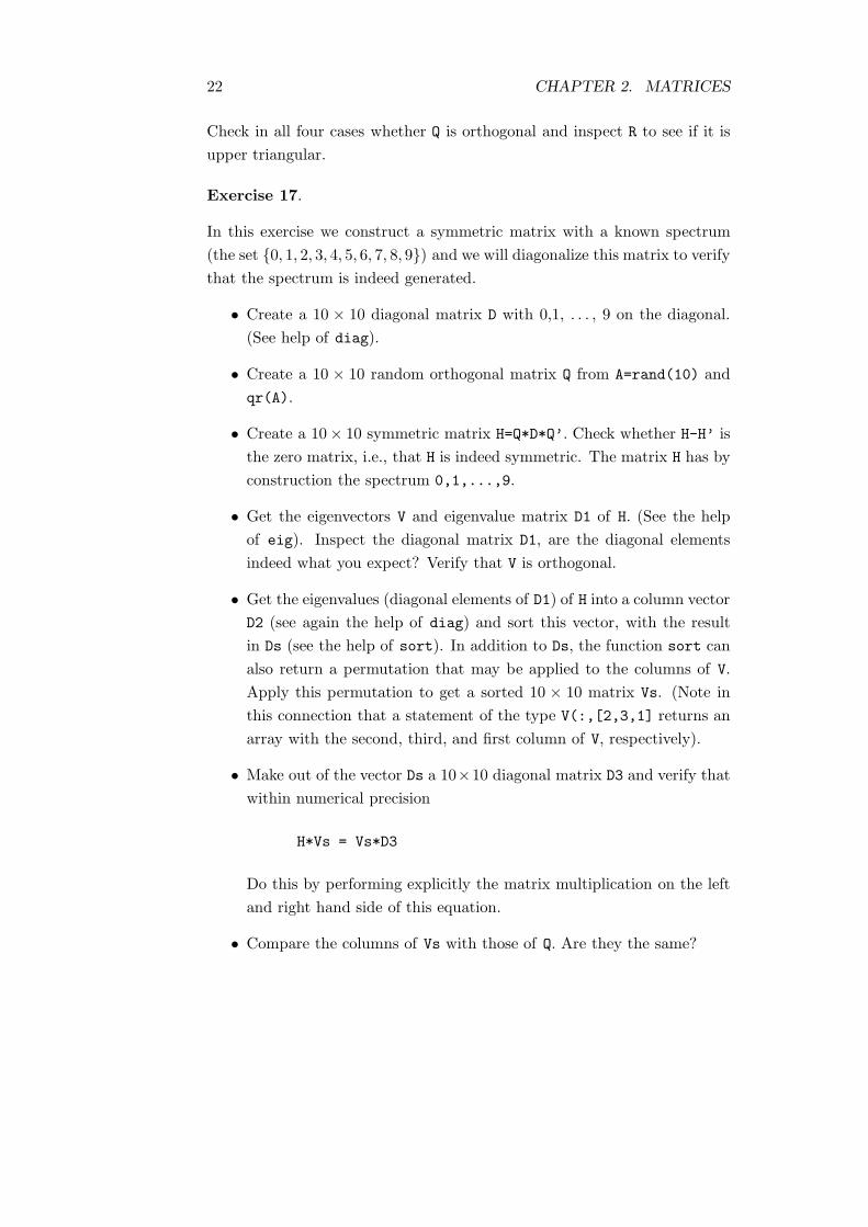
Exercise 17.
In this exercise we construct a symmetric matrix with a known spectrum
(the set 0, 1, 2, 3, 4, 5, 6, 7, 8, 9) and we will diagonalize this matrix to verify
that the spectrum is indeed generated.
• Create a 10 × 10 diagonal matrix D with 0,1, . . . , 9 on the diagonal.
(See help of diag).
• Create a 10 × 10 random orthogonal matrix Q from A=rand(10) and
qr(A).
• Create a 10× 10 symmetric matrix H=Q*D*Q’. Check whether H-H’ is
the zero matrix, i.e., that H is indeed symmetric. The matrix H has by
construction the spectrum 0,1,...,9.
• Get the eigenvectors V and eigenvalue matrix D1 of H. (See the help
of eig). Inspect the diagonal matrix D1, are the diagonal elements
indeed what you expect? Verify that V is orthogonal.
• Get the eigenvalues (diagonal elements of D1) of H into a column vector
D2 (see again the help of diag) and sort this vector, with the result
in Ds (see the help of sort). In addition to Ds, the function sort can
also return a permutation that may be applied to the columns of V.
Apply this permutation to get a sorted 10 × 10 matrix Vs. (Note in
this connection that a statement of the type V(:,[2,3,1] returns an
array with the second, third, and first column of V, respectively).
• Make out of the vector Ds a 10×10 diagonal matrix D3 and verify that
within numerical precision
H*Vs = Vs*D3
Do this by performing explicitly the matrix multiplication on the left
and right hand side of this equation.
• Compare the columns of Vs with those of Q. Are they the same?
3. Scripts and plotting
3.1 Scripts
Use of matlab editor for writing scripts.
So far we used matlab as a calculator and typed in commands on the fly
(although doubtlessly you will have discovered matlab’s history mecha-
nism). When one has to type in longer sequences of matlab commands, it
is pleasant to be able to edit and save them. Sequences of commands can
be stored in scripts. A script is a flat (ascii, plain) file containing matlab
commands that are executed one after the other. A script can be prepared
by any ascii editor, such as Microsoft’s notepad (but not by Microsoft’s
wordpad or word!). We will use the editor contained in matlab. This
editor can be started from the matlab prompt by the command edit. The
scripts must be saved under the name anyname.m, where anyname is for the
user to define.
Advice:
• Use meaningful names for your scripts, because experience shows that
you will forget very soon what a script is supposed to do.
• Save your scripts on your unix disk, this disk is backed up, whereas
your ms-windows disk is cleared after you finish working, (not at
home, of course, but in the university computer rooms).
• Mind where you are with your directories and disks. matlab shows
your current directory in the toolbar. When you are about to save a
script, the editor allows you to browse and change directories to your
unix disk before actually saving. From the matlab session you can
also browse and change directories by clicking the button to the right
of the “current directory” field.
• Let the first few lines be comments explaining the script. These com-
ments can be shown in your matlab session by help name, where
name is the name of your script.
Provided your script is in your current directory, you can execute it by simply
typing in anyname, where anyname is the meaningful name you have given
to your script. Depending on the semicolons, you will see the commands
being executed. If you have too much output on your screen you can toggle
23

24 CHAPTER 3. SCRIPTS AND PLOTTING
more on/more off. Press the “q” key to exit out of displaying the current
item.
It is important to notice that a script simply continues your matlab
session, all variables that you introduced ‘by hand’ are known to the script.
After the script has finished, all variables changed or assigned by the script
stay valid in your matlab session. Technically this is expressed by the
statement: script variables are global.
Sometimes statements in a script become unwieldily long. They can be
continued over more than one line by the use of three periods ..., as for
example
s = 1 - 1/2 + 1/3 - 1/4 + 1/5 - 1/6 + 1/7 ...
- 1/8 + 1/9 - 1/10 + 1/11 - 1/12 ...
+ 1/13 - 1/14;
Blanks around the =, +, and − signs are optional, but they improve read-
ability.
3.2 Plotting
Grids, 2D plotting.
Scripts are particularly useful for creating plots. matlab has extensive
facilities for plotting. Very often one plots a function on a discrete grid.
The matlab command for creating a grid is simple,
grid = beg:inc:end
Here beg gives the first grid value, inc the increment (default 1) and end
the end value. Example:
>> g=0:pi/10:pi
g =
Columns 1 through 5
0 0.3142 0.6283 0.9425 1.2566 1.5708
Columns 6 through 10
1.8850 2.1991 2.5133 2.8274
Column 11
3.1416
If we now want to plot the sine function on this grid we simply issue the
command plot(g, sin(g)), since the command plot(x,y) plots vector y
versus vector x. After this command a new window opens with the plot.

3.2. PLOTTING 25
Suppose we now also want to plot the cosine in the same figure. If we
would enter plot(g, cos(g)), then the previous plot would be overwritten.
We can toggle hold on/off to hold the plot. Alternatively, we can create
two plots in one statement: plot(g, sin(g), g, cos(g) ), i.e,
>> plot(x1, y1, x2, y2)
plots vector y1 versus vector x1 and y2 versus x2. Different colors and line
types can be chosen, see help plot for information on this. For example,
plot(g,cos(g), ’r:’) plots the cosine as a red dotted line. Even briefer:
plot(g’,[sin(g’) cos(g’)]) (columns of a matrix plotted against a vec-
tor).
The xlabel and ylabel functions add labels to the x and y axis of the
current figure. Their parameter is a string (is contained in quotes), thus,
e.g., ylabel(’sin(\phi)’) and xlabel(’\phi’). The title function adds
a title on top of the plot. Example:
phi=[0:pi/100:2*pi];
plot(phi*180/pi,sin(phi))
ylabel(’sin(\phi)’)
xlabel(’\phi (degrees)’)
title(’Graph of the sine function’)
For people who know the text editing system LATEX this part of matlab is
easy, since it uses quite a few of the LATEX commands. \phi is LATEX to get
the Greek letter φ. (The present lecture notes are prepared by the use of
LATEX).
In case we want to plot more than one set of y values for the same grid
of x values, matlab offers a solution. In the command plot(x,y) x is
a vector, let us say it is a column vector of length n. Then y can be an
n × k matrix (by definition consisting of k columns of length n). The plot
command gives k curves as function of the grid x.
Example:
phi=[0:pi/100:2*pi]’;
y(:,1) = cos(phi);
y(:,2) = sin(phi);
plot(phi, y)
title(’Graph of the sine and cosine functions’)
26 CHAPTER 3. SCRIPTS AND PLOTTING
3.3 Exercises
Exercise 18.
Return to exercise 4 where you were asked to find the roots (zeros) of the
polynomial
x4 − 11.0x3 + 42.35x2 − 66.550x + 35.1384.
Write a matlab script to plot this function. Define first a grid (set of
x points) with 0.6 ≤ x ≤ 4.9 and plot the function on this grid (do not
forget dots in the dot operations!). Try to find the roots of this polynomial
graphically. When you have located the roots approximately refine your
grids and try to get the roots with a two digit precision. The command
grid on is helpful, try it!
Exercise 19.
Write a matlab script that plots the functions exp(−αR) and R exp(−αR)
in one figure. Do not forget the dot (pointwise operation) at the appropriate
places! Let the first curve be solid green and the second dashdotted blue.
Assume that the grid R and the parameter α are first set by hand in the
matlab session that calls the script. Once the script is finished, experiment
with α and the grid to get a nice figure. Put to the x axis: ‘distance R (a0)’,
and use as a title ’Radial part of s and p functions’. Hint: the subscript 0
is obtained by the underscore: a_0.
Exercise 20.
Write a matlab script that plots the function
y =1
(x− 0.3)2 + 0.01+
1
(x− 0.9)2 + 0.04− 6,
which has two humps. Compute in the script first the grid 0:0.002:1 and
then the array (= vector) y and then call plot(x,y). Start the script with
the command clear all, which removes all variables from your matlab
workspace, to avoid possible side effects.
Exercise 21.
Draw a circle with radius 1 and midpoint at (0, 0).
Two possibilities (try both):
1. Make a grid for −1 ≤ x ≤ 1. Use y = ±√1− x2, compute ±y.
2. Make a grid of φ values 0 ≤ φ ≤ 2π, use x = cosφ, y = sinφ.

4. Matrices continued, flow control
4.1 Matrix sections
Sections out of matrices.
Thus far we have met twice the colon (:) operator: once to get a section
out of a matrix and once to generate a grid. In fact, these are the very same
uses of this operator. To explain this, we first observe that elements from
an array (= matrix) may be extracted by the use of an index array with
integer elements.
Example:
>> A = rand(5);
>> I = [1 3 5];
>> B = A(I,:);
>> A, B
A =
0.9501 0.7621 0.6154 0.4057 0.0579
0.2311 0.4565 0.7919 0.9355 0.3529
0.6068 0.0185 0.9218 0.9169 0.8132
0.4860 0.8214 0.7382 0.4103 0.0099
0.8913 0.4447 0.1763 0.8936 0.1389
B =
0.9501 0.7621 0.6154 0.4057 0.0579
0.6068 0.0185 0.9218 0.9169 0.8132
0.8913 0.4447 0.1763 0.8936 0.1389
Explanation:
For illustration purpose we created a 5×5 matrix A suppressing its printing.
Then we created the integer array I and used it to create an array B that
has the same columns as A but only row 1, 3, and 5 of A. Parenthetically,
note the use of the comma, we can put more than one command on a single
line: the commands must be separated by a semicolon (no printing) or a
comma (do print).
We get the very same matrix B by the command B=A(1:2:5,:), because
‘on the fly’ an array [1,3,5] is prepared and used to index A. Recall that
27
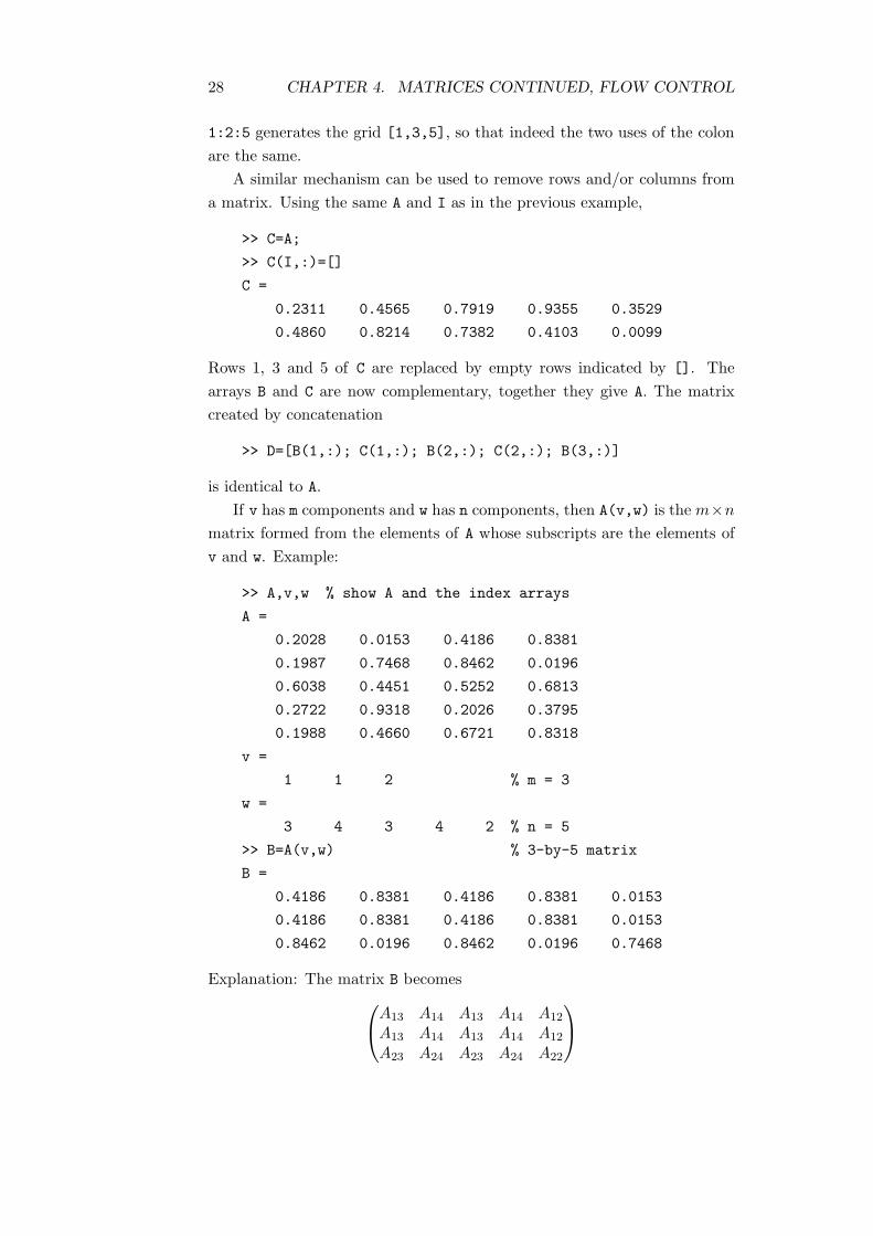
28 CHAPTER 4. MATRICES CONTINUED, FLOW CONTROL
1:2:5 generates the grid [1,3,5], so that indeed the two uses of the colon
are the same.
A similar mechanism can be used to remove rows and/or columns from
a matrix. Using the same A and I as in the previous example,
>> C=A;
>> C(I,:)=[]
C =
0.2311 0.4565 0.7919 0.9355 0.3529
0.4860 0.8214 0.7382 0.4103 0.0099
Rows 1, 3 and 5 of C are replaced by empty rows indicated by []. The
arrays B and C are now complementary, together they give A. The matrix
created by concatenation
>> D=[B(1,:); C(1,:); B(2,:); C(2,:); B(3,:)]
is identical to A.
If v has m components and w has n components, then A(v,w) is the m×n
matrix formed from the elements of A whose subscripts are the elements of
v and w. Example:
>> A,v,w % show A and the index arrays
A =
0.2028 0.0153 0.4186 0.8381
0.1987 0.7468 0.8462 0.0196
0.6038 0.4451 0.5252 0.6813
0.2722 0.9318 0.2026 0.3795
0.1988 0.4660 0.6721 0.8318
v =
1 1 2 % m = 3
w =
3 4 3 4 2 % n = 5
>> B=A(v,w) % 3-by-5 matrix
B =
0.4186 0.8381 0.4186 0.8381 0.0153
0.4186 0.8381 0.4186 0.8381 0.0153
0.8462 0.0196 0.8462 0.0196 0.7468
Explanation: The matrix B becomes
A13 A14 A13 A14 A12
A13 A14 A13 A14 A12
A23 A24 A23 A24 A22

4.2. FLOW CONTROL 29
Rows are labeled by v and columns by w. Note that elements of A can be
used more than once. This mechanism allows us, for example, to replicate
a vector:
x = % show x
1
2
3
4
5
>> X=x(:,ones(1,3)) % is the same as x([1:5],[1 1 1])
X =
1 1 1
2 2 2
3 3 3
4 4 4
5 5 5
Alternatively, we may use the matlab command repmat, which in fact uses
the same mechanism. The following command constructs the very same
matrix X: repmat(x,1,3).
4.2 Flow control
For and while loops, if then else, break.
It often happens that one wants to repeat a calculation for different values
of a parameter. To this end matlab uses the for loop. The general form of
a for statement is:
for var = expr
statement
...
statement
end
Here expr can be a rectangular array, although in practice it is usually a row
vector of the form x:y, in which case its columns are simply scalars. The
columns of expr are assigned one at a time to var and then the following
statements, up to end, are executed. For loops can be nested:
A=zeros(10,5);
for i = 1:10
for j = 1:5

30 CHAPTER 4. MATRICES CONTINUED, FLOW CONTROL
A(i,j) = 1/(i+j-1);
end
end
In a situation as in this example it helps matlab a lot if it knows in advance
how large a matrix is going to be. It saves much computer time if the loops
in the previous example are preceded by the command which initializes A to
a 10 × 5 matrix, (which are here taken to be zeros, but ones(10,5) would
have done as well).
As an example where columns are used as loop variables we flip the
columns of A
A=rand(5,3);
B=zeros(5,3);
i=4;
for a=A % a runs from column 1 upwards to column 3
i=i-1; % i counts down
B(:,i) = a;
end
(This loop is achieved in one statement by the matlab function fliplr
which issues a statement similar to B=A(:,3:-1:1)).
The break statement can be used to terminate the loop prematurely. To
explain this we first need to discuss the if expression.
Leaving aside some sophisticated array indexing situations, matlab be-
haves most of the time as if it does not know logical (boolean) variables.
matlab uses non-zero for true and zero for false. The comparison operator
is ==, i.e., a==b yields non-zero (1) if a and b are equal and 0 otherwise:
>> 1==2
ans =
0
>> 1==1
ans =
1
The function disp can be used to display strings and the following state-
ments illustrate the use of if
>> if pi disp(’yes’), end % pi=3.14.. is non-zero
yes % output of disp
>> if 0 disp(’yes’), end % no output

4.2. FLOW CONTROL 31
The keyword if needs a corresponding end.
The general syntax of the if statement is
if expression
statements
elseif expression
statements
else
statements
end
The statements are executed if the expression has all non-zero elements.
The else and elseif parts are optional. Zero or more elseif parts can be
used as well as nested ifs. The expression is usually of the form
expr rop expr
where the relational operator rop is:
== equal< less than> greater than<= less or equal>= greater or equal~= not equal
We return now to the break command which terminates execution of a
for (and while) loop. In nested loops, break exits from the innermost loop
only. As an example we suppose that we have an array with a number of
positive elements followed by negative elements. We want to take square
roots of the positive elements only.
V=[rand(5,1); -rand(4,1)]; % a column
i = 0;
for v=V’ % here we want a row
if v >= 0, i = i+1; w(i)=sqrt(v);
else break
end % end of if
end % end of for loop
i % break jumps to here
An alternative solution of the same problem is with the while loop:

32 CHAPTER 4. MATRICES CONTINUED, FLOW CONTROL
V=[rand(5,1); -rand(4,1)];
i = 1;
v = V(1);
while v >=0 % returns zero(false) or non-zero(true)
w(i)=sqrt(v);
i = i+1;
v = V(i);
end
v % v is negative here!
Explanation:
The command while repeats statements up to end an indefinite number of
times. The general form of a while statement is:
while expr
statements
....
statements
end
The statements in the body of the while loop are executed as long as the
expr has only non-zero elements. Usually expr is a logical expression that
results in 0 or 1. As soon as expr becomes 0 the loop is quitted.
4.3 Exercises
Exercise 22.
What is the value of i printed as last statement of the following script?
V=[rand(2,1); -rand(2,1); rand(2,1); -rand(2,1)]
i = 1;
v = V(i);
while v >= 0
i = i+1;
v = V(i);
end
i
Exercise 23.
4.3. EXERCISES 33
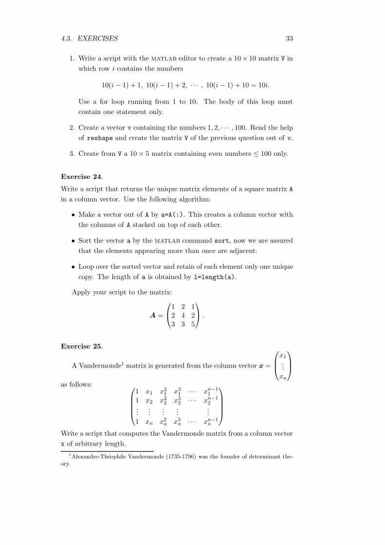
1. Write a script with the matlab editor to create a 10× 10 matrix V in
which row i contains the numbers
10(i − 1) + 1, 10(i− 1) + 2, · · · , 10(i − 1) + 10 = 10i.
Use a for loop running from 1 to 10. The body of this loop must
contain one statement only.
2. Create a vector v containing the numbers 1, 2, · · · , 100. Read the help
of reshape and create the matrix V of the previous question out of v.
3. Create from V a 10× 5 matrix containing even numbers ≤ 100 only.
Exercise 24.
Write a script that returns the unique matrix elements of a square matrix A
in a column vector. Use the following algorithm:
• Make a vector out of A by a=A(:). This creates a column vector with
the columns of A stacked on top of each other.
• Sort the vector a by the matlab command sort, now we are assured
that the elements appearing more than once are adjacent.
• Loop over the sorted vector and retain of each element only one unique
copy. The length of a is obtained by l=length(a).
Apply your script to the matrix:
A =
1 2 12 4 23 3 5
.
Exercise 25.
A Vandermonde1 matrix is generated from the column vector x =
x1...xn
as follows:
1 x1 x21 x31 · · · xn−11
1 x2 x22 x32 · · · xn−12
......
......
...1 xn x2n x3n · · · xn−1
n
Write a script that computes the Vandermonde matrix from a column vector
x of arbitrary length.
1Alexandre-Theophile Vandermonde (1735-1796) was the founder of determinant the-ory.

34 CHAPTER 4. MATRICES CONTINUED, FLOW CONTROL
Hint:
This script does not need more than three statements if we use cumprod;
see its help.
Exercise 26.
You may have noticed that the description above of the if elseif else
end construction was very brief. In particular it was not explained what
happens if conditions in different elseifs are simultaneously true. Look at
the following three programs and predict what they put on the screen.
a=-3; | a=-3; | a=-3;
if a < -5 | if a < -5 | if a < -3
disp(’ < -5 ’) | disp(’ < -5 ’) | disp(’ < -3 ’)
elseif a < -2 | elseif a < -1 | elseif a < -4
disp(’ < -2 ’) | disp(’ < -1 ’) | disp(’ < -4 ’)
elseif a < -1 | elseif a < -2 | elseif a < -5
disp(’ < -1 ’) | disp(’ < -2 ’) | disp(’ < -5 ’)
else | else | else
disp(’rest’) | disp(’rest’) | disp(’rest’)
end | end | end
Make a script out of the first program and verify your prediction. Then edit
this script to get the second program and verify again, and do this also for
the third program.
Exercise 27.
In quantum mechanics the angular momentum operators lx, ly, lz play an
important role. Also l+ ≡ lx+ily and l− ≡ lx−ily are often considered. The
latter operators are represented by (2l + 1)× (2l + 1) matrices with indices
m = −l, . . . , l and m′ = −l, . . . , l. They are defined by
(L±)mm′ = δm,m′±1
√
l(l + 1)−m′(m′ ± 1)
That is, L+ is almost completely zero with only non-zero elements on the
diagonal above the main diagonal. Likewise, L− has only elements on the
diagonal below the main diagonal.
1. Compute the two vectors s± =√
l(l + 1)−m(m± 1) for l = 5 and
m = −5, . . . 5. Both vectors are of length 2l + 1.
2. Read the help of diag and construct from the two vectors s± the
matrices L+ and L− by means of diag.
4.3. EXERCISES 35
Hint: The lower diagonal matrix L− starts at (m,m′) = (−l+ 1,−l)
and ends at (m,m′) = (l, l − 1), whereas the upper diagonal matrix
L+ starts at (m,m′) = (−l,−l + 1) and ends at (m,m′) = (l − 1, l).
This means that the first and last element, respectively, of the vectors
s− and s+ must not be used in the command diag.
3. Compute Lx = (L+ +L−)/2 and Ly = (L+ −L−)/(2i).
Hint: Compute the imaginary number i by√−1.
4. Compute i(LxLy −LyLx
). Do you recognize the result?

36 CHAPTER 4. MATRICES CONTINUED, FLOW CONTROL

5. Least squares fitting
5.1 Linear equations
Linear equations, backslash operator.
Consider the square system of n linear equations with n unknowns x1, · · · , xn,
A11x1 +A12x2 + · · ·A1nxn = y1
A21x1 +A22x2 + · · ·A2nxn = y2
· · · · · · · · ·An1x1 +An2x2 + · · ·Annxn = yn
or more compactly
Ax = y where A is n× n, x and y are n× 1. (5.1)
Here A and y are known and x must be solved. We already met the matrix
function inv. This function computes the inverse of a non-singular matrix.
One solution would be therefore to write simply x = inv(A)*y. Since in-
verting a matrix is in fact equivalent to solving n times a system of n linear
equations with the n columns of the identity matrix playing the role of the
right hand sides y, it is clear that inversion of A is usually too expensive
in terms of computer time. matlab can solve the system in one statement:
x=A\y. Here we meet for the first time the backslash operator (\). This
operator has much similarity with the slash operator (/). A quantity hiding
under the slash is inverted, thus 1/5=0.200 and
(1 1
)/
(5 00 2
)
≡(1 1
)(5 00 2
)−1
=(1/5 1/2
).
This reads in matlab
>> [1 1]/[5 0; 0 2]
ans =
0.2000 0.5000
(Remember that the inverse of a diagonal matrix is again a diagonal matrix
with the inverses of the diagonal elements on the diagonal). In the very same
37

38 CHAPTER 5. LEAST SQUARES FITTING
way a quantity hiding under the backslash is inverted, thus 5\1=0.200. The
equation(5 00 2
)−1 (11
)
=
(1/51/2
)
reads in matlab
>> [5 0; 0 2]\ [1; 1]
ans =
0.2000
0.5000
So, as long as the matrix A in Eq. (5.1) is non-singular, the solution of linear
equations is straightforward: if a column vector x must be solved we use the
backslash and if a row vector x must be solved we use the ordinary slash,
Ax = y =⇒ x = A\y (multiplication with A−1 on the left)
xTA = yT =⇒ xT = yT /A (multiplication with A−1 on the right)
5.2 Least squares
Linear least squares, pseudo inverse.
A system of linear equations cannot be solved so straightforwardly when
its coefficient matrix is non-square. Most often one meets m× n coefficient
matrices with m > n in linear fits. To explain this we first discuss curve
fitting (also known as regression).
Suppose we have a measurable quantity y which is a function of x. (For
instance, y can be the pressure of a gas and x its temperature. Or y can
be the torsion energy associated with rotation of a methyl group around a
bond in a molecule; then x is the torsion angle.)
Assume that we have measuredm values y1, y2, . . . , ym for x1, x2, . . . , xm,
respectively. Very often one wants to find a curve f(x) that passes as well
as possible through the points, i.e, f(xi) must be as close as possible to yi,
for all i = 1, . . . ,m. One then guesses a family of functions fα1,α2,...,αn(x),
of which the family members only differ in the fit parameters α1, α2, . . . , αn.
A simple example of a four parameter family of fit functions is
fα1,α2,α3,α4(x) = α1 exp(−α2x
2) + α3 exp(−α4x2).
This function depends linearly on α1 and α3, these are the linear fit param-
eters, and exponentially on α2 and α4 (non-linear fit parameters). The least

5.2. LEAST SQUARES 39
squares fitting problem is the determination of the parameters of a chosen
fit function f such that the sum of squares is least, i.e.,
[m∑
i=1
(f(xi)− yi
)2
]1/2
is a minimum. (5.2)
This condition becomes clearer if we introduce the vector
f ≡(f(x1), f(x2), . . . , f(xm)
)
and a vector containing the experimental results
y ≡(y1, y2, . . . , ym
).
Now condition (5.2) reads that the norm of the difference vector f −y must
be as small as possible, or in other words, the vector f must be as close as
possible to the vector y. Both vectors are in Rm.
The problem of determining non-linear fit parameters is difficult, often
one meets different local minima in |f − y| as function of these parameters
and the global minimum is not always physically meaningful.
The determination of linear parameters on the other hand is easy and
can be performed by one matlab statement. So we will concentrate on
linear fitting. First one chooses a linear expansion basis χ1(x), . . . , χn(x).
The choice of this basis depends on the problem at hand. For instance in the
case of torsion energy, which is periodic with period 2π, one would choose
cos kφ and sin k′φ as the expansion basis with k, k′ = 0, 1, 2, . . .. Gaussian
functions are often used χi(x) = exp(−αix2), provided the exponents αi are
known, otherwise we have a non-linear fitting problem. Most often one uses
powers of x, χi(x) = xi, so that the expansion becomes a polynomial [first
terms of the Taylor series of y(x)]. In any case we write
f(x) = c1χ1(x) + c2χ2(x) + · · ·+ cnχn(x) =
n∑
j=1
cjχj(x),
where the cj are the linear fit parameters to be determined by minimizing
|f − y|. Consider f in the point xi,
f(xi) =
n∑
j=1
χj(xi)cj , i = 1, . . . ,m.
Introducing the matrix element Aij ≡ χj(xi) and fi ≡ f(xi) we have
fi =n∑
j=1
Aijcj =⇒ f = Ac.

40 CHAPTER 5. LEAST SQUARES FITTING
The functions χi(x) are known, we assume that we know the points xi at
which the measurements are performed and hence we can compute them×n
matrix A. Usually we have many more measurements than fit parameters:
m ≫ n. We do not know f , but we want it to be as close as possible to the
known (measured) vector y.
Minimization of |f − y| leads to the n equations
AT Ac = ATy. (5.3)
These are known as the normal equations of the linear least square problem.
Before proceeding we prove Eqs. (5.3). We minimize S ≡ |f − y|2 (which
obviously has the same minimum as |f −y|) with respect to ci, i = 1, . . . , n,
i.e., we put the first derivatives equal to zero. By invoking the chain rule we
get:
∂S
∂ci=
∂
∂ci
m∑
j=1
(fj − yj)2 = 2
m∑
j=1
∂fj∂ci
(fj − yj). (5.4)
Now,
∂fj∂ci
=∂
∂ci
n∑
k=1
Ajkck =
n∑
k=1
Ajkδki = Aji ≡ ATij, (5.5)
where we used ∂ck/∂ci = δki. Note that δki, with k running and i fixed, gives
zero always, except for k = i, in that case we get Aji × 1. The Kronecker
delta ‘filters’ from the sum over k only the k = i term. Substitute Eq. (5.5)
into Eq. (5.4) and put the derivatives equal to zero
0 =∂S
∂ci= 2
m∑
j=1
ATij(fj − yj),
or, using f = Ac,
AT f = AT y =⇒ AT Ac = ATy.
Strictly speaking, we must consider next the second derivatives to check
whether we have a minimum, saddle point or maximum, but we skip this
part of the proof1.
The matrix AT is n × m and A is m × n, so their product is square:
n× n. The vector ATy is of dimension n. If the expansion functions χi(x)
are linearly independent and the points xi are well chosen (not too close to
each other), then the matrix A is of rank n, i.e., its n columns are linearly
independent. The n × n matrix ATA is non-singular if and only if A is of
1The second derivatives lead to consideration of ATA. This matrix is positive definite
(has only positive eigenvalues) and therefore we have a minimum.

5.2. LEAST SQUARES 41
rank n. If A is of rank n then c = (ATA)−1AT y is a unique solution. We
conclude that the normal equations have a unique solution, irrespective of
the fact whether y depends linearly on the columns of A, as long as the
columns of A are linearly independent.
The n×m matrix B ≡ (ATA)−1AT is the pseudo inverse of A, because,
obviously BA = In×n. Note that AB 6= Im×m. The matrix B is also
known as the Moore-Penrose inverse of A. For the special case that A is
non-singular (and hence square), it is easily seen that B = A−1.
Returning to matlab we first note that the command pinv(A) returns
the pseudo inverse of A. So, the equation Ac = y can be solved in the least
squares sense by c = pinv(A)* y. However, it can be shorter, because the
backslash operator performs in fact pseudo inversion, c = A\y gives the
same result.
Example:
We first generate an arbitrary 3× 2 matrix A consisting of integers between
0 and 10:
>> A = fix(10*rand(3,2))
A =
9 4
2 8
6 7
The function fix rounds a floating point number down to the nearest integer,
e.g., fix(9.9) = 9. Recall that rand returns random numbers between 0
and 1. Next we compute the pseudo inverse:
>> B=pinv(A)
B =
0.0401 -0.1492 0.1050
0.0110 0.1657 -0.0055
>> B*A % To check for the identity matrix
ans =
1.0000 0
0.0000 1.0000
>> A*B % No identity?
ans =
0.2044 0.0663 0.3978
0.0663 0.9945 -0.0331
0.3978 -0.0331 0.8011

42 CHAPTER 5. LEAST SQUARES FITTING
>> y = rand(3,1) % Make a right hand side
y =
0.4057
0.9355
0.9169
>> B*y
ans =
-0.0270
0.1545
>> A\y
ans =
-0.0270
0.1545
An example of fitting a straight line through data that are made some-
what noisy:
% Synthesize data:
% Straight line, slope 3/2, 10% noise.
>> x=[1:25]’; % simple x values
>> r=rand(25,1)-0.5; % -0.5 < random < 0.5
>> y=1+3/2*(x+r.*x/10);
% The actual fit:
>> A=[x.^0 x.^1]; % f(x) = c(1) + c(2)*x
>> c=A\y % c(1) is intercept, c(2) is slope
% Plot fit and original:
>> plot(x,y, x, A*c); % (x,y) original, (x, A*c) fitted
5.3 Necessity of least squares
Linear least square equations are overdetermined.
One could be tempted to make the approximation f ≈ y in the linear model
f = Ac. This leads to a set of linear equations
y = Ac, (5.6)
where the m × n matrix A is rectangular, m > n. When we write the
columns of A as a1, . . . ,an, this set of equations is equivalent to
y = c1a1 + c2a2 + · · ·+ cnan (columns of length m).

5.3. NECESSITY OF LEAST SQUARES 43
From this we see clearly that the column vector y must depend linearly
on the columns of A in order that the approximation f ≈ y makes sense.
Usually this is not the case, of course, and then these equations do not have a
solution; simplification of the equations by elementary row transformations
will lead to contradictory equations.
In order to show this, we try to solve the equations (5.6) by the usual
techniques for solving linear equations. That is, we consider the augmented
matrix [A, y] and by elementary row transformations we “sweep” this ma-
trix to its simplest form. matlab has the command rref to do this. Using
A and y of the previous example, we get
>> rref([A, y]) % A and y as in the previous example
ans =
1 0 0
0 1 0
0 0 1
0 0 0
...
0 0 0
(the last 22 rows contain only zeros). Hence the first two equations of
Ac = y are equivalent to
(1 00 1
)(c1c2
)
=
(00
)
which have the solution c1 = c2 = 0. The third equation is equivalent to
0 = 1. From this contradiction we conclude that, although the linear least
square solution c is uniquely determined, the equations Ac = y have no
solution in the ordinary sense. Or in other words, the three vectors a1, a2
and y are linearly independent. (This is due to the addition of noise, if we
had simply put y = 1 + 3x/2, y would have been the first column plus a
multiple of the second column of A, and the three vectors would have been
linearly dependent).
Suppose now that y depends linearly on the columns of A. This means
that there is a vector d = (d1, d2, . . . , dn) of length n such that
y = d1a1 + d2a2 + · · ·+ dnan = Ad,
where ai is the ith column of A. These columns are of length m. It is
immediately obvious that the least square solution c gives the correct answer,
for
c = (ATA)−1AT y = (ATA)−1AT Ad = d.
44 CHAPTER 5. LEAST SQUARES FITTING
If we had written y = 1+3x/2 in the example above, without adding noise,
we would have found c(1) = 1 and c(2) = 3/2. The corresponding least
squares solution y = 1 + 3x/2 gives back exactly what we put in. In that
sense the method of least squares is stable.
5.4 Exercises
Exercise 28.
Visit for this exercise
http:/www.theochem.kun.nl/~pwormer,
where you find a link to course material. Follow this link and click the
link heatH2O.txt and an ascii file containing comments and two columns
is opened. The columns are temperatures (C) and heat capacities Cp of
steam at 1 atm [units: Cal/(C g)]. Save this file in your current directory
(most browsers have this option under their File button).
matlab can read ascii files that contain columns and skips comments
while reading. Issue the command load heatH2O.txt in your matlab ses-
sion. You now have an array heatH2O containing the two columns. (The
command: load arr.any creates an array with the name of the string be-
fore the dot—in this case arr—and discards the arbitrary string after the
dot). Create a column vector T containing the temperatures and the column
vector Cp containing the heat capacities.
• Perform a quadratic fit Cp ≈ c1 + c2T + c3T2 and compute the error
(norm of the vector containing the differences between the original and
the fitted points). Plot the fitted and the original values as a function
of temperature.
• Perform a cubic fit Cp ≈ d1 + d2T + d3T2 + d4T
3 and compute the
error (norm of the difference vector). Which of the two fits has the
smaller error? Plot also this fit.
• Use both fits to extrapolate the heat capacity to 750 and 1000 C. Plot
the fits in one figure including the extrapolated points. Which of the
two fits give extrapolated values closest to the real value, you think?
Exercise 29.
The linear parameters obtained in a least squares fit can be given statistical
significance. Write ν ≡ m−n for the number of degrees of freedom (number
5.4. EXERCISES 45
of measurements m minus number of fit parameters n). The measure for
the fit error: s2e ≡ 1ν |f − y|2 appears in the variance-covariance matrix
V = s2e(ATA)−1 ,
where Aij = xji , i = 1, . . . ,m, j = 0, . . . , n−1, (xji is xi to the power j). The
vector y contains the measured values and f the fitted ones. The estimated
standard deviation si of the fit coefficient ci is given by√Vii. The 95%
confidence interval for fit parameters c = (c1, . . . , cn) can now be obtained
from
ci ± t0.05,νsi,
where t0.05,ν is an entry in Student’s t-table2. Recall that the rows and
columns of a t-table are given by confidence levels (here 0.05) and number
of degrees of freedom (ν). If ci−t0.05,νsi ≤ 0 ≤ ci+t0.05,νsi, then the variable
ci is not significantly different from zero.
Confidence intervals for interpolating predictions can be calculated as
well. Consider x0 = (x10, x20, . . . , xm0)T , a column vector consisting of m
points spanning the same range as the x-values of the measurements. These
points interpolate the x-values of the measurements. Consider the m × n
matrix
X0 =
1 x10 x210 · · · xn−110
......
...
1 xm0 x2m0 · · · xn−1m0
.
Then the 95% confidence interval at point xi0 is
fi0 ± t0.05,ν
√(X0 V XT
0
)
ii, i = 1, . . . ,m,
where f0 ≡ X0c, (a column vector of length m), interpolates the measured
values.
Take care not to confuse this interval with a prediction interval for a
single measurement, which is given by
fi0 ± t0.05,ν
√
s2e +(X0 V XT
0
)
ii.
Note that prediction intervals are wider than confidence intervals.
After this preamble consider again the data from the previous Exercise
(file heatH2O.txt).
2Discovered by William Sealy Gosset (1876–1937), who was employed by Guinnessbreweries in Dublin. Guinness encouraged their employees to publish under pseudonyms;Gosset chose ‘Student’.

46 CHAPTER 5. LEAST SQUARES FITTING
• Perform again the quadratic fit Cp ≈ c1 + c2T + c3T2. Calculate the
standard deviations si of the coefficients. Are all coefficients signifi-
cantly different from zero? Form an equidistant grid of 100 tempera-
ture points (see help linspace) spanning the same range as the input
points. Compute the 95% confidence intervals where you can take
t0.05,ν = 2. Plot the fitted values, confidence intervals and original
values (dashed) in one figure.
• For the same 100 points, calculate the prediction intervals for a single
measurement (i.e., within what values would you expect one single
measurement to be the outcome for 95% of the time)? Plot these in
the same figure as dotted lines.
Exercise 30.
Visit for this exercise
http:/www.theochem.kun.nl/~pwormer.
Follow the link to the course material. When you click O2.txt an ascii
file containing comments and two columns is opened. The columns are
interatomic distances (bohr) and energies (hartree) for the oxygen molecule
O2. Save this file in your current directory. See previous exercise for more
details on how to do this.
• Write a script that loads the oxygen file into your matlab session
and fits the energies as function of the distance r with the following
function: V ≈ D0 + D1 exp(−βr) + D2 exp(−2βr). The linear fit
parameters D0, D1 and D2 can be obtained by the backslash operator.
Use β = 1. Plot the fit and the original data.
• To determine the nonlinear fit parameter β modify the script. Put
a loop with 0.8 ≤ β ≤ 1.8 with steps of 0.1 around the linear fit.
Compute in the body of the loop the norm of the difference vector
V − Vfit (original and fitted values) and determine the value of β
which has the smallest norm. Plot for this β again the original and
fitted values.
6. Functions and function
functions
6.1 Functions
Difference between scripts and functions, subfunctions.
Functions resemble scripts: both reside in an ascii file with extension .m.
As a matter of fact, many of the matlab functions that we used so far are
simply .m files. One can inspect them by the command type, e.g., type
fliplr will type the content of fliplr.m. The difference between scripts
and functions is that all variables in scripts are global, whereas all variables
in functions are local. This means that variables inside functions lead their
own life. Say, we have assigned the value −1.5 to the variable D in our
matlab session and we call a function that also assigns a value to a variable
called D. Upon return from the function the variable D still has the value
−1.5. Conversely, D must be assigned a value inside the function before it
can be used. The function does not know that D already has a value in our
matlab session.
If both are stored in an .m file, how does matlab tell the difference
between a script and a function? This is a good question with a simple
answer: the very first word of a function is function. So, when matlab
reads an .m file from disk, it looks at the first string and decides from this
whether it is a function or a script.
If all variables in a function are local, what is the use of a function? One
would like to get something useful out of a function, as for instance an array
with its columns flipped. In other words, how does a function communicate
with its environment? To explain this we give the syntax of the first line of
a function:
function [out1, out2, ...] = name(in1, in2, ...)
The first observation is that a function accepts input arguments between
round brackets. Any number (including zero) of variables can be written
here. These variables can be of any type: scalars, matrices (and matlab
objects that we have not yet met). The second observation is that a function
returns a number of output parameters in square brackets. The values of
out1, out2, etc. must be assigned within the function. These variables can
also be of any type. The square brackets here have nothing to do with the
47
48 CHAPTER 6. FUNCTIONS AND FUNCTION FUNCTIONS
concatenation operators that made larger matrices from smaller ones. The
third observation is that the function has a name. It is common to use here
the same name as of the .m file, but this is not compulsory. The name of an
.m file begins with an alphabetic character, and has a filename extension of
.m. The .m filename, less its extension, is what matlab searches for when
you try to use the script or function.
For example, assume the existence of a file on disk called stat.m and
containing:
function [mean,stdev] = stat(x)
n = length(x);
mean = sum(x)/n;
stdev = sqrt(sum((x-mean).^2)/n);
This defines a function called stat that calculates the mean and standard
deviation of the components of a vector. We emphasize again that the
variables within the body of the function are all local variables. We can call
this function in our matlab session in three different ways:
>> stat(x) % no explicit assignment
ans = % default assignment to ans
0.0159
>> m = stat(x) % assignment of first output parameter
m =
0.0159
>> [m, s] = stat(x) % assignment of both output parameters
m =
0.0159
s =
1.0023
Note that m and s are not concatenated to a 1 × 2 matrix; the square
brackets do not act as concatenation operators in this context, i.e., to the
left of the assignment sign. Notice that the concatenation operators[ and ]
only appear on the right hand sides of assignments.
A subfunction, visible only to the other functions in the same file, is
created by defining a new function with the function keyword after the body
of the preceding function or subfunction. For example, avg is a subfunction
within the file stat.m:

6.2. FUNCTION FUNCTIONS 49
function [mean,stdev] = stat(x)
n = length(x);
mean = avg(x,n);
stdev = sqrt(sum((x-avg(x,n)).^2)/n);
function [mean] = avg(x,n)
mean = sum(x)/n;
Subfunctions are not visible outside the file where they are defined. Also,
subfunctions are not allowed in scripts, only inside other functions. Func-
tions normally return when the end of the function is reached. We may
use a return statement to force an early return from the function. When
matlab does not recognize a function by name, it searches for a .m file of
the same name on disk. If the function is found, matlab stores it in parsed
form into memory for subsequent use. In general, if you input the name of
something to matlab, the matlab interpreter does the following: It checks
to see if the name is a variable. It checks to see if the name is a built-in
function (as, for instance, sqrt or sin). It checks to see if the name is a
local subfunction. When you call an .m file function from the command line
or from within another .m file, matlab parses the function and stores it
in memory. The parsed function remains in memory until cleared with the
clear command or you quit matlab.
6.2 Function functions
Function functions, function handles.
matlab has a number of functions that work through functions. This
sounds cryptic, so let us give an example immediately. The built-in function
fminsearch performs minimization. It finds minima of non-linear functions
of one or more variables. It does not apply constraints. That is, the search
for minima is on the whole real axis (or complex plane as the case maybe).
We invoke this function by
X = fminsearch(@fun,X0)
The search starts at X0 and finds a local minimum of fun at the point X. It
is our duty to supply the function fun. The function must accept the input
X, and must return the scalar function value fun evaluated at X. The input
variable X can be a scalar, vector or matrix.
Suppose we want to find the local minima of the following function:
function [y] = hump(x)
% We use dot operations so that hump may be called
% with a vector, e.g., for plotting.
y = 1 ./ ((x-0.3).^2 + 0.01) + 1 ./ ((x-0.9).^2 + 0.04) - 6;
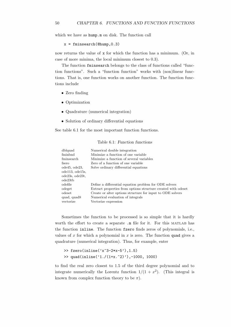
50 CHAPTER 6. FUNCTIONS AND FUNCTION FUNCTIONS
which we have as hump.m on disk. The function call
x = fminsearch(@hump,0.3)
now returns the value of x for which the function has a minimum. (Or, in
case of more minima, the local minimum closest to 0.3).
The function fminsearch belongs to the class of functions called “func-
tion functions”. Such a “function function” works with (non)linear func-
tions. That is, one function works on another function. The function func-
tions include
• Zero finding
• Optimization
• Quadrature (numerical integration)
• Solution of ordinary differential equations
See table 6.1 for the most important function functions.
Table 6.1: Function functions
dblquad Numerical double integrationfminbnd Minimize a function of one variablefminsearch Minimize a function of several variablesfzero Zero of a function of one variableode45, ode23, Solve ordinary differential equationsode113, ode15s,ode23s, ode23t,ode23tbodefile Define a differential equation problem for ODE solversodeget Extract properties from options structure created with odesetodeset Create or alter options structure for input to ODE solversquad, quad8 Numerical evaluation of integralsvectorize Vectorize expression
Sometimes the function to be processed is so simple that it is hardly
worth the effort to create a separate .m file for it. For this matlab has
the function inline. The function fzero finds zeros of polynomials, i.e.,
values of x for which a polynomial in x is zero. The function quad gives a
quadrature (numerical integration). Thus, for example, enter
>> fzero(inline(’x^3-2*x-5’),1.5)
>> quad(inline(’1./(1+x.^2)’),-1000, 1000)
to find the real zero closest to 1.5 of the third degree polynomial and to
integrate numerically the Lorentz function 1/(1 + x2). (This integral is
known from complex function theory to be π).

6.3. COUPLED FIRST ORDER DIFFERENTIAL EQUATIONS 51
The symbol @fun returns a function handle on fun. A function handle
contains all the information about a function that matlab needs to execute
that function. As we saw above, a function handle is passed in an argument
list to other functions. The receiving functions can then execute the function
through the handle that was passed in. You can, for example, execute a
subfunction using a function handle, as long as the handle was created within
the subfunction’s .m file. That is, the following construction is allowed,
where model is a subfunction of fit
function fit
...
fminsearch@model,x % create function handle
...
function model(x) % subfunction in same m file
...
The subfunction model is visible to fminsearch.
The function handle is the first matlab data type that we meet which
is not a matrix. You can manipulate and operate on function handles in the
same manner as on other data types. Function handles enable you to do the
following: (i) Pass function access information to other functions. (ii) Allow
wider access to subfunctions. (iii) Reduce the number of files that define
your functions.
6.3 Coupled first order ordinary differential equa-
tions
Coupled differential equations, chemical kinetics
matlab has several ordinary differential equation solvers (ODE solvers, see
help ode45). An ordinary differential equation has only one parameter,
which often is the time t. We will restrict ourselves in this section to first
order equations, i.e., equations containing only first derivatives with respect
to t. Usually differential equations are coupled and have the following gen-
eral form,
dy1/dt
dy2/dt
. . .
dyn/dt
=
f1(t,y(t)
)
f2(t,y(t)
)
. . .
fn(t,y(t)
)
, (6.1)
here y(t) =(y1(t), y2(t), . . . , yn(t)
)is to be computed by matlab from a
given initial vector y(t0). The functions f1, f2, . . . , fn are known and must
be supplied by the user. The ODE solver most often used is ode45. It is
called as
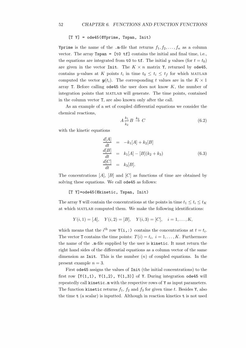
52 CHAPTER 6. FUNCTIONS AND FUNCTION FUNCTIONS
[T Y] = ode45(@Yprime, Tspan, Init)
Yprime is the name of the .m-file that returns f1, f2, . . . , fn as a column
vector. The array Tspan = [t0 tf] contains the initial and final time, i.e.,
the equations are integrated from t0 to tf. The initial y values (for t = t0)
are given in the vector Init. The K × n matrix Y, returned by ode45,
contains y-values at K points ti in time t0 ≤ ti ≤ tf for which matlab
computed the vector y(ti). The corresponding t values are in the K × 1
array T. Before calling ode45 the user does not know K, the number of
integration points that matlab will generate. The time points, contained
in the column vector T, are also known only after the call.
As an example of a set of coupled differential equations we consider the
chemical reactions,
Ak1
k2B
k3→ C (6.2)
with the kinetic equations
d[A]
dt= −k1[A] + k2[B]
d[B]
dt= k1[A]− [B](k2 + k3) (6.3)
d[C]
dt= k3[B].
The concentrations [A], [B] and [C] as functions of time are obtained by
solving these equations. We call ode45 as follows:
[T Y]=ode45(@kinetic, Tspan, Init)
The array Y will contain the concentrations at the points in time t1 ≤ ti ≤ tK
at which matlab computed them. We make the following identifications:
Y (i, 1) = [A], Y (i, 2) = [B], Y (i, 3) = [C], i = 1, . . . ,K,
which means that the ith row Y(i,:) contains the concentrations at t = ti.
The vector T contains the time points: T (i) = ti, i = 1, . . . ,K. Furthermore
the name of the .m-file supplied by the user is kinetic. It must return the
right hand sides of the differential equations as a column vector of the same
dimension as Init. This is the number (n) of coupled equations. In the
present example n = 3.
First ode45 assigns the values of Init (the initial concentrations) to the
first row [Y(1,1), Y(1,2), Y(1,3)] of Y. During integration ode45 will
repeatedly call kinetic.m with the respective rows of Y as input parameters.
The function kinetic returns f1, f2 and f3 for given time t. Besides Y, also
the time t (a scalar) is inputted. Although in reaction kinetics t is not used
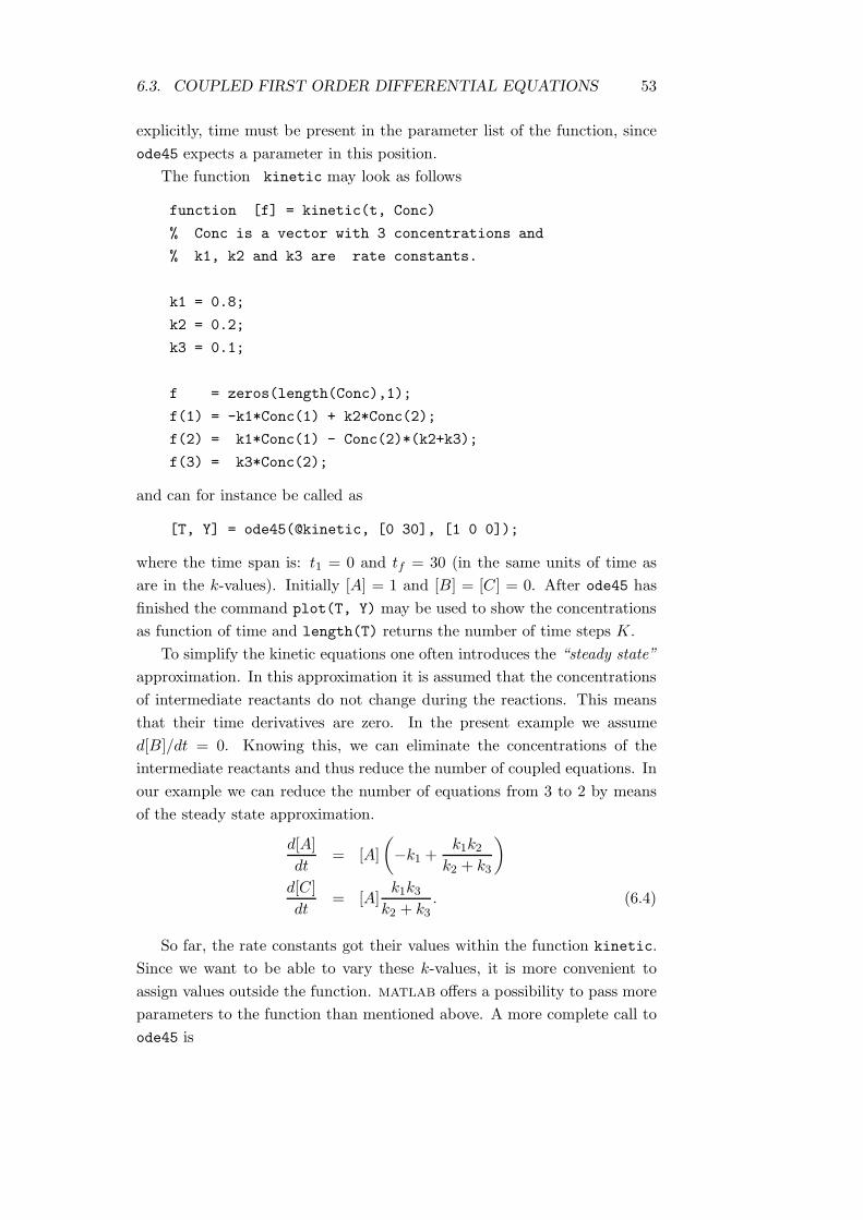
6.3. COUPLED FIRST ORDER DIFFERENTIAL EQUATIONS 53
explicitly, time must be present in the parameter list of the function, since
ode45 expects a parameter in this position.
The function kinetic may look as follows
function [f] = kinetic(t, Conc)
% Conc is a vector with 3 concentrations and
% k1, k2 and k3 are rate constants.
k1 = 0.8;
k2 = 0.2;
k3 = 0.1;
f = zeros(length(Conc),1);
f(1) = -k1*Conc(1) + k2*Conc(2);
f(2) = k1*Conc(1) - Conc(2)*(k2+k3);
f(3) = k3*Conc(2);
and can for instance be called as
[T, Y] = ode45(@kinetic, [0 30], [1 0 0]);
where the time span is: t1 = 0 and tf = 30 (in the same units of time as
are in the k-values). Initially [A] = 1 and [B] = [C] = 0. After ode45 has
finished the command plot(T, Y) may be used to show the concentrations
as function of time and length(T) returns the number of time steps K.
To simplify the kinetic equations one often introduces the “steady state”
approximation. In this approximation it is assumed that the concentrations
of intermediate reactants do not change during the reactions. This means
that their time derivatives are zero. In the present example we assume
d[B]/dt = 0. Knowing this, we can eliminate the concentrations of the
intermediate reactants and thus reduce the number of coupled equations. In
our example we can reduce the number of equations from 3 to 2 by means
of the steady state approximation.
d[A]
dt= [A]
(
−k1 +k1k2
k2 + k3
)
d[C]
dt= [A]
k1k3k2 + k3
. (6.4)
So far, the rate constants got their values within the function kinetic.
Since we want to be able to vary these k-values, it is more convenient to
assign values outside the function. matlab offers a possibility to pass more
parameters to the function than mentioned above. A more complete call to
ode45 is
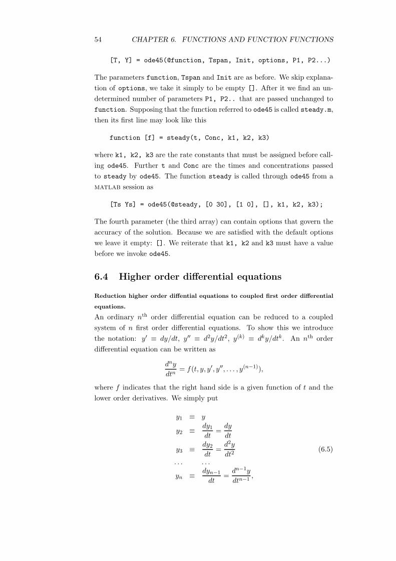
54 CHAPTER 6. FUNCTIONS AND FUNCTION FUNCTIONS
[T, Y] = ode45(@function, Tspan, Init, options, P1, P2...)
The parameters function, Tspan and Init are as before. We skip explana-
tion of options, we take it simply to be empty []. After it we find an un-
determined number of parameters P1, P2.. that are passed unchanged to
function. Supposing that the function referred to ode45 is called steady.m,
then its first line may look like this
function [f] = steady(t, Conc, k1, k2, k3)
where k1, k2, k3 are the rate constants that must be assigned before call-
ing ode45. Further t and Conc are the times and concentrations passed
to steady by ode45. The function steady is called through ode45 from a
matlab session as
[Ts Ys] = ode45(@steady, [0 30], [1 0], [], k1, k2, k3);
The fourth parameter (the third array) can contain options that govern the
accuracy of the solution. Because we are satisfied with the default options
we leave it empty: []. We reiterate that k1, k2 and k3 must have a value
before we invoke ode45.
6.4 Higher order differential equations
Reduction higher order diffential equations to coupled first order differential
equations.
An ordinary nth order differential equation can be reduced to a coupled
system of n first order differential equations. To show this we introduce
the notation: y′ ≡ dy/dt, y′′ ≡ d2y/dt2, y(k) ≡ dky/dtk. An nth order
differential equation can be written as
dny
dtn= f(t, y, y′, y′′, . . . , y(n−1)),
where f indicates that the right hand side is a given function of t and the
lower order derivatives. We simply put
y1 ≡ y
y2 ≡ dy1dt
=dy
dt
y3 ≡ dy2dt
=d2y
dt2(6.5)
. . . . . .
yn ≡ dyn−1
dt=
dn−1y
dtn−1,

6.5. EXERCISES 55
and get the set of n first order coupled equations
dy1dt
= y2
dy2dt
= y3 (6.6)
. . . . . .dyn−1
dt= yn−2
dyndt
≡ dny
dtn= f(t, y, y′, y′′, . . . , y(n−1))
= f(t, y1, y2, y3, . . . , yn).
Example
d2y
dt2= t
dy
dt− y2 (6.7)
becomes
f1 ≡dy1dt
= y2 (6.8)
f2 ≡dy2dt
= ty2 − y21 . (6.9)
In matlab the corresponding function called by the ode solvers would look
like:
function [f] = difeq(t, y)
f = zeros(2,1); % Tell matlab we return a column vector
f(1) = y(2);
f(2) = t*y(2) - y(1)^2;
6.5 Exercises
Exercise 31.
A classic test example for multidimensional minimization is the Rosenbrock
banana function f(x, y) = 100(y − x2)2 + (1− x)2.
1. Write the matlab function banana that evaluates f for the vector
r = (x, y).
2. Call ‘by hand’ fminsearch from your matlab session to minimize the
banana function. Use as a start r = (−1.2, 1).
3. Modify function banana to f(x, y) = 100(y − x2)2 + (a− x)2 and let a
be an input parameter. Read the help of fminsearch to discover how
to pass a to banana via fminsearch.
56 CHAPTER 6. FUNCTIONS AND FUNCTION FUNCTIONS
Exercise 32.
Compute the integral
∫ 1
0
[1
(x− 0.3)2 + 0.01+
1
(x− 0.9)2 + 0.04− 6
]
dx
with the command quad (see helpfile).
Exercise 33.
Write the function
function [r, theta, phi] = cartpol(x)
that returns spherical polar coordinates from the 3-dimensional column
vector x that contains Cartesian coordinates. Remember the equations
(0 ≤ r < ∞, 0 ≤ θ ≤ π, 0 ≤ φ < 2π)
x1x2x3
=
r sin θ cosφr sin θ sinφ
r cos θ
Hints:
• Check first if r = |r| < 10ǫ. If this is the case then set all output pa-
rameters equal to zero and return (with matlab command return).
The constant eps (floating point relative accuracy) is built into mat-
lab; it is 2−52 ≈ 10−16.
• Then test if x21 + x22 ≤ 10ǫ. If this is the case the vector is along the
third axis and φ = 0; it can be pointing up (θ = 0) or pointing down
(θ = 180).
• Finally compute θ from x3 and φ from x1 and notice that φ = arccos y
gives results in the interval 0 ≤ φ ≤ π. If x2 < 0 then φ = 2π − φ.
Exercise 34.
In this exercise we will investigate the steady state approximation by looking
at the increase of concentration of reactant C, see Eq. (6.2). In a reasonable
approximation [C] increases as
[C] = 1− exp(−keff t), (6.10)
where keff is an effective rate constant. By fitting a straight line through
ln(1− [C]) as function of time t we can obtain keff .

6.5. EXERCISES 57
1. Write the .m-files that can be used for the integration of the exact
(6.3) and the steady state equations (6.4).
2. Write a function based on Eq. (6.10) that returns keff .
3. Write a script that first solves the exact equations [by calling the func-
tion you wrote under (1)], then determines keff , and finally solves the
steady state equations and again returns keff . Repeat this for k1 = 0.5,
k2 = 0.5 and k3 = 100k1, 10k1, k1, k1/10, k1/100. Take as initial con-
ditions [A] = 1, [B] = 0 and [C] = 0.
Hint: Do not integrate too long (take tf not too large), a reasonable
upper limit is
tmax= 3/min([k1 k2 k3])
You will see that the steady state approximation is good when B
vanishes quickly, that is if k3 ≫ k1 ≈ k2.
In the case that k3 ≪ k1 ≈ k2 the steady state approximation yields a
keff which is twice too large.
Exercise 35.
Solve Eq. (6.7) by ode45 with initial conditions y1(0) = 1 and y2(0) = 0.
Integrate from t = 0 to t = 0.2. Plot the resulting function y(t) ≡ y1(t).
Exercise 36.
For this exercise we immerse a one-dimensional spring, with a point mass
m attached to it, into a vessel containing a viscous liquid, e.g., syrup. We
pull the spring away from equilibrium over a distance y = 1. At the point
t = 0 we let the spring go, so at this point in time the velocity of m is zero:
dy(0)/dt = 0. The spring will start to vibrate following Newton’s equation
of motion: md2y/dt2 = F . The forces acting on the mass are Hooke’s law:
−ky and the friction force: −fdy/dt (proportional to the velocity). In total,
this so-called “damped harmonic oscillator” satisfies the equation of motion1
md2y
dt2= −ky − f
dy
dt
ord2y
dt2+ ω2y + 2b
dy
dt= 0, (6.11)
where ω =√
k/m and b = f/2m.
1The reader may wonder why somebody in his right mind would put a spring intoa bowl of syrup. However, the damped harmonic oscillator is a useful model in manybranches of science: LCR electric circuits, dispersion of light, etc.

58 CHAPTER 6. FUNCTIONS AND FUNCTION FUNCTIONS
1. Write a function for solving Eq. (6.11), which has, besides t and y,
also b and ω as parameters.
2. Solve this equation by means of ode45 with ω = 1 and b = 0.2.
Integrate over the time span [0, 20]. Take as initial conditions y(0) = 1
and dy(0)/dt = 0.
3. The analytic solution of Eq. (6.11) for b < ω is, with Ω ≡ ω2 − b2,
y = y(0)e−bt
(
cos Ωt+b
ΩsinΩt
)
. (6.12)
Write a script that (i) numerically integrates Eq. (6.11), (ii) imple-
ments the analytic solution, Eq. (6.12), and (iii) shows both solutions
in one plot.
7. More plotting
7.1 3D plots
3D plots and contours
So far we only made two-dimensional plots—values of y against x. We will
now turn to displaying 3D data, i.e., z = f(x, y) will be plotted against x
and y. Of course, we must discretize the function parameters and value. Let
x = (x1, . . . , xm) and y = (y1, . . . , yn) be vectors and let Z be a matrix of
function values
Zij = f(xj, yi).
Note that x carries the column index j of the n × m matrix Z and y the
row index i. The reason is that the x-axis is usually horizontal (corresponds
to running within rows of Z) and the y-axis is usually vertical (runs within
columns of Z).
A matlab function that is useful in the computation of Z is meshgrid.
The statement
[X,Y] = meshgrid(x,y)
transforms vectors (one-dimensional arrays) x and y into two-dimensional
arrays X and Y that can be used with dot operations to compute Z. The rows
of the output array X are simply copies of the vector x and the columns of
the output array Y are copies of the vector y. The number of rows of x
contained in X is the length n of y and the number of columns of Y is equal
to the length m of x. Example:
>> x=[1 2 3 4]; y=[5 4 3];
>> [X Y] = meshgrid(x,y)
X =
1 2 3 4
1 2 3 4
1 2 3 4
Y =
5 5 5 5
4 4 4 4
3 3 3 3
59
60 CHAPTER 7. MORE PLOTTING
That is, Xi,j = xj (independent of i) and Yi,j = yi (independent of j). The
two matrices X and Y created by meshgrid are of the same shape and can
be combined with dot operations, such as .* or ./.
As an example of the use of meshgrid, we evaluate the function
z = f(x, y) = x exp(−x2 − y2)
on an x grid over the range −2 < x < 2 and a y grid with −2 < y < 2.
>> x = -2:0.2:2; y = -2:0.2:2;
>> [X,Y] = meshgrid(x, y);
>> Z = X .* exp(-X.^2 - Y.^2); % Dot operations everywhere
Now
Zi,j ≡ Xi,j exp(−X2i,j − Y 2
i,j) = xj exp(−x2j − y2i ) = f(xj, yi).
The commands mesh(X,Y,Z) and surf(X,Y,Z) give 3D plots on the
screen, while the command contour(X,Y,Z) gives the very same informa-
tion as a contour plot. For presentations the output of surf is the most
spectacular, but for obtaining quantitative information a contour plot is
generally more useful. The difference between mesh and surf is that the
former gives a colored wire frame, while the latter gives a faceted view of
the surface.
We just saw that the first three parameters of the 3D plotting com-
mands: contour, mesh, and surf were two-dimensional matrices, all of the
same dimension. By use of meshgrid we created two such matrices from
two vectors. However, this is not necessary, the first two parameters of the
3D plotting commands may as well be vectors. Obviously, the third pa-
rameter Z, containing the function values Zij = f(xj, yi), must be a n ×m
matrix with its column index j corresponding to x values and its row index
i corresponding to y values.
When the first two parameters, x and y, are vectors, their dimensions
must agree with those of the third parameter Z. That is, if Z is an n × m
matrix, then x must be of dimension m and y must be of dimension n. It is
useful that the 3D plotting commands of matlab can accept vectors when
one wants to plot data generated outside matlab (by another program or
by measurements as, for instance, 2D nmr). In such a case you usually
have at your disposal a vector of x values, a vector of y values and a matrix
of function values that correspond to these vectors. There is then no need
to blow up the vectors x and y to matrices, which we did by the use of
meshgrid.

7.2. HANDLE GRAPHICS 61
7.2 Handle Graphics
Graphical hierarchy
matlab has a system, called Handle Graphics, by which you can directly
manipulate graphics elements. This system offers unlimited possibilities
to create and modify all types of graphs. The organization of a graph is
hierarchical and object oriented. At the top is the Root, which simply is
your matlab screen. This object is created when you start up matlab.
Figure objects are the individual windows on the Root screen, they are
referred to as the children of the Root. There is no limit on the number of
Figures. A Figure object is created automatically by the commands that
we introduced earlier, namely plot, mesh, contour and surf. As for all
graphical objects, there is also a separate low level command that creates
the object: figure creates a new Figure as a child of Root. If there are
multiple Figures within the Root, one Figure is always designated as the
“current” figure; all subsequent graphics commands, such as xlabel will
give output to this figure.
Figure 7.1: Graphics Hierarchy Tree
A Figure object has as children the objects Axes, which define regions
in a Figure window. All commands such as plot automatically create an
Axes object if it does not exist. Only one Axes object can be current. The
children of Axes are Image, Line, Patch, Surface, and Text. Image consists
of pixels; see the matlab on-line documentation for more details. The
Line object is the basic graphic primitive used for most 2D and 3D plots.
High level functions such as plot and contour create these objects. The
coordinate system of the parent Axes positions the Line object in the plot.

62 CHAPTER 7. MORE PLOTTING
Patch objects are filled polygons and are created by high level commands
such as bar, which creates a bar graph. Surface objects represent 3D data
and are created by mesh and surf.
The final objects are Text, which are also children of Axes. Text objects
are character strings and are created by high level commands such as xlabel,
ylabel and title, which we met earlier.
7.3 Handles of graphical objects
Handles and a few low level graphical commands.
Every individual graphics object has a unique identifier, called a handle, that
matlab assigns to it when the object is created. By using these handles as
variables we can manipulate very easily all objects in a plot. As an example
we return to contour. Thus far we plotted contours without numbers, which
is not particularly useful. However, the matlab command contour can
return values associated with each contour line. Moreover the command
returns the handle of every contour line. Example:
>> x = linspace(-1,1,20); % 20 equidistant points
>> y = linspace(-2,2,40);
>> [X Y] = meshgrid(x,y);
>> Z = Y.^2.*exp(-X.^2-Y.^2);
>> [c h] = contour(X,Y,Z,10); % 10 levels
>> whos c h
Name Size Bytes Class
c 2x892 14272 double array
h 32x1 256 double array
matlab interpolates the z values by means of an unspecified algorithm.
Furthermore, the length of c, containing contour values, is unpredictable,
as is the length of h. One would perhaps expect the vector of handles h to
be of length 20 (10 levels are requested of a two-fold symmetric function).
However, lines cut by borders become separate graphical objects and there-
fore h is longer than 20 (in the example 32). The important use of the arrays
c and h is in the command clabel. This command draws the labels in the
contour plot. Continuing the example, the command
>> clabel(c,h)
draws labels in the current figure (which must be drawn by contour). Doing
this, one gets a crowded plot, the labels are often too close to each other. The
command clabel(c,h,’manual’) offers the possibility to pick the positions
interactively.

7.3. HANDLES OF GRAPHICAL OBJECTS 63
As another example of the use of handles, we consider the command
plot. When we issue h=plot(x,Y), where Y is a matrix, then of course
the plots appear, but in addition the vector h will appear on the screen.
Its elements contain unique identification numbers of the curves: the line
handles. Each curve in the figure corresponds to an element of the vector h.
These line handles allow us to make modifications to the individual curves.
(Obviously, h is only of length > 1 if we plot more than one curve with the
same plot statement. If we plot two curves one after the other by issuing
the plot command twice and the toggle hold in the on state, then we get
twice a different scalar back as the line handle.)
As an example of the use of a line handle, we first plot two straight lines
and then change the color of the second to red, which by default was drawn
by matlab in faint green.
>> h = plot([1:10]’, [[1:10]’ [2:11]’]) % no semicolon
h =
103.0029 % these are the handles
3.0063 % usually they are floating point numbers
>> set(h(2), ’color’, ’red’) % second line red
The low level command set acts on the line with line handle h(2) and
changes the color of this line to red. Note that set does not erase the plot
and does not start a new one, it acts on the existing (current) plot. High
level commands, such as plot, contour, etc., do start a new plot (unless
the hold status is on).
Line handles can also be used to get information about the graphical
object.
>> set(h(2)) % Inspect possible settings of second curve
Color
EraseMode: [ normal | background | xor | none ]
LineStyle: [ - | -- | : | -. | none ]
....
>> get(h(2)) % Inspect actual settings of second curve
Color = [1 0 0]
EraseMode = normal
LineStyle = -
....
The command set(h(2)) returns the possible settings for the second curve,
the command get(h(2)) returns the actual choices. We see that “color” is
a property of object Line, and that the actual choice of color is given by the
array [1 0 0].

64 CHAPTER 7. MORE PLOTTING
In the “rgb” color scheme used here, this implies that the color chosen is
pure red, as is expected because we changed the line color to red. (The array
[1 0 1] would give an equal mixture of red and blue, which is magenta).
We see the possible line styles (see help plot) and the actual choice: solid
(the default).
Suppose now we want change the line style of the second curve to dotted.
We see that linestyle (not case sensitive!) is a property of object with
handle h(2). We can change it with set(h(2), ’linest’, ’:’). This
turns it into a dotted line. Note that unique abbreviations (linest instead
of linestyle) of the property names of the objects are allowed.
As we said, all objects have a handle, also the Axes objects in a Figure
object; by gca (“get current axes”) we get the handle of the current Axes
in the current Figure and by get(gca) we get the actual values of the
properties of this Axes object. We see that one of the Axes properties is
FontSize. If we want to increase to 20 points the size of the digits on the
axes, we issue set(gca, ’Fontsize’, 20).
Fortunately, it is often not necessary to use these low level commands,
matlab has several high level commands that make life easier. For instance
the aspect ratio (ratio between x-axis and y-axis scale) can be set by a
command of the type set(gca,’DataAspectRatio’,[1 1 1]). However,
much easier is the use of the high level function axis; see its help.
By left clicking with the mouse on an object we turn it into the “current
object”. Its handle is returned by the command gco (“get current object”).
So, if we want to change the color of a line on the screen to blue and we
forgot to save its handle, then we can click on it and issue the command
set(gco, ’col’, ’b’).
Remove an object by using the function delete, passing the object’s
handle as the argument. For example, delete the current Axes (and all of
its children!) by delete(gca).
We can draw lines in the coordinate system of the current Axes object
by the low level command
line([x1 x2 .. xn], [y1 y2 .. yn])
This draws a line from point (x1, y1) to point (x2, y2), etc., to point (xn, yn).
But first we want to give the plot a definite size by
axis([xmin xmax ymin ymax])
which defines an x-axis from xmin to xmax and a y-axis from ymin to ymax.
For example, the following code draws a rectangular box:
7.4. POLAR PLOTS 65
>> close all % close all existing figures
>> axis([0 10 0 20])
>> h = line([2 5 5 2 2], [2 2 4 4 2])
We define first an x-axis from 0 to 10 and a y axis from 0 to 20. If we do
not do this, the axes are generated by the line command and the boundaries
of the box will coincide with the axes, which is usually not what you want.
The line command draws lines from the successive points (2, 2) to (5, 2) to
(5, 4) to (2, 4) back to (2, 2). This is a rectangular box with width 3 and
height 2 with the lower left hand corner at the point (2, 2).
We can place text in the plot by the command text(x,y,’text’). For
instance in the box that we just drew, beginning at point (2.5, 3):
>> t = text(2.5, 3, ’ Text ’, ’fontsize’, 20, ...
’fontname’, ’arial black’)
Note that the fontsize has a different unit of size than the axes. Arial black
is the name of a font; matlab can handle different fonts, enter listfonts
to see which ones are available.
7.4 Polar plots
2D and 3D polar plots
Atomic orbitals pervade all of chemistry. Invariably they are drawn as 3D
polar plots and therefore we will show how matlab can visualize 3D polar
plots. Of course, orbitals may also be drawn as contour diagrams, which is
commonly done for molecular orbitals.
Atomic orbitals are products of the form f(r) g(θ, φ), where we meet
again spherical polar coordinates defined by
xyz
=
r sin θ cosφr sin θ sinφ
r cos θ
, 0 ≤ r < ∞, 0 ≤ θ ≤ π, 0 ≤ φ < 2π. (7.1)
In polar plots one draws only the angular part g(θ, φ), taking a fixed radial
part f(r0).
matlab is able to make 2D polar plots, but not 3D polar plots, so we
must do this ourselves. Let us first explain how to make a 2D polar plot
by hand. Say, we want to plot the angular part of the function f(r)g(φ).
Figure 7.2 shows polar graph paper that helps us do this. We choose a
fixed value r0 and mark points for φ = 0, 20, · · · , 340 with the value
of h(φi) ≡ |f(r0)g(φi)| as the distance from the origin. The equidistant
circles help us in measuring this distance. In other words, we mark points

66 CHAPTER 7. MORE PLOTTING
0°
20°
40°
60°
80°100°
120°
140°
160°
180°
200°
220°
240°
260° 280°
300°
320°
340°
Figure 7.2: Polar plot paper
(xi, yi) = (r cosφi, r sinφi), but substitute for r the positive function values
h(φi). After marking the points we draw a line through the points.
As an example, we make a polar plot of g(φ) = cosφ [f(r0) = 1] and
since the computer does the work, we take a much finer grid than we would
do by hand.
phi = [0:1:360]*pi/180;
x = cos(phi);
y = sin(phi);
h = abs(cos(phi));
plot( h.*x, h.*y)
axis equal
The generalization to 3D is clear now. For instance, if we want to plot
the 2pz atomic orbital r exp(−r) cos θ, we choose a constant value r0 for r,
but since the factor r0 exp(−r0) does not affect the shape of the plot, we
ignore it. We write g(θ, φ) = cos θ, h(θ) = |g(θ)| and plot z = cos θ against
x = h(φ) sin θ cosφ and y = h(φ) sin θ sinφ. In matlab:
theta = [0:5:180]*pi/180;
phi = [0:5:360]*pi/180;
[Theta, Phi] = meshgrid(theta, phi);

7.5. EXERCISES 67
H = abs(cos(Theta));
X = H.*sin(Theta).*cos(Phi);
Y = H.*sin(Theta).*sin(Phi);
Z = H.*cos(Theta);
surf(X,Y,Z)
axis equal off
The same can be achieved in a slightly more efficient manner
theta = [0:5:180]*pi/180;
phi = [0:5:360]*pi/180;
h = abs(cos(theta));
X = cos(phi’)*sin(theta)*diag(h);
Y = sin(phi’)*sin(theta)*diag(h);
Z = repmat(cos(theta), length(phi),1)*diag(h);
surf(X,Y,Z)
axis equal off
Here X and Y are obtained from column vector times row vector multiplica-
tion (dyadic product).
7.5 Exercises
Exercise 37.
Write a script (or function) that, by using meshgrid, draws the “Mexican
hat”
z = (1− x2 − y2) exp(−0.5(x2 + y2))
on the x and y interval [−3, 3]. Do not use any for loops. Apply one after
the other: mesh, surf, and contour. Use matrices for all parameters.
Hint:
Between the plot commands you may enter in your script the matlab com-
mand pause. This allows you to have a look at the plot until you hit the
enter key.
Exercise 38.
Return to the previous exercise, change your script (or function) so that
the first two parameters of contour, mesh, and surf are the vectors that
were used in the meshgrid command. Verify that the figures are exactly
the same as when the first two parameters were the two matrices created by
meshgrid.
Exercise 39.

68 CHAPTER 7. MORE PLOTTING
The so-called “sinc” function is defined as follows
sinc(r) =
sin(πr)
πrif r 6= 0
1 if r = 0.
The matlab function sinc can be called with any matrix as input. Use
this function to plot sinc(x2+ y2) on the grid [−3, 3] for both x and y. First
look at the result of surf and use the rotate button to admire the function
from all sides. Then use the contour and clabel command to put manually
values on the contours.
Exercise 40.
Draw the naphthalene molecule as in Fig. 7.3.
Figure 7.3: Standard numbering of the naphthalene molecule
7
8
9
1
2
3
4
10
5
6
Hints: Build a 2×10 matrix R that contains the coordinates of the carbon
atoms.
• Choose (0, 1) as coordinates of atom 1 and obtain coordinates of atom
2, 3, 4, 10, and 9 by consecutive rotations over 60.
• Translate the 6 ring thus obtained to the left: xi 7→ xi − x10.
• Get atoms 5, 6, 7, and 8 by reflection, x8 = −x1 and y8 = y1, etc.
Then put all x-coordinates of points to be connected in a single array and
do the same for the y-coordinates. Determine the size of your plot by axis
and use line to do the actual drawing.
The numbers can be written by text(x,y,’s’). This can be done ‘by
hand’, or more elegantly in a loop over the atoms. Use the command
num2str to convert n to a string (quotes must then not be used in the
command text).

7.5. EXERCISES 69
Exercise 41.
A normalized hydrogen 3dz2 orbital has the form
N r2 e−ζr (3z2 − r2) with r =√
x2 + y2 + z2 and N =1
3
√
1
2πζ7/2.
Write a script that plots the intersection of this orbital with the yz-plane,
that is, for x = 0. Choose ζ = 3, and let y and z range from −4 to +4.
Hint:
Use for contouring something like
[c h]=contour(Y, Z, dorb, [-1:0.05:1]);
clabel(c,h, ’fontsize’,6.5)
where dorb must contain the values of the 3dz2 orbital on the y-z grid, the
array [-1:0.05:1] gives the contour levels and the second statement puts
labels on the contours.
Exercise 42.
• Plot the d-orbital of the previous exercise in polar form. Here you
may forget about the normalization constant, because only the shape
matters, not the values.
• Plot 2p2x = r2 exp(−2r) sin2 θ cos2 φ (unnormalized) in polar form. Do
not forget the aspect ratio axis equal! Do you recognize this plot?

70 CHAPTER 7. MORE PLOTTING
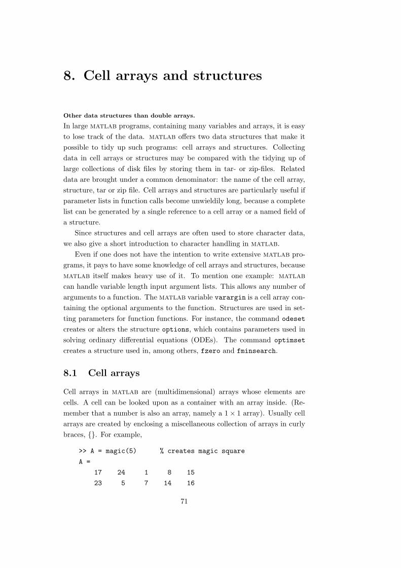
8. Cell arrays and structures
Other data structures than double arrays.
In large matlab programs, containing many variables and arrays, it is easy
to lose track of the data. matlab offers two data structures that make it
possible to tidy up such programs: cell arrays and structures. Collecting
data in cell arrays or structures may be compared with the tidying up of
large collections of disk files by storing them in tar- or zip-files. Related
data are brought under a common denominator: the name of the cell array,
structure, tar or zip file. Cell arrays and structures are particularly useful if
parameter lists in function calls become unwieldily long, because a complete
list can be generated by a single reference to a cell array or a named field of
a structure.
Since structures and cell arrays are often used to store character data,
we also give a short introduction to character handling in matlab.
Even if one does not have the intention to write extensive matlab pro-
grams, it pays to have some knowledge of cell arrays and structures, because
matlab itself makes heavy use of it. To mention one example: matlab
can handle variable length input argument lists. This allows any number of
arguments to a function. The matlab variable varargin is a cell array con-
taining the optional arguments to the function. Structures are used in set-
ting parameters for function functions. For instance, the command odeset
creates or alters the structure options, which contains parameters used in
solving ordinary differential equations (ODEs). The command optimset
creates a structure used in, among others, fzero and fminsearch.
8.1 Cell arrays
Cell arrays in matlab are (multidimensional) arrays whose elements are
cells. A cell can be looked upon as a container with an array inside. (Re-
member that a number is also an array, namely a 1× 1 array). Usually cell
arrays are created by enclosing a miscellaneous collection of arrays in curly
braces, . For example,
>> A = magic(5) % creates magic square
A =
17 24 1 8 15
23 5 7 14 16
71

72 CHAPTER 8. CELL ARRAYS AND STRUCTURES
4 6 13 20 22
10 12 19 21 3
11 18 25 2 9
>> C = A sum(A) prod(prod(A)) % creates cell array
C =
[5x5 double] [1x5 double] [1.5511e+025]
These two commands produce (i) the magic square matrix A (all rows and
columns sum to 65, elements are 1, 2, . . . , 25) and (ii) the 1× 3 cell array C.
The function prod takes the products of elements in the columns of A and
returns a row vector. The second prod takes the product of the elements
in this row vector. The three cells of cell array C contain now the following
arrays, which are of different dimension:
• the square matrix A in C(1,1),
• the row vector of column sums in C(1,2),
• the product of all its elements in C(1,3).
The contents of the cells in cell array C are not fully displayed because the
first two cells are too large to print in this limited space, but the third cell
contains only a single number, 25!, so there is room to print it.
Here are two important points to remember. First, to retrieve the cell
itself (container plus content) use round brackets. Since a cell is nothing but
a 1×1 cell array, matlab command whos tells us that e.g. C(1,2) retrieves
a cell array. Second to retrieve the content of the cell use subscripts in curly
braces. For example, C3, or equivalently C1,3, retrieves 25!, whereas
C(3) retrieves the third cell. Notice the difference (C is the cell array of
previous example):
>> c=C(1) % Get cell (1-by-1 cell array)
c =
[5x5 double]
>> whos c
Name Size Bytes Class
c 1x1 260 cell array
>> d=C1 % Get content of cell (5-by-5 magic square)
d =
17 24 1 8 15
23 5 7 14 16
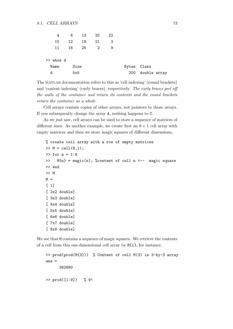
8.1. CELL ARRAYS 73
4 6 13 20 22
10 12 19 21 3
11 18 25 2 9
>> whos d
Name Size Bytes Class
d 5x5 200 double array
The matlab documentation refers to this as ‘cell indexing’ (round brackets)
and ‘content indexing’ (curly braces), respectively. The curly braces peel off
the walls of the container and return its contents and the round brackets
return the container as a whole.
Cell arrays contain copies of other arrays, not pointers to those arrays.
If you subsequently change the array A, nothing happens to C.
As we just saw, cell arrays can be used to store a sequence of matrices of
different sizes. As another example, we create first an 8× 1 cell array with
empty matrices and then we store magic squares of different dimensions,
% create cell array with a row of empty matrices
>> M = cell(8,1);
>> for n = 1:8
>> Mn = magic(n); %content of cell n <-- magic square
>> end
>> M
M =
[ 1]
[ 2x2 double]
[ 3x3 double]
[ 4x4 double]
[ 5x5 double]
[ 6x6 double]
[ 7x7 double]
[ 8x8 double]
We see that M contains a sequence of magic squares. We retrieve the contents
of a cell from this one-dimensional cell array by Mi, for instance,
>> prod(prod(M3)) % Content of cell M(3) is 3-by-3 array
ans =
362880
>> prod([1:9]) % 9!

74 CHAPTER 8. CELL ARRAYS AND STRUCTURES
ans =
362880
Using round brackets, as in prod(M(3)), we get an error message because
the function prod cannot take the product of a cell, only the contents of the
cell can be multiplied.
As we saw above, a set of curly brackets around a set of one or more
arrays converts the set into a cell array. So, in the example above we could
as well have written M(n)=magic(n) instead of Mn=magic(n). The first
form creates on the right hand side a cell containing a magic square and
assigns this cell to the nth cell of M. The second form adds the magic square
to the content of the nth cell of M
Only cells may be assigned to cells:
>> a = cell(2);
>> a(1) = [1 2 3] % Wrong, rhs is not a cell
??? Conversion to cell from double is not possible.
>> a(1) = [1 2 3] % OK, rhs is a cell
a =
[1x3 double]
>> b = cell(2,2);
>> b(1,2) = a(1) % cell a(1) assigned to cell b(1,2)
% Content of cell a(1) to content of cell b(1,2):
>> b1,2 = a1
When you use a range of cells in curly brackets, as in Ai:j, the contents
of the cells are listed one after the other separated by commas. In a situation
where matlab expects such a comma separated list this is OK. For instance,
>> A1 = [1 2];
>> A2 = [3 4 5];
>> A3 = [6 7 8 9 10];
>> % Comma separated list between square brackets
>> [A1:3]
>> % identical to:
>> [1, 2, 3, 4, 5, 6, 7, 8, 9, 10]
To assign more than one element of a cell array to another, do not use
curly brackets on the left hand side, because in general a comma separated
list is not allowed on the left hand side of an assignment. Example:
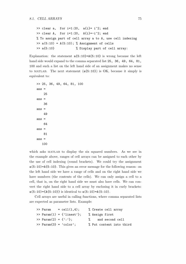
8.1. CELL ARRAYS 75
>> clear a, for i=1:20, ai= i^2; end
>> clear A, for i=1:20, Ai=-i^2; end
% To assign part of cell array a to A, use cell indexing
>> a(5:10) = A(5:10); % Assignment of cells
>> a5:10 % Display part of cell array:
Explanation: the statement a5:10=A5:10 is wrong because the left
hand side would expand to the comma separated list 25, 36, 49, 64, 81,
100 and such a list on the left hand side of an assignment makes no sense
to matlab. The next statement (a5:10) is OK, because it simply is
equivalent to:
>> 25, 36, 49, 64, 81, 100
ans =
25
ans =
36
ans =
49
ans =
64
ans =
81
ans =
100
which asks matlab to display the six squared numbers. As we see in
the example above, ranges of cell arrays can be assigned to each other by
the use of cell indexing (round brackets). We could try the assignment
a(5:10)=A5:10. This gives an error message for the following reason: on
the left hand side we have a range of cells and on the right hand side we
have numbers (the contents of the cells). We can only assign a cell to a
cell, that is, on the right hand side we must also have cells. We can con-
vert the right hand side to a cell array by enclosing it in curly brackets:
a(5:10)=A5:10 is identical to a(5:10)=A(5:10).
Cell arrays are useful in calling functions, where comma separated lists
are expected as parameter lists. Example:
>> Param = cell(1,4); % Create cell array
>> Param(1) = ’linest’; % Assign first
>> Param(2) = ’:’; % and second cell
>> Param3 = ’color’; % Put content into third

76 CHAPTER 8. CELL ARRAYS AND STRUCTURES
>> Param4 = ’red’; % and fourth cell
>> plot(sin(0:pi/10:2*pi), Param:)
Here Param: expands to a comma separated list, i.e., the four parameters
are passed (separated by commas) to plot.
In summary, a cell array is a matlab array for which the elements are
cells, containers that hold other matlab arrays. For example, one cell of a
cell array might contain a real matrix, another an array of text strings, and
another a vector of complex values. You can build cell arrays of any valid
size or shape, including multidimensional structure arrays.
8.2 Characters
We can enter text into matlab by using single quotes. For example,
s = ’Hello’
The result is not the same kind of numeric array as we have been dealing
with up to now. It is a 1× 5 character array, briefly referred to as a string.
Internally matlab stores a letter as a two byte numeric value, not as a
floating point number (8 bytes).
There exists a well-known convention called ascii (American Standard
Code for Information Interchange) to store letters as numbers. In ascii the
uppercase letters A,. . . , Z have code 65, . . . ,90 and the lowercase letters
a,. . . , z have code 97,. . . ,122. The function char converts an ascii code
to an internal matlab code. Conversely, the statement a = double(s)
converts the character array to a numeric matrix a containing the ascii
codes for each character. Example:
>> s = ’hello’;
>> a = double(s)
a =
104 101 108 108 111
>> b = char(a) % array a contains numbers
b =
hello
The result a = 104 101 108 108 111 is the ascii representation of hello.
Concatenation with square brackets joins text variables together into
larger strings. The second statement joins the strings horizontally:
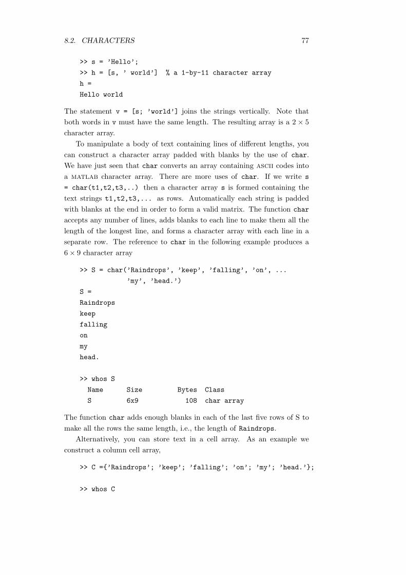
8.2. CHARACTERS 77
>> s = ’Hello’;
>> h = [s, ’ world’] % a 1-by-11 character array
h =
Hello world
The statement v = [s; ’world’] joins the strings vertically. Note that
both words in v must have the same length. The resulting array is a 2 × 5
character array.
To manipulate a body of text containing lines of different lengths, you
can construct a character array padded with blanks by the use of char.
We have just seen that char converts an array containing ascii codes into
a matlab character array. There are more uses of char. If we write s
= char(t1,t2,t3,..) then a character array s is formed containing the
text strings t1,t2,t3,... as rows. Automatically each string is padded
with blanks at the end in order to form a valid matrix. The function char
accepts any number of lines, adds blanks to each line to make them all the
length of the longest line, and forms a character array with each line in a
separate row. The reference to char in the following example produces a
6× 9 character array
>> S = char(’Raindrops’, ’keep’, ’falling’, ’on’, ...
’my’, ’head.’)
S =
Raindrops
keep
falling
on
my
head.
>> whos S
Name Size Bytes Class
S 6x9 108 char array
The function char adds enough blanks in each of the last five rows of S to
make all the rows the same length, i.e., the length of Raindrops.
Alternatively, you can store text in a cell array. As an example we
construct a column cell array,
>> C =’Raindrops’; ’keep’; ’falling’; ’on’; ’my’; ’head.’;
>> whos C

78 CHAPTER 8. CELL ARRAYS AND STRUCTURES
Name Size Bytes Class
C 6x1 610 cell array
The contents of the cells are arrays (in this example character arrays), in
agreement with our definition of a cell array. You can convert a character
array S to a cell array of strings with C = cellstr(S) and reverse the
process with S = char(C:) (comma separated list passed to char).
Generally speaking cell arrays are more flexible than character arrays.
For instance, transposition of the 6× 1 cell array C gives
>> C’ % cell array from the previous example
ans =
’Raindrops’ ’keep’ ’falling’ ’on’ ’my’ ’head.’
which is a 1 × 6 cell array with the same strings as contents of the cells.
Transposition of the 6× 9 character array S on the other hand gives
>> S’ % character array
ans =
Rkfomh
aeanye
iel a
npl d
d i .
r n
o g
p
s
which is generally less useful (unless you are a composer of crosswords).
8.3 Structures
Structures are multidimensional matlab arrays with elements accessed by
designators that are strings. For example, let us build a data base for a
certain course. Each entry contains a student name, student number and
grade,
>> S.name = ’Hans Jansen’;
>> S.number = ’005143’;
>> S.grade = 7.5
creates a scalar structure with three fields:
8.3. STRUCTURES 79
S =
name: ’Hans Jansen’
number: ’005143’
grade: 7.5000
Like everything else in matlab, structures are arrays, so you can insert
additional elements. In this case, each element of the array is a structure
with several fields. The fields can be added one at a time,
>> S(2).name = ’Sandy de Vries’;
>> S(2).number = ’995103’;
>> S(2).grade = 8;
The scalar structure S has now become a 1× 2 array, with S(1) referring to
student Hans Jansen and S(2) to Sandy de Vries.
An entire element can be added with a single statement.
>> S(3) = struct(’name’,’Jerry Zwartwater’,...
’number’,’985099’,’grade’,7)
The structure is large enough that only a summary is printed,
S =
1x3 struct array with fields:
name
number
grade
There are several ways to reassemble the various fields into other matlab
arrays. They are all based on the notion of a comma separated list. We have
already met this notion in the discussion of the cell arrays. Typing
>> S.number
is the same as typing S(1).number, S(2).number, S(3).number. This is
a comma separated list. It assigns the three student numbers, one at a time,
to the default variable ans and displays these numbers. When you enclose
the expression in square brackets, [S.grade] it is the same as [S(1).grade,
S(2).grade, S(3).grade] which produces a row vector containing all of
the grades. The statement
>> mean([S.grade])
ans =
7.5000
80 CHAPTER 8. CELL ARRAYS AND STRUCTURES
gives the average grade of the three students now present in our data base.
Just as in the case of comma separated lists obtained from cell arrays, we
must be careful that we generate the lists only in contexts where matlab
expects such lists. This is in six situations:
• Combination of statements on one line plus output, e.g. >> a,b,c,d
• inside [ ] for horizontal concatenation, e.g. [a,b,c,d]
• inside to create a cell array, e.g. a,b,c,d
• inside ( ) for function input arguments, e.g. test(a,b)
• inside ( ) for array indexing, e.g. A(k,l)
• inside [ ] for multiple function output arguments, e.g. [v,d] = eig(a).
Because of this expansion into a comma separated list, structures can be
easily converted to cell arrays. Enclosing an expression in curly braces, as
for instance S.name, creates a 1×3 cell array containing the three names.
>> S.name
ans =
’Hans Jansen’ ’Sandy de Vries’ ’Jerry Zwartwater’
Since S.name expands to a list containing the contents of the name fields,
this statement is completely equivalent to
ans = ’Hans Jansen’, ’Sandy de Vries’, ’Jerry Zwartwater’
which, as we saw above, creates a cell array with three cells having the three
student names as their contents.
An expansion to a comma separated list is useful as a parameter list in
a function call. Above we gave an example where we passed a parameter
list to plot by expanding the cell array Param. As an example of expanding
a structure, we call char, which, as we saw in subsection 8.2, creates a
character array with the entries padded with blanks, so that all rows are of
equal length:
>> N=char(S.name) % expansion to comma separated list
N =
Hans Jansen
Sandy de Vries
Jerry Zwartwater
>> whos N
Name Size Bytes Class
N 3x16 96 char array
8.3. STRUCTURES 81
In Table 8.1 we list a few matlab functions that can handle text, cell
arrays, and structures.
Table 8.1: Some functions useful for cell array, structure and character han-
dling; see help files for details.
cell Create cell array.cell2struct Convert cell array into structure array.celldisp Display cell array contents.cellfun Apply a cell function to a cell array.cellplot Display graphical depiction of cell array.char Create character array (string).deal Deal inputs to outputsdeblank Remove trailing blanks from a stringfieldnames Get structure field names.findstr Find one string within another.int2str Convert integer to string.iscell True for cell array.isfield True if field is in structure array.isstruct True for structures.num2cell Convert numeric array into cell array.num2str Convert number to string.rmfield Remove structure field.strcat Concatenate stringsstrcmp Compare stringsstrmatch Find possible matches for a stringstruct Create or convert to structure array.struct2cell Convert structure array into cell array.
Cell arrays are useful for organizing data that consist of different sizes or
kinds of data. Cell arrays are better than structures for applications when
you don’t have a fixed set of field names. Furthermore, retrieving data from
a cell array can be done in one statement, whereas retrieving from different
fields of a structure would take more than one statement. As an example of
the latter assertion, assume that your data consist of:
• A 3× 4 array with measured values (real numbers).
• A 15-character string containing the name of the student who per-
formed the measurements.
• The date of the experiment, a 10-character string as ’23-09-2003’.
• A 3 × 4 × 5 array containing a record of measurements taken for the
past 5 experiments.
A good data construct for these data could be a structure. But if you usually
access only the first three fields, then a cell array might be more convenient
for indexing purposes. To access the first three elements of the cell array
TEST use the command deal. The statement
82 CHAPTER 8. CELL ARRAYS AND STRUCTURES
[newdata, name, date] = deal(TEST1:3)
retrieves the contents of the first three cells and assigns them to the array
newdata and the strings name and date, respectively. The function deal is
new. It is a general function that deals inputs to outputs:
[a,b,c,...] = deal(x,y,z,...)
simply matches up the input and output lists. It is the same as a=x, b=y,
c=z,. . . . The only way to assign multiple values to a left hand side is by
means of a function call. This is the reason of the existence of the function
deal. On the other hand, to access different fields of the structure test, we
need three statements:
newdata = test.measure
name = test.name
date = test.date
8.4 Exercises
Exercise 43.
1. Type in
t = ’oranges are grown in the tropics’
Read the help of findstr. Parse this string into words by the aid of
the output of findstr. That is, get six strings (character arrays) that
contain the respective words. Store these strings in a cell array. Make
sure that you do not have beginning or trailing blanks in the words.
2. Write a function parse that parses general strings.
Hints:
Check the input of the function by ischar. Make sure that the input
string does not have trailing blanks by the use of deblank.
Exercise 44.
Write a script that writes names and sizes of files in the current directory to
the screen. Each line must show the filename followed by its size (in bytes).
Show the files sorted with respect to size.
Hints:
1. The command dir returns a structure with the current filenames and
sizes.

8.4. EXERCISES 83
2. The command sort can return the sorted array together with the
permutation that achieves the actual sorting.
3. matlab does not echo properly an array of the kind [char num].
Apply int2str to num to get readable output.
Exercise 45.
Predict—without executing the following script—what it will put on your
screen:
clear all;
a = magic(3);
b = ’a’ ’b’ ’c’
’d’ ’e’ ’f’;
c(1,1).income = 22000;
c(2,4).age = 24;
d = rand(4,7);
e = a b ...
c d ;
u = size(e);
k = 0;
for i=1:u(1)
for j=1:u(2)
k = k+1;
siz(k,:) = [size(ei,j)];
end
end
siz = [siz; u]
clear u i j k siz
A = whos;
for i=1:length(A)
siz(i,:) = A(i).size;
end
siz
Visit
http:/www.theochem.kun.nl/~pwormer/matlab/ml.html.

84 CHAPTER 8. CELL ARRAYS AND STRUCTURES
where you will find this script under the name size_struct.m. Download
it to your directory and execute it. Was your prediction correct? If not,
experiment with the appropriate matlab statements until you feel that you
understand what is going on in this script (that serves no other purpose
than comparing matlab data structures and their dimensions).
Exercise 46.
Design a matlab data structure for the periodic system of elements. Include
the following information:
• The full English name of the element and its standard chemical ab-
breviation.
• The masses and abundances of the naturally occurring isotopes.
• Electron configuration, i.e., number of electrons in n = 1, 2, . . .. shells.
• Prepare the periodic system for the first 10 elements. A .txt file of
isotopic masses can be found at the url
http:/www.theochem.kun.nl/~pwormer/matlab/ml.html.
The same site contains a periodic system as a .pdf file. This informa-
tion originates from the usa government:
http://physics.nist.gov/PhysRefData/Compositions/index.html