theory, guidance, and flight control for high
TRANSCRIPT

Theory, Guidance, and Flight Control for High
Maneuverability Projectiles
by Frank Fresconi, Ilmars Celmins, and Sidra I. Silton
ARL-TR-6767 January 2014
Approved for public release; distribution is unlimited.

NOTICES
Disclaimers
The findings in this report are not to be construed as an official Department of the Army position unless
so designated by other authorized documents.
Citation of manufacturer’s or trade names does not constitute an official endorsement or approval of the
use thereof.
Destroy this report when it is no longer needed. Do not return it to the originator.
Army Research Laboratory Aberdeen Proving Ground, MD 21005-5066
ARL-TR-6767 January 2014
Theory, Guidance, and Flight Control for High
Maneuverability Projectiles
Frank Fresconi, Ilmars Celmins, and Sidra I. Silton
Weapons and Materials Research Directorate, ARL
Approved for public release; distribution is unlimited.

ii
REPORT DOCUMENTATION PAGE Form Approved OMB No. 0704-0188
Public reporting burden for this collection of information is estimated to average 1 hour per response, including the time for reviewing instructions, searching existing data sources, gathering and maintaining the data needed, and completing and reviewing the collection information. Send comments regarding this burden estimate or any other aspect of this collection of information, including suggestions for reducing the burden, to Department of Defense, Washington Headquarters Services, Directorate for Information Operations and Reports (0704-0188), 1215 Jefferson Davis Highway, Suite 1204, Arlington, VA 22202-4302. Respondents should be aware that notwithstanding any other provision of law, no person shall be subject to any penalty for failing to comply with a collection of information if it does not display a currently valid OMB control number.
PLEASE DO NOT RETURN YOUR FORM TO THE ABOVE ADDRESS.
1. REPORT DATE (DD-MM-YYYY)
January 2014
2. REPORT TYPE
Final
3. DATES COVERED (From - To)
October 2010–June 2013 4. TITLE AND SUBTITLE
Theory, Guidance, and Flight Control for High Maneuverability Projectiles
5a. CONTRACT NUMBER
5b. GRANT NUMBER
5c. PROGRAM ELEMENT NUMBER
6. AUTHOR(S)
Frank Fresconi, Ilmars Celmins, and Sidra I. Silton
5d. PROJECT NUMBER
AH43 5e. TASK NUMBER
5f. WORK UNIT NUMBER
7. PERFORMING ORGANIZATION NAME(S) AND ADDRESS(ES)
U.S. Army Research Laboratory
ATTN: RDRL-WML-E
Aberdeen Proving Ground, MD 21005-5066
8. PERFORMING ORGANIZATION REPORT NUMBER
ARL-TR-6767
9. SPONSORING/MONITORING AGENCY NAME(S) AND ADDRESS(ES)
10. SPONSOR/MONITOR’S ACRONYM(S)
11. SPONSOR/MONITOR'S REPORT NUMBER(S)
12. DISTRIBUTION/AVAILABILITY STATEMENT
Approved for public release; distribution is unlimited.
13. SUPPLEMENTARY NOTES
14. ABSTRACT
This report examines the problem of enhancing maneuverability of gun-launched munitions using low-cost technologies. The
fundamental theory underpinning guided-projectile flight systems, including nonlinear equations of motion for projectile flight,
aerodynamic modeling, actuator dynamics, and measurement modeling, is outlined. Manipulation of these nonlinear models
into linear system models enables airframe stability investigation and flight control design. A basic framework for low-cost
guidance, navigation, and control of high-maneuverability projectiles is proposed. High-fidelity modeling of system dynamics
is critical to accommodating low-cost technologies in flight control. Theory was implemented in simulation and exercised for a
guided-projectile system. Results demonstrate essential features of this multidisciplinary design problem and identify critical
trade study parameters. Monte Carlo analysis indicated that the cost associated with measurements of a threshold accuracy
rather than actuation technologies prescribes guided-system performance. 15. SUBJECT TERMS
flight theory, guidance, flight control, projectile, maneuver
16. SECURITY CLASSIFICATION OF: 17. LIMITATION OF ABSTRACT
UU
18. NUMBER OF PAGES
58
19a. NAME OF RESPONSIBLE PERSON
Frank Fresconi a. REPORT
Unclassified
b. ABSTRACT
Unclassified
c. THIS PAGE
Unclassified
19b. TELEPHONE NUMBER (Include area code)
410-306-0794
Standard Form 298 (Rev. 8/98)
Prescribed by ANSI Std. Z39.18

iii
Contents
List of Figures iv
List of Tables v
1. Introduction 1
2. Theory 2
2.1 Reference Frames, Coordinate Systems, and Definitions ...............................................2
2.2 Nonlinear Flight Dynamic Modeling ..............................................................................5
2.3 Nonlinear Aerodynamic Modeling ..................................................................................6
2.4 Nonlinear Actuator Dynamic Modeling ..........................................................................9
2.5 Nonlinear Measurement Modeling ................................................................................10
2.6 Linear Flight Dynamic Modeling ..................................................................................14
2.7 Linear Actuator Modeling .............................................................................................18
2.8 Linear System Modeling with Time Delay ...................................................................22
2.9 Linear System Modeling Without Time Delay .............................................................23
3. Guidance and Flight Control 24
3.1 Proportional Navigation Guidance Law ........................................................................24
3.2 Optimal Flight Control ..................................................................................................25
3.3 Smith Predictor ..............................................................................................................28
4. System Characteristics 29
5. Results and Discussion 33
6. Conclusions and Recommendations 48
7. References 49
Distribution List 50

iv
List of Figures
Figure 1. Earth and body-fixed coordinate systems and Euler angles. ............................................2
Figure 2. Body-fixed and fixed- plane coordinate systems for body reference frame (viewed from projectile base). .................................................................................................................3
Figure 3. Moveable aerodynamic surface numbering scheme and trailing edge deflection sign convention (viewed from projectile base)..................................................................................4
Figure 4. Body-fixed coordinate system and aerodynamic angles. .................................................6
Figure 5. Experimental actuator characterization. ........................................................................10
Figure 6. Body-fixed and measurement coordinate systems. ........................................................11
Figure 7. Earth, LOS, and body-fixed coordinate systems. ...........................................................13
Figure 8. Relationship between Euler angle, angle of attack, and velocity vector angle in pitch plane. ...............................................................................................................................15
Figure 9. Approximate and exact response with time delay. .........................................................19
Figure 10. Block diagram of time delay and first-order system dynamics. ...................................19
Figure 11. Approximate and exact response with time delay and first-order system. ...................21
Figure 12. Block diagram of actuator time delay and first-order system and flight dynamics. .....22
Figure 13. Block diagram of nonlinear system dynamics with feedback control. .........................25
Figure 14. Block diagram of linear system dynamics with feedback control. ...............................26
Figure 15. Roll angle and roll angle error. .....................................................................................27
Figure 16. Smith predictor. ............................................................................................................28
Figure 17. Modified Smith predictor. ............................................................................................29
Figure 18. High-maneuverability airframe. ...................................................................................30
Figure 19. Characteristic values of linear system dynamics. .........................................................33
Figure 20. Linear roll system dynamics response and deflection commands (linear quadratic regulator control with tD = 0). ..................................................................................................34
Figure 21. Linear pitch system dynamics response and deflection commands (linear quadratic regulator control with tD = 0). ..................................................................................................35
Figure 22. Linear yaw system dynamics response and deflection commands (linear quadratic regulator control with tD = 0). ..................................................................................................36
Figure 23. Linear system simulation – Monte Carlo response trades. ...........................................37
Figure 24. Linear pitch system dynamics response and deflection commands (linear quadratic regulator control with tD 0). ..................................................................................................38
Figure 25. Linear pitch system dynamics response and deflection commands (linear quadratic regulator and Smith control with tD 0). ................................................................................39

v
Figure 26. Nonlinear system simulation – trajectory. ....................................................................40
Figure 27. Nonlinear system simulation – Mach number and angular motion histories. ..............40
Figure 28. Nonlinear system simulation – roll system dynamics response and deflection commands. ...............................................................................................................................41
Figure 29. Nonlinear system simulation – pitch system dynamics response and deflection commands. ...............................................................................................................................42
Figure 30. Nonlinear system simulation – yaw system dynamics response and deflection commands. ...............................................................................................................................43
Figure 31. Nonlinear system simulation – individual canard deflection commands. ....................44
Figure 32. Nonlinear system simulation – target centroid measured by imager. ..........................45
Figure 33. Nonlinear system simulation – Monte Carlo miss distance. ........................................46
Figure 34. Nonlinear system simulation – Monte Carlo miss distance trades. ..............................47
List of Tables
Table 1. Mass properties. ...............................................................................................................30
Table 2. Aerodynamic data at Mach 0.65 for CGN,A = 0.219 m from nose. ...................................31
Table 3. Actuator properties. .........................................................................................................31
Table 4. Measurement properties. ..................................................................................................32
Table 5. Launch variation. .............................................................................................................32
Table 6. Controller properties. .......................................................................................................32

vi
INTENTIONALLY LEFT BLANK.
1
1. Introduction
The motivation for this report is to enhance the maneuverability of gun-launched munitions at
low cost. High-maneuverability aircraft and missiles have been in existence for many years. The
cost of these technologies, however, is a detractor for application to the gun-launched
environment. The land warfare community requires a high volume of available fires, and the
projectiles are one-time use in contrast to manned and unmanned aircraft. Additionally,
maneuver authority is often limited in the gun application due to stowing aerodynamic
stabilizing and control surfaces for tube launch and reduced dynamic pressure for aerodynamic
control due to the frequent absence of a rocket motor. Components must be hardened to survive
the gun-launch event. Finally, the performance of low-cost guidance, navigation, and control
(GNC) technologies (e.g., initial measurement time, measurement calibration, measurement
update rates, actuator bandwidth, and processor throughput) is stressed in the dynamic ballistic
environment (high Mach number, short time of flight, high spin rate).
Despite these challenges, precision munitions have enjoyed some development in recent years.
Feedback measurements from a laser designator have been used in guided projectiles (Morrison
and Amberntson, 1977; Davis et al., 2009). Global positioning system navigation has been used
more recently for precision munitions (Grubb and Belcher, 2008; Moorhead, 2007; Fresconi,
2011). These efforts all focused on indirect fire weapons mainly against stationary targets. The
airframes either featured low inherent maneuverability or the nature of the feedback
measurements did not permit intercepting moving targets.
The goal of this report is to provide the fundamental theory of flight systems and basic guidance
and control strategy for low-cost enhanced projectile maneuverability. Nonlinear equations
governing flight motion, actuator response, and measurements are essential for simulation of
guided projectiles, and some of this theory is readily available in the ballistics community
literature (Murphy, 1963; Nicolaides, 1963; McCoy, 1999). This report describes these
multidisciplinary nonlinear models in a comprehensive manner and formulates them for the
present problem. Linearization and incorporation of flight, actuator, and measurement models
into various system models is critical to understanding guided flight behavior and underpins
control design.
The overarching guidance and flight control strategy for low-cost enhanced maneuverability is
sketched. The family of proportional guidance laws, which are based on the measurement
models and enable interception of moving targets with minimal feedback measurements, is
outlined. Flight control techniques are provided that use the system modeling and accommodate
low-cost actuation and measurement technologies.

2
Characteristics of a high-maneuverability airframe and low-cost GNC system are given. Linear
flight control and nonlinear guidance and flight control simulation results demonstrate the
implementation of the theory and efficacy of the GNC solution.
2. Theory
2.1 Reference Frames, Coordinate Systems, and Definitions
The equations of motion are formulated in the inertial frame. The body frame is often necessary
for aerodynamic modeling and incorporating mass asymmetries. The Earth coordinate system
(subscript E) is used for the inertial frame, and the body-fixed coordinate system (subscript B) is
used for the body frame. These coordinate systems obey the right-hand rule and are related by
the Euler angles for roll ( ), pitch ( ), and yaw ( ) as shown in figure 1. The origin of the Earth
coordinate system is often placed at the launch location with the x axis running through the target
centroid.
Figure 1. Earth and body-fixed coordinate systems and Euler angles.
3
Applying trigonometry with the standard aerospace rotation sequence (Z-Y-X) yields the
transformation matrix from quantities in body-fixed coordinates to Earth coordinates.
(1)
Transformation matrices are orthonormal, featuring the property that the matrix inverse is equal
to the matrix transpose; so to obtain a vector in body-fixed coordinates given a vector in Earth
coordinates, simply take the transpose of the transformation matrix from body-fixed to inertial
coordinates and multiply by the vector in Earth coordinates (e.g., ).
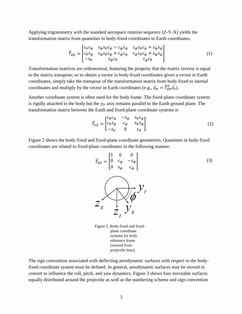
Another coordinate system is often used for the body frame. The fixed-plane coordinate system
is rigidly attached to the body but the axis remains parallel to the Earth ground plane. The
transformation matrix between the Earth and fixed-plane coordinate systems is
(2)
Figure 2 shows the body-fixed and fixed-plane coordinate geometries. Quantities in body-fixed
coordinates are related to fixed-plane coordinates in the following manner.
(3)
Figure 2. Body-fixed and fixed-
plane coordinate
systems for body
reference frame
(viewed from
projectile base).
The sign convention associated with deflecting aerodynamic surfaces with respect to the body-
fixed coordinate system must be defined. In general, aerodynamic surfaces may be moved in
concert to influence the roll, pitch, and yaw dynamics. Figure 3 shows four moveable surfaces
equally distributed around the projectile as well as the numbering scheme and sign convention

4
associated with the trailing edge. The moveable aerodynamic surfaces are numbered starting
with the surface with smallest roll angle and proceeding with increasing roll angle. Deflection of
all moveable aerodynamic surfaces with a positive sense produces negative roll acceleration.
Figure 3. Moveable aerodynamic surface numbering scheme
and trailing edge deflection sign convention
(viewed from projectile base).
Individual moveable aerodynamic surfaces combine to yield effective roll, pitch, and yaw
deflections. The drag deflections are not used in the maneuver scheme.
(4)
Rearranging equation 4 provides individual moveable aerodynamic surface deflections in terms
of roll, pitch, and yaw deflections.
5
(5)
2.2 Nonlinear Flight Dynamic Modeling
Rigid body projectile flight states are center-of-gravity position , attitude
, body translational velocity , and body rotational velocity .
Kinematics provides the relationships between motion in the body and inertial frames.
Translational and rotational kinematics for the body-fixed coordinate system (Murphy, 1963;
McCoy, 1999; Nicolaides, 1963) are
(6)
(7)
Newton’s second law of motion may be applied to derive the dynamics of a rigid-body projectile
in flight. The translational dynamics may be expressed in body-fixed coordinates (Murphy, 1963;
McCoy, 1999; Nicolaides, 1963):
(8)
(9)
The forces are comprised of aerodynamic and gravity (
) terms. Moments
are solely aerodynamic.
Expressing the kinematics and dynamics in fixed-plane coordinates often offers advantages in
terms of numerical run time. The highest resolved frequency in the fixed-plane formulation is the
pitch/yaw rate, so some mass asymmetries, high spin-rate applications, or control mechanisms
6
that change at a spin rate that is higher than the pitch/yaw rate may not be modeled properly. In
the fixed-plane equations of motion that follow, quantities with a tilde are in fixed-plane
coordinates.
(10)
(11)
(12)
(13)
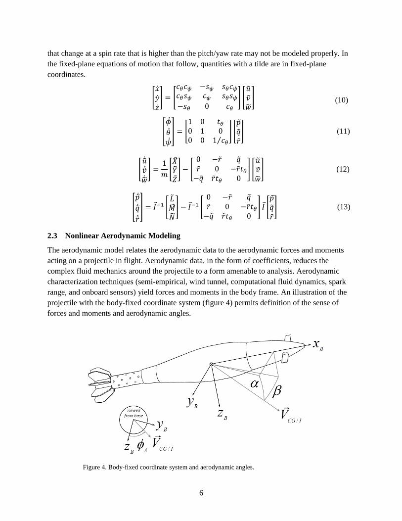
2.3 Nonlinear Aerodynamic Modeling
The aerodynamic model relates the aerodynamic data to the aerodynamic forces and moments
acting on a projectile in flight. Aerodynamic data, in the form of coefficients, reduces the
complex fluid mechanics around the projectile to a form amenable to analysis. Aerodynamic
characterization techniques (semi-empirical, wind tunnel, computational fluid dynamics, spark
range, and onboard sensors) yield forces and moments in the body frame. An illustration of the
projectile with the body-fixed coordinate system (figure 4) permits definition of the sense of
forces and moments and aerodynamic angles.
Figure 4. Body-fixed coordinate system and aerodynamic angles.

7
Aerodynamic angles are computed based on the body-fixed velocity components. The pitch
angle of attack (or sometimes just angle of attack) is defined as
(14)
The yaw angle of attack (or, sometimes, sideslip angle) is
(15)
The aerodynamic roll angle is
(16)
Finally, the total angle of attack is the root-square-sum of the pitch and yaw angles of attack:
(17)
Aerodynamic angles may also be computed in fixed-plane coordinates by replacing the body-
fixed coordinate velocities in equations 14–17 for aerodynamic angles with the corresponding
fixed-plane coordinate velocities.
Total aerodynamic forces and moments are separated into rigid and moveable aerodynamic
surfaces.
Rigid aerodynamic surface forces include static (linear and nonlinear) and dynamic terms.
Symbols in parenthesis indicate functional form of aerodynamic coefficients. The dynamic
pressure is
and the aerodynamic reference area is
, where is the projectile
diameter and is the total velocity.
(18)
(19)
(20)
Rigid aerodynamic surface moments include static (linear and nonlinear) and dynamic terms.
The pitching moment accounts for a center of gravity ( ) that has been shifted from the center
of gravity ( ) used to obtain the aerodynamic data. The center of gravity is measured from
the nose and is given in units of calibers.

8
(21)
(22)
(23)
The following approach may be used to calculate moveable aerodynamic surface forces and
moments for the blade. First, compute local velocity at each blade from center-of-pressure
data (CP, measured in calibers forward of CG), blade geometry ( ), and rigid-body states
using the equation relating the velocity of two fixed points on a rigid body.
(24)
where , , and
. The axial and
radial center of pressure of the moveable aerodynamic surface is a function of Mach number and
lifting surface deflection angle .
Obtain local velocity at each blade in the blade coordinate system using the transformation
matrix:
(25)
(26)
Calculate local blade angle of attack from the local velocity in each blade coordinate system:
(27)

9
Determine lifting surface aerodynamic coefficients:
(28)
(29)
(30)
(31)
Compute blade axial and normal force and roll and pitching moment:
(32)
(33)
(34)
(35)
Transform these blade forces and moments in the blade coordinate system to the body-fixed
coordinate system:
(36)
(37)
This aerodynamic model only serves as a framework since the amount, source, and type of
aerodynamic data, as well as flight phenomena such as interactions, dependence on aerodynamic
roll angle, etc., are specific to a particular airframe at a given stage in development.
2.4 Nonlinear Actuator Dynamic Modeling
Actuator dynamics are modeled as a first-order system with time delay and bias.
(38)

10
This modeling approach is consistent with experimental characterizations of low-cost actuation
technology, as seen in figure 5. The appropriate actuator model must be adjusted for a specific
problem through experiments and system identification. Actuator dynamics may also be
examined and coupled with projectile flight dynamics at a more fundamental level (Fresconi
et al., 2011).
Figure 5. Experimental actuator characterization.
2.5 Nonlinear Measurement Modeling
Measurements provide feedback necessary for projectile guidance. Accelerometers, angular rate
sensors, magnetometers, and imagers are the primary measurements of interest. A schematic of
an arbitrary sensor at point M with axes oriented relative to the body-fixed coordinate system is
shown in figure 6.

11
Figure 6. Body-fixed and measurement coordinate systems.
The specific aerodynamic force in the body frame, the quantity measured by an accelerometer,
can be expressed in terms of Earth or body-fixed states by applying Newton’s second law.
(39)
The equation for the acceleration of two fixed points on a rigid body may be used to model the
accelerometer off the projectile CG (using body-fixed states).
(40)
Integrated sensors suffer from errors in scale factor, misalignment, misposition, bias, and noise.
An expression for an accelerometer corrupted by these errors can be developed.
(41)
Angular rate sensors measure the angular velocity of the body with respect to the inertial frame
in body-fixed coordinates. A model for angular rate sensors with scale factor, misalignment,
bias, and noise errors is
(42)
12
Magnetometers observe the local Earth’s magnetic field. Ignoring induced electromagnetic
effects (spinning ferrous body, actuators, etc.), a model for the magnetometer includes scale
factor, misalignment, bias, and noise errors.
(43)
The scale factor matrix for any sensor can be written as the identity matrix with a scale factor
error unique to each orthogonal axis.
(44)
The transformation from any sensor axes to the body coordinate system, including misalignment
errors, is as follows.
(45)
The bias error of some sensors may feature a term due to the power-up process and an additional
term that drifts in flight and can be modeled with a Markov process.
(46)
The equation for the update of a Markov process is
(47)
with the correlation
, where is the sample time and is the time constant.
An imager model can be constructed by first defining the geometry in figure 7 between the Earth
and line-of-sight (LOS) coordinate systems associated with the inertial frame and the body-fixed
coordinate system associated with the body frame.

13
Figure 7. Earth, LOS, and body-fixed coordinate systems.
The relative position of the target and projectile in the inertial frame is
(48)
The angles of the LOS coordinate system with respect to the Earth coordinate system are
(49)
(50)
The transformation matrix from Earth to LOS coordinates may be formed based on the angles
between the coordinate systems.
(51)
The velocity of the target with respect to the projectile in the inertial frame is
(52)
The relative position in body-fixed coordinates can be written given the transformation matrix.

14
(53)
Using the relative position in body-fixed coordinates, the angles of the target centroid as seen by
a strapdown seeker can be determined. Bias and noise may be added for modeling real-world
measurements.
(54)
(55)
Angular velocity of the LOS coordinate system can be derived given the relation (Greenwood,
1965)
(56)
Substituting the expression for the relative position and velocity of the target with respect to the
projectile in the Earth coordinate system in equation 56 for the angular velocity yields the
angular velocity components of the LOS coordinate system.
(57)
(58)
Transforming the LOS rates to the LOS coordinate system and incorporating bias and noise
errors characteristic of a practical imager yields
(59)
(60)
2.6 Linear Flight Dynamic Modeling
The nonlinear equations of motion for projectile flight are linearized by making a few
assumptions (Murphy, 1963; Etkin, 1972). Off-diagonal inertia tensor terms are small compared
with the diagonal terms. Products of dynamic states (i.e., ) are neglected. Total
angle of attack is small, and aerodynamic normal force and pitching moment trims, as well as
side forces and side moments, are neglected so that only linear terms remain in the aerodynamic
model.

15
Additionally, the aerodynamic contribution of the moveable aerodynamic surfaces is cast in
terms of the deflections for roll, pitch, and yaw.
The linear roll dynamics are expressed in equation 61. The static roll moment remains because of
the ability of fin cant to maintain ballistic accuracy over unguided portions of the flight.
(61)
The linear pitch rate dynamics:
(62)
Finally, the linear pitch acceleration:
(63)
The linear yaw rate and yaw acceleration have a form similar to the linear pitch rate and pitch
acceleration dynamics, respectively, and are provided later.
Taking the time derivative of the linear pitch acceleration dynamics with the linearization
assumptions (body frame is stationary when neglecting products of dynamic states) yields
(64)
Figure 8 shows the relationship between the Euler angle, angle of attack, and velocity vector
angle in the pitch plane.
Figure 8. Relationship between Euler angle, angle of attack, and velocity vector angle in pitch plane.

16
From figure 8 we see that
(65)
Taking the time derivative of the expression above and assuming that the body frame is
stationary, the rate of change of the Euler angle is the body pitch rate.
(66)
We know from general curvilinear motion that the acceleration component normal to the velocity
vector can be obtained by the product of the radius of curvature and square of the angular rate.
Additionally, this expression can be manipulated by the definition of the velocity and the
equation for the rate of change of the velocity vector.
(67)
Solving equation 67 for the rate of change of the angle of attack results in
(68)
Substituting equations 68 into 64 provides an expression for pitch acceleration rate. This
equation has pitch acceleration (measurable with an accelerometer) rather than angle of attack
(not easily measurable) as a dependent variable.
(69)
Next, the pitch rate dynamics and the pitch acceleration dynamics are premultiplied with an
appropriate factor and subtracted.
(70)
Solving equation 70 for the pitch rate provides an expression with pitch acceleration (measurable
with an accelerometer) rather than angle of attack (not easily measurable) as a dependent
variable.
(71)
A similar exercise yields the yaw rate and yaw acceleration rate dynamics. Some sign changes
from the pitch dynamics occur on a few terms in the yaw dynamics.
(72)

17
(73)
The linear flight dynamics are now cast into state space form for state dynamics
(74)
and the measurements.
(75)
The state vector is defined:
(76)
The controls are the roll, pitch, and yaw deflections.
(77)
The state transition matrix follows. The roll angle dynamics are incorporated by simple
integration of the roll rate.
(78)
The controls matrix:
(79)
The static roll moment appears as a steady-state term that is independent of the state and control
vector.
(80)
The measurement matrix is simply the identity matrix ( ) since feedback consists of
accelerometers, angular rate sensors, and magnetometers. All states are directly measureable

18
except for roll angle, which would come from integrating an angular rate sensor or using only a
magnetometer or some combination of magnetometer, accelerometer, and angular rate sensor in
an observer. For this formulation, .
2.7 Linear Actuator Modeling
The nonlinear actuator model is composed of a first-order system, time delay, and bias. The
ordinary differential equation of the first-order model for the actuator is
(81)
The transfer function form of a first-order system is used to represent the first-order actuator
dynamics.
(82)
The Laplace transform of a time delay is
(83)
We seek to approximate this exponential in frequency space to build a linear model for the
actuator time delay. The Maclaurin series approximation to a function is
(84)
Applying the Maclaurin series to the Laplace transform of the time delay results in
(85)
Pade approximants consist of polynomial expansions in the numerator and denominator.
(86)
The coefficients in the numerator and denominator can be found through recursive relationships
by setting the Pade expansions equal to the Maclaurin series and solving for the coefficients for
polynomials of like order.
(87)
The transfer function form of the Pade approximant is
(88)

19
A plot of a 12th-order Pade approximation and the exact time delay of 1 s for a step response are
shown in figure 9. Comparing these two curves illustrates the error associated with
approximating the nonlinearity with high-order polynomials.
Figure 9. Approximate and exact response with time delay.
Applying superposition to the linear models for the time delay and first-order system expressed
in transfer function form is shown in block diagram form in figure 10. This enables modeling the
actual deflection given the commanded deflection.
Figure 10. Block diagram of time delay and first-order system dynamics.
Multiplying transfer functions yields equation 89. Assume that .

20
(89)
The transfer function for the time delay and first-order system can be expressed in a chain rule
form to eventually yield a state-space model in control canonical form.
(90)
The right-most term is
(91)
Converting from frequency space to time space produces a high-order ordinary differential
equation.
(92)
The left-most term in equation 91 is
(93)
The time response of the actuator with time delay and first-order dynamics is obtained by
(94)
A state-space model of the actuator with time delay and first-order dynamics was constructed
with the following state vector.
(95)
The control for the actuator is simply the deflection command.
(96)
Arranging terms in the differential equations provided in equation 92 with the definitions of the
state and control vectors produces the state transition matrix.

21
(97)
Likewise, the control matrix can be formed.
(98)
The measurement matrix, ( ):
(99)
The exact nonlinear and linear approximation ( for Pade approximant) to the time delay
(1 s) with first-order system (1-s time constant) are presented in figure 11. There is little error
between the approximate and exact solutions for this case.
Figure 11. Approximate and exact response with time delay and first-order system.

22
The state-space model of the actuator with time delay and first-order dynamics is for a given
deflection. The flight model features roll, pitch, and yaw deflections. A comprehensive roll,
pitch, and yaw state-space model may be constructed by building on the individual state-space
model outlined in equations 95–99. The state vector and control vector is composed of three
subvectors.
(100)
(101)
The state transition, control, and measurement matrices are
(102)
(103)
(104)
2.8 Linear System Modeling with Time Delay
Realization of the actuator with time delay and first-order dynamics with the flight dynamics
yields a system model. The block diagram of the combined system is presented in figure 12.
Figure 12. Block diagram of actuator time delay and first-order system
and flight dynamics.
Figure 12 shows that the response of the actuator drives the flight behavior. This mathematical
relationship allows coupling of the actuator and the flight dynamics.
(105)

23
The state and control vectors are made up of the flight and actuator with time delay and first-
order dynamics, as derived earlier.
(106)
(107)
The state transition matrix is composed of the flight and actuator state transition matrix and an
additional term in the top right of the matrix due to the coupling as given in equation 108.
(108)
The coupling reduces the controls matrix to the following equation. The top-left portion of the
matrix is a block of zeros since the coupling has picked off the controls matrix for the flight
model.
(109)
The vector is a concatenation of the vector followed by a row of zeros the length of .
The measurement matrix for the system is
(110)
2.9 Linear System Modeling Without Time Delay
Another useful linear system model is for the flight dynamics and first-order actuator dynamics
without time delay. The state vector for this system is
(111)
The control vector is
(112)
The state transition matrix is formed based on the dynamic modeling performed for the flight
dynamics and first-order actuator.
24
(113)
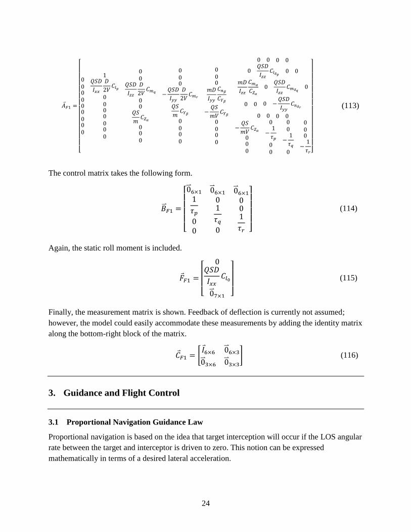
The control matrix takes the following form.
(114)
Again, the static roll moment is included.
(115)
Finally, the measurement matrix is shown. Feedback of deflection is currently not assumed;
however, the model could easily accommodate these measurements by adding the identity matrix
along the bottom-right block of the matrix.
(116)
3. Guidance and Flight Control
3.1 Proportional Navigation Guidance Law
Proportional navigation is based on the idea that target interception will occur if the LOS angular
rate between the target and interceptor is driven to zero. This notion can be expressed
mathematically in terms of a desired lateral acceleration.

25
(117)
The gain is usually between 3 and 5. Equation 117 is one representation of proportional
navigation; there are many different variants in the literature (Zarchan, 2007).
The closing velocity is calculated from the projection of the velocity vector onto the line of sight
( axis). Bias and noise errors can be added to the true closing velocity to model measurement
corruption.
(118)
The proportional navigation law with gravity compensation, in body-fixed components, is
(119)
In practice, only lateral acceleration can be altered with aerodynamic control; range-rate
measurements or heuristics supply the closing velocity, angular rate sensors, or magnetometers
supply attitude, and an imager or spot detector provides the LOS rates.
3.2 Optimal Flight Control
The basic structure of a multiple input-multiple output feedback control system is shown in
figure 13. The nonlinear dynamics of the actuator, flight, and measurements are fed back and
combined with a reference to yield an error. Control commands, formed by multiplying this error
by a gain, influence the system dynamics to achieve the desired response.
Figure 13. Block diagram of nonlinear system dynamics with feedback control.
Linear dynamics are often used for control. The block diagram of the linear system dynamics
with feedback control is illustrated in figure 14. Nonlinear dynamics of the actuator, flight, and
measurements have been replaced by linear system transfer functions. An observer could be
designed and placed in the feedback path; however, this is outside the scope of this report.

26
Figure 14. Block diagram of linear system dynamics with feedback
control.
The relationship between the transfer function and state space model is obtained by manipulating
the Laplace transform of the basic state space model equations.
(120)
The linear system model without time delay that was derived earlier can be used for control
purposes. The state space model can be defined with , , , ,
, , and . The linear system model with time delay derived earlier may
also be used for control purposes. If necessary, integral control could be added to this
formulation by augmenting the state vector with additional states such as , , and with
simple dynamics based in integrating states already in the system dynamics (e.g., ).
The nonlinear measurement models outlined previously can be used to express the six feedback
states.
(121)
For this problem, the desired response is to regulate the roll angle to any of four angles
determined by symmetry (based on flying skid-to-turn in an “X” configuration), maintain zero
roll rate, pitch rate, and yaw rate, and achieve the lateral accelerations dictated by the guidance
law. Mathematically, the reference signal is expressed as
(122)
Controlling roll rate to nonzero values as a means to incorporate low-cost measurement and
actuation technologies is accommodated within the current framework by setting the roll angle
gain to zero.
Manipulation of the roll angle error signal is accomplished by the following function to ensure
that the roll angle is controlled to the closest symmetry location.
(123)
The number of roll angles for configuration symmetry is usually four. Figure 15 illustrates the
manner in which the roll angle is converted into the roll angle error signal.

27
Figure 15. Roll angle and roll angle error.
A variety of control techniques may be applied given the linear actuator and flight dynamics,
measurement models, and feedback control structure presented. A linear quadratic regulator
derived using optimal control theory was chosen. In the linear quadratic regulator development,
the control command is based on minimizing a cost function.
(124)
The weightings for the tracking error and control effort are positive semi-definite and allow
the designer to balance tracking each desired state with specific control demand. The control law
that minimizes the cost function is
(125)
The gain matrix can be found through the control effort weighting, the controls matrix, and the
matrix .
(126)
The matrix is obtained by solving the algebraic matrix Riccatti equation.
(127)

28
3.3 Smith Predictor
Delays between the time of commanded control and when the effect of control is realized in the
system dynamics occur because of a variety of physical processes and can add significant
difficulty to the control problem. Additionally, the time delay magnitude may be higher when
using low-cost technologies, such as commercial-off-the-shelf servomechanisms. The Smith
predictor is a control strategy for dealing with time delays (Smith, 1959). A block diagram of the
Smith predictor algorithm for the projectile problem is given in figure 16. The linear system
model without and with time delay are used in augmenting the feedback system, and the
nonlinear actuator, flight, and measurement models represent ground truth in simulation.
Measurements are a function of the flight states and controls.
Figure 16. Smith predictor.
The basic idea of the Smith predictor is that a model of the system dynamics with time delay can
be used to negate the true system dynamics with time delay. Controllers that do not inherently
consider the time delay (such as the linear quadratic regulator) can then be applied since the
resulting feedback signal has the time delay effectively removed.
The linear system models without and with time delay are propagated forward in time in
implementation of the Smith predictor. Feedback is altered by the following equation.
(128)
The Smith predictor is sensitive to modeling error and uncertainty in the model parameters. A
modified Smith predictor (Tsai and Tung, 2012) has been proposed that has some disturbance
rejection properties to handle modeling error and uncertain model parameters. The block
diagram of the modified Smith predictor is shown in figure 17.

29
Figure 17. Modified Smith predictor.
Realization can be applied with the block diagram and dynamics (nonlinear and linear) derived
earlier to determine the modified Smith predictor equations. The input to the actuator dynamics
can be found by inspecting the block diagram.
(129)
4. System Characteristics
The theory for the actuator, flight, and measurements and strategy for guidance and flight control
relies heavily on system characteristics. Proper characterization of actuator, flight, and
measurement parameters are essential to efficient guidance of highly maneuverable airframes to
moving targets. An illustration of a high-maneuverability airframe is presented at the top of
figure 18. This fin-stabilized, canard-controlled projectile has a diameter of 83 mm and is
5 cal. long. Drag is minimized through a 7° boattail, and the hemispherical nose necessary for
packaging guidance, navigation, and control components is satisfactory since only subsonic
flight is intended. Flying a skid-to-turn configuration enables interception of more maneuverable
targets since the projectile does not have to roll into the desired plane prior to pulling lateral
maneuvers as in a bank-to-turn scenario. While canards complicate the aerodynamic
characterization due to flow interactions, the projectile features more maneuverability than
fin-only control. Fin cant improves accuracy over unguided portions of flight.
Adding more aerodynamic surface area through the use of deploying wings is a way to further
enhance maneuverability. The bottom of figure 18 sketches some concepts for canard control of
body-fin-wing configurations. There are practical challenges associated with reliable deployment
and integration with other subsystems such as warheads.

30
Figure 18. High-maneuverability airframe.
The mass properties (mean and uncertainty) of this projectile are given in table 1.
Table 1. Mass properties.
Property Unit Unit
0.083 m 0.12 %
0.219 m from nose 0.12 %
0.427 m 0.12 %
7.31 kg 0.41 %
0.0106 kg-m2
0.88 %
0.0690 kg-m2
0.71 %

31
The launch and flight are subsonic. Some aerodynamic data for this airframe, as obtained from
computational fluid dynamics simulations at Mach 0.65, are provided in table 2.
Table 2. Aerodynamic data at Mach 0.65 for CGN,A = 0.219 m from nose.
Property Unit Unit
0.320 — 0.86 %
10.842 1/rad 1 %
–4.177 1/rad 2 %
0.0667 — 5 %
–10.392 — 5 %
–150 — 15 %
0.893
Calibers
forward
CG
2 %
0.848
Calibers
from spin
axis
2 %
0.0042 — 0.86 %
–0.808 1/rad 5 %
0.953 1/rad 1 %
0.851 1/rad 2 %
A variety of actuation technologies (electric, pneumatic, piezoelectric, etc.) may be applied to
deflect canards. Specific actuator characteristics may be defined through a cost-performance
trade study. For the purposes of this report, actuator parameters given in table 3 are
representative of low-cost, high-volume servomechanisms. The update rate of the actuator was
500 Hz.
Table 3. Actuator properties.
Property Unit Unit
0.015 sec 20 %
0.030 sec 20 %
— — 1 °
Accelerometers, angular rate sensors, magnetometers, and imagers provide measurements for
this problem. Similar to the actuation technology, cost-performance trades can be used to
identify specific devices; however, some nominal measurement characteristics are given in
table 4. Feedback update rate was 1000 Hz.

32
Table 4. Measurement properties.
Property Unit
(integrated
misalignment) 0.5 degree
(accelerometer) 0.0005 m
(accelerometer) 1.0 %
(accelerometer) 1.0 m/s2
(gyroscope) 2.1 %
(gyroscope) 0.1 rad/s
(imager boresight
angles) 10 degree
(imager boresight
angular rates) 0.01 rad/s
(closing velocity) 0.1 m/s
The variation in the initial conditions of the projectile and target are provided in table 5. The
target was modeled as a constant velocity, straight-line motion.
Table 5. Launch variation.
Property Unit
(uniform) rad
0.004014 rad
0.005411 rad
3.7 m/s
1.0 rad/s
1.0 rad/s
1.0 rad/s
Target position 2.0 m
Target velocity 0.5 m/s
The controller parameters, found via stability analysis and tuning in the linear and nonlinear
simulations, are given in table 6. The update rate of the flight controller was 500 Hz.
Table 6. Controller properties.
Property Value
10
0.05
100
0.05
10
10
0.8
0.8

33
5. Results and Discussion
The theory for the flight, actuator, and measurements were implemented in simulation. A fourth-
order Runge-Kutta integrator was applied. The 1962 International Standard Atmosphere was
used to determine air density and sound speed. Wind speed variations were taken according to
ballistic range measurements such as artillery meteorological data staleness. A Dryden wind
turbulence model incorporated fluctuations of wind throughout flight.
A stability analysis was undertaken. The eigenvalues in figure 19 were shaped for desired
performance with the linear flight and first-order actuator model and system characteristics
provided earlier. Inspection of the controlled and uncontrolled (ballistic) data illustrates how the
control increases the damping and frequency of the response. This airframe is statically unstable;
therefore, the uncontrolled response has positive real roots.
Figure 19. Characteristic values of linear system dynamics.
Linear simulations were performed to assess ballistic flight behavior and tune the flight
controller for the desired performance. The flight control algorithm was implemented in
simulation. The results in figures 19–21 show performance of the linear quadratic regulator for a
time delay of zero with nominal initial conditions.

34
The roll dynamics and control demand are provided in figure 20. Inspection of the roll angle data
illustrates the achieved roll angle, the roll error signal, and the desired roll signal. The roll angle
error signal has been manipulated as outlined previously to maintain configuration symmetry of
the moveable aerodynamic surfaces (i.e., the error is not the difference between the achieved and
desired signals as shown in the plot). The roll rate plot provides similar data (desired, achieved,
error). The commanded and achieved (based on actuator dynamics) roll deflection angles are also
given. Overall, this control design yields satisfactory roll response with reasonable control effort.
Adequate control of the roll dynamics is necessary for proper pitch and yaw control.
Figure 20. Linear roll system dynamics response and deflection commands (linear quadratic regulator control
with tD = 0).
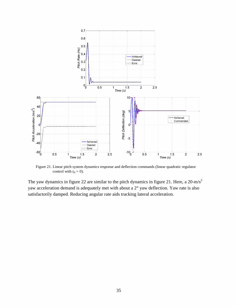
Figure 21 shows the pitch dynamics for a desired pitch acceleration of 50 m/s2. Pitch deflections
oscillate initially to sufficiently damp angular rate. The desired pitch acceleration is tracked to
less than 1 m/s2
error by deflecting in pitch to about 5°.
35
Figure 21. Linear pitch system dynamics response and deflection commands (linear quadratic regulator
control with tD = 0).
The yaw dynamics in figure 22 are similar to the pitch dynamics in figure 21. Here, a 20-m/s2
yaw acceleration demand is adequately met with about a 2° yaw deflection. Yaw rate is also
satisfactorily damped. Reducing angular rate aids tracking lateral acceleration.

36
Figure 22. Linear yaw system dynamics response and deflection commands (linear quadratic regulator
control with tD = 0).
A Monte Carlo study was performed to assess the influence of system uncertainties on the
controlled flight performance with . The initial conditions, mass properties, aerodynamic
coefficients, actuator characteristics, and measurement errors were varied according to the
parameter distributions supplied earlier. Linear simulations were run for each Monte Carlo trial
for 1.5 s, and the errors between the desired and achieved state were tabulated. The mean (shown
in solid circle) and +/- standard deviation (shown in “X”) of these errors is given in figure 23.
Different colors in the figure represent different states. The error budget for the system
uncertainties was scaled by different factors (0.1, 1, 2, 3) for trend analysis. With the exception
of roll angle, the mean controlled state errors do not vary much. Roll angle is biased about 1°–2°
due to the fin cant. This effect could easily be accounted for with some feed-forward action. The
standard deviation of the errors for all states but roll, pitch, and yaw rates grows linearly with the
error budget factor. The angular rate errors are low because the control is effective and damping
moments are active.

37
Figure 23. Linear system simulation – Monte Carlo response trades.
The pitch dynamics are isolated to investigate the effects of time delay. Linear simulations were
performed with a nonzero time delay. The unstable behavior of the linear quadratic regulator for
nonzero time delay is evident in figure 24. Commanded pitch deflections oscillate back and forth
at the saturation levels and produce poor tracking in pitch acceleration and pitch rate.
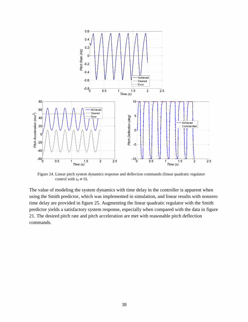
38
Figure 24. Linear pitch system dynamics response and deflection commands (linear quadratic regulator
control with tD 0).
The value of modeling the system dynamics with time delay in the controller is apparent when
using the Smith predictor, which was implemented in simulation, and linear results with nonzero
time delay are provided in figure 25. Augmenting the linear quadratic regulator with the Smith
predictor yields a satisfactory system response, especially when compared with the data in figure
21. The desired pitch rate and pitch acceleration are met with reasonable pitch deflection
commands.

39
Figure 25. Linear pitch system dynamics response and deflection commands (linear quadratic regulator and
Smith control with tD 0).
Nonlinear system simulations were conducted to further investigate the flight control and
demonstrate guidance performance against moving targets. The projectile was launched at sea
level and a muzzle velocity of 250 m/s with the target initially located along the line of fire
1000 m downrange. The target was moving 5 m/s in the cross-range direction.
A sample Monte Carlo trajectory with system characteristics outlined previously is provided in
figure 26. The projectile maneuvers toward the target with a small point of closest approach. The
target moves about 20 m in cross range over approximately 5 s of projectile time of flight.

40
Figure 26. Nonlinear system simulation – trajectory.
The Mach number and pitch and yaw angles of attack are shown in figure 27. The projectile does
not decrease much in Mach over the 5-s flight. The angles of attack, dictated primarily by the
desired lateral accelerations from the guidance law, are low and well within the bounds of the
high-maneuverability airframe.
Figure 27. Nonlinear system simulation – Mach number and angular motion histories.
41
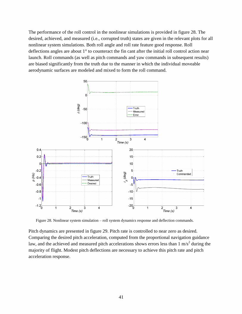
The performance of the roll control in the nonlinear simulations is provided in figure 28. The
desired, achieved, and measured (i.e., corrupted truth) states are given in the relevant plots for all
nonlinear system simulations. Both roll angle and roll rate feature good response. Roll
deflections angles are about 1° to counteract the fin cant after the initial roll control action near
launch. Roll commands (as well as pitch commands and yaw commands in subsequent results)
are biased significantly from the truth due to the manner in which the individual moveable
aerodynamic surfaces are modeled and mixed to form the roll command.
Figure 28. Nonlinear system simulation – roll system dynamics response and deflection commands.
Pitch dynamics are presented in figure 29. Pitch rate is controlled to near zero as desired.
Comparing the desired pitch acceleration, computed from the proportional navigation guidance
law, and the achieved and measured pitch accelerations shows errors less than 1 m/s2 during the
majority of flight. Modest pitch deflections are necessary to achieve this pitch rate and pitch
acceleration response.

42
Figure 29. Nonlinear system simulation – pitch system dynamics response and deflection commands.
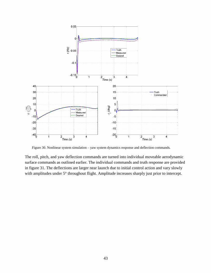
The yaw dynamics shown in figure 30 are similar to the pitch dynamics. Again, desired yaw
angular rate and yaw acceleration are satisfactorily achieved with small yaw deflection
commands.
43
Figure 30. Nonlinear system simulation – yaw system dynamics response and deflection commands.
The roll, pitch, and yaw deflection commands are turned into individual moveable aerodynamic
surface commands as outlined earlier. The individual commands and truth response are provided
in figure 31. The deflections are larger near launch due to initial control action and vary slowly
with amplitudes under 5° throughout flight. Amplitude increases sharply just prior to intercept.

44
Figure 31. Nonlinear system simulation – individual canard deflection commands.
The motion of the target as measured by an imager is shown in figure 32 (open circle denotes
initial measurement and “X” denotes final measurement). The controlled flight dynamics
produce a complex pattern in the image plane. The angles are relatively small (less than 10°) and
the imager angular error does not converge to zero for successful target intercept.

45
Figure 32. Nonlinear system simulation – target centroid measured by imager.
A batch of 100 Monte Carlo flights were simulated, and the point of closest approach was
tabulated. Overall, 94% of the projectiles flew within 0.1 m of the moving target. A histogram of
the flights within 0.1 m of the target is provided in figure 33. Implementing the theoretical
models outlined previously in simulation with the current characteristics for this GNC system
yields miss distances often less than 0.02 m.

46
Figure 33. Nonlinear system simulation – Monte Carlo miss distance.
Monte Carlo trials were performed in the nonlinear system simulation to quantify the
relationship between guided performance and system uncertainties. Again, the parameter
distributions outlined previously were used in the simulations. All uncertainties were scaled by a
factor to illustrate trends. Monte Carlo simulations were conducted by isolating each parameter
category (e.g., initial conditions, mass properties) and running all parameter errors together.
These results are provided in figure 34. All average miss distances are less than 0.02 m.
Comparing the initial-condition-only cases with the all-parameter-error cases suggests little
contribution from initial condition variations. Miss distance will be influenced by initial
conditions if the combination of targeting and fire control are so poor that the projectile cannot
physically intercept the target.
Mass properties and aerodynamics uncertainties do not greatly contribute to the overall miss
distance. Indeed, Monte Carlo cases were able to be run with 5 and 10 times the nominal error
budget for these categories without appreciable changes in the miss distance. Intolerance of the
miss distance to these parameters is due to the nature of the feedback control strategy and the
magnitude of round-to-round physical (mass and aerodynamics) variability.

47
Figure 34. Nonlinear system simulation – Monte Carlo miss distance trades.
Miss distance is also not driven by the actuator characteristics and variability for this system.
Miss distances for the actuator-only cases are relatively small compared with the all-parameter
cases. Additionally, miss distance does not vary significantly even when the nominal variability
is scaled by a factor of 3.
Measurement errors are the main contributor to miss distance. Monte Carlo miss distances for
the measurement-only errors are similar in magnitude to the all-parameter cases. These results
suggest proper measurement design (e.g., sensors, electronics) is critical to guided system
performance.

48
6. Conclusions and Recommendations
This report detailed theory concerning guided flight that is essential to constructing simulations
for researching low-cost, high-maneuverability projectiles. The nonlinear equations of motion for
projectile flight in body-fixed and fixed-plane coordinates were presented. Aerodynamic
modeling included definitions of the angles of attack, linear and nonlinear static and dynamic
terms, and a force and moment model for general moveable aerodynamic surfaces. Actuator
dynamic modeling was performed. Nonlinear measurement models were discussed. Flight model
states were manipulated to simulate the response of accelerometers, gyroscopes, magnetometers,
and imagers. These feedback measurements are necessary for guidance and flight control.
System identification for actuators and measurements is critical to adjusting models as
appropriate for advanced precision concepts.
Manipulation of these nonlinear models into linear system models were undertaken for airframe
characterization and control design.
A framework for guidance and flight control was built. The family of proportional navigation
guidance laws was introduced. The basic feedback control system for guided projectiles was
described. This report developed a suite of high-fidelity model-based flight controllers.
System characteristics were provided for reproduction of results. Aerodynamic, actuator, and
measurement parameter estimation are crucial to successful precision munitions concept
maturation.
The theory and guidance and flight control strategy was implemented in simulation to illustrate
essential elements of low-cost, high-maneuverability GNC systems. Linear analysis allowed
tuning controllers. The guidance and flight control performance were more comprehensively
evaluated in the nonlinear simulations. Results indicated satisfactory system response with
reasonable control input. When time delays are significant, it is necessary to explicitly model
these effects in the control.
Future efforts focus on applying and adapting this guidance and flight control approach to
practical low-cost, high-maneuverability U.S. Army projectiles. Advanced guidance and flight
control techniques are also being investigated to further reduce the cost of the actuation and
measurement technology and increase maneuverability.
49
7. References
Davis, B.; Malejko, G.; Dorhn, R.; Owens, S.; Harkins, T.; Bischer, G. Addressing the
Challenges of a Thruster-Based Precision Guided Mortar Munition With the Use of
Embedded Telemetry Instrumentation. ITEA Journal 2009, 30, 117–125.
Etkin, B. Dynamics of Atmospheric Flight; John Wiley & Sons: Hoboken, NJ, 1972.
Fresconi, F. E. Guidance and Control of a Projectile with Reduced Sensor and Actuator
Requirements. Journal of Guidance, Control, and Dynamics 2011, 34 (6), 1757–1766.
Fresconi, F. E.; Cooper, G. R.; Celmins, I.; DeSpirito, J.; Costello, M. Flight Mechanics of a
Novel Guided Spin-Stabilized Projectile Concept. Journal of Aerospace Engineering 2011,
226, 327–340.
Greenwood, D. T. Principles of Dynamics; Prentice-Hall, Inc.: Englewood Cliffs, NJ, 1965.
Grubb, N. D.; Belcher, M. W. Excalibur: New Precision Engagement Asset in the Warfighter.
Fires 2008, October–December, 14–15.
McCoy, R. L. Modern Exterior Ballistics; Schiffer Publishing Ltd.: Atlen, PA, 1999.
Moorhead, J. S. Precision Guidance Kits (PGKs): Improving the Accuracy of Conventional
Cannon Rounds. Field Artillery 2007, January–February, 31–33.
Morrison, P. H.; Amberntson, D. S. Guidance and Control of a Cannon-Launched Guided
Projectile. Journal of Spacecraft and Rockets 1977, 14 (6), 328–334.
Murphy, C. H. Free Flight Motion of Symmetric Missiles; BRL-TR-1216; U.S. Army Ballistics
Research Laboratory: Aberdeen Proving Ground, MD, 1963.
Nicolaides, J. On Missile Flight Dynamics. Ph.D Dissertation, Catholic University of America,
Washington, DC, 1963.
Smith, O. J. M. A Controller to Overcome Dead Time. ISA Journal 1959, 6, 28–33.
Tsai, M.; Tung, P. A Robust Disturbance Reduction Scheme for Linear Small Delay Systems
With Disturbances of Unknown Frequencies. ISA Transactions 2012, 51, 362–372.
Zarchan, P. Tactical and Strategic Missile Guidance, 5th ed.; American Institute of Aeronautics
and Astronautics: Reston, VA, 2007.

NO. OF NO. OF
COPIES ORGANIZATION COPIES ORGANIZATION
50
1 DEFENSE TECHNICAL
(PDF) INFORMATION CTR
DTIC OCA
1 DIRECTOR
(PDF) US ARMY RESEARCH LAB
IMAL HRA
1 DIRECTOR
(PDF) US ARMY RESEARCH LAB
RDRL CIO LL
1 GOVT PRINTG OFC
(PDF) A MALHOTRA
2 ARO
(PDF) S STANTON
B GLAZ
6 RDECOM AMRDEC
(PDF) L AUMAN
J DOYLE
S DUNBAR
B GRANTHAM
M MCDANIEL
C ROSEMA
1 RDECOM ECBC
(PDF) D WEBER
40 RDECOM ARDEC
(PDF) M BAKER
G BISCHER
D CARLUCCI
J CHEUNG
S K CHUNG
D L CLER
B DEFRANCO
D DEMELLA
M DUCA
P FERLAZZO
G FLEMING
R FULLERTON
R GORMAN
R GRANITZKI
N GRAY
J C GRAU
M HOHIL
M HOLLIS
R HOOKE
W KOENIG
A LICHTENBERG-SCANLAN
S LONGO
E LOGSDON
M LUCIANO
P MAGNOTTI
G MALEJKO
M MARSH
G MINER
J MURNANE
M PALATHINGAL
D PANHORST
A PIZZA
T RECCHIA
G SCHLENK
B SMITH
C STOUT
W TOLEDO
E VAZQUEZ
L VO
C WILSON
2 PEO AMMO
(PDF) C GRASSANO
P MANZ
3 PM CAS
(PDF) R KIEBLER
P BURKE
M BURKE
1 MCOE
(PDF) A WRIGHT
2 ONR
(PDF) P CONOLLY
D SIMONS
2 NSWCDD
(PDF) L STEELMAN
K PAMADI
1 AFOSR EOARD
(PDF) G ABATE
1 MARCORSYSCOM
(PDF) P FREEMYERS
2 DARPA
(PDF) J DUNN
K MASSEY

NO. OF NO. OF
COPIES ORGANIZATION COPIES ORGANIZATION
51
2 DRAPER LAB
(PDF) C GIBSON
G THOREN
1 GTRI
(PDF) A LOVAS
3 ISL
(PDF) C BERNER
S THEODOULIS
P WERNERT
1 DRDC
(PDF) D CORRIVEAU
2 GEORGIA INST OF TECHLGY
(PDF) M COSTELLO
J ROGERS
1 ROSE HULMAN INST OF TECHLGY
(PDF) B BURCHETT
1 AEROPREDICTION INC
(PDF) F MOORE
1 ARROW TECH
(PDF) W HATHAWAY
3 ATK
(PDF) R DOHRN
B BECKER
S OWENS
3 BAE
(PDF) B GOODELL
P JANKE
O QUORTRUP
1 GD OTS
(PDF) D EDMONDS
3 UTAS
(PDF) P FRANZ
S ROUEN
M WILSON
ABERDEEN PROVING GROUND
55 DIR USARL
(PDF) RDRL WM
P J BAKER
RDRL WML
P J PEREGINO M J ZOLTOSKI
RDRL WML A
M ARTHUR
W F OBERLE III
R PEARSON
L STROHM
RDRL WML B
N J TRIVEDI
RDRL WML C
S A AUBERT
RDRL WML D
R A BEYER
A BRANT
J COLBURN
M NUSCA
Z WINGARD
RDRL WML E
V A BHAGWANDIN
I CELMINS
J DESPIRITO
L D FAIRFAX
F E FRESCONI III
J M GARNER
B J GUIDOS JR
K R HEAVEY
R M KEPPINGER
G S OBERLIN
T PUCKETT
J SAHU
S I SILTON
P WEINACHT
RDRL WML F
B ALLIK
G BROWN
E BUKOWSKI
B S DAVIS
M DON
M HAMAOUI
K HUBBARD
M ILG
B KLINE J MALEY
C MILLER
P MULLER
B NELSON
B TOPPER
RDRL WML G
A ABRAHAMIAN
M BERMAN
M CHEN
W DRYSDALE
M MINNICINO
J T SOUTH

NO. OF
COPIES ORGANIZATION
52
RDRL WML H
T EHLERS
M FERMEN-COKER
J F NEWILL
R PHILABAUM
R SUMMERS
RDRL WMM
J S ZABINSKI
RDRL WMP
D H LYON
2 DSTL
(PDF) T BIRCH
R CHAPLIN