THERMAL RESIDUAL STRESSES IN

HOT-ROLLED STEEL MEMBERS

by

Goran A. Alpsten

Fritz Engineering LaboratoryDepartment of Civil Engineering

Lehigh UniversityBethlehem, Pennsylvania

December, 1968

Fritz Laboratory Report No. 337.3

337.3 TABLE OF CONTENTS

THERMAL STRESS ANALYSIS 27

Theory and Assumptions 27

Formula~ion of Stress-Strain Equations 28

Mechanical Coefficients 31

Results of Thermal Stress Computations on Plates 33

Results of Thermal Stress Computations on H-Shapes 36

Comparison with Experimental Results 43

ABSTRACT

INTRODUCTION

Purpose and Scope

Short Review of the Manufacturing Procedure

Previous Work

METHOD FOR CALCULATION OF THERMAL RESIDUAL STRESS

TEMPERATURE ANALYSIS

Theory and Assumptions

Formulation of Finite-Difference Relationships

Thermo-Physical Coefficients

Results of Temperature Computations

Results of Temperature Measurements

SUMMARY AND CONCLUSIONS

ACKNOWLEDGMENTS

NOMENCLATURE

FIGURES

REFERENCES

1

3

3

5

7

11

14

14

16

18

20

24

46

51

53

55

112

337.3

ABSTRACT

A method for calculating thermal residual stresses in hot-

rolled steel members is presented. The method is based on a

computation of the temperature and thermal stress distributions

throughout the cooling process using a finite-difference method

and· simulating the actual conditions, including variable material

coefficients.

Several computations of residual stresses in rolled plates

and H-shapes were carried out using an electronic computer with

the purpose of studying (1) the mechanism of formation of thermal

residual stresses, (2) the possible influence of various manu­

facturing conditions upon residual stresses, (3) the effect of

variations in material properties, and (4) the effect of shape

geometry. The eventual aim of this study was to make possible

predictions of thermal residual stresses in hot-rolled plates

and shapes.

From the study it was found that shape geometry and cooling

conditions are the principal factors which influence the forma­

tion of thermal residual stresses in hot-rolled members.

with the predictions.

The computations were correlated with experimental measure­

ments of the temperature distribution during cooling of \H-shapes.

Comparisons were made also with measured residual stress distri-

butions. In general, the experimental results are in conformity

337.3 -2

Since the results obtained theoretically have correlated

well with the experimental data, the method is expected to be of

practical use in the predi~tion of thermal residual stresses in

hot-rolled plates and shapes .. Also, analogous methods should be

useful for the prediction of temperature-time history and resi­

dual stress resulting from other thermal manufacturing and fa~­

rication processes, such as flame-cutting, welding, and heat­

treatment.

INTRODUCTION

residual stresses as well as the factors which influence the for-

Purpose and Scope

Therefore, the actual magnitude and distribution of

Residual stresses in structural members can play an impor­

tant role In buckling, fatigue, stress corrosion, and brittle

fracture.

mation of residual stresses in structural elements are- of consid-

erable significance.

Residual stresses result from all types of manufacturing

and fabrication processes used in practice, for instance, hot-

rolling, flame-cutting, and welding. Residual stresses in hot-

rolled steel sections are of great importance, not only because

hot-rolled H-shapes are used extensively in structural members

subjected to compressive loads, but also because hot-rolled

universal-mill plates can form the component plates of welded

built-up shapes. Recent studies have indicated that the initial

residual stresses existing in the component plates can constitute

the major part of the residual stresses in welded shapes, espe­

cially in shapes built up of thick universal-mill plates.(l)

An investigation of residual stresses can be experimental

distribution in a single specimen can be verified only by experi-

or theoretical, or a combination. The actual residual stress

mental measurements. However, accurate measurements of residual

-4

In an experimental study, it is very difficult to separate

the factor considered and thus eliminate the possible variations

stresses are very tedious and expensive and it is practically

impossible to carry out measurements on more than a few speci-

the residual stress distribution may vary from specimen to

specimen, implying several measurements to be made on each shape

to obtain a statistically significant result.

Moreover,mens out of all existing types of different shapes.

investigation of residual stresses and the variables which in­

fluence their formation, theoretical methods appear useful. It

is only through theoretical studies that the mechanism for for­

mation of residual stresses can be understood in detail.

The objective of the invest~gation reported in the paper

was to study thermal residual stresses in hot-rolled steel plates

and shapes. Such stresses are formed due to the non-uniform tem­

perature distribution during cooling after rolling. A method was

developed for theoretical prediction of these particular stresse~.

The method is based on a calculation of the temperature and the

resulting thermal stress distribution througho~t the cooling pro­

cess, and simUlating the actual cooling conditions, including

variable material coefficients.

On the other hand, for a systematicdue to all other variables.

The topics of the study can be summarized as follows:

to study the mechanism for formation of thermal residual

stresses in hot-rolled plates and shapes

-5

to investigate the possible influence of various

fabrication conditions upon residual stresses

to investigate the .influence of variations in

material properties upon residual stresses

-- to study the effect of shape geometry

to make possible predictions of thermal residual

stresses in hot-rolled plates and shapes

-- to suggest areas for further experimental investigations.

Short Review of the Manufacturing Procedure

The bloom is then rolled in a number of passes in two or

Figure I shows the schematic arrangement of a typical mill

Depending

A similar arrangement

The material enters the mill

In 'each pass the cross section is reducedmore rolling stands.

The paper is based on a dissertation(2) to which reference

may be made for detailed information throughout the paper.

in a certain manner until the shape has reached its final cross

in the form of a bloom of rectangular cross section.

is used for the rolling of plates.

for the rolling of structural shapes.

upon the temperature of the entering bloom it may be necessary to

reheat it in a furnace to a temperature of 2200-2400 o F.

section in the finishing stand.

one of the last passes.

Figure 2 shows the rolling in

337.3

After finish-rolling, the material is conveyed to a hot

saw where it is cut into lengths which can be conveniently

-6

handled. The member is then allowed to cool down to ambient

temperature on a cooling bed, that is, a metal structure which

permits the air to circulate around the rolled members. The

detailed arrangement of the plates or shapes on, the cooling

bed varies with different mill practice and different shape of

the material.

Residual stresses will result after the cooling because

of the non-uniform temperature distribution through the cross­

section during the cooling process. These residual stresses

existing after cooling will be referred to as "thermal residual

stresses" or "cooling residual stresses" and are the topic of

the present paper.

Due to uneven cooling conditions on the cooling bed, many

members are crooked after cooling.

to be straightened in some manner.

roller-straightener or a gag press.

Therefore, most shapes have

This is accomplished in a

In the roller-straightener the member is passed through a

number of rolls which bend the shape in alternating directions

This is, at least theoretically, a contin-about its weak axis.

uous process, affecting the whole lengt,h of the member. However,

the adj us tmen t of th e r 011 s in th e roller - s t.ra igh ten i ng rna chi ne

is made manually. Therefore, the' effect on residual stresses can

337.3 -7

be expected to vary from almost no change at all to a complete

modification of the stress distribution from cooling. The

cooling residual stresses, however, will always form the basic

residual stress pattern.

The roller-straighteners used today have a limited capa­

city and many shapes have to be straightened in a gag press.

In the "gagging" procedure only fractions of the total length

of the shape are affected, leaving parts of the length with the

cooling residual stress distribution unchanged.

Finally, there is no assurance that a member is straigh-

tened at all. Practical measurements have indicated that re-

sidual stresses in delivered plates and shapes often show the

basic pattern to be expected from the cooling process.

Previous Work

While the presence of residual stresses in general had been

pointed out by F. Neumann and others in the middle of the nine­

teenth century, a study by M. Ros in 1930 appears to be the first

published work dealing specifically with the residual stress

distribution in a hot-rolled shape.

Ros assumed that the temperature distribution in an H-shape

during cooling after rolling could be considered uniform through

the entire flanges and also uniform through the web as indicated

337.3

in Fig. 3. Due to the difference in thickness between flanges

-8

and web, there would be a difference in temperature during cooling,

the thinner web cooling faster. The temperature difference 6T

existing in the temperature range where the material changes from

plastic to elastic behavior would cause residual stresses after

cooling down to ambient temperature. The distribution of these

residual stresses as determined by the assumed temperature distri-

bution is shown in Fig. 3 and the magnitude could be computed

from two simple equations, also shown in Fig. 3. Substituting

some typical coefficients, Ros could obtain an estimate of the

magnitude of stresses as

.CJf~ 0.04 to 0.06 L1T

and

CJ ~ -0.11 to 0.12 ~Tw

where L1T is measured in of.

(ksi) in the flanges

(ksi) in the web

The principle of thermal residual stress formation as pro­

posed by Ros is basically the same as used in more recent inves­

tigations. However, his assumed temperature distribution was

too crude to permit a quantitative or maybe even a qualitative

prediction of the actual residual" stress distribution. Finally,

Ros concluded that the temperature differences in normal rolling

practice must be negligible. This conslusion was based on some

sectioning tests which showed no .evidence of residual stress.

337.3 -9

Experimental measurements for residual stress determination

which have been carried out since that time have shown that the

what appears to be the first complete measurements of residual

flange H-shapes DIP 20 (nearest equivalent 8WF40) are shown in

conclusion drawn by Ros ~n the magnitude of residual stresses in

Measured stresses in two wide-

J. Mathar reported in 1933hot-rolled shapes was not true.

stresses in a structural shape.

Fig. 4 after Mathar. Figure 4a gives the variation of the resi-

dual stress at the center of the web. The stress is more or

less constant in the central part of the beam length and decreases

to zero at the ends. The distribution of residual stress in

that cross section which showed maximum residual stress in the

nitude, whereas the web showed high tensile st~esses, near the

web was also measured and the results are given in Fig. 4b.

The flanges were subject to compressive stresses of varying mag-,

From similar measurements carried

Remarkable enough, the measured distribution was almost completely

reversed when compared to the pattern predicted by Ros (Fig. 3).

yield stress of the material.

· .. (5,6) · d hout at that t1me by other 1nvestlgators 1t was note t at

the residual stress in the web could also be compressive. An

· b · I 10 k .(5)average stress 1n the we of approXlmate y - Sl was re-

ported for the same shape as used in Mathar's investigations

and -24 ksi(6) was measured in a shape DIP 42* (nearest equi-

valent l6WF96).

A considerable number of measurements of residual stresses

in hot-rolled shapes reported in the literature up to the present

337.3 -10

time and a majority of them carried out. at Lehigh University(7,8,9)

have shown also that residual stresses in the web can be compressive

as well as tensile. The ~istribution in the flanges appears to

be less erratic, normally with compressive residual stresses at

the flange tips and tensile stresses at the junction between the

flange and web.

A theoretical study of residual stresses in hot-rolled plates

( 8 )and H-shapes' was conducted by Huber . However, the study for

H-shapes was based on an assumed strain distribution corresponding

to an assumed temperature distribution and this approach was,

therefore, basically the same as that used by Ros.

337.3

METHOD FOR CALCULATION OF THERMAL RESIDUAL STRESS

-11

The temperature during hot-rolling is normally l70QoF or

more, which is sufficiently high to allow recrystallization to

occur during or after rolling. This means that the material can

contain no stresses immediately after rolling and, for a dis­

cussion of thermal stress, we can consider the material as being

perfectly plastic.

The formation of thermal residual stresses in hot-rolled

members can be studied by examining the temperature and stress

history from the instant of finish-rolling up to the time when

ambient temperature is reached throughout the member. The resi­

dual stresses are the final thermal stress distribution at am­

bient temperature.

Generally, the temperature and stress formations are mutually

interrelated in a complex way. However, if the strain rate is

small compared to the temperature rate it is possible to formulate

equations for the temperature state, independently of the stress­

strain state.

An an'alytical temperature-time solution is p~actically im­

possible under the conditions prevailing in the considered case

with complicated boundary conditions and variable coefficients.

Numerical methods based on finite-difference methods can, however,

be used for the solution. The number of numerical operations

337.3

involved in such methods necessitates the use of an electronic

-12

computer. The fact that the temperature is obtained in a

numerical form only is actually no restriction since the sub-

sequent thermal stress analy~is is made by numerical me~hods.

A computer program based on a finite-difference method was

developed for the calculation of cooling residual stresses in hot-

rolled H-shapes. A number of simplifications or restrictions had

to be made and will be discussed in detail later in the paper.

The following variables generally affect. the cooling behavior

and their influence was to be studied.

1. Temperature magnitude and distribution at finish-rolling.

2. Geometry of the cross section.

3. Exterior cooling conditions; for instance, temperature

of the surrounding atmosphere, circulation of air around

the shape, and cooling bed arrangement.

4. Interior cooling conditions; internal temperature at

arrival to the cooling bed and conditions caused by the

position of shape on cooling bed and with respect to

adjacent cooling shapes.

5. Thermo-physical properties: thermal conductivity, density,

specific heat, latent· heat involved i'n phase transforma-.

tions, and surface coefficient of heat transfer.

6. Mechanical properties: coefficient of linear expansion

and stress-strain relationship (modulus of elasticity

and yield stress for elastic-,perfectly-plastic material).

337.3 -13

A similar computer program was developed for the calculation

of cooling residual stresses in members of rectangular cross

section, for instance, blo~ms, billets, and universal-mill plates.

337.3

TEMPERATURE ANALYSIS

Theory and Assumptions

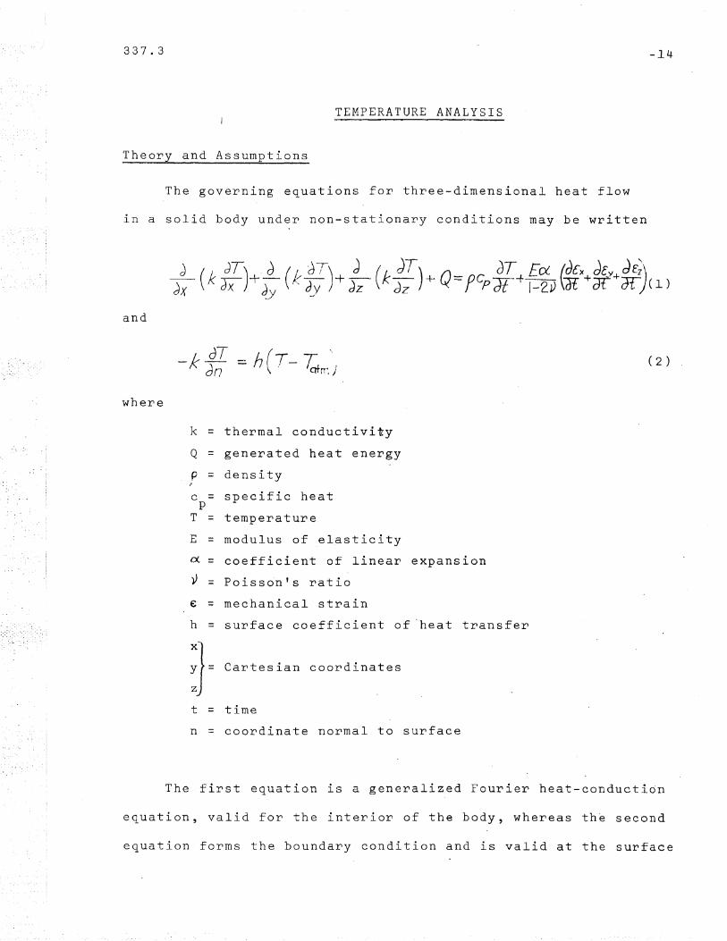
The governing equations for three-dimensional heat flow

in a solid body under non-stationary conditions may be written

-l4

and

( 2 )

where

k = thermal conductivity

Q = generated heat energy

p = density

c = specific heatp

T = temperature

E = modulus of elasticity

ex = coefficient of linear expansion

V = Poisso"n's ratio

€ = mechanical strain

h = surface coefficient of·heat transfer

~}= Cartesian coordinates

t = time

n = coordinate normal to surface

The first equation is a generalized Fourier heat-conduction

equation, valid for the interior of the body, whereas the second

equation forms the boundary condition and is valid at the surface

337.3 -15

of the body. In this study, coefficients generally were assumed

to be variable with temperature.

impossible, certain assumptions have to be made even in the case

While an analytical solution of this problem is pvactically

of numerical methods.

this analysis:

The following assumptions were made in

1. An initial temperature distribution in the rolled

member as well as the temperature of the atmosphere

surrounding the cooling shape are known.

2. The conditions are considered to be two-dimensional,

that is, the axial heat flow in the member is neglected.

(This assumption is justifiable with the exception of

regions close to the ends of the member.)

3. The member and the boundary conditions are symmetri­

cal about both axes of the cross-sectional plane.

4. The material is considered homogeneous and isotropic

throughout the cross section; the material coefficients

are known as functions of temperature.

5. The heat transfer conditions from the shape surface to

the atmosphere are known; no external or internal heat

source is acting during cooling.

Considering the assumptions which have been stated above the

subjected to cooling in the atmosphere (assumption 5) with no

sharp variations in the temperature-time history, the coupling

. (10 )effect of temperature and straln can be neglected. This

For a bodyfollowing simplifications of Eq. (1) can be made.

means that the second term of the right member of Eq. (1) is

337.3

negligible.

in the body.

Further, Q = a since there is no heat generated

Finally, from assumption 2 it follows that the

-l6

third derivative of the left member of Eq. (1) vanishes.

Equat·ion (1) now can be simplified to

Formulation of Finite-Difference Relationships

For a finite-difference solution the cross section must

( 3 )

be subdivided into a mesh, Fig. 5. The mesh spacing for H-shapes

was made variable in order to limit the number of mesh points. (13)

II JI

The common explicit finite-difference method used to solve

transient thermal flow problems is based on a representation of

the geometrical derivatives in Eq. (3) by finite central differ-

ences and of the time derivative by a finite forward difference.

This means that the unknown temperature

pressed in terms of the known temperatures ,can be ex-

)

T 'k\.+1) J) and at the previous time

interval. See Fig. 6a. However, a numerical stability criterion

is involved in this method, restricting the possible time interval

to

(valid for carbon steel) and

tJ. t ~ ~----.---I__-2tcp (~ + e&z)Substituting ~ ,--' 0.3 ft

2 /hrpC

I PI1x = l1y~0.005 ft into Eq. (4) gives L\t, ~ 0.1 sec. Thus for

337.3 -17

the subdivision chosen the time interval in the calculations

must be chosen to be less than 0.1 sec. This means that the

complete temperature field over the whole cross section must

be computed at least 600 times for each minute of the cooling

period. Narrow mesh spacings will lead to very tedious com-

putations, even when using a high speed computer.

on a

For this reason, another method was used which is based

principle developed by Peaceman and Rachford in 1955(11),

The principle, referred to as the implicit alternating direction

(IAD) method, is illustrated schematically in Fig. 6b. One of

the geometrical derivatives is always represented by a forward

difference and this derivative is taken in alternating directions.

It has been proven that the lAD method is stable for a rectang-

1 , , , d b' " 1 A (12)u ar lntegratlon reglon an an ar ltrary tlme lnterva ~t.

Numerical studies have shown that the method is stable for arbi-

trary time intervals also for more complex shapes of the integra-

tion region.

The detailed derivation of the finite-difference equations

for the interior and the boundary of the cross section in this

application of the lAD method is given in Ref. 2.

The calculation is started at the assumed initial state of

temperature. The temperature field after the first time interval

337.3 -18

is then computed, integrating in one direction of the cross

section. After the next time interval the temperature is com-

put e din th e other di re ct i'on and th e campu t at ion then continue s

following a step-by-step procedure and integrating in alternating

directions.

A finite-difference equation can be formulated for each

mesh point at a certain time interval. Since the number of un-

known temperatures is equal to the number of mesh points, the

problem can be solved provided the coefficients are known. The

equations for each time interval will form a number of compara-

systems can, therefore, be solved relatively easily.

equation system contains coefficients different from zero only in

The coefficient matrix to each

The equationthe diagonal and in the two adjacent disgonals.

tively simple equation systems.

Thermo-Physical Coefficients

The coefficients which enter Eqs. (2) and (3) are the thermal

conductivity k, the densitYf ' the specific heat c p ' and the sur-

face coefficient of heat transfer h. In the preceding sections

it was assumed that these coefficients were known. The means for

consideration of the actual thermo-physical properties were part

of the reported investigation but are discussed in detail else-

h(2,13)

were. The variation of properties with temperature was

included as well as the effect of phase transformations.

337.3 -19

Figures 7 through 9 show the variation of k, c , and h withp

temperature for carbon steels. Upper and lower bounds for test

data found in a literature survey(2) are indicated with dashed

curves in the diagrams.

used in the computations.

chosen for the density.

Solid curves represent the relationships

3A constant value of 4~O Ib/ft was

This gives a better approximation of the

h - 1 b h - h h f hI- bl d -t (2,13)P YSlca e aVlor t an t e use 0 t e actua , varla e enSl Y'

The discontinuity in c at 1200-1400~F is a result of thep

phase transformation~ austenite ~ ferrite + cementite. This was

dealt with in a manner different from earlier studies. (2~13,14,15,16)

The surface coefficient of heat transfer includes the effect

geometrical reduction factor was applied to h to take into account

the fact that the free heat transfer may be obstructed~ for instance,

In the computations aof convection, conduction and radiation.

on the inner surfaces of the flanges and on the web. This factor

was computed according to Lambert's cosine law for heat radiation.

A further reduction due to the external conditions during cooling

can be used in the computations, when applicable,

The material coefficients which enter the· computation of

the temperature field at a certain instant, t2n

+l

, (see Fig, 6b) are

the average values in the time int'erval between the previous time,

t 2n , and the time considered, t 2n+ l , Since only the temperatures

at t2n

are known at that moment, the coefficients can not be eval-

uated before the temperatures at t2

are calculated,n+l

337.3 -20

This complication was solved with an iterative method. As

a first guess the coefficients were evaluated from temperatures

which were extrapolated linearly in time from the previous and

the next to the previous .temperatures at the considered mesh point.

Approximate values for all coefficients could be obtained in this

way. Using the approximate coefficients, a preliminary temper-

ature field was calculated as described in the previous section.

With the preliminary temperature field, new improved values

for the criefficients were evaluated for the average of the previous

temperature and the computed preliminary temperature. Using these

improved values, the temperature field was calculated again.

The iteration may be continued to give any prescribed accuracy.

From numerical studies in the present application, it was found

that the error after one iteration, as described above, is negligible.

Results of Temperature Computations

A flow diagram of the computer program for temperature deter­

mination is shown in Fig. 10. The computations were carried out

in a computer type CDC 3600. The machine time "needed for a com­

plete computation including thermal stress calculation ranged from

about 1 to 3 minutes for a cooling period of 30 to 90 minutes.

Numerical studies of a specific case (same conditions as ~n

the computations shown in Fig. 11) indicated that while the

337.3 -21

ordinary explicit finite-difference method would require ap­

proximately 40,000 time intervals to be computed, the prescribed

accuracy could be obtained with 200 time intervals when using

the lAD method. Although the number of numerical operations in­

volved in each time interval of the lAD method is 10-20 times

that of the explicit method, it may be concluded that the lAD

method is far more efficient for these calculations.

The computed time-temperature curves for a European shape

'HE 200 B', approximately equivalent to the 8WF40, and using

average curves for the material coefficients, are shown in Fig.

11. Three different curves are given, corresponding to three

different locations in the cross section (that is, the temperature

in three out of the 71 mesh points used are shown). The initial

temperature was assumed to be 1830 0 F (IGaaOe), uniform through

the cross section. This temperature corresponds to, the average

temperature in practice at, or immediately before, the finish­

rolling.

In the beginning of the cooling the flange tips and the web

'point cool much faster than the point at the junction between

flange and web. When the coolest part reaches the phase trans­

formation temperature (~13400F), the cooling curves tend to level

out due to the transformation heat. After some time the trans­

formation is finished and the cooling curves then proceed with a

slope almost as if they were a continuation of the curves before

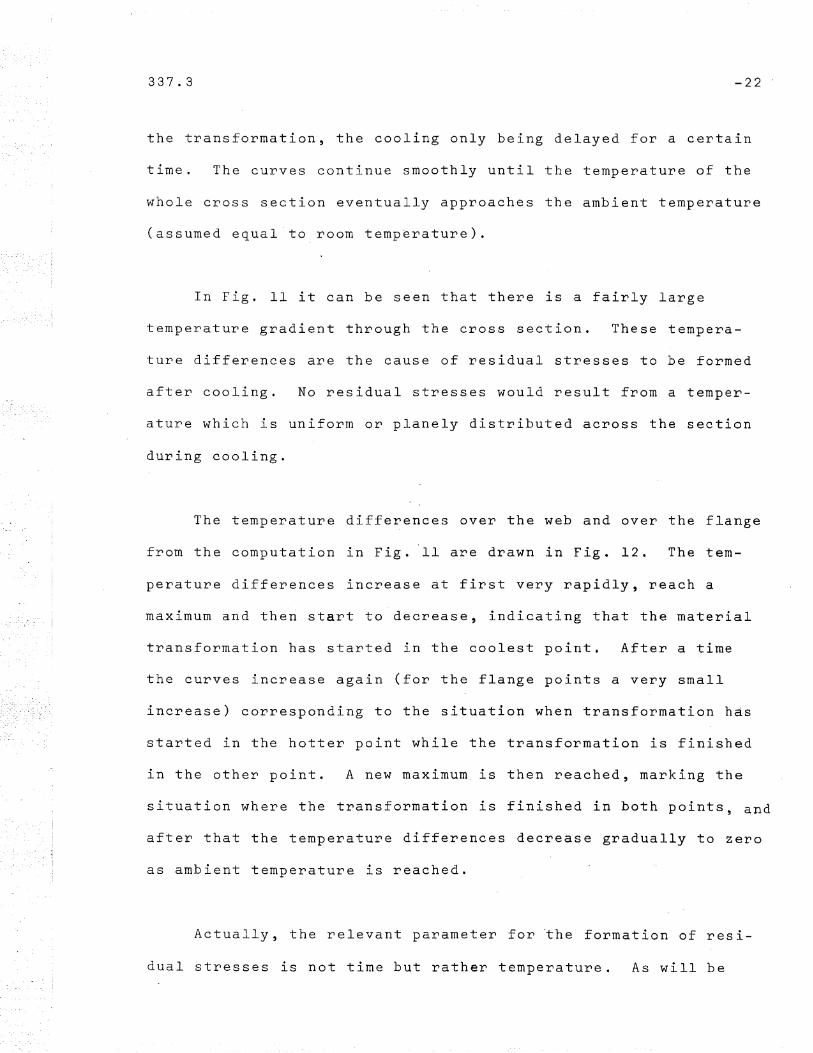
337.3 -22 .

the transformation~ the cooling only being delayed for a certain

time. The curves continue smoothly until the temperature of the

whole cross section eventually approaches the ambient temperature

(assumed equal"to room temperature).

In Fig. 11 it can be seen that there is a fairly large

temperature gradient through the cross section. These tempera­

ture differences are the cause of residual stresses to be formed

after cooling. No residual stresses would result from a temper­

ature which is uniform or planely distributed across the section

during cooling.

The temperature differences over the web and over

from the computation in Fig. "II are drawn in Fig. 12.

the flange

The tem-

perature differences increase at first very rapidly, reach a

maximum and then start to decrease~ indicating that the material

transformation has started in the coolest point. After a time

the curves increase again (for the flange points a very small

increase) corresponding to the situation when transformation has

started in the hotter point while the transformation is finished

in the other point. A new maximum is then reached, marking the

situation where the transformation is finished in both points, and

after that the temperature differences decrease gradually to zero

as ambient temperature is reached.

Actually~ the relevant parameter for "the formation of resi-

dual stresses is not time but rather temperature. As will be

337.3

shown later, the critical temperature differences are those

existing in the temperature region where the material changes

from perfectly plastic to elastic-plastic condition (see also

the discussion according to Ros). Therefore, the temperature

differences as a function of the temperature is the most apt

background for a discussion of residual stress formation. In

Fig. 13 has been redrawn the upper diagram of Fig. 12, but

with the temperature difference as a function of the tempera-

-23

ture in the web point. This diagram indicates that the effect

of the phase transformation is significant in a major portion

of the cooling process.

Computations of the same kind as those illustrated in

Figs. 11 through 13 were obtained for a large number of differ-

ent cases.

briefly:

The results of these computations may be summarized

the effect of the assumed initial temperature distri­

bution is negligible in the critical region (below the

transformation temperature) provided the assumed tem­

perature is chosen sufficiently high.

Small variations in the thermo-physical properties have

only a small influence upon the computed thermal behavior.

Shape geometry has a significant effect upon the absolute

temperature as well as the relative temperature state.

Cooling conditions can have a significant effect upon the

absolute and relative temperature state.

337.3

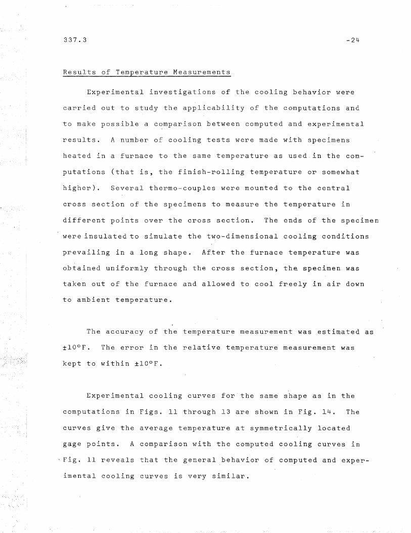
Results of Temperature Measurements

-24

Experimental investigations of the cooling behavior were

carried out to study the applicability of the computations and

to make possible a comparison between computed and experimental

results. A number of cooling tests were made with specimens

heated in a furnace to the same temperature as used.in the com­

putations (that is, the finish-rolling temperature or somewhat

higher). Several thermo-couples were mounted to the central

cross section of the specimens to measure the temperature in

different points over the cross section. The ends of the specimen

were insulated to simulate the two-dimensional .cooling conditions

prevailing in a long shape. Af~er the furnace temperature was

obtained uniformly through the cross section, the specimen was

taken out of the furnace and allowed to cool freely in air down

to ambient temperature.

The accuracy of the temperature measurement was estimated as

tlooF. The error in the relative temperature measurement was

kept to within ±looF.

Experimental c__ooling curves for the same shape as in the

computations in Figs. 11 through 13 are shown in Fig. 14. The

curves give the average temperature at symmetrically located

gage points. A comparison with the computed cooling curves in

~ Fig. 11 reveals that the general behavior of computed and· exper­

imental cooling curves is very similar.

337.3 -25

Figure 15 gives the results from repeated cooling tests

with the same specimen, now plotted in the form of temperature

difference as a function of.time. (The thermo-couple in the web

center became loose in one of the cooling tests so only three

curves are shown in the upper diagram). A comparison with the

computed results (dashed lines in Fig. 15, taken from Fig. 12)

-for this shape and based upon average material data from the

literature shows that the difference between computed and experi­

mental results is of the same order as the variation between re­

peated measurements.

In two of the tests, there was an unintentional axial heat

flow due to unsuitable insulation shields at the ends of the spec­

imen; the first test was accelerated and the second test delayed

due to the influence of the axial heat flow. However, the measured.

temperature differences were still at the same level as for the

other two tests.

In Figure 16 the upper diagram from Figure 15 has been redrawn,

now with temperature as a parameter. This diagram reveals the actual

similarity between the different test results and the computed re-

ther demonstrated in the following section.

suIts. The significance of this basis for comparison will be fur-

In conclusion, it may be stated that there is a fairly good

agreement between experimental results and the results computed

337.3

from average coefficient curves.

-26

Similar agreement was obtained

also from repeated tests on a different shape. Therefore, it

appears possible to compute the time-temperature history during

cooling with a reasonable accuracy, provided the actual cooling

conditions and the actual geometry are simulated in the comput~­

tion.

337.3 -27

THERMAL STRESS ANALYSIS

Theory and Assumptions

methods used for calculation of welding residual stresses can be

A number of methods for thermal stress analysis have been

Because of the complex conditions

A summary of some previous

presented in the literature.

certain assumptions must be made.

found in Ref. 17. As pointed out there, most previous methods

consider neither plastic deformations nor the actual equilibrium

conditions.

Solutions based on an analytical analysis for simple geometry

(11)and boundary conditions have been reported. However, for

more complex shapes and variable coefficients such solutions are

presently not developed. Other investigations which included

· bl ff·· (17,18) b d bvarla e cae lClents were ase upon a step- y-step

analysis· with a stepwi'se algebraic addition of the thermal stress

existing before the time interval considered and an incremental

stress formed during this time interval.

The model for the thermal stress formation as used in the

present investigation is different from the methods previously

mentioned. Before the method is discussed further in detail it

is pertinent to summarize the assumptions made in this study.

(1) The material is elastic-perfectly-plastic at all

temperatures.

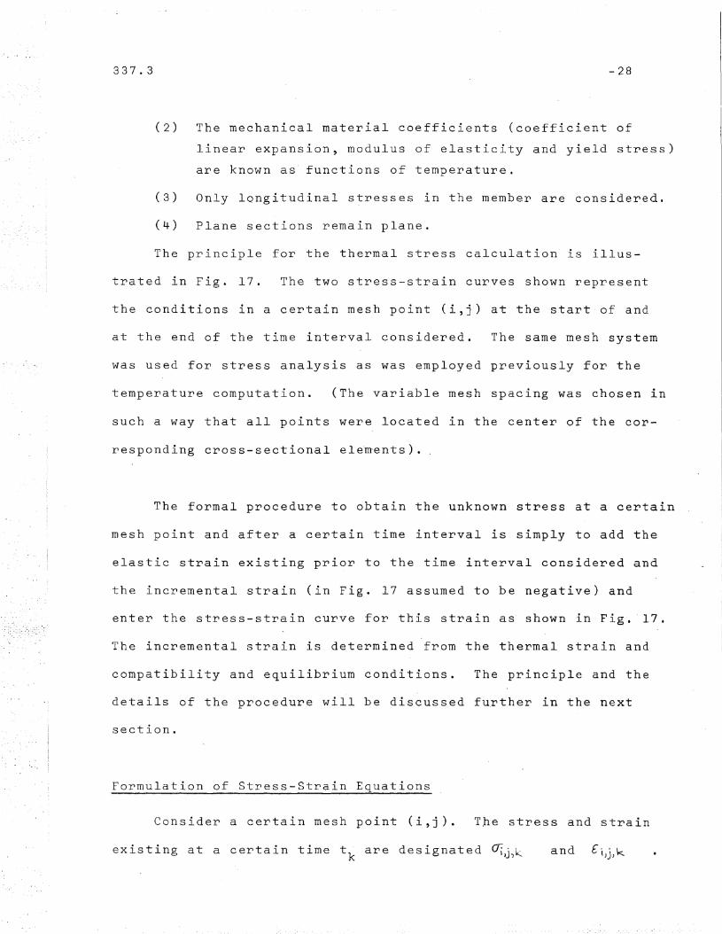
337.3 -28

(2) The mechanical material coefficients (coefficient of

linear expansion, modulus of elasticity and yield stress)

are known as' functions of temperature.

(.3) Only longitudinal s~resses in the m~rnber are considered.

(4) Plane sections remain plane.

The principle for the thermal stress calculation is illus-

trated in Fig. 17. The two stress-strain curves shown represent

the conditions in a certain mesh point (i,j) at the start of and

at the end of the time interval considered. The same mesh system

was used for stress analysis as was employed previously for the

temperature computation. (The variable mesh spacing was chosen in

such a way that all points were located in the center of the cor-

responding cross-sectional ele~ents)..

The formal procedure to obtain the unknown stress at a certain

mesh point and after a certain time interval is simply to add the

elastic strain existing prior to the time interval considered and

the incremental strain (in Fig. 17 assumed to be negative) and

enter the stress-strain curve for this strain as' shown in Fig. 17.

The incremental strain is determined from the thermal strain and

compatibility and equilibrium conditions. The principle and the

details of the procedure will be discussed further in the next

section.

Formulation of Stress-Strain Equations

Consider a certain mesh point (i,j). The stress and strain

existing at a certain time tk

are designated ~J)k and

337.3 -29

If, initially, the element is assumed to be cut free from the

other elements it will contract corresponding to a strain -C,EJ", ~-" •

, ~ K...

During the succeeding time interval the temperature is changed

from ~j)k to T·, .11_\ : ~.-~

For the free element this would cause

a thermal strain increment denoted by

calcuiated from the equation

which can be

( 10)

The strain resulting, that is, the free strain is ( _ c E . , ...L /'\ ~:-. I " \.

L 0, ' '/ ~ J--... v, 1 k;', ') L •lJ )y.., .).... ') . L./

Now suppose the elements are joined together again. Due to

the compatibility requirements the strain change in each element

Cmu s t tot a 1 a s t r a i n increm en t D. 6 i)j I k:t 1/2. whiehis dis t ribute d

ference between this imposed strain and the free strain is equal

to the s tra in aft er the time in terva 1 con·s idered

(11)

The dif-planely over the cross section (assumption 4 above).

The strain increment

cequal to (!::l.Ei,i)~.+i/2

"" "

11 £ i}j, k-t \/2

1). E: ~)j I k+ ;2.) •

in Fig. 17 is, therefore,

if

(12)

if

will give rise to a stress equalThe strain

to

If n denotes the number of mesh points, there are generally n

unknown strains f ...\ . ' ~ . and n unknown stresses

337.3 - 3 a

Furthermore, there are n strain increments which

can be represented by three unknowns, that is, a total of 2n+3

unknowns. Equation (11) gives one relation for each m~sh point

three equations to find a solution are obtained from the equili-

brium conditions, that is, one equation from the equilibrium of

and so does Eq. (12),' or together 2n equations. The rema.ining

force and two equations from the equilibrium of moments.

The formal addition of strains instead of stresses as in the

previous studiesJ17 ,18) is considered to fulfill the assumptions and

to simulate the physical behavior in a more correct way. A simplified

exa~ple will clarify the difference between the two procedures.

Consider a system as shown in Fig. l8a to be maintained at a constant

elevated temperature and loaded form zero to a certain stress below

the yield .point. The temperature is then allowed to cool·and at a

lower constant temperature the specimen is unloaded. The results

obtained with the two principles are shown in Fig. 18a. Since the

stress was assumed to be less than the yield point of the material,

the behavior must be purely elastic. The method based on an addition

of stresses .will result in an elastic st~ain re~aining after

unloading to zero stress which is mechanically impossible. The

general case illustrated in Fig. 18b the methods give two diyferent

stresses happen to give a negative stress fo~ a positive elastic

Here the addition of

In the moreother princ~ple will give zero strain after unloading.

answers for the stress being calculated.

strain, also mechanically impossible.

337.3 -31

From the discussion above it might be thought that the

methods will furnish results which are completely different.

However, comparative calculations carried out with both methods

have shown that the diffevence is vevy small, especially when

the variation in elastic modulus is small from one time interval

to another (that is, with short time intervals).

Figure 19 shows a short flow diagram of the computer program

used for the stress computation. This program was a subroutine

to the program for temperature determination.

Mechanical Coefficients

found in the literature for carbon steels as well as the curves

Figures 20, 21, and 23 give the upper and lower limits of data

It might be well to point out that the coefficient of linear

, the elastic modulus E, and the yield stress cry

normally is given as the average value in a certain

The properties of interest here are the coefficient of linear

expansion oL

expansion

temperature interval, ranging from room temperature to the con-

d .. h" .. (2)use lD t e lnvestlgatlon .

sidered temperature. Therefore, the thermal elongation from a

temperature change between two temperatures must be computed from

an equation of the type shown in Eq. (10).

The variation in ~ between different carbon steels is rela-

tively small. The behavior in the transformation temperature

337.3

range is due to the gradual transformation tI-.cx which is ac-

-32

companied by a volume expansion. The temperature at the two

discontinuity points from tests on different materials generally

coincides with the A3

and Al temperatures for the actual carbon

contents.

The elastic modulus is normally measured by a dynamic method

to minimize the effect of time-dependent influences due to creep.

Figure 21 co-ntains both "static" and "dynamic" measurements. The

variation is reasonably small.

It is noted that a good representation of the actual non­

linear stress-strain relationships at- different temperatures and

for the strain range of interest in the present application was

obtained when the yield stress of the elastic-perfeCTly-plastic

model equals the 0.2% proof stress. A comparison between the

actual stress-strain relationships and the elastic-perfectly­

plastic relationship based on a yield level equal to cr 0.2' is ex­

emplified in Fig. 22. Fortunately, 00.2 is the stress level­

normally reported in the literature to represent the yield paint

at higher ~emperatures. Upper and lower limits of data from the

literature are given in Fig. 23.

While t'ime- dependent deformat ions have no significant inf lu­

ence on the IT O. 2 stress level at temperatures below 700-800 o F,

this is not true for higher temperatures. Results of some creep

tests are sketched in Fig. 2-3. The applicable stress-strain re-

lationship will fall between the two limits of data obtained from

337.3 -33

tensile tests and creep tests. It should however be noted that

the duration of the creep tests is as compared to a few

minutes for the critical temperature range in the cooling process

of most rolled shapes. Furthermore, the creep tests results were

obtained at a constant load. However, in the application studied

the stress varies and the conditions at high temperatures are in-

between the creep case and the relaxation case where strain is kept

constant. While it is possible for a tensile test specimen to sus-

· d d· · · (20)taln a loa un er contlTIUOUS recrystalllsatlon ,zero stress

would result in a relaxation test.

Approximate considerations of the time-dependent effects and

the difference in behavior at constant stress versus constant strain

have led to the curves shown in Fig. 23.

Results of Thermal Stress Computations on Plates

Figure 24 shows an example of the computed temperature and

thermal stress behavior during cooling of a plate 24" x 3t". It

was assumed that the initial temperature was 18300F (IOaaOe),

uniform through the cross section, and that the surface heat trans-

fer was free in all directions.

plastic condition, denoted by the shaded area in the first diagram

At the temperature of 1830oF, the material is in perfectly

The remaining diagrams show curves for constant tem-

perature and constant stress at 10, 20, 30, and 40 minutes and

of Fig. 24.

337.3

finally, at a very long time after the initial state.

-34

After 10 minutes the temperature has cooled to about 1300 ­

1500 o F. The temperature is still too high to allow any stresses

to be developed (Fig. 23). After 20 minutes of cooling the

temperature ranges from about 1150 - 1350 o F, the plate edges

cooling faster than the interior of the plate. At this moment

,the coolest parts have entered the elastic region, but the

stresses are negligible. After another 10 minutes, the tempera­

tures being approx. lOOO-1250 o F, the cross section still is partly

in the plastic condition although the location of the plastic

region is different from that obtained at t = 20 minutes. This is

due to the effects of the phase'transformation.

At t = 40 minutes the temperature is about 950 - IIOGor and

the entire corss section is elastic. When cooling further to

ambient temperature, the thermal contraction of the central hot

portion would be greater tha~ that of the cooler surface parts.

However, due to the symmetry the compatibility conditions require

that the contraction is equal throughout the cross section. This

will introduce tensile stresses in the central portion, balanced

by compressive stresses in the regions which were cooling faster.

The resulting residual stress distribution after cooling to ambient

temperature is shown in the last diagram of Fig. 24. In this case

the temperature differences through the cross. section were large

enough to cause compressive residual stresses at the yield

point at the edges of the plate (shaded in the diagram). The

337.3 -35

results exemplify the rule of thumb that the portions of the cross

section to cool faster will be left in a state of compressive

residual stress.

Figures 25 through 28 give the results obtained for four

different plate sizes: 6" xi", 20" X Itt, 12 t1 X 2 t1, and 24" x 3t".

Three curves are shown for each plate: the distribution of resi-

dual stress in the plate surface, in the mid-plane, and the aver­

age across the thickness. "The four different plates represent

two thin plates (less than, or equal to, 1 inch) and two thick

It can also be noted from a comparison of the data in the

diagrams, that there is a trend of increasing magnitude of the

the thickness is less than 3 ksi, whereas the same variation in

the thickest plate (S! inches) is approx. 15 ksi.

plates. In the tit plate (Fig. 25) the maximum variation across

stresses with increasing size of the plates. The average residual

stress at the plate edge is -10, -13, -21, and -31 ksi, respec­

tively, and the average tensile stress in the center of the plates

is approx. 3, 2, 8, and 9 ksi, respectively, for plates of in­

creasing size.

The distribution of residual stress through the thickness

is generally close to a parabolic shape. The distribution across

the width is of a similar shape, and colser to a parabola with

smaller width/thickness ratios.

337.3 -36

For increasing thickness of the plate, the magnitude of

residual stresses at both center and edge will increase as well

as the extension of the compressive stress region into the plate.

This is illustrated in Fig. 2"9. The influence of plate width

on the residual stress distribution is more complex as shown in

Fig. 30.

alized.

Note that the dimension of width is shown non-dimension-

In actual scale, the extension of the compressive stresses

in a wide plate is larger than in a smaller plate. Finally, the

effect of th'e "size factor", when keeping the width/thickness ratio

constant, is indicated in Fig. 31. The difference in the center

part of the diagram are very small in this specific case, the de-

viation being less than I ksi, "whereas the stress magnitude in the

ar~a close to the edges is a function·of the plate size.

Results of Thermal Stress Computations on H-Shapes

Figure 32 shows an example of the computed temperature and

thermal stress behavior during cooling of a shape HE 200 B. (Com-

pare with Figs. 11 through 13). The initial temperature was assumed

to be 1830oF, uniform over the cross section. The material is in

the perfectly plastic condition, denoted by the shaded area in the

first diagram of Fig. 32. The succeeding diagrams show contour

lines for equal temperature and equal stress at 2, 4, 8, 16 minutes

the temperature ranging roughly between 1250' and 1350 o F, the coo1-

2 minutes the temperature has cooled down.to about 1400-l525 0 F,

After

After 4 minutes ~f cooling,

est parts, that" is the flange tips and the web, have entered the)

but still no stresses have been formed.

and finally, at a very long time after the initial state.

337.3

elastic condition. The stresses are still negligible.

-37

After

another 4 minutes the entire cross section is elastic and re­

mains so for the rest of the cooling. The sign of the s~resses

at 8 minutes reflects the fact that the temperature differences

through the section have increased from t = 4 min to t = 8 min.

This is due to the phase transformation; see Fig. 12. At 16 min

from the initial stage, the temperature gradients have decreased,

giving increased stress gradients. Finally, after a very long

time the ambient temperature is approached and the thermal stress

distribution is then equal to the residual stress distribution.

The parts to cool fastest, that is, the flange tips and the web,

are left with a compressive residual stress which is balanced by

tensile residual stresses at the junction between flange and web.

A comparison between the residual stress diagram and the tem~

peratur~ diagram in the range where the material changes from the

plastic to the elastic-plastic condition reveals a similarity be­

tween these patterns. Figure 33 illustrates this further. The

thermal stress for three points of the cross section is compared

with the corresponding yield stress, with t~me as a parameter.

It is noted that the thermal stresses are elastic except for

a short interval in the beginning of the cooling~ Thi,s can be

observed in Figs. 24, 32, and 33. The change of the material from

the plastic to the elastic-plastic condition is a function of tem­

perature. These )facts imply that the temperature differences at

the time when this particular temperature region is passed are of

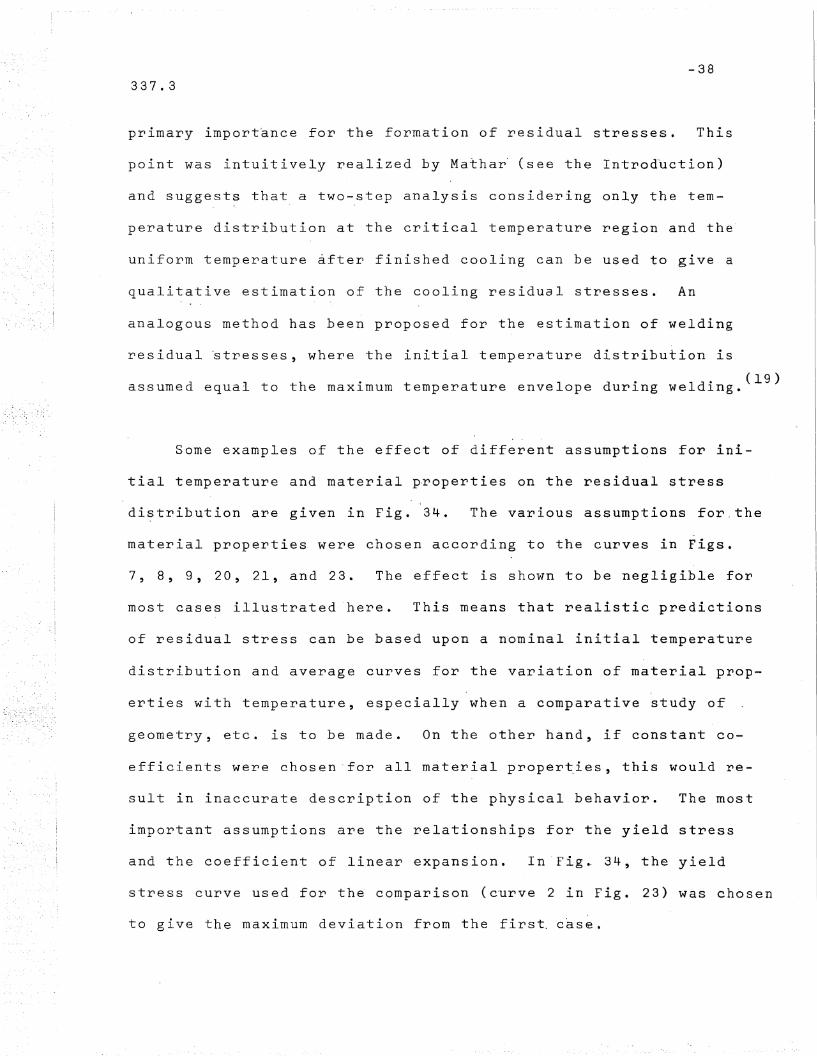
-38337.3

primary importance for the formation of residual stresses. This

point was intuitively realized by Mathar" (see the Introdtiction)

and suggest~ that a two-.step analysis considering only the tem-

perature distribution at the critical temperature region and the

uniform temperature ~fter finished cooling can be used to give a

qualitative estimation of the cooling residual stresses. An

analogous method has been proposed for the estimation of welding

residual 'stresses, where the initial temperature distribution is

d 1 h · 1 d· ld· (19)assume equa' to t e maX1IDum temperature enve ope urlng we lng.

Some examples of the effect of different assumptions for ini-

tial temperature and material ~roperties on the residual stress

of residual stress can be based upon a nominal initial temperature

material properties were chosen according to the curves in Figs.

distribution are given in Fig. 34. The various assumptions for. the

This means that realistic predictions

The effect is shown to be negligible for7, 8, 9, 20, 21, and 23.

most cases illustrated here.

distribution and average curves for the variation of material prop-

erties with temperature, especially when a comparative study of

geometry, etc. is to be made. On the other hand, if constant co-

efficients were chosen-for all material proper~ies, this would re-

important assumptions are the relationships for the yield stress

stress curve used for th~ comparison (curve 2 in Fig. 23) was chosen

In·Fig~ 34, the yield

The most

and the coefficient of linear expansion.

suIt in inaccurate description of the physical behavior.

to give the maximum deviation from the first. case.

-39337.3

Figure 35 illustrates the results obtained for two shapes

which are geometrically similar, one being the shape HE 200 B,

the other, a hypothetical shape with dimensions twice those of the

HE 200 B. All other variables are exactly the same. Figure 36

gives another comparison between an HE 200 B shape and a shape

of the same dimensions except that the width was 4" instead of

8". The results show that the dimensions and the size of the shape

is a significant variable.

So far it was assumed that the heat transfer is free in all

directions .. Figures 37 and 38 give examples of the possible in­

fluence of different cooling conditions on the residual stress

distribution.

In the first case (Fig. 37) the heat transfer from the web

surfaces was reduced to a certain percentage varying between 100

and 30%. This will simulate very schematically the conditions

when the shape is placed with the web in vertical position during

cooling and with adjacent shapes reducing the possible heat trans­

fer. The results show that the distribution in the web is com­

pletely reversed as compared to the distribution to be expected

from free cooling. Instead of compressive stresses in the central

part of the web, there are high tensile stresses. The type of dis­

tribution obtained in the flange is similar for both cases although

the position of the zero line in the forced heat-transfer case has

shifted, resulting in higher compressive stresses to balance the

tensile stresses in the web.

337.3 -40

Residual stress distributions of this forced heat-transfer

type have been measured in some cases; for instance, see the

distribution obtained by Mathar, Fig. 4. The H-shapes of Figs.

37 and 4 are very similar, and the residual stress distributions

exhibit a good ~esemblance.

Figure 38 illustrates further the effect of various cooling

conditions~ Results were obtained for three different assumed

heat-transfer conditions: free heat transfer, heat transfer re-

duced by 50% .on all surfaces except the outer sides of the flanges,

and finally heat transfer reduced by 50% only on these outer flange

surfaces. Schematically, the three different cases can be consid­

ered simUlating different arrangements during the cooling, that is,

a member cooling separately, a member cooling with the web in a

vertical position and adjacent members on both' sides, and a member

cooling with the web in a horizontal position and adjacent members

on both sides. As can be seen in Fig. 38, the residual stress

distribution in the web is v~ry sensitive to the cooling conditions.

Stresses in the flange are also different for the three cases

although the stresses at the flange tips are all at the same level.

It is expected that the extreme cases illustrated in Figs. 37

and 38 represent limit conditions for normal manufacturing practice

of small to medium-size shapes. For prediction of the behavior of

most such shapes the assumption of free heat transfer appears reason­

able since a main part of the critical temperature range Is passed

before the shape arrives to the cooling bed. For heavy s~apes,

337.3 -41

however, the actual cooling conditions must be considered for

accurate predictions.

While the variation of residual stress across the thickness

is very small for thin components of the shape, this is not true

Figures 39 and 40 give the computed residualfor heavy shapes.

stress distribution for a heavy rolled shape 14WF426. The diagrams

shown are based on the assumptions of free cooling and reduced heat

transfer from the inner surfaces (the same assumptions as cases a

and b, Fig. 38). The variation through the thickness of the flanges

is quite considerable. Also, the stresses are higher than was en-

countered in the calculations for smaller shapes.

The heaviest shape rolled in today's practice is a "jumbo"

shape 14WF730. Figures 41 and 42 illustrate the distribution of

upon the same assumptions as in Figs. 39 and 40, that is, free

residual stresses in this shape, as obtained in computations based

cooling, and reduced heat transfer, respectively. The computed

stresses in the jumbo shape are very high in both cases considered,

and equal the yield stress in the outer portions of the flanges.

While the magnitude and distribution of residual stresses in

general plays a role, the residual stresses at the flange tips are

of primary importance in determining the buckling strength of cen­

( 9 )trally loaded compressed members. It is evident that the high

compressive stresses predicted in the heavy columns would be detri-

mental to column strength. Figure 43 shows computed column curves,

337.3 -42

based upon the tangent modulus load concept and the actual distri-

bution of predicted residual stresses for a 14WF730 shape. Figure

44 gives a comparison between the tangent modulus load and the

ultimate strength, both curve"s computed for weak axis buckling

and the free heat transfer type of residual stress (Fig. 41). The

ultimate strength curve was obtained assuming the initial out-of-

straightness to be a sine curve- with a mid-height deflection of

. .O.OOlL. Also shown in Fig. 44 is the Basic Column Curve developed

(21)by the Column Research Council from research on small rolled shapes.

The column curves based upon the predicted thermal residual stresses

in the 14WF730 fall far below the Basic Column Curve. However, in

the practical range of slenderness ratios of such heavy columns in

buildings, that is, at KL/r = 20 to 50, the reduction in strength

is not as severe as for slender columns.

The compressive residual stress at the flange tips obtained

in a number of computations" is plotted in Fig. 45 against a geo­

metrical parameter ~;:. This parameter had been suggested to des­

cribe the variation of measured residual stresses at the flange tips

. (7 8)of dlfferent shapes. ' The computations shown in Fig. 45 were

obtained from a systematic variatioTI_ of the four dimensions of the

shape, and assuming free heat transfer.

The results of these computations show a clear tendency of

increasing residual stress with increa~ing value of the parameter.

This was also noted previously from the experimental results.(7)

In Fig. 45 there appears to be a wide scatter, and the scatter was

337.3

still larger in the experimental values.

-43

A closer examination of

the points in Fig. 45 would, however, reveal that there is a reg-

ular pattern in that the upper points are for the heavier shapes

and the lower points are for lighter shapes.

From the computations plotted in Fig. 45 and from a consider-

b 1 b f rl -.J" 1 · ( 2 ) · · d h 11_a e num er 0 auQltlona computatlons It was notlce t at a

calculations furnished results in a region within two limiting

boundary lines and that most heavy shapes will fall in the upper

'part of this region and most small shapes in the lower part.

has been illustrated in Fig. 46.

Comparison With Experimental Results

This

While it can not be expected that all experimental results

will correlate well with computations based on nominal shape

dimensions, average material properties and certain assumptions

on the heat transfer in cooling, some comparisons between com-

puted and measured residual stresses will be made here to give an

idea of the applicability of the method. The experimental results

were obtained from the literature as referred to for each specimen.

The di~grams shown are for average residual stress through thick-

ness, except for the l4WF730 shape.

Figure 47 shows comparisons between experimental and computed

residual stresses in universal-mill plates of three different sizes,

337.3

6" X itt, 10" X ~", and 20" xl".

-44

The computed distributions

were obtained using the free heat-transfer assumption. For the

larger plate there are results of two independent measurements

- .. ' ( 2 2 2 3,)on different speclmens. ' The agreement between experimental

and theoretical results is satisfactory, ,the maximum deviation

being of the same order as the experimental ~ccuracy, except for

one of the 20" x 1" plates.

Figures 48 through 55 give some examples of the correlation

between experimentally obtained residual stresses and computed

results for shapes ranging from a small I-shape IPE200 to a

14WF730 shape. All computatioris were based on the free heat-

transfer assumption, except fo~ the l4WF426 shape, Fig. 54, where

comparative results are given based on the alternative assumption

of reduced heat transfer from inner surfaces of the shapes.

It should be borne in mind that the computations can simulate

only the "average" behavior. For the small and medium-size shapes,

computations based on the free- heat-transfer assumption appear td

predict the actual measured residual stress distribution fairly

well as could be expected (see the discussion on heat transfer in

stress in the center of the web approaches the yield point of the

In deep shapes the magnitude of the residualthe previous section).

material (assumed as 31 ksi in the comput~tions)~ Since the yield

stress of the web material in the deep test shapes apparently was

higher than the value assumed in the computations, closer correlation

337.3 - 45

would be obtained for these shapes applying the actual yield

stress level.

For the 14WF426 shape (Fig. 54) the seemingly crude assump-

tioD of forced heat transfer indeed predicts the residual stresses

better than the free-cooling assumption, most experimental points

falling in between the two calculated distributions and closer to

the solution based on the forced heat-transfer assumption. As

was stated earlier, detailed agreement for a heavy shape specimen

can be obtained only if the actual cooling conditions are known

and applied in the calculation.

l4WF730 shape shows little resemblance to the thermal residual

the left part of the measured diagram is qualitatively similar to

In Fig. 55, the measured residual stress distribution in the

Further studies

While the distribution in

The mill scale of the test specimen

stress distribution that was predicted.

the predicted distribution, the right part is completely different.

showed clear evidence of cold-bending yield lines.

after cooling in the mill.

It is believed that this id due to the cold-straightening operations

would be needed to determine the general significance of either

type of distribution in "jumbo" shapes manufactured according to

today's practice. However, as for the strength of the columns in

the lower slenderness ratios, the measured residual stress distribution

of Fig. 55 appears to be as unfavorable as the predicted thermal

d · -b - (27)stress lstrl utlon.

337.3

SUMMARY AND CONCLUSIONS

-46

The investigation described in the paper has been concerned

with the thermal. residual str~sses existing in hot-rolled plates

and H-shapes after cooling. A method was developed to calculate

these particular stresses considering the complete temperature

and stress history during cooling. The temperature calculation

is based on a solution of the Fourier heat conduction equation,

taking into ~ccount the actual boundary conditions at the surface

of the shape. The thermal stress is computed from the temperature

·distribution throughout the cooling process using an elastic­

perfectly-plastic model for the material behavior. The final the~mal

stresses after cooling ·to a~bient_temperature are the residual

stresses.

Calculations were carried out using a finite-difference method

and an electronic computer and simulating the actual conditions, in­

cluding variable material coefficients. The principal objective

was to investigate the influence of·different factors on residual

stresses. At the same time, a better understanding of the forma-

tion of cooling residual stress was achieved. The method can be

employed for prediction of thermal residual stresses in rolled

plates and H-shapes.

The results of the computations indicate that small variations

in the material coefficients have generally only a small 'influence

on the computed residual stress; the yield stress in the temperature

337.3 -47

range where this stress is small and approaches zero is the most

important material property in this respect. For calculations

with an accuracy which is satisfactory for most practical pur-

poses it is sufficient to base the computations on average curves for

the different coefficients and the actual type of material. Upper

and lower limits of data found in a literature survey for carbon

steels, as well a3 the average curves for these coefficients as

used in the study are given in the paper. Computations employing

constant coefficients for all relevant material properties will

give only a qualitative description of the actual temperature and

thermal stress behavior.

ing will occur during the conveyance of the shape from the finishing

stand to the cooling bed. The assumption of free cooling appears

to be reasonable for the conditions during the transport to the

The principal factors which influence the distribution

and magnitude of thermal residual stresses are 'shape geometry and

cooling conditions. A few cases of different assumed cooling con­

ditions were studied. It was found that the residual stress dis­

tribution in the web is extremely sensitive to the cooling condi­

tions. This may explain the apparantly erratic results for the

web obtained in experimental residual stress measurements'by dif­

ferent investigators. The distribution in the flange is less de­

pendent but the magnitude varies to a certain extent. The computa­

tions also indicate that the conditions on the cooling bed will

have a major influence in the critical temperature range only for

relatively heavy shapes. For small shapes a main part of the cool-

337.3 -48

cooling bed and consequently, this assumption should generally

result in good predictions for at least small shapes. For large

·shapes the free-cooling assumption mayor may not give valid

results, and for an accurate prediction the actual cooling

conditions on the cooling bed should be considered.

Se v,eral camp uta t ions were carr ie d out for pIa t e sand H­

shapes with a systematic variation of the dimensions as well as

for a number of commercially available H-shapes. These

computations were based on the free-cooling assumption. Practically

all computations for shapes resulted in a residual stress

distribution with compression at the flange tips and in the web,

and tension at the junction between flange and web. Correspondingly,

the edges of the UM plates are in compression, balanced by

tension in the center. However, the stress magnitude varies consid-

erably between different cross sections. The variation of computed

residual stress through the-thickness direction is negligible for

very thin elements, but for thick elements is almost as pronounced

as across the width direction.

One of the important details of the residual stress

distribution in an ,H-shape.d member under comp'ress.ive' load. is the

residual stress region at the flange tips. The computed

residual stress at the flange tip for all H-shapes considered

ranged between -0.7 and -31 ksi in compression, corresponding to

337.3 -49

showed the same general relationship between residual stress and

2 and 100% respectively of the assumed yield stress at room

parameter, relating the width to thickness ratio of the flange

Th . bit ·18 parameter, d/w' was suggested prevlously

There is a clear trend of increasing stress at the

and web components.

temperature.

from results of experimental. residual stress measurements, which

flange tips of H-shapes with increasing value of a geometric

the parameter.

It was also noted in the study reported in this paper

that there is a tendency of increasing magnitude of the residual

stresses with increasing size of the member. This is an important

~ained in previous research on small rolled shapes would not be

detrimentally affected by these high residual stresses, and more

conClusion, implying that the column strength characteristics ob-

Sim-

The column strength of a heavy rolled shape is

so than smaller rolled shapes with smaller residual stresses.

completely applicabl~ to the ,heaviest shapes rolled today. For

thick universal-mill plates and heavy sh~pes, the magnitude of

the predicted residual stresses is very high and can approach the

yield stress.

ilarly, for a welded H-shape built up of thick universal-mill plates,

the high compressive stresses at the plate edges would lower the

column strength.

The computed temperature distribution during cooling and

the computed residual stresses were compared with experimental

337.3 -50

results. The agreement between computed and experimental data

is good in most cases, indicating that predictions with reason­

able accuracy can be obtained using the analysis developed.

Future research topics concerning residual stresses in hot­

rolled plates and shapes could include an experimental study of

residual stresses applying statistical sampling methods. Some

hypotheses could be formulated with the information from this in­

vestigation. Further studies should be directed towards the pos­

sibility of reducing thermal residual stresses by rational manu­

facturing techniques. Controlled cooling procedures and cold­

straightening operations should prove useful in this respect.

The method as described in th~s paper was applied to members

cooling in the atmosphere. The computer program can be utilized

also for predicting residual stresses which are the result of dif­

ferent thermal treatments, for instance, the tempering process

employed for ASTM A5l4 steel sections. Analogous analyses can also

be used for studies of temperatures and residual stresses in flame­

cutting and welding. The use 9f finite-difference methods provides

a possibility of making realistic assumption~ tin the ,geometry, the

actual arrangement of heat sources, the boundary conditions, and

the material properties.

337.3

ACKNOWLEDGMENTS

-51

The study reported in this paper was a phase of an inves­

tigation into residual stresses and their influence on the strength

of structural elements; this investigation was carried out at the

Institution of Structural Engineering and Bridge Building at the

Royal Institute of Technology, Stockholm, Sweden. The investigation

was conducted under the sponsorship of the Swedish Technical Re­

search Council. The author is greatly indebted to Dr. Georg Wastlund,

Head of the Institution of Structural Engineering and Bridge Building,

for his continuing encouragement and constructive criticism during

the progress of the work. Mrs. Nan Straat and Mr. Toivo Tagel assis­

ted in the preparation of the computer programs for H-shapes and

plates, respectively. Their cooperation is gratefUlly acknowledged.

Dr. Bertil Aronsson, the Swedish Institute for Metal Research, re­

vie~ed the original dissertation and his suggestions were incbrporated

in the paper.

Certain aspects of the study were continued at Fritz Engineering

Laboratory, Lehigh University, Bethlehem, Pennsylvania, under a

general research project "Residual Stresses in Thick Welded Plates",

sponsored by the National Science Foundation. Dr. Lynn S. Beedle,

Director of Fritz Engineering Laboratory, encouraged the international

cooperative nature of the study. Dr. Lambert Tall, Principal Inves­

tigator of the research project at Lehigh University, reviewed the

paper and made a number of valuable suggestions. His interest and

encouragement in its preparation is sincerely appreciated. This

337.3 -52

research is under the technical guidance of Column Research

Council Task Group 1, of which Mr. John A. Gilligan is

Chairman.

Special thanks are also due to Miss Joanne Mies for

typing the report and to Mrs. Sharon Balogh for preparing

the drawings.

337.3

NOMENCLATURE

-53

Symbols and Units

A = area

E = modulus of elasticity

L = length

p = load

Q = generated heat energy

T = temperature

(ksi)

(in)

(kips)

(Btu/ft 3 -hr)

(OF)

b = width (in)

c = specific heat (Btu/lb-OP)p

d = depth (in)

H = surface coefficient of heat transfer (Btu/ft 2 -h-OF)

k = thermal conductivity (Btu/hr-OP-ft)

n = coordinate normal to surface (in)

r = radius of gyration (in)

t = time; flange thickness (hr; in)

w = web thickness (in)

x (in)

y = Cartesian coordinates (in)

z (in)

E

= coefficient of linear expansion

= strain

= Poisson's ratio

337.3 -54

.-

f density.-, =

(T = stress

( Ib / ft 3 )

(ksi)

Superscripts:

Subscripts:

C = compressive

R = residual

atm = atmosphere

cr = critical

f = flange

i = mesh point in x direction

j = mesh point in y direction

k = order of time interval

w = web

x = Cartesian coordinate

y = Cartesian coordinate; yield

z = Cartesian coordinate

= compatibility

= elastic

= plastic

= thermal

C

E

P

T

337.3

FIGURES

-55

..

FINISHING,TIONS

BLOOMING MILLI

r OPERA

I -,r---- HEATING

II

~ FURNACE

,. GAG -

-----

ROUGHINGPRESS ~

I-

STANDS

-I

COLD

"

STRAIGHTENING.........

INTERMEDIATEI ROLLS -

STANDS

-

r -FINISHING

I

_r HOT SA 1I

STAND- COOLING

_JL WJ ----- BED ------

-

Fig. 1 Schematic arrangement of a typical mill for

rolling structural shapesI

(Jl

0)

Fig. 2

-57

Rolling of a structural H-shape (Courtesy Bethlehem

Steel Corporation)

-58

8

l

Fig. 3

{Ute At +uw·Aw=Q

CTf- CTW=E a ~T

Predicted residual stresses in a hot-rolled H-shape.

After Ros(3).

-59

DIP 20 (~8W-40) A

Specimen No.1

STRESS 30IN WEB 20(KSI) 10

o 0 10 15 20(FT)

(0)

(KSI) ~~g~

DIP 20

(KSI) -Ig~-20~ "

(b )

Fig. 4 Measured residual stresses in a hot-rolled H-shape

DIP20 (nearest American equivalent 8WF40). After

Mathar(4) .

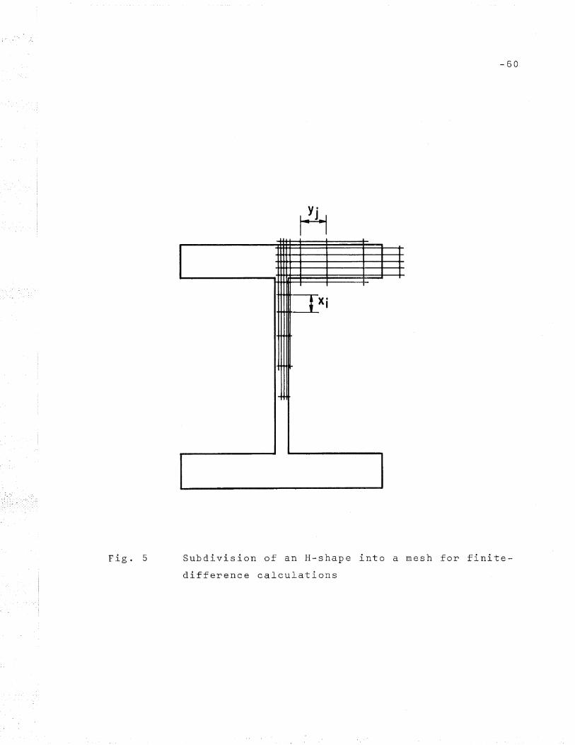
Fig. 5

-60

=rXj

...

Subdivision of an H-shape into a mesh for finite­

difference calculations

TIME

Fig. 6

-61

TIME

EXPLICIT FINITE- DIFFERENCE METHOD

(0 )

tI

Ti,j-I,k

IMPLICIT ALTERNATING DIRECTION (lAD) METHOD

(b)

Principles of finite-difference methods for the

solution of the Fourier Equation

50

--....... ......,

I

Lower Limit of Data

----.... 2·J -- rl"'t . ' 'c::: uc:::

10

20

30

40~' "" " " " [upper Limit of Data

'-- r-Functions Used..........

THERMALCONDUCTIVITYk (Btu/hr-OF-ft)

o 400 800 1200 1600TEMPERATURE (OF)

2000 2400

Fig. 7 Thermal conductivity k of carbon steels I())

tv

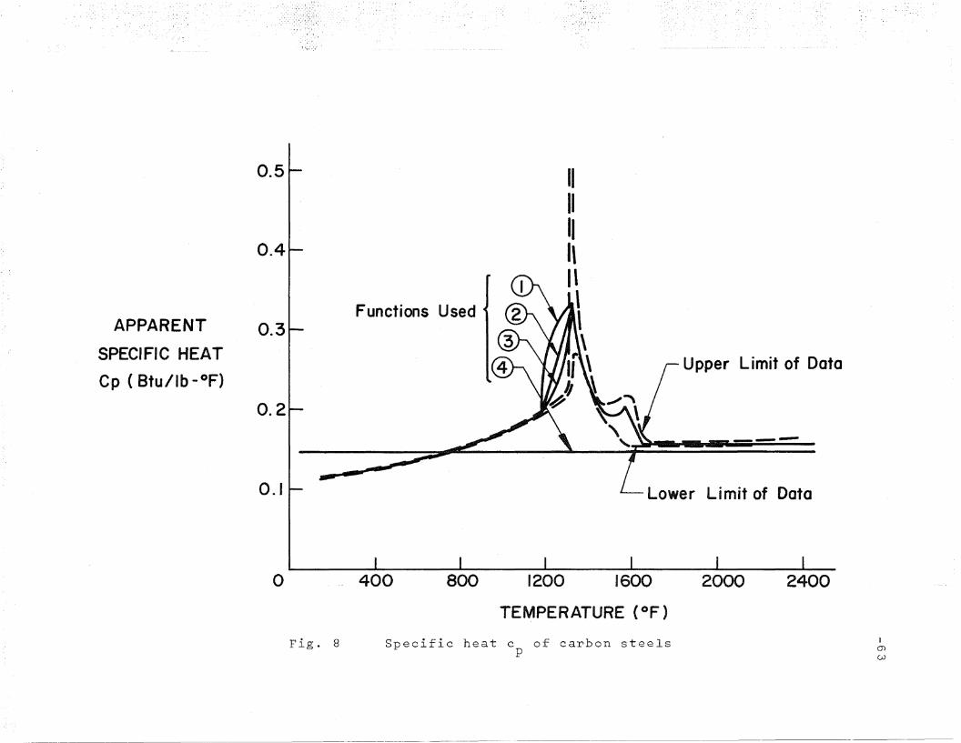
0.5

0.4

APPARENT 0.3

SPECIFIC HEAT

Cp ( Btu/lb -OF)

0.2

0.1

Functions Used

Upper Limit of Data

---Limit of Doto

o 400 800 1200 1600 2000

TEMPERATURE (OF)

2400

Fig. 8 Specific heat c of carbon steelsp

IQ)

w

-64

1.0THERMAL

EMISSIVITY 0.5

o

50

40

SURFACE COEFF.OF HEAT TRANSFER 30h (Btu / Ft2~Hr-OF)

20

10

Upper Limit of DataLower Limit of Data

400 800 1200 1600 2000 2400TEMPERATURE (OF)

(0)

FunctionsUsed

(Tota I).

Fig. 9

o 400 800 1200 1600 2000 2400TEMPERATURE (OF)

(b)

Surface coefficient of heat transfer h for

carbon steels

-65

1. READ DIMENSIONS, INITIAL CONDITIONS, TEMP. OF ATMOSPHERE, TIME SUBDIV.

2. COMPUTE GEOMETRIC SUBDIVISION, GEOMETRIC COEFF. OF SURFACE HEAT TRANSFER

3. PRINT INITIAL DATA, COMPUTED SUBDIVISION AND COEFFICIENTS

4. INITIALIZE k (k=O)

11. ISDIFFERENCE

(7j,J,k+1 - 71,'j , k~l)NEGLIGIBLE?

NO

COMPUTE NEW MATRIX COEFF. OF THE EQUATION SYSTEMS FOR ODD TIME STEPS

SOLVET HE E QUA T ION SYSTEMS, GI VI NG A NEW TEM PERA TURE SOL UTI 0 N n,j. k+1

COMPUTE MATERIAL COEFFICIENTS (h,pCp,k)

SOLVE THE EQUATION SYSTEMS, GIVING A PRELIMINARY TEMPERATURE SOLUTION 7i'.J.k+1

COMPUTE MATRIX COEFFICIENTS OF THE EQUATION SYSTEMS FOR ODD TIME STEPS(ONE E UATION SYSTEM FOR EACH COLUMN OF THE INTEGRATION REGION)

SUBSTITUTE7i>JJk+l =7'i,j,k+1

NO

YES14 - 20. COMP UT E MA TERI AL CO EFFI CI ENT S AT 7i,jd<.+3/2:= 1.5 *7'i,J,k+1 - 0.5 wTi,j,k

AND FORM AND SOLVE EQUATION SYSTEMS FOR EVEN TIME STEPS(ONE EQUATION FOR EACH ROW OF THE INTEGRATION REGION) IN ANANALOGOUS MANNER AS IN BLOCKS 5 THROUGH 11.

22. SUBROUTINE FOR STRESS ANALYSIS 25.

24.

k DENOTES ORDER OF TIME INTERVAL

SUBSCRIPTS: i,j DENOTE GEOMETRIC LOCATION OF MESH POINTS,

Fig. 10 Short flow diagram of the computer program

for temperature analysis

2000

400

1600~\HE200B (~8VF40)

CD

12001 ... ,

IO.SS"T rr®, .. - -

TEMPERATURE

7.t!

(OF)

800' - --

o 10 20 30TIME (MIN)

40 50 60

Fig. 11 Computed cooling curves for a European shape

HE 200 B. Initial temperature 1830 o F, uniform

through the cross section.I

enen

-67

605020 30 40TIME (MIN)

10a

300 CD+ +@

200 HE200B (~8W""40) 4@T1-T3(OF)

100 I

200

o 10 20 30 40TIME (MIN)

50 60

Fig. 12 Temperature differences as a function of cooling

time. Same computations as in Fig. 11.

.400

HE 2008 (~ 8YF40)

CDI + :J,

~ @

o

J

400

I

1200 800T 3 (OF)

16000 " " I

, , ,2000 ! I '-='''- I

T, - T3 (OF) 200

Fig. 13 Temperature difference as a function of temperature

ln the web center. Redrawn from the upper diagram

of Fig. l2. Imco

2000

1200

TEMPERATURE(OF)

800

400

HE 2008 (~8YF40)

CD~-+ +@

0 10 20 30 40 50TIME (MIN)

Fig. 14 Experimental cooling curves for the HE 200 B

shape. Initial temperature 1830 o F, uniformI

section.m

thY'ough the cross <.0

-70

HE 200 8 (~aW-40)

Exp. Curves =-..:=::::: ~ @Comp. CUrve-----

•...----- I

200

300

605020 30 40TIME (MIN)

10o

0 10 20 30 40 50 60TIME (MIN)

. ~ . ...

200

T1- T2 Exp. Curves(OF) 100 Comp. Curve

Fig. 15 Temperature differences as a function of

cooling time from four repeated tests, one of

which is the test shown in Fig. 14

400HE 200 B (~8'IF40)

CD

T,- T3 (0 F)

200

0 2000 1600 1200T3 (OF)

-800

I

400

•

~@

I

I

o

Fig. 16 Measured temperature difference between flange­

web junction and web center as a function of

temperature in the web center. Redrawn from

the upper diagram of Fig. 15. I-....,J

I---J

Stress - Strain~---------- Curve at Tk+1

STRESS

Uk

u k+1

IELEMENT i,j I

( Ek +1 , (T k +1 )

(T =E k+1 E

cr=Ek E

(Ek CT k ), Stress -StrainCurve at Tk

Ek+1 -LlE k+ I/ 2

E E k EPk

STRAIN

Fig. 17 Procedure for calculation of thermal stresses in

an element (i,j) by a finite-difference method,

for "unloading" (ll€k+l/€k<O), and when €k>€y,'1<I-J

tv

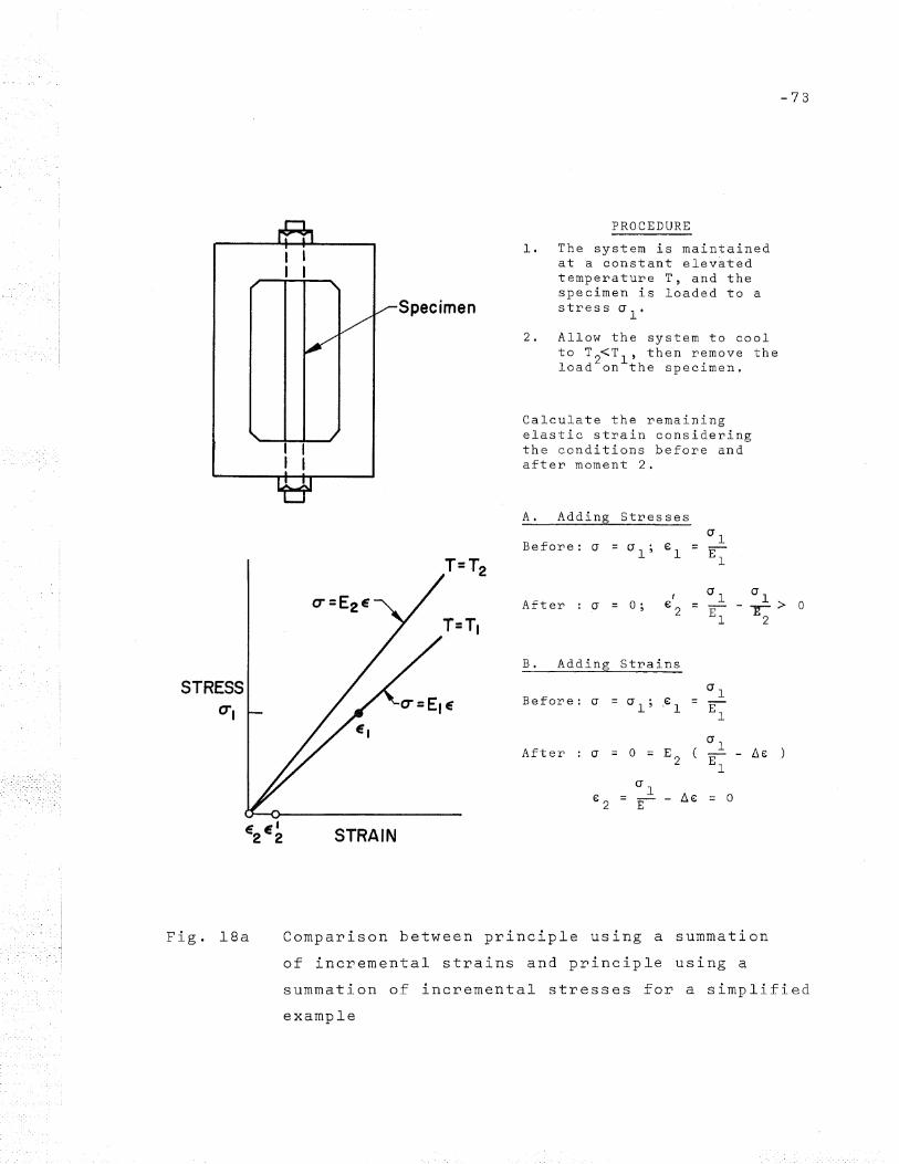
-73

PROCEDURE

Specimen

1. The system is maintainedat a constant elevatedtemperature T, and thespecimen is loaded to astress 0'1'

2. Allow the system to coolto T2<Tl~ then remove theload on the specimen.

Calculate the remainingelastic strain consideringthe conditions before andafter moment 2.

B. Adding Strains

(

a = 0; € 2

A. Adding Stresses

0"1Before: a = a 1 ; £1 = E

1

Be for e: cr = cr 1; ,€ 1

After

After 0 E2

(0"1

1:1€ )a = = E1-

€2 =°1

11€ 0E - =

STRAIN

STRESS0"'1

Fig. l8a Comparison between principle using a summation

of incremental strains and principle using a

summation of incremental stresses for a simplified

example

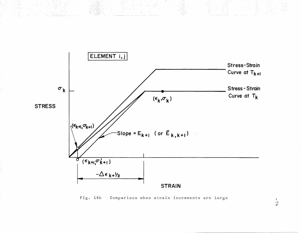
(Ek ,0-k)

STRESS

tJk

IELEMENT i,jlStress-Strain

-~~~~~~~~~~~-Curve at~+1

Stress -Strain~"'--".l-----------

Curve at Tk

Slope ::Ek +1 (or Ek,k+')

-~E k+V2

STRAIN

Fig. 18b Comparison when strain increments are large I-J+"

-75

( START

COMPUTE MATERIAL COEFFICIENTS

AT TIME t k+2

COMPUTE INCREMENTAL THERMAL STRAINS

AE!. Ii = o{. · .. r; · I.. - O{. · k .. h · LI,J, ....+1 I,J, k+2. ',J, 1't+2 I,J I I,J, K

COMPUTE STRESSES

{

Gi,j,k-+Zit£i,j,b2. IF ICi,j,k+2.Mfi,j,I<:+2.1 ~ ~iIJ,k+2

Of,j,k+'2= (SIGN Ei,j,k+2)II~i,j,k+2 IF ICi,j,k+2 t1EiJ'K+21 "7 DYi,j,k+2

COMPUTE RESULTANT STRESS

p=i AtAi,j

COMPUTE CORRECTEDSTRAINS

Gi,j,K+2.= t:i,j,k+2 -AEcorr(R)

NO

YES

COMPUTE ELASTIC STRAINS

£1~j,k+2 = Oi,j,\<.+z/Ei,j,k+2

PRINT STRESSES

Oi,j, k+2.

1CEND

Fig. 19 Short flow diagram of the subroutine for thermal

stress analysis

10

a *106

( l/oF)

5

Upper Limit of DataUsed

::==" - - .. - .. - --

® ""

Lower Limit of Data

o 400 800 1200 1600 2000

Fig. 20

TEMPERATURE (OF)

Coefficient of linear expansion. a for carbon

stressI

-.......J

m

40 000

20001600800 1200

TEMPERATURE (OF)

400

Functions U·sed

............ ............. I ............. (upper Limit of Data............. .............

" ""Lower Limit of Data -" .......... .......... ......... "'-

-........ "'-

"

---------- .........

o

10 000

300001 ---.... c::: ~ C2]=~t=-;:::::=-----

20 000

ELASTICMODULUSE (KSI)

Fig. 21 Modulus of elasticity E for carbon steels I-.J

-..J

60

2.01.5

T= 1200°F

1.0

STRAIN (0/0)

T=950°F~

0.5o

20

40

STRESS

(KSI)

Fig. 22 Schematic comparison between stress-strain curves

and the corresponding elastic-perfectly-plastic

relations with yield stress level equal to G O . 2

I-.......J

CD

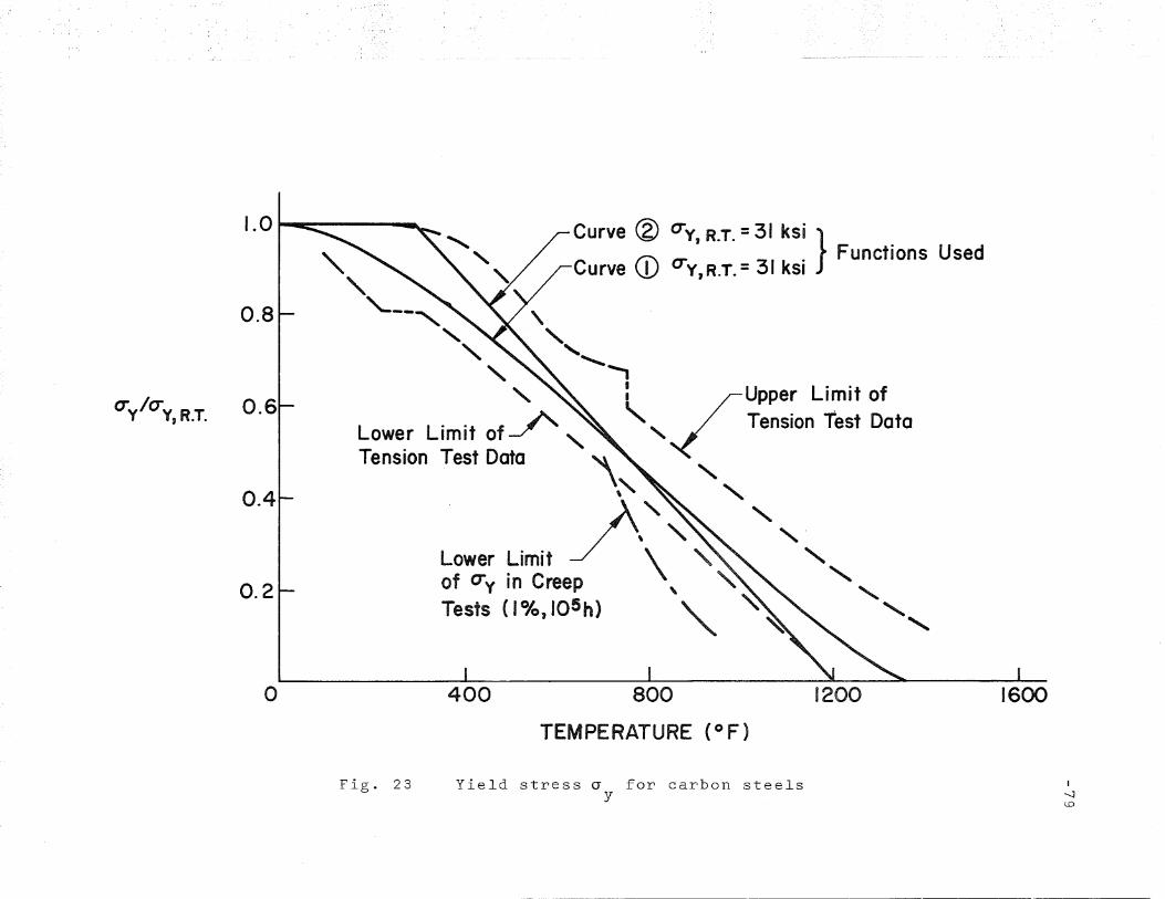
16001200

Curve ® CTy, R.T. =31 ksi

Curve CD CTY,R.T. =31 ksi } Functions Used

800

TEMPERATURE (OF)

400

"­"'---""

""" " ~ /uppe~ Limit ofLower Limit of P , " TenSion Test Data

Tension Test Data '\ '

/'~' ", " "Lower Limit \" ,

of CTy in Creep " "'-Tests (I Ok,105h) ''" ~ "

,,~ ,o

1.0 r-I ~----

0.4

0.8

0.2

CTy /CTy, R.T. O. 6

Fig. 23 Yield stress a for carbon steelsy

I

-.....J<.0

-80TEMPERATURE (OF) STRESS (KSI)

~t= 0 minI

1300

1830 !IIIIIIIIIIIIII!IIIIIIIIIIIIIIIIIIIIIIIIIIIIIIIIIIIIII111111111111111111111111111111111111111111111111111111111111111111111111111

10 min

-------...Iillllllllllllllllllllllllllllllllllllllllllill111111111111/1111111/1111111111111111111111111111111111/1111111111111/11111111111111

20min

30 min

40 min

----........-5

t ---- Q)

68

Fig. 24 Computed temperature and thermal stress behavior

during cooling of a universal-mill plate 24"x3t"

Fig. 25

-81

-20Surface

-10 AverageMid- Pfane

10

20

PL 6x ~2 (UM)

Computed residual stresses in a universal-mill

plate 6"xi"

-82

PL 20 xl (UM)

Fig. 26 Computed residual stresses in a universal-mill

plate 20"xl"

-83

-40

-30

10

_ 20 " / Surface //"Average // 7

.." ,-10' ',,- 'Mid-Plane ",' ~" "" ~, ~

O~--~~------I-~--";"'~~-----~--:""""'~'---~~~---KSI

20

PLI2x2 (UM)

Fig. 27 Computed residual stresses in a universal-mill

plate 12"x2"

-84

-40

-30 ~,/.surface

-20 Average\ .

-10'\ Mid - Plane

,,-,KSI 0 ........... ---

10 ,............... ~...

~-

20

F'ig. 28 Computed residual stresses in a universal-mill

plate 24"xsi"

-85

-40

-30 PL 24x6.. PL24x3 V2

-20 PL 24x 2

-10

KSI 0

10

20

Fig. 29 Average residual stresses across thickness for

three universal-mill plates with different

thickness

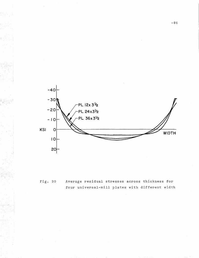
-86

-40

-30PL 12x 3

'/2

-20 PL 24x3 '/2

-10 PL 36x3'/2

KSI 0

10

20

Fig. 30 Average residual stresses across thickness for

four universal-mill plates with diffe~ent width

-87

-40

-30PL 72x3~2

-20 PL 20x I

-10 PL lOx 1/2

KSI 0

10

20

Fig. 31 Average residual stresses across thickness for

three plates with approx. same width/thickness

ratio

t=O MIN 1=2 MIN

TEMPERATURE (0 F ) 1830J

1400.# ;p "'" \\1

1505

--1--THERMAL STRESS (KSI) n 0

1·:·:·:-:-:-:·:·:·:·:·:·:·:-:;:·:·:·:·:-:·:·:-:·:-:·:·:-:.:-)

-1400

o.:.:-:-:.:.::::::::::::::::::::::::::::.:.:-:-:.:.:.:-:.:.:

t=4MIN

1295

o~: ..:.:.:.:.:.:.:~::::::::::::::::::.:.

t= 8 MIN

1110

5o 0------r-

t=16MIN

790J I

790I I

755

--U---50 0-5

t~co

70

-10

Fig. 32 Computed temperature and thermal stress behavior

during cooling of an HE 200 B shapeI00

CD

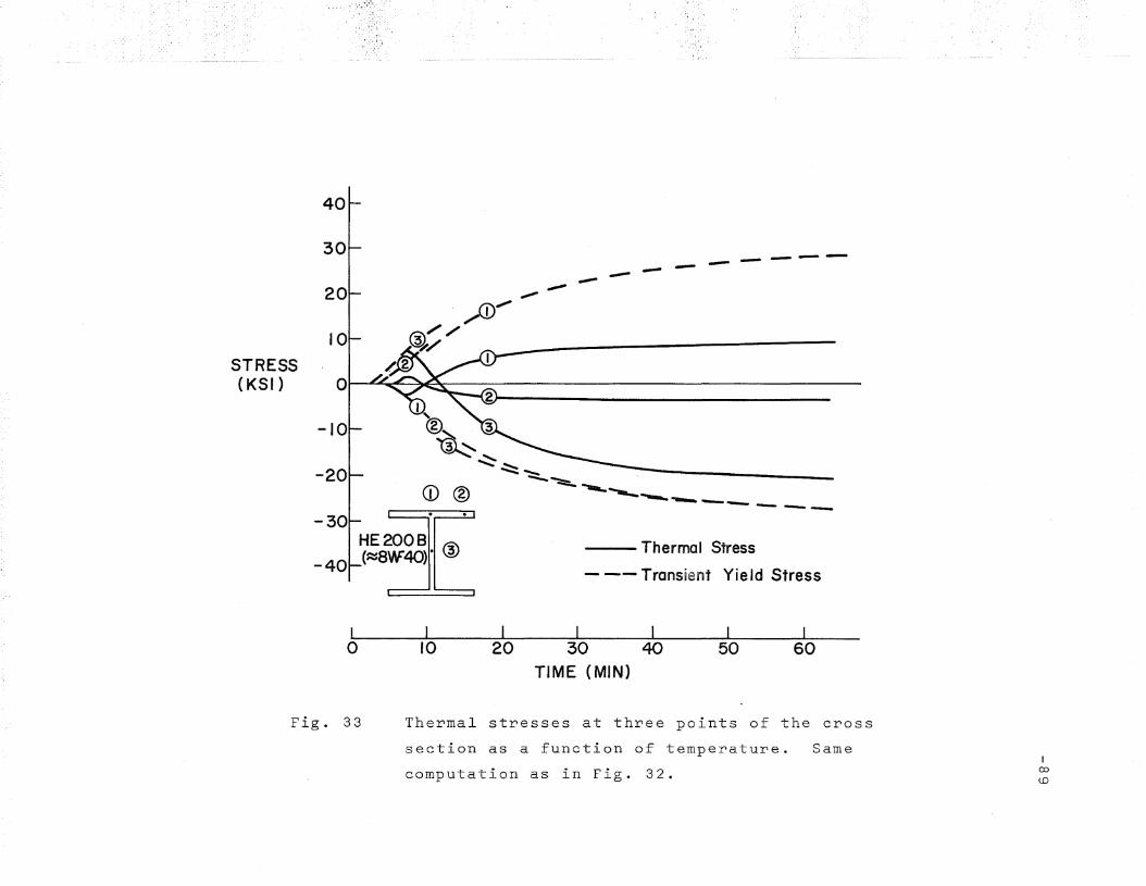
, ~ • 4 •

-------- --- ---........---,.,.""""'"

L'® ~2~

~ .....

-....;;~- ------'""::::::::.. ........--------CD®

40

30

20

10

STRESS(KSI) 0

-10

-20

-30HE200B

_40L(~8W40)1-I @ --- Thermal Stress

- -- Transient Yield Stress

L I I I I I Io 10 20 30 40 50 60

TIME (MIN)

Fig. 33 Thermal stresses at three points of the cross

section as a function of temperature. Same

computation as in Fig. 32.IcolO

-20

-10

STRESS(KSI)

10

2020

HE200B(N8YF40)--To=IB30oF

---To=2010oF

(0)

\-20

-10

ST~:I~S 0 t---Jtr------J.!-­

10

-90

20

(0

HE 200 B (l'::l8 WAD)

-a =Curve CD,Fig. 20---a=Curve ® Fig. 20

STRESS(KSI)20 10 0 ~IO -20 -30

(b)

~20

20

HE 200 8 (AlBYF40)-k=Curve CD.Flg.7- --k I:lCurve @,FIg,7

HE200B (AlBYF401

-EllCurve CD. Fig. 21

-':"-E=Curve@,Fig. 21

20

-10STRESS

(KSI·)

30

(C)

HE 200 e (Al8W40)

-cry Curvect.\Fig. 23

---cr y Curve@.Fig. 23

(d)

(a) initial temperature(b) thermal conductivity, k(0) specific heat (incl. latent heat), c(d) surface coefficien~ of heat ~ransfer~ h

(e) constant thermo-physical coefficients (k,c , and h)

(f) cgefficient of linear expansion, a(g) modulus of elasticity, E(h) yield stress, cr y

~esidual stresses.

'Fig. 34 Influence of diffe~ent assumptions on computed

Shape HE 200 B (~8WF40).

Stresses in the mid-planes of flange and web.

Fig. 35 -----Cb'-mparis-on of residual st~ess distribu-tions in

two shapes which are geometrically similar.

Stresses in the mid-planes of flange and web~

Itof-I

-92

-20

20

I

t II..

0.35 11---- ~

a"I

-20

KSI O~-----....,..

Comparison of residual stress distributions in

the HE, 200 B (';:::i8WF40) shape and a shape with

the same geometry except that wid~th is 4"

instead of 8",

..I4"I-

0.3511

0.59"

20

Fig. 36

-30

II

/I

KSI -IVf\\ "- ~/'lFree Surface Heat Transfer

---Forced II .. II

o '" ",,- ;77(Reduction at Web Surfaces)

I ~

10

20I

KSI

30 20 10 o -10 -20I I '\

~,."",.

DIP 16 /'I.. I (I

~(~6V2 x6 V4,

32Ib/ft) ,"'- "-,,

Fig. 37 Computed residual stress distribution in a

shape DIP16 when the heat transfer from the

web surface is reduced to 30-100%.ItDW

-20

--- -----10

...........

',,=''------...

....... """'"

20KSI

20 10 0 -10 -20 -30 -40

"I•I.II

II

)/",/

HE200B

--Free Heat Transfer

---Reduced Heat Transferfrom Outer Surfaces ofFlanges

---Reduced Heat Transferfrom Web and InnerSurfaces of Flanges

Fig. 38 Computed residual stress dist~ibution in a

shape HE 20q B (~8WF40) wi th different heat­

transfer assumptions

Ito

+=

Fig. 39

-95

o10

20

o

14YF426(KS I)

Computed two-dimensional variation of residual

stress in a l4WF426 shape--free heat transfer

14W-426(KSI)

-96

-10,-.-__o

....-.......--10

20

-- - --t---+--

Fig. 40 Computed two-dimensional variation of residual

stress in a 14WF426 shape--heat transfer reduced

by 50% from inner surfaces

Fig. 41

-97

14VF730( KSI)

Computed two-dimensional variation of residual

stress in a "jumbo" shape 14WF730--free heat

transfer assumed

14W-730(KS I)

20

-98

Fig. 42 Computed two-dimensional variation of residual

stress in a "jumbo" shape 14WF730--heat transfer

reduced by 50% from inner surfaces

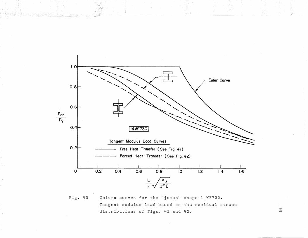
Euler Curve~-

$114\AF730 1

Tangent Modulus Load Curves

Free Heat- Transfer (See Fig. 41)

--- Forced Heat- Transfer (See Fig. 42)

"­"'" " " " " "

1.0....1------~------------....

0.4

0.2

0.6

0.8

PcrPy

o 0.2 0.4 0.6 0.8 1.0 1.2 L4 1.6

L/fiYr V-;2E

Fig. 43 Column curves for the "jumbo" shape 14WF730.

Tangent modulus load based on the residual stress

distributions of Figs. 4l and 42.

Itoto

Euler Curve

CRC BasicColumn Curve

"""~

~

Tangent Modulus LoadJ ').~Ultimate Load (CrOOkedJ "Column with uo=O.OOIL) ~

~~

tp

1.01 •

0.8

0.6

0.4

0.2

PerPy

14YF730 Weak Axis, Residual Stresses According to Fig. 41

o 0.2 0.4 0.6 0.8

..ho~ IJ"yr 7T2E

1.0 1.2 1.4 1.6

Fig. 44 Comparison between tangent modulus load. and

ultimate strength of the 14WF730 shape with

residual stresses accordlng to Fig. 41.

If---Jao

20

15

COMPUTEDcrRC 10

(KS I)

5

90

0 0

~ 0 869 8

00

0 00

o

o

o

o

o00

o 0.2

o

0.4bitd/w

0.6 0.8 1.0

Fig. 45 Average residual stress at flange tips of H­

shapes, plotted against a geometrical parameter

bitd/w

Il---Jof---J

1.00.80.60.40.2

5

o

20

15Medium

IShapes

I

COMPUTEDuRC lOr- I Small

(KS I) Sh-apes

bitd/w

Fig. 46 Schematic diagram showing the principal

influence of shape geometry upon residual

stresses at flange tips of H-shapes

I.......,

or'0

-103

-20

-10~

" ;I'

KSI 0 .......

10

---- Experimental Results (Ref. 22)

- --Computed Curve

-20

KSI O~---=~=-----------=------::a:~--

-10 /

10

--- Experimental Results (Ref. 22)

---Computed Curve

-20

-10

KSI 0r-~~=-:;;:::E~~=::=;~~~""""-=---

10

• • Experimental Results (Ref. 22)

PL 20llx III (UM) --0----0-- Experimental Results (Ref. 23)

--- Computed Curve

Fig. 47 Comparison between computed residual stresses

and experimentally measured residual st~esses

for universal-mill plates

-10

KSI O~, ~

\\

fOr- ,'-....../ /'-----/

-~- Experimental Results (Ref. 24)

-- - Computed Curves

20

20KSI

1-0-' 0 ~ 10 ~2-0· -30

/,;'"",

.,."."

~

IPE 200(~811X411J

15 Ib/ft)

Fig. 4.8 Residual st~esses in·a European I-beam IPE200

IHo+:"

-105

-20

~ ~ Experimental Results(Ref. 7)

--- Computed Curves

KSI20 10 0 -10 -20

10

20

-10

KSI Ot----~------JC---

6M15.5

"20

10

KSI 0 n/ ~

-10 / ~,-20

Fig. 49 Residual stresses in a 6M15.5 shape

-106

-10-0--0- Experimental Results

KSI 0(Ref. 25)

- --Computed Curves

20

30 KSI

30 20 10 0 -10I 1

....................

"'1

IIII

12W31 IIII

I)

",-/'

"""..,.".................--........

I I t

Fig. 5 a Residual stresses in a 12WF3l shape

-107

--Experimental Results (Ref. 7)

- -- Experimental Results; MemberCooled Separately on CoolingBed (Ref. 7)

--- Computed Curve

30 20 10 0 -10 -20 -30 -40

14'N=43

30

20

KS I o~-------w.--

-10

-20

Fig. 51 Residual stresses in a 14WF43 shape

-108

-20

-0-0-- Experimental Results (Ref. 25)

- - - Computed Curves

-10

20

30 KSI

30 20 10 0 -10 -20 -30 -40I 1

...................

'1II

III

16W50 IIIIII

_..J

--- ---...........I c.:-- ---

KSI 01'+'--------1'1--

Fig. 52 Residual stresses in a 16WF50 shape

-109 .

-10

--0-0- Experimental Results (Ret 25)

- - - Computed Curves

KSI30, 20 10 0 -10 -20 -30 -40

I

I

10

r

o......-------~

30

20

27WI02

KSI

Fig. 53 Residual stresses in a 27WFI02 shape

-110

-30

-20 '

-10

KS I Ot--~"""'--~'--"I---

10

20

14W426

20

- 30

~ Experimental Results (Ref. 7)

-- Computed Curves

Free Heat Transfer

Reduced Heat Transfer

KSI20 10 0 -10 -20 -30

Reduced HeatTransfer

Fig. 54 Residual stresses in a 14WF426 shape

I4'IF 730(KS I)

-Ill

Fig. 55 Residual stresses in a 14WF730 shape

337.3

REFERENCES

1. G. A. Alpsten and L. TallRESIDUAL ·STRESSES IN HEAVY WELDED SHAPES,Fritz Laboratory Report No. 337.12,In Preparation.

2. G. AlpstenEGENSPANNINGAR I VARMVALSADE STALPROFILER(RESIDUAL STRESSES IN HOT-ROLLED STEEL .PROFILES),Tekn. Lie. Dissertation, Institution ofStructural Engineering and Bridge Building,The Royal Institute of Technology,Stockholm, 1967.

3. M. RosDIE BREITFLANSCHIGEN DIFFERDINGER-GREY-TRAGER(THE WIDE-FLANGE SHAPES, TYPE DIFFERDINGER­GREY), Bericht 52, Eidgen. Mat.-Prlif.-Anst. ,.Techn. Hochsch.~ Zurich, 1930.

4. J. MatharERMITTLUNG VON EIGENSPANNUNGEN DURCH MESSUNG

·VON BOHRLOCH-VERfORMUNGEN (DETERMINATION OFRESIDUAL STRESSES BY MEASURING THE DEFORMATIO~

AROUND DRILLED HOLES), Archiv f.d. EisenhlittenwesenVol. 6, 1933, pp. 277-281.

5. O. GraveDISCUSSION TO REF. 4

6. DornenSCHRUMPFUNGEN AN GESCHWEISSrEN STAHLB~UTEN,

Stahlbau, Vol. 6, 1933, pp. 22-24.

7. Y. FujitaTHE MAGNITUDE AND DISTRIBUTION OF RESIDUALSTRESSES, Fritz Laboratory Report No. 2.20A.20,May, 1955.

8. A. W. HuberTHE INFLUENCE OF RESIDUAL STRESS ON THEINSTABILITY OF COLUMNS, Ph.D. Dissertation,Lehigh University, 1956

9. L. S. Beedle and L. TallBASIC COLUMN STRENGTH, Proe. ASCE, Vol. 86,1960, pp. 139-173.

-112

337.3 -113

10. B. A. Boley and J. H. WeinerTHEORY OF THERMAL STRESS, John Wiley &Sons, Inc., 1960.

11. D. W. Peaceman and H. H. RachfordTHE NUMERICAL SOLUTION OF PARABOLIC ANDELLIPTIC DIFFERENTIAL EQUATIONS, J. Soc.Indust. Appl. Math., Vol. 3,1955, pp. 28-41.

12. G. Birkhoff and R. S. VargaIMPLICIT ALTERNATING DIRECTION METHODS,Trans. Amer. Math. Soc., Vol. 92, 1959, pp. 13-24.

13. G. A. AlpstenTHE PREDICTION OF COOLING BEHAVIOR OF HOT-ROLLEDST~EL MEMBERS, Fritz Laboratory Report No. 337.13,In Preparation

14. N. R. Eyres, D. R. Hartree, J. Ingham, R. Jackson,R. J. Sarjant, and J. B. Wagstaff

THE CALCULATION OF VARIABLE HEAT FLOW INSOLIDS, Phil. Trans., Royal Society ofLondon, Vol. 240, 1946, Serf A, pp. 1-57.

15. G. M. DusinberreNUMERICAL METHODS FOR TRANSIENT HEAT FL'OW,Trans., Am. Soc. Mechanical Engrs., Vol. 67,1945, pp. 703-712.

16. K. OdeenBERAKNING AV ICKE-STATIONAR, TVA-DIMENSIONELLVARMELEDNING I BRAND-UTSATTA BETONGKONSTRUKTIONER(CALCULA.TION OF NON-STATIONARY, TWO-DIMENSIONALHEAT FLOW IN CONCRETE STRUCTURES SUBJECTED TOFIRE) Vag-oeh vattenbyggaren, Stockholm, No. 11,1964, pp. 463-466.

17. L. TallRESIDUAL STRESSES IN WELDED PLATES -- ATHEORETICAL ST~DY, The' Welding Journal,Vol. 43, Jan. 1964, pp. 10-8 - 23-s.

18. D. V. Lindh and J. L. TocherHEAT GENERATION AND RESIDUAL STRESS DEVELOPMENTIN RESISTANCE SPOT WELDING, The Welding Journal,Vol. 46, Aug. 1967, pp. 351-s - 360-s.

19. F. R. EstuarWELDING RESIDUAL STRESSES AND THE STRENGTHOF HEAVY COLUMN SHAPES, Ph.D. Dissertation,Lehigh University, Aug., 1965. (UniversityMicrofilm Inc., Ann Arbor, Michigan).

337.3 -114

20. J. GlenAN EXPERIMENTAL STUDY OF THE STRENGTH AND'DUCTILITY OF STEEL AT ELEVATED TEMPERATURES,Symp. on Strength and Ductility of Metals, 1952,pp. 184-221.

2 1 • B. G. J a h n st 0 n ( Ed. )GUIDE TO DESIGN CRITERIA FOR METAL COMPRESSIONMEMBERS, 2nd Edition, 1966, Column Resea~ch Council.

22. N. R. NagarajaRao and L. TallRESIDUAL STRESSES IN WELDED PLATES, WeldingJournal, Vol. 40, Oct., 1961, pp. 468-s - 480-s.

-23. M. Lohrmann, N. R. NagarajaRao and L. TallRESIDUAL STRESSES IN AUTOMATICALLYWELDED PLATES, Fritz Laboratory Report,In Preparation.

24. E. Mas and C. MassonnetBELGIUM'S, PART IN THE EXPERIMENTALRESEARCH ON THE BUCKLING OF AXIALLYLOADED MILD-STEEL MEMBERS CONDUCTEDBY THE "CONVENTION EUROPEENNE DE LACO~STRUCTION METALLIQUE", Acier-Stahl-Steel,No.9, Sept., 1966, pp. 385-392.

25. A. FranklinPRIVATE COMMUNICATIONS, 1967.

26. J. Brozzetti, G. A. A1psten, and L. TallRESIDUAL STRESSES IN A HEAVYROLLED SHAPE 14WF730,Fritz Laboratory Report No. 337.10,In Preparation.

27. G. A. Alpsten and L. TallCOLUMN STRENGTH OF HEAVY SHAPES - A PROGRESS REPORT,Fritz Laboratory Report No. 337.16,In Preparation.