THERMODYNAMIC TREE: THE SPACE OF ADMISSIBLE PATHS

ALEXANDER N. GORBAN∗

Abstract. Is a spontaneous transition from a state x to a state y allowed by thermodynamics?Such a question arises often in chemical thermodynamics and kinetics. We ask the more formalquestion: is there a continuous path between these states, along which the conservation laws hold, theconcentrations remain non-negative and the relevant thermodynamic potential G (Gibbs energy, forexample) monotonically decreases? The obvious necessary condition, G(x) ≥ G(y), is not sufficient,and we construct the necessary and sufficient conditions. For example, it is impossible to overstepthe equilibrium in 1-dimensional (1D) systems (with n components and n−1 conservation laws). Thesystem cannot come from a state x to a state y if they are on the opposite sides of the equilibrium evenif G(x) > G(y). We find the general multidimensional analogue of this 1D rule and constructivelysolve the problem of the thermodynamically admissible transitions.

We study dynamical systems, which are given in a positively invariant convex polyhedron andhave a convex Lyapunov function G. An admissible path is a continuous curve along which G doesnot increase. For x, y ∈ D, x < y (x precedes y) if there exists an admissible path from x to y andx ∼ y if x < y and y < x. The tree of G in D is a quotient space D/ ∼. We provide an algorithmfor the construction of this tree. In this algorithm, the restriction of G onto the 1-skeleton of D(the union of edges) is used. The problem of existence of admissible paths between states is solvedconstructively. The regions attainable by the admissible paths are described.

Key words. Lyapunov function, convex polyhedron, attainability, tree of function, entropy, freeenergy

AMS subject classifications. 37A60, 52A41, 80A30, 90C25

1. Introduction.

1.1. Ideas and a simple example. “Applied dynamical systems” are modelsof real systems. We never know such systems in full detail. The available informationabout the system is incomplete and there are uncertainties of various types: errors inthe model structure, errors in coefficients, in the state observation and many others.Nevertheless, there is an order in this world of errors: some information is morereliable, we trust in some structures more and even respect them as laws. Some otherdata are less reliable. There is an hierarchy of reliability, our knowledge and beliefs(described, for example by R. Peierls [44] for model making in physics). Extractingas many consequences from the more reliable data either without or before use of theless reliable information is a task which arises naturally.

In our paper, we study the systems of chemical kinetics and thermodynamics. Forthem, we can rank the information in the following way. First of all, the list of reagentsand conservation laws should be known. Let the reagents be A1, A2, . . . , An. The non-negative real variable Ni ≥ 0, the amount of Ai in the mixture, is defined for eachreagent, and N is the vector of composition with coordinates Ni. The conservationlaws are presented by the linear balance equations:

bi(N) =n∑

j=1

ajiNj = const (i = 1, . . . ,m) . (1.1)

We assume that the linear functions bi(N) (i = 1, . . . ,m) are linearly independent.The list of the components together with the balance conditions (1.1) is the first

part of the information about the kinetic model. This determines the space of states,

∗Department of Mathematics, University of Leicester, UK (ag153@le.ac.uk).

1

2 A. N. GORBAN

the polyhedronD defined by the balance equations (1.1) and the positivity inequalitiesNi ≥ 0. This is the background of kinetic models and any further development is lessreliable.

The polyhedron D is assumed to be bounded. This means that there exist suchcoefficients λi that the linear combination

∑i λibi(N) has strictly positive coefficients:∑

i λiaji > 0 for all j = 1, . . . , n.

The thermodynamic functions provide us with the second level of informationabout the kinetics. Thermodynamic potentials, such as the entropy, energy and freeenergy are known much better than the reaction rates and, at the same time, theygive us some information about the dynamics. For example, the entropy increases inisolated systems. The Gibbs free energy decreases in closed isothermal systems underconstant pressure, and the Helmholtz free energy decreases under constant volumeand temperature. Of course, knowledge of the Lyapunov functions gives us someinequalities for vector fields of the systems’ velocity but the values of these vectorfields remain unknown. If there are some external fluxes of energy or non-equilibriumsubstances then the thermodynamic potentials are not Lyapunov functions and thesystems do not relax to the thermodynamic equilibrium. Nevertheless, the inequalityof positivity of the entropy production persists and this gives us useful informationeven about the open systems. Some examples are given in [22].

The next, third part of the information about kinetics is the reaction mechanism.It is presented in the form of the stoichiometric equations of the elementary reactions:

∑

i

αρiAi →∑

i

βρiAi , (1.2)

where ρ = 1, . . . ,m is the reaction number and the stoichiometric coefficients αρi, βρi

(i = 1, . . . , n) are nonnegative integers.A stoichiometric vector γρ of the reaction (1.2) is a n-dimensional vector with

coordinates

γρi = βρi − αρi , (1.3)

that is, ‘gain minus loss’ in the ρth elementary reaction.The concentration of Ai is an intensive variable ci = Ni/V , where V > 0 is the

volume. The vector c = N/V with coordinates ci is the vector of concentrations.A non-negative intensive quantity, rρ, the reaction rate, corresponds to each re-

action (1.2). The kinetic equations in the absence of external fluxes are

dN

dt= V

∑

ρ

rργρ . (1.4)

If the volume is not constant then equations for concentrations include V and havedifferent form.

For perfect systems and not so fast reactions the reaction rates are functions ofconcentrations and temperature given by the mass action law and by the generalized

Arrhenius equation. The mass action law is

rρ(c, T ) = kρ(T )∏

i

cαρi

i , (1.5)

where kρ(T ) is the reaction rate constant.

THERMODYNAMIC TREE 3

The generalized Arrhenius equation is

kρ(T ) = Aρ exp

(Saρ

R

)exp

(−Eaρ

RT

), (1.6)

where R = 8.314 472 JK mol is the universal, or ideal gas constant, Eaρ is the activation

energy, Saρ is the activation entropy (i.e. Eaρ − TSaρ is the activation free energy),and Aρ is the constant pre-exponential factor. A special relation between the kineticconstants is given by the principle of detailed balance: For each value of temperature Tthere exists a positive equilibrium point where each reaction (1.2) is equilibrated withits reverse reaction. This principle was introduced for collisions by Boltzmann in 1872[6]. Einstein in 1916 used this principle in the background for his quantum theoryof emission and absorption of radiation [11]. Wegscheider introduced the principle ofdetailed balance for chemical kinetics in 1901 [54]. Later, it was used by Onsager inhis famous work [43]. For a recent review see [24].

At the third level of reliability of information we select the list of componentsand the balance conditions, find the thermodynamic potential, guess the reactionmechanism, accept the principle of detailed balance and believe that we know thekinetic law of elementary reactions and the character of dependencies kρ(T ). However,we still do not know the reaction rate constants.

Finally, at the fourth level of available information, we find the reaction rateconstants and can analyze and solve the kinetic equations (1.4) or their extendedversion with the inclusion of external fluxes.

Of course, this ranking of the available information is conventional, to a cer-tain degree. For example, some reaction rate constants may be known even betterthan the list of intermediate reagents. Nevertheless, this hierarchy of the informationavailability, list of components – thermodynamic functions – reaction mechanism –reaction rate constants, reflects the real process of modelling and the stairs of availableinformation about a reaction kinetic system.

It seems very attractive to study the consequences of the information of eachlevel separately. These consequences can be also organized ‘stairwise’. We have thehierarchy of questions: how to find the consequences for the dynamics (i) from the listof components, (ii) from this list of components plus the thermodynamic functions ofthe mixture, and (iii) from the additional information about the reaction mechanism.

The answer to the first question is the description of the balance polyhedron D.The balance equations (1.1) together with the positivity conditions Ni ≥ 0 shouldbe supplemented by the description of all the faces. For each face, some Ni = 0 andwe have to specify which Ni have zero value. The list of the corresponding indicesi, for which Ni = 0 on the face, I = {i1, . . . , ik}, fully characterizes the face. Thisproblem of double description of the convex polyhedra [42, 9, 15] is well know in linearprogramming.

The list of vertices and edges with the corresponding indices is necessary for thethermodynamic analysis. This is the 1-skeleton of D. Algorithms for the construc-tion of the 1-skeletons of balance polyhedra as functions of the balance values weredescribed in detail in 1980 [20]. The related problem of double description for convexcones is very important for the pathway analysis in systems biology [46, 16].

In this work, we use the 1-skeleton of D, but the main focus is on the second step,i.e. on the consequences of the given thermodynamic potentials. For closed systemsunder classical conditions, these potentials are the Lyapunov functions for the kineticequations. For example, for perfect systems we assume the mass action law. If the

4 A. N. GORBAN

A1

A2 A3

c*

c1=c3=1/2

G(c)=g0

G(c)>g0

G(c)<g0

c1=c2=1/2

c1≈0.773

b)

c

c1

A1

A2 A3

a)

c) G

G(c*)

g0

gmax

c*

A1 A2 A3

A1

A2 A3

c*

d)

c

c'

c*'

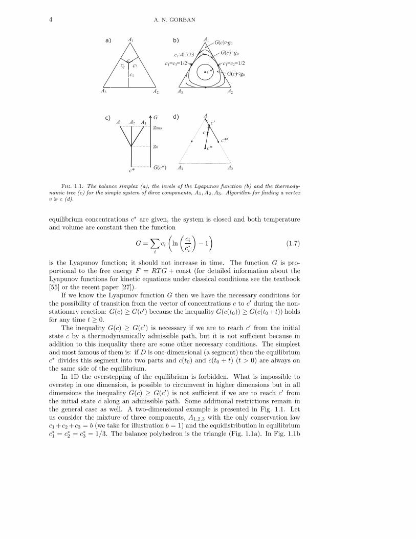
Fig. 1.1. The balance simplex (a), the levels of the Lyapunov function (b) and the thermody-namic tree (c) for the simple system of three components, A1, A2, A3. Algorithm for finding a vertexv < c (d).

equilibrium concentrations c∗ are given, the system is closed and both temperatureand volume are constant then the function

G =∑

i

ci

(ln

(cic∗i

)− 1

)(1.7)

is the Lyapunov function; it should not increase in time. The function G is pro-portional to the free energy F = RTG + const (for detailed information about theLyapunov functions for kinetic equations under classical conditions see the textbook[55] or the recent paper [27]).

If we know the Lyapunov function G then we have the necessary conditions forthe possibility of transition from the vector of concentrations c to c′ during the non-stationary reaction: G(c) ≥ G(c′) because the inequality G(c(t0)) ≥ G(c(t0 +t)) holdsfor any time t ≥ 0.

The inequality G(c) ≥ G(c′) is necessary if we are to reach c′ from the initialstate c by a thermodynamically admissible path, but it is not sufficient because inaddition to this inequality there are some other necessary conditions. The simplestand most famous of them is: if D is one-dimensional (a segment) then the equilibriumc∗ divides this segment into two parts and c(t0) and c(t0 + t) (t > 0) are always onthe same side of the equilibrium.

In 1D the overstepping of the equilibrium is forbidden. What is impossible tooverstep in one dimension, is possible to circumvent in higher dimensions but in alldimensions the inequality G(c) ≥ G(c′) is not sufficient if we are to reach c′ fromthe initial state c along an admissible path. Some additional restrictions remain inthe general case as well. A two-dimensional example is presented in Fig. 1.1. Letus consider the mixture of three components, A1,2,3 with the only conservation lawc1 +c2 +c3 = b (we take for illustration b = 1) and the equidistribution in equilibriumc∗1 = c∗2 = c∗3 = 1/3. The balance polyhedron is the triangle (Fig. 1.1a). In Fig. 1.1b

THERMODYNAMIC TREE 5

the level sets of

G =

3∑

i=1

ci(ln(3ci) − 1)

are presented. This function achieves its minimum at equilibrium, G(c∗) = −1. Onthe edges, the function G achieves its conditional minimum, g0, in the middles, andg0 = ln(3/2)− 1. G reaches its maximal value, gmax = ln 3 − 1, at the vertices.

If G(c∗) < g ≤ g0 then the level set G(c) = g is connected. If g0 < g ≤ gmax thenthe corresponding level set G(c) = g consists of three components (Fig. 1.1b). Thecritical value is g = g0. The critical level G(c) = g0 consists of three arcs. Each arcconnects two middles of the edges and divides D in two sets. One of them is convexand includes two vertices, the other includes the remaining vertex.

A thermodynamically admissible path is a continuous curve along which G doesnot increase. Therefore, such a path cannot intersect these arcs ‘from inside’, i.e.from values G(c) ≤ g0 to bigger values, G(c) > g0. For example, if an admissible pathstarts from the state with 100% of A2, then it cannot intersect the arc that separatesthe vertex with 100% A1 from two other vertices. Therefore, any vertex cannot bereached from another one and if we start from 100% of A2 then the reaction cannotovercome the threshold ∼77.3% of A1, that is the maximum of c1 on the correspondingarc (Fig. 1.1b). This is an example of the 2D analogue of the 1D prohibition ofoverstepping of equilibrium.

For x, y ∈ D, x < y (x precedes y) if there exists an admissible path from x to yand x ∼ y if x < y and y < x. The tree of G in D is a quotient space T = D/ ∼.For the natural projection D → D/ ∼ we use the notation π. The tree D/ ∼ is a1D continuum. We have to distinguish these connected acyclic graphs which have thesame graphical representation but are discrete objects.

If x ∼ y then G(x) = G(y). Therefore, we can define the function G on thetree: G(π(c)) = G(c). It is convenient to draw this tree on the plane with the verticalcoordinateG(x) (Fig. 1.1c). Equilibrium c∗ corresponds to a root of this tree, π(c∗). IfG(c∗) < g ≤ g0 then the level set G(c) = g corresponds to one point on the tree. Thelevel G(c) = g0 corresponds to the branching point, and each connected componentof the level sets G(c) = g with g0 < g ≤ gmax corresponds to a separate point on thetree. The terminal leaves of the tree correspond to the vertices of D.

Let x, y ∈ T and x 6= y. The point z ∈ T is between x and y if T \ {z} is notconnected, T \ {z} = T1 ∪ T2, T1 and T2 are connected, x ∈ T1 and y ∈ T2. In otherwords, z is a cut point that separates x from y.

The open segment (x, y) consists of all points that are between x and y. Theclosed segment [x, y] = (x, y) ∪ {x, y}. These segments are homeomorphic to openand closed segments on the real line.

A continuous curve ϕ : [0, 1] → D is an admissible path if and only if its imageπ ◦ ϕ : [0, 1] → T is a path that goes monotonically down in the coordinate g.For each point x ∈ T , the region attainable by the admissible paths (the attainable

region) is just a segment [x, π(c∗)]. On such a segment each point is unambiguouslycharacterized by the value of G. Therefore, if for c ∈ D we know the value G(c) anda vertex v < c, then we can unambiguously describe the image of c on the tree: π(c)is the point on the segment [π(v), π(c∗)] with the given value of G, g = G(c).

We can find a vertex v < c by the following algorithm:

• If c = c∗ then any vertex v of D precedes c, v < c.

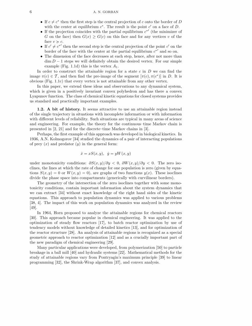
6 A. N. GORBAN

• If c 6= c∗ then the first step is the central projection of c onto the border of Dwith the center at equilibrium c∗. The result is the point c′ on a face of D.

• If the projection coincides with the partial equilibrium c∗′ (the minimizer ofG on the face) then G(x) ≥ G(c) on this face and for any vertices v of theface v < c.

• If c′ 6= c∗′ then the second step is the central projection of the point c′ on theborder of the face with the center at the partial equilibrium c∗′ and so on.

• The dimension of the face decreases at each step, hence, after not more thandimD − 1 steps we will definitely obtain the desired vertex. For our simpleexample (Fig. 1.1d) this is the vertex A1.

In order to construct the attainable region for a state c in D we can find theimage π(c) ∈ T , and then find the pre-image of the segment [π(c), π(c∗)] in D. It isobvious (Fig. 1.1c) that every vertex is not attainable from any other vertex.

In this paper, we extend these ideas and observations to any dynamical system,which is given in a positively invariant convex polyhedron and has there a convexLyapunov function. The class of chemical kinetic equations for closed systems providesus standard and practically important examples.

1.2. A bit of history. It seems attractive to use an attainable region insteadof the single trajectory in situations with incomplete information or with informationwith different levels of reliability. Such situations are typical in many areas of scienceand engineering. For example, the theory for the continuous–time Markov chain ispresented in [2, 21] and for the discrete–time Markov chains in [3].

Perhaps, the first example of this approach was developed in biological kinetics. In1936, A.N. Kolmogorov [34] studied the dynamics of a pair of interacting populationsof prey (x) and predator (y) in the general form:

x = xS(x, y), y = yW (x, y)

under monotonicity conditions: ∂S(x, y)/∂y < 0, ∂W (x, y)/∂y < 0. The zero iso-clines, the lines at which the rate of change for one population is zero (given by equa-tions S(x, y) = 0 or W (x, y) = 0), are graphs of two functions y(x). These isoclinesdivide the phase space into compartments (generically with curvilinear borders).

The geometry of the intersection of the zero isoclines together with some mono-tonicity conditions, contain important information about the system dynamics thatwe can extract [34] without exact knowledge of the right hand sides of the kineticequations. This approach to population dynamics was applied to various problems[38, 4]. The impact of this work on population dynamics was analyzed in the review[49].

In 1964, Horn proposed to analyze the attainable regions for chemical reactors[30]. This approach became popular in chemical engineering. It was applied to theoptimization of steady flow reactors [17], to batch reactor optimization by use oftendency models without knowledge of detailed kinetics [13], and for optimization ofthe reactor structure [28]. An analysis of attainable regions is recognized as a specialgeometric approach to reactor optimization [12] and as a crucially important part ofthe new paradigm of chemical engineering [29].

Many particular applications were developed, from polymerization [50] to particlebreakage in a ball mill [40] and hydraulic systems [22]. Mathematical methods for thestudy of attainable regions vary from Pontryagin’s maximum principle [39] to linearprogramming [32], the Shrink-Wrap algorithm [37], and convex analysis.

THERMODYNAMIC TREE 7

The connection between attainable regions, thermodynamics and stoichiometricreaction mechanisms was studied in the 1970s. In 1979 it was demonstrated how toutilize the knowledge about partial equilibria of elementary processes to construct theattainable regions [18]. It is possible to use the attainable regions for the discrimi-nation of reaction mechanisms [23] because these regions significantly depend on themechanism.

Thermodynamic data are more robust than the reaction mechanism and the re-action rates are known with lower accuracy than the stoichiometry of elementaryreactions. Hence, there are two types of attainable regions. The first is the ther-modynamic one, which use the linear restrictions and the thermodynamic functions[19]. The second is generated by thermodynamics and stoichiometric equations ofelementary steps (but without reaction rates) [18, 25]. R. Shinnar and other authors[48] rediscovered this approach. There was even an open discussion about priority [5].This geometric approach is applied now to various chemical and industrial processes.

Some particular classes of kinetic systems have rich families of the Lyapunovfunctions. Krambeck [35] studied attainable regions for linear systems and the l1Lyapunov norm instead of the entropy. Already simple examples demonstrate thatthe sets of distributions which are accessible from a given initial distribution by linearkinetic systems (Markov processes) with a given equilibrium are, in general, non-

convex polytopes [18, 21, 57]. The non-convexity makes the analysis of attainabilityfor continuous time Markov processes more difficult and interesting. This geometricapproach to attainability was developed for all the thermodynamic potentials andfor open systems as well [20]. Partial results for chemical kinetics and some otherengineering systems are summarized in [55, 22].

The tree of the level sets for differentiable functions was studied in the middleof the 20 century by Adelson-Velskii and Kronrod [1, 36] and Reeb [45]. Sometimesthese trees are called the Reeb trees [14] but from the historical point of view it maybe better to call them the Adelson-Velskii – Kronrod – Reeb (or AKR) trees. Thisidea has application in differential topology (the Morse theory [41]), in topologicalshape analysis and visualization [14, 33] and in data analysis [51].

Some time ago this tree was recognized as an adequate tool for representationof the attainable regions in chemical thermodynamics [19, 20]. It was applied foranalysis of various real systems [31, 56]. Nevertheless, some of the mathematicalbackgrounds of this approach were delayed in development and publications. Now,the thermodynamically attainable regions are in extensive use in chemical engineeringand beyond [12, 13, 17, 22, 28, 29, 30, 31, 32, 35, 37, 39, 40, 47, 48, 50, 56]. In thispaper we aim to provide the complete mathematical background for the analysis ofthe thermodynamically attainable regions.

1.3. The Structure of the Paper. Our results are applicable to any familyof dynamical systems that obey a continuous strictly convex Lyapunov function in apositively invariant convex polyhedron.

In Sec. 2 we present several auxiliary propositions from convex geometry. Weconstructively describe the result of the cutting of a convex polyhedron D by a convexset U : we demonstrate, how it is possible to describe the connected components ofD \ U by the analysis of the 1D continuum D1 \ U , where D1 is the 1-skeleton of D.

In Sec. 3, we construct the tree of level sets of a strictly convex function G in theconvex polyhedron D and study the properties of this tree. The main result of thissection is the algorithm for construction of this tree (Sec. 3.3). These constructionsare applied to several examples from chemical kinetics in Sec. 4.

8 A. N. GORBAN

2. Cutting of a polyhedron D by a convex set U .

2.1. Connected components of D \ U and of D1 \ U . Here and below, D isa convex polyhedron in R

n. Aff(D) is the minimal linear manifold that includes D.d = dimAff(D) = dimD is the dimension of D. ri(D) is the interior of D in Aff(D);r∂(D) is the border of D in Aff(D).

Let, for P,Q ⊂ Rn. The Minkowski sum is P +Q = {x+ y |x ∈ P, y ∈ Q}. The

convex hull (conv) and the conic hull (cone) of a set V ⊂ Rn are:

conv(V ) =

{q∑

i=1

λivi

∣∣∣∣∣ q > 0, v1, . . . , vq ∈ V, λ1, . . . λq > 0,

q∑

i=1

λi = 1

};

cone(V ) =

{q∑

i=1

λivi

∣∣∣∣∣ q ≥ 0, v1, . . . , vq ∈ V, λ1, . . . λq > 0,

}.

For a set D ⊂ Rn the following two statements are equivalent (the Minkowski–Weyl

theorem):1. For some real (finite) matrix A and real vector b, D = {x ∈ R

n |Ax ≤ b} ;2. There are finite sets of vectors {v1, . . . , vq} ⊂ R

n and {r1, . . . rp} ⊂ Rn such

that

D = conv{v1, . . . vq} + cone{r1, . . . , rp} (2.1)

.Every polyhedron has two representations, of type (1) and (2), known as (halfspace)H-representation and (vertex) V -representation, respectively. We systematically useboth these representations. Most of the polyhedra in our paper are bounded, therefore,for them only the convex envelope of vertices is used in the V -representation (2.1).

The k-skeleton of D, Dk, is the union of the closed k-dimensional faces of D:

D0 ⊂ D1 ⊂ . . . ⊂ Dd = D .

D0 consists of vertices of D and D1 is a one-dimensional continuum embedded in Rn.

We use the notation D1 for the graph whose vertices correspond to the vertices of Dand edges correspond to the edges of D, and call this graph the graph of the 1-skeleton

of D.The closed segment in R

n with ends x, y is [x, y] = {λx+ (1 − λ)y |λ ∈ [0, 1]}.Let U be a convex subset of R

n (it may be a non-closed set). We use U0 for theset of vertices of D that belong to U , U0 = U ∩D0, and U1 for the set of the edges ofD that have non-empty intersection with U . By default, we consider the closed facesof D, hence, the intersection of an edge with U either includes some internal pointsof the edge or consists from one of its ends. We use the same notation U1 for the setof the corresponding edges of D1.

A set W ⊂ P ⊂ Rn is a path – connected component of P if it is its maximal

path – connected subset. In this section, we aim to describe the path – connectedcomponents of D \ U . In particular, we prove that these components include the

same sets of vertices as the connected components of the graph D1 \U . This graph is

produced from D1 by deletion of all the vertices that belong to U0 and all the edgesthat belong to U1.

THERMODYNAMIC TREE 9

The closed segment in Rn with ends x, y is [x, y] = {λx+ (1 − λ)y |λ ∈ [0, 1]}.

Lemma 2.1. Let x ∈ D \ U . Then there exists such a vertex v ∈ D0 that the

closed segment [v, x] does not intersect U : [v, x] ⊂ D \ U .

Proof. Let us assume the contrary: for every vertex v ∈ D0 there exists suchλv ∈ (0, 1] that x + λv(v − x) ∈ U . The convex polyhedron D is the convex hullof its vertices. Therefore, x =

∑v∈D0

κvv for some numbers κv ≥ 0, v ∈ DO,∑v∈D0

κv = 1.Let

δv =κv

λv

∑v′∈D0

κv′

λv′

.

It is easy to check that∑

v∈D0δv = 1 and

x =∑

v∈D0

δv(x+ λv(v − x)) . (2.2)

According to (2.2), x belongs to the convex hull of the finite set {x+ λv(v − x) | v ∈D0} ⊂ U . U is convex, therefore, x ∈ U but this contradicts to the condition x /∈ U .Therefore, our assumption is wrong and there exists at least one v ∈ D0 such that[v, x] ∩ U = ∅.

So, if a point from the convex polyhedron D does not belong to a convex set Uthen it may be connected to at least one vertex of D by a segment that does notintersect U . Let us demonstrate now that if two vertices of D may be connected in Dby a continuous path that does not intersect U then these vertices can be connectedin D1 by a path that is a sequence of edges D, which do not intersect U .

Lemma 2.2. Let v, v′ ∈ D0, v, v′ /∈ U , ϕ : [0, 1] → (D \ U) be a continuous path,

ϕ(0) = v and ϕ(1) = v′. Then there exists such a sequence of vertices {v0, . . . , vl} ⊂(D0D \U) that any two successive vertices, vi, vi+1, are connected by an edge ei,i+1 ⊂D1 and ei,i+1 ∩ U = ∅.

Proof. Let us, first, prove the statement: the vertices v, v′ belong to one path

– connected component of D \ U if and only if they belong to one path – connected

components of D1 \ U .

Let us iteratively transform the path ϕ. On the kth iteration we construct a paththat connects v and v′ in Dd−k \ U , where d = dimD and k = 1, . . . , d− 1. We startfrom a transformation of path in a face of D.

Let S ⊂ Dj be a closed j-dimensional face of D, j > 1 and ψ : [0, 1] → (Dj \ U)be a continuous path, ψ(0) = v, ψ(1) = v′ and ψ([0, 1]) ∩ U = ∅. We will transformψ into a continuous path ψS : [0, 1] → (Dj \ U) with the following properties: (i)ψS(0) = v, ψS(1) = v′, (ii) ψS([0, 1]) ∩ U = ∅, (iii) ψS([0, 1]) \ S ⊆ ψ([0, 1]) \ S and(iv) ψS([0, 1]) ∩ ri(S) = ∅. The properties (i) and (ii) are the same as for ψ, theproperty (iii) means that all the points of ψS([0, 1]) outside S belong also to ψS([0, 1])(no new points appear outside S) and the property (iv) means that there are no pointsof ψS([0, 1]) in ri(S). To construct this ψS we consider two cases:

1. U ∩ ri(S) 6= ∅, i.e. there exists y0 ∈ U ∩ ri(S);2. U ∩ ri(S) = ∅.

In the first case, let us project any ψ(τ) ∈ ri(S) onto r∂(S) from the center y0. Lety ∈ S, y 6= y0. There exists such a λ(y) ≥ 1 that y0 + λ(y)(y − y0) ∈ r∂(S). Thisfunction λ(y) is continuous in S \ {y0}. The function λ(y) can be expressed throughthe Minkowski gauge functional [26] defined for a set K and a point x:

pK(x) = inf{r > 0 | rx ∈ K} :

10 A. N. GORBAN

λ(y) = (pD−y0(y − y0))

−1.

Let us define for any y ∈ ri(S), y 6= y0 a projection πS(y) = y0 + λ(y)(y − y0). Thisprojection is continuous in S {y0} and πS(y) = y if y ∈ r∂(S). It can be extended asa continuous function onto whole Dj \ {y0}:

πS(y) =

{πS(y) if y ∈ S \ {y0} ;y if y ∈ Dj \ S .

The center y0 ∈ U . Because of the convexity of U , if y /∈ U then y0+λ(y)(y−y0) /∈U for any λ ≥ 1. Therefore, the path ψS(t) = πS(ψ(t)) does not intersect U andsatisfies all the requirements (i)-(iv).

Let us consider the second case, ψ([0, 1]) ∩ ri(S) = ∅. There are the moments ofthe first entrance of ψ(t) in S and the last going of this path out of S:

τ1 = min{τ |ψ(τ) ∈ S}, τ2 = max{τ |ψ(τ) ∈ S} ,

0 ≤ τ1 ≤ τ2 ≤ 1. Let y1 = ψ(τ1) and y2 = ψ(τ2). Let us substitute ψ(t) on thesegment [τ1, τ2] by the linear function:

ψ′(τ) =

{y1 + (τ − τ1)

y2−y1

τ2−τ1 if τ ∈ [τ1, τ2];

ψ(τ) if τ /∈ [τ1, τ2] .

The path ψ′ connects v and v′, does not intersect U and all the points on this pathoutside S are the points on the path ψ′ for the same values of the argument τ .

Inside S, the path ψ′ is just a segment [ψ(τ1), ψ(τ2)]. We assumed that j =dimS > 1. Therefore, there exists a point y0 ∈ ri(S) that does not belong toψ′([0, 1]). Similarly to the previous case, we project the path ψ′(τ) (τ ∈ [τ1, τ2])from the center y0 onto r∂(S). Let us call the new path (after the projection), ψS .The path ψS : [0, 1] → Dj \ U connects v and v′, ψS([0, 1]) \ S ⊆ ψ([0, 1]) \ S andψS([0, 1]) ∩ ri(S) = ∅.

Let us start from a given path ϕ : [0, 1] → D and apply this construction tothe path ϕ and S = D, then to the resulting path and all the (d − 1)-dimensionalfaces S sequentially in some order and so on until we construct a continuous pathθ : [0, 1] → (D1 \ U) which connects v and v′. It can be transformed into a simplepath in D1 \ U by deletion of all loops (if they exists). This simple path (withoutself-intersections) is just the sequence of edges we are looking for.

Lemmas 2.1, 2.2 allow us to describe the connected components of the d-dimen-sional set D\U through the connected components of the one-dimensional continuumD1 \ U .

Proposition 2.3. Let W1, . . . ,Wq be all the path – connected components of

D \ U . Then Wi ∩ D0 6= ∅ for all i = 1, . . . , q, the continuum D1 \ U has q path –

connected components and Wi ∩D1 are these components.

Proof. Due to Lemma 2.1, each path – connected component of D \ U includesat least one vertex of D. According to Lemma 2.2, if two vertices of D belong toone path – connected component of D \ U then they belong to one path – connectedcomponent of D1 \ U . The reverse statement is obvious, because D1 ⊂ D and acontinuous path in D1 is a continuous path in D.

We can study connected components of a simpler, discrete object, the graph D1.The path – connected components of D \U correspond to the connected components

THERMODYNAMIC TREE 11

of the graph D1 \ U . (This graph is produced from D1 by deletion all the verticesthat belong to U0 and all the edges that belong to U1).

Proposition 2.4. Let W1, . . . ,Wq be all the path – connected components of

D \ U . Then the graph D1 \ U has exactly q connected components and each set

Wi ∩D0 is the set of the vertices of D of one connected component of D1 \ U .

Proof. Indeed, every path between vertices of D1 includes a path that connectsthese vertices and is the sequence of edges. (To prove this statements we just have todelete all loops in a given path.) Therefore, the vertices v1, v2 belong to one connected

component of D1 \ U if and only if they belong to one path – connected componentof D1 \ U . The rest of the proof follows from Proposition 2.3.

We proved that the path – connected components of D \U are in one-to-one cor-

respondence with the components of the graph D1\U (the correspondent componentshave the same sets of vertices). In applications, we will meet the following problem.Let a point x ∈ D \U be given. Find the path – connected component of D \U whichincludes this point. There are two basic ways to find this component. Assume that weknow the connected components of D1 \U . First, we can examine the segments [x, v]for all vertices v of D. At least one of them does not intersect U (Lemma 2.1). Let it

be [x, v0]. We can find the connected component D1 \ U that contains v0. The pointx belongs to the correspondent path – connected component of D \U . This approachexploits the V -description of the polyhedron D. The work necessary for this methodis proportional to the amount of vertices of D.

Another method is based on projection on the faces of D. Let x ∈ ri(D). We cantake any point y0 ∈ D\U and find the unique λ1 > 1 such that x1 = y0 +λ1(x−y0) ∈r∂(D). Let x1 ∈ ri(S1), where S1 is a face of D. If S1 ∩ U = ∅ then we can take

any vertex v0 ∈ S1 and find the connected component D1 \ U that contains v0. Thiscomponent gives us the answer. If S1 ∩ U 6= ∅ then we can take any y1 ∈ S1 ∩ U andfind the unique λ2 > 1 such that x2 = y1 +λ2(x−y1) ∈ r∂(S). This x2 belongs to therelative boundary of the face S2 and so on. At each iteration, the dimension of facesdecreases. After d = dimD iterations at most we will get the vertex v we are lookingfor (see also Fig. 1.1) and find the connected component of D1 \U which gives us theanswer. Here we exploit the H-description of D.

2.2. Description of the connected components of D \U by inequalities.

Let W1, . . . ,Wq be the path – connected components of D \ U .Proposition 2.5. For any set of indices I ⊂ {1, . . . , q} the set

KI = U⋃(⋃

i∈I

Wi

)

is convex.

Proof. Let y1, y2 ∈ KI . We have to prove that [y1, y2] ⊂ KI . Five differentsituations are possible:

1. y1, y2 ∈ U ;2. y1 ∈ U, y2 ∈Wi, i ∈ I;3. y1, y2 ∈Wi, i ∈ I, [y1, y2] ∩ U = ∅;4. y1, y2 ∈Wi, i ∈ I, [y1, y2] ∩ U 6= ∅;5. y1 ∈Wi, y

2 ∈ Wj , i, j ∈ I, i 6= j.We will systematically use two simple facts: (i) the convexity of U implies that itsintersection with any segment is a segment and (ii) if x1 ∈ Wi and x2 ∈ D \Wi thenthe segment [x1, x2] intersects U because Wi is a path – connected component of U .

12 A. N. GORBAN

In case 1, [y1, y2] ⊂ U ⊂ K because convexity U .In case 2, there exists such a point y3 ∈ (y1, y2) that [y1, y3) ⊆ U ∩ [y1, y2] ⊆

[y1, y3]. The segment (y3, y2] cannot include any point x ∈ D \Wi because it doesnot include any point from U . Therefore, in this case (y3, y2] ⊂Wi ⊂ K and y3 ∈ Kbecause it belongs either to U or to Wi.

In case 3, [y1, y2] ⊂ Wi ⊂ K because Wi is a path – connected component ofD \ U and [y1, y2] ∩ U = ∅.

In case 4, [y1, y2] ∩U is a segment with the ends x1, x2 (y1 < x1 < x2 < y2) thatcuts [y1, y2] in three segments. [y1, x1) ⊂Wi, (x1, x2) ⊂ U and (x2, y2) ⊂Wi becauseWi is a path – connected component of D \ U and U is convex. The border pointsx1,2 belong either to U or to Wi. Therefore, [y1, y2] ⊂ K.

In case 5, [y1, y2] ∩ U is also a segment with the ends x1, x2 (y1 < x1 < x2 < y2)that cuts [y1, y2] in three segments. [y1, x1) ⊂ Wi, (x1, x2) ⊂ U and (x2, y2) ⊂ Wj

because Wi,j are path – connected components of D \U and U is convex. The borderpoints x1,2 belong to U , to Wi or to Wj . Therefore, [y1, y2] ⊂ K.

Typically, the set U is represented by a set of inequalities, for example, G(x) ≤ g.It may be useful to represent the path – connected components ofD\U by inequalities.For this purpose, let us first construct a convex polyhedron Q ⊂ U with the sameamount of path – connected components in D \ Q, V1, . . . , Vq: Wi ⊂ Vi. We willconstruct Q as a convex hull of a finite set. Let us select the edges e of D whichintersect U but the intersection e ∩ U does not include vertices of D. For every suchedge we select one point xe ∈ e ∩ U . The set of these points is Q1. By definition,

Q = conv(U0 ∪Q1) . (2.3)

Q is convex, hence, we can apply all the previous results about the componentsof D \ U to the components of D \Q.

Lemma 2.6. The set U0 ∪Q1 is the set of vertices of Q.

Proof. A point x ∈ U0∪Q1 is not a vertex ofQ = conv(U0∪Q1) if and only if it is aconvex combination of other points from this set: there exist such x1, . . . , xk ∈ U0∪Q1

and λ1, . . . , λk > 0 that xi 6= x for all i = 1, . . . , k and

k∑

i=1

λi = 1 ,

k∑

i=1

λixi = x .

If x ∈ U0 this is impossible because x is a vertex of D and U0 ∪Q1 ⊂ D. If x ∈ Q1

then it belongs to an edge of D and, hence, may be a convex combination of pointsD from this edge only. By construction, U0 ∪Q1 may include only one point from anedge. Therefore, all the points from Q1 are vertices of Q.

Lemma 2.7. The set D \ Q has q path – connected components V1, . . . , Vq that

may be enumerated in such a way that Wi ⊂ Vi and Wi = Vi \ U .

Proof. To prove this statement about the path – connected components, let usmention that Q and U include the same vertices of D, the set U0, and cut the sameedges of D. Graphs D1 \Q and D1 \ U coincide. Q ⊂ U because of the convexity ofU and definition of Q. To finalize the proof, we can apply Proposition 2.4.

Proposition 2.8. Let I be any set of indices from {1, . . . , q}.

Q⋃(⋃

i∈I

Vi

)= conv

(U0

⋃Q1

⋃(⋃

i∈I

(D0

⋂Vi

)))(2.4)

THERMODYNAMIC TREE 13

Proof. On the left hand side of (2.4) we see the union of Q with the connectedcomponents Vi (i ∈ I). On the right hand side there is a convex envelope of a finiteset. This finite set consists of the vertices of Q, (U0 ∪Q1) and the vertices of D thatbelong to Vi (i ∈ I). Let us denote by RI the right hand side of (2.4) and by LI theleft hand side of (2.4).

LI is convex due to Proposition 2.5 applied to Q and Vi. The inclusion RI ⊆ LI

is obvious because LI is convex and RI is defined as a convex hull of a subset of LI .To prove the inverse inclusion, let us consider the path – connected components ofD \ RI . Sets Vj (j /∈ I) are the path – connected components of D \ RI becausethey are the path – connected components of D \ Q, Q ⊂ RI and RI ∩ Vj = ∅ forj /∈ I. There exist no other path – connected components of Q ⊂ RI because all thevertices of Vi (i ∈ I) belong to RI by construction, hence, D0 \RI ⊂ ∪j /∈IVj . Due toLemma 2.1 every path – connected component of D ⊂ RI includes at least one vertexof D. Therefore, Vj (j /∈ I) are all the path – connected components of D \ RI andD \RI = ∪j /∈IVj . Finally, RI = D \ ∪j /∈IVj = Q ∪ (∪i∈IVi) = LI .

According to Lemma 2.6, each path – connected component Wi ⊂ D \ U can berepresented in the form Wi = Vi \ U , where Vi is a path – connected component ofD \Q. By construction, Q ⊂ U , hence

Wi = (Q ∪ Vi) \ U . (2.5)

If U is given by a system of inequalities then representations (2.4) and (2.5) give usthe possibility to represent Wi by inequalities. Indeed, the convex envelope of a finiteset in (2.4) may be represented by a system of linear inequalities. If the sets Q ∪ Vi

and U in (2.5) are represented by inequalities then the difference between them is alsorepresented by the system of inequalities.

The description of the path – connected component of D \U may be constructedby the following steps:

1. Construct the graph of the 1-skeleton of D, this is D1;2. Find the vertices of D that belong to U , this is the set U0;3. Find the edges of D that intersect U , this is the set U1.4. Delete from D1 all the vertices from U0 and the edges from U1, this is the

graph D1 \ U ;

5. Find all the connected components of D1 \U . Let the sets of vertices of theseconnected components be V01, . . . , V0q;

6. Select the edges e of D which intersect U but the intersection e∩U does notinclude vertices of D. For every such an edge select one point xe ∈ e ∩ U .The set of these points is Q1.

7. For every i = 1, . . . , q describe the polyhedron Ri = conv(U0 ∪Q1 ∪ V0i);8. There exists q path – connected components of D \ U : Wi = Ri \ U .

Every step can be performed by known algorithms including algorithms for the solu-tion of the double description problem [42, 9, 15].

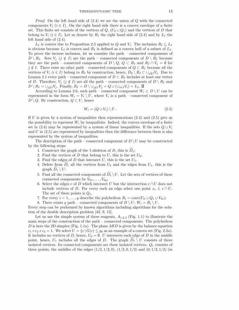
Let us use the simple system of three reagents, A1,2,3 (Fig. 1.1) to illustrate themain steps of the construction of the path – connected components. The polyhedronD is here the 2D simplex (Fig. 1.1a). The plane AffD is given by the balance equationc1+c2+c3 = 1. We select U = {c |G(c) ≤ g0 as an example of a convex set (Fig. 2.2a).It includes no vertices of D, hence, U0 = ∅. U intersects each edge of D in the middlepoint, hence, U1 includes all the edges of D. The graph D1 \ U consists of threeisolated vertices. Its connected components are these isolated vertices. Q1 consists ofthree points, the middles of the edges (1/2, 1/2, 0), (1/2, 0, 1/2) and (0, 1/2, 1/2) (in

14 A. N. GORBAN

A1

A2 A3

c*

U={c|G(c)≤g0}

a)

W1`

W3 W2

c) A1

A2 A3

V3 V2

R1={c|c2,3≤1/2}

b) A1

A2 A3

V3 V2

Q={c|c1,2,3≤1/2} V1

d) A1

A2 A3

V3 V2

A1W1=R1\U

={c|c2,3≤1/2, G(c)>g0}

V1={c|c1>1/2}

Fig. 2.1. Construction of the path – connected components Wi of D\U for the simple example.(a) The balance simplex D, the set U and the path – connected components Wi; (b) The polyhedronQ = conv(U0 ∪ Q1) (2.3) (U0 = ∅, Q1 consists of the middles of the edges) and the connectedcomponents Vi of D \ Q: Vi = {c ∈ D | ci > 1/2}; (c) The set R1 = conv(U0 ∪ Q1 ∪ (D0 ∩ V1)); (d)The connected components W1 described by the inequalities (as R1 \ U (2.4)).

this example, the choice of these points is unambiguous, Fig. 2.2a).The polyhedron Q is a convex hull of these three points, that is the triangle given

in Aff(D) by the system of three inequalities c1,2,3 ≤ 1/2 (Fig. 2.2b). The connectedcomponents of D \Q are the triangles Vi given in D by the inequalities ci > 1/2. Inthe whole R

3, these sets are given by the systems of an equation and inequalities:

Vi = {c | c1,2,3 ≥ 0, c1 + c2 + c3 = 1, ci > 1/2} .

The polyhedron Ri is the convex hull of four points, the middles of the edges andthe ith vertex (Fig. 2.2c). In D, Ri is given by two linear inequalities, cj ≤ 1/2, j 6= i.In the whole R

3, these inequalities should be supplemented by the equation andinequalities that describe D:

Ri = {c | c1,2,3 ≥ 0, c1 + c2 + c3 = 1, cj ≤ 1/2 (j 6= i)} .

The path – connected components of D\U , Wi are described as Ri \U Fig. 2.2d):in D we get Wi = {c | cj ≤ 1/2 (j 6= i), G(c) > g0}. In the whole R

3,

Wi = {c | c1,2,3 ≥ 0, c1 + c2 + c3 = 1, cj ≤ 1/2 (j 6= i), G(c) > g0} .

Vi are convex sets in this simple example, therefore, it is possible to simplifyslightly the description of the components Wi and to represent them as Vi \ U :

Wi = {c | c1,2,3 ≥ 0, c1 + c2 + c3 = 1, ci > 1/2, G(c) > g0}

(or Wi = {c | ci > 1/2, G(c) > g0} in D).In the general case (more components and balance conditions), the connected

components Vi may be non-convex, hence, description of these sets by the systemsof linear equations and inequalities may be impossible. Therefore, in the generalsituations, we have to use Ri for description of Wi.

THERMODYNAMIC TREE 15

3. Construction of the thermodynamic tree.

3.1. Problem Statement. Let a real continuous function G be given in thebounded polyhedron D. We assume that G is strictly convex in D, i.e. the set (theepigraph of G)

epi(G) = {(x, g) |x ∈ D, g ≥ G(x)} ⊂ D × (−∞,∞)

is convex and for any segment [x, y] ⊂ D (x 6= y) G is not constant on [x, y]. Astrictly convex function on a bounded convex set has a unique minimizer. Let x∗ bethe minimizer of G in D and g∗ = G(x∗) is the corresponding minimal value.

The level set Sg = {x ∈ D |G(x) = g} is closed and the sublevel set Ug = {x ∈D |G(x) < g} is open in D (i.e. it is the intersection of an open set with D). Thesets Sg and D \ Ug are compact and Sg ⊂ D \ Ug.

A continuous path ϕ[0, 1] → D is admissible if the function G(ϕ(x)) does notincrease on [0, 1]. For x, y ∈ D, x � y (x precedes y) if there exists an admissiblepath ϕ[0, 1] → D with ϕ(0) = x and ϕ(1) = y. We define the equivalence: x ∼ y ifx � y and y � x.

Definition 3.1. The tree of G in D is the quotient space T = D/ ∼. We usethe notation π : D → D/ ∼ for the natural projection.

Let x, y ∈ D. According to Corollary 3.5 proven in the next subsection, anadmissible path from x to y in D exists if and only if π(y) ∈ [π(x∗), π(x)]. Therefore,to describe constructively the relation x � y in D we have to solve the followingproblems:

1. How to construct the thermodynamic tree T ?2. How to find an image π(x) of a state x ∈ D on the thermodynamic tree T ?3. How to describe by inequalities a preimage of a segment of the thermodynamic

tree, π−1([w, z]) ⊂ D (w, z ∈ T )?

3.2. Coordinates on the thermodynamic tree. We get the following lemmadirectly from the definitions.

Lemma 3.2. Let x, y ∈ D. x ∼ y if and only if G(x) = G(y)(= g) and x and ybelong to the same path – connected component of Sg.

The path – connected components of D \Ug can be numerated by the connected

components of the graph D1 \Ug. The following lemma allows us to apply this resultto the path – connected components of Sg.

Lemma 3.3. Let g > g∗, W1, . . . ,Wq are the path – connected components of

D \Ug and σ1, . . . , σp are the path – connected components of Sg. Then q = p and σi

may be enumerated on such a way that σi is the border of Wi in D.

Proof. G is continuous in D, hence, if G(x) > g then there exists a vicinity of xin D where G(x) > g. Therefore G(y) = g for every boundary point y of D \Ug in Dand Sg is the boundary of D \ Ug in D.

Let us define a projection θg : D \ Ug → Sg by the conditions: θg(x) ∈ [x, x∗]and G(θg(x)) = g. The function G(θg(x)) is strictly increasing continuous and convexfunction on the interval [x, x∗]. It depends continuously on x in the uniform metrics.Therefore, the solution to the equation G(y) = g on [x, x∗] exists and continuouslydepends on x ∈ D \ Ug.

The fixed points of the projection θg are elements of Sg. The image of each path– connected component Wi is a path – connected set. The preimage of every path –connected component σi is also a path – connected set. Indeed, let θg(x) ∈ σi andθg(y) ∈ σi. There exists a continuous path from x to y in D\Ug. It may be composed

16 A. N. GORBAN

from three paths: (i) from x to θg(x) along the line segment [x, θg(x)] ⊂ [x, x∗] thena continuous path in σi between θg(x) and θg(y) (it exists because σi is a path –connected component of Sg and it belongs to D \ Ug because Sg ⊂ D \ Ug) and,finally, from θg(y) to y along the line segment [θg(y), y] ⊂ [x∗, y]. Therefore, theimages of a path – connected component Wi is a path – connected components of Sg

that may be enumerated by the same index i, σi. This σi is the border of Wi in D.The equivalence class of x ∈ D is defined as [x] = {y ∈ D | y ∼ x}. Let W (x) be

a path – connected component of D \ Ug (g = G(x)) for which θg(W (x)) = [x]. Dueto Lemma 3.3 such a component exists and

W (x) = {y ∈ D | y � x} . (3.1)

Let us define a one-dimensional continuum Y that consists of pairs (g,M) where

g∗ ≤ g ≤ gmax andM is a set of vertices of a connected component of D1\Ug. For each(g,M) the fundamental system of neighborhoods consists of sets Vρ = {(g+ γ,M ′) ∈Y | |γ| < ρ, M ′ ⊆M} (ρ > 0).

Let us define the preorder structure on Y: (g,M) � (g′,M ′) if g ≥ g′ andM ⊇M ′.

Proposition 3.4. Y is a homeomorphic image of T with preservation of pre-

order.

Proof. Let us consider the mapping φ : D → Y: x 7→ (G(x),W (x) ∩ D0).According to Lemmas 3.3, 3.1 and Proposition 2.4, the equivalent points x map tothe same pair (g,M) and non-equivalent points map to different pairs (g,M). Letus define the preorder structure on Y: (g,M) � (g′,M ′) if g ≥ g′ and M ⊇ M ′.For any x, y ∈ D, x � y if and only if φ(x) � φ(y). The fundamental systemof neighborhoods in Y may be defined using this preorder. Let us say that (g,M)is compatible to (g′,M ′) if (g′,M ′) � (g,M) or (g,M) � (g′,M ′)}. Then Vρ ={(g′,M ′) ∈ Y | |γ − γ′| < ρ, (g′,M ′) is compatible to (g,M)} (ρ > 0). So, Y has thesame preorder and topological structure as T .

Y can be considered as a coordinate system on T . Each point is presented as apair (g,M) where g∗ ≤ g ≤ gmax and M is a set of vertices of a connected component

of D1 \ Ug. The map φ is the coordinate representation of the canonical projectionπ : D → T . Now, let us use this coordinate system and the proof of Proposition

Corollary 3.5. An admissible path from x to y in D exists if and only if

π(y) ∈ [π(x∗), π(x)] .

Proof. Let there exists an admissible path from x to y in D, ϕ[0, 1] → D. Thenπ(x) � φ(y) in T . Let π(x) = (G(x),M) in coordinates Y. For any v ∈ M , π(y) ∈[π(x∗), π(v)] and π(x) ∈ [π(x∗), π(v)].

Assume now that π(y) ∈ [π(x∗), π(x)] and π(x) = (G(x),M). Then for anyπ(x) = (G(x),M) the admissible path from x to y in D may be constructed asfollows. Let v be a vertex of D for which π(v) = v. The straight line interval [x∗, v]includes a point x1 with G(x1) = G(x) and y1 with G(y1) = G(y). Coordinates ofπ(x1) and π(x) in Y coincide as well as coordinates of π(y1) and π(y). Therefore,x ∼ x1 and y ∼ y1. The admissible path from x to y in D may be constructedas sequence of three paths: first, a continuous path from x to x1 inside the path –connected component of SG(x)) (Lemma 3.2), then from x1 to y1 along a straight lineand after that a continuous path from y1 to y inside the path – connected componentof SG(y).

THERMODYNAMIC TREE 17

To describe the space T in coordinate representation Y , it is necessary to findthe connected components of the graph D1 \Ug for each g. First of all, this function,

g 7→ the set of connected components of D1 \ Ug ,

is piecewise constant. Secondly, we do not need to solve at each point the rather dif-ficult problem of the construction of the connected components of the graph D1 \ Ug

“from scratch”. The problem of the parametric analysis of these components as func-tions of g appears to be much simpler. Let us represent the solution of this problem.At the same time, this is the method for the construction of the thermodynamic treein coordinates (g,M).

3.3. Algorithm for construction of the thermodynamic tree. To con-struct the thermodynamic tree we need the following information: the graph D1 ofthe 1-skeleton of the balance polyhedron D labeled by the values of G. Each vertex vis labeled by the value γv = G(v) and each edge e = (v, w) is labeled by the minimalvalue of G on the segment [v, w] ⊂ D, ge = min[v,w]G(x). We need also the minimalvalue g∗ = minD{G(x)} because the root of the tree is (g∗, D0).

The convex function G achieves its local maxima in D only in vertices. Thevertex v is a (local) maximizer of g if ge < γv for each edge e that includes v. Theleaves of the thermodynamic tree are pairs (γv, {v}) for the vertices that are the localmaximizers of G.

Let us enumerate the vertices and the edges of D1 in order of the correspondentγv and ge: γv1

≥ γv2≥ . . . and ge1

≥ ge2≥ . . .. Some of the numbers γvi

, gejmay

coincide. Let there be l different numbers among them: a1 > a2 > . . . > al, whereeach ak belongs to {γvi

} or to {gej}.

The set of connected components of D1 \Ug is the same for all g ∈ (ai+1, ai]. For

g ∈ [g∗, al] the graph D1 \ Ug includes all the vertices and edges D1 and, hence, it isconnected for this segment. Let us take, formally, al+1 = g∗.

Let us construct the connected components of the graph D1\Ug starting from themaximal value of G: a1 = maxx∈D1

G(x). The function G is strictly convex, hence,a1 = γv for a set of vertices A1 ⊂ D0 but it is impossible that a1 = ge for an edge e.

For an interval (a2, a1] the connected components of D1 \Ug are the one-elementsets {v} for v ∈ A1.

Let Ai be the set of vertices v ∈ D0 with γv = ai and let Ei be the set of edgesof D1 with ge = ai (i = 1, . . . , l). Let Li = {M i

1, . . . ,Miki} be the set of the connected

components of D1 \ Ug for g ∈ (ai, ai−1] (i = 1, . . . , l) represented by the sets ofvertices M i

j .Assume that Li−1 is given. Let us find the set Li of connected components of

D1 \ Ug for g = ai (and, therefore, for g ∈ (ai+1, ai]).First of all, we add to the set Li−1 = {M i−1

1 , . . . ,M i−1ki−1

} the one-element sets {v}

for all v ∈ Ai. We will denote this auxiliary set of sets as L0 = {M1, . . . ,Mq}, whereq = ki−1 + |Ai|. Secondly, let us enumerate the edges from Ei in an arbitrary order:

e1, . . . , e|Ei|. For each k = 0, . . . , |Ei| we will create an auxiliary set of sets Lk by the

union of some of elements of L0. Let Lk−1 be given and ek connects the vertices v

and v′. If v and v′ belong to the same element of Lk−1 then Lk = Lk−1. If v and v′

belong to the different elements of Lk−1, M and M ′, then Lk is produced from Lk−1

by the union of M and M ′:

Lk = Lk \ {M} \ {M ′} ∪ {M ∪M ′}

18 A. N. GORBAN

D

[ES]

[S]

bE [E]=0

bS

bS

E, P

ES, P

E, S

ES, S a) bS>bE

[ES]

[S]

[E]=0 bS=bE

bS

D

E, P

ES

E, S

b) bS=bE

D1 D1

bS

[ES]

[S]

[E]=0 bE

bS

D

E, P

E, ES

E, S

c) bS<bE

D1

Fig. 3.1. The balance polygon D on the plane with coordinates [S] and [ES] for the four–component enzyme–substrate system S, E, ES P with two balance conditions, bS = [S]+[ES]+[P ] =const and bE = [E] + [ES] = const.

bO

bH

bH>2bO

bH=2bO

2bO>bH>bO

bH=bO

bH<bO

H2, OH

H2, O

H2, H2O

H, H2O

H, O

H, OH

H2, O2

H, O2

H2, OH

H2, O

H2O

H, O

H, OH

H2, O2

H, O2

H2, OH

H2, O

O2, H2O

O, H2O

H, O

H, OH

H2, O2

H, O2

H2O, OH

OH

H2, O

O2, H2O

O, H2O

H, O

H2, O2

H, O2

O, OH

O2, OH

O2, H

O2, H2O

O, H2O

H, O

O2, H2

O, H2

a)

b) c)

d)

e)

Fig. 3.2. The graph D1(b) of the one-skeleton of the balance polyhedron for the six-componentsystem, H2, O2, H, O, H2O, OH, as a piece-wise constant function of b = (bH, bO). For each vertexthe components are indicated which have non-zero concentrations at this vertex.

(we delete elements M and M ′ from Lk−1 and add a new element M ∪M ′). The set

Li of connected components of D1 \ Ug for g = ai is L|Ei|.

The described algorithm gives us the sets of connected components of D1 \Ug forall g and, therefore, we get the tree T . The descent from the higher values of G allowsus to avoid the solution of the computationally expensive problem of the calculationof the connected components of a graph.

4. Chemical kinetics: examples.

4.1. Skeletons of the balance polyhedra. In chemical kinetics, the variableNi is the amount of the ith component in the system. The balance polyhedron Dis described by the positivity conditions Ni ≥ 0 and the balance conditions (1.1)bi(N) = const (i = 1, . . . ,m). Under the isochoric (the constant volume) conditions,the concentrations ci also satisfy the balance conditions and we can construct the

THERMODYNAMIC TREE 19

H2, OH

H2, O

H2, H2O

H, H2O

H, O

H, OH

H2, O2

H, O2

H2, OH

H2, O

H2O

H, O

H, OH

H2, O2

H, O2

H2, OH

H2, O

O2, H2O

O, H2O

H, O

H, OH

H2, O2

H, O2

H2O, OH

a)

H2, OH

H2, O

O2, H2O

O, H2O

H, O

H, OH

H2, O2

H, O2

H2O, OH OH

H2, O

O2, H2O

O, H2O

H, O

H2, O2

H, O2

O, OH

O2, OH

O2, H

O2, H2O

O, H2O

H, O

O2, H2

O, H2

b)

Fig. 4.1. Transformations of the graph D1(b) with changes of the relation between bH and bO:(a) transition from the regular case bH > 2bO to the regular case 2bO > bH > bO through the singularcase bH = 2bO, (b) transition from the regular case 2bO > bH > bO to the regular case bH < bOthrough the singular case bH = bO.

balance polyhedron for concentrations. Sometimes, the balance polyhedron is calledthe reaction simplex with some abuse of language because it is not obligatory a simplexwhen the number m of the independent balance conditions is greater than one.

The graph D1 depends on the values of the balance functionals bi = bi(N) =∑nj=1 a

jiNj . For the positive vectors N , the vectors b with coordinates bi = bi(N)

form a convex polyhedral cone in Rm. Let us denote this cone by Λ. D1(b) is a piece-

wise constant function on Λ. Sets with various values on this function are cones.They form a partition of Λ. Analysis of this partition and the corresponding valuesof D1 can be done by the tools of linear programming [20]. Let us represent severalexamples.

In the first example, the reaction system consists of four components: the sub-strate S, the enzyme E, the enzyme-substrate complex ES and the product P . weconsider the system under constant volume. We denote the concentrations by [S],[E], [ES] and [P ]. There are two balance conditions: bS = [S] + [ES] + [P ] = constand bE = [E] + [ES] = const.

For bS > bE the polyhedron (here the polygon) D is a trapezium (Fig. 3.1a).Each vertex corresponds to two components that have non-zero concentrations in thisvertex. For bS > bE there are four such pairs, (ES, P ), (ES, S), (E], P ) and (E,S).For two pairs there are no vertices: for (S, P ) the value bE is zero and for (ES,E) itshould be bS < bE . When bS = bE , two vertices, (ES, P ) and (ES, S), transform intoone vertex with one non-zero component, ES, an the polygon D becomes a triangle

20 A. N. GORBAN

H2, OH

H2, O2

H, O2

H, OH

H, O

H2, O H2O

H2, HO2 H2, H2O2

H, HO2 H, H2O2

Fig. 4.2. The graph D1 for the eight-component system, H2, O2, H, O, H2O, OH, H2O2, HO2

for the stoichiometric mixture, bH = 2bO. The vertices that correspond also to the six-componentmixture are distinguished by bold font.

(Fig. 3.1b). When bS < bE then D is also a triangle and a vertex ES transforms inthis case into (ES,E) (Fig. 3.1c).

For the second example, we select a system with six components and two balanceconditions: H2, O2, H, O, H2O, OH;

bH = 2NH2+NH + 2NH2O +NOH ,

bO = 2NO2+NO +NH2O +NOH .

The cone Λ is a positive octant on the plane with the coordinates bH, bO. Thegraph D1(b) is constant in the following cones in Λ (bH, bO > 0): (a) bH > 2bO, (b)bH = 2bO, (c) 2bO > bH > bO, (d) bH = bO and (e) bH < bO (Fig. 3.2).

The cases (a) bH > 2bO, (c) 2bO > bH > bO, and (e) bH < bO (Fig. 3.2) areregular: there are two independent balance conditions and for each vertex there areexactly two components with non-zero concentration. In case (a) (bH > 2bO), ifbH → 2bO then two regular vertices, H2, H2O and H, H2O, join in one vertex (case(b)) with only one non-zero concentration, H2O (Fig. 4.1a). This vertex explodes inthree vertices O, H2O; O2, H2O and H2O, OH, when bH becomes smaller than 2bO(case (c), 2bO > bH > bO) (Fig. 4.1a).

Analogously, in the transition from the regular case (c) to the regular case (e)through the singular case (d) (bH = bO) three vertices join in one, 0H that explodesin two (Fig. 4.1b).

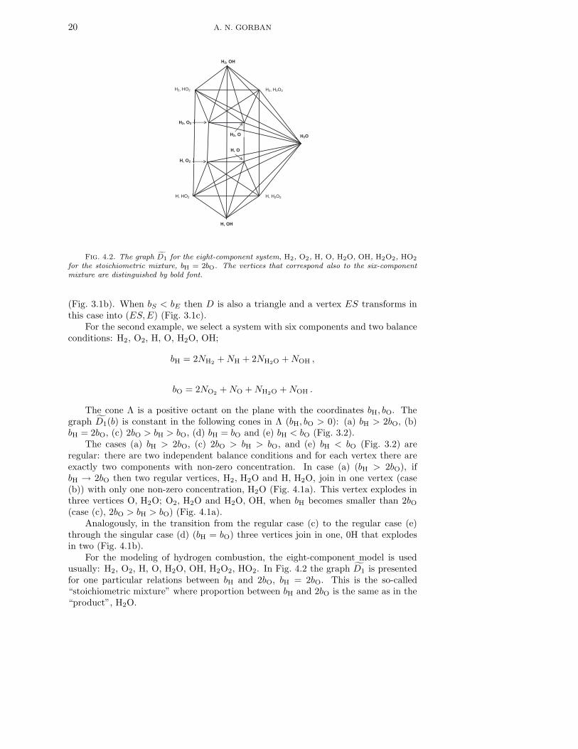
For the modeling of hydrogen combustion, the eight-component model is usedusually: H2, O2, H, O, H2O, OH, H2O2, HO2. In Fig. 4.2 the graph D1 is presentedfor one particular relations between bH and 2bO, bH = 2bO. This is the so-called“stoichiometric mixture” where proportion between bH and 2bO is the same as in the“product”, H2O.

THERMODYNAMIC TREE 21

v4

v3

v2

v1 v4

v3

v3

v3 v2

v1

γ1

γ2

g1

γ3

g2

γ4

g3

g4

g*

v1

v2

v1

v2

v1

v2

v1

v2

2

v1

v4

v4v3

v2

v1

ES, S

E, S

ES, P

E, P

c*

E, P

ES, P

E, S

ES, S

E

v2

v1 v3

P

v4

e1

e2

e4

e3

γ1>γ2>g1>γ3>g2>γ4>g3>g4

G

Fig. 4.3. The thermodynamic tree for the four–component enzyme–substrate system S, E, ESP (Fig. 3.1) with excess of substrate: bS > bE (case (a)). The vertices and edges are enumeratedin order of γv and ge (starting from the greatest values). The order of these numbers is repre-

sented in Fig. On the right, the graphs D1 \ Ug are depicted. The solid bold line on the tree isthe thermodynamically admissible path from the initial state E, S (enzyme plus substrate) to theequilibrium.

4.2. Examples of the thermodynamic tree. In this section, we representstwo example of the thermodynamic tree. First, let us consider the trapezium (Fig. 3.1a).Let us select the order of numbers γv and ge according to Fig. 4.3. The vertices andedges are enumerated in order of γv and ge (starting from the greatest values). Thetree is presented in Fig. 4.3.

On the right, the graphs D1 \ Ug are depicted for all intervals (ai−1, ai]. For(γ2, γ1] it is just a vertex v1. For (g1, γ2] it consists of two disjoint vertices, v1 andv2. For (γ3, g1] these two vertices are connected by an edge. On the interval (g2, γ3]

the graph D1 \ Ug is an edge (v1, v2) and an isolated vertex v3. On (γ4, g2] all threevertices v1, v2 and v3 are connected by edges. For (g3, γ4] the isolated vertex v4 is

added to the graph D1 \ Ug. For g ≤ g3 the graph D1 \ Ug includes all the verticesand is connected.

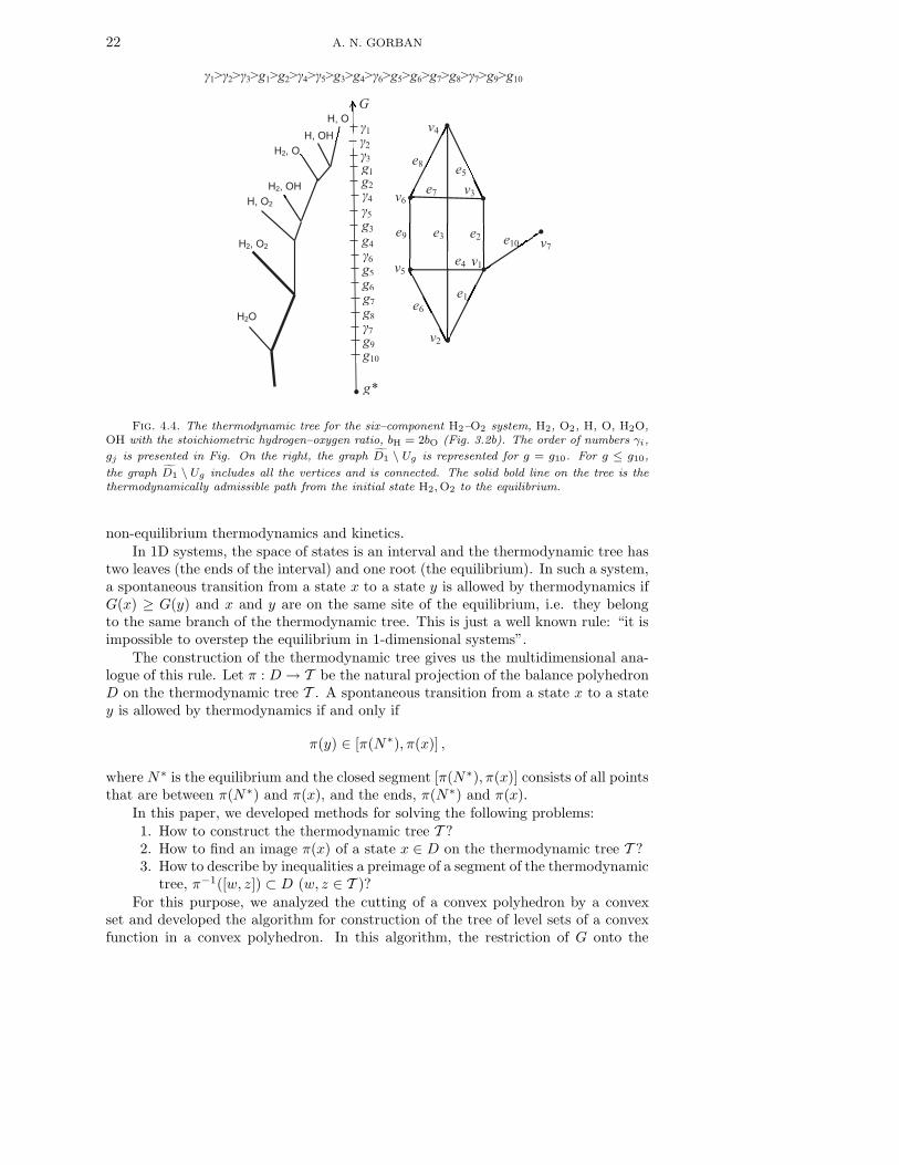
For the second example (Fig. 4.4) we selected the six-component system (Fig. 3.2)with the stoichiometric hydrogen–oxygen ratio, bH = 2bO. The selected order ofnumbers γi, gj is presented in Fig. 4.4.

5. Conclusion. The thermodynamic tree is a tool to answer the question: isthere a continuous path between two states, along which the conservation laws hold,the concentrations remain non-negative and the relevant thermodynamic potential G(Gibbs energy, for example) monotonically decreases? This question arises often in

22 A. N. GORBAN

v1

v2

v3

v4

v5

v6

v7

e1

e2 e3

ve4

e5

e6

e7

e8

e9 e10

γ1

γ3 γ3

g1

γ4

g3

γ6 γ6

g5

g*

G

γ1>γ2>γ3>g1>g2>γ4>γ5>g3>g4>γ6>g5>g6>g7>g8>γ7>g9>g10

γ1

γ2

g1

g2 γ

γ5 g3

g4

g5

g6 g6

g7 g7

g8 g8

γ7 γ7

g9 g9

g10

H, O

H, OH

H2, O

H2, OH

H, O2

H2, O2

H2O

Fig. 4.4. The thermodynamic tree for the six–component H2–O2 system, H2, O2, H, O, H2O,OH with the stoichiometric hydrogen–oxygen ratio, bH = 2bO (Fig. 3.2b). The order of numbers γi,

gj is presented in Fig. On the right, the graph D1 \ Ug is represented for g = g10. For g ≤ g10,

the graph D1 \ Ug includes all the vertices and is connected. The solid bold line on the tree is thethermodynamically admissible path from the initial state H2, O2 to the equilibrium.

non-equilibrium thermodynamics and kinetics.In 1D systems, the space of states is an interval and the thermodynamic tree has

two leaves (the ends of the interval) and one root (the equilibrium). In such a system,a spontaneous transition from a state x to a state y is allowed by thermodynamics ifG(x) ≥ G(y) and x and y are on the same site of the equilibrium, i.e. they belongto the same branch of the thermodynamic tree. This is just a well known rule: “it isimpossible to overstep the equilibrium in 1-dimensional systems”.

The construction of the thermodynamic tree gives us the multidimensional ana-logue of this rule. Let π : D → T be the natural projection of the balance polyhedronD on the thermodynamic tree T . A spontaneous transition from a state x to a statey is allowed by thermodynamics if and only if

π(y) ∈ [π(N∗), π(x)] ,

where N∗ is the equilibrium and the closed segment [π(N∗), π(x)] consists of all pointsthat are between π(N∗) and π(x), and the ends, π(N∗) and π(x).

In this paper, we developed methods for solving the following problems:1. How to construct the thermodynamic tree T ?2. How to find an image π(x) of a state x ∈ D on the thermodynamic tree T ?3. How to describe by inequalities a preimage of a segment of the thermodynamic

tree, π−1([w, z]) ⊂ D (w, z ∈ T )?For this purpose, we analyzed the cutting of a convex polyhedron by a convex

set and developed the algorithm for construction of the tree of level sets of a convexfunction in a convex polyhedron. In this algorithm, the restriction of G onto the

THERMODYNAMIC TREE 23

1-skeleton of D is used. This finite family of convex functions of one variable includesall necessary information for analysis of the tree of the level sets of the convex functionG of many variables.

Let us now formulate two more problems that also need to be solved:

• To find the maximal and the minimal value of any linear function f in a classof thermodynamic equivalence;

• To evaluate the maximum and the minimum of dG/dt in any class of ther-modynamic equivalence: −σ ≤ dG/dt ≤ −σ ≤ 0.

For any w ∈ T , the solution of the first problem allows us to find an interval ofvalues of any linear function of state in the corresponding class of thermodynamicequivalence. We can use the results of Sec. 2.2 to reformulate this problem as theconvex programming problem.

The second problem gives us the possibility to consider dynamics of relaxationon T . On each interval on T we can write

−σ(g) ≤dg

dt≤ −σ(g) ≤ 0 , (5.1)

where the functions σ(g), σ(g) ≥ 0 depend on the interval on T .

This differential inequality (5.1) will be a tool for the study of the dynamics ofrelaxation and may be considered as a reduced kinetic model that substitutes dynam-ics on the d-dimensional balance polyhedron D by dynamics on the one-dimensionaldendrite.

The problem of the construction of the reduced model (5.1) is closely related tothe following problem [53]: “Can one establish a lower bound on the entropy produc-tion, in terms of how much the distribution function departs from thermodynamicalequilibrium?” In 1982, C. Cercignani [8] proposed a simple linear estimate for σ(g)for the Boltzmann equation (Cercignani’s conjecture). After that, these estimateswere studied and improved by many authors [10, 7, 52, 53] and now the state of artachieved for the Boltzmann equation gives us some hints how to create the relaxationmodel (5.1) on the thermodynamic tree for the general kinetic systems. This will bethe next step in the study of the thermodynamic trees.

REFERENCES

[1] G. M. Adelson-Velskii, A. S. Kronrod, About level sets of continuous functions with partialderivatives, Dokl. Akad. Nauk SSSR, 49 (4) (1945), pp. 239–241

[2] P. M. Alberti, B. Crell, A. Uhlmann, C. Zylka, Order structure (majorization) and irre-versible processes, in Vernetzte Wissenschaften–Crosslinks in Natural and Social Sciences,P. J. Plath, E.-Chr. Hass, eds.; Logos Verlag, Berlin, Germany, 2008, pp. 281–290.

[3] P. M. Alberti, A. Uhlmann, Stochasticity and Partial Order – Doubly Stochastic Maps andUnitary Mixing; Mathematics and its Applications 9, D. Reidel Publ. Company, Dordrecht-Boston-London, 1982.

[4] A. D. Bazykin, Nonlinear dynamics of interacting populations, World Scientific Publishing:Singapore, 1998.

[5] V. I. Bykov, Comments on “Structure of complex catalytic reactions: thermodynamic con-straints in kinetic modeling and catalyst evaluation”, Ind. Eng. Chem. Res., 26 (1987),pp. 1943–1944.

[6] L. Boltzmann, Lectures on gas theory, U. of California Press, Berkeley, CA, 1964.[7] E. Carlen, M. Carvalho, Entropy production estimates for Boltzmann equations with phys-

ically realistic collision kernels, J. Statist. Phys., 74 (3-4) (1994), pp. 743–782.[8] C. Cercignani, H-theorem and trend to equilibrium in the kinetic theory of gases, Archiwum

Mechaniki Stosowanej, 34 (3) (1982), pp. 231–241.

24 A. N. GORBAN

[9] N. V. Chernikova, An algorithm for finding a general formula for nonnegative solutionsof system of linear inequalities, USSR Computational Mathematics and MathematicalPhysics, 5 (1965), pp. 228–233.

[10] L. Desvillettes, Entropy dissipation rate and convergence in kinetic equations. Comm. Math.Phys., 123 (4) (1989), pp. 687–702.

[11] A. Einstein, Strahlungs-Emission und -Absorption nach der Quantentheorie [=Emission andabsorption of radiation in quantum theory], Verhandlungen der Deutschen PhysikalischenGesellschaft, 18 (13/14) (1916). Braunschweig: Vieweg, pp. 318–323.

[12] M. Feinberg, D. Hildebrandt, Optimal reactor design from a geometric viewpoint–I. Uni-versal properties of the attainable region, Chem. Eng. Sci., 52 (1997), pp. 1637–1665.

[13] C. Filippi-Bossy, J. Bordet, J. Villermaux, S. Marchal-Brassely, C. Georgakis, Batchreactor optimization by use of tendency models, Comput. Chem. Eng., 13 (1989), pp. 35–47

[14] A. T. Fomenko, T. L. Kunii, eds., Topological Modeling for Visualization, Springer, Berlin,1997.

[15] K. Fukuda, A. Prodon, 1996. Double description method revisited, in Lecture Notes in Com-puter Science, vol. 1120. Springer-Verlag, Berlin, 1996, pp. 91–111.

[16] J. Gagneur, S. Klamt, Computation of elementary modes: a unifying framework and thenew binary approach, BMC Bioinformatics 2004, 5:175.

[17] D. Glasser, D. Hildebrandt, C. Crowe, A geometric approach to steady flow reactors:the attainable region and optimisation in concentration space, Am. Chem. Soc., 1987,pp. 1803–1810.

[18] A. N. Gorban, Invariant sets for kinetic equations, React. Kinet. Catal. Lett., 10 (1979),pp. 187–190.

[19] A. N. Gorban, Methods for qualitative analysis of chemical kinetics equations, in Numeri-cal Methods of Continuum Mechanics; Institute of Theoretical and Applied Mechanics:Novosibirsk, USSR, 1979; Volume 10, pp. 42–59.

[20] A. N. Gorban, Equilibrium Encircling. Equations of Chemical Kinetics and their Thermody-namic Analysis, Nauka Publ., Novosibirsk, 1984.

[21] A. N. Gorban, P. A. Gorban, G. Judge, Entropy: The Markov Ordering Approach, Entropy,12 (5) (2010), pp. 1145–1193.

[22] A. N. Gorban, B. M. Kaganovich, S. P. Filippov, A. V. Keiko, V. A. Shamansky, I. A.Shirkalin, Thermodynamic Equilibria and Extrema: Analysis of Attainability Regionsand Partial Equilibria, Springer, New York, NY, 2006.

[23] A. N. Gorban, G. S. Yablonskii, On one unused possibility in planning of kinetic experiment,Dokl. Akad. Nauk SSSR, 250 (1980), pp. 1171–1174.

[24] A. N. Gorban, G. S. Yablonskii, Extended detailed balance for systems with irreversiblereactions, Chem. Eng. Sci., 66 (2011), pp. 5388–5399.

[25] A. N. Gorban, G. S. Yablonskii, V. I. Bykov, Path to equilibrium. In Mathematical Problemsof Chemical Thermodynamics, Nauka, Novosibirsk, 1980, pp. 37–47 (in Russian). Englishtranslation: Int. Chem. Eng., 22 (1982), pp. 368–375.

[26] P. M. Gruber, J. M. Wills (eds.), Handbook of Convex Geometry, Volume A, North-Holland,Amsterdam, 1993.

[27] K. M. Hangos, Engineering model reduction and entropy-based Lyapunov functions in chem-ical reaction kinetics, Entropy, 12(4) (2010), pp. 772–797.

[28] D. Hildebrandt, D. Glasser, The attainable region and optimal reactor structures, Chem.Eng. Sci., 45 (1990), pp. 2161–2168.

[29] M. Hill, Chemical product engineering – the third paradigm, Comput. Chem. Eng., 33 (2009),pp. 947–953.

[30] F. Horn, Attainable regions in chemical reaction technique, in The Third European Symposiumon Chemical Reaction Engineering, Pergamon Press, London, UK, 1964, pp. 1–10.

[31] B.M. Kaganovich, A.V. Keiko, V.A. Shamansky, Equilibrium Thermodynamic Modeling ofDissipative Macroscopic Systems, Advances in Chemical Engineering, 39, 2010, pp. 1–74.

[32] S. Kauchali, W. C. Rooney, L. T. Biegler, D. Glasser, D. Hildebrandt, Linear program-ming formulations for attainable region analysis, Chem. Eng. Sci., 57 (2002), pp. 2015–2028.

[33] J. Klemela, Smoothing of multivariate data: density estimation and visualization, J. Wiley& Sons, Inc., Hoboken, NJ, 2009.

[34] A. N. Kolmogorov, Sulla teoria di Volterra della lotta per l’esistenza, Giornale Instituto Ital.Attuari, 7 (1936), pp. 74–80.

[35] F. J. Krambeck, Accessible composition domains for monomolecular systems, Chem. Eng.Sci., 39 (1984), pp. 1181–1184.

[36] A. S. Kronrod, On functions of two variables, Uspechi Matem. Nauk, 5(1) (1950), pp. 24-134.

THERMODYNAMIC TREE 25

[37] V. I. Manousiouthakis, A. M. Justanieah, L. A. Taylor, The Shrink-Wrap algorithm forthe construction of the attainable region: an application of the IDEAS framework, Comput.Chem. Eng., 28 (2004), pp. 1563–1575.

[38] R. M. May, W. J. Leonard, Nonlinear Aspects of Competition Between Three Species, SIAMJournal on Applied Mathematics, 29 (1975), pp. 243–253.

[39] C. McGregor, D. Glasser, D. Hildebrandt, The attainable region and Pontryagin’s maxi-mum principle, Ind. Eng. Chem. Res., 38 (1999), pp. 652–659.

[40] M. J. Metzger, D. Glasser, B. Hausberger, D. Hildebrandt, B. J. Glasser B.J. Use ofthe attainable region analysis to optimize particle breakage in a ball mill, Chem. Eng. Sci.,64, (2009), pp. 3766–3777.

[41] J. Milnor, Morse Theory, Princeton University Press, Princeton, NJ, 1963.[42] T. S. Motzkin, H. Raiffa, G. L. Thompson, R. M. Thrall, The double description method,

in Contributions of the Theory of Games II, H. W. Kuhn and A. W. Tucker, eds., Annalsof Mathematics, 8 (1953), Princeton University Press, Princeton, N.J., pp. 51–73.

[43] L. Onsager, Reciprocal relations in irreversible processes. I, Phys. Rev., 37 (1931), pp. 405–426.

[44] R. Peierls, Model-Making in Physics, Contemp. Phys., 21 (1980), pp. 3–17.[45] G. Reeb, Sur les points singuliers dune forme de Pfaff completement integrable ou dune fonc-

tion numerique, Comptes Rendus Acad. Sci. Paris 222 (1946), pp. 847–849.[46] S. Schuster, D. A. Fell, T. Dandekar, A general definition of metabolic pathways useful for

systematic organization and analysis of complex metabolic networks, Nat. Biotechnology,18 March (2000), pp. 326–332.

[47] R. Shinnar, Thermodynamic analysis in chemical process and reactor design, Chem. Eng.Sci., 43 (1988), pp. 2303–2318.

[48] R. Shinnar, C. A. Feng, Structure of complex catalytic reactions: thermodynamic constraintsin kinetic modeling and catalyst evaluation, Ind. Eng. Chem. Fundam., 24 (1985), pp. 153–170.

[49] K. Sigmung, Kolmogorov and population dynamics, in Kolmogorovs Heritage in Mathematics,

E. Charpentier; A. Lesne; N. K. Nikolski, eds.; Springer: Berlin, Germany, 2007; pp. 177–186.

[50] R. L. Smith, M. F. Malone, Attainable regions for polymerization reaction systems, Ind.Eng. Chem. Res., 36 (1997), pp. 1076–1084.

[51] W. Stuetzle, Estimating the cluster tree of a density by analyzing the minimal spanning treeof a sample, J. Classification 20(5) (2003), pp. 25–47.

[52] G. Toscani, C. Villani, Sharp entropy dissipation bounds and explicit rate of trend to equi-librium for the spatially homogeneous Boltzmann equation, Comm. Math. Phys., 203 (3)(1999), pp. 667–706.

[53] C. Villani, Cercignani’s conjecture is sometimes true and always almost true, Comm. Math.Phys., 234 (3) (2003), pp. 455–490.

[54] R. Wegscheider, Uber simultane Gleichgewichte und die Beziehungen zwischen Thermo-dynamik und Reactionskinetik homogener Systeme, Monatshefte fur Chemie / ChemicalMonthly, 32(8) (1911), pp. 849–906.

[55] G. S. Yablonskii, V. I. Bykov, A. N. Gorban, V. I. Elokhin, Kinetic models of catalyticreactions, Comprehensive Chemical Kinetics, Vol. 32, R. G. Compton, ed., Elsevier, Ams-terdam, 1991.

[56] M. Zarodnyuk, A. Keiko, B. Kaganovich, Elaboration of attainability region boundariesin the model of extreme intermediate states, Studia Informatica Universalis, 9 (2011),pp. 161–175.

[57] Ch. Zylka, A note on the attainability of states by equalizing processes, Theor. Chim. Acta,68 (1985), pp. 363–377.