thermoelectric materials for energy supply on a lunar base
TRANSCRIPT

M A S T E R T H E S I S
Thermoelectric materials
for energy supply on a
lunar base
Optimisation of the MgAgSb system
Laura Luhmann
September 2019 - September 2020
Thesis supervisors:
Dr. Aidan COWLEY, European Astronaut Centre
Dr. Johannes DE BOOR, German Aerospace Centre
Dr. Julien ZOLLINGER, EEIGM, Université de Lorraine

Thermoelectric materials for energy supply on a lunar base
Abstract
Even though most common thermoelectric generators are based on bismuth, tellurium, silicon or
germanium; the focus of this study is made on magnesium, silver and antimony in order to form
MgAgSb. Indeed, α-MgAgSb is a promising p-type material with the optimal temperature range fitting
the predicted operation conditions on a future lunar base (between 300 K and 600 K).
This project aims for the optimisation of MgAgSb by identifying the stoichiometry with the best
thermoelectric properties and the synthesis procedure leading to the least secondary phases. Indeed,
the material being defect rich, a stoichiometry of MgAg0.97Sb0.995 has been previously experimentally
identified as optimal, leading to a maximum figure of merit (zT) around 1.3 at 525 K without doping
elements [30].
The state of the art synthesis is a three-step process, consisting of a first high energy ball milling step
of only Mg and Ag, followed by a second milling of Mg, Ag and Sb. The final step involves a direct
sintering press. Nevertheless, each step can be tailored in order to optimise the thermoelectric
properties. Indeed, increasing the sintering duration of the second step was shown to be beneficial. As
a matter of fact, 20 min of sintering instead of 8 min led to only 2.0 wt. % of dyscrasite impurity in the
system. This reduction of secondary phases had a direct impact on the thermoelectric properties with a
maximum zT of 0.91 and an average zT of 0.78.
As the consolidation of MgAg is an important step before the addition of antimony to form MgAgSb,
the impact of a sintering step of MgAg between the two HEBM runs has been studied and led to a very
high Seebeck coefficient of 234 μV/K when MgAg was sintered at 500°C and a maximum zT of 0.85
for a 450°C MgAg sintering. Combining MgAg consolidation at 400°C with a longer sintering step of
MgAgSb (60 minutes) even led to a zTmax of 0.93 at 563 K.
Besides, as the secondary phases are a recurrent problem in MgAgSb synthesis, a high temperature
XRD experiment has been performed in order to determine if the impurity solubility is temperature
dependent. The experiment has revealed that the composition of the system does not seem to depend
on temperature, since no impurity precipitation/dissolution has been observed with a change in
temperature.
Keywords: Thermoelectric generator, MgAgSb, material optimisation, characterisation, secondary
phases.

Thermoelectric materials for energy supply on a lunar base
Résumé
Bien que la plupart des générateurs thermoélectriques soit composée de bismuth, tellure, silicium ou
germanium, ce projet s’appuie sur l’étude du magnésium, de l’argent et de l’antimoine pour former
MgAgSb. En effet, α-MgAgSb est un semi-conducteur de type p montrant ses propriétés optimales
dans un domaine de température adapté aux conditions opératoires attendues sur la future base lunaire
(entre 300 K et 600 K).
Ce projet a pour but d’optimiser le système MgAgSb en identifiant la stœchiométrie et le procédé de
synthèse menant aux meilleures propriétés thermoélectriques avec le moins de phases secondaires
possibles. Le matériau étant riche en défauts de structure, une stœchiométrie de MgAg0.97Sb0.995 a été
identifiée expérimentalement comme optimale, conduisant à un facteur de mérite (zT) maximal de 1,3
à 525 K sans dopage [30].
La synthèse actuelle consiste en trois étapes, la première utilisant un broyeur à billes de haute énergie
pour réduire Mg et Ag en poudre tout en produisant un alliage mécanique, la deuxième étant similaire
mais avec l’ajout de Sb. La dernière est une étape de frittage de la poudre, pour continuer la réaction.
Chaque étape peut ainsi être ajustée pour optimiser les propriétés thermoélectriques. En effet,
augmenter l’étape de frittage de 8 à 20 min a montré des effets bénéfiques, avec seulement 2,0 wt. %
d’impureté (dyscrasite) dans le système. Cette réduction de phases secondaires a ainsi augmenté les
propriétés thermoélectriques, menant à un zT maximal de 0,91 et un zT moyen de 0,78.
De plus, la consolidation de MgAg étant une étape importante avant l’ajout d’antimoine pour former
MgAgSb, l’impact d’une étape de frittage de MgAg entre les deux phases de broyage à haute énergie a
été étudié et a conduit à un coefficient de Seebeck très élevé de 234 μV/K pour un frittage à 500°C et
un zT maximal de 0,85 pour un frittage de MgAg à 450°C. Combiner la consolidation de MgAg à
400°C avec une étape de frittage de MgAgSb pendant 60 minutes a permis d’obtenir un zTmax de 0,93 à
563 K.
Enfin, les phases secondaires étant un problème récurrent dans la synthèse de MgAgSb, une
expérience de DRX à haute température a été menée pour déterminer si la solubilité des impuretés
dépend de la température. Celle-ci a révélé que la composition du système ne semble pas dépendre de
la température, puisque ni précipitation ou dissolution d’impuretés en fonction de la température n’a
été observée.
Mots-clés: Générateur thermoélectrique, MgAgSb, optimisation des matériaux, caractérisation, phases
secondaires.

Thermoelectric materials for energy supply on a lunar base
Acknowledgments
I would like to express my gratitude to my supervisors from DLR, ESA and EEIGM: Dr. Johannes de
Boor for pushing me forward and making a better scientist of me, Dr. Aidan Cowley for your help and
for really integrating me in the Spaceship team, Dr. Julien Zollinger for your support and your inputs
on my project. I want to thank Julia especially for your real implication, your useful comments and all
those great moments that we shared together in the office, with Antoine and Mohammad. Thank you
Nacho for your kind support and for transferring me your deep knowledge. I would like to thank
Przemek as well, not only for measuring my samples, but for being there for me every time I needed it.
Thanks to all my wonderful colleagues at DLR and ESA for making this year an amazing experience:
Prasanna, Vidushi, Elena, Diana, Gabriele, Eóin and Laura: keep being outstanding people. I would
also like to thank my friends that showed me unconditional support. Finally, heartful thanks to my
family who always believed in me even when I did not, for allowing me to follow my ambitions and
for being simply the best I could ask for.
“Never limit yourself because of others’ limited imagination; never limit others because of your own
limited imagination.”
– Mae Jemison, first African American female astronaut.

Thermoelectric materials for energy supply on a lunar base
Nomenclature
zT = Figure of merit
PF = Power Factor
S = Seebeck coefficient
σ = Electrical conductivity
κ = Thermal conductivity
HEBM = High Energy Ball Milling
DSP = Direct Sintering Press
HTSσ = High Temperature measurement of Seebeck and σ
LFA = Laser Flash Apparatus
SEM = Scanning Electron Microscope
SE = Secondary electrons
BSE = Backscattered electrons
XRD = X-Ray Diffraction
EDX = Energy-Dispersive X-ray spectroscopy
TE = Thermoelectric

Thermoelectric materials for energy supply on a lunar base
Table of Contents
Introduction ............................................................................................................................................. 1
1. Project context ..................................................................................................................................... 2
1.1. The European Space Agency (ESA) ....................................................................................... 2
1.2. The German Aerospace Centre (DLR) .................................................................................... 2
2. Theoretical background ....................................................................................................................... 3
2.1. Thermoelectric effects ............................................................................................................. 3
2.1.1. Seebeck effect .................................................................................................................. 3
2.1.2. Peltier effect .................................................................................................................... 4
2.1.3. Thomson effect ................................................................................................................ 5
2.2. Semiconductors ....................................................................................................................... 5
2.2.1. Generalities ...................................................................................................................... 5
2.2.2. Transport properties......................................................................................................... 7
2.3. Thermoelectric properties and performance ............................................................................ 9
2.3.1. Seebeck coefficient .......................................................................................................... 9
2.3.2. Electrical conductivity ................................................................................................... 10
2.3.3. Thermal conductivity..................................................................................................... 11
2.3.4. Figure of merit ............................................................................................................... 11
2.3.5. Single parabolic band model ......................................................................................... 12
2.4. MgAgSb: a promising p-type thermoelectric material .......................................................... 13
2.4.1. Physics of MgAgSb ....................................................................................................... 13
3. Materials and methods ....................................................................................................................... 20
3.1. Materials ................................................................................................................................ 20
3.2. Equipment ............................................................................................................................. 20
3.3. Synthesis process ................................................................................................................... 21
3.3.1. Previously used processes ............................................................................................. 21
3.3.2. Reference process in this study ..................................................................................... 21
3.4. HTSσ ..................................................................................................................................... 22
3.5. Laser Flash Apparatus ........................................................................................................... 25
3.6. Scanning Electron Microscope .............................................................................................. 26
3.7. X-ray diffraction .................................................................................................................... 28
4. Results and discussion ....................................................................................................................... 31
4.1. HEBM malfunction ............................................................................................................... 31

Thermoelectric materials for energy supply on a lunar base
4.1.1. Detection of the problem ............................................................................................... 31
4.1.2. Deterioration of the HEBM: replacement of some parts ............................................... 35
4.1.3. Speed monitoring........................................................................................................... 39
4.2. Effect of sintering duration on MgAgSb ............................................................................... 40
4.3. Consolidation of MgAg as a precursor .................................................................................. 44
4.4. Combination of MgAg consolidation and longer sintering of MgAgSb ............................... 51
4.5. Temperature dependence of impurity solubility .................................................................... 53
4.6. Discussion ............................................................................................................................. 56
5. Conclusions and perspectives ............................................................................................................ 60
Appendix ............................................................................................................................................... 62
References ............................................................................................................................................. 65

Thermoelectric materials for energy supply on a lunar base
List of Figures
Figure 1: Illustration of the Seebeck effect: a temperature difference between the heat source and the
heat sink causes the diffusion of charge carriers. The legs having opposite polarity, the generated
voltages add up. Figure taken from [10]. ................................................................................................ 4
Figure 2: Illustration of the Peltier effect: a current flow is responsible for the cooling of the top
junction, inducing a heat flow. Figure taken from [10]. .......................................................................... 5
Figure 3: Difference between insulators, metals and semiconductors. Figure taken from [12]. ............. 6
Figure 4: Undoped semiconductor. Figure adapted from [13]. ............................................................... 6
Figure 5: N-type doped semiconductor. Figure adapted from [13]. ........................................................ 7
Figure 6: P-type doped semiconductor. Figure adapted from [13]. ......................................................... 7
Figure 7: Band structure showing different curvatures for holes (blue) and electrons (red). Figure
adapted from [14]. ................................................................................................................................... 8
Figure 8: Evolution of Seebeck coefficient and electrical conductivity Sigma in the intrinsic and
extrinsic regimes. MgAgSb behaviour is considered as p-type. Figure taken from [18]. ..................... 10
Figure 9: Optimisation of zT through carrier concentration tuning. Here, the Seebeck coefficient is
referred to as α and not S. Figure taken from [17]. ............................................................................... 12
Figure 10: Representation of the crystal structures of (a) α-MgAgSb, (b) β-MgAgSb and (c) γ-
MgAgSb. The Mg-Sb sublattices are represented in yellow-orange and the Ag atoms located on the
Mg-Sb polyhedron sites are represented in light blue. Figure taken from [23]. .................................... 14
Figure 11: Tetragonal sublattice of α-MgAgSb showing the Mg4Sb4 hexahedron trapped in an Ag
atoms cage. Figure taken from [23]. ...................................................................................................... 14
Figure 12: Band structure of α-MgAgSb showing its indirect gap. Figure adapted from [24]. ............ 15
Figure 13: Ternary phase diagram for the system Magnesium-Silver-Antimony at 450°C. The dot
shows the composition that gives pure MgAgSb without secondary phases. Figure adapted from [25].
............................................................................................................................................................... 16
Figure 14: Thermoelectric figure of merit as a function of temperature for p- and n-type materials.
Figure taken from [31]. ......................................................................................................................... 18
Figure 15: Model of a Moon thermoelectric generator using regolith. Figure taken from [1]. ............. 18
Figure 16: Thermoelectric generator composed of p-type and n-type legs. TH is referring to the hot side
and TC to the cold side of the generator. Figure taken from [1]. ........................................................... 19
Figure 17: zT as a function of temperature for different thermoelectric materials (p-type). Figure
adapted from [32]. ................................................................................................................................. 19

Thermoelectric materials for energy supply on a lunar base
Figure 18: HEBM used during the first step of the synthesis. ............................................................... 20
Figure 19: Die containing MgAgSb with the thermocouple controlling the temperature. .................... 22
Figure 20: Temperature gradient between the two heaters, used for Seebeck coefficient measurement.
Figure taken from [37]. ......................................................................................................................... 23
Figure 21: Sample holder showing the thermocouples, springs and a sample pressed thanks to the
headless screw. Figure taken from [37]. ................................................................................................ 23
Figure 22: Typical heating and cooling curves obtained for Seebeck and σ between room temperature
and 290°C. ............................................................................................................................................. 24
Figure 23: Scheme of the LFA used in this project. Figure taken from [38]. ....................................... 25
Figure 24: Detection of the infrareds once the sample has been heated by the laser. Figure taken from
[39]. ....................................................................................................................................................... 25
Figure 25: Representation of (a) the pear-shaped interaction volume between the electron beam and
the sample [42] and (b) the formation of secondary electrons (on the left) and backscattered electrons
(on the right) [43]. ................................................................................................................................. 27
Figure 26: Representation of an XRD experiment: the X-ray beam is directed to the sample and the
diffracted waves are collected by the detector. Figure taken from [47]. ............................................... 28
Figure 27: Illustration of the incident waves being diffracted by the atomic planes of the sample.
Figure taken from [48]. ......................................................................................................................... 29
Figure 28: XRD spectrum of α-MgAgSb used as a reference. .............................................................. 29
Figure 29: Picture of the interior of the HEBM: the belt links the motor to the shaft, inducing the
motion of the jar containing the powder. ............................................................................................... 31
Figure 30: a) Reference sample before any HEBM problem (1119IRB14), b) Sb, Ag3Sb and Ag
impurities in the sample with the ongoing HEBM problem (1119IRB36) and c) after the belt has been
fixed (1119LLU02). Images taken using backscattered electrons......................................................... 32
Figure 31: Thermoelectric properties of 4 samples with the same experimental route, showing the
impact of the belt fixing (Reference before HEBM problem = 1119IRB14, HEBM before tightening =
1119IRB36, after tightening = 1119LLU02, same powder as after tightening = 1119LLU05). ........... 34
Figure 32: SEM images in backscattered electrons showing the impurities in the last sample before
changing parts (on the left) (1119LLU09) and after changing parts (on the right) (1120LLU04)........ 36
Figure 33: XRD pattern of (top) the last sample before changing the parts and (bottom) after changing
the parts. ................................................................................................................................................ 37
Figure 34: Comparison of the thermoelectric properties obtained before the HEBM problem (reference
= 1119IRB14), during the HEBM malfunction (first sample = 1119LLU06 – second sample produced
just after = 1119LLU09) and after changing the parts (1120LLU04). .................................................. 38
Figure 35: Set-up allowing the measurement of the HEBM speed: the reflective band put on the shaft
(on the left) reflects the tachometer’s laser (on the right). .................................................................... 39

Thermoelectric materials for energy supply on a lunar base
Figure 36: XRD patterns of (top) the sample after 20 min sintering (1120LLU10) and (bottom) after 8
min sintering (1120LLU04). ................................................................................................................. 41
Figure 37: SEM images of the sample after 20 min sintering (1120LLU10) (on the left) and after 8 min
sintering (1120LLU04) (on the right) in BSE. ...................................................................................... 42
Figure 38: Thermoelectric properties comparison between experimental samples sintered for 8 min
(1120LLU04) and 20 min (1120LLU10) as well as the literature reference sintered for 8 min. .......... 43
Figure 39: XRD patterns of (top) the sample with MgAg sintering at 500°C for 20 min followed by 8
min sintering of final MgAgSb (1120LLU15) and (bottom) the reference routine with only 8 min
sintering of final MgAgSb and no MgAg sintering (1120LLU04). ...................................................... 45
Figure 40: SEM images in BSE of the sample with MgAg sintering at 500°C (1120LLU15): (on the
left) with a 500 X magnitude and (on the right) with a 5 000 X magnitude. ........................................ 46
Figure 41: Thermoelectric properties comparison between the literature reference, the experimental
routine (8 min sintering of MgAgSb) (1120LLU04) and the sample obtained after sintering MgAg at
500°C (1120LLU15). ............................................................................................................................ 47
Figure 42: SEM images in BSE of a) the sample with MgAg sintering at 500°C (1120LLU15), b) the
sample with MgAg sintering at 450°C (1120LLU23) and c) the sample with MgAg sintering at 400°C
(1120LLU31)......................................................................................................................................... 49
Figure 43: Thermoelectric properties comparison between the literature reference and the samples
obtained after sintering MgAg at 500°C (1120LLU15), 450°C (1120LLU23) and 400°C
(1120LLU31)......................................................................................................................................... 50
Figure 44: SEM images of a) the sample after 8 min sintering (1120LLU31) and b) after 60 min
sintering (1120LLU32) in BSE. ............................................................................................................ 51
Figure 45: Thermoelectric properties comparison between experimental samples sintered for 8 min
(1120LLU31) and 60 min (1120LLU32) as well as the literature reference sintered for 8 min. .......... 52
Figure 46: High temperature XRD contour of (top) MgAgSb with α and β phases in presence and
(bottom) the major impurities found in MgAgSb: Ag3Sb (on the left) and Sb (on the right). Figure
adapted from [36]. ................................................................................................................................. 54
Figure 47: XRD patterns of the 3 cycles conducted on the sample (1120LLU01). Only α phase is
observed at all temperatures, indicating that the actual temperature remained below 300 °C. ............. 55
Figure 48: Closer look on a) the Sb impurity and b) dyscrasite. All cycles are shown to see the
influence of temperature on the impurities. ........................................................................................... 55
Figure 49: Contour of Sb (on the left) and Ag3Sb (on the right) impurities. ......................................... 56
Figure 50: zTaverage as a function of the total impurity content (Sb and Ag3Sb) for samples produced in
this project and the previous one. .......................................................................................................... 57
Figure 51: zTaverage as a function of a) the Ag3Sb content and b) the Sb content for samples produced in
this project and the previous one. .......................................................................................................... 58
Figure 52: zTmax and zTaverage for all samples produced during the previous project and this one. ........ 59
Thermoelectric materials for energy supply on a lunar base
List of Tables
Table 1: Advantages and disadvantages of thermoelectric generators, inspired by [31]. ..................... 17
Table 2: Impurity content comparison between the reference sample and the samples produced with a
malfunctioning HEBM. ......................................................................................................................... 33
Table 3: Impurity content comparison between the samples produced before and after changing the
parts. ...................................................................................................................................................... 36
Table 4: Impurity content comparison between 8 and 20 min sintering. .............................................. 41
Table 5: Impurity content after MgAg consolidation (and a second MgAgSb consolidation), compared
to the reference routine (with only one sintering step - for MgAgSb). ................................................. 45

1
Introduction
Around the world, space agencies are gathered to reach one main objective: be able to settle on the
Moon, and further beyond. Indeed, in the XXth century great improvements have been achieved in
space exploration, problems have been tackled thanks to women and men with great ambition and
considerable skills. From the first step on the Moon to the Hubble Space Telescope, without forgetting
the International Space Station, remarkable technologies have been developed and progress in the field
is not going to stop in the XXIst century. Reusable rockets have paved the way to even more
possibilities and engineers and scientists are determined to push the research forward and accomplish
more achievements, regarding other celestial bodies such as the Moon and Mars.
Indeed, even though the ISS has proved to be a major success both in terms of international
cooperation and scientific outcome, it will come to an end and the Moon gateway is the next step. In
the upcoming years, a lunar orbital platform will be constructed, in order to permit a crewed
exploration of the South Pole, leading to a lunar habitat where astronauts will be settled. However,
astronauts are going to face significant challenges on the Moon, from health impacts to nutritional
aspects or human/robotic collaboration. But one thing is for sure: they will need an energy source on
the Moon Village.
One might say that solar panels could appear as good energy suppliers for they are the main power
supplies for the ISS, satellites or probes. The problem lies in the eclipse time on the Moon. Indeed, the
ISS has only 45 minutes of absence of light during its 92 minutes Earth orbit. On the contrary, the
night time on the Moon can be considerably longer (about 14 days) so solar panels would not be able
to bring enough electricity. Thermoelectric generators could be a good alternative to provide energy to
the astronauts on a Moon base. They are indeed characterised by their thermoelectric effect, which
consists in the conversion of heat into electricity or vice-versa. A former member of Spaceship EAC
came up with the idea of designing a thermoelectric generator using the regolith that can be found on
the Moon. A solar concentrator could heat a block of regolith on one side, thus playing the role of the
heat source of the generator. On the other side, loose regolith would play its role as the cold sink. In
his work, he found out that when the hot part of the generator was at around 500 K, the heat loss was
acceptable for a 52 hours time frame, which corresponds to the night duration in the South Pole of the
Moon [1].
Thermoelectric generators have already been used in previous missions because they can furnish
power for long durations and with little maintenance needed. Moreover, they would be more suitable
than solar panels for lunar applications due to the dusty environment of the Moon. Indeed, the dust
could accumulate over the photovoltaic cells, preventing them to perform well due to light occlusion
[2]. Besides, the development of thermoelectrics for space application will also benefit humankind on
earth, since studies have revealed that more than 60 % of the worldwide energy is pointlessly lost,
mostly as heat waste, which could be used by such generators to provide sustainable energy [3].
Nevertheless, thermoelectric generators have been criticised for their lack of efficiency, leading
current material studies to focus on optimising their properties, which is the subject of this project.
Indeed, α-MgAgSb shows good thermoelectric properties between room temperature up to above 570
K, which is an asset since it covers the range of temperatures expected by the future Moon
thermoelectric generator. It also shows good mechanical properties, which needs to be taken into
account for the construction and operation of a module [4].

2
1
Project context
This project results from a collaboration between two important research centres located in Cologne:
the European Astronaut Centre (EAC) – part of the European Space Agency (ESA) – and the German
Aerospace Centre (DLR).
1.1. The European Space Agency (ESA)
Founded in 1975, the European Space Agency’s main mission is the peaceful exploration of space.
Their goal is to increase human knowledge with regard to Earth, the Solar system and more generally
the Universe. 22 member states constitute ESA Council, but other members are cooperating with
them, such as Canada or Slovenia. Even though ESA is focused on extending the limits of technology
and science in exploration, they might be known to the public for providing satellite-based services.
While ESA´s headquarters are in Paris, it has also different sites around Europe, like the ESA centre
for Earth Observation in Italy, the European Space Research and Technology Centre in the
Netherlands, the European Astronaut Centre in Germany and many more.
This internship took place in the European Astronaut Centre (EAC) in Cologne. It was established in
1990 in order to increase Europe’s influence in human space programmes. Indeed, EAC staff members
led by astronaut Frank de Winne are mainly focusing on astronaut selection, training, as well as
medical and psychological support, in order to prepare them for their future flight and journey on-
board the International Space Station (ISS).
However, EAC has also an important role in Space exploration due to a rather new initiative called
Spaceship EAC. Constituted by students, young graduates and research fellows, its goal is to unite
their different academic backgrounds to innovate and face the challenges of human exploration.
Spaceship EAC encourages its members to work on various low technology readiness level projects,
mainly focused on the lunar exploration. Many inspiring projects are being handled under six pillars:
advanced manufacturing, robotics, off-world living, space resources, disruptive technologies and
energy. The latter includes investigating ways of providing energy to the astronauts when they will be
on the Moon, using fuel cells or thermoelectric generators among others [5].
1.2. The German Aerospace Centre (DLR)
Resulting from the fusion of several aerospace research institutes, the German Aerospace Centre was
founded in 1969 and counts 20 locations in Germany. Its headquarters are in Cologne, where this
project took place. DLR is responsible for the design and implementation of the German Space
Program due to its high-technology infrastructures for research and innovation. Promoting German
research worldwide, its main focuses are aeronautics, space, transports, security, digitalisation and
energy.
This project was related to space and energy research and was conducted in the Thermoelectric
Materials and Systems department, belonging to the Materials Research institute. The department aims
to develop various thermoelectric materials with high efficiency. Indeed, skutterudites, magnesium-

3
silicides and MgAgSb are developed and tested, in order to be able to address various temperature
ranges for different technical applications. Moreover, those projects have also the goal of making
synthesis and fabrication compatible with industrial production processes, which is the reason why
students and research fellows are focused on finding an upscalable process for each of those systems
[6]. 2
Theoretical background
2.1. Thermoelectric effects
Thermoelectric materials involve the conversion between thermal and electrical energy based on
thermoelectric effects. Indeed, the Seebeck effect takes place when a temperature difference is
responsible for the diffusion of charge carriers in a material, thus generating an electric potential.
Electric currents inducing a heat flow are also considered as thermoelectricity and known as the Peltier
effect. [7].
These thermoelectric effects as well as the Thomson effect will be introduced below.
2.1.1. Seebeck effect
Even though Volta witnessed thermoelectricity in the 18th century, the Seebeck effect is named after
Thomas Johann Seebeck. Indeed, the latter noticed in 1821 that if a circuit was joined by two different
conducting materials (metals or semiconductors), the heating of one junction would induce an electric
current in the circuit, due to the temperature gradient between the junctions [8].
The Seebeck effect characterises the potential difference ΔV (in V) induced by the diffusion of charge
carriers due to a temperature gradient applied (ΔT = Thot - Tcold). Indeed, charge carriers (holes or
electrons) move from the hot side to the cold one and accumulate in the cold region, which results in
an electric potential difference, thus a current flow in the circuit when it is closed, see Figure 1.

4
Figure 1: Illustration of the Seebeck effect: a temperature difference between the heat source and the heat sink causes
the diffusion of charge carriers. The legs having opposite polarity, the generated voltages add up. Figure taken from
[10].
When a small temperature difference is applied, the Seebeck coefficient is defined as follows:
(2.1)
Where S is the Seebeck coefficient (in V.K-1
), which describes the magnitude of the effect.
Its sign can be positive or negative, depending on the type of majority charge carriers. Therefore, the
Seebeck coefficient is positive for p-type materials (where the majority charge carriers are holes) and
negative for n-type (where the majority charge carriers are electrons) [9].
2.1.2. Peltier effect
The Peltier effect is named after the French physicist Jean-Charles Peltier and takes place when an
electric current is applied to a thermoelectric couple. It is the somewhat reverse phenomenon of the
Seebeck effect: an electric current causes the heating or cooling of a junction made of different
conducting materials. One interesting aspect of the Peltier effect is that the direction of heat transfer is
tuned by the polarity of the current, which means that one can choose to make the junction absorb or
emit heat, taking into account the sign of the major charge carriers, see Figure 2. The Peltier effect is
used in electronic refrigerators and for precise temperature control [9][11].
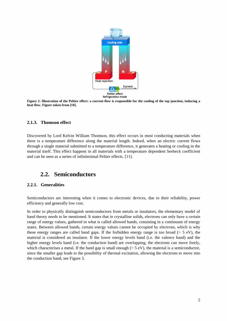
5
Figure 2: Illustration of the Peltier effect: a current flow is responsible for the cooling of the top junction, inducing a
heat flow. Figure taken from [10].
2.1.3. Thomson effect
Discovered by Lord Kelvin William Thomson, this effect occurs in most conducting materials when
there is a temperature difference along the material length. Indeed, when an electric current flows
through a single material submitted to a temperature difference, it generates a heating or cooling in the
material itself. This effect happens in all materials with a temperature dependent Seebeck coefficient
and can be seen as a series of infinitesimal Peltier effects. [11].
2.2. Semiconductors
2.2.1. Generalities
Semiconductors are interesting when it comes to electronic devices, due to their reliability, power
efficiency and generally low cost.
In order to physically distinguish semiconductors from metals or insulators, the elementary model of
band theory needs to be mentioned. It states that in crystalline solids, electrons can only have a certain
range of energy values, gathered in what is called allowed bands, consisting in a continuum of energy
states. Between allowed bands, certain energy values cannot be occupied by electrons, which is why
these energy ranges are called band gaps. If the forbidden energy range is too broad (> 5 eV), the
material is considered an insulator. If the lower energy levels band (i.e. the valence band) and the
higher energy levels band (i.e. the conduction band) are overlapping, the electrons can move freely,
which characterises a metal. If the band gap is small enough (< 5 eV), the material is a semiconductor,
since the smaller gap leads to the possibility of thermal excitation, allowing the electrons to move into
the conduction band, see Figure 3.

6
Figure 3: Difference between insulators, metals and semiconductors. Figure taken from [12].
Moreover, semiconductors can be defined by two different electric behaviours, i.e. intrinsic or
extrinsic. Pure undoped semiconductors are by definition intrinsic: no external elements are added to
the system and only internal charge carriers are considered. Thermal excitation is needed to give
enough energy to move the electrons from the valence band to the conduction band, since the
conduction is ensured by the exponential increase of free charge carriers with temperature. Indeed,
with increasing temperature, more and more electrons leave the valence band in order to join the
conduction band, leaving holes in the valence band. The electrons present in the conduction band are
now free to conduct electricity, as well as the holes left in the valence band, see Figure 4.
Figure 4: Undoped semiconductor. Figure adapted from [13].
For undoped semiconductors, the number of electrons in the conduction band is equal to the number of
holes in the valence band, which gives:
(2.2)
With nint and pint being the concentration (in m-3
) of respectively electrons and holes in the intrinsic
regime, EG the energy of the band gap (in eV), k and h respectively the Boltzmann and Planck
constants and m* the effective mass (in kg) that will be developed in the next section.
However, when doping is involved, semiconductors can exhibit both intrinsic and extrinsic behaviour,
depending on the conditions. Doping refers to the addition of a small quantity of foreign atoms in the

7
system. In the intrinsic regime (taking place at very low and high temperature), the charge carriers
coming from the host atoms are mainly responsible for the conduction. However, in the extrinsic
regime (at low temperature) the conduction is dominated by the charge carriers coming from the
dopants.
When it comes to dopants, two types of doping are possible: n- or p-type. N-type semiconductors
contain foreign atoms with a number of valence electrons higher than the host atoms’ number. N refers
to the negative charges added to the system. These electrons coming from the dopant are at a higher
energy level than the valence band and usually close to the conduction band. This means that the
temperature excitation needed to reach the conduction band and conduct electricity is rather low, as
seen in Figure 5.
Figure 5: N-type doped semiconductor. Figure adapted from [13].
P-type semiconductors contain foreign atoms with a number of valence electrons lower than the host
atoms’ number this time. In this case, the majority charge carriers are holes. The dopants create an
energy level just above the valence band. Again, thermal excitation will move some electron from the
valence band to reach this low energy level, leaving a hole in the valence band, which will contribute
to the electrical conduction, see Figure 6 [13].
Figure 6: P-type doped semiconductor. Figure adapted from [13].
2.2.2. Transport properties

8
As previously mentioned, charge carriers play an essential role in semiconductors and can be both
holes and electrons. This section focuses on the transport properties associated to these charge carriers,
which will help understand the related thermoelectric parameters.
Whether the semiconductor is n- or p-doped, it is essential to evaluate the density of the charge
carriers, also known as the carrier concentration respectively n or p (in cm-3
). Since thermoelectric
effects are depending on the diffusion of charge carriers, their concentration is closely linked to
thermoelectric properties. The density of charge carriers is also influenced by the material
composition. In p-type materials, holes have been considered above as the resulting absence of an
electron leaving the valence band to join the conduction band. They can also be internally produced by
vacancies in the crystallographic structure of the material, which is the case for MgAgSb. As a result,
these vacancies as well as potential impurities influence the carrier concentration.
The effective mass m* is defined as the mass a particle seems to have when it is responding to forces
applied. When it comes to band modelling, the effective mass depends on the type of charge carriers
(holes or electrons) and is linked to the local curvature of the band near the extremum of the valence
band (for holes) or the conduction band (for electrons), see Figure 7.
Figure 7: Band structure showing different curvatures for holes (blue) and electrons (red). Figure adapted from [14].
The effective mass also has an influence on the transport properties, because if the effective mass is
higher, charge carriers will move slower. [15].
Finally, another physical quantity influences the transports properties: the carrier mobility μ
(cm²/(V.s)). It characterises how fast charge carriers can move through the semiconductor when an
electric field is applied. However, the mobility of charge carriers is compromised by many
mechanisms encountered in the material. Indeed, impurities, grain boundaries or point defect
scattering can reduce the mobility. At high temperatures, scattering by acoustic phonons is usually the
dominant scattering mechanism for charge carriers.
Besides, at high temperatures, some effects are in competition with others. For example, if the
temperature is high, the thermal energy given to the charge carriers will cause intrinsic excitation,

9
which will increase the number of charge carriers that take part in the conduction. However there will
be more lattice vibrations, thus more phonon scattering and this will decrease the mobility [16].
2.3. Thermoelectric properties and performance
2.3.1. Seebeck coefficient
The Seebeck coefficient S is a material property and as it has been explained previously, it is linked to
the fact that charge carriers are conducting both electricity and heat. The electric field induced by the
diffusion of the charge carriers causes a voltage, called the Seebeck voltage.
The transport properties’ influence on the Seebeck coefficient can be expressed by a model of electron
transport taking the charge carrier concentration and the effective mass interconnection into account,
for metals or highly degenerate semiconductors. These are semiconductors with a high doping level
that makes them act rather like metals than semiconductors [17]:
(2.3)
With m* the effective mass and n the carrier concentration.
Finally, a material has a positive or negative S depending on its majority charge carriers. The Seebeck
coefficient for both types of carriers is thus calculated by an average weighted by their respective
electrical conductivity values (σe or σh):
(2.4)
The letters e and h referring respectively to the electrons or holes contribution.
For a constant majority carrier concentration, the difference between the number of majority and
minority charge carriers will influence the thermoelectric properties. At medium temperature, the
extrinsic regime takes place and the majority charge carriers have the lead role; there are way more
majority charge carriers than minority charge carriers, so the Seebeck will increase with temperature
according to equation 2.4. However, at high temperature, the influence of thermal excitation on
electron-hole pairs increases the role of the minority charge carriers: we are in the intrinsic regime.
The high amount of minority charge carries decreases the absolute Seebeck coefficient as and
have opposite signs in equation 2.4 [17].
This is represented on the p-doping curve in Figure 8, which relates to the behaviour of MgAgSb:

10
Figure 8: Evolution of Seebeck coefficient and electrical conductivity Sigma in the intrinsic and extrinsic regimes.
MgAgSb behaviour is considered as p-type. Figure taken from [18].
On this figure, it can also be seen that charge carriers not only affect the Seebeck coefficient but also
the electrical conductivity Sigma, which is developed below.
2.3.2. Electrical conductivity
The electrical conductivity σ is defined as a material’s capability to allow the transport of electric
charges. It is expressed in S.m-1
.
It is related to the mobility of charge carriers μ and their density n and given by the following equation
for a single carrier type:
(2.5)
When holes and electrons both contribute to the electrical conductivity, their contributions are added
up:
(2.6)
With n and μe referring to respectively the electron concentration and mobility and p and μh the hole
concentration and mobility. In semiconductors, a high electrical conductivity can usually be achieved
through doping to increase the carrier concentration.
Moreover, looking at the formulas, the influence of transport properties such as charge carrier
concentration and mobility is obvious. In Figure 8, the electrical conductivity is also represented and is
decreasing in the extrinsic regime and increasing in the intrinsic regime, contrary to the p-type
Seebeck. The decrease of electrical conductivity with temperature in the extrinsic regime is explained
by a reduced mobility, since the major charge carriers are taking the lead role, thus making the energy
levels very crowded on the one hand; on the other hand more phonons with higher energy scatter the
charge carriers, reducing the general mobility. However, when the temperature is increasing again,
additional charge carriers (electron-hole pairs) are created: we are in the intrinsic regime. So even if
the mobility is low due to a high amount of charge carriers, the increase in carrier concentration is
strong enough to increase the electrical conductivity, because more charge carriers participate to the
electrical conductivity.
To conclude this part, it seems important to insist on the influence of the transport properties on the
Seebeck coefficient and the electrical conductivity. Indeed, they can sometimes have opposite effects.
For example, increasing the carrier concentration is not beneficial to Seebeck but is a good solution to

11
increase the electrical conductivity. Moreover, a general competition lies between the mobility and the
charge carrier concentration, because increasing the concentration generally leads to a decrease in
mobility [18].
2.3.3. Thermal conductivity
The thermal conductivity κ is defined as the capability to transfer heat through a material. It is
expressed in W.m-1
.K-1
. Several sources are responsible for the thermal conductivity: elemental charge
carriers, electron-hole pairs and phonons. Charge carriers are responsible for the electronic thermal
conductivity κe, electron-hole pairs for the bipolar contribution κbi and the phonons for the lattice
thermal conductivity κlat. Phonons are referred to as quantised vibrations of the lattice, i.e. a collective
elastic excitation of atoms in condensed matter. This produces waves that can carry heat through the
crystal. The bipolar contribution comes from the electron-hole pairs that form at high temperature, in
the intrinsic regime. As a result, κ can be expressed as follows:
(2.7)
As κe is related to charge carriers, it can also be linked to the electrical conductivity σ through the
Wiedemann-Franz relation:
(2.8)
L0 being the Lorenz factor, which is usually taken constant for metals but can be expressed as a
function of the Seebeck coefficient for more accuracy in semiconductors [19]:
(2.9)
κlat depends on the contributions of phonons of all frequencies and can be calculated using the mean
free path of phonons, taking some phonon interactions into account. However, it is usually obtained by
subtracting κe from the total thermal conductivity, which is not totally accurate at high temperature,
since there is still the bipolar contribution left in the equation:
(2.10)
However, as the thermoelectric performance is usually enhanced with low thermal conductivity κ but
high electrical conductivity σ, experiments tend to focus on reducing κlat instead of κe, this one being
linked to σ. In order to do so, phonon scattering is interesting and can be achieved by grain boundaries
scattering (tailoring the grains size or the grain boundary type), point defect scattering or even
interface scattering using a multilayer system composed of thin films [18].
2.3.4. Figure of merit
The evaluation of the performance of thermoelectric devices is made with the efficiency η
(dimensionless). It gives an idea of the efficiency of the entire thermoelectric device and not only the
material and is given by equation 2.11:
(2.11)
Here Tc and Th are respectively the temperatures at the cold and hot sides of the device. ΔT is the
temperature difference between the two sides and ZT is the device figure of merit, taking into account
the temperature dependence of the materials properties in the considered temperature range [17].
Indeed, η depends on factors such as dimensions and contact resistance. ZT (in upper case to avoid any

12
confusion with the material zT) takes those other factors into account and is for this reason used in the
efficiency formula.
The material figure of merit zT is defined as follows:
(2.12)
with T the absolute temperature in K.
As all thermoelectric properties are combined in zT, a material performance for thermoelectric
applications can be evaluated by it. It is dimensionless and linked to all the thermoelectric quantities
developed above.
Another thermoelectric quantity is hidden in the figure of merit. Indeed, the product σS² is called the
power factor PF (in W.m-1
.K-2
). It reveals the maximal power output the material is able to reach. The
power factor can be optimised by tailoring the carrier concentration. To increase zT and have the best
performance, the materials need to have a high power factor and a low thermal conductivity. Usually,
zT values superior to 1 are desired.
Finally, Figure 9 shows the variation of all the thermoelectric properties as a function of carrier
concentration.
Figure 9: Optimisation of zT through carrier concentration tuning. Here, the Seebeck coefficient is referred to as α and not S. Figure taken from [17].
It is clear that increasing the carrier concentration has a positive effect on the thermal and electrical
conductivities; however it is detrimental for the Seebeck coefficient, thus for zT and PF. The power
factor reaches its maximum at a higher concentration than zT, which is explained by the fact that zT
also takes into account the thermal conductivity. Moreover, the optimal thermoelectric performances
are achieved by a carrier concentration in the range of 1019
to 1020
carriers per cm3 [17].
Finally, it confirms that the transport properties (mobility, effective mass and charge carrier
concentration) are not only linked together but also to the thermoelectric parameters. This explains
how hard it is to find the best thermoelectric properties, given that the transport properties have
usually opposite effects one with another.
2.3.5. Single parabolic band model

13
To understand transport properties of thermoelectric materials more deeply and improve them to get
better thermoelectric properties, some band structures models of semiconductors have been developed.
Indeed, some research has been focused on finding rather simple models to describe the behaviour of
the transport properties.
For highly doped semiconductors, the single parabolic band model can be used to represent the band
structures of n- and p-type thermoelectrics. It states that electronic properties are determined by a
single parabolic and rigid band, as its name suggests, which means that the effective mass m* does not
depend on the carrier concentration n and the band structure is independent of dopant substitution [20].
The carrier concentration n can then be calculated with the following equation:
(2.13)
with Fi(x) the Fermi integral of order i and η the reduced chemical potential linked to the experimental
Seebeck coefficient S by
(2.14)
Then, assuming that the effective mass is constant, it is possible to link the Seebeck coefficient to the
carrier concentration. Finally, the carrier concentration n being known, it is possible to find the
mobility μ, as they are linked through the electrical conductivity σ (equation 2.5).
This shows in what extend the single parabolic band model is useful, since it allows modelling and
analysing the thermoelectric transport properties. It also means that it plays an important role when it
comes to optimise the thermoelectric efficiency, by tailoring the transport parameters [21]. However,
the SPB model has some limitations because it is a simple model that only considers the major charge
carriers, that is why other models have been developed. For example, the one valence band + one
conduction band model takes into account the influence of minor charge carriers as well and the two
parabolic valence band model assumes non-rigid bands with a temperature dependent gap.
2.4. MgAgSb: a promising p-type thermoelectric material
2.4.1. Physics of MgAgSb
Crystallography
Even though the material studied in this project is generally referred to as MgAgSb, the most
interesting phase that gives the best thermoelectric properties is α-MgAgSb. Indeed, three different
crystal structures have been discovered for MgAgSb. From room temperature up to 563 K, the α-
MgAgSb phase is stable, then comes the intermediate β-MgAgSb phase stable up to 633 K. For
temperatures superior to 793 K only the γ-MgAgSb phase exists in equilibrium. For all phases, the Mg
and Sb atoms form Mg-Sb rocksalt-type sublattices (either distorted or undistorted) and the Ag atoms
are located on half of the Mg-Sb polyhedron sites [22]. A representation of the three structures can be
found in Figure 10.

14
Figure 10: Representation of the crystal structures of (a) α-MgAgSb, (b) β-MgAgSb and (c) γ-MgAgSb. The Mg-Sb
sublattices are represented in yellow-orange and the Ag atoms located on the Mg-Sb polyhedron sites are represented
in light blue. Figure taken from [23].
As the α-MgAgSb phase is the phase of interest in this project, its crystallographic structure will be
developed here. At room temperature, a diffraction pattern of α-MgAgSb has determined its structure
as tetragonal with a space group. The lattice parameters are a = b = 9.1631 Å and c = 12.701 Å.
As previously mentioned, the crystallographic structure consists of a distorted Mg-Sb rocksalt-type
lattice, which has been rotated by 45° around the z axis. The Ag atoms are filling half of the Mg-Sb
pseudo cubes. This results in a Mg4Sb4 hexahedron trapped in a cage formed by different Ag atoms, as
it can be seen in Figure 11.
Figure 11: Tetragonal sublattice of α-MgAgSb showing the Mg4Sb4 hexahedron trapped in an Ag atoms cage. Figure
taken from [23].
Ag1 atoms are situated in the corners of the tetragon, Ag2 are on the edges of the c’ axis and Ag3
atoms on the edges of a’ and b’ axes. This results in chemical bonds with different lengths between
Ag-Ag atoms, inducing weaker bonds than in the more stable γ-MgAgSb. However, weaker bonds
might have a positive impact on the thermal conductivity. Indeed, the larger unit cell of α-MgAgSb, as
well as the weak silver bonds result in strong phonon vibrations, lowering the lattice thermal
conductivity. Moreover, even though the cell parameters of α-MgAgSb show linear thermal
expansion, they have different thermal expansion coefficients, leading to an anisotropic evolution of α-
MgAgSb with temperature [22].
β-MgAgSb has a tetragonal structure with space group . At medium temperatures the Mg
and Sb atoms of the β phase are forming a rocksalt lattice; however at higher temperature the lattice is
rather distorted. In the tetragonal structure, the silver atom distribution is rather layered and not three

15
dimensional like in the α phase. This increases the anisotropy of β-MgAgSb. The lattice parameters
are a = b = 4.4216 Å and c = 6.8923 Å.
The γ phase of MgAgSb has a half-Heusler structure, which makes it a more stable compound with an
equiatomic ternary intermetallic structure. It has a cubic structure with space group and its
lattice parameters are a = b = c = 6.6847 Å [23].
These differences in crystallographic structures lead to different densities, with 6.326 g.cm-3
for α-
MgAgSb, 6.258 g.cm-3
for β and 5.646 g.cm-3
for the γ phase.
Band Structure
In this project the synthesised α-MgAgSb is pure, has no doping elements involved and is considered
as a p-type material. Indeed, the p-type behaviour comes from Ag vacancies and Ag antisites (i.e. Ag
on Mg sites) that act as shallow acceptors. As a result, the major charge carriers in α-MgAgSb are
holes and not electrons [24].
Feng et al. calculated the band structure of α-MgAgSb, taking into account the underestimation of the
band gap obtained by previous methods [24]. They found that α-MgAgSb has a band gap of 0.32 eV
and a band structure constituted by an indirect gap. This is represented in Figure 12 by the conduction
band minimum near the Г point and the valence band maximum located between Z and A.
Figure 12: Band structure of α-MgAgSb showing its indirect gap. Figure adapted from [24].
Phase diagram
The ternary phase diagram for MgAgSb system is very complex and unfortunately not widely
investigated in literature, the last study dating from 1950 by B. R. T. Frost and G. V. Raynor [25].
The only isothermals available being at 450°C and 550°C, it has been decided to work with the one at
450°C because it is closer to the temperatures reached during the synthesis of α-MgAgSb. Indeed, a
similar behaviour might be expected for 300°C, i.e. the maximum temperature achieved during the
experiments. Figure 13 also indicates the secondary phases that might be formed during MgAgSb
synthesis.

16
Figure 13: Ternary phase diagram for the system Magnesium-Silver-Antimony at 450°C. The dot shows the
composition that gives pure MgAgSb without secondary phases. Figure adapted from [25].
It appears clearly that the region where the pure phase MgAgSb is obtained is very narrow since it is
centred around the 1:1:1 ratio of Mg:Ag:Sb and is represented by a dot. This explains how difficult it
is to form pure MgAgSb without secondary phases during the experimental synthesis, specifically
because some of those phases are very stable. Usually, the XRD analysis of the samples gives an idea
of which secondary phases are present and thus can give an indication of where the overall
composition of a sample is located on the phase diagram, in particular if equilibrium has been reached.
Knowing that, it is possible to tailor the atomic content of each of the elements in order to avoid some
secondary phases, considered as impurities.
State of the art MgAgSb
Many studies have been focused on finding the best thermoelectric properties of α-MgAgSb. Pure
(undoped) α-MgAgSb with a 1:1:1 ratio has shown great thermoelectric properties at room
temperature, with a Seebeck coefficient around 200 μV.K-1
, an average thermal conductivity of 0.8
W.m-1
.K-1
and an average electrical conductivity of 400 S.cm-1
. This led to a rather high maximal zT
value of 1.1 at 520 K [23].
In their discovery, Zhao et al. stated that two high energy ball milling steps (first Mg and Ag and then
MgAg with Sb) followed by hot pressing and annealing helped to get rid of impurities. Moreover, they
also brought to light the need of a composition deficient in Ag and Sb, such as MgAg0.97Sb0.99 in order
to increase the thermoelectric properties and get rid of impurities related to silver and antimony. For
MgAg0.97Sb0.99 they found a maximum zT around 1.2 at 450 K [26].
Nevertheless, it is really hard to reproduce such results with high zT values. Indeed, impurities need to
be avoided, but a secondary-phase-free synthesis is not experimentally possible to reach, in addition
some impurities are more harmful than others and their formation cannot be easily controlled.
Furthermore, to obtain a high zT, a compromise must be found between high Seebeck and high σ
values, but increasing one usually means decreasing the other.
This is why many studies have chosen to turn to α-MgAgSb doping with external elements in order to
increase the thermoelectric properties. Liu Z. et al. studied the impact of calcium doping and found

17
better properties [27]. Indeed, by Ca doping on Mg sites, they found a maximum zT of 1.3 at 550 K
and an average zT of 1.1 between 300 and 550 K. Copper and sodium doping gave zT values superior
than 1.2 [28, 29], Zn and Ni doping gave values of maximum zT around 1.4 at 425 K, showing that α-
MgAgSb can compete with other thermoelectric materials [26, 2].
Finally, the reference of this project is the paper published by Liu et al., analysing the effects of
antimony content on undoped MgAgSb and showing that the best composition is MgAg0.97Sb0.995 [30].
Indeed, they found a maximum zT value around 1.3 at 525 K without using dopants. This project is
focused on the analysis of undoped MgAgSb since its synthesis is challenging and still leading to
residual impurities with a lack of reproducibility in the results: it is thus preferable to study the
undoped system first, before adding the complexity of doping agents.
Thermoelectric generators have proven their utility in space applications as heat-to-electricity
conversion systems for many decades now. Indeed, since the 1960s, probes, satellites and landers have
used thermoelectric generators to provide electricity for American and European missions, such as
Apollo, Voyager, Galileo and Cassini. These generators were coupled with a nuclear heat source, as
radioisotope thermoelectric generators. The heat released by the decay of radioactive materials would
act as the input at the hot side of a thermoelectric generator, permitting then the conversion of heat into
electricity. Unfortunately, the high cost of radioisotope thermoelectric generators and their
radioactivity restrict their use to very extreme conditions such as the one encountered in space,
limiting them to a niche market [31].
Concerning regular thermoelectric generators, their market is much more extended. Indeed, due to
their reliability and minimal maintenance needed, they are used for electricity generation in remote
areas, as well as micro-generators to power distributed sensor networks that need little power. On top
of that, thermoelectrics are an environmental-friendly way of converting energy and knowing that 60
% of the worldwide energy is pointlessly lost mostly in terms of waste heat, heat loss recovery is a
growing market. For example, the automotive industry is working on the installation of thermoelectric
generators on cars in order to recover the waste heat and convert it into useful power [3, 31].
A comparison of the main advantages and disadvantages of thermoelectric generators can be found in
Table 1.
Table 1: Advantages and disadvantages of thermoelectric generators, inspired by [31].
Thermoelectric materials that have a space heritage are lead-telluride-based (PbTe), as well as
tellurides of antimony, germanium and silver (TAGS) and silicon-germanium-based (SiGe). Their
figure of merit as a function of temperature both for p- and n-type are shown in Figure 14.

18
Figure 14: Thermoelectric figure of merit as a function of temperature for p- and n-type materials. Figure taken from
[31].
Coming back to the lunar habitat designed by European Space Agency and Spaceship EAC members,
a former student came up with the idea of designing a thermoelectric generator using the regolith that
can be found on the Moon [1]. Indeed, a solar ray concentrator could heat a block of regolith on one
side, thus playing the role of the hot part of the generator. The solar concentrator is used because the
sunlight on the South Pole of the Moon does not provide enough heating. Thus, the solar rays will be
conducted through a Fresnel lens that will concentrate the solar energy on what will be the hot side of
the generator. Its temperature will increase until a thermal equilibrium is reached. On the other side
loose regolith (at Moon ambient temperature) will serve as the cold sink. This will allow a thermal
gradient, essential for the production of electricity by the thermoelectric material. This concept is
depicted in Figure 15.
Figure 15: Model of a Moon thermoelectric generator using regolith. Figure taken from [1].
The hot and cold regolith sinks will be linked via a thermoelectric array, as it can be seen in Figure 16.
The hot side of an n-type leg is connected to the hot side of a p-type leg, and the aforementioned p-
type leg cold side is connected to the following cold n-type leg and so on, leading to a thermoelectric
array.

19
Figure 16: Thermoelectric generator composed of p-type and n-type legs. TH is referring to the hot side and TC to the
cold side of the generator. Figure taken from [1].
In his work, the previous member of Spaceship EAC found out that when the hot part of the generator
was at around 500 K, the heat loss was acceptable for a 52 hours time frame corresponding to the night
duration on the South Pole of the Moon. This shows how interesting it is to use regolith for the hot
sink, because its good insulating properties can keep it at high temperature for long durations [1].
Besides, as thermoelectric materials reach their optimal properties at a certain temperature, the
materials chosen for the thermoelectric generator need to be adapted to the Moon conditions. This
shows the need to find a thermoelectric material that could display its best properties at the 300-600 K
temperature range. MgAgSb, as it can be seen in Figure 17, is a promising p-type material with the
optimal temperature range fitting to predicted operation conditions on a future lunar base. Indeed, its
zT is rather high for the temperature conditions expected there [32].
Figure 17: zT as a function of temperature for different thermoelectric materials (p-type). Figure adapted from [32].
Moreover, even though MgAgSb-based thermoelectric materials contain rather expensive elements,
they have a slightly lower cost than the current commercially applied materials e.g. bismuth or
tellurium. In addition, due to the higher average zT obtained and the higher operation temperatures,
much significant conversion efficiencies can be expected. They also show good mechanical properties,
which needs to be taken into account for a future module construction.

20
3
Materials and methods
3.1. Materials
In this project, magnesium, silver and antimony are used under various forms. The magnesium is in
the form of turnings from Merck KGaA with a purity of > 99 %. Antimony chunks from 3-15 mm
with 99.999 % purity from Sindlhauser Materials GmbH are used. Then, silver comes from Good
Fellow and is in powder form with a particle size < 45 μm and 99.99 % purity.
3.2. Equipment
The jar used in this project is made out of stainless steel and has a 65 mL capacity. Moreover, two
stainless steel balls are used in the jar, having a 12.7 mm diameter.
The high energy ball milling (HEBM) is an 8000D Mixer/Mill® from SPEX Sample Prep
®, see Figure
18. It can and must be run with two jars at the same time, in order to keep certain balance in the
motion. Indeed, the jars spin drawing an 8-figure movement at a theoretical speed of 875
cycles/minute. However, the speed of the HEBM cannot be directly assessed. For this reason, a
specific set-up has been developed during this project to rectify the situation and will be described in
the results section. The role of the HEBM is crucial for the synthesis because it allows not only
crushing the particles into powder, but also a mechanical alloying, i.e. a solid-state process consisting
of collisions of high energy between the balls and the reactants, involving cold welding and fracturing
reactions.
Figure 18: HEBM used during the first step of the synthesis.
A direct sintering press (DSP) is used for the hot pressing, the model being a Dr. Fritsch DSP510®.
The graphite die used has a 12.7 mm inner diameter and is produced in-house. Around 1.5 to 2 grams
of MgAgSb are loaded into the die for each sample. The sintering parameters can be controlled
through a digital screen on the DSP. It is thus possible to tailor the duration, temperature, pressure and
environment of the experiments: air, inert gas or vacuum are to be chosen from. The temperature can
be measured using thermocouples while a direct current flows through the sample. The sintering step
is used to pursue the intended reaction and also to fuse the particles together below the melting point,
forming a dense pellet at the end of the experiment.

21
3.3. Synthesis process
3.3.1. Previously used processes
For the past years, several students from the EEIGM have worked on this subject. Various approaches
have been used in order to form MgAgSb. Indeed, the two first students who worked on this project
used completely different processes to synthesise MgAgSb, whereas the previous project and this one
use the same reference process, as described by Liu, Z., et al [30].
Two years ago, an approach using gas atomisation has been tested, to form MgAg powder first.
Magnesium and silver were loaded in an induction furnace and the resulting molten MgAg was
directed through a nozzle. Then, the MgAg flux was cooled down by a high energy argon jet, resulting
in a powder with 10 to 60 μm size. This powder was then milled with supplementary Mg and Sb,
following the stoichiometry (there was indeed a suspected magnesium loss during the process). Then,
the resulting powder was sintered to pursue the reaction at 573 K for 8 minutes under a pressure of 90
MPa. A final step of annealing was added, for 3 hours at 523 K. This process had the main advantage
of being upscalable to industry, since gas atomisers can contain a big volume of materials. However,
the results were not satisfying enough because of Mg loss during the process. Indeed, the vaporisation
temperature of magnesium is close to the fusion temperature of silver, leading to a significant
magnesium loss through the process, having a negative impact on the stoichiometry [33,34,35].
Last year, a new routine has been tested. This one consists in using a high energy ball miller to crush
at first the magnesium and silver together into powder for 8 hours. Then antimony is added to the
system and the mix is ball milled for a second time, 5 hours this time. After that, the resulting powder
is put into a graphite die and sintered using the same DSP under vacuum for 8 min at 573 K under 85
MPa. This time the pressure applied is 85 MPa and not 90 MPa because several graphite dies broke
under 90 MPa. This experimental route has showed great improvements in the results. Moreover, the
previous student had pointed out the fact that using silver powder instead of granules had an influence
on the results, improving the silver reaction with the two other elements [36].
3.3.2. Reference process in this study
In this project, the chosen experimental routine is in the continuation of the one established by the
previous student, originally from Liu, Z. et al [30]. It consists of a two-step high energy ball milling
with a hot pressing. Indeed, the HEBM steps have two main goals: on the one hand, it allows for
crushing the materials into powder; on the other hand, it permits mechanical allowing. The hot
pressing guarantees densification and the continuation of the reaction between Mg, Ag and Sb.
Before any synthesis step, the antimony chunks are first crushed into powder. Although the previous
student used antimony granules, here antimony chunks of higher purity are used, reducing also the risk
of oxidation, generally higher when the material is in powder form. Nevertheless, in order to increase
the reaction between antimony, magnesium and silver, 25 g of antimony chunks are crushed into
powder for 30 min using the HEBM before any synthesis. It must be noticed that even though the
magnesium used is in the form of flakes, they are not crushed before the synthesis since Mg in powder
form is highly oxidisable and flammable (which explains why magnesium powder is used in
pyrotechnics).
The weighing of all components is done in a glovebox under argon atmosphere, to avoid undesired
reactions with oxygen. First of all, the amount of magnesium and silver are weighed with a precision
of 0.0001 g in order to get the MgAg0.97Sb0.995 stoichiometry, targeting a total mass of 10 g. The

22
resulting powder is then transferred into a stainless steel jar and ball milled for 8 hours in the HEBM.
It must be pointed out that the 8 hours are not run in one row, since hammering steps are done in
between by hand in order to scrape the powder and flakes stuck on the jar edges. The first hammering
step is done after one hour since the Mg flakes are ductile and tend to stick to the jar. The following
hammerings are separated by 2 hours, except for the last step occurring 1 hour before the end, to
assure a good homogenisation of the powder. This leads to the formation of MgAg powder. Antimony
powder is then added to the system, respecting again the MgAg0.97Sb0.995 stoichiometry. 5 more hours
of HEBM are then needed in order for Sb to react with Mg and Ag, with hammering steps during this
process as well.
The third step of the synthesis is the hot pressing with a direct sintering press. The powder obtained
after the two-step HEBM is placed in a graphite die of 12.7 mm diameter. Graphite discs are inserted
between the pistons and the powder to avoid MgAgSb sticking to the pistons. A picture of the set-up
can be seen in Figure 19.
Figure 19: Die containing MgAgSb with the thermocouple controlling the temperature.
The powder is pressed at 573 K under an 85 MPa pressure for 8 minutes under vacuum. The reference
of 8 minutes comes from a study from Zhao et al., also studying the performance of undoped MgAgSb
[26]. Once the sintering step is finished, a pellet around 12.7 mm diameter and 1.5 mm thickness is
obtained.
The experimental process described above has been taken as reference, however throughout the
project some changes have been made in order to study their influence on the system. Those variations
will be announced each time in the parts involved.
3.4. HTSσ
A system developed by the Thermoelectric Materials and Systems department of DLR allows for the
simultaneous measurement of the Seebeck coefficient S and the electrical conductivity σ of
thermoelectric samples. It is the HTSσ, standing for High Temperature measurement of Seebeck and σ
[37]. This setup is designed to work in a temperature region from 300 K to 1000 K, but the
experiments made in this project reach a maximum of around 560 K, to measure the thermoelectric
properties of α-MgAgSb phase only. Being able to measure the Seebeck coefficient and electrical
conductivity at the same time allows a considerable reduction of measurement duration and number of
samples needed. Moreover, as the system has been designed in-house, it offers flexibility in the sample
dimensions (length between 10 and 30 mm – thickness between 0.1 and 8 mm) and in the
measurement routine for the operator.
Although one is enough, the HTSσ is equipped with two gradient heaters, offering the possibility to
vary the temperature gradient in both directions instead of just one, as seen in Figure 20.

23
Figure 20: Temperature gradient between the two heaters, used for Seebeck coefficient measurement. Figure taken
from [37].
The heaters consist of filaments heated by electrical power supply and the temperature is measured by
type N thermocouples. These latter are sheathed with Inconel to protect them from chemical
contamination. The fact that they are sheathed instead of placed inside ceramic tubes also gives
flexibility and mechanical strength. Then, the thermocouples are pressed on the sample using
tungsten-rhenium flat springs, showing high mechanical strength even at high temperature. Finally, a
headless screw presses the sample holder to the sample. The measurements run for this study used a
helium inert atmosphere, which reduces the thermal contact resistance between the sample, sample
holder and thermocouples, improving the precision of the results. Figure 21 shows a picture of the
setup.
Figure 21: Sample holder showing the thermocouples, springs and a sample pressed thanks to the headless screw.
Figure taken from [37].
Seebeck measurement
As the Seebeck coefficient is linked to the temperature difference across the sample and the voltage
induced by this gradient, the heaters apply a temperature gradient ΔT through the sample and the
voltage U produced is measured. Both parameters are recorded by the thermocouples. The Seebeck
coefficient is then calculated by
(3.1),
UT being the voltage measured across the thermocouple wires and ST the Seebeck coefficient of the
wires. In order to increase the accuracy of the data measured, a certain number of temperature-voltage
data points are measured at each step with a relaxation time of 60 s, which leads to more reliable
values.

24
Electrical conductivity
The electrical conductivity is determined by a four probe in a line arrangement. The sheaths of the
thermocouples conduct an alternating current and the induced voltage is measured by two additional
probes. Those voltage probes are from tungsten carbide and brought into contact with the sample using
tungsten rhenium springs.
Knowing the space between the tips s, the current magnitude I, the voltage U and the sample
geometry, the conductivity σ can be calculated with the following relation:
(3.2)
C is a geometrical correction factor taking into account the geometry of the sample and the probe
arrangement. For common shapes like cylinders, correction factors are referenced in literature.
Once the sample has been measured to a maximum temperature of 563 K, it is cooled down to room
temperature again and the data are measured every 25 K. As it has been said previously, in the case of
MgAgSb the temperature must not exceed 563 K, otherwise the β-phase is formed. Nevertheless, after
the synthesis, the samples usually contain a fraction of β-MgAgSb. However, it goes back to α-phase
during the heating step of the HTSσ measurement and is not present anymore in the cooling curve. For
this reason, the calculations of the thermoelectric properties in this project are always done using the
values obtained during the cooling step. An example of Seebeck and σ measurements is shown in
Figure 22, the cooling curves being represented in red.
Figure 22: Typical heating and cooling curves obtained for Seebeck and σ between room temperature and 290°C.
It can be seen that in the initial heating step the Seebeck coefficient is low and σ is high, which is
accountable for the residual β-MgAgSb that has a metallic behaviour.
The Seebeck coefficient and electrical conductivity are measured with an accuracy of around 5 % with
this setup [37].

25
3.5. Laser Flash Apparatus
During this project, the thermal conductivity of the samples has been determined by a Laser Flash
Apparatus (LFA), the model being LFA 467 HT Hyperflash® from the supplier Netzsch. A
representation of the machine can be found in Figure 23. The LFA is a fast non-destructive technique
used to determine the thermal properties of samples. It consists of a sample holder on which the
samples are placed, a furnace, a light source and an infrared detector [38].
Figure 23: Scheme of the LFA used in this project. Figure taken from [38].
The mounted sample is heated by the furnace in order to reach a desired temperature (in this project,
the sample is cycled from room temperature to 563 K and back to room temperature). Then, a short
energy light pulse heats one face of the sample. The temperature that rises on the other side of the
sample is then measured with the infrared detector, see Figure 24.
Figure 24: Detection of the infrareds once the sample has been heated by the laser. Figure taken from [39].
If the conditions are adiabatic, knowing the thickness of the sample and the half-time, the thermal
diffusivity D can be calculated. The faster the temperature reaches the backside, the higher the thermal
diffusivity. If a reference specimen is used, the specific heat can also be determined by the
machine, which would give more accurate values, taking into account the temperature dependence
[38]. However, in this project, the value of is calculated using the Dulong-Petit Law. Finally,

26
knowing the density ρ of the sample (which is measured by the Archimedes method in this project), it
is possible to calculate the thermal conductivity:
(3.3)
κ being in W.m-1
.K-1
, the thermal diffusivity D expressed in m².s-1
, the specific heat in J.kg-1
.K-1
and the density ρ in kg.m-3
.
Finally, the uncertainty of the measured thermal conductivity is around 8 %.
3.6. Scanning Electron Microscope
In this project, a Scanning Electron Microscope (SEM) permitted to get relevant data on the samples
microstructure and composition. The model Zeiss Ultra 55 was used.
A scanning electron microscope is a very useful tool for material characterisation and has been further
developed for decades, increasing its flexibility. Indeed, hard materials like ceramics or soft materials
like polymers, as well as powders and biological samples can be observed with an adapted sample
preparation [40].
It is possible to obtain three-dimensional-like topographical images of samples on a micrometer to
nanometer scale. The area of the sample that needs to be analysed is irradiated by a focused electron
beam, scanning across the surface using deflection coils in order to form an image of the sample. The
interaction of the electron beam with the sample produces various signals depending on the emission
volume within the sample, which allows finding many characteristics (surface topography,
composition, crystallography, etc). Indeed, when the electron beam interacts with the sample, it
penetrates it to a depth of a few micrometers, depending on the density of the sample and the
accelerating voltage of the beam [41]. Thus, various electron types and photons are emitted, such as
secondary electrons, backscattered electrons and X-rays photons, forming a pear-shaped interaction
volume, see Figure 25 a).

27
Figure 25: Representation of (a) the pear-shaped interaction volume between the electron beam and the sample [42]
and (b) the formation of secondary electrons (on the left) and backscattered electrons (on the right) [43].
Secondary electrons (SE) are very useful when it comes to show the difference in surface topography.
When the primary electrons from the electron beam have a high energy collision with the electrons
from the sample, it can excite them enough to overcome their work function, expelling them from the
sample. This is referred to as inelastic scattering (see Figure 25 b) on the left). Secondary electrons are
characterised by their low energy under 50 eV that can be absorbed quite easily by the sample. For this
reason, the detectors collect secondary electrons coming only from a thin layer on the surface, showing
the surface topography of the sample [44].
Backscattered electrons (BSE) are characterised by a higher energy (> 50 eV). They are electrons
coming from the electron beam whose trajectories were deviated due to their interaction with the
atoms of the sample. Indeed, in this case an elastic scattering occurs which means that the primary
electrons keep their energy, but are deviated and decelerated and have then escaped the sample; see
Figure 25 b) on the right. BSE also depend on the atomic number Z of the atoms of the sample. As a
matter of fact, heavy elements with a high atomic number will backscatter electrons with a higher
efficiency than light elements with a low Z. For this reason, heavy elements will be brighter on the
SEM images and light elements will be darker, leading to a contrast (linked to the chemical
composition) in the image formed. Therefore, BSE images are very useful to get information about the
specimen composition and the shape of the various components [44].
When the electron beam passes through the sample, primary electrons may also interact with the inner
shell electrons of the sample atoms. When an electron is ejected from such a shell, the atom is not in a
stable state anymore. Therefore, an electron from an outer shell of a specific higher energy level needs

28
to fill this vacancy. This allows the atom getting back to its ground, stable state. Moreover, this loss of
electron energy is emitted as a photon with a defined energy E = hν, h being Plank’s constant and ν
the frequency of the corresponding X-ray radiation. X-rays analysed in SEM have an energy range
between 0.1 and 20 keV and provide useful quantitative information about the elements composing the
sample, since each atom has characteristic energy states. Those X-rays can be analysed using Energy-
Dispersive X-ray spectroscopy (EDX) [41].
3.7. X-ray diffraction
X-ray diffraction (XRD) analysis is a useful material characterisation tool when it comes to
determining the phases as well as the impurities that might be present in samples. X-rays are high-
energetic electromagnetic radiations with short wavelengths in the range of 0.06 to 0.22 nm [45]. The
wavelength needs to be in the order of the interatomic spacing to be able to produce interferences with
the atoms of the sample. Experimentally, an X-ray beam is directed to the sample and the radiations
will be diffracted with a certain angle θ. This distribution of angles provided by the diffracted waves is
then used to characterise the crystalline phases in presence in the sample [46]. A simplified scheme of
an X-ray diffraction experiment is represented in Figure 26.
Figure 26: Representation of an XRD experiment: the X-ray beam is directed to the sample and the diffracted waves
are collected by the detector. Figure taken from [47].
When the incident rays interact with the sample, it produces constructive and destructive interferences.
Constructive interferences are achieved when Bragg’s law is satisfied:
(3.4)
n being a positive integer describing the order of reflection, λ the wavelength of the incident X-rays, d
the characteristic interplanar spacing of the crystal lattice and θ the incident angle. Bragg’s law allows
determining the lattice spacing in crystalline samples knowing the wavelength of the incident beam
and the diffraction angle, see Figure 27.

29
Figure 27: Illustration of the incident waves being diffracted by the atomic planes of the sample. Figure taken from
[48].
Indeed, once the sample has been scanned by a certain range of θ angles and the diffracted waves have
been collected, Bragg’s law is used to calculate the lattice spacing between the crystal atomic planes.
Finally, as each component has its own crystalline structure and lattice parameters, it will be possible
to identify each phase present in the sample, comparing the results of the experiment with reference
XRD patterns [45]. In this project, X-ray diffraction patterns have been collected to characterise
sample pellets using a Bruker D8 advanced diffractometer with Cu-Kα radiation (1.5406 Å) with a step
size of 0.01° in the 2θ range of 20 to 80°. The reference diffraction pattern obtained for α-MgAgSb
can be seen in Figure 28. The XRD spectra of the major secondary phases formed during the synthesis
of α-MgAgSb (considered as impurities) can be found in the Appendix.
Figure 28: XRD spectrum of α-MgAgSb used as a reference.
Once the XRD patterns are obtained and analysed to find the peaks corresponding to the impurities, it
is possible to run a phase quantification and determine the impurity content using software called
TOPAS. It uses the principle of Rietveld refinement, which consists in fitting the obtained data with a
calculated diffraction pattern, by adjusting some parameters such as lattice parameters, atomic
positions and site occupancies while also considering information about the measurement system
(wavelength, geometry…). The aim is to find the best fit of the peak magnitudes and shapes between
the calculated model and the experimental pattern. Therefore, useful information on the sample can be

30
determined at an atomic scale with the crystal structure (lattice parameters, atomic coordinates) or
even at the scale of the microstructure. Indeed, secondary phase fractions as well as the microstrain
distribution can be calculated [45].
However, in this project, this technique has shown limitations concerning the phase percentage
determination. As a matter of fact, in order to get the best precision, the phases present in higher
quantity in the sample need to be refined first, and then the remaining phases. Unfortunately, this order
is sometimes hard to determine and can lead to variations in the results during analysis of phase
quantities within the same sample. Besides, when the weight % of secondary phases is too low (< 2
%), the results given by the refinement need to be handled carefully since the errors are usually higher
because the precision is lower. Nevertheless, even though describing perfectly the shape of each peak
can be challenging, Rietveld refinement is a rather accurate tool for quantitative analysis and has
proved its worth for the comparison of samples in this study.

31
4
Results and discussion
4.1. HEBM malfunction
4.1.1. Detection of the problem
Already in the very beginning of this project, a decrease of the HEBM efficiency has been noticed: a
reduction of the sound made by the shaking of the jar and the balls has been detected, leading to think
that there was a reduction of the power given by the machine to ensure a highly energetic milling of
the powder. One hypothesis was that this energy decline would have an impact on the mechanical
reaction achieved by the HEBM, which has previously been shown to be essential to the process [30,
35, 36]. It has been assumed that the lack of energy was coming from the belt linking the motor to the
shaft, which could have gotten loose with time, leading to a bad transmission of mechanical power to
the jar. For this reason, the belt has been tightened. Figure 29 shows the interior of the HEBM,
indicating the belt linking the motor to the shaft.
Figure 29: Picture of the interior of the HEBM: the belt links the motor to the shaft, inducing the motion of the jar
containing the powder.

32
In order to confirm the properties deterioration and observe the impact of fixing some parts, samples
with the exact same experimental route have been produced. The reference process has been used,
consisting of an 8 hour ball milling step of Mg flakes and Ag powder followed by a 5 hour milling
step of the resulting (Ag,Mg) compound with Sb; the obtained powder being then pressed in the DSP
for 8 min at 300°C under 85 MPa and vacuum.
First, SEM results showed various impurities in the samples made with a supposedly malfunctioning
HEBM, in contrary to the reference sample made before the HEBM problem. Indeed, although it is
quite usual to find dyscrasite (Ag3Sb) or Sb impurities, the samples produced with a malfunctioning
HEBM showed elemental Ag as well, even after the belt has been fixed, as seen in Figure 30:
Figure 30: a) Reference sample before any HEBM problem (1119IRB14), b) Sb, Ag3Sb and Ag impurities in the
sample with the ongoing HEBM problem (1119IRB36) and c) after the belt has been fixed (1119LLU02). Images taken
using backscattered electrons.
Elemental antimony has a characteristic blurry white stain shape in backscattered electrons mode.
Dyscrasite looks like light grey sprinkles and elemental silver can be recognised by darker grey flakes.
Sb being heavier than Ag, it appears brighter on backscattered electrons images, as explained above in
the SEM section.
The presence of elemental silver leads to think that there is a lack of mechanical alloying during the
HEBM steps, thus preventing a good reaction between Ag and the other elements. A sufficient
mechanical alloying is definitely necessary in the first HEBM step in order to combine well Ag and
Mg, since a good MgAg consolidation is primordial to a further reaction with Sb. Indeed, the previous
student showed that an insufficient MgAg formation in the first step leads to more secondary phases in
the final product [36].
Furthermore, the phase quantification performed on each sample showed an increase of impurities
content with the number of samples produced, as seen in Table 2:

33
Phase (wt %) Reference
(11119IRB14)
HEBM ongoing
problem (1119IRB36)
After fixing the
belt (1119LLU02)
Sb 0.9 2.1 4.0
Ag3Sb - 1.3 5.1
α-MgAgSb 99.1 96.6 90.9
Table 2: Impurity content comparison between the reference sample and the samples produced with a malfunctioning
HEBM.
This indicates that the HEBM might show some wear and tear. Indeed, the average impurity amount is
rising from 3 wt% up to almost 10 wt% even after fixing the belt, which is not acceptable anymore.
Then, the TE properties have been measured in order to see the impact of the HEBM malfunction on
the system. Figure 31 represents the reference sample made before the problem occurred, one sample
prepared before tightening the belt, one after tightening the belt and another one made out of the same
powder as the latter.

34
300 350 400 450 500 550 600
100
120
140
160
180
200
220
240
Before HEBM malfunction
HEBM malfunction before tightening the belt
HEBM malfunction after tightening the belt
Same powder as after tightening the belt
Seebeck (
µV
/K)
Temperature (K)
300 350 400 450 500 550 600
200
300
400
500
600
700
800
900
1000
1100
Sig
ma
(S
/cm
)
Temperature (K)
Before HEBM malfunction
HEBM malfunction before tightening the belt
HEBM malfunction after tightening the belt
Same powder as after tightening the belt
300 350 400 450 500 550 600
0,7
0,8
0,9
1,0
1,1
1,2
1,3
1,4
Ka
ppa
(W
/(m
*K))
Temperature (K)
Before HEBM malfunction
HEBM malfunction before tightening the belt
HEBM malfunction after tightening the belt
Same powder as after tightening the belt
300 350 400 450 500 550 600
0,0
0,1
0,2
0,3
0,4
0,5
0,6
0,7K
ap
pa
-Ka
ppa
E (
W/(
m*K
))
Temperature (K)
Before HEBM malfunction
HEBM malfunction before tightening the belt
HEBM malfunction after tightening the belt
Same powder as after tightening the belt
300 350 400 450 500 550 600
6
8
10
12
14
16
18
20
22
24
PF
(m
W/c
mK
²)
Temperature (K)
Before HEBM malfunction
HEBM malfunction before tightening the belt
HEBM malfunction after tightening the belt
Same powder as after tightening the belt
300 350 400 450 500 550 600
0,2
0,3
0,4
0,5
0,6
0,7
0,8
0,9
1,0
1,1
1,2
ZT
Temperature (K)
Before HEBM malfunction
HEBM malfunction before tightening the belt
HEBM malfunction after tightening the belt
Same powder as after tightening the belt
Figure 31: Thermoelectric properties of 4 samples with the same experimental route, showing the impact of the belt
fixing (Reference before HEBM problem = 1119IRB14, HEBM before tightening = 1119IRB36, after tightening =
1119LLU02, same powder as after tightening = 1119LLU05).

35
At first, it can be seen that the Seebeck coefficient decreases for each new sample. This can mean an
increase in the carrier concentration, probably due to an increase of defects due to the lack of
mechanical alloying during the HEBM steps. One assumption would be that the defects increase the
amount of vacancies which can lead to a higher carrier concentration. However, if only the carrier
concentration were increasing, this would mean an increase of the electrical conductivity too, as σ =
neµ. Yet, the trend of σ is much more complex, indicating that the mobility µ is also involved.
Moreover, apart from an increase of the conductivity once the belt has been fixed, it does not seem
that the HEBM had such an important impact on σ. Besides, the fact that the samples made out of the
same powder do not react the same way suggests that the powder obtained after the HEBM step is
inhomogeneous. Looking at the thermal conductivity graphs, it seems that they have not been much
impacted by the HEBM; there is however a reduction of κ after fixing the belt, which can be explained
by the fact that more impurities are present, scattering phonons thus lowering the thermal conductivity.
Finally, the overall thermoelectric properties PF and zT confirm that there is a decrease of the HEBM
efficiency and even though tightening the belt might at first appear as a good way to rectify the
machine malfunction, the second sample pressed after the belt fixing shows bad properties, leading to
think that there is no reproducibility in the results. This has been confirmed by other samples produced
after these ones with the same experimental route, showing worse thermoelectric properties each time
even after the belt tightening, indicating a possible fatigue of the HEBM with time that could not be
fixed by just tightening the belt.
4.1.2. Deterioration of the HEBM: replacement of some parts
The lack of reproducibility in the results is a recurrent problem in the MgAgSb system. Nevertheless,
the samples produced were not only lacking reproducibility, but there was a clear decrease of the TE
properties every time a new sample was produced with the HEBM. It has then been decided to replace
some parts of the machine by new components. The company confirmed that dust, particles and the
friction of the belt can wear out the pulley. Indeed the pulley is made of aluminium and showed
significant attrition after inspection. This can reduce the speed of the assembly, leading to a
deterioration of the overall performance of the HEBM.
Thus, a new experiment has been made in order to see if replacing the pulley and the belt had an
impact on the TE properties and the microstructure. This new sample had the same experimental route
as the one produced before changing the parts. The SEM images confirmed that changing the parts led
to a more homogeneous microstructure. Indeed, at the same magnitude (1000 X), the last sample made
before changing the parts showed a very inhomogeneous microstructure with numerous and rather
large impurities; whereas the impurities in the sample after changing the parts could not be seen at
such a magnitude, showing a rather homogeneous microstructure. Figure 32 shows the microstructure
of those two samples, with a higher magnitude (5000 X) for the second sample, revealing the
impurities that are not well visible at 1000 X.

36
Figure 32: SEM images in backscattered electrons showing the impurities in the last sample before changing parts (on
the left) (1119LLU09) and after changing parts (on the right) (1120LLU04).
Both samples show the typical impurities found in MgAgSb (dyscrasite and antimony). However in
the sample before changing the parts, elemental silver is also present and is surrounded by oxygen.
Oxygen could come from some leaks that occurred in the glovebox or the few steps in the process
during which the sample was in contact with air. One assumption is that the mechanical alloying in the
HEBM did not provide enough energy to the system to form Ag3Sb or MgAgSb, leading to the
formation of more stable silver oxides. Indeed, if the MgAg consolidation is not completed due to the
HEBM inefficiency, the remaining Ag might react preferably with oxygen, since the calculated
formation enthalpy of Ag2O is -10 376 J/mol compared to -326.5 J/mol for Ag3Sb at 298 K; so silver
oxides might be preferably formed [50]. Nevertheless, changing the parts seemed to have reduced this
problem, since the microstructure obtained is more homogeneous and contains fewer and smaller
impurities. This confirms that with the fixed HEBM, the first synthesis step was improved.
XRD confirmed the reduction of impurity, as it can be seen in
Table 3:
Phase (wt %) Before
changing parts (1120LLU09)
After changing
parts (1120LLU04)
Sb 14.6 4.1
Ag3Sb 18.6 5.2
α-MgAgSb 66.8 90.7
Table 3: Impurity content comparison between the samples produced before and after changing the parts.
The amount of dyscrasite and Sb after changing the parts is almost four times lower than before.
However, the impurity content is still around 5 wt% for each impurity, higher than the expected
amount (< 2 wt%). Figure 33 depicts the XRD patterns obtained before and after changing the parts.

37
20 30 40 50 60 70 80
0,0
0,5
1,0
1,5
2,0
§¨
No
rma
lise
d in
ten
sity (
a.u
.)
2q (°)
a - MgAgSb
¨ Sb
§ Ag3Sb
¨§
§
§
§§¨
¨
§
§§
¨
Before changing
After changing
Figure 33: XRD pattern of (top) the last sample before changing the parts and (bottom) after changing the parts.
The decrease in intensity for the most common impurity peaks (29° for Sb and 34° and 37° for Ag3Sb)
and the narrowing of the 39° Ag3Sb peak indicate that changing the parts of the HEBM have increased
the quality of the samples obtained, confirming that the HEBM had indeed a malfunctioning problem
at the beginning.
In order to clearly see the impact of the replacement of those parts on the TE properties, three samples
made with the same experimental route before changing the parts are shown as comparison. One was
produced before the HEBM malfunction and has been taken as reference, the two others were
produced while the HEBM behaviour was problematic (following each other on a several day
interval), in order to show the drop of the TE properties with increased HEBM utilisation. The
thermoelectric properties can be seen in Figure 34.

38
300 350 400 450 500 550 600
60
80
100
120
140
160
180
200
220
240
260
280
300
Seebeck (
µV
/K)
Temperature (K)
Before HEBM malfunction
During HEBM malfunction (1st sample)
During HEBM malfunction (2nd sample)
After changing parts
300 350 400 450 500 550
300
400
500
600
700
800
900
1000
1100
1200
Sig
ma (
S/c
m)
Temperature (K)
Before HEBM malfunction
During HEBM malfunction (1st sample)
During HEBM malfunction (2nd sample)
After changing parts
300 350 400 450 500 550 600
0,8
1,0
1,2
1,4
1,6
1,8
2,0
2,2
Kappa (
W/(
m*K
))
Temperature (K)
Before HEBM malfunction
During HEBM malfunction (1st sample)
During HEBM malfunction (2nd sample)
After changing parts
300 350 400 450 500 550 600
0,4
0,5
0,6
0,7
0,8
0,9
1,0
1,1
1,2K
appa-K
appaE
(W
/(m
*K))
Temperature (K)
Before HEBM malfunction
During HEBM malfunction (1st sample)
During HEBM malfunction (2nd sample)
After changing parts
300 350 400 450 500 550 600
4
6
8
10
12
14
16
18
20
22
24
26
28
30
32
PF
(µ
W/c
mK
²)
Temperature (K)
Before HEBM malfunction
During HEBM malfunction (1st sample)
During HEBM malfunction (2nd sample)
After changing parts
300 350 400 450 500 550 600
0,0
0,2
0,4
0,6
0,8
1,0
1,2
1,4
1,6
ZT
Temperature (K)
Before HEBM malfunction
During HEBM malfunction (1st sample)
During HEBM malfunction (2nd sample)
After changing parts
Figure 34: Comparison of the thermoelectric properties obtained before the HEBM problem (reference =
1119IRB14), during the HEBM malfunction (first sample = 1119LLU06 – second sample produced just after =
1119LLU09) and after changing the parts (1120LLU04).

39
At first, it can clearly be seen that there is a degradation of the properties for the samples produced
before changing the parts. Indeed, for each new sample produced, Seebeck decreases and σ and κ
increase, leading to a general decline of TE properties. On the contrary, changing the pulley and the
belt increased the overall properties.
Looking more closely, even though the Seebeck coefficient increased after changing the parts, it is still
not reaching the reference values obtained before the HEBM malfunction. This could mean that the
carrier concentration is higher than in the reference sample, reducing the Seebeck coefficient. Yet, this
would affect σ as well, by increasing it significantly. However, σ values after changing the parts are
close to the reference, meaning that if the carrier concentration increased, the mobility μ decreased.
This could be the effect of an increase amount of impurities in the system, even after changing the
pulley. and of the sample after changing the parts are also close to the reference. One
explanation for the very high and values of the bad samples would be that the impurities that
have a higher thermal conductivity than the matrix played a role on the overall thermal conductivity of
the system. Finally, as PF and zT are linked to S², their values for all the samples are rather far from
the reference since they are mostly influenced by the Seebeck coefficient, but it is clear that changing
some parts improved the TE properties.
To conclude, the microstucture of the sample made after replacing the parts, as well as the XRD
results and the thermoelectric properties confirm that the HEBM had indeed some malfunction.
4.1.3. Speed monitoring
To continue further the analysis of the HEBM problem, a new set up has been developed with the help
of colleagues in order to measure the speed variation of the HEBM during an experiment. For the next
experiments, the speed was measured at the beginning and end of each HEBM run, in order to monitor
it and thus possibly explain the lack of energy given by the HEBM. A reflective band has thus been
put on the shaft of the HEBM, allowing a tachometer to measure the speed using a laser directed to the
aforementioned band and reflected by it. This is illustrated by Figure 35.
Figure 35: Set-up allowing the measurement of the HEBM speed: the reflective band put on the shaft (on the left)
reflects the tachometer’s laser (on the right).
The hypothesis was that there might be a decrease of the machine speed with utilisation time,
explaining the change of sound noticed during the HEBM runs. This lower speed would be caused by
an increasing wear of the machine during the milling, leading to an uncompleted reaction. It turns out

40
that the speed is actually increasing during each run, but only to a small extent (1 %), the average
speed being 918 rpm. This shows how delicate it is to understand the HEBM behaviour, especially
since the speed of the machine was not known for the reference samples made by the previous student.
It seems like an ideal speed was reached at some point and is unfortunately not reproducible anymore,
since the speed of the HEBM cannot be manually changed. However, changing some parts of the
HEBM (especially the pulley) led to better results, with less secondary phases and better TE
properties, even though obtaining reproducible results with MgAgSb still remains a challenge, since
the system is very sensitive.
Finally, despite the fact that the speed during each run stays approximately constant, it does not refute
the hypothesis that there might have been an optimal speed reached at some point, before the HEBM
started to weaken. Furthermore, these experiments permitted to develop a new set-up in order to
monitor the HEBM state, meaning that similar problems could be identified faster in the future.
4.2. Effect of sintering duration on MgAgSb
The sintering step is a crucial part of the reaction between the three elements composing the system.
Therefore the influence of the sintering duration will be studied in this part. Indeed, two samples made
out of the same powder have been pressed for different durations, to observe the influence of sintering.
The experimental route was adapted from the reference, the only modification being the increased
sintering duration from 8 to 20 min for the second sample.
In order to study the impact of increased sintering on the impurity amount, an XRD analysis followed
by phase quantification has been performed. The XRD patterns are showed in Figure 36:

41
20 30 40 50 60 70
0,0
0,2
0,4
0,6
0,8
1,0
1,2
1,4
1,6
1,8
2,0
¨
No
rma
lise
d in
ten
sity (
a.u
.)
2q (°)
§ §§
§
¨
¨
¨§§§
§
8 min sintering
20 min sintering
a - MgAgSb
¨ Sb
§ Ag3Sb
Figure 36: XRD patterns of (top) the sample after 20 min sintering (1120LLU10) and (bottom) after 8 min sintering
(1120LLU04).
Both spectra show that Ag3Sb and Sb impurities are present in the system. However, the intensity of
some impurity peaks has been reduced after 20 min sintering. It is the case for the dyscrasite peaks at
34 and 37° that have been smoothed and especially for the antimony peak at 29°, which has
considerably reduced. A Rietveld refinement has then been performed, in order to get the content of
the impurities. The results are combined in
Table 4:
Phase (wt %) 8 min sintering
(1120LLU04) 20 min sintering
(1120LLU10)
Sb 4.1 2.6
Ag3Sb 5.2 2.0
α-MgAgSb 90.7 95.4
Table 4: Impurity content comparison between 8 and 20 min sintering.
The usual impurities of the MgAgSb system have been found in both samples. However, it seems that
the extended sintering step reduced the amount of impurities by two. Indeed, an impurity content of
approximately 2 wt % for each impurity is rather low, which is a promising result. Nevertheless,

42
Rietveld refinement has its limits when it comes to very low impurity content, so the data must be
interpreted with precautions.
Although the XRD results are very encouraging, the SEM shows a microstructure still containing a lot
of dyscrasite and Sb homogeneously spread in the sample, see Figure 37.
Figure 37: SEM images of the sample after 20 min sintering (1120LLU10) (on the left) and after 8 min sintering
(1120LLU04) (on the right) in BSE.
The SEM image of the 20 min sample is not considerably different from the one of the 8 min sample.
Indeed, Ag3Sb and Sb impurities are still homogeneously spread through the sample, however no more
elemental Ag has been found since the HEBM has been “fixed”. Yet, knowing that the phase
quantification gave really low wt % for the impurities, it was expected to find a microstructure
containing fewer secondary phases, but no drastic optical difference is observed here between the two
samples. However, even in the best samples obtained by the previous student, impurities have never
been avoided and were always present in the microstructure. Furthermore, it is possible that even
though the SEM images obtained are similar, the bulk sample contains actually less impurities for the
20 min sintering, since the integration volume of its XRD pattern is narrower. Thus, to see the impact
of those secondary phases and the extended sintering time on the system, the thermoelectric properties
of both samples have been measured and can be found in Figure 38, as well as the reference values
from the study made by Liu, Z. et al [30].

43
300 350 400 450 500 550 600
140
150
160
170
180
190
200
210
220
230
240
Seebeck (
µV
/K)
Temperature (K)
Lit. 8 min sintering
Exp. 8 min sintering
Exp. 20 min sintering
300 350 400 450 500 550
300
400
500
600
700
800
900
Sig
ma (
S/c
m)
Temperature (K)
Lit. 8 min sintering
Exp. 8 min sintering
Exp. 20 min sintering
300 350 400 450 500 550
0,7
0,8
0,9
1,0
1,1
1,2
1,3
Kappa (
W/(
m*K
))
Temperature (K)
Lit. 8 min sintering
Exp. 8 min sintering
Exp. 20 min sintering
300 350 400 450 500 550 600
0,30
0,35
0,40
0,45
0,50
0,55
0,60
0,65
0,70
0,75K
appa-K
appaE
(W
/(m
*K))
Temperature (K)
Lit. 8 min sintering
Exp. 8 min sintering
Exp. 20 min sintering
300 350 400 450 500 550 600
12
14
16
18
20
22
24
Lit. 8 min sintering
Exp. 8 min sintering
Exp. 20 min sintering
PF
(µ
W/c
mK
²)
Temperature (K)
300 350 400 450 500 550 600
0,4
0,5
0,6
0,7
0,8
0,9
1,0
1,1
1,2
1,3
1,4
Lit. 8 min sintering
Exp. 8 min sintering
Exp. 20 min sintering
ZT
Temperature (K)
Figure 38: Thermoelectric properties comparison between experimental samples sintered for 8 min (1120LLU04) and
20 min (1120LLU10) as well as the literature reference sintered for 8 min.
At first, it can be seen that increasing the sintering duration had a beneficial impact on the overall
thermoelectric properties. The Seebeck coefficient increased, getting closer to the reference. The
behaviour of σ is more delicate to analyse, since it is much lower than the reference for low
temperatures (between 300 and 375 K) but has a steeper increase after 400 K. However, for the two
experiments, σ remains higher for the longer sintering duration. As a result, the PF is increased with

44
20 min sintering compared to 8 min. Moreover, κ curves follow the same trend as σ and a lower
thermal conductivity is observed with longer sintering. Finally, the increase of S and σ and the
decrease of κ led to the highest zT values obtained since the HEBM dysfunction was observed, with a
maximum value of 0.91 and an average zT of 0.78.
To conclude, even though the SEM images showed similar microstructures for both samples on the
surface, the good thermoelectric properties obtained for the 20 min sample lead to assume that there
might be a better impurity distribution in the sample, or that the matrix content has been increased in
MgxAgySbz, leading to better properties. This shows that a longer sintering duration can be beneficial
to the system.
4.3. Consolidation of MgAg as a precursor
The previous student brought to light the importance of the first HEBM step in the MgAg
consolidation, resulting in a better MgAgSb formation in the end. As the samples produced in this
project still contain dyscrasite, it suggests that the MgAg consolidation is not complete. The purpose
of the following experiment was to reduce the amount of impurities in the final sample by adding a
sintering step for MgAg0.97 before the addition of antimony, to ensure a better reaction.
The experimental route was the following: 4 hours of HEBM of only MgAg0.97 followed by a sintering
step of this powder for 20 min at 500°C under vacuum and 85 MPa. The temperature has been chosen
to be 500°C because temperatures up to 400°C had been tested and increasing the temperature might
increase the reactivity. Also, the MgAg phase diagram indicates that it is possible to expose the system
to high temperatures up to 700°C without forming a liquid. However, it is also likely that Mg loss
takes place due to the high temperature, which would negatively impact the stoichiometry. This
explains why the experiment was done at only 500°C. The final step consisted of a 5 hour HEBM of
the obtained MgAg and Sb.
The XRD results of the MgAg sintering experiment showed some peculiar behaviour, with unusual
phases in the final MgAgSb sample, as seen in Figure 39:

45
20 30 40 50 60 70
0,0
0,2
0,4
0,6
0,8
1,0
1,2
1,4
1,6
1,8
2,0
ª
¨
No
rma
lise
d in
ten
sity (
a.u
.)
2q (°)
§¨
§
§
Reference: 8 min sint. MgAgSb
500°C sint. of MgAg + 8 min sint. MgAgSb
a - MgAgSb
¨ Sb
§ Ag3Sb
§ Ag1-xSbx
ª Mg3Sb2
ª ª §§
§§ §
Figure 39: XRD patterns of (top) the sample with MgAg sintering at 500°C for 20 min followed by 8 min sintering of
final MgAgSb (1120LLU15) and (bottom) the reference routine with only 8 min sintering of final MgAgSb and no
MgAg sintering (1120LLU04).
At first, it can be seen that after MgAg sintering at 500°C a different pattern is observed. Indeed, the
common Ag3Sb peaks seem to have been shifted and their shape has changed compared to the
reference. The XRD analysis revealed that the phase observed is not typical Ag3Sb but a phase rather
rich in Ag and deficient in Sb (Ag1-xSbx with x < 0.25). Moreover, the typical elemental Sb impurity
has not been found in the sample with MgAg consolidation, but this time Mg3Sb2 is present in a small
amount. This has been confirmed by the phase quantification, as seen in
Table 5:
Phase (wt %) Reference (1120LLU04)
MgAg sintering (1120LLU15)
Sb 4.1 -
Ag3Sb/Ag1-xSbx 5.2 5.7
Mg3Sb2 - 0.4
α-MgAgSb 90.7 93.9
Table 5: Impurity content after MgAg consolidation (and a second MgAgSb consolidation), compared to the reference
routine (with only one sintering step - for MgAgSb).

46
As elemental Sb seems absent, it might be possible that there has been an antimony deficiency in the
system (compared to the previous experiments), explaining the absence of elemental Sb and the Sb-
deficient phase Ag1-xSbx. This goes along with the fact that Mg3Sb2 was also formed in a small
amount: the residual antimony has probably been able to form Mg3Sb2 and potentially Ag3Sb but was
not present in a quantity important enough to form elemental Sb clusters. If the equilibrium has been
reached, this might indicate that the composition of this sample is in another region of the phase
diagram, with a lower Sb content and an overall Mg deficiency.
To question this hypothesis, EDX analysis has been performed in order to see if those impurities are
present in the microstructure. The SEM images obtained for the sample with MgAg sintering are
shown in Figure 40:
Figure 40: SEM images in BSE of the sample with MgAg sintering at 500°C (1120LLU15): (on the left) with a 500 X
magnitude and (on the right) with a 5 000 X magnitude.
First, the presence of an Ag-Sb compound with an Sb deficiency has been spotted, the EDX results
giving a composition rather close to Ag6Sb. This intermetallic compound is known as allargentum and
can be formed at high temperatures when a deficiency in Sb is observed [49]. As its composition range
coincides with the temperatures reached in the experiment if there is a low Sb content, it might
actually be the phase in presence here. Moreover, the SEM picture on the right shows a region where a
big Ag1-xSbx cluster is surrounded by Mg3Sb2. This confirms the XRD results, indicating that both
impurities are indeed present in the system. Since both impurities contain Sb, they can only be formed
in the final step and instead of having the expected reaction MgAg + Sb MgAgSb, a reaction close
to MgAg + Sb Mg3Sb2 + Ag1-xSbx took place, probably due to a local Sb deficiency. This goes
along with the fact that no elemental antimony has been found: Sb has possibly preferentially reacted
with Mg to form Mg3Sb2 and with Ag to form Ag1-xSbx, leaving not enough elemental Sb to be present
as an impurity on its own.
This Sb deficiency might come from the recalculated amount of Sb compensating for the MgAg loss.
Indeed, after the MgAg milling there has been a sintering step followed by crushing; this has led to a
loss of MgAg. For this reason, MgAg has been weighted after these steps and the Sb mass added has
been calculated in order to respect the MgAg0.97Sb0.995 stoichiometry. However, some assumptions
have been made during this step, such as the MgAg obtained after sintering has a perfect MgAg0.97
composition. But the sintering of MgAg was done at 500°C, which could lead to some Mg loss, which
cannot be entirely verified, since XRD or EDX analysis would not be precise enough to reveal it.
Furthermore, since the mass of MgAg obtained is small, the weighting error is more important. It
might then be possible that the calculated amount of Sb added did not lead to an ideal MgAg0.97Sb0.995
stoichiometry, explaining why unusual impurities have been found.

47
To continue further, this experiment had a considerable influence on the thermoelectric properties, as
seen in Figure 41:
300 350 400 450 500 550 600
140
150
160
170
180
190
200
210
220
230
240
250
Lit. 8 min sintering MgAgSb
8 min sintering MgAgSb
Sintering MgAg 500°C
Se
ebe
ck (
µV
/K)
Temperature (K)
300 350 400 450 500 550 600
100
200
300
400
500
600
700
800
900 Lit. 8 min sintering MgAgSb
8 min sintering MgAgSb
Sintering MgAg 500°C
Sig
ma
(S
/cm
)
Temperature (K)
300 350 400 450 500 550 600
0,3
0,4
0,5
0,6
0,7
0,8
0,9
Lit. 8 min sintering MgAgSb
8 min sintering MgAgSb
Sintering MgAg 500°C
Ka
ppa
-Ka
ppa
E (
W/(
m*K
))
Temperature (K)
300 350 400 450 500 550 600
0,8
0,9
1,0
1,1
1,2
1,3
Lit. 8 min sintering MgAgSb
8 min Sintering MgAgSb
Sintering MgAg 500°C
Ka
ppa
(W
/(m
*K))
Temperature (K)
300 350 400 450 500 550 600
2
4
6
8
10
12
14
16
18
20
22
24
26
Lit. 8 min sintering MgAgSb
8 min sintering MgAgSb
Sintering MgAg 500°C
PF
(µ
W/c
mK
²)
Temperature (K)
300 350 400 450 500 550 600
0,2
0,4
0,6
0,8
1,0
1,2
1,4
1,6
Lit. 8 min sintering MgAgSb
8 min sintering MgAgSb
Sintering MgAg 500°C
ZT
Temperature (K)
Figure 41: Thermoelectric properties comparison between the literature reference, the experimental routine (8 min
sintering of MgAgSb) (1120LLU04) and the sample obtained after sintering MgAg at 500°C (1120LLU15).
48
Indeed, for the first time, the Seebeck coefficient has been significantly increased and got closer to the
reference values. The higher Seebeck indicates that there is a lower carrier concentration. However, it
had a detrimental effect on σ, which is lower than both references and the minimum seems to have
been shifted towards lower temperatures. The very low σ values go along with the increase in Seebeck:
if Seebeck increases, it means there is probably a lower charge carrier concentration and this is
accountable for a lower σ. Nevertheless, the Seebeck is around 15 % higher for MgAg sintering than
the experimental reference, whereas the value of σ after MgAg sintering is 2 to 3 times lower than the
sample obtained with the standard experimental routine. This shows that not only the carrier
concentration is involved, but there has also been a reduction of mobility of electrons and holes that
impacted σ drastically as well.
Even though κ got closer to the literature reference, the slower decrease of κ at high temperature
compared to the experimental reference is expected since both κe and κbi depend on carrier mobility,
which has decreased after the sintering of MgAg, as seen on the σ curve. However, the higher value of
κ at room temperature compared to the experimental reference might be explained by a higher amount
of impurities and their intrinsic composition. Moreover, the plot of κ-κe does not only include κlat even
at low temperature, but also the bipolar contribution (κ - κe = κlat + κbi). As the minimal σ values have
been shifted towards lower temperatures, the influence of the bipolar contribution becomes more
relevant at lower temperature, which could explain why on the κlat plot the values are higher than the
reference even at room temperature, accounting for the bipolar influence.
Finally, even though the Seebeck coefficient has increased, it was not enough to increase the overall
thermoelectric properties zT and PF that are still lower than the literature reference. This can partially
be explained by the unusual impurities detected in the sample.
Since the consolidation of MgAg has an important role on the synthesis of the final MgAgSb, the
approach of a sintering step between the two HEBM runs has been pursued, but with adjustments on
the temperature and duration of sintering. Indeed, even if the experiment at 500°C showed a high
Seebeck, it had a detrimental impact on σ. In order to improve the thermoelectric properties and have a
better control over the stoichiometry, it has been decided to reduce the temperature of sintering from
500°C to 450 and 400°C in the next experiments, with a sintering step of 8 min this time, because a
magnesium loss is suspected at high temperatures.
A comparison of the microstructure of the samples sintered at 500°C, 450°C and 400°C can be found
in Figure 42:

49
Figure 42: SEM images in BSE of a) the sample with MgAg sintering at 500°C (1120LLU15), b) the sample with
MgAg sintering at 450°C (1120LLU23) and c) the sample with MgAg sintering at 400°C (1120LLU31).
First, it can be seen that the sample with MgAg sintered at 500°C contains more and bigger impurities
than the ones sintered at 450°C and 400°C that show a rather more homogeneous microstructure,
although impurities are also present. However, the type of impurities in the three samples differs: for
the 500°C sample, there are a lot of chunks from Ag1-xSbx intermetallic compound surrounded by
Mg3Sb2. More common impurities are found for the samples sintered at 450 and 400°C, like Ag3Sb
and elemental silver. Indeed, no Ag1-xSbx surrounded by Mg3Sb2 has been found in these samples. This
should be confirmed by an XRD analysis that would reveal more quantitative information on the
secondary phases; unfortunately, due to the laboratory restrictions resulting from the coronavirus
situation, this could not be performed.
Second, the TE properties of the samples sintered at 400-450-500°C can be found in Figure 43:

50
300 350 400 450 500 550 600
130
140
150
160
170
180
190
200
210
220
230
240
250
Lit. sintering of only MgAgSb
Sint. MgAg 500°C + sint. MgAgSb
Sint. MgAg 450°C + sint. MgAgSb
Sint. MgAg 400°C + sint. MgAgSb
Seebeck (
µV
/K)
Temperature (K)
300 350 400 450 500 550 600
0
100
200
300
400
500
600
700
800
Sig
ma (
S/c
m)
Temperature (K)
Lit. sintering of only MgAgSb
Sint. MgAg 500°C + sint. MgAgSb
Sint. MgAg 450°C + sint. MgAgSb
Sint. MgAg 400°C + sint. MgAgSb
300 350 400 450 500 550
0,7
0,8
0,9
1,0
1,1
1,2
Kappa (
W/(
m*K
))
Temperature (K)
Lit. sintering of only MgAgSb
Sint. MgAg 500°C + sint. MgAgSb
Sint. MgAg 450°C + sint. MgAgSb
Sint. MgAg 400°C + sint. MgAgSb
300 350 400 450 500 550 600
0,3
0,4
0,5
0,6
0,7
0,8
0,9K
appa-K
appaE
(W
/(m
*K))
Temperature (K)
Lit. sintering of only MgAgSb
Sint. MgAg 500°C + sint. MgAgSb
Sint. MgAg 450°C + sint. MgAgSb
Sint. MgAg 400°C + sint. MgAgSb
300 350 400 450 500 550 600
0
2
4
6
8
10
12
14
16
18
20
22
24
26
PF
(µ
W/c
mK
²)
Temperature (K)
Lit. sintering of only MgAgSb
Sint. MgAg 500°C + sint. MgAgSb
Sint. MgAg 450°C + sint. MgAgSb
Sint. MgAg 400°C + sint. MgAgSb
300 350 400 450 500 550 600
0,0
0,2
0,4
0,6
0,8
1,0
1,2
1,4
ZT
Temperature (K)
Lit. sintering of only MgAgSb
Sint. MgAg 500°C + sint. MgAgSb
Sint. MgAg 450°C + sint. MgAgSb
Sint. MgAg 400°C + sint. MgAgSb
Figure 43: Thermoelectric properties comparison between the literature reference and the samples obtained after
sintering MgAg at 500°C (1120LLU15), 450°C (1120LLU23) and 400°C (1120LLU31).
At first, it can be seen that the highest Seebeck coefficient is obtained for the sintering at 500°C and it
decreases with lower temperatures of sintering. However, the opposite is observed on σ that increases

51
when the sintering temperature decreases from 500 to 400°C: the values of σ have doubled with the
400°C sintering compared to the 500°C one. This means that the carrier concentration is increasing
when the sintering temperature is lower and could come from the difference in the impurities in
presence. Concerning the lattice thermal conductivity, the lower κlat values obtained for the 400 and
450°C sintering experiments compared to the 500°C one indicate a less important influence of the
bipolar contribution at low temperatures. Furthermore, κ and κlat are a bit higher for the 400°C
experiment than the 450°C one, but stay under the high values obtained for 500°C. This has a direct
effect on zT: even though the higher σ values obtained with the 400°C experiment led to a better PF,
the higher thermal conductivity lowered the zT values, in such a manner that the zT values obtained for
the 400 and the 450°C experiments are similar at high temperature and a maximum zT of 0.85 has
been reached. However, the average zT of the 400°C sintering is still higher than the 450°C one,
respectively 0.69 and 0.65. Finally, 400 and 450°C MgAg sintering seem more beneficial than 500°C,
since the maximum zT obtained for the latter is 0.58, which is even lower than the average zT obtained
for the two other experiments.
To conclude, adding a sintering step of MgAg seems beneficial to the TE properties, since the
maximum zT obtained with MgAg sintering at 400 and 450°C is close to 0.85, which is higher than the
zTmax obtained for the reference experimental route (1120LLU04), which is 0.78. Even though the
microstructure of those samples still contains elemental Ag, they are more homogeneous and the
thermoelectric properties have been improved, but are still far from the literature reference. The
process is not optimised yet, possibly due to a magnesium deficiency in the system and the MgAg
consolidation still needs to be enhanced.
4.4. Combination of MgAg consolidation and longer sintering of
MgAgSb
As the consolidation of MgAg and a longer sintering duration of MgAgSb have led to an improvement
of the TE properties, it has been chosen to combine both to see the effect of this new experimental
route on the system. The routine consisted of an 8 hour HEBM of MgAg followed by 8 min sintering
at 400°C and another 5 hour HEBM run with Sb before a hot pressing of the powder at 300°C. The
last step has been done for 8 and 60 minutes, to see the impact of a longer sintering duration of
MgAgSb after a consolidation step of MgAg.
The microstructure of both samples can be seen in Figure 44:
Figure 44: SEM images of a) the sample after 8 min sintering (1120LLU31) and b) after 60 min sintering
(1120LLU32) in BSE.
Both samples have a rather homogeneous microstructure with the same type of impurities (Ag3Sb and
elemental silver). However, no particular difference is observed on a microstructural level between the

52
sample sintered for 60 minutes and the one sintered for 8 minutes. XRD measurements for these
samples could unfortunately not be performed due to the laboratory restrictions resulting from the
coronavirus situation. The thermoelectric properties obtained are shown in Figure 45:
300 350 400 450 500 550 600
140
150
160
170
180
190
200
210
220
230
240
Lit. sintering of only MgAgSb
Sintering of MgAgSb 8 min
Sintering of MgAgSb 60 min
Seebeck (
µV
/K)
T (K)
300 350 400 450 500 550 600
200
300
400
500
600
700
800
Sig
ma (
S/c
m)
T (K)
Lit. sintering of only MgAgSb
Sintering of MgAgSb 8 min
Sintering of MgAgSb 60 min
300 350 400 450 500 550
0,7
0,8
0,9
1,0
1,1
1,2
Kappa (
W/m
K)
T (K)
Lit. sintering of only MgAgSb
Sintering of MgAgSb 8 min
Sintering of MgAgSb 60 min
300 350 400 450 500 550 600
0,3
0,4
0,5
0,6
0,7
Kappa-K
appaE
(W
/(m
*K))
T (K)
Lit. sintering of only MgAgSb
Sintering of MgAgSb 8 min
Sintering of MgAgSb 60 min
300 350 400 450 500 550 600
8
10
12
14
16
18
20
22
24
26
PF
(µ
W/c
mK
2)
T (K)
Lit. sintering of only MgAgSb
Sintering of MgAgSb 8 min
Sintering of MgAgSb 60 min
300 350 400 450 500 550 600
0,4
0,6
0,8
1,0
1,2
1,4
zT
T (K)
Lit. sintering of only MgAgSb
Sintering of MgAgSb 8 min
Sintering of MgAgSb 60 min
Figure 45: Thermoelectric properties comparison between experimental samples sintered for 8 min (1120LLU31) and
60 min (1120LLU32) as well as the literature reference sintered for 8 min.

53
At first glance, one can notice that the 60 min MgAgSb sintering improved the properties in general.
Indeed, the Seebeck coefficient and the electrical conductivity increased compared to the 8 min
sintering, leading to higher PF values. Plus, κ and κlat decreased, ensuring higher zT values for the
sample sintered during 60 minutes: the average zT increased from 0.69 to 0.76. zTmax increased from
0.84 for the sample sintered during 8 min to 0.93 for the 60 min sample, this being the highest value
obtained in this project. Finally, even though the increase in properties is only in the order of 11 % for
the zT, both experiments made with a longer sintering step of MgAgSb showed that increasing the
sintering duration is beneficial to the thermoelectric properties, as well as a proper consolidation of
MgAg.
4.5. Temperature dependence of impurity solubility
Secondary phases such as dyscrasite and residual antimony are a recurrent problem in MgAgSb
synthesis and are apparently hard to avoid. One possible reason for this is that the actual composition
of MgAg1-xSb1-y might show some temperature dependence and the equilibrium composition at
sintering (300°C) is not the equilibrium composition at room temperature. This leads to impurity
precipitation/dissolution during the course of the thermoelectric measurements or cooling processes. In
order to better understand the effect of impurities during the synthesis, high temperature XRD
experiments have been performed to determine if the impurity solubility is temperature dependent.
A previous experiment led by the former student seemed to show that there was indeed a temperature
dependence of the impurity solubility, but this phenomenon was reversible [36]. The experiment
consisted in a powder XRD analysis with three temperature cycles from 30°C to nominally 250°C
with scans at 30-100-150-200-250°C during the heating and cooling process. The results are shown in
Figure 46:

54
Figure 46: High temperature XRD contour of (top) MgAgSb with α and β phases in presence and (bottom) the major
impurities found in MgAgSb: Ag3Sb (on the left) and Sb (on the right). Figure adapted from [36].
First, it can be seen that β phase has been found in the sample and appeared clearly at 250°C on the
XRD contour, since this phase is formed at high temperatures. This was not wanted but was due to a
problem that occurred during the experiment, leading to an actual temperature higher than expected in
the heating chamber, which caused a transition to the β-MgAgSb phase and even to the γ phase.
Concerning the Ag3Sb and Sb impurities, the intensity of the peaks increased with temperature and
increased from the first to the third cycle. This led to think that more impurities precipitated at 250°C
than 30°C and that the impurity content was higher after several cycles. Those results implied a
possible dependence of the impurity solubility with temperature: increasing the temperature would
induce a higher impurity precipitation.
However, since the previous experiment had some temperature measurement problem, in order to
confirm or not this hypothesis, a new experiment has been made during this project once the
temperature issue has been fixed. The high temperature XRD has been carried out on a sample
produced by the reference routine and then crushed into powder. The chamber was under vacuum to
avoid oxidation at high temperature. Three cycles from 35°C up to 250°C have been executed, with
scans at 35, 100, 150, 200 and 250°C both in the heating and in the cooling process. The heating rate
was 5 K/min and the stabilisation time was 1 hour for all temperatures. The 2θ range for the XRD
patterns was 20° to 45°. Care should be taken of the fact that the experiment has been run while there
was still a minor thermocouple issue in the chamber; thus there might be a ± 25°C difference between
the measured temperature value and the actual one. This should however not affect the sample since

55
the maximum temperature of the experiment is lower than the one at which a potential transition
between α and β could occur.
Figure 47 shows the XRD patterns obtained for each cycle. At first sight, no peculiar behaviour such
as β phase or non-reversible behaviour of impurities is observed, since all scans are superimposed and
only the α phase is observed.
20 30 40 50
0,0
0,5
1,0
1,5
2,0
2,5
3,0
Norm
alis
ed inte
nsity (
a.u
.)
2q (°C)
35°C heating
100°C heating
150°C heating
200°C heating
250°C heating
200°C cooling
150°C cooling
100°C cooling
35°C cooling
Cycle 1
Cycle 2
Cycle 3
§ §§
§§
§§§
§
¨
¨
¨
§
¨ Sb
Ag3Sb
Figure 47: XRD patterns of the 3 cycles conducted on the sample (1120LLU01). Only α phase is observed at all
temperatures, indicating that the actual temperature remained below 300 °C.
Figure 48 offers a closer look on the impurities (Sb and Ag3Sb).
Figure 48: Closer look on a) the Sb impurity and b) dyscrasite. All cycles are shown to see the influence of
temperature on the impurities.

56
One can see small peak shifts here for Sb and Ag3Sb due to thermal expansion of the material during
the experiment, but no significant increase in intensity is observed.
A three dimensional map (Temperature-Angle-Intensity) has been made in order to reflect the
evolution of impurities with temperature during the experiment. Figure 49 shows the results obtained
for antimony and dyscrasite.
Figure 49: Contour of Sb (on the left) and Ag3Sb (on the right) impurities.
Both impurities depict a zig-zag shape, meaning that peaks are actually shifting during the course of
the experiment. However, the same pattern is reproduced for each cycle. It is thus reversible and is due
to thermal expansion. Besides, the fact that the intensity stays constant shows that the solubility of
antimony and dyscrasite does not change with temperature. Indeed, if the intensity were to increase
with temperature, it would mean that there would be an impurity precipitation engendered by this
temperature variation. This is not the case here, indicating that the behaviour of impurities is not
temperature dependent. This goes in contradiction with what has been found in the previous study,
since the intensity was higher with higher temperatures, suggesting a potential temperature
dependence of the impurity solubility. However, in the experiment led by the previous student, there
was a phase transition from α to β and γ, which is not observed in this experiment. Maybe the
secondary phase content was changing due to the MgAgSb polymorphs: the impurity solubility might
have been influenced by temperature only in the case where the formation of β and γ phases was also
involved. Nevertheless, in this study, no phase transformation occurred and no temperature dependent
impurity solubility was observed. One can deduce that on the one hand, a temperature dependent
solubility is not the origin for the residual secondary phases found in the samples, but on the other
hand, it might be the case when a phase transition is involved.
4.6. Discussion
The microstructure and composition of samples has a strong impact on the thermoelectric properties.
Even though the link between secondary phases and TE properties is not clearly established,
impurities are for sure influencing the transport properties (e.g. via carrier concentration and mobility),
thus the Seebeck coefficient, the electrical and thermal conductivities, as well as the PF and zT.
In order to observe a potential trend between the figure of merit and the impurity content, the average
zT of samples produced during this project and the previous one have been plotted against their total
impurity content, as seen in Figure 50:

57
Figure 50: zTaverage as a function of the total impurity content (Sb and Ag3Sb) for samples produced in this project and
the previous one.
While there is no perfect correlation between the impurity content and zT, one can clearly see that a
decrease in secondary phases comes along with an increase in zTaverage and that the higher amount of
impurities, the lower zT values.
The same behaviour is observed for each impurity individually (Sb and Ag3Sb), as seen in Figure 51:
1
2
3
4
5
67
89
10
1112
13
14
15
16
17 18
19
20
21
22
23
24
2526
27
28
0 5 10 15 20 25 30 35
0,0
0,2
0,4
0,6
0,8
1,0
1,2
1) 1118IRB06 15) 1119IRB28
2) 1118IRB08 16) 1119IRB33
3) 1119IRB11 17) 1119IRB36
4) 1119IRB12 18) 1119LLU01
5) 1119IRB13 19) 1119LLU02
6) 1119IRB14 20) 1119LLU05
7) 1119IRB15 21) 1119LLU06
8) 1119IRB17 22) 1119LLU09
9) 1119IRB18 23) 1120LLU04
10) 1119IRB19 24) 1120LLU05
11) 1119IRB20 25) 1120LLU08
12) 1119IRB24 26) 1120LLU09
13) 1119IRB25 27) 1120LLU10
14) 1119IRB26 28) 1120LLU15
zT
ave
rag
e
Total impurity content (weight %)

58
Figure 51: zTaverage as a function of a) the Ag3Sb content and b) the Sb content for samples produced in this project
and the previous one.
Nevertheless, the effect of only Sb or only Ag3Sb cannot really be determined, since both impurities
are usually in presence together, so their individual impact on zT is not clear. Indeed, a linear fit has
been drawn through each and both slopes are similar (respectively -0,05 and -0,06 wt%-1
for Ag3Sb
and Sb), indicating that those impurities are usually formed together and that it is not possible to tell
them apart at the moment.

59
Furthermore, one cannot assure that the low zT values are only related to a high impurity content,
since other causes can also impact the zT, such as the actual composition of the matrix, the
microstructure, the type of impurities in presence (the amount of some impurities might be too small
to be noticed during the phase quantification) and how scattered they are through the samples.
Finally, the evolution of the maximum and the average zT with the number of samples produced has
been represented on Figure 52. Since all samples do not have the same experimental route, the aim is
not to compare them one with another, but to see if the changes made during this study and the
previous one are pointing towards an improvement of the figure of merit.
Figure 52: zTmax and zTaverage for all samples produced during the previous project and this one.
High zT values were reached at some point but have then decreased and started to increase again. The
decrease of the values is consistent with the observed deterioration of the HEBM. However a method
has been established during this project in order to monitor the problems that have led to this massive
breakdown. The following improved values have thus been obtained after some parts have been
changed and with variations of the experimental routine, such as the addition of a sintering step
between the two HEBM runs, as well as longer sintering durations. A further improvement is therefore
expectable.

60
5
Conclusions and perspectives
During this project, it has been possible to study the influence of various parameters on the MgAgSb
system. Since an impurity-free synthesis is quite challenging, the synthesis parameters have been
tailored to reduce the amount of secondary phases and thus increase the thermoelectric properties.
As the system is very sensitive and does not show strong reproducibility in the results, the influence of
the process and machines used has been analysed, particularly the HEBM behaviour. Since a high
amount of impurities (> 30%) and a strong decrease of the properties was observed with increased
HEBM utilisation, some parts have been changed in order to counter this malfunction, leading to a
reduction of impurities and better TE properties (zTmax increased from 0.2 to 0.8). This shows how not
only the process, but also the machines have a considerable impact on the composition of samples and
thus their thermoelectric properties. Moreover, this allowed for the development of a new set-up that
permits monitoring the speed of the machine at any time, to track possible future deterioration.
In order to further reduce the amount of secondary phases, longer sintering durations of MgAgSb have
been tested, leading to a reduction of impurities down to only 4 % of Sb and Ag3Sb combined.
However, reproducibility of the results is still an issue and longer sintering durations are not sufficient,
this is why other experimental routes have been pursued as well.
Indeed, this project confirmed how important the MgAg consolidation is before the addition of
antimony, in order to avoid impurities such as dyscrasite or elemental Sb. Therefore, different
temperatures of sintering have been tested and showed a real change not only in the secondary phases
in presence, but also in the thermoelectric properties obtained. Nevertheless, finding the sintering
temperature that will lead to the best TE properties is delicate, since different impurities are found
depending on the sintering temperature: at 500°C, Mg loss is very likely and this combined with the
Sb deficiency coming from the process itself led to uncommon secondary phases such as Mg3Sb2 and
Ag1-xSbx (with x < 0.25), indicating that another region of the phase diagram has been reached.
Reducing the temperature to 450 and 400°C allowed for the formation of more usual secondary phases
such as Ag3Sb; but elemental silver has been found too. However, it helped improving the TE
properties, with a zTmax of 0.85 at 450°C. Nevertheless, it remains complicated to obtain a high
Seebeck coefficient without deteriorating the electrical conductivity, in order to get high zT values.
Furthermore, since a good MgAg consolidation as well as a longer sintering duration of MgAgSb have
been beneficial to the thermoelectric properties, both were combined in order to improve the system. It
has thus been possible to achieve a zTmax value of 0.93 after 60 min sintering of MgAgSb.
Finally, as secondary phases are hard to avoid, it was suspected that the impurity solubility might be
temperature dependent, involving variations of solubility during the course of the cooling processes or
TE measurements. However this hypothesis has been refuted, since a high temperature XRD
experiment showed that the composition of the system does not evolve with temperature: no
mechanism such as impurity precipitation or dissolution was noticed.
To conclude, impurities have a real influence on the thermoelectric properties: the higher impurity
content, the worse zT; but it is however hard to distinguish the role of each impurity individually, since
various secondary phases are usually present in the microstructure.

61
In order to continue the improvement of the MgAgSb system, further experiments should be made,
such as:
Repeat the sintering experiments of MgAg consolidation at 400-450°C to see if good
reproducibility can be achieved.
Try to change the stoichiometry to a composition rich in Mg to counterbalance the magnesium
loss, studying Mg1.1Ag0.97Sb0.995 for example.
Compare the results of an experimental route using only the HEBM with a route containing an
MgAg sintering step, to assess the importance of Mg loss during the consolidation step.
When the system shows reproducibility in the results, doping should be studied, since some
elements have been proved to be useful to reduce the thermal conductivity or optimise the
carrier concentration.
Finally, once the process is optimised, contacting MgAgSb with silver to get a unicouple
would be the next step before the construction of a module.

62
Appendix
20 40 60 80
-1
0
1
2
3
4
5
6
7
8
9
Inte
nsi
ty (
a.u
.)
2q (°)
Sb Ag Ag3Mg AgMg
Ag3Sb g-MgAgSb b-MgAgSb a-MgAgSb
Figure A1: XRD patterns of the main impurities found during the synthesis of α-MgAgSb. Figure inspired by [36].

63
Time (min) Temperature (°C) Pressure (Mpa)
1119IRB18 MgAg0,97Sb0,995 HEBM 8 300 85
1119IRB33 Mg1.05Ag0,97Sb0,995 HEBM 8 300 85
1119IRB34 Mg1.05Ag0,97Sb0,995 HEBM 20 300 85
1119IRB35 Mg1.05Ag0,97Sb0,995 HEBM - - -
1119IRB36 MgAg0,97Sb0,995 HEBM 8 300 85
1119LLU01 Mg1.1Ag0.97Sb0.995 HEBM 8 300 85
1119LLU02 MgAg0,97Sb0,995 HEBM 8 300 85
1119LLU03 MgAg0,97 HEBM (8h) - - -
1119LLU04 MgAg0,97Sb0,995 HEBM 8 300 85
1119LLU05 MgAg0,97Sb0,995 HEBM 8 300 85
1119LLU06 MgAg0,97Sb0,995 HEBM 8 300 85
1119LLU07 MgAg0,97 HEBM (12h) - - -
1119LLU08 MgAg0,97Sb0,995 HEBM (12+5h) - - -
1119LLU09 MgAg0,97Sb0,995 HEBM (12+5h) 8 300 85
1120LLU01 MgAg0,97Sb0,995 HEBM 8 300 85
1120LLU02 MgAg0,97 HEBM (8h) - - -
1120LLU03 MgAg0,97Sb0,995 HEBM (8h+5h) - - -
1120LLU04 MgAg0,97Sb0,995 HEBM 8 300 85
1120LLU05 MgAg0,97Sb0,995 HEBM 8 300 85
1120LLU06 MgAg0,97 HEBM (8h) - - -
1120LLU07 MgAg0,97Sb0,995 HEBM (8h+8h) - - -
1120LLU08 MgAg0,97Sb0,995 HEBM (8h+8h) 8 300 85
1120LLU09 MgAg0,97Sb0,995 HEBM (8h+8h) 8 300 85
1120LLU10 MgAg0,97Sb0,995 HEBM (8h+5h) 20 300 85
1120LLU11 MgAg0,97 HEBM (4h) - - -
1120LLU12 MgAg0,97 HEBM (4h) + sintering 20 500 85
1120LLU13 MgAg0,97Sb0,995 HEBM (4h)+sintering - - -
1120LLU14 MgAg0,97Sb0,995 HEBM (4h + sint 8 min + 5h) 8 300 85
1120LLU15 MgAg0,97Sb0,995 HEBM (4h + sint 8 min + 5h) 8 300 85
1120LLU16 MgAg0,97Sb0,995 HEBM (8h) - - -
1120LLU17 MgAg0,97Sb0,995 HEBM (8h+5h) 60 300 85
1120LLU18 MgAg0,97Sb0,995 HEBM (8h+5h) 20 300 85
1120LLU19 MgAg0,97Sb0,995 HEBM (8h+5h) 30 300 85
1120LLU20 MgAg0,97 HEBM (8h) - - -
1120LLU21 MgAg0,97 HEBM (8h) 8 450°C 85
1120LLU22 MgAg0,97Sb0,995 HEBM (8h + sint 8 min + 5h) - - -
1120LLU23 MgAg0,97Sb0,995 HEBM (8h + sint 8 min + 5h) 8 300°C 85
1120LLU24 MgAg0,97 HEBM (8h) 8 450°C 85
1120LLU25 MgAg0,97Sb0,995 HEBM (8h + sint 8 min + 5h) - - -
1120LLU26 MgAg0,97Sb0,995 HEBM (8h + sint 8 min + 5h) 8 300°C 85
1120LLU27 MgAg0,97Sb0,995 HEBM (8h + sint 8 min + 5h) 20 300°C 85
1120LLU28 MgAg0,97Sb0,995 HEBM (8h + sint 8 min + 5h) 20 300°C 85
1120LLU29 MgAg0,97 HEBM (8h) 8 400°C 85
1120LLU30 MgAg0,97Sb0,995 HEBM (8h + sint 8 min + 5h) - - -
1120LLU31 MgAg0,97Sb0,995 HEBM (8h + sint 8 min + 5h) 8 300°C 85
1120LLU32 MgAg0,97Sb0,995 HEBM (8h + sint 8 min + 5h) 60 300°C 85
1120LLU33 MgAg0,97Sb0,995 HEBM (8h + sint 8 min + 5h) 20 300°C 85
Sintering Sample name Composition Milling process
Figure A2: List of all samples produced during this study with their respective composition and synthesis parameters.
The MgAg powders were always integrated in the following MgAgSb sample.

64
1119IR
B18
6,1
33
96,9
5L
it. R
out
e 1+
1+
5+
1
1119IR
B33
5,9
16
93,5
2M
g-ex
cess
try
1119IR
B34
5,8
87
93,0
6M
g-ex
cess
try
1119IR
B35
--
Pow
der
fro
m w
hich
1119IR
B33 a
nd 1
119IR
B34 w
ere
pre
ssed
1119IR
B36
6,2
07
98,1
2L
aura
's first
run
, ch
eckin
g poss
ible
mal
func
tioni
ng o
f H
EB
M
1119L
LU
01
5,9
37
93,8
5M
g-ex
cess
try
1119L
LU
02
6,1
12
96,6
2C
heck
if H
EB
M p
roble
m h
as b
een
solv
ed
1119L
LU
03
--
Che
ck if
MgA
g al
loyi
ng is
wel
l done
with
pow
der
XR
D
1119L
LU
04
6,1
39
97,0
5C
heck
if H
EB
M p
roble
m h
as b
een
solv
ed +
rep
roduc
ibili
ty, sa
me
rout
ine
as 1
119L
LU
02
1119L
LU
05
6,0
67
95,9
1C
heck
rep
roduc
ibilt
y bec
ause
sam
e pow
der
as
1119L
LU
02
1119L
LU
06
6,0
43
95,5
2C
heck
if H
EB
M p
roble
m h
as b
een
solv
ed +
rep
roduc
ibili
ty, sa
me
pow
der
as
1119L
LU
04
1119L
LU
07
--
Long
er b
all m
illin
g of M
gAg
-->
12h
inst
ead o
f 8h
1119L
LU
08
--
Long
er b
all m
illin
g of M
gAg
-->
12h
inst
ead o
f 8h
1119L
LU
09
6,0
63
95,8
5L
ong
er b
all m
illin
g of M
gAg
-->
12h
inst
ead o
f 8h
+ s
inte
ring
1120L
LU
01
6,1
33
96,9
5P
ow
der
use
d to form
1119IR
B18 -
-> s
inte
red +
cru
shed
to d
o H
TX
RD
1120L
LU
02
--
Rout
ine
afte
r so
me
par
ts o
f th
e H
EB
M h
ave
bee
n ch
ange
d -
-> X
RD
on
MgA
g
1120L
LU
03
--
Rout
ine
afte
r so
me
par
ts o
f th
e H
EB
M h
ave
bee
n ch
ange
d
1120L
LU
04
6,1
45
97,1
4R
out
ine
afte
r so
me
par
ts o
f th
e H
EB
M h
ave
bee
n ch
ange
d
1120L
LU
05
6,0
23
95,2
1S
ample
1120L
LU
04 c
rush
ed +
sin
tere
d a
gain
to s
ee if
it c
hang
es the
pro
per
ties
1120L
LU
06
--
First
ste
p o
f H
EB
M =
8h
1120L
LU
07
--
Long
er b
all m
illin
g of th
e se
cond
ste
p -
-> 8
h
1120L
LU
08
6,0
60
95,8
0L
ong
er b
all m
illin
g of th
e se
cond
ste
p -
-> 8
h +
long
er s
tabili
satio
n tim
e fo
r S
and
sig
ma
(30 m
in)
1120L
LU
09
6,0
41
95,4
9L
ong
er b
all m
illin
g of th
e se
cond
ste
p -
-> 8
h +
norm
al s
tabili
satio
n tim
e fo
r S
and
sig
ma
(5 m
in)
1120L
LU
10
6,2
04
98,0
7L
ong
er s
inte
ring
tim
e, p
ow
der
fro
m 1
120L
LU
03
1120L
LU
11
--
Try
to b
all m
ill +
sin
ter
just
MgA
g0,9
7
1120L
LU
12
--
Try
to b
all m
ill +
sin
ter
just
MgA
g0,9
7
1120L
LU
13
--
Try
to b
all m
ill +
sin
ter
just
MgA
g0,9
7 a
t 500°C
+ a
ntim
ony
added
tak
ing
loss
of M
gAg0
,97 d
urin
g th
e pro
cess
into
acc
oun
t
1120L
LU
14
--
Try
to b
all m
ill +
sin
ter
just
MgA
g0,9
7 a
t 500°C
+ a
ntim
ony
added
tak
ing
loss
of M
gAg0
,97 d
urin
g th
e pro
cess
into
acc
oun
t
1120L
LU
15
5,8
59
92,6
2T
ry to b
all m
ill +
sin
ter
just
MgA
g0,9
7 a
t 500°C
+ a
ntim
ony
added
tak
ing
loss
of M
gAg0
,97 d
urin
g th
e pro
cess
into
acc
oun
t
1120L
LU
16
--
Rout
ine
pow
der
-->
Try
long
er s
inte
ring
tim
e 60 m
in
1120L
LU
17
6,1
56
97,3
2R
out
ine
for
the
pow
der
but
60 m
in s
inte
ring
1120L
LU
18
6,1
69
97,5
2R
out
ine
for
the
pow
der
but
20 m
in s
inte
ring
1120L
LU
19
6,2
17
98,2
7R
out
ine
for
the
pow
der
but
30 m
in s
inte
ring
1120L
LU
20
--
HE
BM
of M
gAg
for
8h
+ s
inte
ring
MgA
g fo
r 8 m
in a
t 450°C
+ a
dd S
b in
cons
eque
nce
and s
inte
r ag
ain
as u
sual
1120L
LU
21
--
HE
BM
of M
gAg
for
8h
+ s
inte
ring
MgA
g fo
r 8 m
in a
t 450°C
+ a
dd S
b in
cons
eque
nce
and s
inte
r ag
ain
as u
sual
1120L
LU
22
--
HE
BM
of M
gAg
for
8h
+ s
inte
ring
MgA
g fo
r 8 m
in a
t 450°C
+ a
dd S
b in
cons
eque
nce
and s
inte
r ag
ain
as u
sual
1120L
LU
23
5,9
25
93,6
7H
EB
M o
f M
gAg
for
8h
+ s
inte
ring
MgA
g fo
r 8 m
in a
t 450°C
+ a
dd S
b in
cons
eque
nce
and s
inte
r ag
ain
as u
sual
1120L
LU
24
--
HE
BM
of M
gAg
for
8h
+ s
inte
ring
MgA
g fo
r 8 m
in a
t 450°C
+ a
dd S
b in
cons
eque
nce
and s
inte
r ag
ain
for
8 m
in w
ith N
EW
JA
R
1120L
LU
25
--
HE
BM
of M
gAg
for
8h
+ s
inte
ring
MgA
g fo
r 8 m
in a
t 450°C
+ a
dd S
b in
cons
eque
nce
and s
inte
r ag
ain
for
8 m
in w
ith N
EW
JA
R
1120L
LU
26
5,8
67
92,7
4H
EB
M o
f M
gAg
for
8h
+ s
inte
ring
MgA
g fo
r 8 m
in a
t 450°C
+ a
dd S
b in
cons
eque
nce
and s
inte
r ag
ain
for
8 m
in w
ith N
EW
JA
R
1120L
LU
27
5,7
74
91,2
7S
ame
pow
der
as
1120L
LU
25 b
ut M
gAgS
b s
inte
red 2
0 m
in a
nd n
ot 8 m
in -
-> n
ew jar
1120L
LU
28
5,8
54
92,5
3S
ame
pow
der
as
1120L
LU
22 b
ut M
gAgS
b s
inte
red 2
0 m
in a
nd n
ot 8 m
in -
-> o
ld jar
1120L
LU
29
--
HE
BM
of M
gAg
for
8h
+ s
inte
ring
MgA
g fo
r 8 m
in a
t 400°C
+ a
dd S
b in
cons
eque
nce
and s
inte
r ag
ain
with
old
jar
+ n
ew
rubber
1120L
LU
30
--
HE
BM
of M
gAg
for
8h
+ s
inte
ring
MgA
g fo
r 8 m
in a
t 400°C
+ a
dd S
b in
cons
eque
nce
and s
inte
r ag
ain
with
old
jar
+ n
ew
rubber
1120L
LU
31
6,0
71
95,9
6H
EB
M o
f M
gAg
for
8h
+ s
inte
ring
MgA
g fo
r 8 m
in a
t 400°C
+ a
dd S
b in
cons
eque
nce
and s
inte
r ag
ain
for
8 m
in w
ith o
ld jar
+ n
ew
rubber
1120L
LU
32
6,1
17
96,6
9H
EB
M o
f M
gAg
for
8h
+ s
inte
ring
MgA
g fo
r 8 m
in a
t 400°C
+ a
dd S
b in
cons
eque
nce
and s
inte
r ag
ain
for
60 m
in w
ith o
ld jar
+ n
ew
rubber
1120L
LU
33
6,0
94
96,3
4H
EB
M o
f M
gAg
for
8h
+ s
inte
ring
MgA
g fo
r 8 m
in a
t 400°C
+ a
dd S
b in
cons
eque
nce
and s
inte
r ag
ain
for
20 m
in w
ith o
ld jar
+ n
ew
rubber
Co
mm
ents
Sa
mp
le n
am
eD
ensi
ty (
g c
m-3
)%
of
theo
reti
cal
den
sity
Figure A3: List of all samples produced during this study with their respective density and their characteristics.

65
References
[1] Valle Lozano, A., Development of a Lunar Regolith Thermal Energy Storage Model for a Lunar
Outpost, Lulea University of Technoloy, Kiruna, Sweden. 2016. p.14.
[2] Zheng, Y., et al., Extraordinary thermoelectric performance in MgAgSb alloy with ultralow
thermal conductivity, Vol 59, pp. 311-320. 2019.
[3] Zhang X., Zhao L., Thermoelectric materials: Energy conversion between heat and electricity,
Beihang University, China. 2015.
[4] Katzan C.M. et al., The Effects of Lunar Dust Accumulation on the Performance of Photovoltaic
Arrays, NASA Lewis Research Center, Cleveland, Ohio, 1991.
[5] European Space Agency, https://www.esa.int/About_Us/Corporate_news/ESA_facts [Online:
consulted 07.02.20].
[6] German Aerospace Centre, https://www.dlr.de/About_Us [Online: consulted 07.02.20].
[7] Zhang X., Zhao L., Thermoelectric materials: Energy conversion between heat and electricity,
Beihang University, China. 2015.
[8] Pastorino G., Alessandro Volta and his role in thermoelectricity, Peltech s.r.l., Calolziocort, Italy.
2009.
[9] Hofmann A., Müller C., Doping and processing of organic semiconductors for plastic
thermoelectrics. 2019.
[10] Thermoelectric materials, Institut for Kemi, Aarhus Universitet [Online: consulted 25.09.19].
[11] New World Encyclopedia, Thermoelectric effect. 2015.
[12] Insulators in Solid Materials, QS Study, https://www.qsstudy.com/chemistry/insulators-solid-
materials [Online: consulted 16.03.20].
[13] Czerwiec, T., Propriétés électroniques des matériaux, Ecole Européenne d’ingénieurs en Génie
des Matériaux (EEIGM), Nancy, France. 2017.
[14] Christian-Albrechts-Universität zu Kiel, Faculty of Engineering, Lectures [Online: consulted
23.03.20].
[15] Bhat, I., Wide Bandgap Semiconductor Power Devices, in Materials, Physics, Design and
Applications. pp. 249-300. 2019.
[16] Khandelwal S. et al., Industry Standard FDSOI Compact Model BSIM-IMG for IC Design,
Tempearture dependence of mobility. 2019.
[17] Snyder, G., Toberer, E., Complex thermoelectric materials, in Nature Mater 7. pp. 105–114.
2008.
[18] Tritt, T.M., Thermoelectric Materials: Principles, Structure, Properties and Applications, in
Encyclopedia of Materials: Science and Technology. pp. 1-11. 2002.
[19] Hyun-Sik K. et al., Characterization of Lorenz number with Seebeck coefficient measurement,
Department of Materials Science, California Institute of Technology, Pasadena, USA. 2015.

66
[20] Kamila, H., et al., Analyzing transport properties of p-type Mg2Si–Mg2Sn solid solutions:
optimization of thermoelectric performance and insight into the electronic band structure. 2019.
[21] May, A.F. and G.J. Snyder, Introduction to modeling thermoelectric transport at high
temperatures, in Materials, preparation, and characterization in thermoelectrics, CRC Press. pp. 11-
2/11-3. 2017.
[22] Kirkham, M.J. et al., Ab initio determination of crystal structures of the thermoelectric material
MgAgSb, in Physical review B, Vol 85. 2012.
[23] Mi, J.-L. et al., Elaborating the Crystal Structures of MgAgSb Thermoelectric Compound:
Polymorphs and Atomic Disorders, Vol 29(15), pp. 6378-6388. 2017.
[24] Feng, Z., Zhang, J., Yan, Y. et al., Ag-Mg antisite defect induced high thermoelectric
performance of α-MgAgSb, in Sci Rep, Vol 7, Article number 2572. 2017.
[25] Frost, B.R.T and Raynor, G.V., The system silver-magnesium-antimony, with reference to the
theory of alloy formation, Department of Metallurgy, University of Birmingham. 1950.
[26] Zhao, H. et al., High thermoelectric performance of MgAgSb-based materials, Vol 7, pp. 97-103.
2014.
[27] Liu, Z. et al., The influence of doping sites on achieving higher thermoelectric performance for
nanostructured α-MgAgSb, Vol 31, pp. 194-200. 2017.
[28] Shuai, J. et al., Study on thermoelectric performance by Na doping in nanostructured Mg1-
xNaxAg0.97Sb0. 99, Vol 11, pp. 640-646. 2015.
[29] Sui, J. et al., Effect of Cu concentration on thermoelectric properties of nanostructured p-type
MgAg0. 97− xCuxSb0. 99, Vol 87, pp. 266-272. 2015.
[30] Liu, Z. et al., Effects of antimony content in MgAg0. 97Sbx on output power and energy conversion
efficiency, Vol 102, pp. 17-23. 2016.
[31] Mazetti, A. et al., Heat to electricity conversion systems for Moon exploration scenarios: A
review of space and ground technologies, in Acta Astronautica, Vol 156, pp. 162-186. 2018.
[32] Li, D. et al., Atomic Disorders Induced by Silver and Magnesium Ion Migrations Favor High
Thermoelectric Performance in α-MgAgSb Based Materials, Vol 25, pp. 6478-6488. 2015.
[33] Yelbert, D., Thermoelectrics for lunar energy production, development of MgAgSb as a low
temperature thermoelectric material, EEIGM, Université de Lorraine, France. 2017.
[34] Camut, J., Thermoelectrics for lunar energy production: synthesis of MgAgSb, EEIGM,
Université de Lorraine, France. 2018.
[35] Camut J., et al., Insight on the Interplay between Synthesis Conditions and Thermoelectric
Properties of α-MgAgSb. 2019.
[36] Barber, I. R., Thermoelectric materials for lunar energy production: synthesis of MgAgSb for low
temperature power generation, EEIGM, Université de Lorraine, France. 2019.
[37] de Boor, J. et al., High temperature measurement of Seebeck coefficient and electrical
conductivity, in Journal of Electronic Materials. 2012.

67
[38] Netzsch, Brochure of the Light Flash Apparatus LFA 467 HyperFlash® Series: Method,
Technique, Applications of Thermal Diffusivity and Thermal Conductivity [Online: consulted
30.03.20].
[39] Deng J. L. et al, Thermal diffusivity of coal and its predictive model in nitrogen and air
atmospheres, in Applied Thermal Engineering, Vol 130, pp.1233-1245. 2018.
[40] Akhtar, F., Sample preparation for scanning electron microscope, Luleå Tekniska Universitet
(LTU), Luleå, Sweden. 2019.
[41] Goldstein, J. I. et al., Scanning Electron Microscopy and X-Ray Microanalysis, Third edition,
Springer. pp.1-97. 2008.
[42] Imaging Spectroscopy and Analysis Centre, Scanning Electron Microscope, University of
Glasgow, https://www.gla.ac.uk/schools/ges/research [Online: consulted 30.03.20].
[43] How to Mix Backscattered and Secondary Electron Images, Thermoscientific
https://www.azom.com/article.aspx?ArticleID=16390 [Online: consulted 30.03.20].
[44] Reimer, L. et al., Scanning electron microscopy, in Physics of image formation and
microanalysis, Springer, Vol 45, pp 1-12. 1998.
[45] Misture, S.T., Snyder, R.L., X-ray diffraction, in Encyclopedia of Materials: Science and
Technology. pp 9799-9809. 2001.
[46] Brugemann, L., Gerndt, E., Detectors for X-ray diffraction and scattering: a user’s overview, in
Nuclear Instruments and Methods in Physics Research, Vol 531, pp 292-301. 2004.
[47] Kuhlmann, K., Development and commissioning of a prototype neutron backscattering
spectrometer with an energy resolution enhanced by an order of magnitude using GaAs single
crystals, PhD thesis. 2018.
[48] Waeselmann, N., Structural transformations in complex perovskite-type relaxor and relaxor-
based ferroelectrics at high pressures and temperatures, PhD thesis. 2012.
[49] Voronin, V., Osadchii, E.G., Standard thermodynamic properties of Ag3Sb and Ag6Sb evaluated
by EMF measurements, in Inorganic Materials, Vol 49, pp 550-554. 2013.
[50] Values calculated by Silvana Tumminello, postdoctorant in the Thermoelectric Materials and
Systems department.