The Sharing Economy and HousingAffordability: Evidence from Airbnb

Kyle Barron∗ Edward Kung† Davide Proserpio‡

October 20, 2017

Abstract

We assess the impact of home-sharing on residential house pricesand rents. Using a dataset of Airbnb listings from the entire UnitedStates and an instrumental variables estimation strategy, we find thata 10% increase in Airbnb listings leads to a 0.42% increase in rents anda 0.76% increase in house prices. The effect is larger in zipcodes with asmaller share of owner-occupiers, a result consistent with absentee land-lords reallocating their homes from the long-term rental market to theshort-term rental market. A simple model rationalizes these findings.

Keywords: Sharing economy, peer-to-peer markets, housing markets,AirbnbJEL Codes: R31, L86

∗NBER; barronk@nber.org.†Department of Economics, UCLA; ekung@econ.ucla.edu.‡Marshall School of Business, USC; proserpi@marshall.usc.edu.

1

1 Introduction

Peer-to-peer markets, also referred to as the sharing economy, are online mar-ketplaces that facilitate matching between demanders and suppliers of variousgoods and services. The suppliers in peer-to-peer markets are often small(mostly individuals), and they supply excess capacity that might otherwisego unutilized—hence the term “sharing economy.” Proponents of the sharingeconomy argue that it improves economic efficiency by reducing frictions thatcause capacity to go underutilized, and the explosive growth of sharing plat-forms (such as Uber for ride-sharing and Airbnb for home-sharing) testifies tothe underlying demand for such markets.1 Critics argue, however, that muchof the growth in the sharing economy has come from skirting regulations. Forexample, traditional taxi drivers face more stringent regulations than Uberdrivers, and traditional providers of short-term rentals (i.e., hotels, beds &breakfasts) are required to pay occupancy tax while Airbnb hosts usually arenot.2

Beyond regulatory avoidance, home-sharing in particular has been subjectto an additional source of criticism. Namely, critics argue that home-sharingplatforms like Airbnb raise the cost of living for local renters, while mainlybenefitting local landlords and non-resident tourists.3 It is easy to see theeconomic argument. By reducing frictions in the peer-to-peer market for short-term rentals, home-sharing platforms cause some landlords to switch fromsupplying the market for long-term rentals—in which residents are more likely

1These frictions could include search frictions in matching demanders with suppliers,and information frictions associated with the quality of the good being transacted, or withthe trustworthiness of the buyer or seller. See Einav et al. (2016) for an overview of theeconomics of peer-to-peer markets, including the specific technological innovations that havefacilitated their growth.

2Some cities have passed laws requiring Airbnb hosts to pay occupancy tax. Enforce-ment, however, is difficult because there are often no systems in place for the government tokeep track of who is renting on Airbnb. A key area of contention is whether Airbnb shouldbe required to collect occupancy tax from its hosts. See The New York Times, "LodgingTaxes and Airbnb Hosts: Who Pays, and How," June 16, 2015.

3Another criticism of Airbnb is that the company does not do enough to combat racialdiscrimination on its platform (see Edelman and Luca (2014); Edelman et al. (2017)), thoughwe will not address this issue in this paper.

2

to participate—to supplying the short-term market—in which non-residentsare more likely to participate. Because the total supply of housing is fixed inthe short run, this drives up the rental rate in the long-term market. Concernover home-sharing’s impact on housing affordability has garnered significantattention from policymakers, and has motivated many cities to impose stricterregulations on home-sharing.4

Whether or not home-sharing increases housing costs for local residents isan empirical question. There are a few reasons why it might not. First, themarket for short-term rentals may be very small compared to the market forlong-term rentals. In this case, even large changes to the short-term marketmight not have a measurable effect on the long-term market. The short-termmarket could be small—even if the short-term rental rate is high relative tothe long-term rate—if landlords prefer more reliable long-term tenants and amore stable income stream.

Second, the market for short-term rentals could be dominated by hous-ing units that would have remained vacant in the absence of home-sharing.Owner-occupiers, those who own the home in which they live, may supplythe short-term rental market with their spare rooms and cohabit with guests,or may supply their entire apartment during a host’s vacation. These other-wise vacant rentals could also be vacation homes that would not be rented tolong-term tenants because of the restrictiveness of long-term leases. In eithercase, such owners would not make their homes available to long-term ten-ants, independently of the existence of a convenient home-sharing platform.Instead, home-sharing provides them with an income stream for times whentheir housing capacity would otherwise be underutilized.

In this paper, we study the effect of home-sharing on the long-term rentalmarket using data collected from Airbnb, the world’s largest home-sharing

4For example, Santa Monica outlaws short-term, non-owner-occupied rentals of lessthan 30 days, as does New York State for apartments in buildings with three or moreresidences. San Francisco passed a 60-day annual hard cap on short-term rentals (whichwas subsequently vetoed by the mayor). It is unclear, however, the degree to which theseregulations are enforced. We are aware of only one successful prosecution of an Airbnb host,occurring in Santa Monica in July 2016.

3

platform. We first develop a simple model of house prices and rental rateswhen landlords can choose to allocate housing between long-term residentsand short-term visitors. The effect of a home-sharing platform such as Airbnbis to reduce the frictions associated with renting on the short-term market.From the model we derive three testable predictions: 1) Airbnb increases bothrental rates and house prices in the long-term market; 2) the increase in houseprices is greater than the increase in rental rates, thus leading to an increasein the price-to-rent ratio; and 3) the effect on rental rates is smaller whena greater share of the landlords are owner-occupiers. Intuitively, the owner-occupancy rate matters because only non-owner-occupiers are on the marginof substituting their housing units between the long and short-term rentalmarkets. Owner-occupiers interact with the short-term market only to rentout unused rooms or to rent while away on vacation, but they do not allocatetheir housing to long-term tenants.

To test the model, we collect primary data sources from Airbnb, Zillow,and the Census Bureau. We construct a panel dataset of Airbnb listings atthe zipcode-year-month level from data collected from public-facing pages onthe Airbnb website between mid-2012 to the end of 2016, covering the entireUnited States. From Zillow, a website specializing in residential real estatetransactions, we obtain a panel of house price and rental rate indices, also atthe zipcode-year-month level. Zillow provides a platform for matching land-lords with long-term tenants, and thus their price measures reflect sale pricesand rental rates in the market for long-term housing. Finally, we supplementthis data with a rich set of time-varying zipcode characteristics collected fromthe Census Bureau’s American Community Survey (ACS), such as the medianhousehold income, population count, share of college graduates, and employ-ment rate.

In the raw correlations, we find that the number of Airbnb listings inzipcode i in year-month t is positively associated with both house prices andrental rates. In a baseline OLS regression with no controls, we find that a 10%increase in Airbnb listings is associated with a 0.84% increase in rental ratesand a 1.57% increase in house prices. Of course, these estimates should not

4

be interpreted as causal, and may instead be picking up spurious correlations.For example, cities that are growing in population likely have rising rents,house prices, and numbers of Airbnb listings at the same time. We thereforeexploit the panel nature of our dataset to control for unobserved zipcode leveleffects and arbitrary city level time trends. We include zipcode fixed effects toabsorb any permanent differences between zipcodes, while fixed effects at theCore Based Statistical Area (CBSA)-year-month level control for any shocks tohousing market conditions that are common across zipcodes within a CBSA.5

We further control for unobserved zipcode-specific, time-varying factors us-ing an instrumental variable that is plausibly exogenous to local zipcode levelshocks to the housing market. To construct the instrument, we exploit the factthat Airbnb is a young company that has experienced explosive growth overthe past five years. Figure 1 shows worldwide Google search interest in Airbnbfrom 2008 to 2016. Demand fundamentals for short-term housing are unlikelyto have changed so drastically from 2008 to 2016 as to fully explain the spikein interest, so most of the growth in Airbnb search interest is likely drivenby information diffusion and technological improvements to Airbnb’s platformas it matures as a company. Neither of these should be correlated with lo-cal zipcode level unobserved shocks to the housing market. By itself, globalsearch interest is not enough for an instrument because we already control forarbitrary CBSA level time trends. We therefore interact the Google searchindex for Airbnb with a measure of how “touristy” a zipcode is in a base year,2010. We define “touristy” to be a measure of a zipcode’s attractiveness fortourists and proxy for it using the number of establishments in the food ser-vice and accommodations industry.6 These include eating and drinking places,as well as hotels, bed and breakfasts, and other forms of short-term lodging.The identifying assumptions of our specification are that: 1) landlords in moretouristy zipcodes are more (or less) likely to switch into the short-term rental

5The CBSA is a geographic unit defined by the U.S. Office of Management and Budgetthat roughly corresponds to an urban center and the counties that commute to it.

6We focus on tourism because Airbnb has historically been frequented more by touriststhan business travelers. Airbnb has said that 90% of its customers are vacationers, but isattempting to gain market share in the business travel sector.

5

market in response to learning about Airbnb than landlords in less touristyzipcodes;7 and 2) ex-ante levels of touristiness are not systematically corre-lated with ex-post unobserved shocks to the housing market at the zipcodelevel that are also correlated in time with Google search interest for Airbnb.We discuss the instrument in more detail in Sections 4 and 5.3. Using thisinstrumental variable, we estimate that a 10% increase in Airbnb listings leadsto a 0.42% increase in the rental rate and a 0.76% increase in house prices.These results are consistent with our model’s predictions that the effects onboth rental rate and house prices will be positive, and that the effect on houseprices will be larger.

The model also predicts that the effect of Airbnb will be smaller if themarket has a large share of owner-occupiers. To test this, we repeat the aboveregressions while allowing for the effect of Airbnb to depend on the share ofowner-occupiers in the zipcode. We find that the owner-occupancy rate sig-nificantly moderates the effect of Airbnb on the market for long-term housing.Going from a zipcode that is in the 25th percentile of owner-occupancy rateto a zipcode that is in the 75th percentile of owner-occupancy rate causes therental rate impact of a 10% increase in Airbnb listings to go from 0.29% to0.21%. We find similar results for house prices. These results are consistentwith the model and suggest that Airbnb’s impact on the long-term market de-pends on the number of landlords who are on the margin of switching betweenallocating their housing to long-term tenants versus short-term visitors.

Finally, we consider the effect of Airbnb on housing vacancy rates. Be-cause zipcode level data on vacancies are not available at a monthly—or evenyearly—frequency, we focus on annual vacancy rates at the CBSA level. Wefind that annual CBSA vacancy rates have no association with the number ofAirbnb listings. However, looking at type of vacancy we find that the numberof Airbnb listings is positively associated with the share of homes that are va-cant for seasonal or recreational use and negatively associated with the shareof homes that are vacant-for-rent and vacant-for-sale. This is consistent with

7Landlords in more touristy zipcodes could be less likely to switch if competition fromincumbent hotels is more fierce.

6

absentee landlords substituting away from the rental and for-sale markets forlong-term residents, and towards the short-term market, which are likely thencategorized as vacant-seasonal homes.8

Related literature

We are aware of only two other academic papers to directly study the effect ofhome-sharing on housing costs. Lee (2016) provides a descriptive analysis ofAirbnb in the Los Angeles housing market, while Horna and Merantea (2017)use Airbnb listings data from Boston in 2015 and 2016 to study the effectof Airbnb on rental rates. They find that a one standard deviation increasein Airbnb density at the census-tract-month level is associated with a 0.4%increase in the rental rate. Our estimates are not directly comparable becausewe use different regressors, datasets, time periods, and geographic levels, butthe estimates appear to be similar. For example, in our preferred specification,we find that one standard deviation of higher growth in Airbnb listings leadsto a 0.65% increase in rental rates.

We contribute to the literature concerning the effect of home-sharing onhousing costs in three ways. First, we present a model that organizes ourthinking about how home-sharing is expected to affect housing costs in thelong-term market. Second, we provide direct evidence for the model’s pre-dictions, highlighting especially the role of the owner-occupancy rate and ofthe marginal landowner. Third, we present the first estimates of the effect ofhome-sharing on housing costs that uses comprehensive data from across theU.S.

Our paper also contributes to the more general literature on peer-to-peermarkets. One part of this literature has focused on the effect of the sharingeconomy on the labor market outcomes of the suppliers.9 Another part of thisliterature focuses on the competition between traditional suppliers and the

8Census Bureau methodology classifies a housing unit as vacant even if it is temporarilyoccupied by persons who usually live elsewhere.

9See Hall and Krueger (2017) and Chen et al. (2017) for studies on the incomes andlabor market outcomes for Uber drivers.

7

small suppliers that are enabled by sharing platforms.10 In terms of studies onAirbnb, Zervas et al. (2017) estimate the impact of the sharing economy on ho-tel revenues. Our paper looks at a somewhat unique context in this literature,because we focus on the effect of the sharing economy on the reallocation ofgoods from one purpose to another, which may cause local externalities. Localexternalities are present here because the suppliers are local and the deman-ders are non-local; transactions in the home-sharing market therefore involvea reallocation of resources from locals to non-locals. Our contribution is there-fore to study this unique type of sharing economy in which public policy maybe especially salient.

The rest of the paper is organized as follows. In Section 2, we present asimple model of house prices and rental rates where landlords can substitutebetween supplying the long-term and the short-term market. In Section 3, wedescribe the data we collected from Airbnb and present some basic statistics.In Section 4, we describe our methodology, and in Section 5 we discuss theresults. Section 6 concludes.

2 Model

2.1 Basic setup

We consider a housing market with a fixed stock of housing H, which can beallocated to short-term housing S, or long-term housing L. S + L = H. Therental rate of short-term housing is Q and the rental rate of long-term housingis R. The two housing markets are segmented—tenants who need long-termhousing cannot rent in the short-term market and tenants who need short-termhousing cannot rent in the long-term market.11

10See Einav et al. (2016) for an overview of the economics of peer-to-peer markets. Hortonand Zeckhauser (2016) study the effects of the sharing economy on decisions to own theunderlying goods, and Gong et al. (2017) study the impact of Uber on car sales.

11In our view, the primary driver of this market segmentation is the length of lease andtenant rights. Local residents participating in the long-term rental market will typicallysign leases of 6 months to a year, and are also granted certain rights and protections by thecity. On the other hand, non-resident visitors participating in the short-term market will

8

For now, we assume that all housing is owned by absentee landlords andwill return to the possibility of owner-occupiers later. Each landlord ownsone unit of housing and decides to rent it on the short-term market or thelong-term market, taking rental rates as given. A landlord will rent on theshort-term market if Q− c− ε > R, where c+ ε is an additional cost of rentingon the short-term market, with c being a common component and ε being anidiosyncratic component across landlords.12 The share of landlords renting inthe short-term market is therefore:

f(Q−R− c) = P (ε < Q−R− c) (1)

f is the cumulative distribution function of ε, and f ′ > 0. The total numberof housing units in the short-term market are:

S = f(Q−R− c)H (2)

Long-term rental rates are determined in equilibrium by the inverse de-mand function of long-term tenants:

R = r(L) (3)

with r′ < 0. Short-term rental rates are determined exogenously by outsidemarkets.13 The market is in steady state, so the house price P is equal to the

usually only rent for a few days and are not granted the same rights as resident tenants.12Renting in the short-term market could be costlier than in the long-term market because

the technology for matching landlords with tenants may be historically more developed inthe long-term market. Landlords may have idiosyncratic preferences over renting in the long-term market vs. the short-term market if they have different preferences for the stabilityprovided by long-term tenants.

13For example, they could be determined by elastic tourism demand. Relaxing thisassumption and allowing for price elasticity in the short-term market would not change thequalitative results.

9

present value of discounted cash flows to the landlord:

P =∞∑t=0

δtE [R + max {0, Q−R− c− ε}]

= 11− δ [R + g(Q−R− c)] (4)

where g(x) = E[x− ε|ε < x]f(x) gives the expected net surplus of being ableto rent in the short-term market relative to the long-term market, and g′ > 0.

2.2 The effect of home-sharing

The introduction of a home-sharing platform reduces the cost for landlords toadvertise on the short-term market, implying a decline in c. This could happenfor a variety of reasons. By improving the search and matching technology inthe short-term market, the sharing platform may reduce the time it takes tofind short-term tenants. By providing identity verification and a reputationsystem for user feedback, the platform may also help reduce information costs.

We consider how an exogenous change to the cost of listing in the short-term market, c, affects long-term rental rates and house prices. Equilibriumconditions (1)-(3) imply that:

dR

dc= r′f ′H

1− r′f ′H < 0 (5)

So, by decreasing the cost of listing in the short-term market, the home-sharingplatform has the effect of raising rental rates. The intuition is fairly straight-forward: the home-sharing platform induces some landlords to switch from thelong-term market to the short-term market, reducing supply in the long-termmarket and raising rental rates.

For house prices, we can use equation (4) to write:

dP

dc= 1

1− δ

[dR

dc−(

1 + dR

dc

)g′]

(6)

We note from equation (5) that −1 < dRdc< 0, and so dP

dc< 1

1−δdRdc< dR

dc< 0.

10

The latter inequality concludes that home-sharing increases house prices andthat the house price response will be greater than the rental rate response.This is because home-sharing increases the value of homeownership throughtwo channels. First, it raises the rental rate which is then capitalized into houseprices. Yet if this were home-sharing’s only effect, then the price responseand the rental rate response would be proportional by the discount factor.Instead, the additional increase in the value of homeownership comes fromthe enhanced option value of renting in the short-term market. Because ofthis second channel, prices will respond even more than rental rates to theintroduction of a home-sharing platform.

2.3 Owner-occupiers

We now relax the assumption that all homeowners are absentee landlordsby also allowing for owner-occupiers. Let Ha be the number of housing unitsowned by absentee landlords and let Ho be the number of housing units ownedby owner-occupiers. We still define L as the number of housing units allocatedto long-term residents—including owner-occupiers—and therefore the numberof renters is L−Ho. We assume thatHa is fixed, and thatHo will be determinedby equilibrium house prices and rental rates.14

We allow owner-occupiers to interact with the short-term housing marketby assuming that a fraction γ of their housing unit is excess capacity. Thisexcess capacity can be thought of as the unit’s spare rooms or the time thatthe owner spends away from his or her home. Owner-occupiers have the choiceto either hold their excess capacity vacant, or to rent it out on the short-termmarket. They cannot rent excess capacity on the long-term market, due to thenature of leases and renter protections. The benefit to renting excess capacityon the short-term market is Q−c− ε, where c and ε are again the cost and theidiosyncratic preference for listing on the short-term market, respectively. If

14If Ha is not fixed, then all of the housing stock will be owned by either absenteelandlords or owner-occupiers, depending on which has the higher net present value of owning.In the Appendix, we numerically solve a model with heterogeneous agents which allows foran endogenous share of absentee landlords, and show that the qualitative results of thissection still hold.

11

excess capacity remains unused, the owner neither pays a cost nor derives anybenefit from the excess capacity. Owner-occupiers will rent on the short-termmarket if Q− c− ε > 0, and thus f(Q− c) is the share of owner-occupiers whorent their excess capacity on the short-term market.

Note that the choice of the owner-occupier is to either rent on the short-term market, or to hold excess capacity vacant. Thus, participation in theshort-term market by owner-occupiers does not change the overall supply ofhousing allocated to the long-term market, L. It also does not change S,which is by definition equal to H − L (we think of S as the number of unitsthat are permanently allocated towards short-term housing, as determined byabsentee landlords.) The equilibrium supply of short and long-term housingare therefore:

S = f(Q−R− c)Ha (7)

L = H − f(Q−R− c)Ha (8)

Rental rates in the long-term market continue to be determined by theinverse demand curve of residents, r(L). The equilibrium response of rentalrates to a change in c becomes:

dR

dc= r′f ′Ha

1− r′f ′Ha

≤ 0 (9)

Equation (9) is similar to equation (5) except that H is replaced with Ha.Equation (9) therefore makes clear that it is the absentee landlords who affectthe rental rate response to Airbnb, because it is they who are on the marginbetween substituting their units between the short and long-term markets.When the share of owner-occupiers is high, the rental rate response to Airbnbwill be low. In fact, the response of rental rates to Airbnb could be zero if alllandlords are owner-occupiers.

Since long-term residents are ex-ante homogeneous, an equilibrium with apositive share of both renters and owner-occupiers requires that house prices

12

make residents indifferent between renting and owning:

P = 11− δ [R + γg(Q− c)] (10)

Equation (10) says that the price that residents are willing to pay for a home isequal to the present value of long-term rents plus the present value of rentingexcess capacity to the short-term market. The response of prices to a changein c is:

dP

dc= 1

1− δ

[dR

dc− γg′

](11)

So, again, we see that prices are more responsive to a decrease in c than rentalrates.

To summarize the results of this section, we derived three testable impli-cations. First, rental rates should increase in response to the introduction of ahome-sharing platform. This is because home-sharing causes some landown-ers to substitute away from supplying the long-term rental market and intothe short-term rental market. Second, house prices should increase as well,but by an even greater amount than rents. This is because home-sharing af-fects house prices through two channels: first by increasing the rental rate,which then gets capitalized into house prices, and second by directly increas-ing the ability for landlords to utilize the home fully. Finally, the rental rateresponse will be smaller when there is a greater share of owner-occupiers. Thisis because owner-occupiers are not on the margin of substituting between thelong-term and short-term markets, whereas absentee landlords are.15 We nowturn to testing these predictions in the data.

15Another class of homeowners we have yet to discuss is vacation-home owners. Ownersof vacation homes can be treated either as owner-occupiers with high γ (here γ is the amountof time spent living in their primary residence), or as absentee landlords, depending on howelastic they are with respect to keeping the home as a vacation property vs. renting it to along-term tenant. In either case, the key implications of the model will not change.

13

3 Data and Background on Airbnb

3.1 Background on Airbnb

Recognized by most as the pioneer of the sharing economy, Airbnb is a peer-to-peer marketplace for short-term rentals, where the suppliers (hosts) offerdifferent kinds of accommodations (i.e. shared rooms, entire homes, or evenyurts and treehouses) to prospective renters (guests). Airbnb was founded in2008 and has experienced dramatic growth, going from just a few hundredhosts in 2008 to over three million properties supplied by over one millionhosts in 150,000 cities and 52 countries in 2017. Over 130 million guests haveused Airbnb, and with a market valuation of over $31B, Airbnb is one of theworld’s largest accommodation brands.

3.2 Airbnb listings data

Our main source of data comes directly from the Airbnb website. We collectedconsumer-facing information about the complete set of Airbnb properties lo-cated in the United States and about the hosts who offer them. The datacollection process spanned a period of approximately five years, from mid-2012to the end of 2016. Scrapes were performed at irregular intervals between 2012to 2014, and at a weekly interval starting January 2015.

Our scraping algorithm collected all listing information viewable to usersof the website, including the property location, the daily price, the averagestar rating, a list of photos, the guest capacity, the number of bedrooms andbathrooms, a list of amenities such as WiFi and air conditioning, etc., and thelist of all reviews from guests who have stayed at the property.16 Airbnb hostinformation includes the host name and photograph, a brief profile description,and the year-month in which the user registered as a host on Airbnb.

Our final dataset contains detailed information about 1,097,697 listings and682,803 hosts spanning a period of nine years, from 2008 to 2016. Because of

16Airbnb does not reveal the exact street address or coordinates of the property forprivacy reasons; however, the listing’s city, street, and zipcode correspond to the property’sreal location.

14

Airbnb’s dominance in the home-sharing market, we believe that this datarepresents the most comprehensive picture of home-sharing in the U.S. everconstructed for independent research.17

3.3 Calculating the number of Airbnb listings, 2008-2016

Once we have collected the data, we have to define a measure of Airbnb sup-ply. This task requires two choices: first, we need to choose the geographicgranularity of our measure; second, we need to define the entry and exit datesof each listing to the Airbnb platform. Regarding the geographic aggregation,we conduct our main analysis at the zipcode level for a few reasons. First, it isthe lowest level of geography for which we can reliably assign listings withouterror (other than user input error).18 Second, neighborhoods are a naturalunit of analysis for housing markets because there is significant heterogeneityin housing markets across neighborhoods within cities, but comparatively lessheterogeneity within neighborhoods. Zipcodes will be our proxy for neigh-borhoods. Third, conducting the analysis at the zipcode level as opposed tothe city level helps with identification. This is due to our ability to comparezipcodes within cities, thus controlling for any unobserved city level factorsthat may be unrelated to Airbnb but all affect neighborhoods within a city,such as a city-wide shock to labor productivity.

The second choice, how to determine the entry and exit date of each listing,comes less naturally. Unfortunately, due to a change in the way the scrapingalgorithm worked, our data does not allow us to identify instantaneous countsof listings until 2015.19 Prior to 2015, if a unique listing identifier appeared

17To verify the accuracy of our data, we cross-checked our data with data scraped by thewebsite Insideairbnb.com. We discuss this further in the Appendix.

18Airbnb does report the latitude and longitude of each property, but only up to aperturbation of a few hundred meters. So it would be possible, but complicated, to aggregatethe listings to finer geographies with some error.

19Estimating the number of active listings is a challenge even for Airbnb. Despite thefact that Airbnb offers an easy way to unlist properties, many times hosts neglect to doso, creating “stale vacancies” that seem available for rent but in actuality are not. Fradkin(2015), using proprietary data from Airbnb, estimates that between 21% to 32% of guest

15

multiple times, the scraper would replace a listing’s previous data with infor-mation from the most recent scrape. As of 2015, each new scrape was kept asa separate record by including a timestamp associated with it. Thus, startingwith 2015 we are able to see instantaneous snapshots of all Airbnb listings inthe United States at a weekly frequency. Prior to 2015, we only see the latestinformation collected for any one listing. Thus, to construct the number oflistings going back in time, we employ a variety of methods, summarized inTable 1.

Table 1: Methods for Computing the Number of Listings

Listing is considered active ...Method 1 starting from host join dateMethod 2 for 3 months after host join date, and after every guest reviewMethod 3 for 6 months after host join date, and after every guest reviewMethod 4 whenever it is discovered in a weekly scrape

Methods 1-3 follow Zervas et al. (2017). Method 1 is our preferred choiceto measure Airbnb supply and will be our main independent variable in allthe analyses presented in this paper. This measure computes a listing’s entrydate as the date its host registered on Airbnb and assumes that listings neverexit. The advantage of using the host join date as the entry date is that for amajority of listings, this is the most accurate measure of when the listing wasfirst posted. The disadvantage of this measure is that it is likely to overestimatethe listings that are available on Airbnb (and accepting reservations) at anypoint it time. However, as discussed in Zervas et al. (2017), such overestimationwould cause biases only if, after controlling for several zipcode characteristics,it is correlated with the error term.

Aware of the fact that method 1 is an imperfect measure of Airbnb supply,we also experiment with alternative definitions of Airbnb listings’ entry andexit. Methods 2 and 3 exploit our knowledge of each listing’s review dates to

requests are rejected due to this effect.

16

determine whether a listing is active. The heuristic we use is as follows: alisting enters the market when the host registers with Airbnb and stays activefor m months. We refer to m as the listing’s Time To Live (TTL). Each timea listing is reviewed the TTL is extended by m months from the review date.If a listing exceeds the TTL without any reviews, it is considered inactive. Alisting becomes active again if it receives a new review. In our analysis, wetest two different TTLs, 3 months and 6 months.

Finally, method 4 exploits the weekly Airbnb scrapes. The weekly scrapesobviate the need to compute listings’ entry or exit dates; instead, we consider alisting active in a given month if it appears in any of that month’s scrapes. Theadvantage of this approach is that it is the most accurate measure of point-in-time listing counts. The disadvantage is that it is only available starting inJanuary 2015.

Despite the fact that our different measures of Airbnb supply rely on dif-ferent heuristics and data, because of Airbnb’s tremendous growth, all ourmeasures of Airbnb supply are extremely correlated. The correlation betweenmethod 1 and each other measure is above 0.95 in all cases. In the Appendix,we present robustness checks of our main results to the different measures ofAirbnb supply discussed above, and show that results are qualitatively un-changed.

3.4 Zillow: rental rates and house prices

Zillow.com is an online real estate company that provides estimates of houseand rental prices for over 110 million homes across the U.S. In addition togiving value estimates of homes, Zillow provides a set of indexes that trackand predict home values and rental prices at a monthly level and at differentgeographical granularities.

For house prices, we use the Zillow Home Value Index (ZHVI) which esti-mates the median transaction price for the actual stock of homes in a givengeographic unit and point in time. The advantage of using the ZHVI is thatit is available at the zipcode-month level for over 13,000 zipcodes.

17

For rental rates, we use the Zillow Rent Index (ZRI). Like the ZHVI, Zil-low’s rent index is meant to reflect the median monthly rental rate for the ac-tual stock of homes in a geographic unit and point in time. Crucially, Zillow’srent index is based on rental list prices and is therefore a measure of prevail-ing rents for new tenants. This is the relevant comparison for a homeownerdeciding whether to place her unit on the short-term or long-term market.Moreover, because Zillow is not considered a platform for finding short-termhousing, the ZRI should be reflective of rental prices in the long-term market.

3.5 Other data sources

We supplement the above data with several additional sources. We use monthlyGoogle Trends data for the search term “airbnb”, which we download directlyfrom Google. This index measures how often people worldwide search for theterm “airbnb” on Google, and is normalized to have a value of 100 at thepeak month. We use County Business Patterns data to measure the numberof establishments in the food services and accommodations industry (NAICScode 72) for each zipcode in 2010. We collect from the American CommunitySurvey (ACS) zipcode level 5-year estimates of median household income, pop-ulation, share of 25-60 year olds with bachelors’ degrees or higher, employmentrate, and owner-occupancy rate. Finally, we obtain annual 1-year estimates ofhousing vacancy rates at the Core Based Statistical Area (CBSA) level fromthe same source.

3.6 Summary statistics

Figure 2 shows the geographic distribution of Airbnb listings in June 2011and June 2016. The map shows significant geographic heterogeneity in Airbnblistings, with most Airbnb listings occurring in large cities and along the coasts.Moreover, there exists significant geographic heterogeneity in the growth ofAirbnb over time. From 2011 to 2016, the number of Airbnb listings in somezipcodes grew by a factor of 10 or more; in others there was no growth at all.Figure 3 shows the total number of Airbnb listings over time in our dataset

18

using method 1. From 2012 to 2016, the total number of Airbnb listings grewby a factor of 10, reaching over 1 million listings in 2016.

Table 2 gives a sense of the size of Airbnb relative to the housing stock atthe zipcode level. Even in 2015, Airbnb remains a very small percentage of thetotal housing stock: the number of Airbnb listings is only 0.13% and 1.37%of the housing stock in the median and 90th percentile zipcodes, respectively.When comparing to the stock of vacant homes, Airbnb listings in 2015 accountfor 1.6% of the stock of vacant homes in the median zipcode and 14% in the90th percentile zipcode. Perhaps the most salient comparison—at least fromthe perspective of a potential renter—is the number of Airbnb listings relativeto the stock of homes listed as vacant and for rent. This statistic reaches 8.3%in the median zipcode in 2015 and 89% in the 90th percentile zipcode. Thisimplies that in the median zipcode, a local resident looking for a long-termrental unit will find that about 1 in 12 of the potentially available homes arebeing placed on Airbnb instead of being made available to long-term residents.Framed in this way, concerns about the effect of Airbnb on the housing marketdo not appear unfounded.

4 Methodology

Let Yict be either the price index or the rent index for zipcode i in CBSA c inyear-month t, and let AirbnbListingsict be the number of Airbnb listings. Weassume the following causal relationship between Yict and AirbnbListingsict:

ln Yict = α + β lnAirbnbListingsict +Xictγ + εict, (12)

where Xict is a vector of observed zipcode characteristics, and εict containsunobserved factors which may causally affect Yict. If the unobserved factors areuncorrelated with the number of Airbnb listings, conditional on Xict, then wecan consistently estimate β by OLS. However, εict and AirbnbListingsict maybe correlated through unobserved factors at the zipcode, city, and time levels.We allow εict to contain unobserved zipcode level factors δi, and unobserved

19

time-varying factors at the CBSA level θct, that affect Yict and are correlatedwith lnAirbnbListingsict. Writing: εict = δi+θct+ξict, equation (12) becomes:

ln Yict = α + β lnAirbnbListingsict +Xictγ + δi + θct + ξict (13)

Even after controlling for unobserved factors at the zipcode and CBSA-year-month level, there may still be some unobserved zipcode-specific, time-varying factors contained in ξict that are correlated with the number of Airbnblistings. To address this issue, we construct an instrumental variable which isplausibly uncorrelated with local monthly shocks to the housing market at thezipcode level, ξict, but likely to affect the number of Airbnb listings.

Our instrument begins with the worldwide Google Trends search index forthe term “airbnb”, gt, which measures the quantity of Google searches for“airbnb” in year-month t. Such trends represent a measure of the extent towhich awareness of Airbnb has diffused to the public, including both deman-ders and suppliers of short-term rental housing. Figure 1 plots gt from 2008to 2016, and shows the explosive growth of Airbnb over the time period. Cru-cially, the search index is not likely to be reflective of growth in overall tourismdemand, because it is unlikely to have changed so much over this relativelyshort time period. Moreover, it should not be reflective of overall growth inthe supply of short-term housing, except to the extent that it is driven byAirbnb.

The CBSA-year-month fixed effects θct already absorb any unobserved vari-ation at the year-month level. Therefore, to complete our instrument we in-teract gt with a measure of how attractive a zipcode is for tourists in baseyear 2010, hi,2010. We measure “touristiness” using the number of establish-ments in the food services and accommodations industry (NAICS code 72) ina specific zipcode. Zipcodes with more restaurants and hotels may be moreattractive to tourists because these are services that tourists need to consumelocally—thus, it matters how many of these services are near the tourist’s placeof stay. Alternatively, the larger number of restaurants and hotels may reflectan underlying local amenity that tourists value.

20

Our operating assumption is that landlords in more touristy zipcodes aremore (or less) likely to switch from the long-term market to the short-termmarket in response to learning about Airbnb. Landlords in more touristyzipcodes may be more likely to switch because they can book their rooms morefrequently, and at higher prices, than in non-touristy zipcodes. Conversely,landlords in more touristy zipcodes may be less likely to switch if there ismuch stronger competition from hotels.

In order for the instrument to be valid, zict = gt × hi,2010 must be uncorre-lated with the zipcode-specific, time-varying shocks to the housing market, ξict.This would be true if either ex-ante touristiness in 2010 (hi,2010) is independentof zipcode level shocks (ξict), or growth in worldwide Airbnb searches (gt) isindependent of zipcode level shocks. To see how our instrument addresses po-tential confounding factors, consider changes in zipcode level crime rate as anomitted variable. It is unlikely that changes to crime rates across all zipcodesare systematically correlated in time with worldwide Airbnb searches. Even ifthey were, they would have to correlate in such a way that the correlation issystematically stronger or weaker in more touristy zipcodes. Moreover, thesebiases would have to be systematically present within all cities in our sample.Of course, we cannot rule this possibility out completely. However, we discussthe validity of the instrument further in Section 5.3, and present exercises thatsuggest the exogeneity assumption is likely satisfied.

5 Results and Extensions

5.1 The effect of home-sharing on house prices and rents

Table 3 reports the main regression results. Each panel reports the resultsfor a different dependent variable: the log of the Zillow rent index, the logof the Zillow house price index, and the log of the price-to-rent ratio. Inorder to maintain our measure of touristiness, hi,2010, as a pre-period variable,only data from 2011 to 2016 are used. This time frame covers all of theperiod of significant growth in Airbnb. We also include only data from the

21

100 largest CBSAs, in terms of 2010 population.20 Column 1 of each panelreports the results from a simple OLS regression of the dependent variable onlog listings and no controls. Column 2 includes zipcode and CBSA-year-monthfixed effects, column 3 reports the 2SLS results using the instrumental variable,and column 4 adds time-varying zipcode characteristics as controls. Thesecharacteristics include the median household income, the total population, theshare of 25-60 year olds with bachelors’ degrees or higher, and the employmentrate. Because these measures are not available at a monthly (or even annual)frequency for zipcodes, we linearly interpolate/extrapolate to the monthly levelusing the 2007-2011 and the 2011-2015 ACS 5-year estimates at the zipcodelevel. Column 4 is our preferred specification. Based on these results, weestimate that a 10% increase in Airbnb listings leads to a 0.42% increase inthe rental rate, a 0.76% increase in house prices, and a 0.31% increase in theprice-to-rent ratio at the zipcode level. These findings are consistent with thetheoretical model, which predicts that home-sharing will increase both houseprices and rental rates and that such increase is stronger for house prices.

In terms of the magnitude of the effects, we note that from 2012 to 2016,the average zipcode experienced an exogenous 6.5% per year increase in Airbnblistings, as mediated by the instrument.21 Thus, exogenous increases to thenumber of Airbnb listings can explain up to 0.27% in annual rent growthand 0.49% in annual house price growth from 2012 to 2016. These effectsare modest, but not trivial: the annual rent growth from 2012 to 2016 was2.2% and the annual house price growth was 4.8%. The magnitudes are alsocomparable to results estimated for Boston during the period 2015-2016 byHorna and Merantea (2017), who found that a one standard deviation increasein Airbnb listings increases rental rates by 0.4%. Our results suggest that one

20The 100 largest CBSAs constitute the majority of Airbnb listings (over 80%). In theAppendix we show that our results are robust to the inclusion of more CBSAs.

21To calculate this, we first compute the predicted number of Airbnb listings from thefirst-stage regression using the instrumental variable. We then calculate the average annualchange in the predicted number of listings across zipcodes. The average annual growth inraw Airbnb listings from 2012 to 2016 was 42%, but we do not believe it is appropriate touse this growth rate to explain house prices and rental rates because some of this growthmay be endogenous.

22

standard deviation growth in Airbnb listings leads to a 0.65% increase in rentalrates.22

5.2 The effect of the owner-occupancy rate

Our theoretical model predicts that the effect of Airbnb on rental rates will besmaller when the share of owner-occupiers is high. Intuitively, this is becauseonly non-owner-occupiers are on the margin of substituting housing units be-tween the long and short-term markets. Owner-occupiers instead use Airbnbas a way to earn rents from excess housing capacity, such as by renting outunused rooms or by renting their home out while they are away on vacation.We now use the data to explore this intuition further.

To test this prediction, we re-estimate our specification while allowing foran interaction term between the number of listings and the owner-occupancyrate.23 The owner-occupancy rate is computed at the zipcode level in eachyear using ACS 5-year estimates. The regression results are reported in Table4. The coefficient of interest, the interaction term, is negative and statisticallysiginficant, which suggests that the effect of Airbnb on rental rates is lowerwhen the owner-occupancy rate is higher. We obtain similar results for houseprices. These results are consistent with the theoretical model. In terms ofmagnitudes, the effects are economically significant. The interquartile rangein the owner-occupancy rate is about 25% (57% to 82%). Thus, going froma zipcode that is in the 25th percentile of owner-occupancy rate to a zipcodethat is in the 75th percentile of owner-occupancy rate causes the rental rateimpact of a 10% increase in Airbnb listings to go from 0.29% to 0.21%.

Interestingly, a robust result is that the effect of Airbnb on the price-to-rent ratio is also weaker in zipcodes with a higher owner-occupancy rate. Thiswas not necessarily predicted by the model, but could indicate differences inthe character of neighborhoods with high vs. low owner-occupancy rate. For

22The standard deviation in monthly Airbnb growth in our data is 15%.23The owner-occupancy rate itself is also included in the regression. Because there are

now two endogenous regressors, we use gt×hi,2010 and gt×hi,2010×OORict as instruments,where OORict is the owner-occupancy rate.

23

instance, it could be that zipcodes with a higher owner-occupancy rate haveowners who are less likely to have under-utilized housing capacity.

5.3 Discussion: validity of the instrumental variable

As discussed in Section 4, the instrument based on the Google search index andthe “touristiness” of each zipcode will not be valid if there is some confoundingfactor that is both 1) correlated in time with the Google search index forAirbnb, gt, and 2) correlated with differences in touristiness across zipcodeswithin CBSAs, hi,2010. While we cannot rule out the possibility of such aconfounding factor, a number of results suggest that the exogeneity assumptionis likely to be satisfied.

First, we note that adding time-varying zipcode level characteristics to theinstrumental variables regressions does not affect our results (see columns (3)and (4) of Tables 3 and 4.) This suggests that the instrument is not highlycorrelated with zipcode level population, employment rate, college share, orincome. These variables are fairly basic measurements of zipcode level eco-nomic outcomes, and are likely to be highly correlated with other unobservedfactors that affect zipcode level housing markets. Thus, it is unlikely that theinstrument is correlated with other unobserved zipcode level factors that affecthousing markets. This also rules out possible endogeneity concerns related tothe possibility that touristy zipcodes may have been gentrifying faster thannon-touristy zipcodes.

Second, we point out that the effect of the owner-occupancy rate in reduc-ing the impact of Airbnb is consistent across specifications. So, if one wantedto argue that the effects we estimate are the result of spurious correlation,one would have to find a confounder that is not only correlated with Googlesearches for Airbnb and with zipcode level touristiness, but that also affectszipcodes with high owner-occupancy rate less than zipcodes with low owner-occupancy rate. Moreover, such confounder should not be strongly correlatedwith zipcode level population, employment rate, college share, or income. Wecannot think of any obvious candidates. In fact, the owner-occupancy rate in

24

standard asset market models of house prices and rental rates is indetermi-nate, as residents are indifferent between owning and renting.24 Changes tothe amenity level of a particular neighborhood will be reflected in both rentsand prices, but there is no specific prediction about the owner-occupancy rate.In contrast, our model of home-sharing has a very clear prediction about theeffect of owner-occupancy rate on the price response to Airbnb, and all of ourempirical results are consistent with this prediction.

Finally, we present two additional exercises to test the validity of the in-strument. First, we test whether there are differential pre-trends in the houseprices of zipcodes of different levels of touristiness in the period before Airbnbbecame popular. If the instrument is exogenous, there should be no differentialpre-trends. Figure 4 plots the Zillow house price index for zipcodes in differentquartiles of 2010 touristiness, from 2009 to the end of 2016.25 The figure showsthere are no differential pre-trends in the Zillow Home Value Index (ZHVI)for zipcodes in different quartiles of touristiness until after 2012, which alsohappens to be when interest in Airbnb began to grow according to Figure 1.This is true when computing the raw averages for the ZHVI within quartile(top panel), as well as when computing the average of the residuals after con-trolling for zipcode and CBSA-year-month fixed effects (bottom panel). Thelack of differential pre-trends suggests that zipcodes with different levels oftouristiness do not generally have different house price trends, but they onlybegan to diverge after 2012, when Airbnb started to become well known.26

Second, we test whether the instrument is positively correlated with houseprices and rental rates in zipcodes that were never observed to have any Airbnblistings. If the instrument is valid, then it should only be correlated to houseprices and rental rates through its effect on Airbnb listings. Therefore, in areas

24See Poterba (1984).25We cannot repeat this exercise with rental rates because Zillow rental price data did

not begin until 2011 or 2012 for most zipcodes.26Unfortunately, 2012 also happens to be the year that house prices began to recover

from the Great Recession. It is possible that touristy zipcodes have a different recoverypattern than non-touristy zipcodes. However, even if this were the case, it is not clear whythe differential recovery should be uncorrelated with zipcode level demographics, and whyit should affect zipcodes with different owner-occupancy rates differently.

25

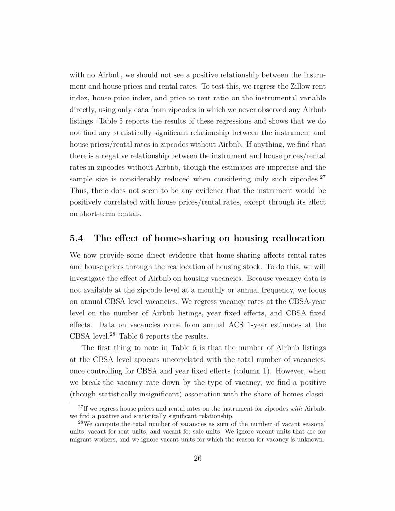
with no Airbnb, we should not see a positive relationship between the instru-ment and house prices and rental rates. To test this, we regress the Zillow rentindex, house price index, and price-to-rent ratio on the instrumental variabledirectly, using only data from zipcodes in which we never observed any Airbnblistings. Table 5 reports the results of these regressions and shows that we donot find any statistically significant relationship between the instrument andhouse prices/rental rates in zipcodes without Airbnb. If anything, we find thatthere is a negative relationship between the instrument and house prices/rentalrates in zipcodes without Airbnb, though the estimates are imprecise and thesample size is considerably reduced when considering only such zipcodes.27

Thus, there does not seem to be any evidence that the instrument would bepositively correlated with house prices/rental rates, except through its effecton short-term rentals.

5.4 The effect of home-sharing on housing reallocation

We now provide some direct evidence that home-sharing affects rental ratesand house prices through the reallocation of housing stock. To do this, we willinvestigate the effect of Airbnb on housing vacancies. Because vacancy data isnot available at the zipcode level at a monthly or annual frequency, we focuson annual CBSA level vacancies. We regress vacancy rates at the CBSA-yearlevel on the number of Airbnb listings, year fixed effects, and CBSA fixedeffects. Data on vacancies come from annual ACS 1-year estimates at theCBSA level.28 Table 6 reports the results.

The first thing to note in Table 6 is that the number of Airbnb listingsat the CBSA level appears uncorrelated with the total number of vacancies,once controlling for CBSA and year fixed effects (column 1). However, whenwe break the vacancy rate down by the type of vacancy, we find a positive(though statistically insignificant) association with the share of homes classi-

27If we regress house prices and rental rates on the instrument for zipcodes with Airbnb,we find a positive and statistically significant relationship.

28We compute the total number of vacancies as sum of the number of vacant seasonalunits, vacant-for-rent units, and vacant-for-sale units. We ignore vacant units that are formigrant workers, and we ignore vacant units for which the reason for vacancy is unknown.

26

fied as vacant for seasonal or recreational use and a negative (and statisticallysignificant) association with the share of homes that are vacant-for-rent andvacant-for-sale.

It is important to note that the Census Bureau classifies homes as vacanteven if they are temporarily occupied by persons who usually live elsewhere.Thus, homes allocated permanently to the short-term market are supposed tobe classified as vacant, and will likely also be classified as seasonal or recre-ational homes by their owners and/or neighbors.29 The positive association ofAirbnb with vacant-seasonal homes, and the negative association with vacant-for-rent and vacant-for-sale homes is therefore consistent with absentee land-lords substituting away from the rental and for-sale markets for long-termresidents and allocating instead to the short-term market.

6 Conclusion

Our results suggest that Airbnb growth can explain 0.27% in annual rentgrowth and 0.49% in annual house price growth from 2012 to 2016. Theincreases to rental rates and house prices occur through two channels. In thefirst channel, home-sharing increases rental rates by inducing some landlords toswitch from supplying the market for long-term rentals to supplying the marketfor short-term rentals. The increase in rental rates through this channel is thencapitalized into house prices. In the second channel, home-sharing increaseshouse prices directly by enabling homeowners to generate income from excesshousing capacity. This raises the value of owning relative to renting, andtherefore increases the price-to-rent ratio directly.

Our paper contributes to the debate surrounding home-sharing policy.Critics of home-sharing argue that it raises housing costs for local residents,and we find evidence confirming this effect. On the other hand, we also findevidence that home-sharing increases the value of homes by allowing owners tobetter utilize excess capacity. In our view, regulations on home-sharing should

29When a home is vacant, Census workers will interview neighbors about the occupancycharacteristics of the home.

27

(at most) seek to limit the reallocation of housing stock from the long-termto the short-term markets, without discouraging the use of home-sharing byowner-occupiers. One regulatory approach could be to only levy occupancytax on home sharers who rent the entire home for an extended period of time,or to require a proof of owner-occupancy in order to avoid paying occupancytax.

To summarize the state of the literature on home-sharing, researchers havefound that home-sharing 1) raises local rental rates by causing a reallocationof the housing stock; 2) raises house prices through both the capitalization ofrents and the increased ability to use excess capacity; and 3) induces marketentry by small suppliers of short-term housing who compete with traditionalsuppliers (Zervas et al. (2017)). More research is needed, however, in orderto achieve a more complete welfare analysis of home-sharing. For example,home-sharing may have positive spillover effects on local businesses if it drivesa net increase in tourism demand. On the other hand, home-sharing mayhave negative spillover effects if tourists create negative amenities, such asnoise or congestion, for local residents. Moreover, home-sharing introducesan interesting new mechanism for scaling down the local housing supply inresponse to negative demand shocks—a mechanism that was not possible whenall of the residential housing stock was allocated to the long-term market.

References

Chen, M. Keith, Judith A. Chevalier, Peter E. Rossi, and EmilyOehlsen, “The Value of Flexible Work: Evidence from Uber Drivers,”NBER Working Paper 23296, 2017.

Edelman, Benjamin G and Michael Luca, “Digital discrimination: Thecase of airbnb.com,” Harvard Business School Working Paper, 2014.

Edelman, Benjamin, Michael Luca, and Dan Svirsky, “Racial discrimi-nation in the sharing economy: Evidence from a field experiment,” AmericanEconomic Journal: Applied Economics, 2017, 9 (2), 1–22.

28

Einav, Liran, Chiara Farronato, and Jonathan Levin, “Peer-to-PeerMarkets,” Annual Review of Economics, October 2016, 8, 615–635.

Fradkin, Andrey, “Search frictions and the design of online marketplaces,”Working Paper, Massachusetts Institute of Technology, 2015.

Gong, Jing, Brad N. Greenwood, and Yiping Song, “Uber Might BuyMe a Mercedez Benz: An Empirical Investigation of the Sharing Economyand Durable Goods Purchase,” SSRN Working Paper, 2017.

Hall, Jonathan V. and Alan B. Krueger, “An Analysis of the LaborMarket for Uber’s Driver-Partners in the United States,” ILR Review, 2017.

Horna, Keren and Mark Merantea, “Is Home Sharing Driving Up Rents?Evidence from Airbnb in Boston,” Journal of Housing Economics, 2017.

Horton, John J. and Richard J. Zeckhauser, “Owning, Using and Rent-ing: Some Simple Economics of the “Sharing Economy”,” NBER WorkingPaper 22029, 2016.

Lee, Dayne, “How Airbnb Short-Term Rentals Exacerbate Los Angeles’sAffordable Housing Crisis: Analysis and Policy Recommendations,” HarvardLaw & Policy Review, 2016, pp. 229–254.

Poterba, James M., “Tax Subsidies to Owner-Occupied Housing: An Asset-Market Approach,” The Quarterly Journal of Economics, 1984, 99 (4), 729–752.

Zervas, Georgios, Davide Proserpio, and John W. Byers, “The Riseof the Sharing Economy: Estimating the Impact of Airbnb on the HotelIndustry,” Journal of Marketing Research, 2017, 54 (5), 687–705.

29

Figure 1: Google Trends Search Index for Airbnb (Worldwide, 2008-2017)0

2040

6080

100

Goo

gle

Tren

ds In

dex

2008 2010 2012 2014 2016 2018Date

Note: Weekly Google Trends index for the single English search term “Airbnb”,from any searches worldwide. Google Trends data are normalized so that thedate with the highest search volume is given the value of 100.

30

Figure 2: Map of Airbnb Listings by Zipcode, 2011-2016

Note: The number of listings is calculated using method 1 in Table 1. Loglistings is set to zero if there are zero listings. Geographic areas withoutzipcode boundary information are colored white.

31

Figure 3: Total Number of Airbnb Listings (US, 2008-2016)0

500

1000

Tota

l # A

irbnb

Lis

tings

(1,0

00s)

2008 2010 2012 2014 2016 2018Date

Note: The number of listings is calculated using method 1 in Table 1.

32

Figure 4: Trends in Zillow Home Value Index by “Tourstiness” of Zipcode

9010

011

012

013

0In

dex

(Jan

.201

1=10

0)

2008 2010 2012 2014 2016 2018Date

1 2 3 4Quartile for # of Food & Accommodations Establishments in 2010

ZHVI

9899

100

101

102

Inde

x (J

an.2

011=

100)

2008 2010 2012 2014 2016 2018Date

1 2 3 4Quartile for # of Food & Accommodations Establishments in 2010

ZHVI (residuals)

Note: The top panel plots the ZHVI index, normalized to January 2011=100, av-eraged within different groups of zipcodes based on their level of “touristiness” in2010. Touristiness is measured as the number of establishments in the food servicesand accommodations sector (NAICS code 72) in 2010, and the zipcodes are sepa-rated into four equally sized groups. The bottom panel plots the residuals from aregression of the ZHVI on zipcode fixed effects and CBSA-month fixed effects.

33

Table 2: Size of Airbnb Relative to the Housing Stock (zipcodes, 100 largestCBSAs)

p10 p20 p50 p75 p90Year 2011

Airbnb Listings 0.00 0.00 0.00 1.83 7.50Housing Unites 1,058.00 2,812.50 7,438.00 12,829.00 18,037.00Airbnb as a Percentage ofTotal Housing Units 0.00 0.00 0.00 0.02 0.10Renter-occupied Unites 0.00 0.00 0.001 0.09 0.39Vacant Units 0.00 0.00 0.01 0.26 1.02Vacant-for-rent Units 0.00 0.00 0.13 1.30 5.58

Year 2015Airbnb Listings 0.58 2 7.92 28.50 98.90Housing Unites 1,089.00 2,894.50 7,582.00 13,128.00 18,282.00Airbnb as a Percentage ofTotal Housing Units 0.01 0.05 0.13 0.40 1.37Renter-occupied Unites 0.05 0.18 0.54 1.66 5.26Vacant Units 0.13 0.52 1.60 4.76 14.00Vacant-for-rent Units 0.67 2.45 8.26 27.00 89.00

Note: This table reports the size of Airbnb relative to the housing stock, by zipcodesfor the 100 largest CBSAs as measured by 2010 population. The number of Airbnblistings is calculated using method 1 in Table 1. Data on housing stocks, occupancycharacteristics, and vacancies come from ACS zipcode level 5-year estimates. Wereport data for the year 2015 instead of 2016 because data from the 2016 ACS arenot yet available.

34

Table 3: The Effect of Airbnb on Rental Rates and House Prices

Panel A Panel B Panel CDep var: ln Rent Index Dep var: ln Price Index Dep var: ln Price/Rent

(1) (2) (3) (4) (1) (2) (3) (4) (1) (2) (3) (4)ln Airbnb Listings 0.0843*** 0.00622*** 0.0442*** 0.0421*** 0.157*** 0.00702*** 0.0788*** 0.0761*** 0.0737*** 0.000749 0.0309*** 0.0312***

(0.00213) (0.000522) (0.00326) (0.00324) (0.00382) (0.000749) (0.00621) (0.00619) (0.00184) (0.000775) (0.00442) (0.00451)ln Median HH Income 0.0261*** 0.0152 -0.0205

(0.00850) (0.0140) (0.0137)ln Population 0.0363*** 0.0680*** 0.0284**

(0.00901) (0.0152) (0.0141)College Share 0.0656*** 0.0696** 0.00887

(0.0195) (0.0297) (0.0283)Employment Rate 0.0461** 0.0323 -0.00930

(0.0204) (0.0341) (0.0311)Zipcode FE Yes Yes Yes Yes Yes Yes Yes Yes YesCBSA-year-month FE Yes Yes Yes Yes Yes Yes Yes Yes YesInstrumental variable Yes Yes Yes Yes Yes YesObservations 592,439 592,439 592,439 592,007 525,241 525,241 525,241 524,972 496,663 496,648 496,648 496,451R2 0.128 0.991 0.990 0.990 0.153 0.996 0.994 0.994 0.142 0.979 0.978 0.978Significance levels: *** p<0.01, ** p<0.05, * p<0.1

Note: The number of Airbnb listings is calculated using method 1 in Table 1. To avoid taking the log of a zero, one is added to thenumber of Airbnb listings before taking logs. Because zipcode demographic characteristics are not available at the monthly (or evenannual level), zipcode-month measures for household income, population, college share, and employment rate are interpolated fromthe 2011 and 2015 ACS 5-year estimates. Clustered standard errors at the zipcode level are reported in parenthesis.

35

Table 4: The Effect of Airbnb on Rental Rates and House Prices, by Owner-Occupancy Rate

Panel A Panel B Panel CDep var: ln Rent Index Dep var: ln Price Index Dep var: ln Price/Rent

(1) (2) (3) (4) (1) (2) (3) (4) (1) (2) (3) (4)ln Airbnb Listings 0.189*** 0.0198*** 0.0505*** 0.0483*** 0.356*** 0.0293*** 0.0737*** 0.0698*** 0.173*** 0.00762*** 0.0207*** 0.0196***

(0.00622) (0.00129) (0.00319) (0.00321) (0.0116) (0.00202) (0.00491) (0.00491) (0.00583) (0.00181) (0.00377) (0.00384)... × Owner-Occupancy Rate -0.111*** -0.0223*** -0.0357*** -0.0336*** -0.217*** -0.0357*** -0.0492*** -0.0453*** -0.114*** -0.0108*** -0.0106** -0.00968**

(0.0102) (0.00178) (0.00364) (0.00362) (0.0182) (0.00279) (0.00567) (0.00561) (0.00884) (0.00248) (0.00425) (0.00426)ln Median HH Income 0.0113 0.00463 -0.0139

(0.00926) (0.0144) (0.0148)ln Population 0.0588*** 0.121*** 0.0665***

(0.00907) (0.0155) (0.0153)College Share 0.0694*** 0.0798*** 0.0197

(0.0211) (0.0293) (0.0307)Employment Rate 0.0681*** 0.119*** 0.0511

(0.0217) (0.0347) (0.0339)Zipcode FE Yes Yes Yes Yes Yes Yes Yes Yes YesCBSA-year-month FE Yes Yes Yes Yes Yes Yes Yes Yes YesInstrumental Variable Yes Yes Yes Yes Yes YesObservations 492,119 492,119 492,119 491,759 437,691 437,691 437,691 437,470 412,565 412,550 412,550 412,389R2 0.223 0.992 0.991 0.991 0.251 0.997 0.996 0.997 0.227 0.982 0.981 0.981Significance levels: *** p<0.01, ** p<0.05, * p<0.1

Note: The number of Airbnb listings is calculated using method 1 in Table 1. To avoid taking the log of a zero, one is added to thenumber of Airbnb listings before taking logs. Because zipcode demographic characteristics are not available at the monthly (or evenannual level), zipcode-month measures for household income, population, college share, and employment rate are interpolated fromthe 2011 and 2015 ACS 5-year estimates. The owner-occupancy rate is calculated as the number of owner-occupied housing unitsdivided by the sum of owner-occupied units and renter-occupied units, using ACS 5-year estimates. Clustered standard errors at thezipcode level are reported in parenthesis.

36

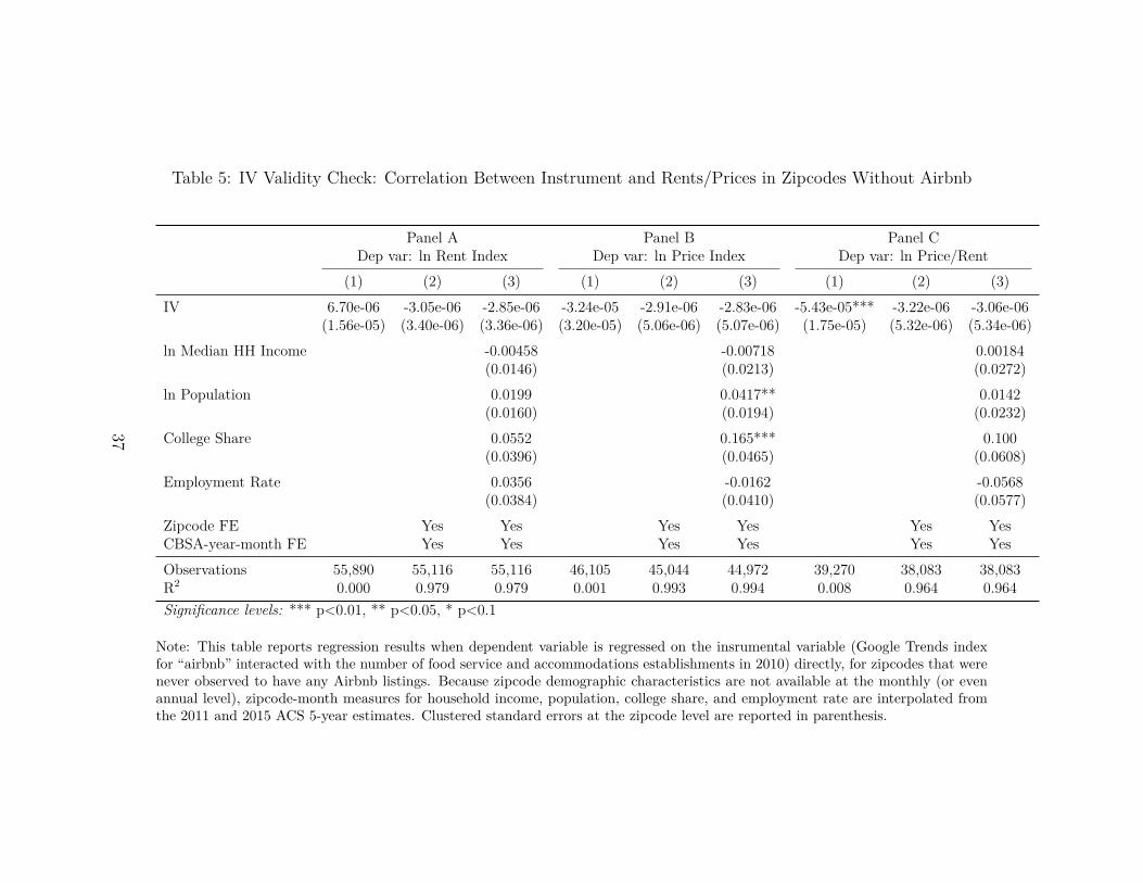
Table 5: IV Validity Check: Correlation Between Instrument and Rents/Prices in Zipcodes Without Airbnb

Panel A Panel B Panel CDep var: ln Rent Index Dep var: ln Price Index Dep var: ln Price/Rent

(1) (2) (3) (1) (2) (3) (1) (2) (3)IV 6.70e-06 -3.05e-06 -2.85e-06 -3.24e-05 -2.91e-06 -2.83e-06 -5.43e-05*** -3.22e-06 -3.06e-06

(1.56e-05) (3.40e-06) (3.36e-06) (3.20e-05) (5.06e-06) (5.07e-06) (1.75e-05) (5.32e-06) (5.34e-06)ln Median HH Income -0.00458 -0.00718 0.00184

(0.0146) (0.0213) (0.0272)ln Population 0.0199 0.0417** 0.0142

(0.0160) (0.0194) (0.0232)College Share 0.0552 0.165*** 0.100

(0.0396) (0.0465) (0.0608)Employment Rate 0.0356 -0.0162 -0.0568

(0.0384) (0.0410) (0.0577)Zipcode FE Yes Yes Yes Yes Yes YesCBSA-year-month FE Yes Yes Yes Yes Yes YesObservations 55,890 55,116 55,116 46,105 45,044 44,972 39,270 38,083 38,083R2 0.000 0.979 0.979 0.001 0.993 0.994 0.008 0.964 0.964Significance levels: *** p<0.01, ** p<0.05, * p<0.1

Note: This table reports regression results when dependent variable is regressed on the insrumental variable (Google Trends indexfor “airbnb” interacted with the number of food service and accommodations establishments in 2010) directly, for zipcodes that werenever observed to have any Airbnb listings. Because zipcode demographic characteristics are not available at the monthly (or evenannual level), zipcode-month measures for household income, population, college share, and employment rate are interpolated fromthe 2011 and 2015 ACS 5-year estimates. Clustered standard errors at the zipcode level are reported in parenthesis.

37

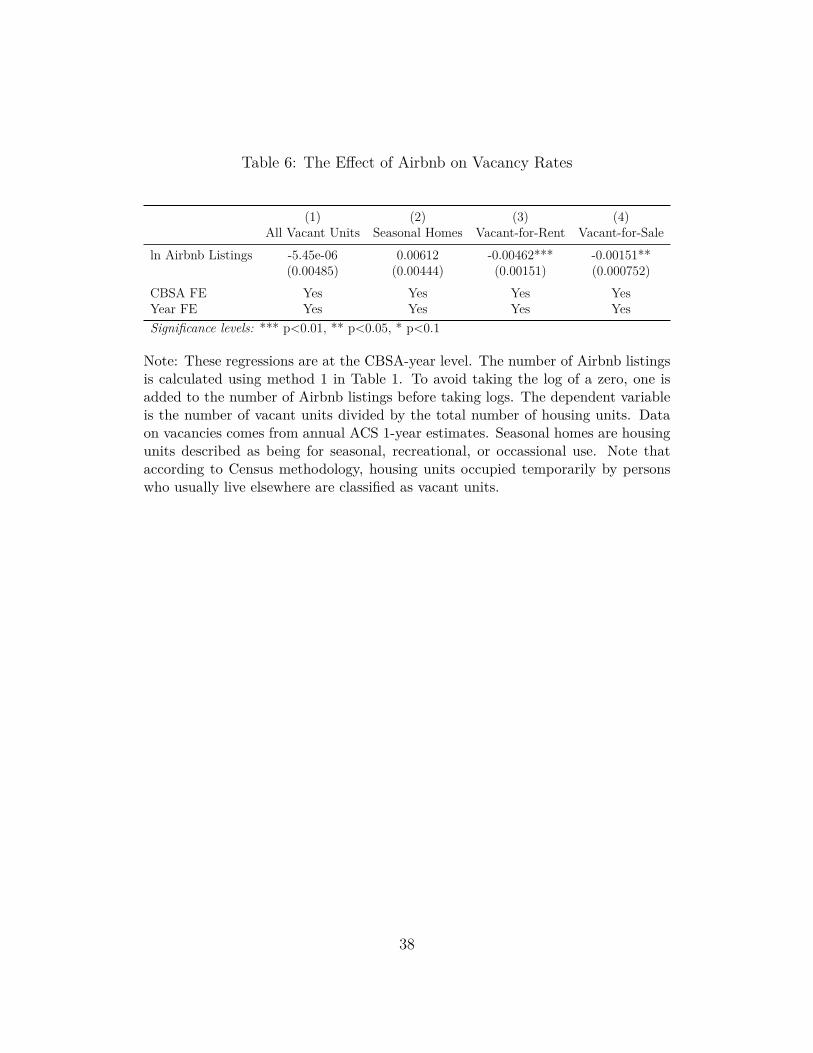
Table 6: The Effect of Airbnb on Vacancy Rates

(1) (2) (3) (4)All Vacant Units Seasonal Homes Vacant-for-Rent Vacant-for-Sale

ln Airbnb Listings -5.45e-06 0.00612 -0.00462*** -0.00151**(0.00485) (0.00444) (0.00151) (0.000752)

CBSA FE Yes Yes Yes YesYear FE Yes Yes Yes YesSignificance levels: *** p<0.01, ** p<0.05, * p<0.1

Note: These regressions are at the CBSA-year level. The number of Airbnb listingsis calculated using method 1 in Table 1. To avoid taking the log of a zero, one isadded to the number of Airbnb listings before taking logs. The dependent variableis the number of vacant units divided by the total number of housing units. Dataon vacancies comes from annual ACS 1-year estimates. Seasonal homes are housingunits described as being for seasonal, recreational, or occassional use. Note thataccording to Census methodology, housing units occupied temporarily by personswho usually live elsewhere are classified as vacant units.

38

For Online Publication: Appendix

A Model with Endogenous Owner-Occupiers

The model in Section 2 can be extended to allow the share of owner-occupiersto be endogenous. However, ex-ante heterogeneity in potential buyers needs tobe introduced or else an equilibrium with all three of renters, owner-occupiers,and absentee landlords would require that equations (4) and (10) both beequal. If they were not, then either long-term residents will outbid absenteelandlords to own all the housing, or the opposite will happen.

We introduce heterogeneity in the most parsimonious way possible. Con-sider a set of N individuals who potentially interact with a local housingmarket. Each individual can choose to be a renter, an owner-occupier, an ab-sentee landlord, or none of the above. Let us normalize the utility for “none ofthe above” to zero. The present value of utility that person i gets from beinga renter is:

ui,r = U − 11− δR + εi,r

= ur + εi,r

Here, U is the present value of amenities that the individual gets from beinga resident in this market. 1

1−δR is the present value of rents. εi,r is an idiosyn-cratic utility shock which is known ex-ante. The present value that person igets from being an owner is:

ui,o = U − P + 11− δγg(Q− c) + εi,o

= uo + εi,o

Here, U is again the present value of amenities, P is the purchase price ofhousing, and 1

1−δγg(Q − c) is the present value of rents received from sellingexcess capacity on the peer-to-peer market. Finally, the present value that

39

person i gets from being an absentee landlord is:

ui,a = −P + 11− δ [R + g(Q−R− c)] + εi,a

= ua + εi,a

For analytical tractability, let the utility shocks εi be distributed i.i.d. type 1extreme value. The share of individuals that choose option j out of j = {r, o, a}is:

sj = expuj1 +∑

k∈{r,o,a} expukThe equilibrium conditions determining R and P are:

(sa + so)N = H

and:[1− f(Q−R− c)] saN = srN

The first condition is the market clearing condition for the housing market asa whole; i.e. the number of absentee landlords plus owner-occupiers is equal tothe housing stock. The second condition is the market clearing condition forthe long-term rental market; i.e. the number of renters is equal to the numberof absentee landlords allocating housing to the long-term market.

We leave the derivation of analytical results for this model to future workor enterprising students. For this Appendix, we will simply present somenumerical results which are consistent with all the key predictions in Section2. Choosing N = 10, H = 2, U = $500, 000, δ = 0.95, γ = 0.1, Q = $25, 000,and letting the distribution of idiosyncratic costs to listing in the short-termmarket be uniform from $0 to $100,000, we consider a change of c from ∞(no home-sharing) to c = 0 (costless home-sharing). Table 7 below shows theresults. Consistent with the model, the introduction of home-sharing underthese model parameters results in a modest increase in both rental rates andhouse prices, and the increase in house prices is larger than the increase inrental rate. The qualitative results are robust to different parameter choices.

40

Table 7: Simulation Results

c =∞ c = $50k ∆Rent $25,069 $25,193 0.49%Price $502,773 $507,702 0.98%

B Comparison to Insideairbnb.com Data

To validate the accuracy of our dataset, in this section we compare our Airbnblisting information with that obtained by Insideairbnb.com, a website thatkeeps track of Airbnb data in a few key cities. Data from Insideairbnb havebeen featured in USA Today and have been used for policy research by thecity of San Francisco. Because Insideairbnb.com does not collect data all overthe U.S., but rather for a handful of specific cities, we compare data for thecity of Los Angeles. The Insideairbnb scrape of Los Angeles with timestampJuly 3, 2016 contains 15,958 listings. Out of 15,958 listings, we are able toexacly match 15,768 listings, or approximately 99% of the Insideairbnb.comlistings (our snapshot data contains a total of 15,808 listings for the city of LosAngeles for the month of June 2016—the closest period to the Insidearibnb.comdata). Results are similar when comparing to Insideairbnb data for other cities.Due to the high degree of match between our data and Insideairbnb, we arereassured of the accuracy of our data.

C Robustness Checks

In this section, we show that our main results are robust to the alternativemethods of calculating Airbnb supply, as discussed in Section 3. Table 8 repli-cates the full specification as in Table 4, with zipcode demographic controls,using the methods for calculating Airbnb supply listed in Table 1. Columns(1), (2), and (3) of each panel in Table 8 correspond to methods 2, 3, and4 of Table 1, respectively. The results when using methods 2 and 3 are very

41

similar in magnitude to the results using method 1. The results when usingmethod 4 are somewhat different, but we note that this is primarily driven byan imprecise estimate of the effect of Airbnb on rents. Otherwise, the resultsare qualitatively similar.

In Table 9, we show that our results are robust to the choice of CBSAsto include in our estimation sample. The main results used the 100 largestCBSAs, but Table 9 shows that the results are not particularly sensitive tothis choice.

42

Table 8: Robustness Checks: Alternative Methods of Measuring Airbnb Supply

Panel A Panel B Panel CDep var: ln Rent Index Dep var: ln Price Index Dep var: ln Price/Rent

(1) (2) (3) (1) (2) (3) (1) (2) (3)ln Airbnb Listings 0.0472*** 0.0496*** -0.00634 0.0678*** 0.0716*** 0.119*** 0.0179*** 0.0193*** 0.135***

(0.00335) (0.00351) (0.0141) (0.00521) (0.00545) (0.0234) (0.00371) (0.00389) (0.0303)... × Owner-Occupancy Rate -0.0318*** -0.0352*** -0.0210* -0.0422*** -0.0474*** -0.131*** -0.00773 -0.00945* -0.108***

(0.00440) (0.00440) (0.0118) (0.00684) (0.00684) (0.0195) (0.00521) (0.00505) (0.0255)ln Median HH Income 0.00622 0.00851 0.105*** -0.00236 8.13e-05 0.0126 -0.0164 -0.0155 -0.0887

(0.00923) (0.00925) (0.0386) (0.0144) (0.0144) (0.0442) (0.0148) (0.0148) (0.0594)ln Population 0.0625*** 0.0612*** -0.0239 0.127*** 0.125*** -0.124*** 0.0694*** 0.0686*** -0.142**

(0.00894) (0.00902) (0.0407) (0.0157) (0.0157) (0.0460) (0.0153) (0.0153) (0.0563)College Share 0.0637*** 0.0661*** 0.0121 0.0713** 0.0737** 0.0553 0.0178 0.0184 0.0723

(0.0206) (0.0207) (0.0812) (0.0292) (0.0292) (0.0815) (0.0307) (0.0307) (0.113)Employment Rate 0.0694*** 0.0688*** 0.0950 0.116*** 0.117*** -0.0957 0.0512 0.0512 -0.268*

(0.0213) (0.0215) (0.0926) (0.0343) (0.0345) (0.0995) (0.0337) (0.0337) (0.142)Method for Calculating # Listings 2 3 4 2 3 4 2 3 4Zipcode FE Yes Yes Yes Yes Yes Yes Yes Yes YesCBSA-year-month FE Yes Yes Yes Yes Yes Yes Yes Yes YesInstrumental Variable Yes Yes Yes Yes Yes Yes Yes Yes YesObservations 491,759 491,759 77,868 437,470 437,470 69,099 412,389 412,389 66,781R2 0.991 0.991 0.998 0.996 0.996 0.999 0.981 0.981 0.994Significance levels: *** p<0.01, ** p<0.05, * p<0.1

Note: Columns (1), (2), and (3) calculate Airbnb listings according to methods 2, 3 and 4 of Table 1, respectively. To avoid taking the log of a zero,one is added to the number of Airbnb listings before taking logs. Because zipcode demographic characteristics are not available at the monthly (or evenannual level), zipcode-month measures for household income, population, college share, and employment rate are interpolated from the 2011 and 2015 ACS5-year estimates. The owner- occupancy rate is calculated as the number of owner-occupied housing units divided by the sum of owner-occupied units andrenter-occupied units, using ACS 5-year estimates. Standard errors are clustered at the zipcode level.

43

44

Table 9: Robustness Checks: Alternative Samples of CBSAs

Panel A Panel B Panel CDep var: ln Rent Index Dep var: ln Price Index Dep var: ln Price/Rent

(1) (2) (3) (1) (2) (3) (1) (2) (3)ln Airbnb Listings 0.0527*** 0.0483*** 0.0457*** 0.0781*** 0.0698*** 0.0646*** 0.0232*** 0.0196*** 0.0182***

(0.00376) (0.00321) (0.00298) (0.00570) (0.00491) (0.00452) (0.00437) (0.00384) (0.00357)... × Owner-Occupancy Rate -0.0353*** -0.0336*** -0.0319*** -0.0483*** -0.0453*** -0.0434*** -0.0105** -0.00968** -0.00969**

(0.00397) (0.00362) (0.00349) (0.00611) (0.00561) (0.00539) (0.00459) (0.00426) (0.00413)ln Median HH Income 0.0156 0.0113 0.00886 0.0257 0.00463 0.00758 0.00170 -0.0139 -0.00897

(0.0107) (0.00926) (0.00863) (0.0170) (0.0144) (0.0131) (0.0161) (0.0148) (0.0137)ln Population 0.0449*** 0.0588*** 0.0608*** 0.113*** 0.121*** 0.112*** 0.0797*** 0.0665*** 0.0588***

(0.0105) (0.00907) (0.00858) (0.0187) (0.0155) (0.0140) (0.0177) (0.0153) (0.0141)College Share 0.0640*** 0.0694*** 0.0711*** 0.0629* 0.0798*** 0.0754*** 0.0211 0.0197 0.00775

(0.0248) (0.0211) (0.0195) (0.0352) (0.0293) (0.0268) (0.0354) (0.0307) (0.0285)Employment Rate 0.0750*** 0.0681*** 0.0672*** 0.117*** 0.119*** 0.102*** 0.0418 0.0511 0.0400

(0.0256) (0.0217) (0.0201) (0.0409) (0.0347) (0.0308) (0.0379) (0.0339) (0.0308)Sample: N largest CBSAs 50 150 200 50 150 200 50 150 200Zipcode FE Yes Yes Yes Yes Yes Yes Yes Yes YesCBSA-year-month FE Yes Yes Yes Yes Yes Yes Yes Yes YesInstrumental Variable Yes Yes Yes Yes Yes Yes Yes Yes YesObservations 388,780 491,759 547,202 351,285 437,470 491,466 332,705 412,389 459,122R2 0.991 0.991 0.991 0.996 0.997 0.997 0.982 0.981 0.981Significance levels: *** p<0.01, ** p<0.05, * p<0.1

Note: The samples in columns (1), (2), and (3) are the 50, 150, and 200 largest CBSAs, respectively (the baseline was 100 CBSAs as reported in Table4. The number of Airbnb listings is calculated using method 1 in Table 1. To avoid taking the log of a zero, one is added to the number of Airbnblistings before taking logs. Because zipcode demographic characteristics are not available at the monthly (or even annual level), zipcode-month measures forhousehold income, population, college share, and employment rate are interpolated from the 2011 and 2015 ACS 5-year estimates. The owner-occupancyrate is calculated as the number of owner-occupied housing units divided by the sum of owner-occupied units and renter-occupied units, using ACS 5-yearestimates. Standard errors are clustered at the zipcode level.

45