thesis approved major advisor dean
TRANSCRIPT
Thesis Approved
Major Advisor
Dean
/THERMAL COEFFICIENTS AND THEIR
RELATION TO THE ONSAGER COEFFICIENTS
BY
CHUNGTE W. CHEN'/
A THESIS
Submitted to the Faculty of the Graduate School of the Creighton University in Partial Fulfillment of the
Requirements for the Degree of Master of Science in the Department of Physics.
Omaha, 1976
V
ACKNOWLEDGEMENTS
The author wishes to express his thanks and sincere apprecia
tion to the members of the Department of Physics of the Creighton
University especially Dr. Robert E. Kennedy whose many hours of
consultation and advice made this work possible.
The author also would like to express his gratitude to
Dr. Thomas Zepf for many helpful discussions, and Fr. Thomas
McShane for assistance in computer work.
This work is dedicated to the author's wife, Jenna, and his
parents, whose encouragement and help have been invaluable.

TABLE OF CONTENTS
Chapter Page
I Introduction ...................................... 1
II Unifying Principle in Physics:VariationalPrinciple ...................................... 7
(a) M e c h a n i c s ................................. 7(b) Electromagnetic Theory ..................... 8(c) Optics .................................... 10(d) Thermodynamics ........................... 15
III The Coefficients of Onsager's Equations ......... 22
IV Electric Conductivity ............................ 28
(a) Bardeen's Method ......................... 30(b) Our Method to Derive the Relaxation
Time .................................. 35
V Thermal Conductivity .............................. 39
(a) The Formula of the ThermalConductivity ......................... 40
(b) Callaway's Model ......................... 43(c) Klemens' Model ......................... 44(d) Our M o d e l .................................. 45(e) The Result of Our M o d e l .................... 46
VI Thermopower .........................................
VII Conclusion......................................... 60
vi
BIBLIOGRAPHY 65
vii
LIST OF ILLUSTRATIONS
Figure Page
2.1 A Lagrangian diagram for two different regions . . . . 12
2.2 The ray diagram from one region to another............... 14
5.1 Thermal conductivity of Ge................................. 49
6.1 The graph of first order thermopower...................... 56
6.2 Fermi surfaces and their change in area withincreasing energy...................................... 59
SECTION I
Introduction
Nonequilibrium thermodynamics is a phenomenological theory of
matter, which describes the behavior of a system due to differences
within the system or between the system and its surroundings. These
differences give rise to thermodynamic forces which can cause flows of
quantities such as charge and energy. One example of such a force is
the temperature gradient due to a temperature difference across the
ends of a solid. The flow caused by this force is energy flow or
heat current.
When two or more thermodynamic forces are applied on a system,
they can interfere with each other, and give rise to new effects.
Although many thermodynamic physicist, such as Rauss, Peltier, and
Seebeck, discovered some important phenomena about these new effects,
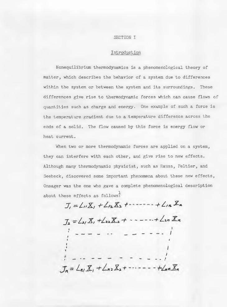
Onsager was the one who gave a complete phenomenological description
about these effects as follows!
J, =■ Z//X/ - h + + /-/n. %-*-
Jx - Lx/ -2T/ -+ ----- +Z**
— L-m 2 -X* _
Page 2
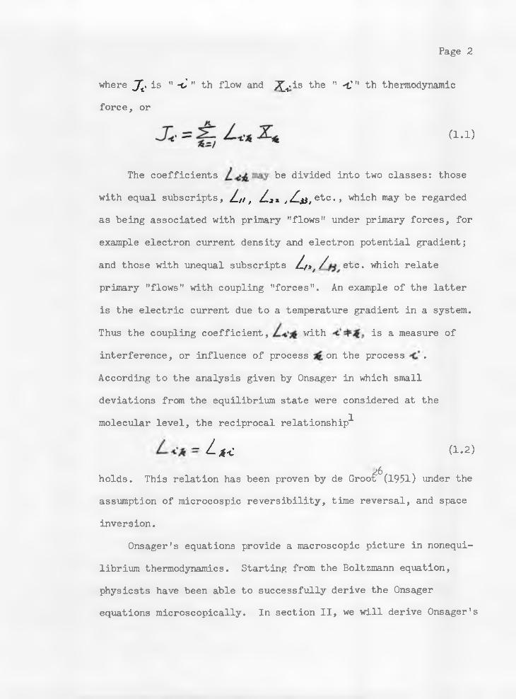
where J~t. is " ~C " th flow and ^^.is the " 'C" th thermodynamic
force, or
(1.1)
The coefficients be divided into two classes: those
with equal subscripts, An, Aax , Z ^ e t c . , which may be regarded as being associated with primary "flows" under primary forces, for
example electron current density and electron potential gradient;
and those with unequal subscripts A/xJ / etc. which relate
primary "flows" with coupling "forces". An example of the latter
is the electric current due to a temperature gradient in a system.
Thus the coupling coefficient, with is a measure of
interference, or influence of process on the process .
According to the analysis given by Onsager in which small
deviations from the equilibrium state were considered at the
molecular level, the reciprocal relationship^-
— L (1 .2 )
holds. This relation has been proven by de Groo£^(1951) under the
assumption of microcospic reversibility, time reversal, and space
inversion.
Onsager1s equations provide a macroscopic picture in nonequi
librium thermodynamics. Starting from the Boltzmann equation,
physicsts have been able to successfully derive the Onsager
equations microscopically. In section II, we will derive Onsager1s

Page 3
equations by using the variational principle, a technique which has
been used in many other fields of physics, such as Classical Mechan-
In principle, we can measure the Onsager coefficients,
directly, but it is very complicated in practice. In section III,
certain of the Onsager coefficients, £-«>£, will be derived in terms
of thermal coefficients: electrical conductivity, thermal conductiv
ity, and thermoelectric power.
The electrical conductivity is governed by the scattering of
electrons by the lattice vibrations. The lattice vibration is gen
erally analyzed into a system of independent sound waves, which can
be interpreted as quasi-particles which possess momentum and energy.
analogy with the photons of electromagnetic waves. The interaction
between electrons and phonons can be characterized by the relaxation
by electrons between collisions with phonons. The relaxation time
probability that the electron will pass from state % to state &
2ics, Electromagnetism, Optics, and Quantum Mechanics.
These quanta of lattice vibrational
time r • This is often crudely interpreted as the mean time taken
T is associated with the transition rate the transition
(1.3)
where Jfl is the differential solid angle in space. Fermi's
golden rule number 2 provides the traditional way to calculate

Page 4
the transition rate. An alternate way to calculate the transition
rate is to use the equation of motion
f ] (1.4)
where f is density operator, and f-f is Hamiltonian operator. Using
this method the transition rate for a pure metal is calculated in
section IV. We get the same result as Bardeen^ The method we use
provides a more realistic physical picture.
Thermal Conductivity is calculated by considering that the3heat is carried by electrons and phonons. Although most of the
heat is transferred by electrons in a metal, thermal conduction in
semiconductors and insulators is mainly determined by phonon-phonon
interaction, phonon-boundary scattering and phonon-impurity scatt
ering^’ ^ Because the conservation of energy and momentum must be
satisfied, the two phonon stattering processes is impossible.3Although Pomeranchuk, in 1941, considered the four-phonon scatter
ing process in thermal conductivity, the thermal conduction is
dominated by three-phonon scattering processes. The relaxation
time due to phonon-phonon scattering, phonon-boundary scattering
and phonon-isotopic scattering is assumed in this thesis as follows
(see section V)
r-'= a*‘+ BJ*
22
(1.5)

Page 5
We not only can interpret the thermal conductivity at the low5temperature as Callaway's model, but also can explain the intermedi
ate temperature range. Ge has been used as a sample, and theg
result looks quite good when compared with the Geballe and Mull
experimental result.
To calculate the thermoelectric power we consider a conductor
heated at one end. Electrons at the hot end will, in general,
acquire increased energy relative to the cold end and will diffuse
to the cold end where their energy may be lowered. This is essent
ially the manner in which heat is conducted in a metal and is
accompanied by the accumlation of the negative charge at the cold
end, thus setting up an electric field between the ends of the
material. This electric field will build up until a state of
dynamic equilibrium is established between electrons urged down
the temperature gradient and electrostatic repulsion due to the ex
cess charge at the cold end. Then the number of electrons passing
through a cross section normal to the flow per second in each
direction will be equal, but the velocities of electrons proceed
ing from the hot end will be higher than those velocities of
electrons passing through the section from cold end. This differ
ence ensures that there is a continuous transfer of heat down the
temperature gradient without actual charge transfer once dynamic
equilibrium has been set up. This kind of phenomenon is called9the thermoelectric effect.

Page 6
The distribution function of the electrons , in the mater
ial can provide the information about the thermoelectric effect.
The general method to obtain the distribution function of electrons
h . is to solve the Boltzmann equation which involves a very3sophisticated integro-differential equation. In section VI, we use
a power series expansion to represent the distribution function
in terms of the electric field and the temperature gradient
instead of directly solving the Boltzmann equation. The result of
the first order approximation is exactly the same as that of the3 9traditionally used method.’ We also obtain the same expression
for the second order terms.
SECTION II
Unifying Principle in Physics - Variational Principle
The variational principle has been used to deal with the pro
blems in Mechanics, Optics, and Electromagnatism. In this section,
we will discuss briefly how this method is applied to classical
physics, then see how this method can be used to derive Onsager's
equations.
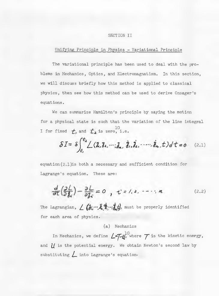
We can summarize Hamilton's principle by saying the motion
for a physical state is such that the variation of the line integral. ^ 10I for fixed £ and is zero, i.e.
S1= 5 Z a , (2.1)Jt,
equation (2.1 )is both a necessary and sufficient condition for
Lagrange's equation. These are:
= 0 <2-2)The Lagrangian, L ( k - . l f . - H must be properly identified
for each area of physics.
(a) Mechanics
In Mechanics, we define L - f# where ~J~ is the kinetic energy, and U is the potential energy. We obtain Newton's second law by
substituting l_ into Lagrange's equation*
Page 8
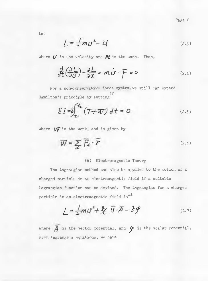
Let
L - -rwo1- u (2.3)
where {/ is the velocity and /Ki is the mass. Then,
& G k )- ik m,,lCr'F m0For a non-conservative force system,we still can extend
10Hamilton's principle by setting
(2.4)
S i (T tW )
where w is the work, and is given by
(2.5)
( 2 . 6 )
(b) Electromagnetic Theory
The Lagrangian method can also be applied to the motion of a
charged particle in an electromagnetic field if a suitable
Lagrangian function can be devised. The Lagrangian for a charged
particle in an electromagnetic field i s ^
J_ = % tr-fi-If (2.7>
where is the vector potential, and JJP is the scalar potential.
From Lagrange's equations, we have
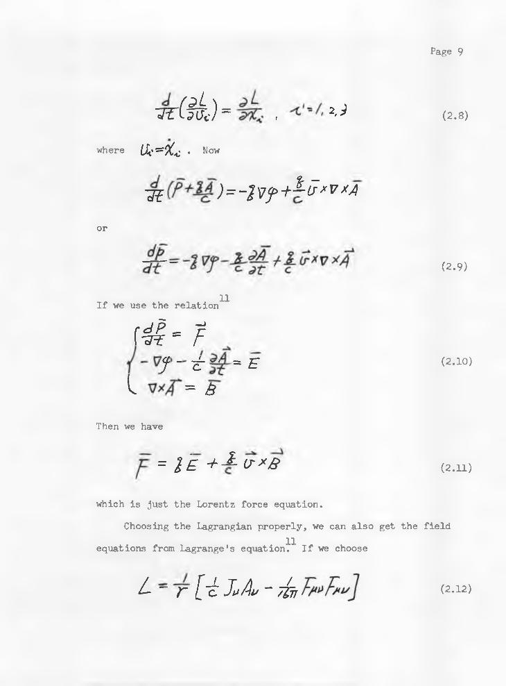
Page 9
Tr(fk)= ike . (2.8)
where Ue Cc • Now
1FE ) = - l V f - h ~ L r * v x A% ,7i
or
(2.9)
If we use the relation
& • ?{ - v f -
l = A
11
= B (2 . 10)
Then we have
f = l E +■*■<?>'& (2 . 11)
which is just the Lorentz force equation.
Choosing the Lagrangian properly, we can also get the field11equations from Lagrange's equation. If we choose
L- r{-k JpAv - yht (2 . 12)
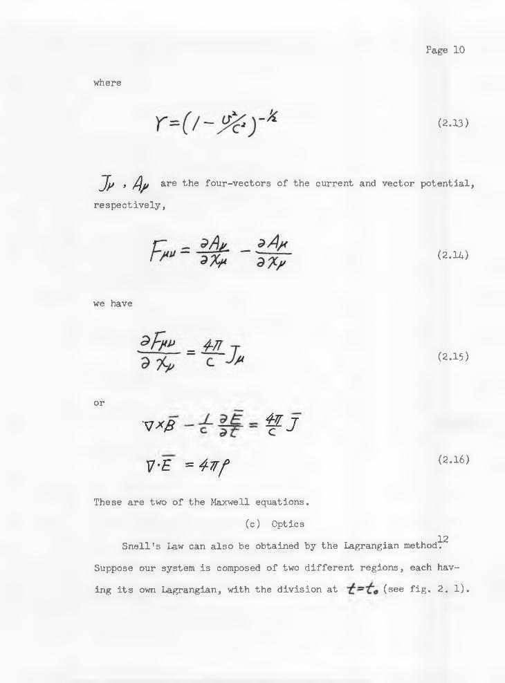
Page 10
where
(2.13)
Jy > Ay are the four-vectors of the current and vector potential,
respectively,
we have
(2. 14)
(2.15)
or
v*fi f J7-E =4rrf (2 . 16)
These are two of the Maxwell equations.
(c) Optics12Snell's Law can also be obtained by the Lagrangian method.
Suppose our system is composed of two different regions, each hav
ing its own Lagrangian, with the division at (see fig- 2. 1).
Page 11
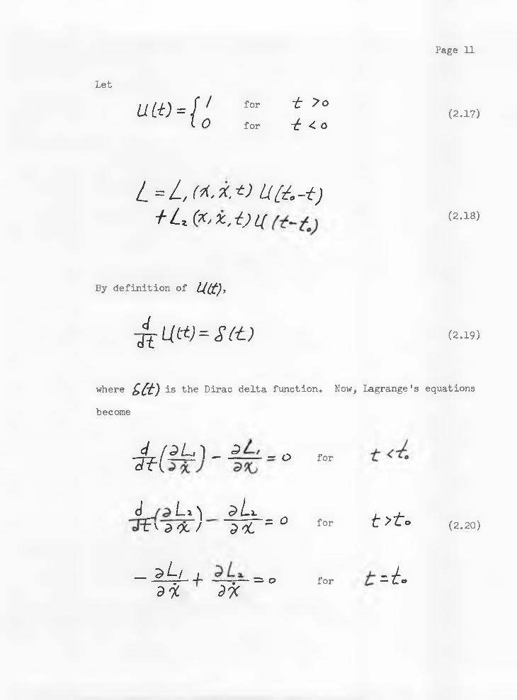
Let
Uit) = \ 'l 0for ~t 7 Ofor ~t <( O
1 = 1 , ( * . * . * ) U fa - * )+ L (x ,x , - t ) i(
By definition of UCt),
-kntt)=S(t)
(2.17)
(2.18)
(2.19)
where Ztt) is the Dirac delta function. Now, Lagrange's equations
become
d / Q L , - )~Z?i — ^ — O for
d L i F v a oc /
^ /-x2TC = ° for t> to (2.20)
- 3^-/ J. djc_--- i------- for
, ? x
li rV 0
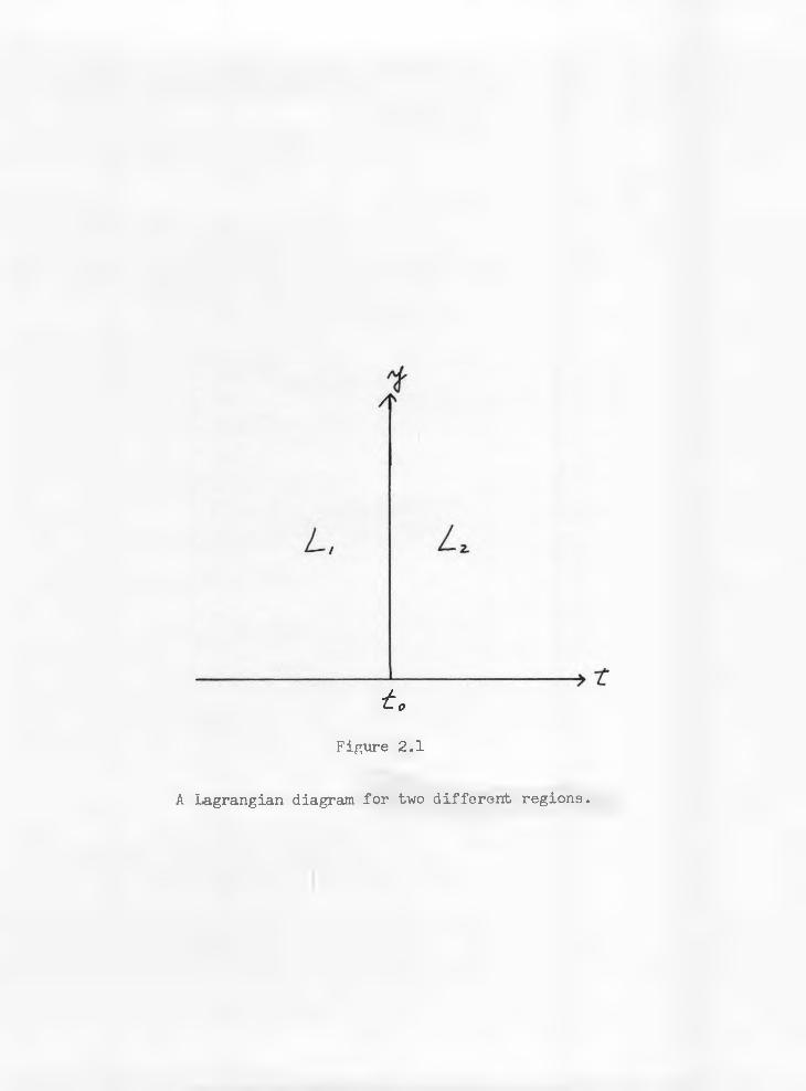
t.Figure 2.1
A Lagrangian diagram for two different regions.
Page 13
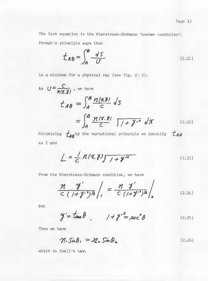
The last equation is the Wierstrass-Erdmann "corner condition".
Fermat's principle says that
(2. 21)
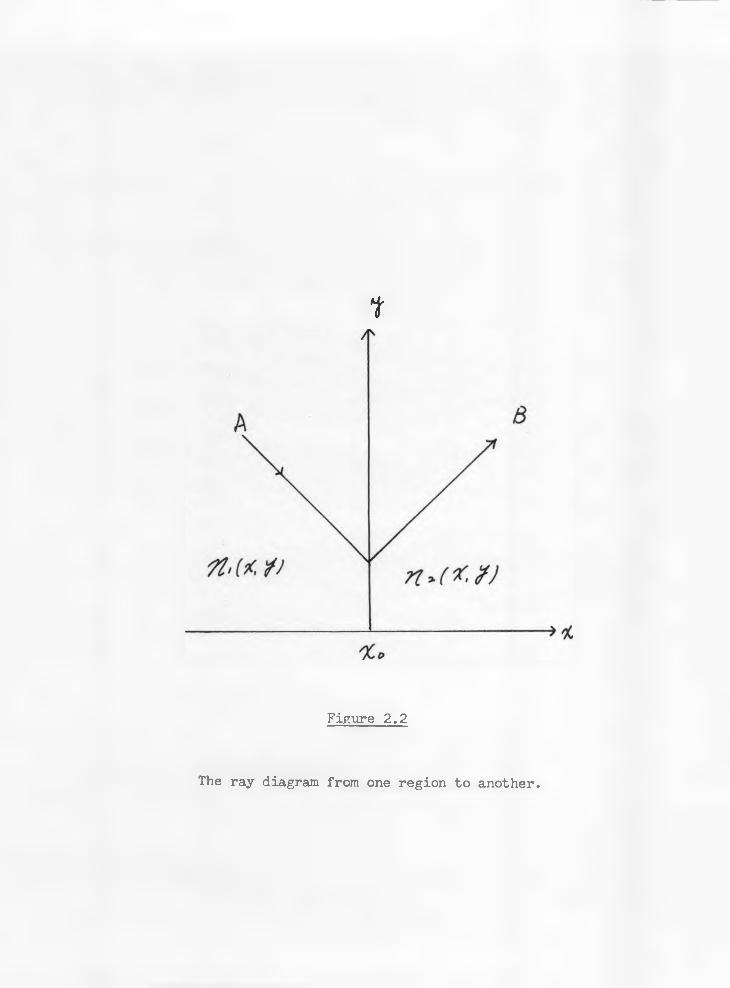
is a minimum for a physical ray (see fig. 2. 2).
_ cAs U" ~~ ZT7Z~iT\ > we haven(z,V
=£*£? n r r (2 . 22)
Minimizing the variational principle we identify t/93as I and
(2.23)
From the Wierstrass-Erdmann condition, we have
n f_/ /e. '( /+ ? ';» / / c 0+ T ')* U
But
y , /-/ f =/i£>c $Then we have
71'SmO' =
(2.24)
(2.25)
( 2 . 26 )
which is Snell's Law.
t
Figure 2.2
The ray diagram from one region to another.
Page 15
(d) Thermodynamics
As in parts (a), (b), and (c), we will identify the Lagrangian
such that Onsager's equations are the result of Hamilton's princi
ple. In nonequilibrium thermodynamics, the entropy is an increas
ing function of time, and the internal entropy is an extremum for
the steady-state case. If we define
(2.27)
where 3 is the entropy, and is the entropy production; then
when the system is in a steady-state. From the above dis
cussion, the Lagrangian can be defined as the entropy production
in steady-state nonequilibrium thermodynamics.
To obtain the Lagrangian, we try to point out the relation
between the Boltzmann equation and Onsager's equations'!'
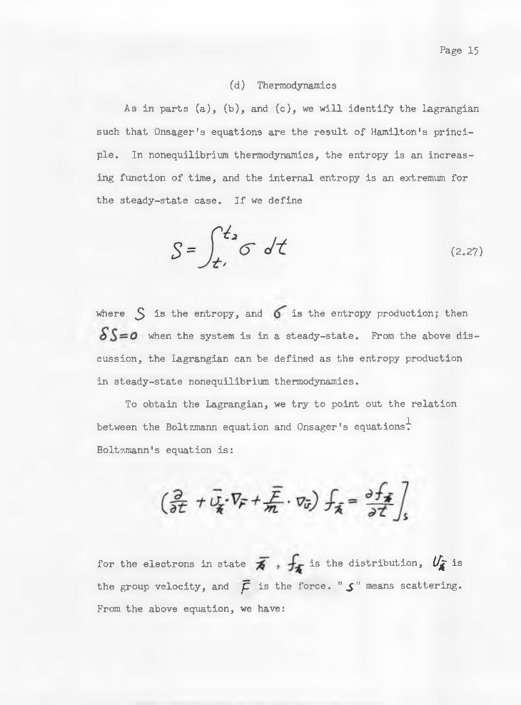
Boltzmann's equation is:
for the electrons in state is the distribution, L/jf isthe group velocity, and p is the force. " £'' means scattering.
From the above equation, we have:
Page 16
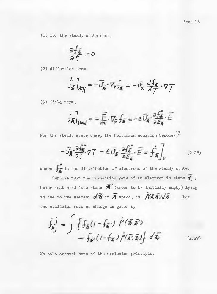
(1) for the steady state case,
= oa t(2) diffussion term,
£ 1 A # = = - U j t f y v T(3) field term,££
13
(2.28)
For the steady state case, the Boltzmann equation becomes:
- S> 1r v Twhere is the distribution of electrons of the steady state.
Suppose that the transition rate of an electron in state ^ ,
being scattered into state ^ (known to be initially empty) lying
in the volume element in /$ space, is . Then
the collision rate of change is given by£/= J(2.29)
We take account here of the exclusion principle.

Page 17
From microscopic reversibility, we have
f(i, V) = /VJ', P) (2 .30 )
Using a power series expansion for i_- , we haveA
Jh T& * * £ .
or
- /* $*/* ( ]X jHere is a measure of deviation of •£- from,^- , and
$% - 1'J -I
The Boltzmann equation can be rewritten as
- f s ’ & V T - Vg-**Sz£
where
3 J f *
= k j J (&■%-$$)p fa
(2.31)
(2.32)
(2.33)
(2.34)
From the law of conservation of energy, we have
(2.35)

Page 18
It provides:
P {* .* ') •p fc '.X )Equation (2.33) can be represented by the simple form:
j (h - ?$)
(2.36)
(2.37)
where J iv can be identified as the field term, and L h as
the scattering term. Multiplying equation(2,29) by i t and inte
grating with respect to , we obtain
KT
using equation (2.36), we can rewrite equation (2.38) as
tkf ff ( )*P6* *) J*'- - [ h i],«
(2 .38 )
(2.39)
Let us consider the statistical definition of entropy in a
Fermi-Dirac assembly:14
S* -k([frJLfg+0'k)M i'fx)]J* (2.40
Differentiating the above equation with respect to time, using
Page 19
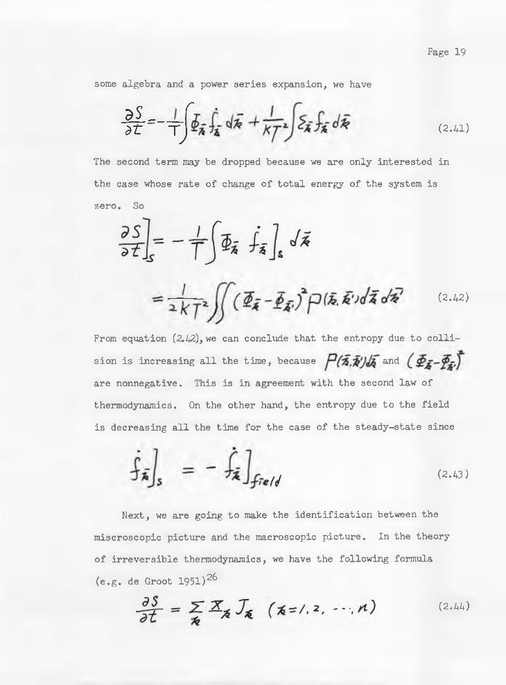
some algebra and a power series expansion, we have
S l atr
TJ (2.41)
The second term may be dropped because we are only interested in
the case whose rate of change of total energy of the system is
zero. So
(2 . 42)
From equation (2.42), we can conclude that the entropy due to colli
sion is increasing all the time, because and
are nonnegative. This is in agreement with the second law of
thermodynamics. On the other hand, the entropy due to the field
is decreasing all the time for the case of the steady-state since
/</ (2.43)
Next, we are going to make the identification between the
miscroscopic picture and the macroscopic picture. In the theory
of irreversible thermodynamics, we have the following formula
(e.g. de Groot 1951)^
(2.44)
Page 20
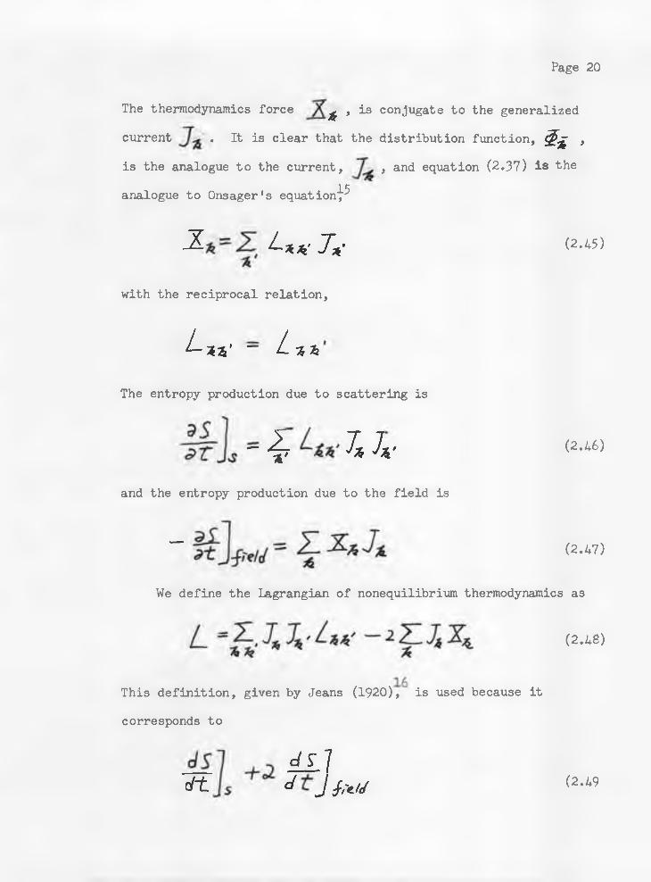
The thermodynamics force £ > is conjugate to the generalized current * It is clear that the distribution function, S i > is the analogue to the current, , and equation (2.37) is the
analogue to Onsager's equation"^
- 2 L+x J j
with the reciprocal relation,
(2.45)
L-**' - L %TkThe entropy production due to scattering is
~ ^ J*' (2,46)and the entropy production due to the field is
” (2.47)
We define the Lagrangian of nonequilibrium thermodynamics as
This definition, given by Jeans (1920), is used because it
corresponds to
(2.48)
d tdL1^ J //V</ (2.49
Page 21
which is, in the steady-state case, just the negative of the actual
entropy production in the dissipative process. Lagrange's equation
can now be written as
A - ( <? L )_ p Ld i ( s’jfc j (2-5o:
Substituting equation (2.48) into the above equation, we obtain
2-& -21s'Which is Onsager's equation.
(2.51)
SECTION III
The Coefficients of Onsager's Equations
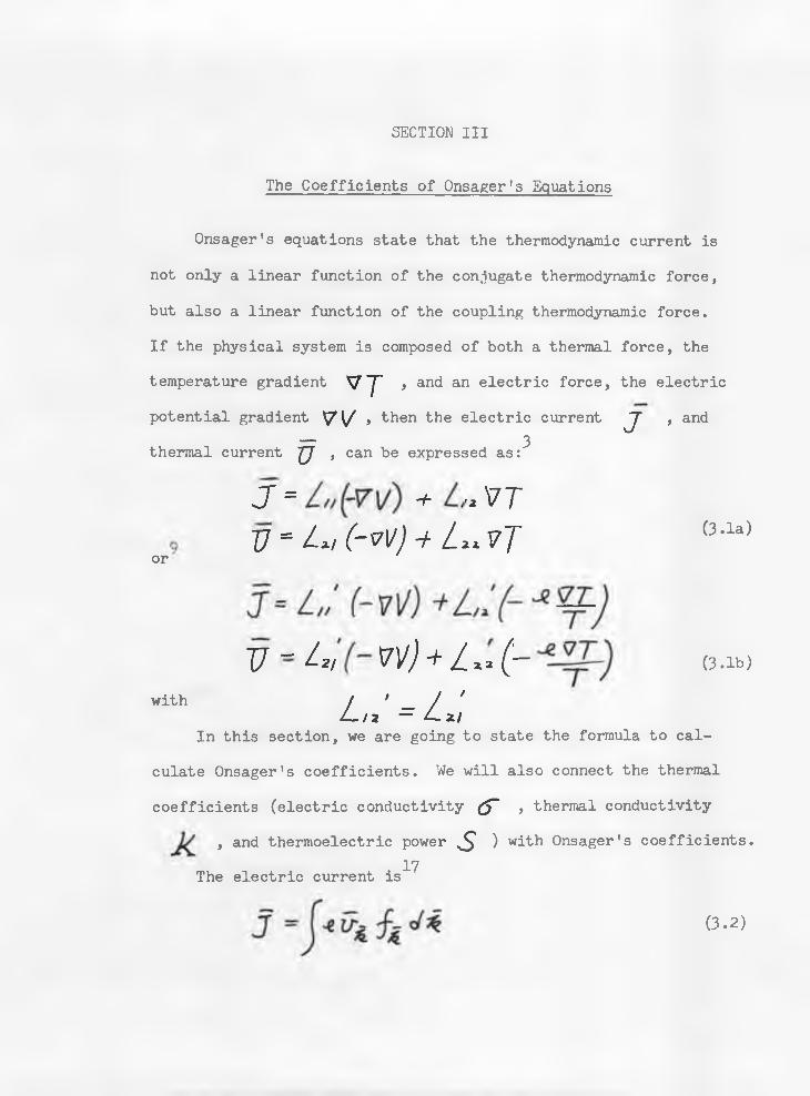
Onsager's equations state that the thermodynamic current is
not only a linear function of the conjugate thermodynamic force,
but also a linear function of the coupling thermodynamic force.
If the physical system is composed of both a thermal force, the
temperature gradient VT , and an electric force, the electric
potential gradient vv , then the electric current J~ , and— 3thermal current JJ , can be expressed as:
(3.1a)or
J = A,(-vv) + U V TV m L>, (-w ) + L * v T
V ~ 2/ VV) -+/_!*(— (3.1b)
with J ' _ / 'l—i 2 — ZLz/In this section, we are going to state the formula to cal
culate Onsager's coefficients. We will also connect the thermal
coefficients (electric conductivity (%* , thermal conductivity
, and thermoelectric power ^ ) with Onsager's coefficients.17The electric current is
(3.2)
Page 23
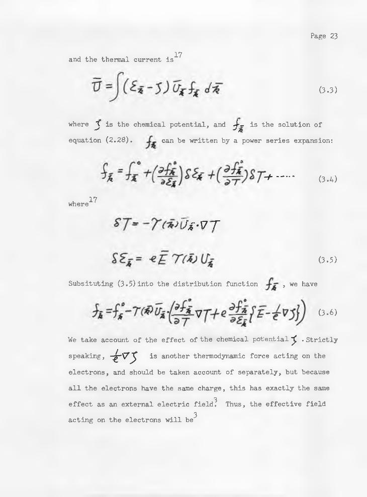
and the thermal current is17
(3.3)
where \ is the chemical potential, and 4 - is the solution of ^ J A,equation (2.28). can be written by a power series expansion:
- + ---- (3.4)
where17
-T w V g
(3.5)
(3.6)
Subsituting (3.5) into the distribution function , we have
We take account of the effect of the chemical potential^ .Strictly
speaking, -irvy is another thermodynamic force acting on the
electrons, and should be taken account of separately, but because
all the electrons have the same charge, this has exactly the same3effect as an external electric field. Thus, the effective field
3acting on the electrons will be
Page 24
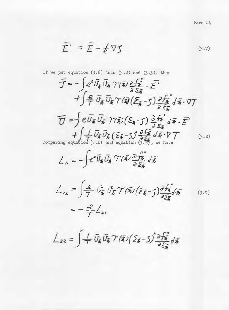
E‘ = E-<fIf we put equation (3.6) into (3.2) and (3.3), then
y = ' J V Ug (7* 7 Y * > | | l - f '
d £%y&)(£* -s) W-J* • r
* (£*-J/-IComparing equation (3.1) and equation (3*w, we have
3-fi
L„ = - T w d S - J j i
u -r
j M % </sT(*>fa-3)?g/*r= -^ZT
J 1 *<?£
(3.7)
(3.8)
(3.9)
Page 25
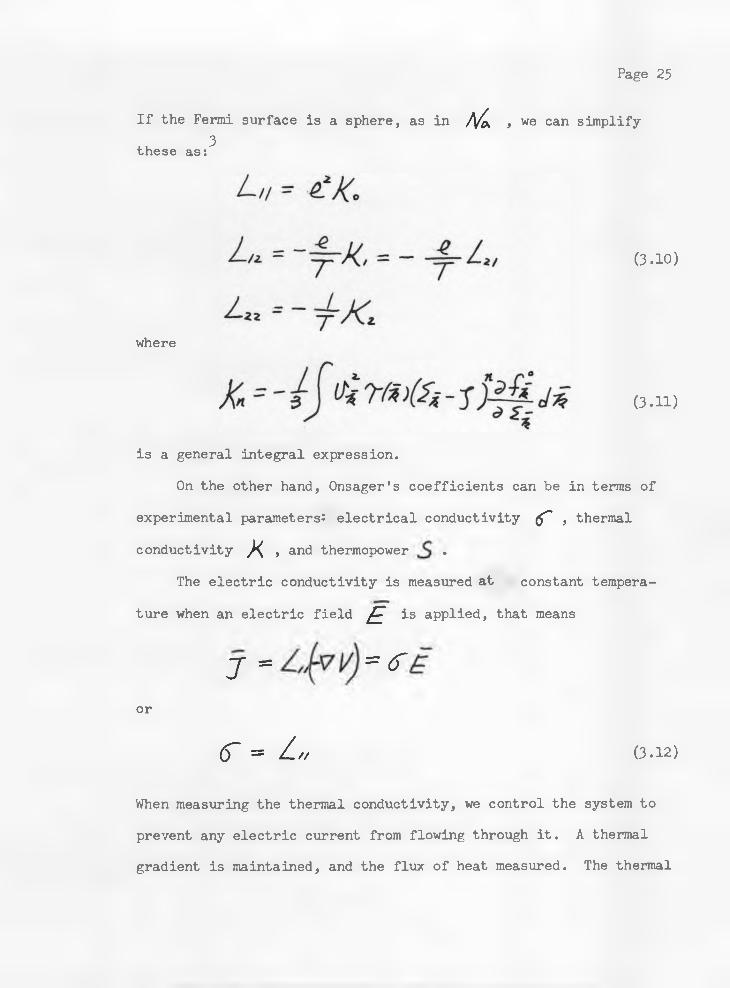
If the Fermi surface is a sphere, as in A/ck , we can simplify
these as:^
where
(3.10)
(3.11)
is a general integral expression.
On the other hand, Onsager's coefficients can be in terms of
experimental parameters: electrical conductivity <T , thermal
conductivity ^ , and thermopower .
The electric conductivity is measured at constant tempera
ture when an electric field £ is applied, that means
j = v)= <r ior
<r = L, (3.12)
When measuring the thermal conductivity, we control the system to
prevent any electric current from flowing through it. A thermal
gradient is maintained, and the flux of heat measured. The thermal
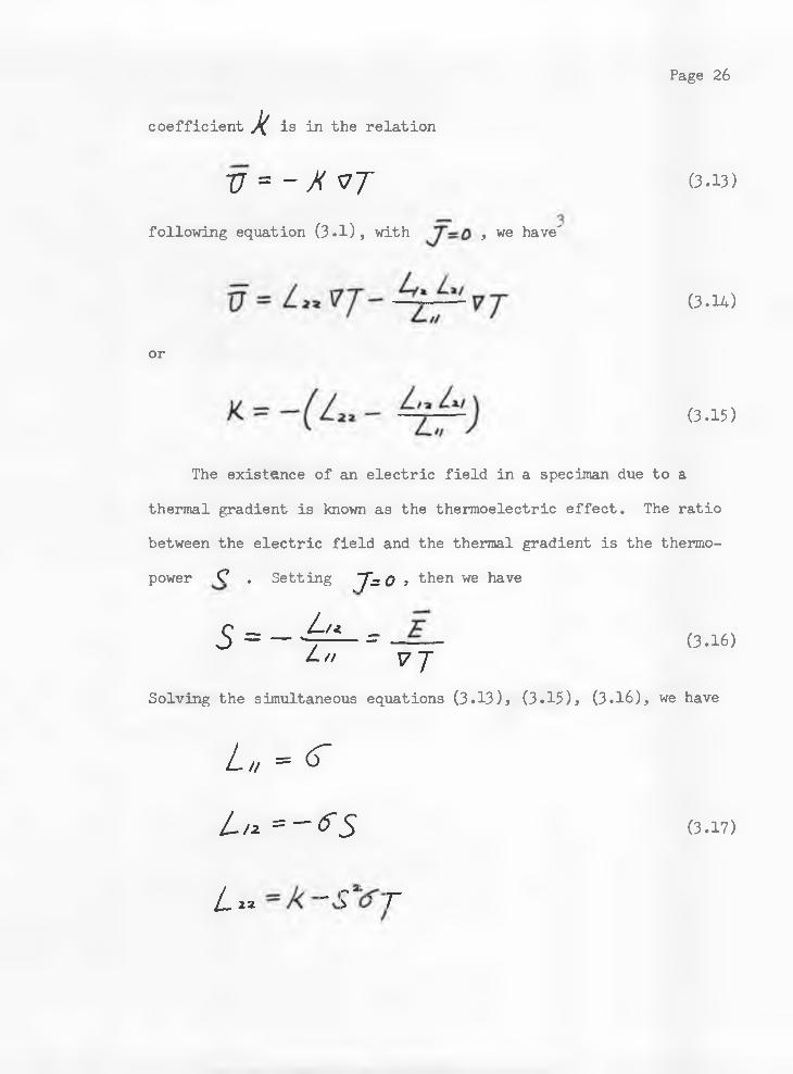
Page 26
kcoefficient X is in the relation
V = ~ k v jfollowing equation (3.1), with , we have"
(3.13)
(3.14)
or
(3.15)
The existence of an electric field in a speciman due to a
thermal gradient is known as the thermoelectric effect. The ratio
between the electric field and the thermal gradient is the thermo
power C . Setting 7=o , then we have
5 = - ^ = —Ln V j (3.16)
Solving the simultaneous equations (3.13), (3.15), (3.16), we have
La = <T Ln =-<T5Ln =k-s
(3.17)
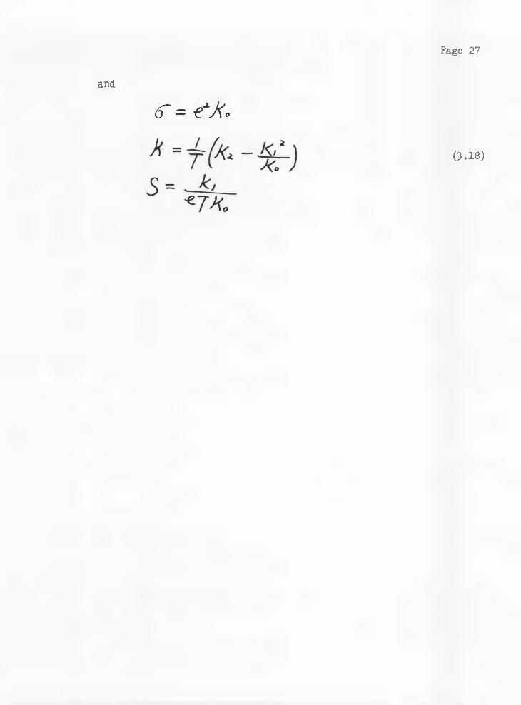
Page 27
and
<T = €J<.(3 .18)

SECTION IV
Electric Conductivity
In the previous section, we derived the Onsager coefficients
from the integral expression involving the relaxation time r •
On the other hand, the thermal coefficients, thermal conductivity,
electric conductivity, and thermal power, are also function of the
relaxation time. In this section, the relation between relaxation
time and transition rate derived by J. Bardeen^ will be discussed,
and then we will present a new way to determine the transition
rate.3, 17, 18The relaxation time / can be written as:
rr ( i '= \ ( / - n e e ) J-a (4.1)
where () is the angle between and , and (%>%') is the
transition rate of electrons from state to state due to the
thermal motion of the ions.
The thermal motion of the ions is generally analyzed into a
system of sound waves. The displacement of an ion at the lattice1point Kk is
+ 4 - / < , 4 > 4 )(4.2)
Page 29
in which ^ is the propagation vector, and 4 / is the angular
frequency of the wave. The index refers to three possi
ble directions of motion of ions.
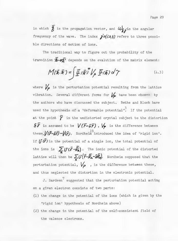
The traditional way to figure out the probability of the
transition depends on the evalution of the matrix element:
M (*>*)=f §<*) cJy/
(4.3)
where Yp is the perturbation potential resulting from the lattice
vibration. Several different forms for have been chosen by
the authors who have discussed the subject. Bethe and Bloch have3used the hypothesis of a "deformable potential". If the potential
at the point y~ in the undistorted crystal subject to the distortion
sr is assumed to be V(F-sr), Vr is the difference between
these, Nordheim^introduced the idea of "rigid ion".
If \f Lf) is the potential of a single ion, the total potential ofthe ions is The ionic potential of the distorted
lattice will then be 2l{J[y-Rh~&R*}- Nordheim supposed that the
perturbation potential, \/p , is the difference between these,
and thus neglected the distortion in the electronic potential.7J. Bardeen suggested that the perturbation potential acting
on a given electron consists of two parts:
(1 ) the change in the potential of the ions (which is given by the
"rigid ion" hypothesis of Nordheim above)
(2 ) the change in the potential of the self-consistent field of
the valence electrons.
Page 30
The second part tends to cancel the first. Let us consider the
transitions due to a single elastic wave of wave number ^ .
According to Bragg's diffraction law, the allowed transitions
are such that
- ± f + Kk ( ' * • ' * >
where kn is a vector of the reciprocal lattice space. Further
more, we require the conservation of energy:
“Jj (*•«>>
Using the "rigid ion" model and the concept of "self-consistent
field", we will discuss briefly first the method of deriving the
transition rate due to Bardeen, then use some of Bardeen's work to
present a new way to determine the transition rate.
(a) Bardeen's Method
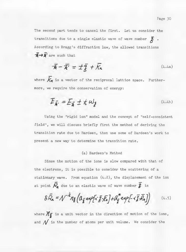
Since the motion of the ions is slow compared with that of
the electrons, it is possible to consider the scattering of a
stationary wave. From equation (4.2), the displacement of the ion
at point /?« due to an elastic wave of wave number £ is
sjz =a/ ' \ ( i “ 5 )
where is a unit vector in the direction of motion of the ions,
and V is the number of atoms per unit volume. We consider the
Page 31
scattering due to a single elastic wave of wave number , defined
by equation (4.5)above. The perturbation potential, , result
ing from this wave is the sum of two terms: , the change in
potential of the ions; and \Jp , the change in potential of the
self-consistent field of the valence electrons. Since the amplitude
of the vibration is small, it is possible to determine by a
perturbation procedure in which terms of higher order than the
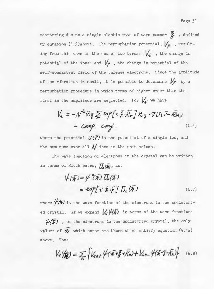
first in the amplitude are neglected. For [/£« we have
,4,Vi = - M & %g < 7 -a » ] y t f ■ m f -f . (U.b)
where the potential (/(f) is the potential of a single ion, and the sum rims over all ions in the unit volume.
The wave function of electrons in the crystal can be written
in terms of Bloch waves, as:
• %'?] Vote* (4.7)
where fa ) is the wave function of the electrons in the undistorted crystal. If we expand in terms of the wave functions
f(X) , of the electrons in the undistorted crystal, the only
values of •%' which enter are those which satisfy equation (4.4a) above. Thus,
(4.8)
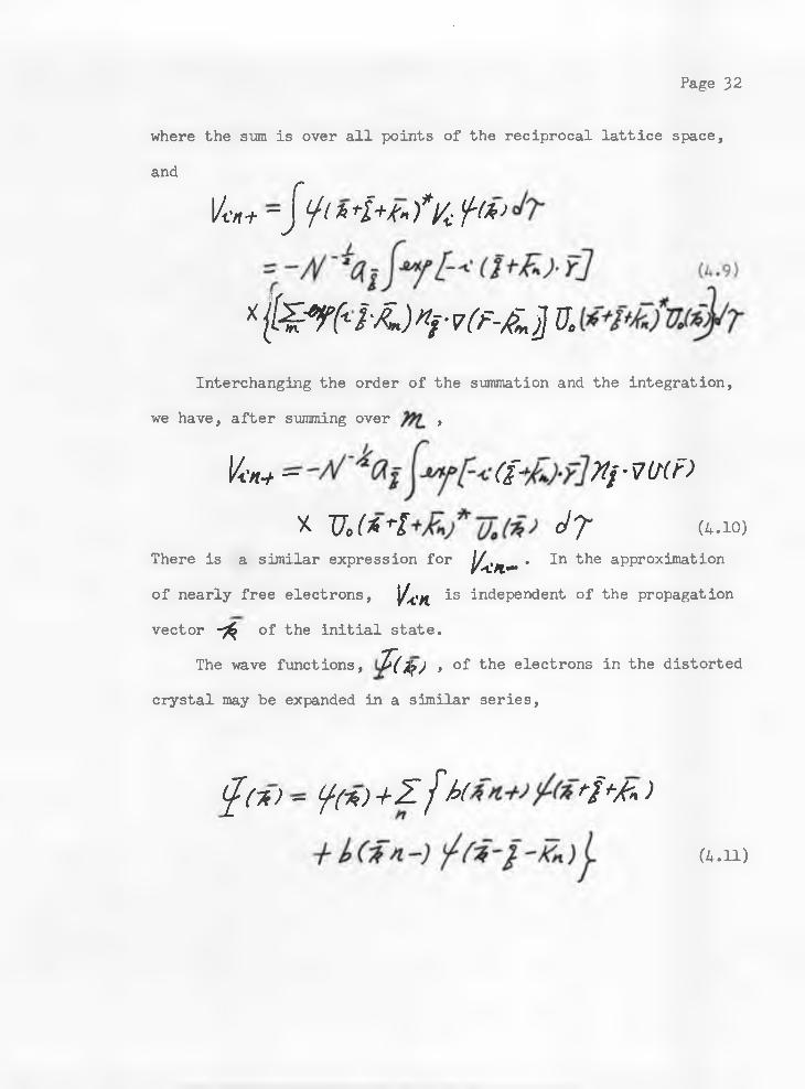
Page 32
where the sum is over all points of the reciprocal lattice space,
and
\f-cn-t ~ J f t k+l+k* fl/c ft*>
* (fe w • Mj *rv(f-& jj v.
Interchanging the order of the summation and the integration,
we have, after summing over ,
Vea+ - ( f m -Vl/(F)
x Vo(*rl c / T (4 .1 0 )There is a similar expression for K * - . In the approximation
of nearly free electrons, V<'n is independent of the propagation
vector -7^ of the initial state.
The wave functions, £(*> , of the electrons in the distorted
crystal may be expanded in a similar series,
(£ (*) - tf(ik) -h Z f k ( f f + A )
(4.11)

Page 33
The density of electrons is, to the first order,
f= Z ( )
= fo Uc l) (>s t A Jt f j 4 [U ih -n *-t
( f +&)•?!J (4 .1 2 )
where is the density of electrons in the undistorted crystal.
The summation over % is over all the occupied states. From
Poisson's equation
- * W € '( f - f ° ) (*.13)
we may determine the change is the electrostatic potential of the
electrons resulting from the distortion of the crystal, We make_ Athe further approximation that JJ0 £r/ , and solve the above
equation. To this approximation,
(4.14)
where
= 4*re / / (4.15)
Page 34
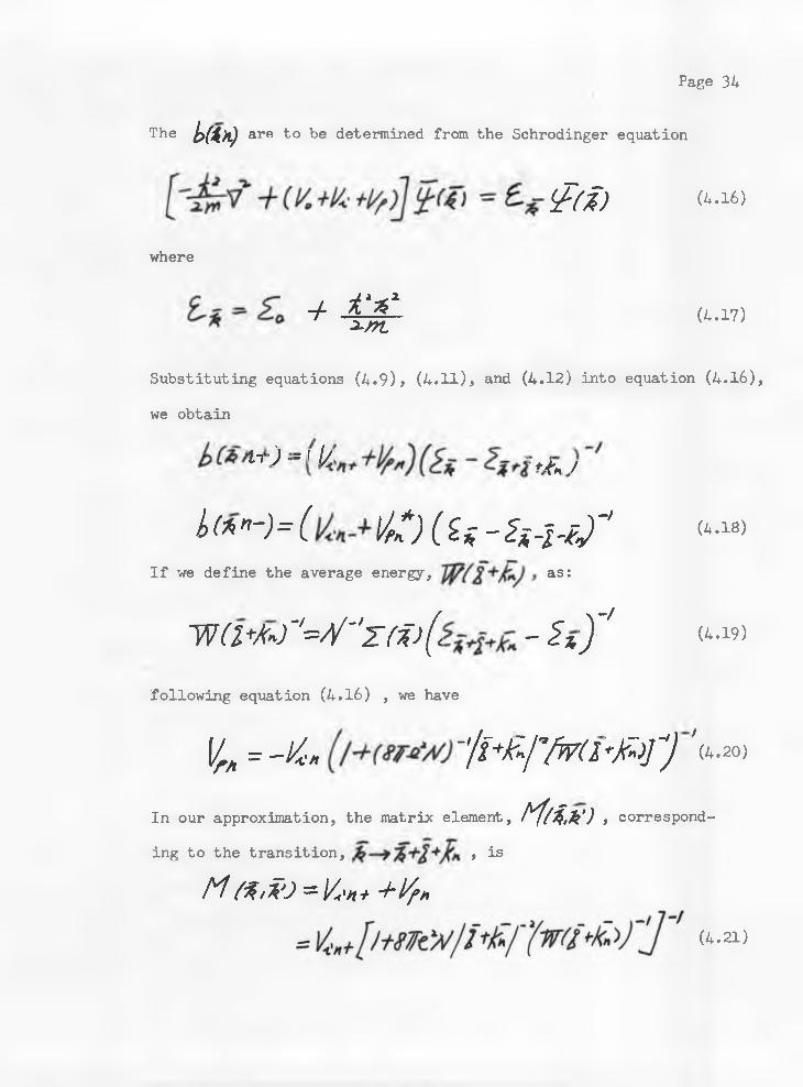
The b(4)t) are to be determined from the Schrodinger equation
<£(%) ('••16)
where
+ 4£- (4.17)
Substituting equations (4.9), (4.11), and (4.12) into equation (4.16),
we obtain
[>(bA+) ~ Z%rzt&)
l ( * " - ) = ( o ( u - h - l - f J " (4a8)If we define the average energy, as:
yva + M W ' r t f j ( - f*)"' (‘ -19)
following equation (4 .1 6 ) , we have
Vr/t = -k t* - j i * k ^ f w ( l ^ r ) V«»
In our approximation, the matrix element, l i / ix ) , correspond
ing to the transition, > isM f t ,%o=Vs>t+ +fy*
(4.21)
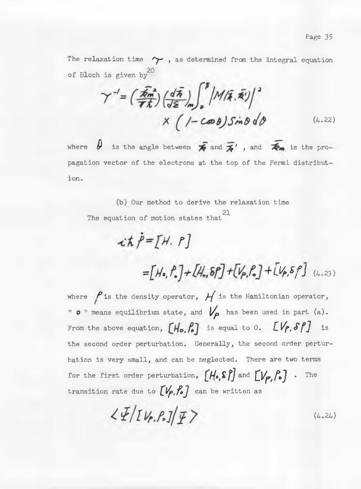
Page 35
The relaxation time rT , as determined from the integral equation
of Bloch is given by20
(4.22)
where $ is the angle between and ^ ; , and is the pro
pagation vector of the electrons at the top of the Fermi distribut
ion.
(b) Our method to derive the relaxation time21The equation of motion states that
r]=p/., t y f o t f ) +ft.23)
where Fis the density operator, }-( is the Hamiltonian operator," o " means equilibrium state, and \/p has been used in part (a).
From the above equation, is equal to 0. IV r.sf] is
the second order perturbation. Generally, the second order pertur
bation is very small, and can be neglected. There are two terms
for the first order perturbation, CH-sf] and D f / A J . The
transition rate due to 0W can be written as
(4.24)
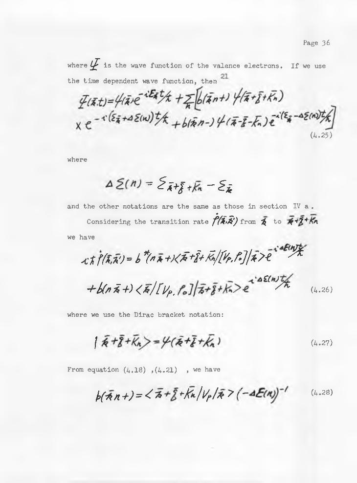
Page 36
where $ is the wave function of the valence electrons. If we use
the time dependent wave function, then
(4.25)
where
A 5- ( n)’ £ * > / - i iand the other notations are the same as those in section IV a .
•
Considering the transition rate f f i. i) from % to *+l+Kn we have
K t f ( t * ) =t % *+ ;< *+ 1+ & /& /•]!*> < y *
+ k fl a +) <*J[V?,, a }//* <'*-26>
where we use the Dirac bracket notation:
/ (4 .2 7 )
From equation (4.18) ,(4.21) , we have
\>(-*n+)=^~*> + l ' f o / V r / * 7(4.28)

Page 37
The Fermi distribution provides
(4.29)
Following (4.28) , (4.29) , equation (4.26) can be written as
Following the above equation, the transition rate from
other states due to should be written as:
to all
(4.31)

Page 38
The second term of the first order approximation that con
tributes to the transition rate is{jjiSfJ, where8f= £**>$(%) -
or
Sf- T(£n) +t>&+■ {!>(£a. -t )*-+1 (£n -)] (4.32)
where ^ is the Bloch function, and has been discussed in part
(a). Using the approximatI o n f’ wehave
(4.33)
From equation (4.31), (4.33), the total transition rate from
to any other state is
f •]- f f /<•*/]/r l - £ ) %x ~ £ $ )
(4.34)
The result of equation (4.31) for the total transition rate of22 23-state is exactly the same as the formula derived by Peierls 5
using the Fermi Golden rule II.

SECTION V
Thermal Conductivity
The thermal conductivity has been investigated for more than2fifty years. In 1929, Peierls pointed out that the thermal vibra
tions of the atoms in the solid can be resolved into normal modes,
and gave rise to the concept of phonons analogous to the photons
of radiation. The phonons obey Bose-Einstein statistics. The3equilibrium distribution function of phonons,/y , is
t r - - i fThe heat current is determined from the distribution of phonons,
which in turn is obtained as a solution of the Boltzmann equation.
In part (a), we will discuss the formula for the thermal conductivi-
ty.’ In part (b), we will discuss the Callaway model of relaxa
tion time for the thermal conductivity, and in part (c), we will7discuss the Klemens' model of the relaxation time for the high
temperature range. In part (d), we will present our model for the
relaxation time. Not only can we interpret the thermal conductivity
for the low temperature range, but we can also explain the inter
mediate temperature case. In part (e), we will show some computer
work for our model, and compare our result with the results predicted
from Callaway's model.
Page 40
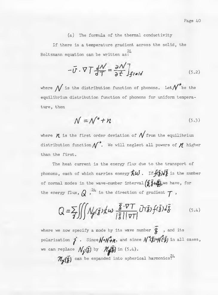
(a) The formula of the thermal conductivity
If there is a temperature gradient across the solid, the
Boltzmann equation can be written as:24
- t - v T 4 T - f r J U (5.2)
where j\J is the distribution function of phonons. Let/^ be the
equilibrium distribution function of phonons for uniform tempera
ture, then
Af -A/’ + (5.3)
where A is the first order deviation of f\f from the equilibrium distribution function A T- We will neglect all powers of /l higher
than the first.
The heat current is the energy flux due to the transport of
phonons, each of which carries energy iu). i is the number
of normal modes in the wave-number interval (U4) #we have, forp y
the energy flux, Q , in the direction of gradient ~J~ ,i'V T llM M Crrvft/Mt (5.o
where we now specify a mode by its wave number ^ , and its
polarization . S i n c e a n d since Hiim-h in all cases,
replace Afj$) by in (5.4).we can
can be expanded into spherical harmonics:?4

Page 41
(5.5)
where JA is the cosine of the angle between £ and gradient T - and the coefficient A / depends on j % j on^y* Substituting
equation(5.5)into equation(5.4) and integrating over all directions,
since
then
Q = £ | W +AfflW *•■•■]
using the orthogonality of the , we have
? )Thus only the first order in the expansion
the energy flux.
(5.6)
contributes to
24We now define a relaxation time y by'
- pA/ 1 _ p V 1_______ - / gdt ail Js y ~ y (5.7)
where
r/
T(*) (5.8)

Page 42
" C\ " represents the processes of the scattering. Substituting equation (5.8) into equation (5.7), and using equation (5.1), we
obtain
n (5.9)
Comparing equation (5.9) with equation (5.5), we have
a )
^ r * r (5-:Substituting equation (5.10) into equation (5.4), and dividing by
the temperature gradient, we have, for the thermal conductivity
of an isotropic solid,
Ji (5.11)
For simplicity, we assume that there is no difference between longi
tudinal and transverse phonons; then the number of modes in the
wave-number interval, elua-'- 1°gfpl% and2 - can be replaced by 3. So the thermal conductivity, , can
b^'written as:
2-1TU-k&/t'T'(f) * Ul- ^ JIQJ * T . f y C ^ r h l f
( 5 .12)
where we use the Debye model.In principle, we can calculate the thermal conductivity exactly
if we know the relaxation time. Lacking knowledge of crystal
Page 43
vibrational spectra and anharmonic forces in crystals, we can only
use a simple model of the relaxation time to calculate the thermal
conductivity. Although quite a few physicist have suggested
different models for the relaxation time, those models could not
explain the thermal conductivity over all the temperature ranges.
The most important models were suggested by Callaway'’ for low7temperature, and by P. G. Klemens1 for high temperature. We dis
cuss these two models briefly in part (b) and part (c).
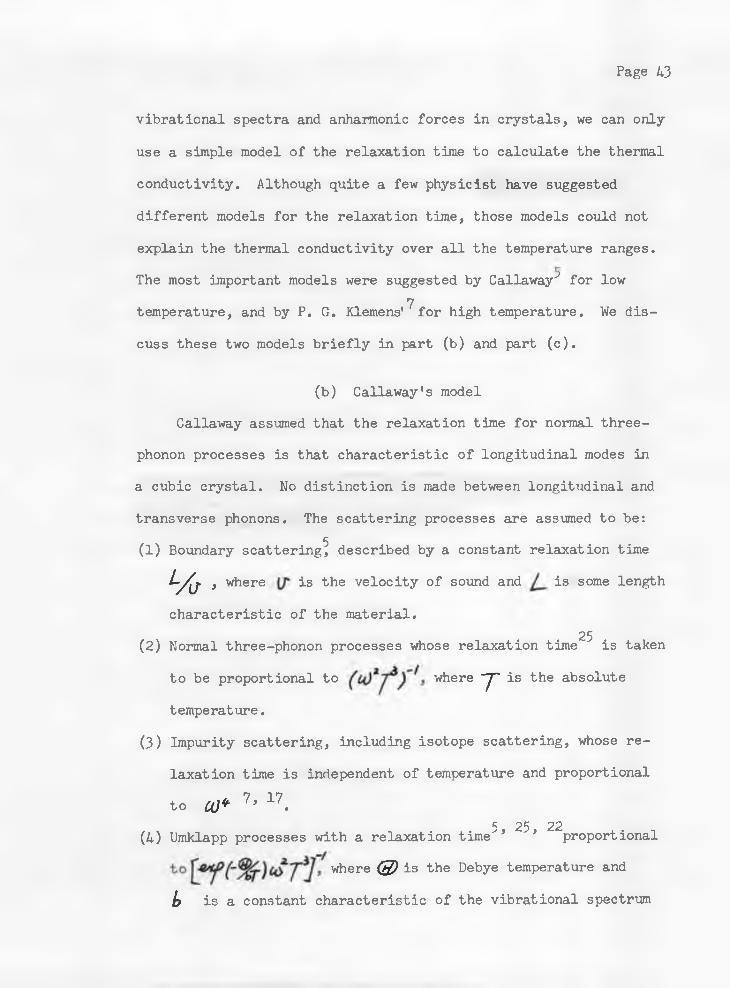
(b) Callaway's model
Callaway assumed that the relaxation time for normal three-
phonon processes is that characteristic of longitudinal modes in
a cubic crystal. No distinction is made between longitudinal and
transverse phonons. The scattering processes are assumed to be:5(1) Boundary scattering, described by a constant relaxation time
LAr , where is the velocity of sound and is some length
characteristic of the material.25(2) Normal three-phonon processes whose relaxation time is taken
to be proportional to where T is the absolute
temperature.
(3) Impurity scattering, including isotope scattering, whose re
laxation time is independent of temperature and proportional
to CO* 7’ 17.5 25 22(4) Umklapp processes with a relaxation time * ’ proportional
where (g? is the Debye temperature and
b is a constant characteristic of the vibrational spectrum

Page 44
of the material. The relaxation time can be written as:
r -' = + (5.13)
(c) Klemens’ model
In I960, Klemens assumed that the relaxation time due to Umklapp7processes is of the form
(5.14)
7 25where If point defects scatter mainly because of their
mass difference, the scattering is described by a relaxation time7
T (5.15)
and
i 7where (X is the atomic volume, (/“ the phonon velocity, and
-e = f c* (/*(5.17)
2 T C - / Y v-t*
and where C*,and^£is the concentration and mass of atoms of type
*£ . Combining the Umklappe-processes and point defect scattering,
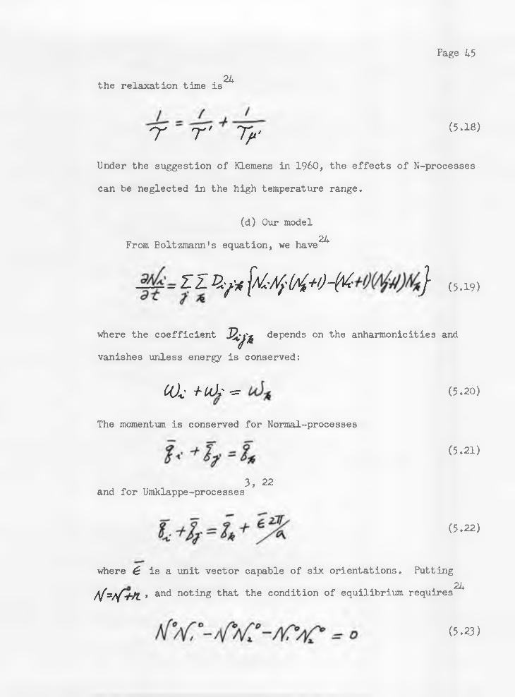
Page 45
the relaxation time is24
r r ' T/s (5.18)
Under the suggestion of Klemens in I960, the effects of N-processes
can be neglected in the high temperature range.
(d) Our model
From Boltzmann's equation, we have24
Z Z Z y * fa-Af- H + O - f a } (5.19)
where the coefficient %/ * depends on the anharmonicities and
vanishes unless energy is conserved:
4 4 + uk ■=The momentum is conserved for Normal-processes
(5 . 20)
(5 .21)
and for Umklappe-processes3, 22
( 5 . 22)
where ^ is a unit vector capable of six orientations. Putting
Af=/{+n , and noting that the condition of equilibrium requires24
(5.23)
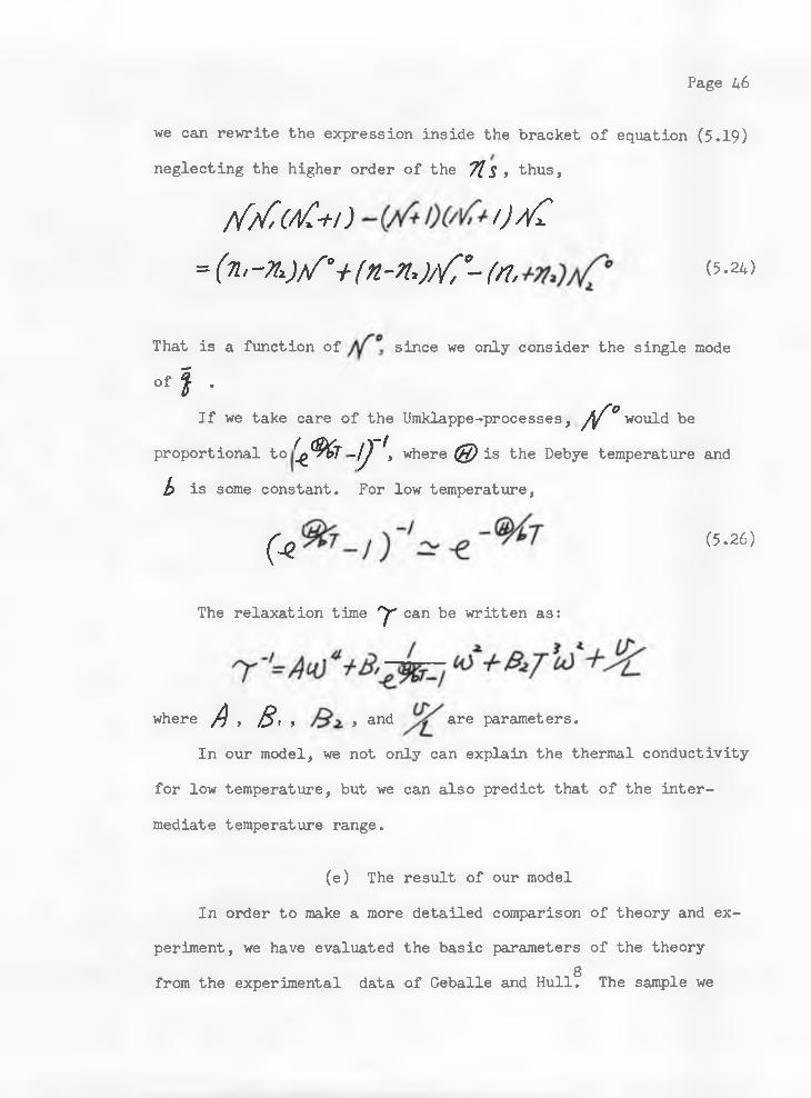
Page 46
we can rewrite the expression inside the bracket of equation (5.19)
neglecting the higher order of the 7ls , thus,/A/Ac/A-h ) -(/ A /)/£= (n, -nx)t/°+ (n-n,)//iB- (n, (5 • 2 4 )
That is a function of since we only consider the single mode
o f f •
If we take care of the Umklappe-processes, y * would be
proportional to ( A r - lJ \ where (£) is the Debye temperature and b is some constant. For low temperature,
C-* (5. 26)
The relaxation time rJ' can be written as:
where A , B ., , and are parameters.In our model, we not only can explain the thermal conductivity
for low temperature, but we can also predict that of the inter
mediate temperature range.
(e) The result of our model
In order to make a more detailed comparison of theory and experiment, we have evaluated the basic parameters of the theory
gfrom the experimental data of Geballe and Hull. The sample we

Page kl
use to calculate the thermal conductivity is normal Ge. Table 5.1
is the comparison of those parameters, /) > 3,» A >tr > and L in the different models of relaxation time for the thermal con
ductivity.
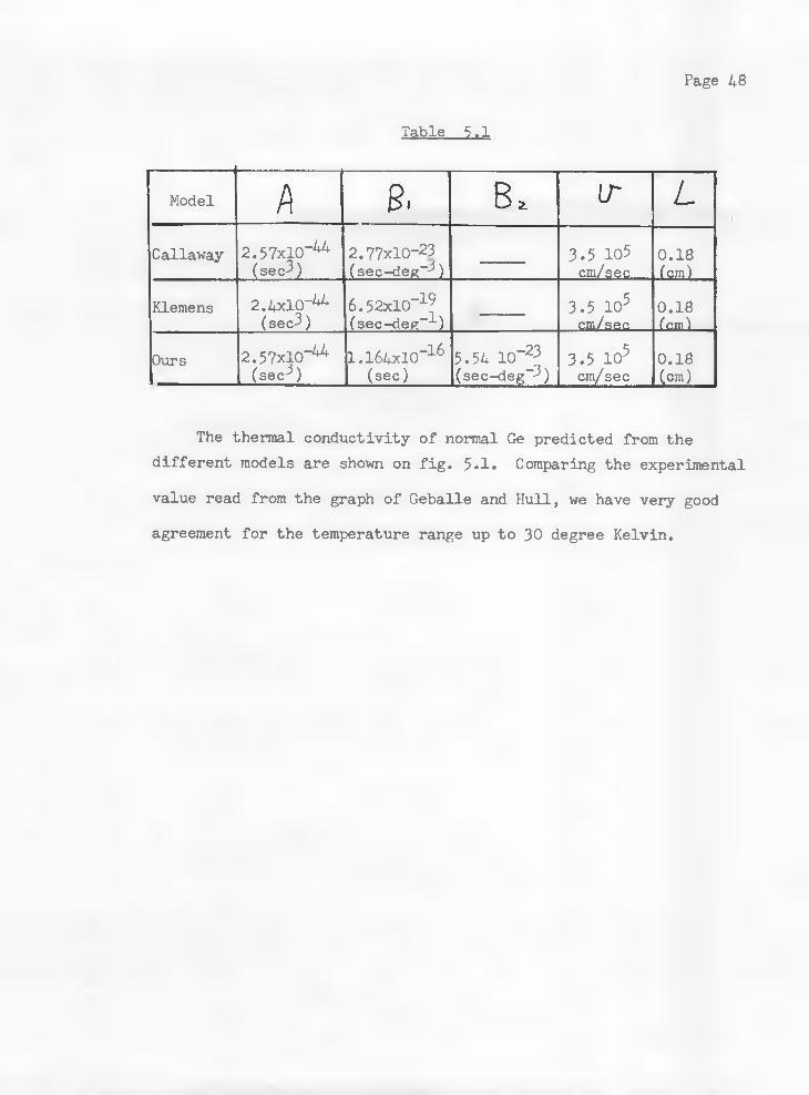
Page 48
Table 5.1
Model f\ g. B, lr L
Callaway 2.57xl0-44(sec3)
2.77x10⁻²³ (sec-deg-- )
3.5 105 cm/sec
0.18(cm)
Klemens 2.4x10"^(sec^)
6.52xlO-19(sec-deg-^)
3.5 105 cm/sec__
0.18(cm)
Ours 2.57xl0-44(sec- )
I.l64xl0-16(sec)
5.54 10~23 (sec-deg-^)
3.5 105 cm/sec
0.18(cm)
The thermal conductivity of normal Ge predicted from the different models are shown on fig. 5.1. Comparing the experimental
value read from the graph of Geballe and Hull, we have very good
agreement for the temperature range up to 30 degree Kelvin.

in w
atts
cm
degr
ees
2 5 10 20 50 Temperature in Degrees Kelvin
Figure 5.1
Thermal Conductivity of Ge
— o— o— : experimental points read from
the graph of Geballe and Hull
— * ' * : predicted from Callaway's model
■— * — x : predicted from our model

SECTION VI
Thermopower
The most sensitive electrical transport property of a metal
is its thermopower which we have briefly discussed in section III.
Several physicists have suggested models to figure out the relaxa-9
tion time and the Fermi surface, then used equation (3.18) to cal
culate the thermopower. Using the power series expansion on the
distribution function, , of electrons in the solid, we present
a new way to figure out the thermopower. For the first order, we
have the same result as equation (3.18).. Furthermore, we can derive
the second order which is important when we have strong fields
across the solid.
Suppose we have a temperature difference, ST- and an electric field, , across the solid. The distribution function, , can
be written as:
[T+S-f, i+ n ) = + ! } ' » • »
where ~J~ is the temperature, £ is energy a n d ^
(6 . 2)
= -e-E ■IT-;;'?'The distribution function, Tit * can be expanded as:
Page 51
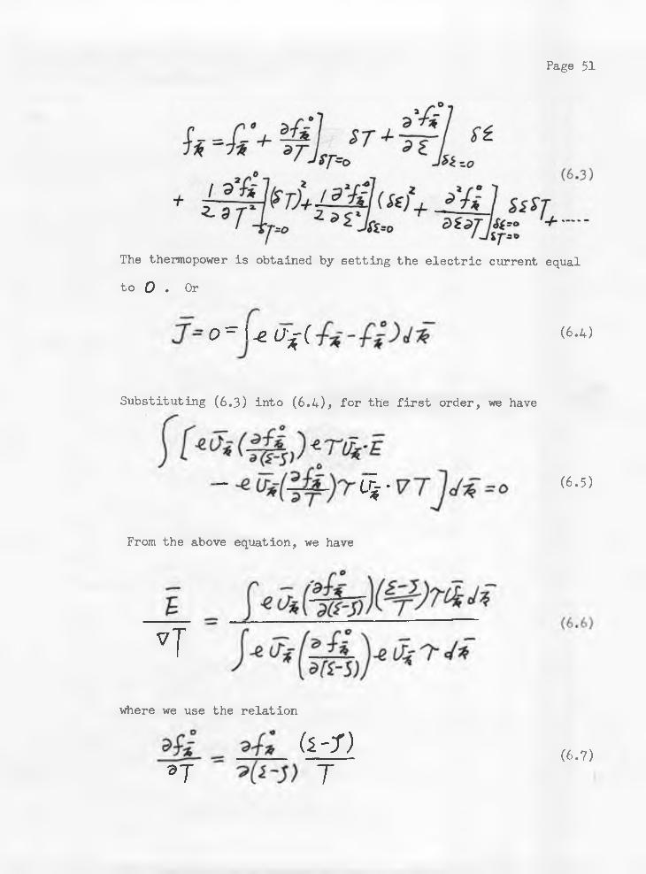
The thermopower is obtained by setting the electric current equal to O . Or
1 = o = Le U f( (6'4)
Substituting (6.3) into (6.4), for the first order, we have
- cj* V T 1 j(6-5)
From the above equation, we have
VJwhere we use the relation
(^11®T ^-5 )T(6.7)

Page 52
Equation (6.6) can be written as:
whereV1 *
(6.8)
(6.9)
To figure out the thermal power, we should calculate the set of
coefficients
of the general theorem as follows:
. These coefficients can be evaluated by means3, 17
where fW is any function of energy, is energy and ^ is the
chemical potential. From the definition of & , we have^’ ^
w / - (6.11)itis the area of the Fermi surface.In the case of , we have
17to consider
/(**)* (U - sM s* ) (6 .12)
which vanishes a t a n d which leaves only'17
Page 53
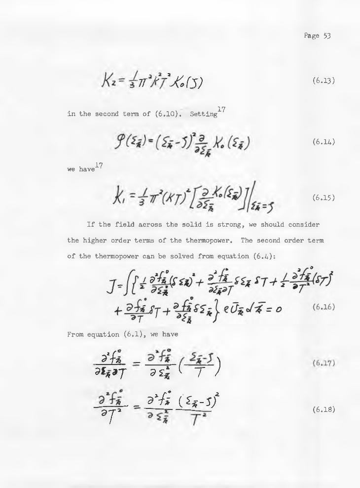
k z = W j< y ‘M f j ) (6-i3>
1 7in the second term of (6.10). Setting
we have"^
If the field across the solid is strong, we should consider
the higher order terms of the thermopower. The second order term
of the thermopower can be solved from equation (6.4):
From equation (6.1), we have
a'-fa _ )9***7 3 si *■ T /
t li_ v '-fi (' U - s ft
(6 .1 4 )
(6 .1 5 )
(6.18)
Page 54
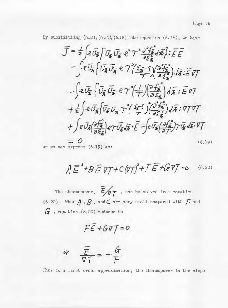
By substituting (6.2),(6J.7), (6J.8) into equation (6.16), we have
if'm « r ( S ^ f J ^ y f:tlTr
-eUi
j
-j^* fW ^ e * t
^ rY ^ M rr) !*■ ;
= oor we can express (6 .1 9 ) as:
(6.19)
j\E*+$E VJ-hCfarf+F ( 6 . 20)
The thermopower, J~ > can s°ive<3 from equation(6.20). When , and C are very small compared with "p- andQf , equation (6.20) reduces to
FE +GrVj = o
or _E_ _ _ J l7T /-
Thus to a first order approximation, the thermopower is the slope

Page 55
of the straight line when we plot jjC versus n - if /) , ,and Q are not small compared to Jl and equation (6.20) is the
set of points on a conic section.
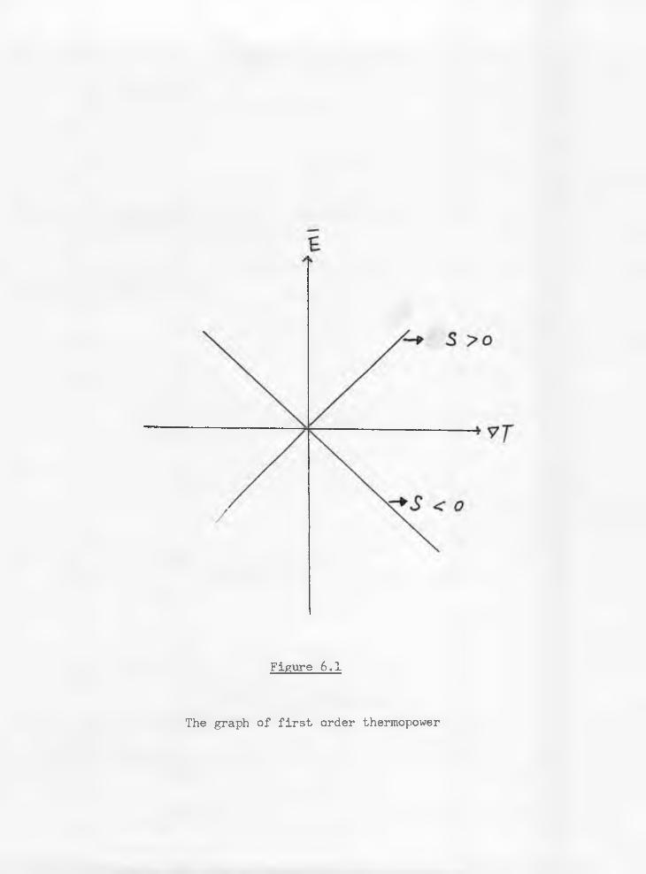
Figure 6.1
The graph of first order thermopower
Page 57
If we consider the case of cubic symmetry, the coefficients,
, and C of equation (6.20)are equal to 0, and the second order of the thermopower is the same as the first order. The ex
pression of electric conductivity, , from equation (3.18), is
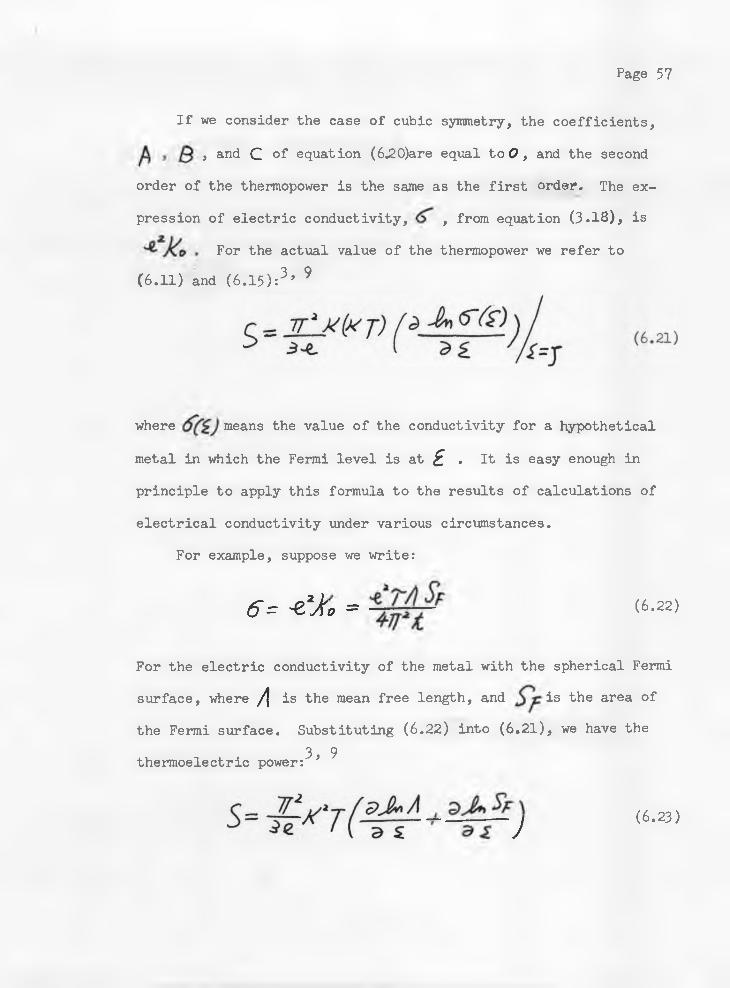
For the actual value of the thermopower we refer to
(6.11) and (6.15):3, 9
where means the value of the conductivity for a hypothetical
metal in which the Fermi level is at £ . It is easy enough in
principle to apply this formula to the results of calculations of
electrical conductivity under various circumstances.
For example, suppose we write:
6 - -etfo = (6 .2 2 )o -
For the electric conductivity of the metal with the spherical Fermi
surface, where /| is the mean free length, and is the area of
the Fermi surface. Substituting (6.22) into (6.21), we have the
thermoelectric power:3, 9
J (6.23)
Page 58
We should expect the first tern in the parenthesis to be positive,
since the more energetic electrons would be less easily scattered
than the slow ones, and thus have longer paths. But the second
term would depend on the detailed geometry of zone. Consider a
Fermi surface expanding into a zone, as in fig. 6.2. Until it
reaches the zone boundary its area increases as £. increases.
Thereafter it will decrease. This term can thus be either positive
or negative, and, in the latter case, may even outweigh the first
term in (6 .2 3 ).
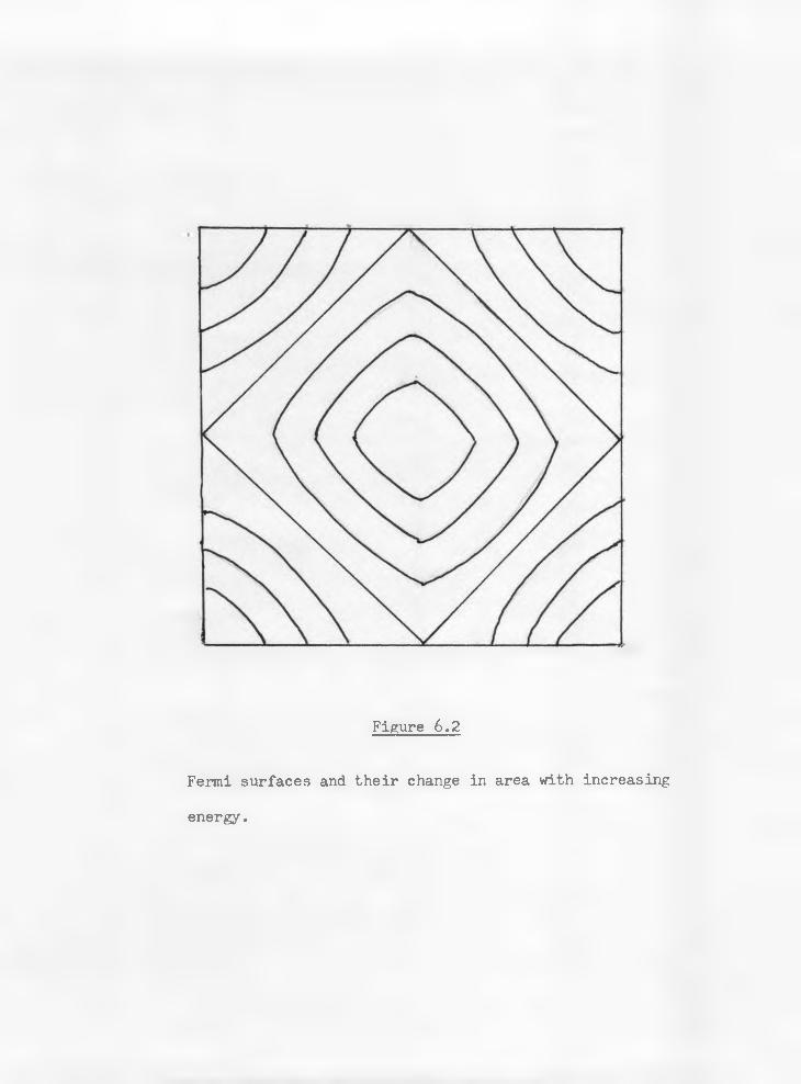
Figure 6.2
Fermi surfaces and their change in area with increasing
energy.

SECTION VII
Conclusion
Onsager's equations are the phenomenological equations which
describe the steady-state case of nonequilibrium thermodynamics,
and are not intended for the non-steady state case. Onsager's
equations have been derived using Hamilton's principle for the
steady-state case in section II, by identifying the proper
Lagrangian function. We pointed out that the variational principle
is a unifying principle for understanding the physical world, al
though we only derived the equations for the steady-state case.
If a system is subject to two thermodynamic forces, such as
the electric potential gradient W and a temperature gradient
can be reduced to three by using Onsager's reciprocal relationship,
have been related to the therital conductivity, electrical conductiv-A
ity, and thermopower. One set of coefficients can be derived from
the other through equations (3.17) and (3.18) . Although, in
principle we can measure Onsager's coefficients, the easier way to
calculate Onsager's coefficients is in terms of the directly meas
, the electric current J and the heat current V can
be obtained from Onsager's equations, as seen in equation (1.1)
The four coefficients, , U , Z v and Z ,
In section III, these three independent coefficients
urable thermal coefficients.
Page 61
The electrons moving in the solid will be influenced by the
lattice structure, causing electrical resistivity. In quantum
mechanical language, this is the interaction between an electron
in a particular state described by a particular wave function, and
a lattice vibration, described by a phonon eigenstate. The phonon
disturbs the lattice, moving some of the atoms away from the posi
tions they should have according to the "official" structure of
the crystal. An electron is affected by the change of the posi
tion, and is thus liable to be deflected, or scattered, out of its
accustomed course. The process is much like that by which phonons
interact. A longitudinal vibration, for example, compresses or
expands the lattice at various points. At these points the effec
tive electrostatic potential acting on this electron is changed,
and there is the possibility of scattering. The scattering is
characterized by a relaxation time, which describes the average
time between two successive collisions. This relaxation time is
needed to solve the Boltzmann equation, which describes this scatt
ering.
The relaxation time has been related to the transition rate
through equation (4.1) . Although Fermi's-Golden rule 2 has been
used successfully to derive the transition rate, we present another
convenient way to derive the transition rate, by using the equation
of motion as mentioned in section IV. The first order approximation
is in agreement with Fermi's-Golden rule 2. When the transition
rate between the second and third energy bands is large, the second
Page 62
order term, L v , * r j , should be considered. Although we only-
considered a pure metal, other materials can be tested by this
method.
We have seen that the thermal energy of the crystal consists
of waves which travel near the velocity of sound, and which are
capable of transporting energy. In the harmonic approximation the
waves travel freely without attenuation, and therefore have an un
limited free path. In reality their free path is limited by:
(a) the anharmonic terms,
(b) impurities and imperfections in the crystal, and
(c) the finite dimensions of the crystal.
The anharmonic approximation can be interpreted as the three-phonon
scattering processes, Normal-processes and Umklappe-processes,
which have been discussed in section V.
To calculate the thermal conductivity, we need to assume a
relaxation time rrfV . The relaxation time we have assumed in
section V provides very good agreement with experimental results for
the temperature range up to 30° K. The Normal-process seems to be
very important for the temperature around 20° K for Ge. If we omit
the Normal-processes for the temperature range above the Debye
temperature, the model for the relaxation time used in section V
also gives the same result as that of the Klemens' model. If we
can determine the parameter, B, , of the Normal-processes such
that it is approximately equal to 0 for the high temperature range,
and equal to the value we have for the low temperature in section V,
Page 63
then we can explain the thermal conductivity over all temperature5ranges.
Thermopower concerns the direct generation of an e.m.f. by
thermal means. This involves subjecting a conductor to a tempera
ture gradient. Physically, the phenomenon arises because electrons
at the hot end of such a conductor can find states of lower energy
at the cold end, to which they diffuse, setting up an electric
potential difference between the two ends. Looked at another way,
an electron can be considered to have energy £ which, because of
the temperature gradient, is dependent on its position Y in the
metal. Thus, a force acts on the electron, given by 7 ^ - e v V -
Being capable of movement through the metal, electrons accumulate
at the cold end of the conductor, as before. Furthermore, the mean
conduction electron energy of one material will almost certainly
differ from that in another, and this produces another thermoelec
tric effect. When an electric current is passed through a junction
of two dissimilar materials, heat will either be produced or be
absorbed at the junction. This is known as the Peltier effect.
The first order expression for the thermopower has been known
and used for a long time. Using a power series expansion for the
distribution function of electrons, , we obtain the same re
sult as the traditional approach in first order approximation.
We also obtain an expression for the thermppower for the second
order approximation. The second order of the thermopower depends
on the coefficients, A, B, and C, in equation (6.20) . It is not
Page 64
difficult to obtain A, B, and C in principle. But the Fermi sur
face is too complicated to get A, B, and C exactly, so an approxi
mation for the Fermi surface is assumed in order to calculate those
coefficients.

Page 65
BIBLIOGRAPHY
1. De C-root, S. R. and Mazur, P., Nonequilibrium Thermodynamics,North-Holland, Amsterdam, 1 9 6 3 .
2. Morse, Philip M. and Feshbach, Herman, Method of TheoeticalPhysics, McGraw-Hill, New York, 1953.
3. Ziman, J.M., Electrons and Phonons, The Clarezdon Press,Oxford, I960.
4. Bardeen, J., Phys. Rev. 52, 688, 1973.
5. Callaway, Joseph, Phys. Rev. 113, 1046, 1959.
6. Carruthers, Peter, Rev. of Modern Phys. 33, 92, 1961.
7. Klemens, P. G., Phys. Rev. 119, 507, I960.
8. Gevalle, T. H. and Hull, G. W., Phys. Rev. 110, 773, 1958.
9. Barnard, R. D., Thermoelectricity in Metals and Alloys, HalstedPress, London, 1972.
10. Goldstein, H., Classical Mechanics, Addison-Wesley, Massachusetts, 1967.
11. Marion, J. M., Classical Electromatnetic Radiation, AcademicPress, New York, 1965.
12. Notes of Classical Mechanics at Creighton University.
13. Ziman, J. M., Canadian J. of Phys. 34, 1264, 1965.
14. Ter Haar, D., Elements of Statistical Mechanics, Rinehart,New York, 1954.
15. Onsager, L., Phys. Rev. 37, 405; 38, 2265, 1931.
16. Jeans, J. H., Electricity and Magnetism, 4th ed. CambridgeUniversity Press, 1920.
17. Ziman, Principle of Solid State Physics, Cambridge University Press, 1972
Harrison, W. A., Solid State Theory, McGraw-Hill, New York, 1970.
18.
Page 66
19. Nordheim, L. W., Ann. d. Physik 9, 607, 1931.
20. Sommerfeld, A. and Bethe, H. A., Handbuch der Physik. Vol.24, II, Berlin, 1933.
21. Schiff, L. I., Quantum Mechanics. McGraw-Hill, New York, 1968.
22. Peierls, R. E., Quantum Theory of Solid, Oxford UniversityPress, Oxford, 1955.
23. Mott, N. F, and Jones, H., Theory of the Properties of Metalsand Alloys, Clarendon Press, Oxford, 1936.
24. Klemens, P. G., Proc. Roy. Soc. A208, 108, 1951.
25. Conyers Herring, Phys. Rev. 95, 954, 1954.
26. De Groot, Y. R., Thermodynamics of Irreversible ProcessesNorth-Holland, 1951-