thesis miguel Ángel lago
TRANSCRIPT


A new approach for the in-vivocharacterization of the
biomechanical behavior of thebreast and the cornea
Author: MIGUEL ÁNGEL LAGO ÁNGEL
Supervisor: Dr. Carlos Monserrat ArandaSupervisor: Dr. María José Rupérez Moreno
DEPARTAMENTO DE SISTEMAS INFORMÁTICOS Y COMPUTACIÓN
October, 2014


The research derived from this doctoral thesis has been par-tially funded by MINECO (INNPACTO, IPT-2012-0495-300000)through the research project ECTASIA.
The work of Miguel Ángel Lago Ángel to carry out this re-search and to elaborate this dissertation has been supported bythe Spanish Government under the FPU Grant AP2009-2414.


AgradecimientosLlegando al final del camino, uno se pregunta si ha valido la
pena el tiempo y esfuerzo invertido y la respuesta es sí. Desdeaquel primer día que empecé esta aventura, hasta el último deellos, ésta ha sido, sin duda, la experiencia más enriquecedora demi vida. Todo lo aprendido y todo vivido, son cosas que formaránparte de mí y que siempre recordaré con especial alegría.
El trabajo que hay en estas páginas no es algo individual, puesdebo dar las gracias a todas las personas que han influido en él enmayor o menor medida. Ha sido mucha la gente que he tenidoel placer de conocer durante estos años y que no han dejado desorprenderme día a día, empezando por mis dos directores detesis, Carlos y María José, que han sido mis maestros durante estosaños y con los que siempre estaré en deuda por todos los consejosy ayuda que me han aportado, no sólo en el ámbito académico.Pero, sobre todo, por la paciencia que han demostrado en muchasde las discusiones que hemos tenido.
Muchísimas gracias a mis compañeros de trabajo con los quehe compartido tantos momentos y anécdotas: Rober, Fer, Sandra,Eliseo, Juanjo, Pablo, Álex y, especialmente, a mi segundo de abordo y amigo Fran, por la ayuda y consejos que han sido crucialespara que esta tesis saliera adelante.
I would also like to thank Andrew Maidment and, specially,Predrag Bakic for his enthusiastic support this last year and duringmy stay at the University of Pennsylvania. I could have neverthought in a better place to stay.
Finalmente, gracias a mis padres Marina y Jesús y a mi her-mano Óscar, además de todos los amigos, viejos y nuevos, quehan visto como aquella decisión que hizo que me dedicara a la in-vestigación ha dado por fin sus frutos. Una carrera investigadoraque no sé a dónde me llevará a partir de ahora. Es un emocionantemisterio, el no saber qué me deparará el futuro, que me intriga yestoy deseando descubrir.


That quite definitely is the answer. I think the problem, to be quite honestwith you, is that you’ve never actually known what the question is.
Deep Thought, The Hitchhiker’s Guide to the GalaxyDouglas Adams


AbstractThe characterization of the mechanical behavior of soft living tis-sues is a big challenge in Biomechanics. The difficulty arises fromboth the access to the tissues and the needed manipulation in orderto know their physical properties. Currently, the biomechanicalcharacterization of organs is mainly performed by testing ex-vivotissue samples or by means of indentation tests. In the first case,the obtained behavior does not represent the real response of theorgan. In the second case, it is only a representation of the mechan-ical response of the indented areas. The purpose of the researchreported in this thesis is the development of a methodology forthe in-vivo characterization of the biomechanical behavior of twodifferent organs: the breast and the cornea. The proposed method-ology allows the in-vivo characterization of their biomechanicalbehavior using medical images.
The research reported in this thesis describes a new approachfor the in-vivo characterization of the biomechanical behavior ofthe breast and the cornea based on the estimation of the elastic con-stants of their constitutive models. This estimation is performedusing an iterative search algorithm which optimizes these param-eters. The search is based on the iterative variation of the elasticconstants of the model in order to increase the similarity betweena simulated deformation of the organ and the real one. The sim-ilarity is measured by means of a volumetric similarity functionwhich combines overlap-based coefficients and distance-basedcoefficients.
In the case of the breast, the methodology is based on the sim-ulation of the compression of the breast during an MRI-guidedbiopsy. The validation was performed using breast software phan-toms. Nevertheless, this methodology can be easily transferredinto its use with real breasts. In the case of the cornea, the method-ology is based on the simulation of the deformation of the humancorneas due to non-contact tonometry.


ResumenLa caracterización del comportamiento biomecánico del tejidovivo representa un gran reto en biomecánica. La dificultad radicatanto en el complicado acceso a los tejidos como en su manipu-lación a la hora de conocer sus propiedades físicas. Actualmente,la caracterización biomecánica de los órganos se realiza utilizandomuestras de tejido ex-vivo que son sometidas a experimentos detracción y compresión o mediante tests de indentación. En elprimer caso, la respuesta obtenida no representa necesariamenteel comportamiento real del órgano. En el segundo caso, sólo esuna representación de la respuesta mecánica de la zona estudiada.La investigación presentada en esta tesis tiene como propósito eldesarrollo de una metodología para la caracterización in-vivo delcomportamiento biomecánico de dos órganos diferentes: la mamay la córnea. La metodología propuesta permite la caracterizaciónin-vivo de su comportamiento biomecánico específico del pacienteutilizando imágenes médicas.
La investigación presentada en esta tesis describe una nuevaaproximación para la caracterización in-vivo del comportamientobiomecánico de la mama y de la córnea basada en la estimaciónde las constantes elásticas de sus modelos constitutivos. La es-timación se realiza mediante un algoritmo que optimiza estosparámetros. La búsqueda está basada en la variación iterativa delas constantes elásticas del modelo con el fin de incrementar lasimilitud entre la deformación del órgano simulada y su deforma-ción real. La semejanza se mide mediante una función de similitudvolumétrica la cual combina medidas de solape y distancia.
En el caso de la mama, la metodología está basada en la simu-lación de la compresión de la mama durante una biopsia guiadapor resonancia magnética. La validación se realizó utilizandophantoms software de mama. Esta metodología se puede trasladarfácilmente a mamas reales. En el caso de la córnea, la metodologíase basa en la simulación de la deformación de la córnea humanadurante el proceso de tonometría sin contacto.


ResumLa caracterització del comportament biomecànic del teixit viu rep-resenta un gran repte en biomecànica. La dificultat ve tant delcomplicat accés als teixits com de la necessitat de manipulació pertal de conèixer les seues propietats físiques. Actualment, la carac-terització biomecànica dels òrgans és realitzada utilitzant mostresde teixit ex-vivo o mitjançant proves de tracció i compressió. En elprimer cas, la resposta obtinguda no representa necessàriamentel comportament real de l’òrgan. En el segon cas, només és unarepresentació de la resposta mecànica de la zona estudiada. Lainvestigació presentada en aquesta tesi té com a propòsit el desen-volupament d’una metodologia per a la caracterització in-vivo delcomportament biomecànic de dos òrgans diferents: la mama i lacòrnia. La metodologia proposta permet la caracterització in-vivodel seu comportament biomecànic específic per a cada pacientutilitzant imatges mèdiques.
La investigació presentada en aquesta tesi descriu una novaaproximació per a la caracterització in-vivo del comportamentbiomecànic de la mama i de la còrnia basada en l’estimació de lesconstants elàstiques dels seus models constitutius. L’estimació esrealitza mitjançant un algorisme de cerca iterativa que optimitzaaquests paràmetres. Hi està basada en la variació iterativa de lesconstants elàstiques del model per tal d’incrementar la semblançaentre una deformació simulada de l’òrgan i el seu comportamentreal. La semblança és mesura mitjançant una funció de simili-tud volumètrica la qual combina coeficients de solapament i dedistància.
En el cas de la mama, la metodologia està basada en la simu-lació de la compressió de la mama durant una biòpsia guiada perressonància magnètica. La validació es va realitzar utilitzant phan-toms virtuals de mama. Aquesta metodologia es pot traslladarfàcilment per usar-se amb mames reals. En el cas de la còrnia, lametodologia es basa en la simulació de la deformació de la còrniahumana durant el procés de tonometria sense contacte.


Contents
1 Introduction 1
1.1 Objectives . . . . . . . . . . . . . . . . . . . . . . . . 3
1.2 Main contributions . . . . . . . . . . . . . . . . . . . 5
1.3 Outline . . . . . . . . . . . . . . . . . . . . . . . . . . 7
2 Context and background 9
2.1 Introduction to tissue characterization . . . . . . . . 9
2.2 Characterization of the breast tissues . . . . . . . . . 12
2.3 Characterization of the corneal tissue . . . . . . . . . 15
2.4 Conclusions . . . . . . . . . . . . . . . . . . . . . . . 18
3 Materials and methods 19
3.1 Biomechanical modeling of soft tissue . . . . . . . . 20
3.1.1 Finite Element Method . . . . . . . . . . . . . 21
3.1.2 Hyperelasticity . . . . . . . . . . . . . . . . . 23
i

3.2 Optimization by genetic heuristics . . . . . . . . . . 26
3.2.1 Genetic operators . . . . . . . . . . . . . . . . 27
3.2.2 GA outline . . . . . . . . . . . . . . . . . . . . 28
3.3 Similarity coefficients . . . . . . . . . . . . . . . . . . 30
3.3.1 Overlap and distance coefficients . . . . . . . 31
3.3.2 Analyzing the performance of the coefficients 34
3.3.3 Geometric Similarity Function . . . . . . . . 41
3.4 Conclusions . . . . . . . . . . . . . . . . . . . . . . . 44
4 Characterization of the biomechanical behavior of the
breast 45
4.1 Breast anatomy . . . . . . . . . . . . . . . . . . . . . 46
4.2 Breast imaging systems . . . . . . . . . . . . . . . . . 47
4.2.1 X-ray Mammography . . . . . . . . . . . . . 49
4.2.2 Magnetic Resonance . . . . . . . . . . . . . . 50
4.3 Software breast phantoms . . . . . . . . . . . . . . . 53
4.4 Study of the mesh quality . . . . . . . . . . . . . . . 58
4.4.1 Materials and Methods . . . . . . . . . . . . 60
4.4.2 Simulation of the mammographic compres-
sion . . . . . . . . . . . . . . . . . . . . . . . . 64
4.4.3 Results of the mesh quality analysis . . . . . 66
4.4.4 Discussion . . . . . . . . . . . . . . . . . . . . 72
4.5 Biomechanical modeling of the breast tissues . . . . 76
4.5.1 Hyperelastic anisotropic model of the breast 77
4.5.2 Estimation of the biomechanical properties . 79

4.5.3 Software phantom generation . . . . . . . . . 80
4.5.4 Boundary conditions and contact . . . . . . . 80
4.5.5 Search algorithm . . . . . . . . . . . . . . . . 81
4.5.6 Results . . . . . . . . . . . . . . . . . . . . . . 82
4.5.7 Discussion . . . . . . . . . . . . . . . . . . . . 86
4.6 Conclusions . . . . . . . . . . . . . . . . . . . . . . . 92
5 Characterization of the biomechanical behavior of the
cornea 95
5.1 Cornea anatomy . . . . . . . . . . . . . . . . . . . . . 96
5.2 Biomechanical model of the cornea . . . . . . . . . . 97
5.3 Estimation of the biomechanical properties . . . . . 99
5.4 Search algorithm . . . . . . . . . . . . . . . . . . . . 102
5.5 Results . . . . . . . . . . . . . . . . . . . . . . . . . . 104
5.6 Discussion . . . . . . . . . . . . . . . . . . . . . . . . 107
5.7 Conclusions . . . . . . . . . . . . . . . . . . . . . . . 110
6 Conclusions 113
6.1 Summary of contributions . . . . . . . . . . . . . . . 114
6.2 Future work . . . . . . . . . . . . . . . . . . . . . . . 115
6.3 Final considerations . . . . . . . . . . . . . . . . . . . 116
Bibliography 119


Chapter 1
Introduction
The medical industry is moving towards the simulation of the realbehavior of human organs. Being able to simulate the mechanicalresponse of the human organs can be useful to determine theirreactions in a future intervention. Surgical simulation systemsprovide surgeons with virtual environments that serve as a guideduring an intervention, simulating critical what-ifs scenarios. Theycan also be used to train the skills of the novice surgeons. The bigchallenge of these systems is to guarantee a simulation as similaras possible to the real behavior of the organ.
Patient-specific biomechanical models are the current tendencyin surgical simulation. Being able to provide the surgeon with anaccurate and specifically designed model of the organ to be treatedcan be very helpful for many medical applications such as surgicalplanning, surgical guidance, image registration, and diagnosis.However, constructing patient-specific models of organs is not
1

2 CHAPTER 1. INTRODUCTION
an easy task. The internal and external organs of the body aresubjected to many loads that affect their mechanical behavior.Therefore, in order to understand the response of tissue to a giveninteraction, it is necessary to determine its mechanical properties.
Living organs have the ability to undergo large deformationsand, even so, recover the original configuration after a certainperiod of time. This behavior can be characterized as a biomechan-ical problem. The European Society of Biomechanics defines theBiomechanic Science as “the study of forces acting on and generatedwithin a body and of the effects of these forces on the tissues, fluidsor materials used for diagnosis, treatment or research purposes”. Theinherent heterogeneous composition of the organs, as well as thecomplexity of their internal structures, confer this type of tissuesa high malleability. This makes the modelization of its behaviorin a virtual environment very hard. Besides, the high variabilityamong individuals and the difficulty of measuring the mechanicalresponse represents the main challenge.
A trustful biomechanical constitutive model of an organ needsto mimic not only its size and shape but also its mechanical be-havior, tissue distribution and interactions with the neighboringtissues. Ideally, all this data must be inferred without any inter-vention, from medical images like Computerized Tomography(CT) or 3D Magnetic Resonance Images (MRI), thus increasing thedifficulty of achieving a realistic physical model for the organs ofeach patient. Previous works have characterized the mechanicalbehavior of organs by means of ex-vivo experiments. However,these results are not realistic enough since the samples becomestiffer due to the fluid loss when they are extracted. There are

1.1. OBJECTIVES 3
also studies that measured the mechanical response of the organsin-vivo, with the disadvantage of characterizing it only in somespecific points besides needing invasive interventions. Therefore,there is a real need of developing new methodologies that allowthe in-vivo characterization of the whole organ behavior whichmake use of medical images, thus avoiding invasive interventionssuch as open surgery.
This thesis presents a new approach for the in-vivo characteri-zation of the biomechanical behavior of two different organs: thebreast and the cornea. In particular, a methodology based on theestimation of the elastic constants of the constitutive biomechani-cal models is proposed for each organ. This estimation is carriedout as a parameter optimization problem in which the input pa-rameters are iterated over the given fit function to be minimized.The considered function measures the volumetric similarity, in-cluding the internal tissue distribution of all the tissues, betweena deformation of the organ simulated by a biomechanical model,and the real response of the organ. Genetic heuristics were appliedin order to guide the search algorithm since this type of heuristicsare suitable to optimize complex functions that may present manylocal minima.
1.1 Objectives
The main objective of the work presented in this thesis wasto develop a methodology for the in-vivo characterization of thebiomechanical behavior of the breast and the cornea. Specifically,the methodology was aimed to estimate in-vivo the patient-specific

4 CHAPTER 1. INTRODUCTION
elastic constants of the proposed constitutive models for theseorgans.
Additionally, from this main objective, several secondary ob-jectives arose.
First of all, in order to quantify the error committed by a biome-chanical model in the simulation of the biomechanical behaviorof a whole organ, several coefficients for medical image analy-sis were analyzed. This study involved both overlap-based anddistance-based coefficients. The aim was to select the set of coeffi-cients which best quantified this error in order to be used as a fitfunction in the parameter estimation.
The methodology had to be able to estimate the patient-specificelastic constants of the biomechanical models of the breast and thecornea. To carry out this estimation, an iterative algorithm thatsearches for the minimum of the proposed fit function by changingthe input parameters is needed. This parameter optimization mustavoid being trapped in local minima or discontinuities. Therefore,a genetic heuristic approach was selected in order to drive theiterative search algorithm and to find the optimum parameters.
The estimation of the elastic constants of the constitutive biome-chanical models chosen for the breast and the cornea was carriedout by an iterative search algorithm. The automatic nature of thisalgorithm requires a realistic simulation as well as the guarantee ofthe convergence of the finite element method used to simulate thedeformations that the organs undergo. Therefore, a study of theimpact of the mesh quality in these simulations was performed.

1.2. MAIN CONTRIBUTIONS 5
Due to the high complexity of its internal tissue distribution, thestudy was carried out for the case of the breast
In order to characterize in-vivo the biomechanical behavior ofthe breast tissues, an experiment involving a controlled deforma-tion of the breast had to be chosen. This was the mammographiccompression that the breast undergoes during an MRI-guidedbiopsy. The mammographic compression was modeled as a con-tact problem. The breast tissues were segmented, meshed andplaced between two rigid plates on which a controlled force wasapplied to compress the finite element mesh. The simulated defor-mation of the breast was then compared to the real one in order toestimate the elastic constants of the selected model.
In the case of the cornea, another experiment that provided acontrolled deformation of the cornea had to be simulated. Theimages taken from a camera during the non-contact tonometryperformed by the Corvis® ST device were used as the target defor-mation. A comparison of the real and simulated deformation wasperformed in order to estimate in-vivo the elastic constants of theproposed model. Analogously to the breast case, a finite elementmesh was constructed and the air jet from the tonometer wasapplied as a pressure on the cornea surface to get the simulateddeformation that was compared to the real one.
1.2 Main contributions
Two coefficients for medical image analysis that measurethe similarity between volumes were selected to comparethe organ simulated deformation to the real one: the Jac-

6 CHAPTER 1. INTRODUCTION
card coefficient, which measures the overlap between twovolumes; and the Modified Hausdorff Distance, which isrelated to the distance between the surfaces of two volumes.These coefficients proved to be suitable to evaluate the errorcommitted by the biomechanical simulation of a physicaldeformation.
The mesh quality study carried out on the breast modelshowed that a mesh created by regular elements provided asgood results as a mesh with elements adapted to the internaltissue distribution of the breast. Moreover, the elements ofthe regular mesh had better quality, easier convergence andfaster solver times.
The biomechanical behavior of the breast was characterizedusing software breast phantoms with an error under 10%.This was performed by the estimation of the elastic constantsof the constitutive equations that govern the behavior of itsthree main tissues. The proposed methodology can be easilyapplied to real cases.
Finally, the methodology was also applied to characterizethe biomechanical behavior of the in-vivo tissue of the cornea.Taking advantage of the tonometry procedure, the patient-specific elastic constants of a hyperelastic second-order Og-den model were estimated for 24 real corneas of 12 patientswith an error under 5%.

1.3. OUTLINE 7
1.3 Outline
This dissertation is organized in 6 chapters, starting with theintroductory Chapter 1, which includes the objectives and maincontributions of this thesis.
In Chapter 2, the background and context where the thesis isframed is detailed, including a literature review on characteriza-tion of the breast, and the corneal tissues.
Chapter 3 establishes the base of the methodology for the in-vivo characterization of the biomechanical behavior of the twoorgans, including the biomechanical modeling, the descriptionof the genetic heuristics, and the presentation of the similaritycoefficients.
Chapter 4 describes the application of the methodology to thebreast tissues and its validation using software phantoms. Inthis chapter, the breast anatomy is detailed along with both theselected constitutive model, and the software phantoms. Thischapter also includes the study of the mesh quality.
In Chapter 5, the application of the methodology to real corneasis described. The cornea anatomy and the biomechanical modelingof the tonometry procedure are detailed, as well as the processdeveloped to estimate the elastic constants of the constitutivemodel that describes the cornea behavior.
Finally, Chapter 6 presents the final conclusions of this disser-tation, the future work, and the resulting publications.

Chapter 2
Context and background
This chapter reviews previous works on the biomechanical char-acterization of soft tissue. Specifically, the literature about thecharacterization of the breast and the cornea is detailed in orderto establish the framework of this thesis.
2.1 Introduction to tissue characterization
In 1972, Fung proposed what is considered the first theorythat describes the phenomenological temporal mechanics of thesoft tissue. This theory, called the quasi-linear viscoelastic theory,separates the mechanical behavior of the tissue in two compo-nents: the nonlinear time-independent hyperelastic componentand the linear time-dependent component. This model reducesthe formulation of the mathematical model easing the simulationon a computer and, specifically, allowing methods like the Finite
9

10 CHAPTER 2. CONTEXT AND BACKGROUND
Element Method (FEM), to simplify its resolution.
First steps in biomechanical characterization of human tissuecan be found in early 70’s. The first experiments performed uniax-ial tensile tests to obtain the mechanical response of soft tissues[Clark, 1973; Ghista and Rao, 1973; Lanir and Fung, 1974]. In atensile test, the sample is gripped by the so-called clamps anda force is applied in order to measure the force feedback causedby the tension. The measured force can be used to infer tissueproperties like elasticity or compressibility. However, uniaxialtensile tests are not accurate enough to completely estimate theanisotropic behavior of the soft tissue [Fung, 1974; Chew et al.,1986; May-Newman and Yin, 1995; Billiar and Sacks, 2000; Zhaoet al., 2011].
Moving on to more complex tissues, those which have ananisotropic behavior need different experiments like biaxial tensiletests. In this type of tests, the sample is subjected to two forces indifferent directions, thus obtaining two reactions that allows thecharacterization of the tissue anisotropy. However, as with uniax-ial tests, the characterization is limited to the considered portionof tissue [Nielsen et al., 2002]. Furthermore, the inhomogeneityof biological tissue causes this type of tests to characterize theaverage behavior of the collected sample, or the region subjectedto the stress.
Nowadays, there is an increasing interest in characterizing thebiomechanical behavior of the living tissues since, due to the wa-ter loss, the ex-vivo samples becomes stiffer and their mechanicalproperties vary significantly. It is also important to highlight the

2.1. INTRODUCTION TO TISSUE CHARACTERIZATION 11
difficulty of extracting samples of some specific tissues from thebody as well as the severe impact that the extraction of the tissuescould have on a patient. Additionally, the variability among sam-ples (for different patients and for the same patient in differenttimes), and the inherent conditions of the measuring techniquesentail the necessity of creating more specific models for each pa-tient [Gee et al., 2010; Miller and Lu, 2013]. In this direction, workslike [Carter et al., 2001; Samur et al., 2005; Nava et al., 2008] per-formed in-vivo indentation tests on animal organs thus measuringtheir specific mechanical properties.
In an indentation test, a force is applied on a small region ofthe tissue and the material properties are determined by mea-suring the force feedback [Gow and Vaishnav, 1975; Hori andMockros, 1976; Zheng and Mak, 1996; Han et al., 2003; Samaniand Plewes, 2004]. As well as with tensile tests, the viscoelasticity,time-dependent response of the tissue, can be determined by thesetests [Humphrey et al., 1991; Samani and Plewes, 2004; O’Haganand Samani, 2009; Martínez-Martínez et al., 2013a]. The anisotropyof the tissue can also be obtained by means of using an asymmetricindentation device [Jeffrey, 2004] as well as the characterization offiber-reinforced materials [Cox et al., 2008]. However, the problemwith all these tests is that they only characterize the biomechani-cal properties of the small area where the device is applied, withthe result of being only valid for that region and not necessarilyrepresenting the behavior of the whole organ.

12 CHAPTER 2. CONTEXT AND BACKGROUND
2.2 Characterization of the breast tissues
The simulation of the mechanical behavior of the breast isbecoming a very relevant field in the last years owing to its mainrole in an important number of biomedical applications related tosurgical simulations [Tanner et al., 2006a; del Palomar et al., 2008;Hsu et al., 2011; Solves Llorens et al., 2012], surgical guidance[Carter et al., 2008; Han et al., 2011] or cancer diagnosis [Ruiteret al., 2006; Pathmanathan et al., 2008; Rajagopal et al., 2010]. Theseapplications involve large deformations of the internal tissues ofthe breast such as mammographic compression or gravity loadingdeformation, which are usually modeled using the Finite ElementMethod (FEM).
One of the main challenges when modeling the biomechani-cal behavior of organs like the breast is to create patient-specificmodels that improve the realism and accuracy in a reasonablecomputational time. However, the estimation of the biomechan-ical properties of the living tissues is not straightforward. Themeasurement of these properties is usually a complex task sincethe behavior of the tissues is highly variable among individuals.In the case of the breast, there are mainly four tissues whose be-havior must be modeled, namely: skin, fat, glandular tissue andthe Cooper’s ligaments. Each of them has its own biomechanicalproperties that must be estimated for each patient in order to buildan accurate model of the whole breast. In the case of the Cooper’sligaments, since they are not visible in any image scanner modal-ity, its influence on the breast is usually considered implicitly inthe fat tissue.
2.2. CHARACTERIZATION OF THE BREAST TISSUES 13
The behavior of the breast tissue has already been measuredwith ex-vivo experiments by indentation or aspiration tests [Gefenand Dilmoney, 2007; O’Hagan and Samani, 2009]. Unfortunately,the behavior of the samples outside the body is more rigid andit does not correspond to the mechanical properties of the livingorgan.
Elastography is a common method for the in-vivo estimationof the elasticity of the breast [Ophir et al., 1991; Krouskop et al.,1998; Greenleaf et al., 2003; Mariappan et al., 2010; Barr, 2012].This technique measures the dynamic stiffness of a tissue by cycli-cally applying a load. Despite classic elastography is only usefulto estimate the behavior of the tissues when they are consideredisotropic and linear elastic, its application to measure the viscoelas-ticity and the hyperelasticity of the different breast tissues has beenreported [Sinkus et al., 2005; Mehrabian et al., 2010]. However,this methodology is not suitable to build a constitutive model ableto describe the biomechanical behavior.
In contrast, computational methods based on parameter op-timization are being applied to characterize the biomechanicalbehavior of the tissues in-vivo. Specifically, evolutionary computa-tion has been used in this field to identify the elastic constants ofa hyperelastic model proposed to characterize the biomechanicalbehavior of the heart [Pandit et al., 2005; Nair et al., 2007] andalso of the arterial wall [Harb et al., 2011]. In [Martínez-Martínezet al., 2013b], our group presented a study based on evolutionaryalgorithms for the in-vivo characterization of the biomechanicalbehavior of the liver. The conclusion was that genetic algorithmsperformed better than other algorithms to estimate the elastic con-

14 CHAPTER 2. CONTEXT AND BACKGROUND
stants of any arbitrary biomechanical model proposed to simulatethe liver behavior. The main advantage of this approach is theuse of medical images which avoids the invasive measure of themechanical response of the organ.
In the case of the breast, the work presented by Han et al., 2012characterized the in-vivo biomechanical behavior of the internaltissues of the breast by means of an optimization algorithm overmedical images of the breast subjected to a controlled compres-sion. The elastic constants of the proposed model were providedby measuring the similarity to a simulation of that compressionby changing the model iteratively. This is the first work that usedevolutionary computation as a heuristic in an iterative search ofthe elastic constants that characterize the biomechanical behaviorof the breast tissues. The authors used the Normalized MutualInformation (NMI) as a cost function to measure the similarityduring the iterative search [Studholme et al., 1999]. However, de-spite this novel approach, using this image-based comparison mayresult in inaccurate results since NMI does not consider the spatialdistribution of the tissues but only the gray value entropy of both3D images. In order to evaluate the accuracy of the given model,the cost function must consider the whole volume including theinternal tissue distribution.
The methodology presented in this thesis is able to characterizethe biomechanical behavior of the breast by means of medicalimages under a controlled compression. Unlike previous works,the error committed was measured by similarity coefficients con-sidering all the internal tissue distribution of the breast.

2.3. CHARACTERIZATION OF THE CORNEAL TISSUE 15
2.3 Characterization of the corneal tissue
The case of the cornea is especially complex since not onlydoes it show a great variability between individuals but also astrong sensitivity to age or temperature, thus conditioning itsmechanical properties and, therefore, its characterization [Elsheikhet al., 2007]. Being able to estimate in-vivo the mechanical responseof the cornea can allow the detection of some pathologies whosesymptoms can change its stiffness [Hjortdal, 1995]. Moreover, theestimation of the mechanical behavior of the cornea is the coreof the analysis of the real response during surgical interventions[Deenadayalu et al., 2006; Lanchares et al., 2008; Gefen et al., 2009;Pandolfi et al., 2009; delBuey et al., 2010].
In [Alastrué et al., 2006], the authors stated that a biomechanicalstudy before refractive corneal surgery is very helpful in quan-titatively assessing the effect of each parameter on the opticaloutcome. In their work, a mechanical model of the human corneawas proposed and implemented under a finite element context tosimulate the effects of some common surgical procedures such asphotorefractive keratectomy (PRK) and limbal relaxing incisions(LRI). The model considered a nonlinear anisotropic hyperelasticbehavior of the cornea. The authors evaluated the effect of the in-cision variables on the change of curvature of the cornea to correctmyopia and astigmatism. They concluded that the model reason-ably approximated the corneal response to an increasing pressure.They also showed that tonometry underestimates the value of theintraocular pressure (IOP) after PRK or LASIK surgery.
First works in biomechanical characterization of the corneal

16 CHAPTER 2. CONTEXT AND BACKGROUND
tissue were performed with ex-vivo tensile tests [Wollensak et al.,2003; Ahearne et al., 2007; Boyce et al., 2007]. However, the vari-ability between individuals as well as the inherent conditions ofthe different techniques result in a wide range of elastic parameters[Zeng et al., 2001; Elsheikh et al., 2007]. In order to get an accuratebiomechanical model of the cornea, its mechanical behavior mustbe characterized in-vivo and must be patient-specific.
The ORA device (Ocular Response Analyzer) is one of the mostcommonly known devices for obtaining the IOP along with thecorneal hysteresis and the corneal resistance factor, which are arepresentation of the viscoelasticity of the cornea. The ORA resultshave been applied to obtain the relationship among the hysteresis,IOP, glaucoma, keratoconus, or aging [Luce, 2005; Kotecha et al.,2006; Shah et al., 2007]. However, hysteresis does not characterizecompletely the biomechanical behavior of the cornea. In [Glasset al., 2008], the ORA device was used to estimate a viscoelasticbiomechanical model of the cornea. By attaching a camera tothe device, the authors validated the proposed model using acontact lens as a cornea model. However, as the authors stated,the proposed methodology was able to determine changes orvariability in the elasticity of the cornea but could not estimate thebiomechanical behavior of the cornea.
In 2011, OCULUS Corvis® ST (OCULUS Optikgeräte GmbH,Müncholzhäuser Str. 29 D-35582 Wetzlar, Germany) was pre-sented (Figure 2.1). This tonometer and pachymeter incorporatesa high-speed camera which is able to record the movement of thecornea when applying a controlled force by an air jet. This deviceis able to measure the IOP and the corneal thickness. Addition-

2.3. CHARACTERIZATION OF THE CORNEAL TISSUE 17
Figure 2.1: Corvis ® ST device
ally, it provides the images of the 1st and 2nd applanation of thecornea as well as a complete ultra-high-speed video of the cornealdeformation.
The Corvis® ST applies an air jet at the center of the eye tomeasure the IOP while a light illuminates the eye and a high-speedcamera records the cornea deformation. The air jet is increased bytime while the shape of the cornea changes from the initial status(convex) to a maximum deformation status (concave) and thenback to the initial status. The light falls upon on a sectional planeof the cornea during the air jet. The cornea scatters the light so thatthe sectional plane reflection is captured by the camera at an angleof 45◦. The video sequence records the deformation of the corneaduring the application of the air jet as shown in Figure 2.2. Thedevice measures the IOP by dividing the amount of air pressureinto the area of applanated surface using the Imbert-Fick law as aGoldmann tonometer [Goldmann and Schmidt, 1957].

18 CHAPTER 2. CONTEXT AND BACKGROUND
Figure 2.2: Video sequence taken by the Corvis® ST high-speed camera.
The Corvis® ST has been approved by the US Food and DrugAdministration as a tonometer and pachymeter but not for biome-chanical applications. However, the images and video providedby this device can be used to obtain the patient-specific biomechan-ical response of the human cornea in-vivo. Specifically, the workpresented in this thesis uses, for the first time, the images of thedeformed and undeformed cornea in order to find the elastic con-stants of the constitutive modelthat characterize the biomechanicalbehavior of the cornea of each patient.
2.4 Conclusions
The literature related to characterization of soft tissue was re-viewed in this chapter, paying special attention to the breast andcornea. Works that characterized the ex-vivo and in-vivo tissue be-havior by indentation tests were presented. These works presentseveral inconveniences such as the need of an invasive interven-tion to reach the organ or the difficulty of measuring the behaviorof the whole organ. Therefore, it is necessary to explore solutionsbased on medical images like the proposed in this thesis.
Chapter 3
Materials and methods
This chapter details the methods that forms the core of the re-search developed in this thesis. Basic concepts of Biomechanicsand the chosen constitutive models are described. Also, the theoryof genetic heuristics is detailed since it plays a major role in themethodology developed to estimate the elastic constants of theconstitutive models. Finally, the similarity coefficients which com-pute the cost function to be minimized by the genetic algorithmare presented. These similarity coefficients allow the comparisonbetween a real and a simulated deformation of the organ. For thatreason, an analysis of their performance is also presented in thischapter.
19

20 CHAPTER 3. MATERIALS AND METHODS
3.1 Biomechanical modeling of soft tissue
As commented in Chapter 2, the mechanical behavior of bi-ological tissue has been widely studied in the literature [Lanir,1979; Fung, 1993; Provenzano et al., 2002; Kim and Srinivasan,2005; Gefen and Dilmoney, 2007; Cox et al., 2007; Samani andPlewes, 2007; Shi et al., 2008; Rajagopal et al., 2008; Lanchareset al., 2008; Vigneron et al., 2010; Harb et al., 2011; Tanner et al.,2011; Hsu et al., 2011; Han et al., 2012; Solves Llorens et al., 2012;Martínez-Martínez et al., 2012; Zhang et al., 2013; Burkhart et al.,2013]. In order to generate a reliable and realistic model of thebiomechanical behavior of soft tissue, the elastic constants of theconstitutive models that govern such behavior need to be obtained.Each type of tissue of the human body has its own biomechanicalproperties, being also very variable among individuals and withhigh sensibility to agents like age and environment.
Mainly, the soft tissue behavior can be modeled by one of thesemodels:
Linear elastic model: the simplest model; it considers a linearrelationship between stress and strain. Accurate enough forsmall deformations.
Non-linear elastic model (hyperelastic): the relationship be-tween stress and strain is non-linear. It can model largedeformations.
Viscoelastic model: this model considers both viscous andelastic behavior. Viscoelastic materials have a stress-strainrelationship dependent on time.

3.1. BIOMECHANICAL MODELING OF SOFT TISSUE 21
Anisotropy is also considered in many models of the humantissues. In contrast with the isotropic behavior, anisotropic tissuespresent a different mechanical response depending on the orienta-tion. Finally, human tissues are considered incompressible sincethey are mainly composed of water. For modeling the biomechani-cal response of the considered tissue, the most common numericaltechnique is the finite element method (FEM).
3.1.1 Finite Element Method
The Finite Element Method discretizes a continuous body intomultiple subvolumes called elements. This method assumes thatthe behavior of the continuous body is approximated by the be-havior of the entire set of elements. Thus, the solution given by theFEM is an approximation of the real solution whose realism willbe directly proportional to the number of elements. The divisionof the continuum space in small and finite parts is a very commonapproach on numeric analysis. The set of nodes and elements thatresults of the discretization of the space is the finite element mesh.The relationship between elements position and their respectivecoordinates in the continuous space is represented by the so-calledshape functions.
For each element e, the displacement vector of any point of thecontinuous space u can be approximated to a vector u that can becalculated using the shape functions N, thus obtaining the nodaldisplacements of that element ae.
u ≈ u = Ne · ae (3.1)
22 CHAPTER 3. MATERIALS AND METHODS
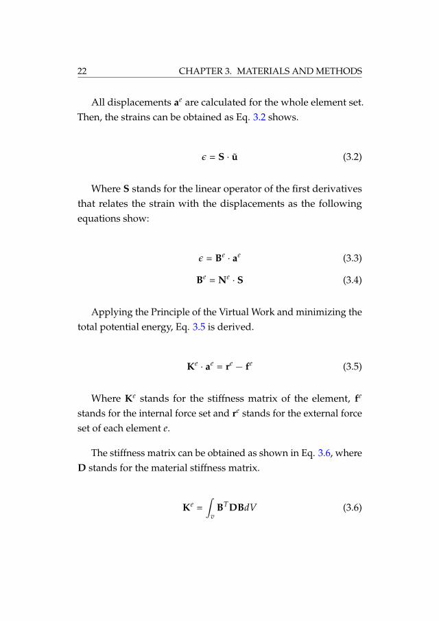
All displacements ae are calculated for the whole element set.Then, the strains can be obtained as Eq. 3.2 shows.
ε = S · u (3.2)
Where S stands for the linear operator of the first derivativesthat relates the strain with the displacements as the followingequations show:
ε = Be · ae (3.3)
Be = Ne · S (3.4)
Applying the Principle of the Virtual Work and minimizing thetotal potential energy, Eq. 3.5 is derived.
Ke · ae = re − fe (3.5)
Where Ke stands for the stiffness matrix of the element, fe
stands for the internal force set and re stands for the external forceset of each element e.
The stiffness matrix can be obtained as shown in Eq. 3.6, whereD stands for the material stiffness matrix.
Ke =∫
vBTDBdV (3.6)

3.1. BIOMECHANICAL MODELING OF SOFT TISSUE 23
The solution is obtained solving the system of equations de-fined in Eq. 3.7.
ri =
(m
∑e=1
Kei1
)· a1 +
(m
∑e=1
Kei2
)· a2 + · · · +
m
∑e=1
fei (3.7)
3.1.2 Hyperelasticity
Biological tissues are often considered as hyperelastic incom-pressible materials. These materials have a rubber-like behaviorand they present a stress-strain relationship that is non-linear,isotropic and incompressible. In this research, it was assumed thatthe breast and the cornea present this type of behavior.
Given a solid subjected to a displacement field ui(xk), eachelement of the deformation gradient tensor is defined as follows:
Fij = δij +∂ui
∂xj(3.8)
Where δij = 1 if i = j, and δij = 0 if i 6= j.
Having the strain energy density a function of the Left Cauchy-Green deformation tensor (Eq. 3.9) assures the isotropy of theconstitutive equation.
B = F · FT (3.9)
From the three eigenvalues of B: e1, e2 and e3, the principal

24 CHAPTER 3. MATERIALS AND METHODS
stretch directions are defined as follows:
λ1 =√
e1
λ2 =√
e2 (3.10)
λ3 =√
e3
Considering B as the deformation measure, the stress-strainenergy function W(F) can be written based on the invariants of B(Eq. 3.11).
I1 = trace(B) = λ21 + λ2
2 + λ23
I2 =12
(I21 − B2) = λ2
1λ22 + λ2
2λ23 + λ2
3λ21 (3.11)
I3 = det(B) = J2 = det(F)2 = λ21λ2
2λ23
J = det(F)
W(F) = ψ(I1, I2, I3, J) (3.12)
In this work, three different hyperelastic models were used: aneo-Hookean model, a Mooney-Rivlin model of second order, andan Ogden model.
Neo-Hookean model
The stress-strain function for the neo-Hookean model is de-fined by Eq. 3.13 [Treloar, 1948]. Where ψ stands for the strain

3.1. BIOMECHANICAL MODELING OF SOFT TISSUE 25
energy potential, I1 stands for the first invariant, J stands for thedeterminant of the deformation gradient tensor, µ stands for theinitial shear modulus of the material, and d stands for the materialincompressibility parameter.
ψ =µ
2(I1 − 3) +
1d
(J − 1)2 (3.13)
Mooney-Rivlin model
The constitutive equation of the Mooney-Rivlin model forsecond-order is given by Eq. 3.14 [Mooney, 1940; Rivlin, 1948].Where C1 and C2 stand for the material elastic parameters, K1
stands for the Bulk modulus, I1 and I2 stand for the first and sec-ond deviatoric strain invariants, and J stands for the determinantof the deformation gradient tensor.
ψ = C1(I1 − 3) + C2(I2 − 3) +K1
2(J − 1)2 (3.14)
Ogden model
The definition of the energy potential function of the N-orderOgden model is given by Eq. 3.15 [Ogden, 1972]. Where N standsfor the order, µi and αi stand for the elastic parameters, λi standfor the three deviatoric stretches defined in Eq. 3.11, K1 stands forthe initial Bulk modulus, and J stands for the determinant of theelastic deformation gradient.

26 CHAPTER 3. MATERIALS AND METHODS
ψ =N
∑i=1
µi
αi(λαi
1 + λαi2 + λαi
3 − 3) +K1
2(J − 1)2 (3.15)
3.2 Optimization by genetic heuristics
The search of the elastic constants of the constitutive modelsproposed to characterize the mechanical behavior of the breast andthe cornea was carried out by means of a parameter optimizationalgorithm driven by genetic heuristics.
Iterative search algorithms are often used to optimize a fitfunction f (X) with an unknown shape by changing the inputparameters X and using the output to minimize (or maximize) itsvalue.
X = arg min f (X) where X = {x1, x2, · · · , xn} (3.16)
Since the fit function can present multiple minima, search al-gorithms such as gradient descent may get stuck in one of thoseminima thus being unable to provide the best solution. This prob-lem can be avoided by running the algorithm multiple times withrandom initializations. Nevertheless, there are more effectiveapproaches for the global optimization like meta-heuristics.
One of the most known meta-heuristics is the evolutionary com-putation [Fogel, 1995; Jong, 2006]. Inspired in biological evolution,this type of heuristic drives the search by using the candidatesolutions to generate a new population iteratively. Evolutionaryheuristics have been already used to characterize mass-spring

3.2. OPTIMIZATION BY GENETIC HEURISTICS 27
models successfully [Bianchi et al., 2004; Xu et al., 2009]. Geneticalgorithms, a widely used meta-heuristic, was selected to drivethe methodology to estimate the elastic parameters of the biome-chanical models of the breast and cornea.
A Genetic Algorithm (GA) is a heuristic based on evolutionarycomputation used for optimizing problems [Chatterjee et al., 1996].This heuristic allows the reduction of the computational cost ofthe parameter optimization since it focuses on the most promisingareas while trying to explore the rest of the search space. A geneticalgorithm handles a population of individual solutions (parents)to a given problem and drives the evolution of the subsequentsteps of the search generating new candidate solutions (children).The population is modified by changing the individuals step bystep, this evolution leads to the optimal solution of the problem.Genetic algorithms are prepared to work on complex optimizationproblems where the fit function can present multiple minima.
3.2.1 Genetic operators
In each iteration of the GA, a new set of candidate solutions isgenerated by three generation formulas:
Selection: the best individuals (parents) are selected and usedto breed the next population.
Crossover: a combination of two parents forms a child.
Mutation: parents are randomly modified to form a child.

28 CHAPTER 3. MATERIALS AND METHODS
The successive populations of the iterative search are createdusing these three genetic operators. Since only the best individualsare considered as parents, the average fit function value is equal orbetter in each iteration while the search interval becomes smaller,thus reducing the search space in each iteration.
The GAs control the proportion of children generated whetherby selection, mutation or crossover with parameters which shouldbe adjusted for each optimization problem in order to get the bestresults.
3.2.2 GA outline
The GA works following this outline:
1. Initialize: a random population of samples X0 is created. It iscommon to set an interval for each parameter to be found inorder to help the algorithm to search in the area where theglobal minimum of the function may be located.
2. New population generation: iteratively, the algorithm creates anew candidate set of parameters Xi by means of the followingsteps:
a) The algorithm computes the fit function f (x) for each indi-vidual in the current set Xi.
b) Those individuals (called parents) with the best scores areselected.
c) Parents with the best score are tagged as elite and pass

3.2. OPTIMIZATION BY GENETIC HEURISTICS 29
Figure 3.1: Flowchart of the genetic algorithm
directly to the next population.
d) Parents are used to generate new children both by mutation(randomly changing a parent) and by crossover (combina-tion of several parents).
e) A candidate population Xi+1 is created by joining elites andchildren.
3. Termination: step 2 is repeated until a stop condition is reached.This can be a specific number of generations, a timer, or whenthe function does not change within a tolerance range. The setof parameters that minimized the function will be designatedas X.

30 CHAPTER 3. MATERIALS AND METHODS
A flowchart of the the genetic algorithm is shown in Figure3.1.
3.3 Similarity coefficients
In Biomechanics there are several methods used to compareand/or validate the proposed biomechanical models in order toknow their similarity regarding the real behavior of the organ.The work presented in [Crum et al., 2005] provides the accuracyof each registration method using the distance between fiduciallandmarks attached to a real organ. On the other hand, the volumedifference is also a measure that may provide information aboutthe fit goodness of a biomechanical model and it was used in [Shiet al., 2008]. However, the comparison using fiducial landmarksentails comparing only specific points on the surface and does notconsider the whole structure, ignoring the internal tissue distribu-tion. The same problem has the volume difference which is not avalid measure since it is not able to distinguish situations in whichthe organ is in different positions or the volume do not change.
A similarity measure commonly used in medical imaging forvalidating biomechanical models is the Normalized Mutual Infor-mation (NMI) [Studholme et al., 1999]. Using this type of image-based comparison may result in inaccurate results since NMI doesnot consider the spatial distribution of the tissues but only the grayvalue entropy of both 3D images. In [Lee et al., 2010] a Fourier-based correlation technique was used to compare the accuracyof the deformed breast compression model. In this case, as theauthors state, the technique only allows the comparison of images

3.3. SIMILARITY COEFFICIENTS 31
from the same modality and it does not take into account anyspatial information for the comparison.
In the recent literature, the similarity coefficients traditionallyused in validation of segmentation techniques have started to beapplied in the field of the computational biomechanics. Jaccardand Dice coefficients were used in [Balocco et al., 2010] to measurethe goodness of a registration algorithm using the biomechanicalproperties in cerebral aneurysms and Hausdorff coefficient wasused in [Vigneron et al., 2010] to validate a registration techniquethat uses a biomechanical model to simulate the deformationsuffered by the brain immediately after opening the skull. Unfor-tunately, the use of only overlap-based coefficients (like Jaccardor Dice) does not provide information about the shape of the vol-ume and using only distance-based coefficients (like Hausdorff)ignores the overlapped region.
The following section presents a study about how to applysimilarity coefficients traditionally used for validation of segmen-tation techniques in order to assess the error committed betweenthe simulation of the behavior of an organ and its real behavior.
3.3.1 Overlap and distance coefficients
The similarity coefficients usually operate over a 3D volume,thus abstracting all the processes from the number and type of ele-ments of a mesh (tetrahedron, hexahedron...). In order to comparetwo finite element meshes, they must be first converted to a 3Dvolume, this process is called voxelization. Methods for validationof segmentations techniques are easily applicable to volume com-
32 CHAPTER 3. MATERIALS AND METHODS
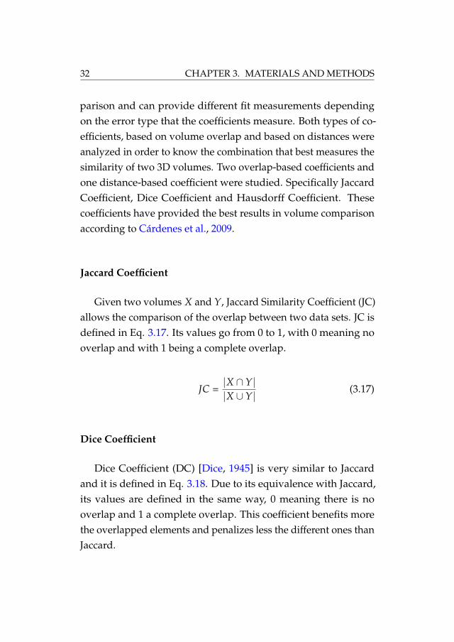
parison and can provide different fit measurements dependingon the error type that the coefficients measure. Both types of co-efficients, based on volume overlap and based on distances wereanalyzed in order to know the combination that best measures thesimilarity of two 3D volumes. Two overlap-based coefficients andone distance-based coefficient were studied. Specifically JaccardCoefficient, Dice Coefficient and Hausdorff Coefficient. Thesecoefficients have provided the best results in volume comparisonaccording to Cárdenes et al., 2009.
Jaccard Coefficient
Given two volumes X and Y, Jaccard Similarity Coefficient (JC)allows the comparison of the overlap between two data sets. JC isdefined in Eq. 3.17. Its values go from 0 to 1, with 0 meaning nooverlap and with 1 being a complete overlap.
JC =|X ∩Y||X ∪Y| (3.17)
Dice Coefficient
Dice Coefficient (DC) [Dice, 1945] is very similar to Jaccardand it is defined in Eq. 3.18. Due to its equivalence with Jaccard,its values are defined in the same way, 0 meaning there is nooverlap and 1 a complete overlap. This coefficient benefits morethe overlapped elements and penalizes less the different ones thanJaccard.

3.3. SIMILARITY COEFFICIENTS 33
DC =2|X ∩Y||X|+|Y| =
2JCJC + 1
(3.18)
Hausdorff Coefficient
The Hausdorff Coefficient (H) was introduced by Hausdorff in1962. This distance has been used in image comparison [Aspertet al., 2002; Lockett and Guenov, 2008; Vigneron et al., 2010] andits calculation has been improved to be applicable to big volumes[Huttenlocher et al., 1993].
Let’s define the distance dV(i) as the distance of the voxel ito the closest voxel of a volume V. If i ∈ V, then dV(i) is zero.The comparison was performed between two volumes X and Y,corresponding to the simulation and real behavior of the tissue,respectively. For the calculation of dX and dY, the euclidean dis-tance transform (EDT) was used [Ragnemalm, 1993]. The EDTallows the obtainment of all the distances in a matrix. Hence, theextraction of any dV(i) is immediate.
The Hausdorff Coefficient (Eq. 3.19) uses this distance to pro-vide a similarity value between two sets. It is defined as themaximum of the minimum distances between all the voxels of thevolume X to all the voxels of the volume Y and viceversa.
H(X, Y) = max∀i
(dX(i), dY(i)) (3.19)
In order to perform a complete evaluation of the right fitbetween volumes, both overlap-based coefficients and distance-

34 CHAPTER 3. MATERIALS AND METHODS
a) b)
Figure 3.2: Comparison of two different segmentations of an object a) and b),which provide similar value of the overlap-based coefficients.
based coefficients must be considered together. Figure 3.2 showsan example in which JC or DC would provide a similar value forthe comparison of both cases a) and b). Nevertheless, a) wouldbe an admissible deformation and b) would not. Therefore, addi-tional information can be used to distinguish these cases using,for instance, distance-based coefficients. Additionally, the sameproblem arises with distance-based coefficients, they may providesimilar values in very different cases. As Figure 3.3 shows, themaximum distance present in both a) and b) is the same and theHausdorff coefficient would provide similar values. Therefore,it could be difficult to differentiate these deformations withoutusing, for instance, overlap-based coefficients.
3.3.2 Analyzing the performance of the coefficients
The purpose of this study was to know which are the mostdiscriminant coefficients to compare the similarity of two vol-umes [Lago et al., 2012a]. In the case of the overlap-based coef-ficients, Jaccard and Dice coefficients were analyzed. Regardingthe distance-based coefficients, twenty four modifications of theHausdorff Coefficient were studied in order to create a large set ofmeasures to be studied. The 24 modifications corresponded to the

3.3. SIMILARITY COEFFICIENTS 35
a) b)
Figure 3.3: Comparison of two different segmentations of an object a) and b),which provide similar value of the original Hausdorff coefficient.
coefficients presented in [Dubuisson and Jain, 1994] and definedwith the direct distances shown in Eq. 3.20 to 3.25.
d1(X, Y) = minx∈X
(dY(x)) (3.20)
d2(X, Y) = K50thx∈XdY(x) (3.21)
d3(X, Y) = K75thx∈XdY(x) (3.22)
d4(X, Y) = K90thx∈XdY(x) (3.23)
d5(X, Y) = maxx∈X
(dY(x)) (3.24)
d6(X, Y) =1
NX∑
x∈XdY(x) (3.25)
Where KPthx∈X represents the Pth percentile of all the sorted dis-
tances and NX stands for the number of elements of the set X.Combining these distances with the combinations shown in Eq.3.26 to Eq. 3.29, the whole set of modified Hausdorff metrics is

36 CHAPTER 3. MATERIALS AND METHODS
constructed.
f1(X, Y) = min (di(X, Y), di(Y, X)) (3.26)
f2(X, Y) = max (di(X, Y), di(Y, X)) (3.27)
f3(X, Y) =di(X, Y) + di(Y, X)
2(3.28)
f4(X, Y) =NXdi(X, Y) + NYdi(Y, X)
NX + NY(3.29)
f1 f2 f3 f4
d1 D1 D2 D3 D4d2 D5 D6 D7 D8d3 D9 D10 D11 D12d4 D13 D14 D15 D16d5 D17 D18 D19 D20d6 D21 D22 D23 D24
Table 3.1: The 24 modified Hausdorff distances
Therefore, the direct distances di are combined with the f j
equations obtaining a set of 24 modified Hausdorff Coefficients(Table 3.1). It is noticeable that D18 corresponds to the originalHausdorff distance defined in Eq. 3.19. The distances from D1 toD4 were discarded because of their constant value throughout theproblem domain, thus leaving 20 Hausdorff modifications.
In addition to the modifications of the Hausdorff distance and,by taking advantage of the distance calculation, the distance ofthe surface voxels of a volume X to the nearest voxel of a vol-ume Y (and viceversa) were taken into account. The average of

3.3. SIMILARITY COEFFICIENTS 37
these distances (corresponding to d6(X, Y) and d6(Y, X)) and theirstandard deviations were also used for the analysis of the volumecomparison. These values are indicators of the homogeneity of thedistances between the surfaces of the volumes. Additionally, thesigned mean (Eq. 3.30) was added to the set of coefficients to bestudied since it could indicate the deviation of one volume withregard to the other one and viceversa.
SM = d6(X, Y)− d6(Y, X) (3.30)
Experimental set-up
Let’s summarize the 28 coefficients that were analyzed to selectthe best set to compare a simulated deformation of an organ tothe real one: two coefficients based on overlap (Jaccard and Dicecoefficients), the widely used volume difference (∆V), the 20 mod-ified Hausdorff coefficients (D5 to D24), the signed mean (SM),and the means and standard deviations of the distances betweenboth volumes (meandX , meandY , stddX , stddY ).
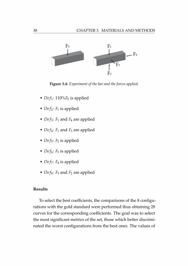
The experiment designed for the selection of the best metricswas a cantilevered bar (Figure 3.4) on which a force F0 was appliedto construct the gold standard deformation. A comparison be-tween the gold deformation caused by F0 and other 8 different de-formations (referred to as incorrect deformations) was performed.The 8 configurations combine forces in different directions andintensities as follows (F1 = F2 = F3 = F4 = 120%F0):
38 CHAPTER 3. MATERIALS AND METHODS
F1
F3
F2
F4
F0
Figure 3.4: Experiment of the bar and the forces applied.
De f1: 110%F0 is applied
De f2: F1 is applied
De f3: F1 and F4 are applied
De f4: F1 and F3 are applied
De f5: F2 is applied
De f6: F3 is applied
De f7: F4 is applied
De f8: F3 and F2 are applied
Results
To select the best coefficients, the comparisons of the 8 configu-rations with the gold standard were performed thus obtaining 28curves for the corresponding coefficients. The goal was to selectthe most significant metrics of the set, those which better discrimi-nated the worst configurations from the best ones. The values of

3.3. SIMILARITY COEFFICIENTS 39
the coefficients obtained in the comparison of these simulationsare shown in Figure 3.5. It can be considered the deformationsfrom best to worst (1 to 8). The values were normalized to be easilycompared and divided in six plots to allow for a better legibility.
From all the modifications of the Hausdorff coefficient, thosewhose De f5, De f6, and De f7 configurations did not show the worstvalues were rejected since these deformations must be consideredthe least similar to the gold deformation. The remaining Haus-dorff modifications were still valid. However, the D22 Hausdorffmodification, named as modified Hausdorff distance (MHD), wasselected since, according to [Dubuisson and Jain, 1994], its valuesincrease monotonically with the amount of difference, and is bet-ter at evaluating volume matching than the other distances thushaving more discriminatory power. Furthermore, it can be consid-ered that, in this experiment, neither the volume increment northe signed mean were useful to differentiate a good adjustmentfrom a bad one, therefore they were rejected.
Regarding overlap-based coefficients, both Jaccard and Diceshowed a similar behavior. Therefore, a different experimentfor the selection of the best overlap-based coefficient to performvolume comparisons was performed. A cylinder was comparedwith another one, of the same size and shape, but rotated on itsown axis. The union of both volumes with two different rotationsis shown in Figure 3.6.
The values obtained in this experiment are shown in Figure 3.7.Jaccard and Dice coefficients represented the level of overlappingbetween the two cylinders, giving the lowest value at the middle

40 CHAPTER 3. MATERIALS AND METHODS
1
2
3
4
5
6
7
8
-2 -1.5 -1 -0.5 0 0.5 1 1.5 2
con�
gura
tion
D 5D 6D 7D 8D 9
1
2
3
4
5
6
7
8
-2 -1.5 -1 -0.5 0 0.5 1 1.5 2
con�
gura
tion
D 10D 11D 12D 13D 14
1
2
3
4
5
6
7
8
-2 -1.5 -1 -0.5 0 0.5 1 1.5 2
con�
gura
tion
D 15D 16D 17D 18D 19
1
2
3
4
5
6
7
8
-2 -1.5 -1 -0.5 0 0.5 1 1.5 2
con�
gura
tion
D 20D 21D 22D 23D 24
1
2
3
4
5
6
7
8
-2 -1.5 -1 -0.5 0 0.5 1 1.5 2
con�
gura
tion
Mean V1Mean V2
StdV1StdV2
1
2
3
4
5
6
7
8
-2 -1.5 -1 -0.5 0 0.5 1 1.5 2
ΔV SM
JCDC
Figure 3.5: Values of all the metrics for the 8 configurations of the bar.

3.3. SIMILARITY COEFFICIENTS 41
Figure 3.6: Volume comparison of a rotated cylinder with respect to another.
of the curve (90◦). This curve also shows how Dice discriminatedless than Jaccard because of the lower decay of the Dice coefficientcurve compared with the decay of Jaccard coefficient one. There-fore, Jaccard was selected as the best overlap-based coefficient totake into account.
3.3.3 Geometric Similarity Function
The previous study showed that Jaccard coefficient (JC) andthe modified Hausdorff distance (MHD) were suitable coefficientsto compare the simulated deformation of an organ to the realone since they provide more information about the fit than theclassic comparison methods as volume difference or positions ofmarkers. They show how the error (or the lack of it) is distributedthroughout all the volume and provide information about theshape difference. However, as it was stated before, using only anoverlap-based measure or a distance-based coefficient does notprovide enough information to know whether two volumes aresimilar or not. Therefore, it is necessary a combination of both
42 CHAPTER 3. MATERIALS AND METHODS
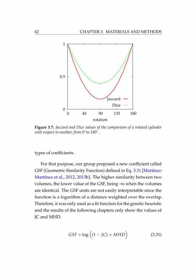
Figure 3.7: Jaccard and Dice values of the comparison of a rotated cylinderwith respect to another, from 0◦to 180◦.
types of coefficients.
For that purpose, our group proposed a new coefficient calledGSF (Geometric Similarity Function) defined in Eq. 3.31 [Martínez-Martínez et al., 2012, 2013b]. The higher similarity between twovolumes, the lower value of the GSF, being -∞ when the volumesare identical. The GSF units are not easily interpretable since thefunction is a logarithm of a distance weighted over the overlap.Therefore, it was only used as a fit function for the genetic heuristicand the results of the following chapters only show the values ofJC and MHD.
GSF = log(
(1− JC)×MHD)
(3.31)

3.3. SIMILARITY COEFFICIENTS 43
Figure 3.8: GSF values of the comparison of a rotated cylinder with respect toanother, from 0◦to 180◦.
The use of both parameters in the Geometric Similarity Func-tion combines the benefits of the overlap and the distance measure.It should be emphasized that, these coefficients can be used incombination with traditional biomechanical information as, forexample, strain-stress curves, or force-displacement curves, if theywere available.
Figure 3.8 shows the GSF values for the same rotating cylinderfrom the previous experiment. It is noticeable the high decay of thevalues when the similarity of the cylinders increases (angle near 0and near 180). This is a great indicator of the high sensitivity of theGSF with regard to small differences between volumes. For thisreason, the GSF is appropriate for the validation of biomechanicalmodels and as a fit function for the genetic algorithm.

44 CHAPTER 3. MATERIALS AND METHODS
3.4 Conclusions
This chapter has detailed the materials and methods used todevelop the methodology reported in this thesis. The theoreticalbase of the biomechanical models that were used to characterizethe behavior of the organs was established, focusing on the se-lected hyperelastic models that model the biomechanical behaviorof the breast and the cornea tissues.
Genetic heuristics have also been presented as the basis of theiterative search algorithm implemented to estimate the elasticconstants of the models in complex domains.
Finally, a study to select which coefficients are the best to com-pare two volumes has also been reported. These coefficients al-lowed the definition of the fit function to be used by the geneticheuristic. This function, the Geometric Similarity Function, con-siders the information of two types of similarity coefficients: anoverlap-based (Jaccard coefficient) and a distance-based (modi-fied Hausdorff distance), and is the core of the iterative search ofparameters.

Chapter 4
Characterization of thebiomechanical behavior ofthe breast
As mentioned in previous chapters, the accuracy of a patient-specific biomechanical model of the breast is a major concernfor applications such as surgical simulation, surgical guidance orcancer diagnosis. However, the elastic constants that define thebiomechanical behavior of the breast tissues are highly variableamong patients and their estimation becomes a very difficult task.
This chapter describes a methodology based on the simulationof the mammographic compression during an MRI-guided biopsyfor the in-vivo characterization of the biomechanical behavior ofthe breast. An iterative search algorithm is used to find the elastic
45

46 CHAPTER 4. CHARACTERIZATION OF THE BREAST
constants of the constitutive equations of the model proposed tocharacterize the three main tissues of the breast: fat, glandulartissue and skin. The methodology was applied for the character-ization of breast software phantoms [Pokrajac et al., 2012]. Thebiomechanical model chosen to characterize the breast tissues wasthe anisotropic neo-Hookean hyperelastic model proposed by Hanet al., 2012. Results from this analysis showed that following theproposed methodology, the elastic properties of each tissue wereestimated with a mean relative error of about 10% [Lago et al.,2014a].
4.1 Breast anatomy
The female breast is a glandular organ formed by differentinternal structures, namely: adipose tissue, fibroglandular tissue,Cooper’s ligaments, the ductal network and, finally, a complexmixture of smaller structures like blood vessels, nerves and lym-phatics.
The fibroglandular tissue region has a conical form extendingfrom the nipple to the chest wall. This cone is called the parenchy-mal cone and it is surrounded by adipose tissue which allowsthe mobility on the chest wall [Egan, 1988]. The adipose tissueregion is formed by different adipose compartments separated bythe Cooper’s ligaments. Those suspensory ligaments are fibrousstructures connected to the skin that provides structural supportto the breast. The ductal network is formed by ducts starting inthe glandular secretory lobes (or gland lobules) and ending in thenipple, the ducts are surrounded by glandular tissue. An average

4.2. BREAST IMAGING SYSTEMS 47
Figure 4.1: Mammary gland (anterolateral dissection) [Netter, 1989]
adult breast contains 15-20 lobes each one of them has its ownmajor duct [Lamarque, 1984]. The breast is attached to the pectoralmuscle, which connects it to the chest wall between the 2nd andthe 6th ribs. The breast is wrapped by the skin, a combination ofcutaneous and subcutaneous layers with a thickness between 0.5mm and 3 mm [Ulger et al., 2003; Gefen and Dilmoney, 2007]. Fig-ures 4.1 and 4.2 show a section of the female breast in anterolateralan sagittal directions respectively [Netter, 1989].
4.2 Breast imaging systems
Early detection of cancer is of great importance since an earlytreatment may be crucial for the patient. X-ray mammography is

48 CHAPTER 4. CHARACTERIZATION OF THE BREAST
Figure 4.2: Mammary gland (sagittal section) [Netter, 1989]

4.2. BREAST IMAGING SYSTEMS 49
the most common imaging modality for breast cancer diagnosis[Schulz-Wendtland et al., 2009] but there are some other commonexploration techniques such as magnetic resonance images (MRI)or tomosynthesis.
4.2.1 X-ray Mammography
X-rays were discovered in 1895 by Wilhem Conrad Roentgenthus being the oldest non-invasive technique of body imaging. AnX-ray is an electro-magnetic radiation that is able to traverse thehuman body. The thickness and density of human tissues affectthe magnitude of absorption of X-rays introducing a differencein the X-ray beam past the patient that is captured by a detector.The denser the tissue, the more X-rays it absorbs [Johns and Yaffe,1987].
The generation of the X-rays is performed by accelerating anelectron beam in a vacuum tube directing it towards the anode.The deceleration of the electrons produces electromagnetic energy(X-ray photons) which traverses the material in their path. Indigital mammography, the X-rays fall upon a special detectorwhich transforms the X-rays into electrical signals. These signalsare used to produce images of the breast and sent to a computerfor further processing.
The absorption of the X-rays causes the ionization of the tra-versed tissues thus needing a strict control of the dose receivedby the patient. For that purpose, a filter is placed between thegenerator and the patient in order to control the power of the X-ray.Specifically, for mammography imaging the X-ray energy needed

50 CHAPTER 4. CHARACTERIZATION OF THE BREAST
is low [Curry et al., 1990]. However, the area around the nipplemay be overexposed to the X-rays while the region nearest to thechest wall may be underexposed causing a low-quality image. Toavoid this problem, the breast is placed between two plates thatcompress it up to a 50% of its original size thus balancing thethickness of the breast in the X-ray direction as well as spreadingthe tissues in a larger surface reducing the possible overlap of in-teresting regions. The amount of compression is not a fixed valueand it may vary between patients and acquiring sessions. Thereare two typical compression types: cranio-caudal (CC) compres-sion, in which the plates are placed horizontally, and mediolateraloblique (MLO) compression, in which the plates are rotated up to70◦. Figure 4.3 shows the mammography device and an exampleof both MLO and CC mammograms of the same breast.
4.2.2 Magnetic Resonance
In magnetic resonance (MR) devices, a magnetic field is ap-plied on the breast thus changing the magnetic equilibrium of thetissues and then, a radiofrequency pulse disturbs the magnetiza-tion. The tissues are bound to recover their initial magnetism thusemiting electromagnetic waves towards an antenna that detectsthis variation and generates a 2D image [Hesselink, 2006]. Thistype of wave is completely innocuous for the patient and it is ableto traverse the bones without energy loss. This process is repeatedin several 2D slices and the result is a 3D image of the studiedregion.
Breast MRI is usually performed in different configurationswhich can attenuate certain tissues. Both T1 configuration (fat sup-

4.2. BREAST IMAGING SYSTEMS 51
Figure 4.3: Top: Mammography device used in CC position. Bottom Left:MLO X-ray mammogram. Bottom Right: CC X-ray mammogram

52 CHAPTER 4. CHARACTERIZATION OF THE BREAST
Figure 4.4: MRI slice of the chest in two different configurations T1 (left) andT2 (right)
pression) and T2 configuration of a breast MR image are shown inFigure 4.4. This modality is less common than X-ray mammogra-phy and it is used as an alternative imaging technique when thereare suspicious areas that are not successfully distinguished in theX-ray mammography.
The MRI can also be used for breast guided biopsy. This isuseful when the lesion cannot be detected in the X-ray mammog-raphy or by ultrasound. The patient lays in prone position in theMRI scanner as Figure 4.5 shows. The breast is placed betweentwo plates which compress it to avoid displacements that cancause maladjustments during the biopsy. The scanner takes MRimages in between the moments when the clinician operates witha needle, trying to reach the lesion. The procedure ends when asample of the lesion is retrieved and a little marker is placed in thebiopsy site. This marker is used to localize the lesion afterwardsfor future treatments.

4.3. SOFTWARE BREAST PHANTOMS 53
Figure 4.5: MRI biopsy device. © Mayo Foundation for Medical Educationand Research.
4.3 Software breast phantoms
Virtual clinical trials (VCTs) whose images can be generatedusing software phantoms represent an important pre-clinical alter-native for validating imaging systems in different modalities. Soft-ware phantoms can be used to create large data-sets of syntheticimages with known ground truth about the simulated anatomy.They also offer flexibility to cover anatomical variations in theshape, size, and tissue distribution [Bakic et al., 2002].
Breast software phantoms, in particular, allow the creationof large sets of samples to simulate the images provided by thedifferent types of imaging systems commonly used in breast can-cer diagnosis: X-ray mammography, magnetic resonance (MR),or computerized tomography (CT) [Bakic et al., 2011]. Software

54 CHAPTER 4. CHARACTERIZATION OF THE BREAST
phantoms can be applied to know the feasibility of a wide rangeof studies as: simulation of multimodality imaging systems [Diek-mann et al., 2009; Bakic et al., 2011; Chen et al., 2011; Chui et al.,2012], evaluation of breast dosimetry [Dance et al., 2005; Zhouet al., 2006; Ma et al., 2009; Sechopoulos et al., 2012], or evaluationof registration techniques [Richard et al., 2006].
Realistic virtual breast phantom development has been stud-ied since early 2000’s. Early development of 3D virtual breastphantoms was presented by [Bliznakova et al., 2003, 2010]. Thisphantom uses a combination of 3D geometrical primitives andvoxel matrices including not only the Cooper’s ligaments, skinand pectoral muscle but also the duct system and lobular units(Figure 4.6). This method generates a phantom which consists in a3D mammographic texture, combination of all the primitive ge-ometries in a voxelized 3D space. However, this type of phantomis only useful for mammographic simulations and simulation ofX-ray modalities.
Similarly, the phantom developed by [Chen et al., 2011] alsohas the ability for multimodality imaging simulation. In this case,the phantom is formed by a random generation of skin, fat tissue,glandular tissue and a network of ductal trees. A compressionmodel is applied and the compressed phantom is used to simulateimage modalities such as mammography, computer tomographyor tomosynthesis.
In [Li et al., 2009], the breast phantom is generated by meansof real breasts. The segmented data from a real breast CT is usedto create a model for the breast which is later compressed to sim-

4.3. SOFTWARE BREAST PHANTOMS 55
Figure 4.6: Phantom by Bliznakova et al.
ulate the mammography positioning (Figure 4.7). However, itsdependence on a real breast reduces its variability since it is tiedto the number of samples thus reducing the automaticity.
Recently, the work by [Bhatti and Sridhar-Keralapura, 2012]presented a complex 3D virtual breast phantom aimed to inves-tigate the biomechanics of the elastography (Figure 4.8). This phan-
Figure 4.7: Phantom by Li et al.

56 CHAPTER 4. CHARACTERIZATION OF THE BREAST
Figure 4.8: Phantom by Bhatti and Sridhar-Keralapura
tom is created by a mechanical design tool and can be parametrizedin tumor location, glandular density and ductal structure. Al-though being very realistic, this phantom needs a manual processto generate most of the geometry and it was not tested for largedeformations like mammographic compression.
The work by Bakic et al., 2002 presented a methodology forgenerating a computer breast model with realistic internal tissuedistribution, including fat tissue, glandular tissue, Cooper’s liga-ments, and skin (Figure 4.9). These phantoms have been used invarious clinical breast imaging modalities including digital mam-mography and digital breast tomosynthesis [Bakic et al., 2010;Vieira et al., 2013; Young et al., 2013], ultrasound tomography[Yang et al., 2012], and magnetic resonance [Nishikawa et al.,2011]. Later, they improved the model by using a region growing

4.3. SOFTWARE BREAST PHANTOMS 57
Figure 4.9: Phantom by Bakic et al., 2011
algorithm thus accelerating the generation process and enhanc-ing the realism of the internal tissue distribution [Bakic et al.,2011]. Finally, the phantom generation was also accelerated onthe Graphical Processing Unit (GPU) using octrees [Pokrajac et al.,2012; Chui et al., 2012]. This is the phantom that was used toprove the methodology due to the ability of the algorithm to gen-erate phantoms controlling the shape, size and fat/glandular ratioeasily. An example of this phantom is shown in Figure 4.10.

58 CHAPTER 4. CHARACTERIZATION OF THE BREAST
Figure 4.10: Left: coronal section of a raw phantom. Right: mediolateralsection of the corresponding phantom. Each gray level denotes each tissue type:white pixels correspond to the glandular tissue, light gray pixels correspond tothe fat tissue, dark gray lines correspond to the Cooper’s ligaments and mid-darkgray pixels surrounding the phantom correspond to the skin. [Pokrajac et al.,2012]
4.4 Study of the mesh quality
This study was motivated by the necessity of generating largedata-sets of synthetic X-ray mammograms for virtual clinical trials.
In order to get an accurate solution for the simulation of thecompression of the breast, the finite element method (FEM) arisesas the best method to predict the breast tissue distribution af-ter mammographic compression [Matthews and West, 1972; Ra-jagopal et al., 2006; Han et al., 2011; Lago et al., 2012b,c, 2013a].

4.4. STUDY OF THE MESH QUALITY 59
However, the iterative nature of this method is usually slow andbecomes a bottleneck in the pipeline of generation of virtual breastimages if adequate meshes are not used in the process. The simu-lation of the mammographic compression is the slowest step andthe quality of the finite element mesh constructed to perform thatsimulation is of great importance for the accuracy and efficiencyof this pipeline [Lago et al., 2013b].
Mesh quality should be an important issue to consider whendealing with realistic simulations of the biomechanical behaviorof the soft living tissues. Generation of FE meshes that accuratelyrepresent the geometry of organs as the breast is a well-knownproblem in soft tissue biomechanics. The quality of the FE meshesconstructed for these organs can affect the solution of simulationscarried out using the FEM since low quality meshes may lead tounrealistic results or may present convergence problems. How-ever, many works do not perform mesh quality analysis beforethe FE simulations [Bucki et al., 2011; Burkhart et al., 2013].
Patient-specific FE meshes that consider the different tissues ofthe breast can be automatically generated by commercial softwarepackages. However, these meshing software usually create irreg-ular meshes due to the complexity of the breast internal tissues[Tanner et al., 2006a; Kellner et al., 2007]. Automatic generation ofpatient-based finite element meshes considering the different tis-sues of the breast usually lead to bad quality elements (tetrahedrain this case), especially at the boundaries between the differenttissues. These regions are usually meshed with many elements,often irregular or distorted, in order to fit the boundary surfaces.A manual intervention for refining these regions is needed in or-

60 CHAPTER 4. CHARACTERIZATION OF THE BREAST
der to improve the mesh quality, for avoiding non-convergences,and for reducing the computational cost of the FEM [Bucki et al.,2011]. Being able to use regular meshes with good-quality ele-ments may reduce the time consumed by the FEM and the risk ofnon-convergence.
In this section, a comparison of the breast tissue distributionafter the simulation of the compression of an X-ray mammogra-phy by two different meshing approaches was detailed. A meshcreated with elements adapted to the distribution of the inter-nal tissues (adaptive mesh) and a mesh constructed with regularelements (homogeneous mesh) automatically generated by a com-mercial software were used for this study.
4.4.1 Materials and Methods
Synthetic generation of X-ray mammograms involves perform-ing three major tasks: generating a 3D software phantom, simulat-ing the mammographic compression, and projecting the deformedphantom to obtain a 2D virtual mammogram. The generationof the 3D breast anatomy of the phantom was carried out usingthe computer anthropomorphic breast phantoms developed atthe University of Pennsylvania (UPenn) described in Section 4.3[Bakic et al., 2002, 2011; Pokrajac et al., 2012].
Generation of the finite element mesh
Once the software phantom was generated, the next step wasto obtain the finite element mesh from the virtual geometry. Forthat, two approaches were considered:

4.4. STUDY OF THE MESH QUALITY 61
Adaptive mesh: constructing the mesh considering the differ-ent tissues of the breast.
Homogeneous mesh: constructing the mesh considering thewhole breast as a single tissue and assigning material prop-erties to the elements afterward.
In the first case, the meshing software draws the boundariesbetween tissues creating small elements on those regions andbigger elements on the areas with the same material. The resultis a large number of poor quality elements dedicated to draw theboundaries.
In the second case, the meshing software is blind to the breasttissues, thus creating a regular mesh of the whole breast as if itwas only made out of a single material. In this case, the meshingalgorithm is able to create elements with more regular shape andsize since it finds no restrictions due to the internal tissue distribu-tion. Regarding how this algorithm takes into account the tissuedistribution, the most prevalent material in an element is assignedto it afterward.
In both cases, the commercial software Simplewarer was usedto create meshes using tetrahedral elements. The skin and Coo-per’s ligaments were not meshed separately since these structuresare not clearly visible in some clinical modalities [Solves Llorenset al., 2012; Han et al., 2012]. Moreover, narrow structures likethe skin would require a large number of irregular elements inthe adaptive meshing. Therefore, for this study, the breast wasassumed to be formed by fat tissue, which included skin and
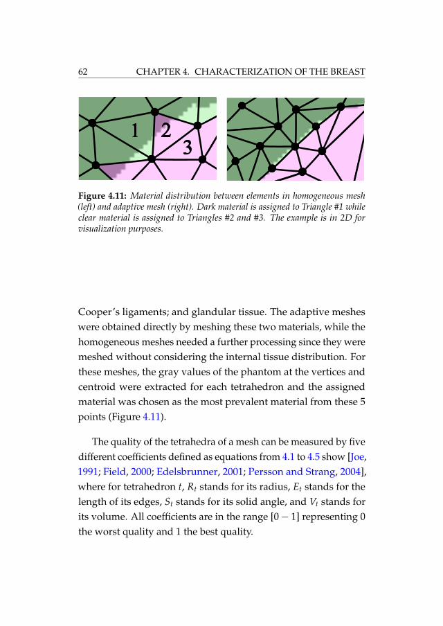
62 CHAPTER 4. CHARACTERIZATION OF THE BREAST
13
2
Figure 4.11: Material distribution between elements in homogeneous mesh(left) and adaptive mesh (right). Dark material is assigned to Triangle #1 whileclear material is assigned to Triangles #2 and #3. The example is in 2D forvisualization purposes.
Cooper’s ligaments; and glandular tissue. The adaptive mesheswere obtained directly by meshing these two materials, while thehomogeneous meshes needed a further processing since they weremeshed without considering the internal tissue distribution. Forthese meshes, the gray values of the phantom at the vertices andcentroid were extracted for each tetrahedron and the assignedmaterial was chosen as the most prevalent material from these 5points (Figure 4.11).
The quality of the tetrahedra of a mesh can be measured by fivedifferent coefficients defined as equations from 4.1 to 4.5 show [Joe,1991; Field, 2000; Edelsbrunner, 2001; Persson and Strang, 2004],where for tetrahedron t, Rt stands for its radius, Et stands for thelength of its edges, St stands for its solid angle, and Vt stands forits volume. All coefficients are in the range [0− 1] representing 0the worst quality and 1 the best quality.

4.4. STUDY OF THE MESH QUALITY 63
M1 = 3× Rinspheret
Rcircumspheret
(4.1)
M2 = 2√
6× Rinspheret
max Et(4.2)
M3 = 12× (3×Vt)2/3
∑61 E2
t(4.3)
M4 = min St (4.4)
M5 =min Vt
max Vt(4.5)
On the other hand, widely used FE software packages likeABAQUSr or ANSYSr usually perform a quality test on thefinite element mesh. These software packages show messagesof warning when the aspect ratio of a tetrahedron is not goodenough. The aspect ratio of a tetrahedron is defined as the ratiobetween the longest edge and the shortest normal from one vertexto the opposite face and it is related to the angles between faces. Aregular tetrahedron (Figure 4.12, left) has an aspect ratio of 1.
All these coefficients were taken into account to measure thequality of the constructed meshes.

64 CHAPTER 4. CHARACTERIZATION OF THE BREAST
Figure 4.12: Regular tetrahedron with a high aspect ratio (left) and anotherone with lower aspect ratio (right).
Table 4.1: Parameters used for the neo-Hookean model.
µ ν
fat 12 750 Pa 0.49glandular 36 750 Pa 0.49
4.4.2 Simulation of the mammographic compression
To perform this study, the neo-Hookean hyperelastic model de-scribed in Section 3.1.2 was chosen to simulate the deformation ofthe breast tissues in the compression during X-ray mammography.The parameters used for this model were taken from the literature[Gefen and Dilmoney, 2007] and are shown in Table 4.1.
The mesh of the breast phantom was placed between two rigidplates (Figure 4.13) and, as boundary conditions, the nodes be-longing to the chest wall were restricted in the chest wall-nippledirection. Additionally, the nodes already in contact with the fixedplate were restricted in all directions in order to avoid rigid bodymotion [Ruiter et al., 2006]. A sliding contact interaction withoutfriction was defined between the breast surface and both platesin order to facilitate the FE simulation. The reason was that thefriction coefficient between the breast and the plates is unknown[Shih et al., 2010]. Finally, a displacement was applied to the mo-bile plate in order to compress the breast up to 50% of its thickness
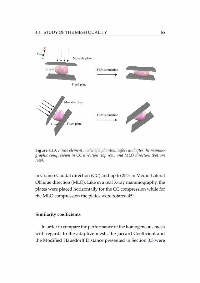
4.4. STUDY OF THE MESH QUALITY 65
Figure 4.13: Finite element model of a phantom before and after the mammo-graphic compression in CC direction (top row) and MLO direction (bottomrow).
in Craneo-Caudal direction (CC) and up to 25% in Medio-LateralOblique direction (MLO). Like in a real X-ray mammography, theplates were placed horizontally for the CC compression while forthe MLO compression the plates were rotated 45◦.
Similarity coefficients
In order to compare the performance of the homogeneous meshwith regards to the adaptive mesh, the Jaccard Coefficient andthe Modified Hausdorff Distance presented in Section 3.3 were

66 CHAPTER 4. CHARACTERIZATION OF THE BREAST
considered. Additionally, centroid distance and volume differencewere also computed since they provide a very intuitive value ofthe similarity between two compartments.
Generation of the compressed 3D phantom
Once the breast mesh was compressed, the deformed 3D phan-tom was obtained. The compressed phantom is the result of inter-polating the original 3D phantom as a texture. Each tetrahedron(before and after the deformation) was used to know how theoriginal phantom had to be deformed. The interior gray valuesof each tetrahedron before the deformation were interpolated toobtain the new position in the deformed tetrahedron, thus creatingthe new 3D texture. This step was run on the GPU in order toaccelerate the generation.
4.4.3 Results of the mesh quality analysis
Ten phantoms of ratio dense/fat tissue between 7% and 35%,250 ml of volume and identical shape, were generated. The size ofthe uncompressed phantoms was 170 mm in vertical direction, 100mm in lateral direction and 50 mm in chest wall-nipple direction.For each phantom, both the adaptive mesh and the homogeneousmesh were created using Simplewarer with the following charac-teristics:
Adaptive mesh: 5 mm as maximum edge length of the tetra-hedron and 0.5 mm as minimum.
Homogeneous mesh: the length of the tetrahedron edges was

4.4. STUDY OF THE MESH QUALITY 67
set to be 1 mm.
In addition, the quality of the tetrahedra of both meshes wasmaintained as high as possible by means of the parameters thatSimplewarer provides for that purpose. This way, the size of theadaptive meshes was in the order of 900 000 elements and 180 000nodes. On the other hand, the homogeneous meshes were formedby 425 000 elements and 90 000 nodes. The same homogeneousmesh was used for all the phantoms since the differences amongthe meshes only corresponded to the difference of the internaltissue assignation. Figure 4.14 shows the same slice of both theadaptive mesh and the homogeneous mesh for the same phantom.The smoothness in the boundaries between dense and fatty tissueis noticeable for the adaptive mesh while the homogeneous meshshows a sharper contour. However, the homogeneous mesh showsmore regular elements and, therefore, elements of higher quality.On the other hand, the adaptive mesh presents more distortedand lower quality elements, especially in the boundaries betweentissues.
In order to make comparable the results obtained for eachdeformed phantom, both meshes, the adaptive mesh and thehomogeneous mesh, were constructed so that the mesh qualitycoefficients mentioned in Section 4.4.1 presented similar values forboth of them. This was possible for all the coefficients except forcoefficient M5. The reason is that M5 is related to the homogene-ity of the mesh, thus being impossible to achieve a similar valuefor both meshes since the elements of the adaptive meshes haddifferent sizes and shapes all over the volume. Figure 4.15 showsthe average values obtained by the aforementioned mesh quality

68 CHAPTER 4. CHARACTERIZATION OF THE BREAST
Figure 4.14: Slice of the adaptive mesh (top) and corresponding slice of thehomogeneous mesh (bottom) of the same phantom. Dark color represents theglandular tissue and clear color represents the fat tissue.
coefficients. The figure compares how the quality of the adaptivemesh is dependent of the minimum edge length of the elements,from 3 mm to 1 mm as well as the quality of the mesh without anyrestriction in the edge length (non-refined mesh). Furthermore, alltetrahedra of the constructed meshes had an average aspect ratiobelow 10. The reason was that a tetrahedron is considered as abad element if its aspect ratio is equal or greater than 10 [Hibbittand Sorensen, 2001]. This, along with the aforementioned meshquality coefficients, ensured enough quality in all meshes to makecomparable their performance in the simulation of the mammo-

4.4. STUDY OF THE MESH QUALITY 69
Figure 4.15: Value of the five quality measures for different mesh sizes includ-ing the non-refined adaptive mesh without any edge length restriction (firstbar), adaptive mesh with different minimum edge lengths (3 mm, 2 mm, and1 mm) and the homogeneous mesh (last bar). All the measures have a rangebetween 0 and 1, with 1 being the highest quality.
Table 4.2: Average and worst aspect ratios for the adaptive mesh and thehomogeneous mesh for all the phantoms.
average worstadaptive 1.70 8.86homogeneous 1.55 5.33
graphic compression due to an X-ray mammography. Table 4.2shows the average aspect ratio for both adaptive and homogenousmesh.
The simulation of the mammographic compression was per-formed using FEBio, an open source software for solving nonlinearfinite element equations in biomechanical applications [Maas et al.,2012]. The used computer was an Intel Xeon X5650 @ 2.66 GHz (12cores) with 64GB of RAM. The average time consumed by FEBioto solve every simulation using either the adaptive mesh and the

70 CHAPTER 4. CHARACTERIZATION OF THE BREAST
Figure 4.16: Average time needed to solve the deformation for every 1000elements and standard deviation.
homogeneous mesh was also measured. Figure 4.16 shows theaverage time required to obtain the deformation for every 1000elements in the CC direction.
The comparison of the deformed phantoms was carried outusing only the dense tissue compartments. The large number offat compartments could cause the average values to be less signifi-cant. Moreover, the majority of the differences were present in theneighborhood of dense tissue compartments, hence, the focus wasmade on these areas. Table 4.3 shows the results of the comparisonof the deformed phantoms for both CC compression (top row)and MLO compression (bottom row), respectively. Values of thesimilarity coefficients reported in Section 3.3 are provided for bothsimulations in this table. Additionally, Figure 4.17 shows a visualcomparison of the same slice from a deformed phantom using anadaptive mesh and a homogeneous mesh.
Finally, the last step in the generation of phantom mammo-grams consists in the simulation of the X-ray projection through

4.4. STUDY OF THE MESH QUALITY 71
Table 4.3: Comparison between the homogeneous mesh and the adaptive meshusing a neo-Hookean model for dense compartments in CC and MLO compres-sion for 10 phantoms.
cent. dist. vol. diff. JC MHDCC 2.54 vox 1759.4 vox 0.8257 1.1792 voxMLO 0.2683 vox 197.9 vox 0.8723 1.2772 vox
Figure 4.17: Corresponding slices of the same deformed raw phantom using anadaptive mesh (left), a homogeneous mesh (middle) and their absolute differences(right).
the deformed phantom. The projections were simulated usingthe ray tracing algorithm, assuming the ideal (point) focal spot,polyenergetic X-ray beam without scatter and an ideal detectormodel. The X-ray quantum noise and the electronic noise weresimulated by adding two Poisson distributed random processes.Figure 4.18 shows a projection of the same phantom deformedusing the adaptive mesh and the homogeneous mesh and theirsigned differences. The signed differences show dark and white

72 CHAPTER 4. CHARACTERIZATION OF THE BREAST
Figure 4.18: X-Ray mammographic projection of the same phantom usingadaptive mesh (left), homogeneous mesh (right) and their absolute differences(right). Gray pixels indicate equal values in the images while black and whitepixels indicate the differences.
values for differing pixels of the adaptive mesh and homogeneousmesh models respectively. Gray values correspond to identicalpixels.
4.4.4 Discussion
All similarity coefficients used to compare the adaptive meshesand the homogeneous meshes showed that the difference wasmostly in the size of the compartments (Table 4.3). Bearing in mindthat the phantom resolution was 200 µm, the average distancebetween compartment centroids was 0.508 mm (2.54 voxels) in theCC compression while in the MLO compression, the differencewas 0.05 mm (0.2683 voxels). On the other hand, the averagevolume difference was 14.08 mm3 (1759.4 voxels) and 1.58 mm3

4.4. STUDY OF THE MESH QUALITY 73
(197.9 voxels), respectively. Considering that the volume of theoriginal phantom is 250 000 mm3, these differences represent lessthan a 0.0065% of the total volume.
A value of Jaccard Coefficient of approximately 0.8 indicatesthat the overlap was not complete because of the small size ofsome compartments. In these cases, a displacement of a few vox-els could cause JC to move to low values. The JC values increasedquickly if these compartments were ignored. Nevertheless, MHDpresented very low values, approximately 0.24 mm (1.2 voxels)for CC and MLO compression. Taking into account that the com-pression was from 100 mm to 50 mm in CC and the voxel size was200 µm, differences of less than 1 mm between compartments canbe neglected. It is important to highlight that the values of thesimilarity coefficients were better in MLO compression than in CCcompression since the breast is subjected to a higher deformationin CC than in MLO.
In order to know how much influence the chosen biomechani-cal model had on the results, an identical study was performedusing the Mooney-Rivlin hyperelastic model proposed by [Tanneret al., 2006b]. In this case, results showed an average distancebetween compartment centroids comparing adaptive mesh versushomogeneous mesh of 0.66 mm in CC and 0.17 mm in MLO whilethe difference in volume was 16.3 mm3 in CC and 2.63 mm3 inMLO. The chosen model does not make any difference betweenboth meshing types since the Mooney-Rivlin model provided sim-ilar results to the neo-Hookean model. Both models have provedtheir suitability to simulate the mammographic compression forreal cases [Gefen and Dilmoney, 2007; del Palomar et al., 2008;
74 CHAPTER 4. CHARACTERIZATION OF THE BREAST
Rajagopal et al., 2008; Chung et al., 2008; Shih et al., 2010].
Regarding the time needed for the simulation of the mam-mographic compression, the homogeneous mesh presented muchfaster convergence than the adaptive mesh. For the adaptive mesh,the solution needed, on average, approximately 23 seconds per1000 elements and in the case of the homogeneous mesh, the timeneeded per 1000 elements was 15 seconds. Given that the elementsof the homogeneous mesh were more regular, their solving timeswere much shorter than the time needed to solve the problemusing the adaptive mesh. This was one of the main consequencesof having an irregular mesh, the time needed to get the solutionincreases with the number of bad-quality tetrahedra. The stan-dard deviation of the time points out the great impact that themesh quality had in the solver and, therefore, in the solution. Theaverage total time for deforming the adaptive meshes in CC di-rection was around 7 hours while for the homogeneous mesheswas around 2 hours, having both of them similar quality and pro-viding virtually identical results. For the MLO compression, theaverage total time was 2 hours for deforming the adaptive meshand 1.45 hours for the homogeneous mesh.
Even though one of the main advantages of the adaptive meshis to need less elements, the number of elements in the adaptivemesh after the refinement was much higher than the number ofelements in the homogeneous mesh. This was due to the difficultyof constructing an automatic adaptive mesh with good qualityelements, especially in the regions between tissues. Generatingthe adaptive mesh with less elements resulted in a considerablereduction of the quality of the tetrahedra thus providing an un-

4.4. STUDY OF THE MESH QUALITY 75
reliable solution when compared to the solution with the homo-geneous mesh. On the other hand, the unconstrained nature ofthe homogeneous mesh resulted in sharp boundaries between tis-sues. The homogeneous mesh is only an approximation to the realboundaries but this becomes a trade-off: increasing the number ofelements would make the elements of the mesh closer to the realtissue distribution but it would also increase the time needed tosolve the FEM.
Finally, figures 4.17 and 4.18 confirm that the differences be-tween the deformed phantom and its projection using the adaptivemesh and the homogeneous mesh are mostly in the surroundingsof the glandular compartments. The random noise added to theprojections is the responsible of the rough texture present in theprojection difference.
In summary, the homogeneous meshes are more adequate toperform the simulation of the mammographic compression fora pipeline of synthetic mammograms generation. The homoge-neous meshes provided the same degree of accuracy than theadaptive meshes independently of the model chosen to representthe biomechanical behavior of the breast tissues but with shortercomputational times [Lago et al., 2013b].
Using homogeneous meshes in an automatic pipeline of breastmammogram simulations can speed up the generation of sampleswithout losing accuracy since they do not need manual interven-tion to be repaired and polished. This may lead to a fast automaticpipeline of virtual mammogram generation starting with the phan-tom creation and ending with the simulated X-ray projection.

76 CHAPTER 4. CHARACTERIZATION OF THE BREAST
4.5 Biomechanical modeling of the breast tis-sues
There are many models proposed to simulate the breast tis-sue behavior. The most simplistic models considered the breastas a homogeneous tissue [Carter et al., 2008]. Roose et al., 2006used an elastic model to simulate the breast behavior, however,for large deformations, the soft tissue presents hyperelastic be-havior [Rajagopal et al., 2008]. The work in [Ruiter et al., 2006]compared different elastic and hyperelastic models in order tosimulate the mammographic compression, they concluded thatthe anisotropy of the breast due to the internal tissue distributionmust be considered for simulating this compression. Additionally,simplifying the breast model without considering the internal tis-sues may lead to unrealistic simulations and that approximationcould cause overestimation on the X-ray dose with the resultantoverestimation of the risk for the patient [Sechopoulos et al., 2012].
To accurately model the breast biomechanical behavior, theresponse of the three main internal tissues must be modeled: fat,glandular tissue and skin. For that reason, other works reportedheterogeneous models of the breast [Azar et al., 2001; Samani andPlewes, 2004; del Palomar et al., 2008; Pathmanathan et al., 2008;Solves Llorens et al., 2012].
On the other hand, even though most biomechanical models ofthe breast do not include the anisotropy of the Cooper’s ligamentsdue to the difficulty of knowing their location, some sensitivitystudies consider that their influence is significant [Tanner et al.,2006b; Ruiter et al., 2006; Gefen and Dilmoney, 2007]. Therefore,

4.5. BIOMECHANICAL MODELING OF THE BREAST TISSUES 77
the effect of Cooper’s ligaments must be taken into account bythe model. Furthermore, it must be considered that the breastis always subjected to a force in every acquisition technique dueto some loading condition such as gravity or compression. Howto obtain the non-deformed state of the breast (the state withoutloads) is something that is still under investigation [Rajagopalet al., 2010].
The anisotropic hyperelastic model proposed in [Han et al.,2012] assumes that, due to the presence of Cooper’s ligaments, aswell as the effect of gravity, the behavior of the breast tissues isanisotropic and can be considered as a fiber-reinforced material.This was the model used to test the methodology proposed in thisthesis.
4.5.1 Hyperelastic anisotropic model of the breast
According to Han et al., 2012, the orientation of the fibers wasdefined in the chestwall-nipple direction. This means that thebreast is more likely to deform in the fiber direction. This fiberreinforcement allows the simulation of the initial deformation ofthe breast due to gravity and considers the internal interactionsof the Cooper’s ligaments [Han et al., 2012]. The strain energyfunction for materials with fibers aligned in a specific directioncan be defined as Eq. 4.6 shows, where the isotropic componentWiso and the fiber anisotropy W f ib are decomposed.
W = Wiso(I1, I2, I3) + W f ib(I4) (4.6)

78 CHAPTER 4. CHARACTERIZATION OF THE BREAST
Following the indications by Han et al., 2012, a neo-Hookeanhyperelastic model was chosen for modeling the behavior of thebreast internal tissues. Eq. 4.7 shows the final energy function ofthe model used in this work.
Wiso(I1, I2, I3) =µ
2(I1 − 3) +
1d
(J − 1)2
W f ib(I4) =η
2(I4 − 1)2 (4.7)
where µ stands for the initial shear modulus of the material, dstands for the incompressibility parameter of the material, η standsfor a parameter controlling the strength of the fibers, and J standsfor the determinant of the deformation gradient tensor.
Both µ and d parameters can be determined from other twoelastic parameters, the Young’s modulus E and the Poisson’s ratioν as it is shown in Eq. 4.8.
µ =E
2(1 + ν)
d =2k
(4.8)
k =E
3(1− 2ν)
The skin was considered isotropic with only one parameterto estimate, Eskin. Finally, and assuming that all the tissues areincompressible (ν = 0.49), 〈E f at, η f at, Eglandular, ηglandular, Eskin〉was the set of parameters to be estimated by the search algorithm.

4.5. BIOMECHANICAL MODELING OF THE BREAST TISSUES 79
4.5.2 Estimation of the biomechanical properties
The application of the methodology developed for the in-vivoestimation of the biomechanical behavior for the breast is based onthe acquisition by an MRI-guided biopsy device of two 3D imagesof the breast in different states of deformation. The descriptionof the MRI-guided biopsy was detailed in Section 4.2.2. Thisdevice can provide an MRI of the free breast in prone position andanother MRI of the breast subjected to a controlled compressionproduced by the plates that keep the breast in a fixed positionduring the biopsy. In the last case, the applied compression forcemust be known in order to perform the virtual simulation of thatcompression. The compression force can be provided by the MRI-guided biopsy device by means of a force detector placed on theplates as described in [Tan et al., 2010].
From the MRI of the uncompressed breast, the simulation ofthe compression produced by the plates was performed using theproposed biomechanical model. Then, an iterative search processis applied in order to find the elastic constants of the constitutiveequations of the proposed model, trying to provide the best fitbetween the simulated compressed MRI and the real compressedMRI.
The methodology uses the parameter optimization based ongenetic heuristics described in Section 3.2 with the GSF as the fitfunction. The simulation was carried out applying the FEM to abreast software phantom to simulate the compression on syntheticcases. The use of phantoms allowed to have realistic scenarioswhile controlling all the constraints as well as reducing the amount

80 CHAPTER 4. CHARACTERIZATION OF THE BREAST
of unknown boundary conditions. Since the biomechanical modelneeds the distribution of the different tissues of the breast, it isassumed that this segmentation can be performed as described in[Solves Llorens et al., 2012].
4.5.3 Software phantom generation
The breast phantoms used in this work were proposed byPokrajac et al., 2012. They are formed by three materials: fat tissue,glandular tissue and skin. The effect of the Cooper’s ligamentswas modeled by the anisotropy of the proposed biomechanicalmodel as described in Section 4.5.1. The generation of the phan-toms was carried out by recursive partitioning using octrees andimplemented on GPUs in order to speed up the process [Chuiet al., 2012]. The breast phantoms consisted of a 3D raw volumesimulating the distribution of fat and dense compartments in thebreast volume separated by the Cooper’s ligaments and wrappedby the skin (Section 4.3, Figure 4.10). The breast phantoms wereconstructed using the homogeneous meshes as described in Sec-tion 4.4.
4.5.4 Boundary conditions and contact
The mesh of the breast phantom was placed between two rigidplates, thus simulating the breast compression in an MRI biopsydevice (Figure 4.19). Additionally, the corresponding nodes be-longing to the chest wall were restricted in the chestwall-nippledirection (Z) and the nodes already in contact with the fixed platewere also restricted in the vertical direction (X) to avoid rigid body

4.5. BIOMECHANICAL MODELING OF THE BREAST TISSUES 81
Figure 4.19: Simulation of the mammographic compression of a breast phantomin an MRI-guided biopsy device.
displacement during the simulation. A force F was applied tothe movable plate in the Y direction while the other plate wascompletely fixed. To reduce the variability of the experiment andthe number of variables affecting the whole simulation, the con-tact between the plates and the breast surface was modeled as anon-friction contact.
4.5.5 Search algorithm
A diagram of the iterative search algorithm used to estimatethe biomechanical parameters of the proposed model is shownin Figure 4.20. A genetic heuristic was used in order to drivethe search as it was described in Section 3.2. First, the breastcompression was simulated using the target set of parameters Xt.

82 CHAPTER 4. CHARACTERIZATION OF THE BREAST
This simulation was used as a ground truth in order to evaluatethe similarity of each candidate simulation.
The iterative search algorithm works as follows: in each gen-eration i of the algorithm, the candidate sets of parameters Xi areapplied to the model to simulate the breast compression. Boththe target deformation and the candidate simulation are used todeform the 3D software phantom, thus having a target phantomand a candidate phantom. The creation of the deformed phan-toms was carried out on the GPU, considering the undeformedphantom as a 3D texture and using a linear interpolation of thegray levels over each deformed element of the mesh.
The comparison was carried out only on the glandular tissuecompartments and using the Geometric Similarity Function (GSF),described in Section 3.3, as the fit function. The larger size offat tissue with regard to glandular tissue could cause the aver-age values of GSF to be less significant. Additionally, the maindifferences were located in the neighborhood of glandular tissuecompartments. Therefore, the focus was made on those areas eventhough the fat tissue may be considered as well to perform thevolume comparison or even to validate the results with a differentmeasure.
4.5.6 Results
Ten phantoms with glandular density randomly distributedbetween 7% and 35%, with a volume of 250 ml and identical shapewere generated. For all of them, the size of the uncompressedphantoms was 170 mm in vertical direction, 100 mm in lateral

4.5. BIOMECHANICAL MODELING OF THE BREAST TISSUES 83
Figure 4.20: Flowchart of the optimization process using genetic heuristics.

84 CHAPTER 4. CHARACTERIZATION OF THE BREAST
direction and 50 mm in chestwall-nipple direction. The resolutionof the phantom voxel was set to be 200 µm, which was smallenough to detect the slightest differences between candidate andtarget deformations.
A uniformly distributed force F of 100 N was applied to themovable plate. This value was chosen as the average value ofthe forces applied to perform mammographic compression to realpatients during X-ray mammography [Solves Llorens et al., 2012].
The experiment considered three different sets of target pa-rameters. Two experiments, named X1
t and X2t , in which the skin
tissue was not considered and was treated as fat tissue were per-formed. The first two experiments simplified the model to provethe methodology considering different breast tissue behaviors. Athird experiment X3
t was also carried out, this time taking intoaccount the skin, thus having a complete model of the breast.
Target and predicted parameters for each one of the phantomsare shown in Tables 4.4, 4.5 and 4.6. The stop condition for all theexperiments was triggered when the fit function did not improvemore than 10−6 in the last 5 generations. It is important to noticethat even though GSF is very useful to discriminate good andbad volume similarity, there is no natural interpretation of itsvalues. Therefore, the tables show the values of JC and MHD forinterpretation purposes.
Considering the variability of the biomechanical behavior ofglandular and fat tissues estimated by Han et al., 2012, the searchspace of the iterative algorithm was defined by the following

4.5. BIOMECHANICAL MODELING OF THE BREAST TISSUES 85
initial intervals:
E f at ∈ [5000− 20000] Pa
η f at ∈ [50000− 200000]
Eglandular ∈ [5000− 80000] Pa
ηglandular ∈ [50000− 200000]
Eskin ∈ [200000− 3000000] Pa
The genetic algorithm configuration was set up as follows:the population size for each iteration was set to 84 in order toparallelize the process among the 12 cores of the computer. Thecrossover fraction was set to 0.8, this meant that the 20% of thechildren were generated by mutation and the 80% by crossover;the elite count was set to 2. Finally, the number of generationswas set to 15, ensuring enough exploration of the search space in areasonable computation time. This configuration was previouslyanalyzed in [Martínez-Martínez et al., 2013b]. Taking advantageof the independent simulations of the genetic algorithm withinthe same generation, the process was parallelized in the differentcores of the computer thus accelerating the search.
In this experiment, the commercial FE package ANSYS® wasused to simulate the target deformation as well as each candidatesimulation. The glandular compartments of the candidate com-pressed phantoms were compared with the same compartmentsof the target compressed phantom with the GSF as the fit functionusing the implemented genetic algorithm in MATLAB® [Chipper-field and Fleming, 1995]. The number of simulations needed to

86 CHAPTER 4. CHARACTERIZATION OF THE BREAST
Table 4.4: Parameters for the target deformation X1t and estimated parameters
for the model without skin.
E f at η f atEglandular ηglandular JC MHD
(Pa) (Pa) (vox)
X1t 10 000 100 000 40 000 150 000 1 0
X1t Phantom 1 9746 107 720 49 812 119 410 0.947 0.689
X1t Phantom 2 10 036 104 840 40 049 126 520 0.988 0.20
X1t Phantom 3 9766 119 430 47 541 114 900 0.944 0.788
X1t Phantom 4 10 086 113 560 37 552 110 840 0.978 0.422
X1t Phantom 5 10 303 91 353 40 256 60 956 0.913 0.90
Avg. X1t 9987 107 381 43 042 106 525 - -
Std. Dev. 234 10 569 5314 26 130 - -
Error 1.83 % 10.84 % 10.05 % 28.98 % - -
achieve the final values varied between phantoms and was about1000 simulations in 48h of computation time. The used computerwas an Intel Xeon X5650 @2.66 GHz (12 cores) with 64GB of RAM.
Figure 4.21 shows one section of the same phantom deformedusing the target parameters (left) and the estimated parameters(middle). Additionally, the right image shows their absolute dif-ferences, white pixels denote the non matching pixels between thetarget and estimated deformed phantom.
4.5.7 Discussion
The first two experiments (Table 4.4 and Table 4.5) achieved amean relative error of 1.83% and 4.77% for E f at, 10.05% and 5.40%for Eglandular, and 10.84% and 12.79% for η f at. These errors arerelatively low and the estimation of these parameters with the pre-

4.5. BIOMECHANICAL MODELING OF THE BREAST TISSUES 87
Table 4.5: Parameters for the target deformation X2t and estimated parameters
for the model without skin.
E f at η f atEglandular ηglandular JC MHD
(Pa) (Pa) (vox)
X2t 7500 75 000 30 000 112 500 1 0
X2t Phantom 6 7538 73 112 29 826 121 820 0.991 0.226
X2t Phantom 7 6785 96 682 31 488 154 810 0.926 0.667
X2t Phantom 8 7523 95 324 28 292 74 674 0.953 0.652
X2t Phantom 9 6520 75 593 34 445 180 770 0.923 0.850
X2t Phantom 10 7532 71 527 29 717 99 797 0.988 0.258
Avg. X2t 7180 82 448 30 754 126 374 - -
Std. Dev. 490 12 468 2353 42 330 - -
Error 4.77 % 12.79 % 5.40 % 30.30 % - -
Table 4.6: Parameters for the target deformation X3t and estimated parameters
for the model considering the skin.
E f at η f atEgland ηgland
Eskin JC MHD(Pa) (Pa) (Pa) (vox)
X3t 10 000 100 000 40 000 150 000 1 600 000 1 0
X3t Ph. 1 10 086 101 290 37 390 160 110 1 577 800 0.933 0.72
X3t Ph. 2 10 116 102 534 69 040 159 300 1 492 338 0.91 2.29
X3t Ph. 3 9886 84 556 40 958 87 594 1 637 200 0.961 1.71
X3t Ph. 4 11 372 87 682 30 150 165 830 1 502 500 0.949 1.18
X3t Ph. 5 11 452 77 835 40 307 191 230 1 499 500 0.90 1.29
Avg. X3t 10 369 92 845 37 817 155 159 1 572 020 - -
Std. Dev. 1029 14 076 4503 39 549 69 689 - -
Error 7.95 % 12.82 % 7.00 % 20.08 % 4.56 % - -
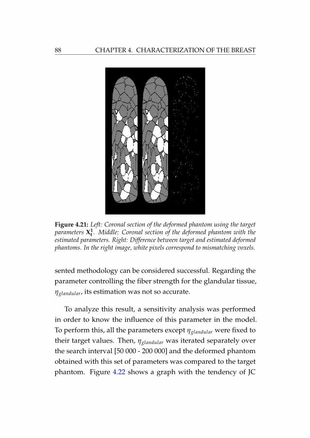
88 CHAPTER 4. CHARACTERIZATION OF THE BREAST
Figure 4.21: Left: Coronal section of the deformed phantom using the targetparameters X1
t . Middle: Coronal section of the deformed phantom with theestimated parameters. Right: Difference between target and estimated deformedphantoms. In the right image, white pixels correspond to mismatching voxels.
sented methodology can be considered successful. Regarding theparameter controlling the fiber strength for the glandular tissue,ηglandular, its estimation was not so accurate.
To analyze this result, a sensitivity analysis was performedin order to know the influence of this parameter in the model.To perform this, all the parameters except ηglandular were fixed totheir target values. Then, ηglandular was iterated separately overthe search interval [50 000 - 200 000] and the deformed phantomobtained with this set of parameters was compared to the targetphantom. Figure 4.22 shows a graph with the tendency of JC

4.5. BIOMECHANICAL MODELING OF THE BREAST TISSUES 89
Figure 4.22: Sensitivity test over the glandular tissue. JC and MHD in termsof ηglandular. The dotted line is the corresponding value to the target phantom.
and MHD when varying ηglandular over the initial search interval.Values of JC>0.93 and MHD<1 voxels in the whole range provedthe low influence of this parameter in the model.
The η parameters take into account two effects: gravity forceand influence of Cooper’s ligaments. On one hand, the breast issubjected to initial strains-stresses due to the gravity force in bothstates, compressed and uncompressed. Ideally, the deformationcaused by the gravity force must be considered separately of thetissue constitutive model. Unfortunately, knowing the non-strainstate of the breast is something that is still being investigated[Rajagopal et al., 2008]. On the other hand, the influence of theCooper’s ligaments was modeled only in one direction as statedin [Han et al., 2011]. Since they have an unknown effect on themodel, the effect of these ligaments should be better modeled inthe three directions of the space. This would involve that new

90 CHAPTER 4. CHARACTERIZATION OF THE BREAST
parameters were added to the model. Nevertheless, they couldalso be estimated with the proposed methodology.
Regarding the anisotropic parameter for the fat tissue, η f at, itsestimation was more accurate with an error lower than 13%. Thisdiscrepancy with the estimation of ηglandular may be due to thehigher presence of fat tissue in the breast as well as the higherinfluence of the Cooper’s ligaments in this tissue. This resultsin a higher effect of η f at on the model compared to the effect ofηglandular.
It is important to highlight the importance of JC and MHD,which indicate how accurate the estimation was. The best esti-mated set of parameters were for Phantoms #2 and #6, where theJC value was about 0.99 and the MHD value was 0.2 voxels (1vox = 200 µm). These are good indicators of the accuracy of theestimated parameters which, especially in these cases, were veryclose to the target parameters with errors lower than 1% for E f at
and Eglandular and lower than 5% for η f at.
As for the estimation of the whole model of the breast, includ-ing the skin, the accuracy of the elastic parameters showed errorslower than 8% (Table 4.6). The addition of the skin to the modeldid not decrease the performance of the methodology. In this case,the estimated elasticity for the skin was achieved with a 4.56% ofrelative mean error which indicates a great influence in the breastmodel as reported in [Solves Llorens et al., 2012]. On the otherhand, the estimation of the η parameters showed an accuracy inconsonance with the first two experiments, where ηglandular didnot induce much variability within the search range.

4.5. BIOMECHANICAL MODELING OF THE BREAST TISSUES 91
The number of elements of the FE mesh also influenced thesearch algorithm. Increasing the element density would impacthighly the time needed to solve the contact problem but wouldalso increase the accuracy of the search. Furthermore, reducing thesearch intervals would cause the algorithm to converge faster byreducing the search space. In this paper, those intervals were setparticularly wide in order to prove the suitability of the methodol-ogy in case of barely knowing the elastic parameters of the differ-ent tissues. Moreover, increasing the complexity of the problem byusing a biomechanical model with more parameters would causethe algorithm to converge slower. Nevertheless, the methodologycould still be applied since genetic heuristics are very efficient tohandle problems with many variables to optimize.
The application of the methodology to real breasts should con-sider additional factors such as segmentation discrepancies, theheterogeneity of the same tissue type along the breast and thepresence of the pectoral muscle. Despite the higher complexityof the internal distribution of the breast tissues, the MRI can besegmented as detailed in [Solves Llorens et al., 2012] and the com-parison between the real compressed MRI and each candidatebiomechanical model can follow the same procedure. In orderto know the accuracy of the estimation of the parameters in realcases, the values of JC and MHD can be analyzed. The closer JC isto 1 and MHD is to 0, the more accurate the estimated parametersof the model are.

92 CHAPTER 4. CHARACTERIZATION OF THE BREAST
4.6 Conclusions
The estimation of the biomechanical parameters of the breasttissues was performed using a software phantom which generatedthe anatomy of the breast allowing the simulation of the breastcompression in an MRI-guided biopsy device. Furthermore, thequality of the finite element mesh used for modeling the breastinternal tissues was analyzed. Homogeneous meshes proved toperform better for the simulation of the mammographic compres-sion. This type of mesh is able to accelerate the finite elementsimulation and provides more stability.
The application of the proposed methodology to the breast mayallow the in-vivo estimation of the patient-specific biomechanicalproperties of the breast internal tissues. The tissues were this waycharacterized by the determination of the elastic constants of ananisotropic hyperelastic model for the fat and glandular tissuesand for an isotropic elastic model in the case of the skin.
The genetic algorithm was able to find a set of elastic constantsalmost identical to the target ones without knowing anythingabout the original behavior and in a wide search space. The per-formance of the methodology was proved with breast phantomsachieving an estimation error of less than 10%.
The methodology to characterize the constitutive model of realbreasts would follow the same procedure. The 3D MRI image of acontrolled compression of the breast on the MRI-guided biopsydevice can be used as a target deformation and the MRI imageof the uncompressed breast can be used to perform the search.
4.6. CONCLUSIONS 93
However, in the case of real breasts, there are some external vari-ables that should be taken into account as boundary conditionssuch as the variability of the biomechanical behavior of the sametissue within the breast, segmentation errors, the gravity effect,the position of the breast in the device or the attachement to thepectoral muscle.


Chapter 5
Characterization of thebiomechanical behavior ofthe cornea
This chapter presents a methodology for the in-vivo estimation ofthe elastic constants specific for the patient of the biomechanicalmodel that characterize the human cornea. The Corvis® ST devicewas used to obtain a video sequence of the cornea deformation.Using the images of the deformed cornea from this sequence, asearch algorithm iterates over the elastic constants to simulatea deformation as close as possible to the real deformed cornea.The methodology was applied to 24 different corneas from 12volunteer patients estimating the hyperelastic behavior of thecorneal tissue specific for each eye of each patient [Lago et al.,2014b].
95

96 CHAPTER 5. CHARACTERIZATION OF THE CORNEA
5.1 Cornea anatomy
The cornea is the most external part of the ocular globe andprotects the eye from external interactions. It has a shape of aregular concave-convex lens and, with approximately 43 diopters,has the highest optical power of the eye although having a fixedfocus. The diameter of the cornea is about 12 mm and its thicknessis between 400 µm and 600 µm, being thiner in the center than inthe periphery. The cornea is attached to the sclera in its periphery.
The human cornea is formed by five layers as it is shown inFigure 5.1. From the most exterior layer to the most interior layer,they are:
Corneal epithelium: the only layer which is in contact withthe air, protecting the rest of layers.
Bowman’s Layer: this layer of about 14 µm is made by colla-gen fibers and protects the corneal stroma.
Corneal Stroma: the main component of the cornea repre-senting up to a 90% of it. It is made by transparent collagenfibers in different parallel layers. The orientation of thefibers is mostly in vertical and horizontal directions in thecenter and following the circumference in the border. Thisorientations confer the cornea an anisotropic behavior.
Descemet’s Membrane: the base of the corneal endotheliumis this acellular membrane of about 10 µm of thickness alsomade by collagen fibers.

5.2. BIOMECHANICAL MODEL OF THE CORNEA 97
Figure 5.1: Schematic of the layers of the cornea.
Corneal Endothelium: the interior surface of the cornea iscovered by this layer of about 5 µm of thickness. This layeris in charge of the impediment of external bodies enteringthe ocular globe and of the nutrition of the rest of the cornea,since it is not vascularized.
5.2 Biomechanical model of the cornea
The human cornea is considered to be an anisotropic, hyperelas-tic and incompressible tissue [Elsheikh et al., 2007]. Many differentmodels have been presented in the literature so far [Kaliske, 2000;Dupps and Wilson, 2006; Lanchares et al., 2008; Nguyen et al.,2008; Pandolfi et al., 2009; Studer et al., 2010]. Even though eachone has its own benefits, all of them rely on the estimation of thebiomechanical parameters that define the model. Most of themhave measured these parameters using ex-vivo human corneasfrom an eye bank [Wollensak et al., 2003; Elsheikh et al., 2007].Others, however, have used the material properties of animalcorneas also estimated ex-vivo [Ahearne et al., 2007; Boyce et al.,

98 CHAPTER 5. CHARACTERIZATION OF THE CORNEA
2007]. The algorithm presented in this thesis is able to estimatein-vivo the elastic constants of any biomechanical model proposedfor the human cornea.
In this work, the human cornea was considered as a homoge-neous tissue and a second order hyperelastic Ogden model waschosen since it provides enough complexity to prove the method-ology without disregarding its realism. In addition, this modelhas been proved to be suitable to simulate the biomechanical be-havior of soft tissues. In particular for the behavior of the liver[Martínez-Martínez et al., 2013b].
The energy potential function of the N-order Ogden model isdefined in Eq. 5.1.
WO =N
∑i=1
µi
αi(λ
αi1 + λ
αi2 + λ
αi3 − 3) +
N
∑i=1
K0i
2(J − 1)2i (5.1)
where N stands for the order; µi and αi stand for the elasticparameters; λ1, λ2 and λ3 are the deviatoric stretches; K0i is theBulk modulus; and J is the determinant of the elastic deformationgradient.
The chosen order for the Ogden model was 2. This ensuredenough complexity in the model without detriment of its realism.Note that the coefficient K0i was fixed to 107 Pa thus assuming thatthe cornea is incompressible [Lanchares et al., 2008]. Therefore,the parameters to be estimated in the model for the cornea werethe following: 〈µ1, α1, µ2, α2〉.

5.3. ESTIMATION OF THE BIOMECHANICAL PROPERTIES 99
5.3 Estimation of the biomechanical properties
The methodology presented here relies on the simulation ofthe deformation of the cornea when applying an air jet for mea-suring the IOP. This process is known as non-contact tonometry.The Corvis® ST device presented in Section 2.3 was used in theophtalmologic clinic Fisabio Oftalmología Médica to take images ofthe cornea during the air pressure loading, thus obtaining a se-quence of images from the initial state, passing through the state ofmaximum deformation, and eventually ending in an undeformedstate. The simulation of the cornea deformation was performedusing the Finite Element Method (FEM), which has been provedto be suitable for large deformations [Glass et al., 2008; Lanchareset al., 2008]. Both segmentation and meshing of the cornea wereperformed using a MATLAB® script, which also controlled thesubsequent iterative search algorithm.
A 2D finite element mesh was constructed from the initial2D slice using 6-node triangles (Figure 5.2). The nodes of themesh corresponding to the edge of the peripheral cornea wererestricted in all directions representing the anchoring with thesclera, which is thought to be 5 times stiffer than the cornea. Theair jet was applied at the apex of the cornea with an average forceof 15 mmHg and an estimated diameter of 3 mm, according to themanufacturer’s indications.
Additionally, the state of maximum deformation of the corneawas taken from the high-speed video after the air jet application.The deformed cornea was segmented in order to compare thebiomechanical simulation of its deformation with the real one.

100 CHAPTER 5. CHARACTERIZATION OF THE CORNEA
Figure 5.2: Meshing of the cornea from the 2D image
Since the initial state of the cornea is actually subjected to theIOP and cannot be considered to be an undeformed state, thefirst step was to reproduce the deformed state due to the IOPby estimating the initial stresses to which the cornea is subjected.This process is independent of the tonometer used to measurethe IOP. It is also independent of the deformation of the corneacaused by the air jet and it was performed before its simulation.After the deformed cornea was segmented, the initial stresses wereextracted by the iterative algorithm within the parameter search.The application of the initial stresses on the biomechanical modelresulted in the initial state of the cornea. Then, the air jet wasapplied at the center of the cornea with the corresponding forceand a new FE simulation was performed. This was carried out foreach set of parameters proposed by the search algorithm.

5.3. ESTIMATION OF THE BIOMECHANICAL PROPERTIES 101
Figure 5.3: The image of the cornea is segmented and meshed in both deformedand undeformed status. The IOP is applied to the undeformed model in order toobtain the initial stresses that are used to simulate the deformation due to the airjet. Finally, the simulated deformation is compared with the real deformation ofthe cornea, and the GSF value is retrieved.

102 CHAPTER 5. CHARACTERIZATION OF THE CORNEA
5.4 Search algorithm
The search algorithm uses the parameter optimization method-ology as described in Section 3.2. In this case, the fit function tooptimize was the dissimilarity of the simulated deformed corneaand the real deformed cornea. The difference was calculated usingthe Geometric Similarity Function (GSF) which was described inSection 3.3, Eq. 3.31.
The methodology for estimating the parameters of the modelhas three steps: Initialization, Generation and Termination. Figure5.3 shows the generation step for each candidate set of parameters.
1. Initialization: the algorithm generates an initial random pop-ulation of elastic parameters X0 within a given interval foreach parameter. Additionally, the real deformed cornea is seg-mented.
2. Generation: successive populations Xi are generated iterativelyby means of the following steps:
i. The initial stress is calculated for each individual set ofparameters as follows:
a. The IOP is applied to the internal surface of the cornea,considering its original state as a non-deformed state.
b. The FEM simulates this loaded state with the Ogdenmodel and the set of elastic constants estimated in eachcase by the search algorithm. This way, the stresses inthe cornea are extracted.

5.4. SEARCH ALGORITHM 103
c. The extracted stresses are applied to the cornea as initialstresses along with the IOP.
d. Steps a., b., and c. are iterated until the displacement ofthe cornea is negligible.
e. The final stresses are obtained and used as the initialstress state for further deformation.
ii. The air jet is applied to the model with the initial stress, andthe FEM is solved using each individual set of parameters.
iii. The GSF between each simulated deformation of the corneaand the real deformation is evaluated in the current popu-lation.
iv. The best individual sets are selected and tagged as parents.Additionally, the best parents are selected as elite.
v. Children are generated both by combining parents (cross-over) or by changing a parent randomly (mutation).
vi. A new population is generated by joining children andelite.
3. Termination: step 2 is iterated until a stop condition is triggered.
The stop condition can be from a maximum number of iter-ations, a sensitivity test between two iterations, or a timer. Theparameters that achieve the best GSF value X, which correspondsto the deformation that is the most similar to the real one, are des-ignated as the estimated parameters of the biomechanical model.

104 CHAPTER 5. CHARACTERIZATION OF THE CORNEA
As well as in the case of the breast, the genetic algorithm im-plemented in MATLAB® was used for the iterative search [Chip-perfield and Fleming, 1995]. The search was parallelized in thecores of the computer to accelerate the process.
5.5 Results
First, a synthetic experiment was performed in order to provethe methodology. The same cornea was deformed with two targetsets of elastic constants of the biomechanical model. The targetsets were X1 : 〈µ1 = 11000, α1 = 30, µ2 = 35000, α2 = 80〉 andX2 : 〈µ1 = 36000, α1 = 50, µ2 = 32500, α2 = 88〉. Their selection wasarbitrary within a previously estimated range. The selection ofIOP and pachymetry was also arbitrary, with the values of thesevariables corresponding to an average value among the obtaineddata of all the patients. The search algorithm was launched inorder to find these given sets of parameters. Table 5.1 shows theresults for the synthetic experiment for the two corneas, includingthe target and estimated parameters, JC and MHD values andthe mean relative error between them. The genetic algorithmstopped when the 5 last generations were not able to improve thefit function more than 10−6.
Afterward, 24 samples from 12 patients with healthy corneabetween the ages of 25 and 40 years old were used to apply themethodology. These patients were volunteers who gave informedconsent. The deformations of the corneas were registered by theCorvis® ST device, and the specific value of the IOP and thepachymetry were measured for each cornea. The size of the pixels

5.5. RESULTS 105
Table 5.1: Target (Tg.), estimated parameters (Est.) and mean relative error(RE) for the synthetic experiment.
IOP Pachy. µ1 α1µ2 α2 JC MHD
(mmHg) (µm) (Pa) (Pa) (µm)
Tg. X1 10.5 595 11 000 30 35 000 80 - -Est. X1 10 711 31.32 33 751 82.44 0.99 4.6RE (%) - - 2.63 4.4 3.6 3.05 - -
Tg. X2 10.5 595 36 000 50 32 500 88 - -Est. X2 34 031 50.07 32 694 89.71 0.99 4.8RE (%) - - 5.47 0.14 0.6 1.94 - -
Mean - - 4.05 2.27 2.1 2.5 - -RE (%)
of the Corvis® ST images was 2 µm.
Regarding the configuration of the genetic algorithm, the pop-ulation was established to 84 enable the pararellization among the12 cores of the computer. The percentage of crossover generatedchildren was set to 80% and set to 20% for mutation and the elitecount was 2, which are the MATLAB® default values. The numberof generations was 15 since this configuration has provided goodresults in previous works [Martínez-Martínez et al., 2013b]. In anycase, these parameters can be changed in order to customize thealgorithm configuration for each patient.
The biomechanical behavior of the 24 corneas were character-ized, estimating the elastic constants of each one for the second-order Ogden model. Table 5.2 shows the estimated parameters forthe left and right corneas for all of the patients as well as the JCand MHD values and the mean relative error committed.

106 CHAPTER 5. CHARACTERIZATION OF THE CORNEA
Table 5.2: Estimated biomechanical constants for Left and Right eyes for eachpatient.
Patient IOP Pachy. µ1 α1µ2 α2 JC MHD
(mmHg) (µm) (Pa) (Pa) (µm)
P115 533 36 508 71.62 13 220 50.17 0.88 22.612 535 25 239 74.73 15 360 79.10 0.88 23
P211.5 499 38 160 91.73 29 536 83.21 0.87 21.211 520 27 220 82.29 31 040 90.24 0.87 23
P312.5 458 27 261 91.06 29 539 46.53 0.84 30.88.5 479 39 492 96.80 14 822 6.13 0.87 24.4
P412.0 520 30 434 92.28 7327 32.74 0.88 2511.5 524 29 588 86.80 31 693 4.37 0.89 19.8
P511.5 580 38 885 77.89 29 141 60.15 0.83 31.411 601 22 120 98.86 13 096 91.94 0.82 32.2
P611 567 24 495 33.37 19 519 80.66 0.88 21.612 568 22 546 74.73 16 950 80.65 0.87 23
P710.5 527 10 978 31.38 33 946 79.82 0.88 21
9 540 22 921 68.02 20 739 70.84 0.88 21
P813 595 39 721 60.32 14 361 69.21 0.90 19.814 588 27 156 18.03 38 305 80.82 0.89 20.6
P913.5 606 17 503 91.11 32 674 53.86 0.89 21.412.5 613 23 161 91.77 3731 78.22 0.89 21
P1014 584 26 511 84.26 23 502 37.52 0.90 20.617 596 5119 97.99 34 767 56.81 0.89 19.8
P118 513 8458 98.14 27 897 91.71 0.80 41
8.5 522 30 704 98.98 15 862 43.92 0.79 43.2
P1212.5 558 12 330 79.19 21 224 83.78 0.83 35.814.5 555 38 327 11.27 32 852 76.47 0.88 24.4
Avg. X 26 034 75.11 22 962 63.70 0.87 25.4Std.Dev. 9960 26.03 9531 25.01 0.03 6.8

5.6. DISCUSSION 107
Figure 5.4: Left: segmentation of the original deformation of a real cornea.Center: simulated deformation of the cornea. Right: signed difference of originaland simulated cornea (the gray values are identical in both images; black andwhite values are signed differences).
Figure 5.4 shows, for a real experiment, the original segmentedcornea, the simulated deformed cornea and their differences forone patient. The gray values identify the correspondence betweenthe two segmentations while the black and white pixels representthe signed differences (positive or negative).
5.6 Discussion
The estimated parameters for the synthetic cases proved thatthe methodology allows to obtain a biomechanical model thatis very similar to the target one. A mean relative error of lessthan 5% in the estimation of the µ parameters and an error ofaround 2.5% in the estimation of α parameters indicate a verysmall deviation from the target parameters. Even though GSF isvery useful for performing the iterative search since it considers

108 CHAPTER 5. CHARACTERIZATION OF THE CORNEA
both overlap and distance, it is hard to translate its values intoa real meaning. Therefore, only JC and MHD values are used tointerpret the results. JC showed a value of 0.99 (99% overlap),and MHD showed a maximum distance of less than 5 µm, whichindicates that the simulated deformation is virtually identical tothe target deformation.
Moving on to the real corneas, the differences between pixelsobserved in Figure 5.4 show a thin line of non-matching pixelsalong the surface of the cornea (internal and external). Table5.2 shows that this distribution of non-matching pixels led toJC values of 87% which means that the majority of the corneatissue is overlapping. Additionally, having as many white pixelsas black pixels indicates that the maladjustment is distributedall along the surface and in the same proportion. On the otherhand, the MHD values showed that the distances between thesimulated and real deformed cornea were, on average, close to25 µm (5% of the average corneal thickness) which indicated thegreat resemblance of the two images. Therefore, the JC and MHDvalues allow knowing how good the adjustment has been, whichgives an idea about the reliability of the estimated model for thatspecific patient.
The parameters of the Ogden model obtained between individ-ual patients proved to be very different due to the high variabilityin composition and heterogeneity of the population. Averagevalues of 26034 ± 9960 Pa and 22962 ± 9531 Pa for µ1 and µ2,respectively, and 75.11± 26.03 and 63.70± 25.01 for α1 and α2,respectively, are in consonance with previous studies that pointedout this variability [Elsheikh et al., 2007].

5.6. DISCUSSION 109
Even though an isotropic hyperelastic Ogden model was usedto prove the algorithm, the methodology presented here can beused with any other biomechanical model chosen to represent thereal behavior of the cornea, even adding more complexity likeconsidering anisotropy or viscoelasticity. The only difference willbe the number of parameters that the genetic algorithm has tohandle and the consequent computation time necessary.
The Corvis® ST device used for the image acquisition provedto be suitable for this methodology even though more complexpersonalized devices could be used to characterize the anisotropyor viscoelasticity of the model. This is the only device currentlyon the market that can provide the information for the in-vivocharacterization of the human cornea. If more information of theundeformed and deformed cornea (such as a 3D reconstruction ora different type of deformation) were available, this methodologycould achieve much more accurate results.
The worst values of JC and MHD appeared in cases wherethe position of the air jet was not exactly aimed at the apex ofthe cornea, while, in the simulated model, it is always applied atit. Therefore, the image acquisition must be carefully performedin order to avoid inaccurate and unreliable results. Correctingthese abnormalities can lead to greater values of JC (closer to thoseobtained in the synthetic experiments), which would guarantee alower error in the parameter estimation.
This methodology was proved to be suitable in a simple 2Dmodel of the cornea. Therefore, having a 3D geometry of thecornea would increase the accuracy of the estimated biomechan-

110 CHAPTER 5. CHARACTERIZATION OF THE CORNEA
ical model and it would broaden the applications of having abiomechanical characterization of the corneal tissue. Moreover,with these simulated deformations, additional physiological prop-erties of the cornea could also be inferred.
The elastic parameters of the average cornea may also be use-ful to construct a generic biomechanical model of the humancornea. Therefore, the average elastic parameters were also usedto simulate the air jet and compared with the real deformationof each patient. The results of the simulation with the averagecornea led to JC values of 0.536±0.256 and average MHD valuesof 79.38±163.77 µm which indicates that the average cornea is notuseful for every patient.
5.7 Conclusions
In this chapter, the methodology for the in-vivo estimation ofthe elastic constants was applied to model the human cornealtissue. Two experiments were carried out, a synthetic experimentwith the aim to prove the performance and evaluate the accuracyof the methodology, and a second experiment with real corneas.The iterative search was able to characterize the biomechanicalbehavior of the cornea of each patient with a hyperelastic, second-order Ogden model. Twenty-four patient-specific biomechanicalmodels were constructed which proved to be very similar to thereal behavior of the patients’ corneas.
This methodology is easily applicable to any biomechanicalmodel adding also anisotropy and viscoelasticity. Furthermore,being able to estimate the biomechanical behavior of the cornea

5.7. CONCLUSIONS 111
would also allow physiological and optical parameters like hys-teresis or refractive power to be inferred, and would also allow thecornea response to be simulated during and after refractive sur-gical procedures. Additionally, a very interesting line of researchwould be to classify the cornea behavior taking into account dif-ferent factors such as gender, age or, ocular diseases.


Chapter 6
Conclusions
This dissertation has presented a methodology for the in-vivo char-acterization the biomechanical behavior of two different organs:the breast and the cornea. The methodology can be translated toconstruct a biomechanical model for the breast and for the corneawithout the need of any invasive intervention, and within theclinical protocols.
The methodology considers the estimation of the elastic con-stants as a parameter optimization problem. A genetic heuristicwas selected to drive the search algorithm due to its ability to findthe minimum of a complex function that may present many localminima. The optimization was carried out using, as fit function,a volumetric similarity function, the GSF, which considers bothoverlap and distance between the real deformation of an organand its simulation.
113

114 CHAPTER 6. CONCLUSIONS
6.1 Summary of contributions
Selection of the best coefficients for volume comparison:This experiment tested the behavior of several coefficientsused traditionally for validation of segmentations in orderto compare the similarity between two volumes. It wasproved that the combination of Jaccard Coefficient and theModified Hausdorff Distance allows the evaluation of therealism of a simulation of the deformation of an organ by itsbiomechanical model.
Mesh quality study: This study proved the high importanceof the quality of the mesh elements in order to get reliablesimulations and avoid convergence problems. The use ofa homogeneous mesh instead of an adaptive mesh is moresuitable to simulate complex internal tissue distributions ascan be found in the breast.
Biomechanical parameter estimation for the breast tissues:In the case of the breast, the mammographic compressionduring an MRI biopsy is able to retrieve the 3D volume ofthe compressed breast. A biomechanical model simulatingthe same compression was used to create software phantomstrying to mimic the current procedure. The application ofthe parameter estimation to the breast phantoms achievedan accuracy of about 90%.
Biomechanical parameter estimation for the cornea: Fi-nally, the parameter estimation was also used to create abiomechanical model of the human cornea taking advantage

6.2. FUTURE WORK 115
of the tonometry. This technique is used to measure the IOPof the eye by applying an air jet to the cornea. The Corvis®
ST device records the deformation over time of the cornea.These images were used to create a biomechanical modelsimulating the air jet. 24 corneas were characterized and avalidation with synthetic experiments proved to obtain anaccuracy of above 95%.
6.2 Future work
Since the methodology proposed in this thesis was tested, inthe case of the breast, with software phantoms, the next step inthis research will be to apply it to real patients. First, the breastwill be segmented to separate the different internal tissues. The ho-mogeneous meshing algorithm will be used to mesh the complexinternal structures such as the glandular tissue thus improvingthe convergence of the simulation. The force applied by the MRIscanner can be obtained using a force sensor on the compressionplates and the simulation of the compression can be performedas it was described for the phantoms. Finally, the iterative searchwill be able to estimate the elastic constants that define the biome-chanical behavior of the breast tissues for each specific patient.This model could be used to locate tumors in different positionsof the breasts such as the prone to supine deformation or for theregistration between an X-ray mammogram and the MRI.
In the case of the cornea, after estimating the biomechanicalbehavior of the tissue, some pathologies can be detected since theymodify the stiffness of the tissue. Using the 3D reconstruction of

116 CHAPTER 6. CONCLUSIONS
the cornea that can be obtained from devices such as Pentacamtogether with the biomechanical model previously estimated forthe patients the deformation resultant of the insertion of intra-corneal rings for patients with keratoconus could be predicted.This way, the position, angle, and ring size will be optimized foreach patient. Additionally, some physiological parameters such asthe hysteresis or the corneal resistance factor can be estimated.
6.3 Final considerations
The characterization of the behavior of soft tissue is the coreof its biomechanical simulation and the responsible of achievingrealistic results. With the guarantee of estimating how an organ re-acts to external interactions, surgeons can count on having virtualenvironments capable to simulate real interventions. This way,surgeons can prevent critical scenarios, train their skills, and planfuture interventions, as well as use them for surgical guidance.
The development of a complete virtual body that considers allthe possible interactions is still far in the future. However, thefirst steps in this direction are to provide a realistic behavior of thetissues present in the organs. Unfortunately, computational costsare still a big barrier since the time needed for solving the FEMis too high. Even though some meshfree methods are currentlygaining popularity in numerical simulation they are still very timeconsuming [Liu, 2010].
The ultimate goal is the creation of a realistic simulation of thewhole human body in real time, but this is something that, to date,is still only in our imagination.

Generated literature
Journal papers
Lago, M. A., Rupérez, M. J., Martínez-Martínez, F., Monserrat,C., Larra, E., Güell, J. L. and Peris-Martínez, C. (2014). A newmethodology to in-vivo estimate the elastic constants thatcharacterize the patient-specific biomechanical behavior ofthe human cornea. Journal of Biomechanics (major revisions)
Lago, M. A., Rupérez, M., Martínez-Martínez, F., Bakic, P. R.,Maidment, A. D., and Monserrat, C. (2014). Methodologybased on genetic heuristics for in-vivo characterizing thepatient-specific biomechanical behavior of the breast tissues.Expert Systems with Applications (under revision)
117
118 CHAPTER 6. CONCLUSIONS
International conferences
Lago, M.A., Martínez-Martínez, F., Rupérez, M.J., Monserrat,C., Alcañiz, M. (2012). A study about coefficients to estimatethe error in biomechanical models used to virtually simulatethe organ behaviors. In Proceedings of international conferenceon Medicine Meets Virtual Reality (MMVR), volume 173, pages250–256. IOS Press
Lago, M. A., Martínez-Martínez, F., Rupérez, M., Monserrat, C.,and Alcañiz, M. (2012). Breast prone-to-supine deformationand registration using a time-of-flight camera. In Proceedingsof International Conference on Biomedical Robotics and Biomecha-tronics (BioRob), 2012 4th IEEE RAS EMBS, pages 1161–1163.
Lago, M. A., Maidment, A. D., and Bakic, P. R. (2013). Mod-eling of mammographic compression of anthropomorphicsoftware breast phantom using FEBio. In Proceedings of Inter-national Symposium of Computer Methods in Biomechanics andBiomedical Engineering (CMBBE), pages 495–496. This paperobtained the 3rd best student poster award.
Maidment, A. D., Bakic, P. R., Chui, J. H., Avanaki, A. N.,Marchessoux, C., Pokrajac, D. D., Espig, K. S., Kimpe, T.,Xthona, A., Lago, M. A., and Shankla, V. (2013). The roleof virtual clinical trials in preclinical testing of breast imag-ing systems. In Proceedings of the 99th Scientific Assembly andAnnual Meeting (RSNA)

6.3. FINAL CONSIDERATIONS 119
Bakic, P. R., Maidment, A. D., Chui, J. H., Avanaki, A. N.,Marchessoux, C., Pokrajac, D. D., Espig, K. S., Kimpe, T.,Xthona, A., Lago, M. A., and Shankla, V. (2013). Automatedand optimized imaging simulation platform for virtual clini-cal trials of breast cancer screening. In Proceedings of the 99thScientific Assembly and Annual Meeting (RSNA)
Lago, M. A., Rupérez, M., Martínez-Martínez, F., Monserrat, C.(2014). Genetic algorithms for estimating the biomechanicalbehavior of breast tissues . In Proceedings of IEEE-EMBS Inter-national Conferences on Biomedical and Health Informatics (BHI),pages 760–763. This paper obtained the 3rd best student oralcommunication award.
National conferences
Lago, M. A., Monserrat, C., Rupérez, M. J., Solves-Llorens, J. A.,Martínez-Martínez, F., and Alcañiz, M. (2012). Simulaciónde la deformación de la mama en posición supino partiendode imágenes de resonancia magnética y usando una cámaraTime-of-Flight. In Proceedings of II Reunión del Capítulo Españolde la Sociedad Europea de Biomecánica (ESB).
Lago, M. A., Rupérez, M. J., Monserrat, C. (2013). Impact ofthe Meshing Method in the Biomechanical Simulation of theMammographic Compression. In Proceedings of III Reunióndel Capítulo Español de la Sociedad Europea de Biomecánica (ESB),page 38

Bibliography
Ahearne, M., Yang, Y., Then, K., and Liu, K.-K. (2007). An indenta-tion technique to characterize the mechanical and viscoelasticproperties of human and porcine corneas. Annals of BiomedicalEngineering, 35(9):1608–1616. 2 citations in pages 16 and 97.
Alastrué, V., Calvo, B., Pena, E., and Doblaré, M. (2006). Biome-chanical modeling of refractive corneal surgery. Journal of Biome-chanical Engineering, 128(1):150–160. One citation in page 15.
Aspert, N., Santa-Cruz, D., and Ebrahimi, T. (2002). MESH: mea-suring errors between surfaces using the Hausdorff distance.In Proceedings of IEEE International Conference on Multimedia andExpo, ICME ’02., volume 1, pages 705–708 vol.1. One citation inpage 33.
Azar, F. S., Metaxas, D. N., and Schnall, M. D. (2001). A DeformableFinite Element Model of the Breast for Predicting MechanicalDeformations under External Perturbations. Academic Radiology,8(10):965 – 975. One citation in page 76.
121

122 BIBLIOGRAPHY
Bakic, P. R., Albert, M., Brzakovic, D., and Maidment, A. D. A.(2002). Mammogram synthesis using a 3D simulation. I. Breasttissue model and image acquisition simulation. Medical Physics,29(9):2131–2139. 3 citations in pages 53, 56, and 60.
Bakic, P. R., Ng, S., Ringer, P., Carton, A.-K., Conant, E. F., andMaidment, A. D. A. (2010). Validation and optimization of digi-tal breast tomosynthesis reconstruction using an anthropomor-phic software breast phantom. Proceedings of SPIE, 7622:76220F–76220F–9. One citation in page 56.
Bakic, P. R., Zhang, C., and Maidment, A. D. A. (2011). Develop-ment and characterization of an anthropomorphic breast soft-ware phantom based upon region-growing algorithm. MedicalPhysics, 38(6):3165–3176. 5 citations in pages 53, 54, 57, 60,and 146.
Balocco, S., Camara, O., Vivas, E., Sola, T., Guimaraens, L.,Gratama van Andel, H. A. F., Majoie, C. B., Pozo, J. M., Bij-nens, B. H., and Frangi, A. F. (2010). Feasibility of estimatingregional mechanical properties of cerebral aneurysms in-vivo.Medical Physics, 37(4):1689–706. One citation in page 31.
Barr, R. G. (2012). Sonographic breast elastography: A primer.Journal of Ultrasound in Medicine, 31(5):773–783. One citation inpage 13.
Bhatti, S. N. and Sridhar-Keralapura, M. (2012). A novel breastsoftware phantom for biomechanical modeling of elastography.Medical Physics, 39(4):1748–1768. 3 citations in pages 55, 56,and 146.
Bianchi, G., Solenthaler, B., Székely, G., and Harders, M. (2004).

BIBLIOGRAPHY 123
Simultaneous topology and stiffness identification for mass-spring models based on FEM reference deformations. In Proceed-ings of Medical Image Computing and Computer-Assisted Interven-tion (MICCAI 2004), pages 293–301. Springer, Heidelberg. Onecitation in page 27.
Billiar, K. and Sacks, M. (2000). Biaxial mechanical properties ofthe native and glutaraldehyde-treated aortic valve cusp: PartII - A structural constitutive model. Journal of BiomechanicalEngineering-Transactions of the ASME, 122(4):327–335. One cita-tion in page 10.
Bliznakova, K., Bliznakov, Z., Bravou, V., Kolitsi, Z., and Pal-likarakis, N. (2003). A three-dimensional breast software phan-tom for mammography simulation. Physics in Medicine andBiology, 48(22):3699. 3 citations in pages 54, 55, and 146.
Bliznakova, K., Suryanarayanan, S., Karellas, A., and Pallikarakis,N. (2010). Evaluation of an improved algorithm for producingrealistic 3D breast software phantoms: Application for mam-mography. Medical Physics, 37(11):5604–5617. One citation inpage 54.
Boyce, B., Jones, R., Nguyen, T., and Grazier, J. (2007). Stress-controlled viscoelastic tensile response of bovine cornea. Journalof Biomechanics, 40(11):2367–2376. 2 citations in pages 16 and 97.
Bucki, M., Lobos, C., Payan, Y., and Hitschfeld, N. (2011). Jacobian-based repair method for finite element meshes after registration.Engineering with Computers, 27(3):285–297. 2 citations in pages59 and 60.
Burkhart, T. A., Andrews, D. M., and Dunning, C. E. (2013). Finite

124 BIBLIOGRAPHY
element modeling mesh quality, energy balance and validationmethods: A review with recommendations associated with themodeling of bone tissue. Journal of Biomechanics, 46(9):1477 –1488. 2 citations in pages 20 and 59.
Cárdenes, R., de Luis-García, R., and Bach-Cuadra, M. (2009). Amultidimensional segmentation evaluation for medical imagedata. Computer Methods and Programs in Biomedicine, 96(2):108 –124. One citation in page 32.
Carter, F. J., Frank, T. G., Davies, P. J., McLean, D., and Cuschieri,A. (2001). Measurements and modelling of the compliance ofhuman and porcine organs. Medical Image Analysis, 5(4):231 –236. One citation in page 11.
Carter, T., Tanner, C., Beechey-Newman, N., Barratt, D., andHawkes, D. (2008). MR Navigated Breast Surgery: Methodand Initial Clinical Experience. In Medical Image Computing andComputer-Assisted Intervention (MICCAI 2008), volume 5242 ofLecture Notes in Computer Science, pages 356–363. Springer BerlinHeidelberg. 2 citations in pages 12 and 76.
Chatterjee, S., Laudato, M., and Lynch, L. A. (1996). Geneticalgorithms and their statistical applications: an introduction.Computational Statistics & Data Analysis, 22(6):633 – 651. Onecitation in page 27.
Chen, B., Shorey, J., Jr., R. S. S., Richard, S., Thompson, J., Nolte,L. W., and Samei, E. (2011). An anthropomorphic breast modelfor breast imaging simulation and optimization. Academic Radi-ology, 18(5):536 – 546. One citation in page 54.
Chew, P. H., Yin, F. C., and Zeger, S. L. (1986). Biaxial stress-

BIBLIOGRAPHY 125
strain properties of canine pericardium. Journal of Molecular andCellular Cardiology, 18(6):567 – 578. One citation in page 10.
Chipperfield, A. and Fleming, P. (1995). The MATLAB geneticalgorithm toolbox. In Applied Control Techniques Using MATLAB,IEE Colloquium on, pages 10/1–10/4. 2 citations in pages 85and 104.
Chui, J. H., Pokrajac, D. D., Maidment, A. D. A., and Bakic, P. R.(2012). Towards Breast Anatomy Simulation Using GPUs. InDigital Mammography / IWDM, pages 506–513. 3 citations inpages 54, 57, and 80.
Chung, J.-H., Rajagopal, V., Nielsen, P. M., and Nash, M. P. (2008).Modelling mammographic compression of the breast. In MedicalImage Computing and Computer-Assisted Intervention (MICCAI2008), pages 758–765. Springer. One citation in page 74.
Clark, R. (1973). Stress-strain characteristics of fresh and frozenhuman aortic and mitral leaflets and chordae tendineae - im-plications for clinical use. Journal of Thoracic and CardiovascularSurgery, 66(2):202–208. One citation in page 10.
Cox, M. A., Driessen, N. J., Boerboom, R. A., Bouten, C. V., andBaaijens, F. P. (2008). Mechanical characterization of anisotropicplanar biological soft tissues using finite indentation: Experi-mental feasibility. Journal of Biomechanics, 41(2):422 – 429. Onecitation in page 11.
Cox, S., Mithraratne, K., and Smith, N. (2007). An anatomicallybased finite element model of the lower limbs in the seated pos-ture. In Engineering in Medicine and Biology Society, 2007. EMBS

126 BIBLIOGRAPHY
2007. 29th Annual International Conference of the IEEE, pages 6326–6329. One citation in page 20.
Crum, W. R., Tanner, C., and Hawkes, D. J. (2005). Anisotropicmulti-scale fluid registration: evaluation in magnetic resonancebreast imaging. Physics in Medicine and Biology, 50(21):5153. Onecitation in page 30.
Curry, T., Dowdey, J., and Murry, R. (1990). Christensen’s Physics ofDiagnostic Radiology. Lea & Febiger. One citation in page 50.
Dance, D. R., Hunt, R. A., Bakic, P. R., Maidment, A. D. A., Sand-borg, M., Ullman, G., and Alm Carlsson, G. (2005). Breastdosimetry using high-resolution voxel phantoms. RadiationProtection Dosimetry, 114(1-3):359–363. One citation in page 54.
Deenadayalu, C., Mobasher, B., Rajan, S., and Hall, G. (2006).Refractive change induced by the LASIK flap in a biomechanicalfinite element model. Journal of Refractive Surgery, 22(3):286–292.One citation in page 15.
del Palomar, A. P., Calvo, B., Herrero, J., López, J., and Doblaré,M. (2008). A finite element model to accurately predict realdeformations of the breast. Medical Engineering and Physics,30(9):1089 – 1097. 3 citations in pages 12, 73, and 76.
delBuey, M., Lanchares, E., Cristobal, J., Calvo, B., and Lavilla,L. (2010). Comparative biomechanical analysis of combinedtreatments for keratoconus. In proceedings of ASCRS Symposiumand Congress. One citation in page 15.
Dice, L. R. (1945). Measures of the amount of ecologic association

BIBLIOGRAPHY 127
between species. Ecology, 26(3):297–302. One citation in page32.
Diekmann, F., Meyer, H., Diekmann, S., Puong, S., Muller, S., Bick,U., and Rogalla, P. (2009). Thick slices from tomosynthesis datasets: Phantom study for the evaluation of different algorithms.Journal of Digital Imaging, 22(5):519–526. One citation in page 54.
Dubuisson, M. P. and Jain, A. K. (1994). A modified Hausdorffdistance for object matching. In Proceedings of 12th InternationalConference on Pattern Recognition, pages 566–568. IEEE Comput.Soc. Press. 2 citations in pages 35 and 39.
Dupps, W. J. and Wilson, S. E. (2006). Biomechanics and woundhealing in the cornea. Experimental Eye Research, 83(4):709 – 720.One citation in page 97.
Edelsbrunner, H. (2001). Geometry and Topology for Mesh Generation.Cambridge. One citation in page 62.
Egan, R. (1988). Breast Imaging: Diagnosis and Morphology of BreastDiseases. W. B. Saunders. One citation in page 46.
Elsheikh, A., Wang, D., Brown, M., Rama, P., Campanelli, M., andPye, D. (2007). Assessment of corneal biomechanical propertiesand their variation with age. Current Eye Research, 32(1):11–19.4 citations in pages 15, 16, 97, and 108.
Field, D. (2000). Qualitative Measures for Initial Meshes. In Inter-national Journal of Numerical Methods in Engineering, volume 47,pages 887–906. One citation in page 62.
Fogel, D. (1995). Evolution Computation: Toward a New Philosophy of

128 BIBLIOGRAPHY
Machine Intelligence. Press, Piscataway, NJ. One citation in page26.
Fung, Y. (1972). Stress-Strain-History Relations of Soft Tissues inSimple Elongation. In Biomechanics: Its Foundations and Objec-tives. Prentice-Hall, Englewood Cliffs, NJ. One citation in page9.
Fung, Y. (1974). Biorheology of loose connective tissues, especiallyblood vessels. In Biopolymere und Biomechanik von Bindegewebssys-temen, pages 191–210. Springer Berlin Heidelberg. One citationin page 10.
Fung, Y. C. (1993). Biomechanics: Mechanical Properties of LivingTissues. Hardcover, Springer US. One citation in page 20.
Gee, M. W., Förster, C., and Wall, W. A. (2010). A computationalstrategy for prestressing patient-specific biomechanical prob-lems under finite deformation. International Journal for NumericalMethods in Biomedical Engineering, 26(1):52–72. One citation inpage 11.
Gefen, A. and Dilmoney, B. (2007). Mechanics of the normalwoman’s breast. Technology and Health Care, 15(4):259–271. 6citations in pages 13, 20, 47, 64, 73, and 76.
Gefen, A., Shalom, R., Elad, D., and Mandel, Y. (2009). Biomechan-ical analysis of the keratoconic cornea. Journal of the MechanicalBehavior of Biomedical Materials, 2(3):224 – 236. One citation inpage 15.
Ghista, D. and Rao, A. (1973). Mitral-valve mechanics - stress-strain characteristics of excised leaflets, analysis of its functional

BIBLIOGRAPHY 129
mechanics and its medical application. Medical & BiologicalEngineering, 11(6):691–702. One citation in page 10.
Glass, D. H., Roberts, C. J., Litsky, A. S., and Weber, P. A. (2008).A viscoelastic biomechanical model of the cornea describingthe effect of viscosity and elasticity on hysteresis. InvestigativeOphthalmology and Visual Science, 49(9):3919–3926. 2 citations inpages 16 and 99.
Goldmann, H. and Schmidt, T. (1957). Über Applanationstonome-trie. Ophthalmologica, 134(4):221–242. One citation in page 17.
Gow, B. S. and Vaishnav, R. N. (1975). A microindentation tech-nique to measure rheological properties of the vascular intima.Journal of Applied Physiology, 38(2):344–350. One citation in page11.
Greenleaf, J. F., Fatemi, M., and Insana, M. (2003). Selected meth-ods for imaging elastic properties of biological tissues. AnnualReview of Biomedical Engineering, 5(1):57–78. One citation in page13.
Han, L., Hipwell, J., Mertzanidou, T., Carter, T., Modat, M.,Ourselin, S., and Hawkes, D. (2011). A hybrid FEM-basedmethod for aligning prone and supine images for image guidedbreast surgery. In IEEE International Symposium on BiomedicalImaging: From Nano to Macro, pages 1239–1242. 3 citations inpages 12, 58, and 89.
Han, L., Hipwell, J. H., Tanner, C., Taylor, Z., Mertzanidou, T.,Cardoso, J., Ourselin, S., and Hawkes, D. J. (2012). Developmentof patient-specific biomechanical models for predicting large

130 BIBLIOGRAPHY
breast deformation. Physics in Medicine and Biology, 57(2):455. 7citations in pages 14, 20, 46, 61, 77, 78, and 84.
Han, L., Noble, J., and Burcher, M. (2003). A novel ultrasoundindentation system for measuring biomechanical properties ofin-vivo soft tissue. Ultrasound in Medicine & Biology, 29(6):813 –823. One citation in page 11.
Harb, N., Labed, N., Domaszewski, M., and Peyraut, F. (2011). Anew parameter identification method of soft biological tissuecombining genetic algorithm with analytical optimization. Com-puter Methods in Applied Mechanics and Engineering, 200(4):208 –215. 2 citations in pages 13 and 20.
Hausdorff, F. (1962). Set theory, 2nd Ed. Chelsea Pub. Co. Onecitation in page 33.
Hesselink, J. R. (2006). Basic Principles of MR Imaging. Online.One citation in page 50.
Hibbitt, K. and Sorensen (2001). ABAQUS/CAE User’s Manual.Hibbitt, Karlsson & Sorensen, Incorporated. One citation inpage 68.
Hjortdal, J. Ø. (1995). Extensibility of the normo-hydrated humancornea. Acta Ophthalmologica Scandinavica, 73(1):12–17. Onecitation in page 15.
Hori, R. and Mockros, L. (1976). Indentation tests of human articu-lar cartilage. Journal of Biomechanics, 9(4):259 – 268. One citationin page 11.
Hsu, C. M. L., Palmeri, M. L., Segars, W. P., Veress, A. I., and III,J. T. D. (2011). An analysis of the mechanical parameters used

BIBLIOGRAPHY 131
for finite element compression of a high-resolution 3D breastphantom. Medical Physics, 38(10):5756–5770. 2 citations in pages12 and 20.
Humphrey, J., Halperin, H., and Yin, F. (1991). Small indentationsuperimposed on a finite equibiaxial stretch implications forcardiac mechanics. Journal of Applied Mechanics-Transactions ofthe ASME, 58(4):1108–1111. One citation in page 11.
Huttenlocher, D., Klanderman, G., and Rucklidge, W. (1993). Com-paring images using the Hausdorff distance. IEEE Transactionson Pattern Analysis and Machine Intelligence, 15(9):850–863. Onecitation in page 33.
Jeffrey, B. E. (2004). Static Indentation of Anisotropic Biomate-rials Using Axially Asymmetric Indenters—a ComputationalStudy. Journal of Biomechanical Engineering, 126(4):498–505+. Onecitation in page 11.
Joe, B. (1991). GEOMPACK - a software package for the generationof meshes using geometric algorithms. Advances in EngineeringSoftware, 13:325–331. One citation in page 62.
Johns, P. C. and Yaffe, M. J. (1987). X-ray characterisation of normaland neoplastic breast tissues. Physics in Medicine and Biology,32(6):675. One citation in page 49.
Jong, K. A. (2006). Evolutionary computation: a unified approach. MITPress. One citation in page 26.
Kaliske, M. (2000). A formulation of elasticity and viscoelasticityfor fibre reinforced material at small and finite strains. Computer

132 BIBLIOGRAPHY
Methods in Applied Mechanics and Engineering, 185(4):225 – 243.One citation in page 97.
Kellner, A. L., Nelson, T. R., Cerviño, L. I., and Boone, J. M. (2007).Simulation of mechanical compression of breast tissue. Transac-tions on Biomedical Engineering, 54(10):1885–91. One citation inpage 59.
Kim, J. and Srinivasan, M. (2005). Characterization of viscoelas-tic soft tissue properties from in-vivo animal experiments andinverse FE parameter estimation. Medical Image Computing andComputer-Assisted Intervention (MICCAI 2005), pages 599–606.One citation in page 20.
Kotecha, A., Elsheikh, A., Roberts, C. R., Zhu, H., and Garway-Heath, D. F. (2006). Corneal thickness- and age-related biome-chanical properties of the cornea measured with the ocular re-sponse analyzer. Investigative Ophthalmology and Visual Science,47(12):5337–5347. One citation in page 16.
Krouskop, T. A., Wheeler, T. M., Kallel, F., Garra, B. S., and Hall,T. (1998). Elastic moduli of breast and prostate tissues undercompression. Ultrasonic Imaging, 20(4):260–274. One citation inpage 13.
Lago, M., Martínez-Martínez, F., Rupérez, M., Monserrat, C., andAlcañiz, M. (2012a). A study about coefficients to estimate theerror in biomechanical models used to virtually simulate theorgan behaviors. In Proceedings of International Conference onMedicine Meets Virtual Reality, volume 173, pages 250–256. IOSPress. One citation in page 34.
Lago, M. A., Maidment, A. D., and Bakic, P. R. (2013a). Modeling

BIBLIOGRAPHY 133
of mammographic compression of anthropomorphic softwarebreast phantoms using FEBio. In Proceedings of InternationalSymposium of Computer Methods in Biomechanics and BiomedicalEngineering, pages 495–496. One citation in page 58.
Lago, M. A., Martinez-Martinez, F., Ruperez, M., Monserrat, C.,and Alcaniz, M. (2012b). Breast prone-to-supine deformationand registration using a Time-of-Flight camera. In Proceedings ofInternational Conference on Biomedical Robotics and Biomechatron-ics (BioRob), 2012 4th IEEE RAS EMBS, pages 1161–1163. Onecitation in page 58.
Lago, M. A., Monserrat, C., Rupérez, M. J., Solves-Llorens, J. A.,Martínez-Martínez, F., and M., A. (2012c). Simulación de ladeformación de la mama en posición supino partiendo de imá-genes de resonancia magnética y usando una cámara time-of-flight. In Proceedings of II Reunión del Capítulo Español de laSociedad Europea de Biomecánica (ESB). One citation in page 58.
Lago, M. A., Rupérez, M. J., Martínez-Martínez, F., and Monserrat,C. (2014a). Genetic algorithms for estimating the biomechanicalbehavior of breast tissues. In Proceedings of IEEE-EMBS Inter-national Conferences on Biomedical and Health Informatics (BHI),pages 760–763. One citation in page 46.
Lago, M. A., Rupérez, M. J., Martínez-Martínez, F., Monserrat,C., Larra, E., Güell, J. L., and Peris-Martínez, C. (2014b). Anew methodology to in-vivo estimate the elastic constants thatcharacterize the patient-specific biomechanical behavior of thehuman cornea (major revisions). Journal of Biomechanics. Onecitation in page 95.

134 BIBLIOGRAPHY
Lago, M. A., Rupérez, M. J., and Monserrat, C. (2013b). Impactof the Meshing Method in the Biomechanical Simulation of theMammographic Compression. In Proceedings of Spanish Chapterof the European Society of Biomechanics (ESB), page 38. 2 citationsin pages 59 and 75.
Lamarque, J. (1984). An atlas and text of the breast: clinical radiodi-agnosis. Wolfe medical atlases. Wolfe Medical. One citation inpage 47.
Lanchares, E., Calvo, B., Cristóbal, J. A., and Doblaré, M. (2008).Finite element simulation of arcuates for astigmatism correction.Journal of Biomechanics, 41(4):797 – 805. 5 citations in pages 15,20, 97, 98, and 99.
Lanir, Y. (1979). A structural theory for the homogeneous biaxialstress-strain relationships in flat collagenous tissues. Journal ofBiomechanics, 12(6):423 – 436. One citation in page 20.
Lanir, Y. and Fung, Y. (1974). Two-dimensional mechanical proper-ties of rabbit skin II. Experimental results. Journal of Biomechanics,7(2):171 – 182. One citation in page 10.
Lee, A. W. C., Schnabel, J. A., Rajagopal, V., Nielsen, P. M. F., andNash, M. P. (2010). Breast image registration by combiningfinite elements and free-form deformations. In Proceedings of the10th international conference on Digital Mammography, IWDM’10,pages 736–743, Berlin, Heidelberg. Springer-Verlag. One citationin page 30.
Li, C. M., Segars, W. P., Tourassi, G. D., Boone, J. M., and Dobbins,J. T. (2009). Methodology for generating a 3D computerized
BIBLIOGRAPHY 135
breast phantom from empirical data. Medical Physics, 36(7):3122–3131. 3 citations in pages 54, 55, and 146.
Liu, G. (2010). Meshfree Methods: Moving Beyond the Finite ElementMethod, Second Edition. Taylor & Francis. One citation in page116.
Lockett, H. and Guenov, M. (2008). Similarity measures for mid-surface quality evaluation. Computer-Aided Design, 40(3):368 –380. One citation in page 33.
Luce, D. A. (2005). Determining in-vivo biomechanical proper-ties of the cornea with an ocular response analyzer. Journal ofCataract and Refractive Surgery, 31(1):156 – 162. One citation inpage 16.
Ma, A. K. W., Gunn, S., and Darambara, D. G. (2009). IntroducingDeBRa: a detailed breast model for radiological studies. Physicsin Medicine and Biology, 54(14):4533. One citation in page 54.
Maas, S., Ellis, B., Ateshian, G., and Weiss, J. (2012). FEBio: finiteelements for biomechanics. Journal of Biomechanical Engineering,134(1):011005. One citation in page 69.
Mariappan, Y. K., Glaser, K. J., and Ehman, R. L. (2010). Magneticresonance elastography: A review. Clinical Anatomy, 23(5):497–511. One citation in page 13.
Martínez-Martínez, F., Lago, M. A., Rupérez, M. J., and Monserrat,C. (2013a). Analysis of several biomechanical models for thesimulation of lamb liver behaviour using similarity coefficientsfrom medical image. Computer Methods in Biomechanics andBiomedical Engineering, 16(7):747–757. One citation in page 11.

136 BIBLIOGRAPHY
Martínez-Martínez, F., Lago, M. A., Rupérez, M. J., Monserrat,C., Pareja, E., Cortés, M., López, R., and Brugger, S. (2012). Acomputational method to estimate the elastic parameters ofbiomechanical models for the in-vivo human liver. In Proceed-ings of the 10th International Symposium on Computer Methods inBiomechanics and Biomedical Engineering., CMBBE 2012. 2 cita-tions in pages 20 and 42.
Martínez-Martínez, F., Rupérez, M. J., Martín-Guerrero, J. D., Mon-serrat, C., Lago, M. A., Pareja, E., and López-Andújar, R. (2013b).Estimation of the elastic parameters of human liver biomechani-cal models by means of medical images and Evolutionary Com-putation. Computer Methods and Programs in Biomedicine. 5citations in pages 13, 42, 85, 98, and 105.
Matthews, F. and West, J. (1972). Finite element displacementanalysis of a lung. Journal of Biomechanics, 5(6):591 – 600. Onecitation in page 58.
May-Newman, K. and Yin, F. (1995). Biaxial mechanical-behaviorof excised porcine mitral-valve leaflets. American Journal ofPhysiology-Heart and Circulatory Physiology, 269(4):H1319–H1327.One citation in page 10.
Mehrabian, H., Campbell, G., and Samani, A. (2010). A con-strained reconstruction technique of hyperelasticity parametersfor breast cancer assessment. Physics in Medicine and Biology,55(24):7489. One citation in page 13.
Miller, K. and Lu, J. (2013). On the prospect of patient-specificbiomechanics without patient-specific properties of tissues. Jour-

BIBLIOGRAPHY 137
nal of the Mechanical Behavior of Biomedical Materials, 27(0):154 –166. One citation in page 11.
Mooney, M. (1940). A theory of large elastic deformation. Journalof Applied Physics, 11(9):582–592. One citation in page 25.
Nair, A. U., Taggart, D. G., and Vetter, F. J. (2007). Optimizingcardiac material parameters with a genetic algorithm. Journal ofBiomechanics, 40(7):1646 – 1650. One citation in page 13.
Nava, A., Mazza, E., Furrer, M., Villiger, P., and Reinhart, W. (2008).In-vivo mechanical characterization of human liver. MedicalImage Analysis, 12(2):203 – 216. One citation in page 11.
Netter, F. (1989). Atlas of Human Anatomy. Netter Basic Science.Elsevier Health Sciences. 3 citations in pages 47, 48, and 146.
Nguyen, T. D., Jones, R. E., and Boyce, B. L. (2008). A nonlinearanisotropic viscoelastic model for the tensile behavior of thecorneal stroma. Journal of Biomechanical Engineering, 130(4). Onecitation in page 97.
Nielsen, P. M. F., Malcolm, D. T. K., Hunter, P. J., and Charette,P. G. (2002). Instrumentation and procedures for estimating theconstitutive parameters of inhomogeneous elastic membranes.Biomechanics and Modeling in Mechanobiology, 1(3):211–218. Onecitation in page 10.
Nishikawa, R., Glick, S., Bakic, P., and Reiser, I. (2011). 3D BreastModels. Medical Physics, 38(6):3706–3706. One citation in page56.
Ogden, R. W. (1972). Large deformation isotropic elasticity: On thecorrelation of theory and experiment for compressible rubber-

138 BIBLIOGRAPHY
like solids. Philosophical Transactions of the Royal Society of London.Series A, Mathematical and Physical Sciences, 328(1575):567–583.One citation in page 25.
O’Hagan, J. J. and Samani, A. (2009). Measurement of the hypere-lastic properties of 44 pathological ex vivo breast tissue samples.Physics in Medicine and Biology, 54(8):2557. 2 citations in pages11 and 13.
Ophir, J., Céspedes, I., Ponnekanti, H., Yazdi, Y., and Li, X. (1991).Elastography: A quantitative method for imaging the elasticityof biological tissues. Ultrasonic Imaging, 13(2):111 – 134. Onecitation in page 13.
Pandit, A., Lu, X., Wang, C., and Kassab, G. S. (2005). Biaxial elasticmaterial properties of porcine coronary media and adventitia.American Journal of Physiology - Heart and Circulatory Physiology,288(6):H2581–H2587. One citation in page 13.
Pandolfi, A., Fotia, G., and Manganiello, F. (2009). Finite elementsimulations of laser refractive corneal surgery. Engineering withComputers, 25(1):15–24. 2 citations in pages 15 and 97.
Pathmanathan, P., Gavaghan, D., Whiteley, J., Chapman, S., andBrady, J. (2008). Predicting Tumor Location by Modeling theDeformation of the Breast. IEEE Transactions on Biomedical Engi-neering, 55(10):2471–2480. 2 citations in pages 12 and 76.
Persson, P.-O. and Strang, G. (2004). A Simple Mesh Generator inMATLAB. SIAM Review, 46(2):329–345. One citation in page 62.
Pokrajac, D. D., Maidment, A. D. A., and Bakic, P. R. (2012). Op-timized generation of high resolution breast anthropomorphic
BIBLIOGRAPHY 139
software phantoms. Medical Physics, 39(4):2290–2302. 6 citationsin pages 46, 57, 58, 60, 80, and 146.
Provenzano, P. P., Lakes, R. S., Corr, D. T., and Vanderby, R. (2002).Application of nonlinear viscoelastic models to describe liga-ment behavior. Biomechanics and Modeling in Mechanobiology,1(1):45–57. One citation in page 20.
Ragnemalm, I. (1993). The euclidean distance transform in arbi-trary dimensions. Pattern Recognition Letters, 14(11):883 – 888.One citation in page 33.
Rajagopal, V., Chung, J.-H., Warren, R., Highnam, R. P., Nash,M. P., and Nielsen, P. M. F. (2006). Finite element modellingof breast biomechanics: Predicting the effects of gravity. InComputational Biomechanics for Medicine, MICCAI Workshop,pages 94–103. MICCAI. One citation in page 58.
Rajagopal, V., Lee, A., Chung, J.-H., Warren, R., Highnam, R. P.,Nash, M. P., and Nielsen, P. M. F. (2008). Creating individual-specific biomechanical models of the breast for medical imageanalysis. Academic Radiology, 15(11):1425–1436. 4 citations inpages 20, 74, 76, and 89.
Rajagopal, V., Nielsen, P. M. F., and Nash, M. P. (2010). Modelingbreast biomechanics for multi-modal image analysis-successesand challenges. Wiley Interdisciplinary Reviews: Systems Biologyand Medicine, 2(3):293–304. 2 citations in pages 12 and 77.
Richard, F., Bakic, P., and Maidment, A. (2006). Mammogramregistration: a phantom-based evaluation of compressed breastthickness variation effects. IEEE Transactions on Medical Imaging,25(2):188–197. One citation in page 54.

140 BIBLIOGRAPHY
Rivlin, R. (1948). Large elastic deformations of isotropic materials.iv. further developments of the general theory. PhilosophicalTransactions of the Royal Society of London. Series A, Mathematicaland Physical Sciences, 241(835):379–397. One citation in page 25.
Roose, L., Mollemans, W., Loeckx, D., Maes, F., and Suetens, P.(2006). Biomechanically based elastic breast registration us-ing mass tensor simulation. In Medical Image Computing andComputer-Assisted Intervention (MICCAI 2006), pages 718–725.Springer. One citation in page 76.
Ruiter, N., Stotzka, R., Muller, T.-O., Gemmeke, H., Reichenbach,J., and Kaiser, W. (2006). Model-based registration of X-raymammograms and MR images of the female breast. IEEE Trans-actions on Nuclear Science, 53(1):204–211. 3 citations in pages 12,64, and 76.
Samani, A. and Plewes, D. (2004). A method to measure thehyperelastic parameters of ex vivo breast tissue samples. Physicsin Medicine and Biology, 49(18):4395. 2 citations in pages 11and 76.
Samani, A. and Plewes, D. (2007). An inverse problem solutionfor measuring the elastic modulus of intact ex vivo breast tissuetumours. Physics in Medicine and Biology, 52(5):1247. One citationin page 20.
Samur, E., Sedef, M., Basdogan, C., Avtan, L., and Duzgun, O.(2005). A robotic indenter for minimally invasive characteriza-tion of soft tissues. International Congress Series, 1281:713 – 718.CARS 2005: Computer Assisted Radiology and Surgery. Onecitation in page 11.

BIBLIOGRAPHY 141
Schulz-Wendtland, R., Fuchsjäger, M., Wacker, T., and Hermann,K.-P. (2009). Digital mammography: an update. European Journalof Radiology, 72(2):258–265. One citation in page 49.
Sechopoulos, I., Bliznakova, K., Qin, X., Fei, B., and Feng, S. S. J.(2012). Characterization of the homogeneous tissue mixtureapproximation in breast imaging dosimetry. Medical Physics,39(8):5050–5059. 2 citations in pages 54 and 76.
Shah, S., Laiquzzaman, M., Bhojwani, R., Mantry, S., and Cun-liffe, I. (2007). Assessment of the biomechanical properties ofthe cornea with the ocular response analyzer in normal andkeratoconic eyes. Investigative Ophthalmology and Visual Science,48(7):3026–3031. One citation in page 16.
Shi, H., Farag, A., Fahmi, R., and Chen, D. (2008). Validation ofFinite Element Models of Liver Tissue Using Micro-CT. IEEETransactions on Biomedical Engineering, 55(3):978–984. 2 citationsin pages 20 and 30.
Shih, T.-C., Chen, J.-H., Liu, D., Nie, K., Sun, L., Lin, M., Chang, D.,Nalcioglu, O., and Su, M.-Y. (2010). Computational simulationof breast compression based on segmented breast and fibroglan-dular tissues on magnetic resonance images. Physics in medicineand biology, 55(14):4153. 2 citations in pages 64 and 74.
Sinkus, R., Tanter, M., Xydeas, T., Catheline, S., Bercoff, J., and Fink,M. (2005). Viscoelastic shear properties of in-vivo breast lesionsmeasured by MR elastography. Magnetic Resonance Imaging,23(2):159 – 165. One citation in page 13.
Solves Llorens, J., Monserrat, C., Rupérez Moreno, M., Naranjo, V.,Alajami, M., Feliu, E., García, M., and Lloret, M. (2012). MRI Skin

142 BIBLIOGRAPHY
Segmentation for the Virtual Deformation of the Breast underMammographic Compression. In Proceedings of InternationalConference on Medicine Meets Virtual Reality. 8 citations in pages12, 20, 61, 76, 80, 84, 90, and 91.
Studer, H., Larrea, X., Riedwyl, H., and Büchler, P. (2010). Biome-chanical model of human cornea based on stromal microstruc-ture. Journal of Biomechanics, 43(5):836 – 842. One citation inpage 97.
Studholme, C., Hill, D., and Hawkes, D. (1999). An overlap invari-ant entropy measure of 3D medical image alignment. PatternRecognition, 32(1):71 – 86. 2 citations in pages 14 and 30.
Tan, U.-X., Yang, B., Gullapalli, R., and Desai, J. (2010). Designand development of a 3-axis MRI-compatible force sensor. InRobotics and Automation (ICRA), 2010 IEEE International Confer-ence on, pages 2586–2591. One citation in page 79.
Tanner, C., Carter, T., and D.J., H. (2006a). 3D Rezoning for FiniteElement Modelling of Large Breast Deformations. In Proceedingsof European Modelling Symposium, pages 51–53. 2 citations inpages 12 and 59.
Tanner, C., Schnabel, J. A., Hill, D. L. G., Hawkes, D. J., Leach,M. O., and Hose, D. R. (2006b). Factors influencing the accuracyof biomechanical breast models. Medical Physics, 33(6):1758–1769. 2 citations in pages 73 and 76.
Tanner, C., White, M., Guarino, S., Hall-Craggs, M. A., Douek, M.,and Hawkes, D. J. (2011). Large breast compressions: Observa-tions and evaluation of simulations. Medical Physics, 38(2):682–690. One citation in page 20.

BIBLIOGRAPHY 143
Treloar, L. R. G. (1948). Stresses and Birefringence in Rubbersubjected to General Homogeneous Strain. Proceedings of thePhysical Society, 60(2):135. One citation in page 24.
Ulger, H., Erdogan, N., Kumanlioglu, S., and Unur, E. (2003).Effect of age, breast size, menopausal and hormonal status onmammographic skin thickness. Skin Research and Technology,9(3):284–289. One citation in page 47.
Vieira, M. A. C., Bakic, P. R., and Maidment, A. D. A. (2013). Effectof denoising on the quality of reconstructed images in digitalbreast tomosynthesis. In Proceedings of SPIE, volume 8668, pages86680C–86680C–14. One citation in page 56.
Vigneron, L. M., Boman, R. C., Ponthot, J. P., Robe, P. A., Warfield,S. K., and Verly, J. G. (2010). Enhanced FEM-based modeling ofbrain shift deformation in Image-Guided Neurosurgery. Journalof Computational and Applied Mathematics, 234(7):2046–2053. 3citations in pages 20, 31, and 33.
Wollensak, G., Spoerl, E., and Seiler, T. (2003). Stress-strainmeasurements of human and porcine corneas after riboflavin-ultraviolet-a-induced cross-linking. Journal of Cataract and Re-fractive Surgery, 29(9):1780 – 1785. 2 citations in pages 16 and 97.
Xu, S., Liu, X., and Zhang, H. (2009). Simulation of soft tissue usingmass-spring model with simulated annealing optimization. InProceedings of the IEEE International Conference on Automation andLogistics, pages 1543–1547. One citation in page 27.
Yang, H., Christopher, L., Duric, N., West, E., and Bakic, P. (2012).Performance analysis of EM-MPM and K-means clustering in3D ultrasound image segmentation. In IEEE International Con-

144 BIBLIOGRAPHY
ference on Electro/Information Technology (EIT), pages 1–4. Onecitation in page 56.
Young, S., Bakic, P. R., Myers, K. J., Jennings, R. J., and Park, S.(2013). A virtual trial framework for quantifying the detectabil-ity of masses in breast tomosynthesis projection data. MedicalPhysics, 40(5):–. One citation in page 56.
Zeng, Y., Yang, J., Huang, K., Lee, Z., and Lee, X. (2001). A compar-ison of biomechanical properties between human and porcinecornea. Journal of Biomechanics, 34(4):533 – 537. One citation inpage 16.
Zhang, J., Joldes, G., Wittek, A., and Miller, K. (2013). Patient-specific computational biomechanics of the brain without seg-mentation and meshing. International Journal for Numerical Meth-ods in Biomedical Engineering, 29(2):293–308. One citation in page20.
Zhao, X., Raghavan, M., and Lu, J. (2011). Identifying heteroge-neous anisotropic properties in cerebral aneurysms: a point-wise approach. Biomechanics and Modeling in Mechanobiology,10(2):177–189. One citation in page 10.
Zheng, Y.-P. and Mak, A. F. T. (1996). An ultrasound indentationsystem for biomechanical properties assessment of soft tissuesin-vivo. IEEE Transactions on Biomedical Engineering, 43(9):912–918. One citation in page 11.
Zhou, L., Oldan, J., Fisher, P., and Gindi, G. (2006). Low-contrastlesion detection in tomosynthetic breast imaging using a realisticbreast phantom. Proceedings of SPIE, 6142:61425A–61425A–12.One citation in page 54.

List of Figures
2.1 Corvis ® ST device . . . . . . . . . . . . . . . . . . . 17
2.2 Video sequence taken by the Corvis® ST high-speedcamera. . . . . . . . . . . . . . . . . . . . . . . . . . . 18
3.1 Flowchart of the genetic algorithm . . . . . . . . . . 29
3.2 Comparison of two different segmentations of anobject a) and b), which provide similar value of theoverlap-based coefficients. . . . . . . . . . . . . . . 34
3.3 Comparison of two different segmentations of anobject a) and b), which provide similar value of theoriginal Hausdorff coefficient. . . . . . . . . . . . . 35
3.4 Experiment of the bar and the forces applied. . . . . 38
3.5 Values of all the metrics for the 8 configurations ofthe bar. . . . . . . . . . . . . . . . . . . . . . . . . . . 40
3.6 Volume comparison of a rotated cylinder with re-spect to another. . . . . . . . . . . . . . . . . . . . . . 41
145

146 LIST OF FIGURES
3.7 Jaccard and Dice values of the comparison of a ro-tated cylinder with respect to another, from 0◦to180◦. . . . . . . . . . . . . . . . . . . . . . . . . . . . . 42
3.8 GSF values of the comparison of a rotated cylinderwith respect to another, from 0◦to 180◦. . . . . . . . 43
4.1 Mammary gland (anterolateral dissection) [Netter,1989] . . . . . . . . . . . . . . . . . . . . . . . . . . . 47
4.2 Mammary gland (sagittal section) [Netter, 1989] . . 48
4.3 Top: Mammography device used in CC position.Bottom Left: MLO X-ray mammogram. BottomRight: CC X-ray mammogram . . . . . . . . . . . . . 51
4.4 MRI slice of the chest in two different configura-tions T1 (left) and T2 (right) . . . . . . . . . . . . . . 52
4.5 MRI biopsy device. © Mayo Foundation for Medi-cal Education and Research. . . . . . . . . . . . . . . 53
4.6 Phantom by Bliznakova et al. . . . . . . . . . . . . . 55
4.7 Phantom by Li et al. . . . . . . . . . . . . . . . . . . . 55
4.8 Phantom by Bhatti and Sridhar-Keralapura . . . . . 56
4.9 Phantom by Bakic et al., 2011 . . . . . . . . . . . . . 57
4.10 Left: coronal section of a raw phantom. Right:mediolateral section of the corresponding phantom.Each gray level denotes each tissue type: white pix-els correspond to the glandular tissue, light graypixels correspond to the fat tissue, dark gray linescorrespond to the Cooper’s ligaments and mid-darkgray pixels surrounding the phantom correspondto the skin. [Pokrajac et al., 2012] . . . . . . . . . . . 58
LIST OF FIGURES 147
4.11 Material distribution between elements in homoge-neous mesh (left) and adaptive mesh (right). Darkmaterial is assigned to Triangle #1 while clear mate-rial is assigned to Triangles #2 and #3. The exampleis in 2D for visualization purposes. . . . . . . . . . . 62
4.12 Regular tetrahedron with a high aspect ratio (left)and another one with lower aspect ratio (right). . . . 64
4.13 Finite element model of a phantom before and afterthe mammographic compression in CC direction(top row) and MLO direction (bottom row). . . . . . 65
4.14 Slice of the adaptive mesh (top) and correspond-ing slice of the homogeneous mesh (bottom) of thesame phantom. Dark color represents the glandulartissue and clear color represents the fat tissue. . . . 68
4.15 Value of the five quality measures for different meshsizes including the non-refined adaptive mesh with-out any edge length restriction (first bar), adaptivemesh with different minimum edge lengths (3 mm,2 mm, and 1 mm) and the homogeneous mesh (lastbar). All the measures have a range between 0 and1, with 1 being the highest quality. . . . . . . . . . . 69
4.16 Average time needed to solve the deformation forevery 1000 elements and standard deviation. . . . . 70
4.17 Corresponding slices of the same deformed rawphantom using an adaptive mesh (left), a homoge-neous mesh (middle) and their absolute differences(right). . . . . . . . . . . . . . . . . . . . . . . . . . . 71

148 LIST OF FIGURES
4.18 X-Ray mammographic projection of the same phan-tom using adaptive mesh (left), homogeneous mesh(right) and their absolute differences (right). Graypixels indicate equal values in the images whileblack and white pixels indicate the differences. . . . 72
4.19 Simulation of the mammographic compression of abreast phantom in an MRI-guided biopsy device. . . 81
4.20 Flowchart of the optimization process using geneticheuristics. . . . . . . . . . . . . . . . . . . . . . . . . 83
4.21 Left: Coronal section of the deformed phantom us-ing the target parameters X1
t . Middle: Coronal sec-tion of the deformed phantom with the estimatedparameters. Right: Difference between target andestimated deformed phantoms. In the right image,white pixels correspond to mismatching voxels. . . 88
4.22 Sensitivity test over the glandular tissue. JC andMHD in terms of ηglandular. The dotted line is thecorresponding value to the target phantom. . . . . . 89
5.1 Schematic of the layers of the cornea. . . . . . . . . . 97
5.2 Meshing of the cornea from the 2D image . . . . . . 100
5.3 The image of the cornea is segmented and meshedin both deformed and undeformed status. The IOPis applied to the undeformed model in order to ob-tain the initial stresses that are used to simulate thedeformation due to the air jet. Finally, the simulateddeformation is compared with the real deformationof the cornea, and the GSF value is retrieved. . . . . 101

LIST OF FIGURES 149
5.4 Left: segmentation of the original deformation ofa real cornea. Center: simulated deformation ofthe cornea. Right: signed difference of original andsimulated cornea (the gray values are identical inboth images; black and white values are signeddifferences). . . . . . . . . . . . . . . . . . . . . . . . 107


List of Tables
3.1 The 24 modified Hausdorff distances . . . . . . . . . 36
4.1 Parameters used for the neo-Hookean model. . . . . 64
4.2 Average and worst aspect ratios for the adaptivemesh and the homogeneous mesh for all the phan-toms. . . . . . . . . . . . . . . . . . . . . . . . . . . . 69
4.3 Comparison between the homogeneous mesh andthe adaptive mesh using a neo-Hookean model fordense compartments in CC and MLO compressionfor 10 phantoms. . . . . . . . . . . . . . . . . . . . . 71
4.4 Parameters for the target deformation X1t and esti-
mated parameters for the model without skin. . . . 86
4.5 Parameters for the target deformation X2t and esti-
mated parameters for the model without skin. . . . 87
4.6 Parameters for the target deformation X3t and es-
timated parameters for the model considering theskin. . . . . . . . . . . . . . . . . . . . . . . . . . . . . 87
151

152 LIST OF TABLES
5.1 Target (Tg.), estimated parameters (Est.) and meanrelative error (RE) for the synthetic experiment. . . . 105
5.2 Estimated biomechanical constants for Left andRight eyes for each patient. . . . . . . . . . . . . . . 106