thesis,209, nethar
DESCRIPTION
A thesis about near fault ground motions and pulse type recordsTRANSCRIPT


ABSTRACT
The propagation of fault-rupture towards a site at a velocity close to the shear wave
velocity causes most of the seismic energy from the rupture to arrive in single/multiple
large long-period pulse/s of motion that generally occurs at the beginning of the record.
The radiation pattern of the shear dislocation on a fault causes this large pulse of motion
to be oriented in the direction perpendicular to the fault, which is known as the directivity
effect. This became evident from the ground records of numerous recent major
earthquake events, which have caused extreme structural destructions in near-fault zones
that are within 10 miles of the fault-rupture planes.
A methodology has been proposed to identify pulse-effects by the use of a discrete-time
signal processing method in which a low-pass filter with a suitable cut-off frequency is
applied to the Fourier transforms of the processed acceleration or velocity time history
records. An important difference between the proposed approach and those of the other
researchers is that no predetermined pulse shape is assumed in the analysis. The extracted
pulses are then used to determine their effects on linearly-elastic or inelastic single
degree-of-freedom (SDF) systems.
Quantitatively, these pulse-types are identified through a modified displacement response
factor, Rd. A statistical study of the effects of dynamic magnification due to near-fault
ground motions, using the modified displacement response factor, Rd, is presented. A new
method is introduced to allow engineers to construct analogous displacement response

spectra for an undamped linearly elastic SDF system subjected to long-period ground
motions; these spectra can be constructed directly from the Fourier amplitudes of velocity
time history.
Finally, this dissertation examines the displacement ductility requirements for a typical
bridge bent subjected to such extreme loadings. The ductility requirement, as stated by
prevailing design codes, may not be valid for such structures in near-fault zones. Due to
the dominance of pulses, medium- to long-period structures are significantly affected,
often resulting in high residual displacements (permanent deformations) after the
cessation of seismic ground motions. A suitable balance between ductility and residual
displacement should be a goal in the design of such structures.


UMI Number: 3428669
All rights reserved
INFORMATION TO ALL USERS The quality of this reproduction is dependent upon the quality of the copy submitted.
In the unlikely event that the author did not send a complete manuscript
and there are missing pages, these will be noted. Also, if material had to be removed, a note will indicate the deletion.
UMI 3428669
Copyright 2010 by ProQuest LLC. All rights reserved. This edition of the work is protected against
unauthorized copying under Title 17, United States Code.
ProQuest LLC 789 East Eisenhower Parkway
P.O. Box 1346 Ann Arbor, MI 48106-1346

Copyright 2009 Ajit Chandrakant Khanse
All rights reserved


v
TABLE OF CONTENTS
Abstract ……………… i
Table of Contents ……………… v
List of Figures ……………… viii
List of Tables ………………. x
Acknowledgments ..……………. xii
Chapter 1: Introduction …………….. 1
1.1 Preview …………….. 1
1.2 Pulse-Type Near-Fault Ground Motion (NFGM) ……………… 1
1.3 Historical Perspective ………………. 8
1.4 Objectives and Scope ……………… 21
Chapter 2: Pulse Identification and Displacement Response Evaluation …………….. 28
2.1 Introduction …………….. 28
2.2 Excitation and its Response in the Frequency Domain …………….. 31
2.3 Low-pass Filter Response Function, Hlp(ω) ……………. 32
2.3.1 Digital Filters ……………. 32
2.3.2 Ideal Low-pass Filter ……………. 34
2.3.3 Butterworth Low-pass Filter …………… 35
2.4 Pulse Identification and Cut-off Frequency Determination …………….. 36
2.5 Pulse Response Evaluation …………….. 42
2.6 Pulse Effects …………….. 45
2.7 Discussion and Observations ……………… 52
2.8 Parseval’s Theorem and Pulse Energy ……………… 54

vi
2.9 Summary and Conclusions ……………… 55
Chapter 3: Modified Displacement Response Factor, Rd ………………… 58
3.1 Introduction and Overview …………………. 58
3.2 Brief Review …………………. 60
3.3 Modified Displacement Response Factor, Rd ………………… 61
3.4 Beat Phenomena versus “Simple” Harmonic Excitation ……………… 77
3.5 Evaluation of the Mean Rd for Different Events ……………….. 81
3.5.1 Imperial Valley-06 1979 Earthquake, Mw = 6.53 ………………. 82
3.5.2 Northridge-01 1994 Earthquake, Mw = 6.69 ……………….. 84
3.5.3 Kobe 1995 Earthquake, Mw = 6.90 ……………….. 87
3.5.4 Loma Prieta 1989 Earthquake, Mw = 6.93 ……………….. 90
3.5.5 Kocaeli 1999 Earthquake, Mw = 7.51 ………………... 93
3.5.6 Chi-Chi 1999 Earthquake, Mw = 7.62 ……………….. 96
3.5.7 Other Earthquakes, Mw > 7.0 ……………… 98
3.5.8 Summary ………………. 99
3.6 Observations ……………….. 100
3.6.1 Comparison of Seismic Rd with that due to Harmonic Excitation..100
3.6.2 Response and Damping …………………104
3.7 Summary and Conclusions …………………. 105
Chapter 4: Analogous Displacement Response Spectra …………………. 109
4.1 Introduction …………………. 109
4.2 Brief Review …………………. 110
4.3 Spectral Displacements and Fourier Amplitudes ………………… 111
vii
4.4 Discussion ………………… 118
4.5 Conclusions ……………….. 120
Chapter 5: Pulse Effects on Displacement Ductility Requirement for Bridge Bent … 121
5.1 Preview ………………. 121
5.2 Introduction ………………. 122
5.3 Existing Design Code Provisions for the Displacement
Ductility Demand Value, µc ……………….. 124
5.3.1 CALTRANS Seismic Design Criteria, 2006, v 1:4 …………... 124
5.3.2 AASHTO (2009) Spec. for LRFD Seismic Bridge Design ..… 125
5.4 Brief Background …………………. 127
5.5 Evaluation Procedures …………………. 131
5.6 Parametric Study …………………. 135
5.7 Discussion ………………… 148
5.8 Summary and Conclusions ………………… 150
Chapter 6: Summary and Conclusions ……………….. 152
6.1 Extraction of Acceleration and Velocity Pulse/s ………………. 152
6.2 Displacement Response Factor, Rd ………………. 154
6.3 Analogous Displacement Response Spectrum ………………. 156
6.4 Displacement Ductility Requirement for a SDF System ………………. 157
6.5 Scope for Future Research ………………... 159
APPENDIX: MATLAB Programming Applications ………………. 162
REFERENCES ………………. 192
VITA ………………. 196

viii
LIST OF FIGURES
Figure 1.1. Map of the Landers region showing the location of the rupture
of the 1992 Landers earthquake [Somerville et al., 1997] ……….. 3
Figure 1.2. Schematic diagram of rupture directivity effect for a vertical
strike-slip fault. [Somerville et al., 1997] ………... 4
Figure 1.3. Schematic illustration of the directivity effect on ground motions
[Kramer 1996] ……….. 5
Figure 1.4. 1992 Landers earthquake, ATH, VTH & DTH for fault-normal
and fault-parallel direction [Somerville et al., 1997] ………. 7
Figure 1.5. Velocity pulses idealized in triangular form [Hall et al., 1995] ………10
Figure 1.6. Triangular velocity pulses from Alavi and Krawinkler [2001]:
Pulses P1 & P2 ….. 11, 12
Figure 1.7. Triangular velocity pulses from Alavi and Krawinkler [2001]:
Pulses P4, P5 and P3 ...13, 14, 15
Figure 1.8. Idealized trigonometric pulses by Makris and Chang [2000] ……… 17
Figure 1.9. Triangular and sinusoidal simple velocity pulses [Lili et al., 2005] ……... 18
Figure 1.10. Pulses from Mavroeidis and Papageorgiou [2003, 2004] …….. 19
Figure 2.1. Solution of linear displacement response to earthquake pulse/s ……. 30
Figure 2.2. For low-pass filter, specifications for the effective frequency
response of the overall system. [Oppenheim et al., 1999] ……. 34
Figure 2.3. Effect of NB on Butterworth low-pass filter magnitude ……… 36
Figure 2.4. Fourier spectra of VTH, Nishi-Akashi, 140-FN, Kobe 1995 ……… 39
Figure 2.5. Fourier spectra of VTH, Lucerne, 239-FN, Landers 1992 ……… 40
Figure 2.6. VTH and DTH, Lucerne, 239-FN, Landers 1992 ………. 40
Figure 2.7. Fourier spectra of VTH, Westmorland Fire Station (HWSM),
233-FN, Imperial Valley-6 1979 ……….. 41
Figure 2.8. Original and pulse VTH, Lucerne, 239-FN, Landers 1992 ……….. 46
Figure 2.9. Original and pulse ATH, Lucerne, 239-FN, Landers 1992 ……….. 46
Figure 2.10. Original, pulse and residual DTH, Lucerne, 239-FN, Landers 1992 …… 47
Figure 2.11. Displacement Response Spectra (DRS),
Lucerne, 239-FN, Landers 1992 ………… 48
Figure 2.12. Original and pulse ATH, Westmorland Fire Station (HWSM),
233FN, Imperial Valley-6 1979 ………… 49
Figure 2.13. DRS, Westmorland Fire Station (HWSM),
233FN, Imperial Valley-6 1979 …………. 50
Figure 2.14. Original and pulse ATH, Oakland - Outer Harbor Wharf
(CH1), 038-FN, Loma Prieta 1989 …………. 51
Figure 2.15. DRS, Oakland - Outer Harbor Wharf (CH1),
038-FN, Loma Prieta 1989 …………. 51
Figure 3.1. Velocity Fourier spectra and pulse-ATH, TCU052,
N322E, Chi – Chi 1999 ………….. 65
Figure 3.2. DRS and Rd spectra, TCU052, N322E, Chi – Chi 1999 ………….. 66
Figure 3.3. Velocity Fourier spectra and pulse-ATH, Yarimca-180FN, Kocaeli 1999 .. 69
Figure 3.4. DRS and Rd spectra, Yarimca-180FN, Kocaeli 1999 ………….. 70

ix
Figure 3.5. Velocity Fourier spectra, pulse-ATH and DRS,
Yarimca-090FP, Kocaeli 1999 …………… 72
Figure 3.6. Velocity Fourier spectra and pulse-ATH, Saratoga-W Valley
College (WVC), 038FN, Loma Prieta 1989 …………… 75
Figure 3.7. DRS and Rd spectra, Saratoga-W Valley College (WVC),
038FN, Loma Prieta 1989 ……………. 76
Figure 3.8. VFA, pulse-ATH and Rd spectra, TCU068-N320E, Chi Chi 1999 ……… 78
Figure 3.9. VFA and pulse-ATH, Osaj (OSA-140FN), Kobe 1995 …………… 79
Figure 3.10. Rd spectra, Imperial Valley-6 1979 earthquake event …………… 83
Figure 3.11. Rd spectra, Northridge 1994 earthquake event …………… 86
Figure 3.12. Rd spectra, Kobe 1995 earthquake event …………… 89
Figure 3.13. Rd spectra, Loma Prieta 1989 earthquake event ……………. 92
Figure 3.14. Rd spectra, North Anatolian Fault, Turkey ……………. 95
Figure 3.15. Rd spectra, Chi-Chi 1999 earthquake event ……………. 97
Figure 3.16. Rd spectra, Other Pulse-like Ground Motions, Mw > 7 ……………. 98
Figure 3.17. Concept of equivalent harmonic forcing frequency (ω/ωn) ratio ……….. 102
Figure 3.18. Concept of factors k & α comparing with equiv harmonic excitation ……102
Figure 3.19. Rd spectra for each major event & harmonic excitation …………… 103
Figure 4.1. Velocity Fourier spectra, TCU052, N322E, Chi Chi 1999 …………… 116
Figure 4.2. Transformed-VFA, TCU052, N322E, Chi Chi 1999 …………… 117
Figure 4.3. Velocity Fourier spectra, TCU054, N142E, Chi Chi 1999 …………… 117
Figure 4.4. Transformed-VFA, TCU054, N142E, Chi Chi 1999 ……………. 118
Figure 5.1. Local Displacement Capacity [Caltrans SDC 2006] ……………. 125
Figure 5.2. Idealized Elasto-Plastic behavior model [Clough 1966] ……………. 128
Figure 5.3. Idealized Stiffness Degrading (SD) behavior model [Clough 1966] …… 128
Figure 5.4. CR values of SDF system EPP model [Sec. C.2.1 of ATC-55] ………… 129
Figure 5.5. CR values of SDF system SD model [Sec. C.2.2 of ATC-55] ………….. 129
Figure 5.6. Displacement response of SDF system to Takatori, Kobe 1995………… 130
Figure 5.7. SD Model for Group 1: Mw = 6.5 ± 0.25, Soil Type A, B
(a) DRS, (b) Dres/D spectra …………. 137
Figure 5.8. SD model for Group 2: Mw = 6.5 ± 0.25, Soil Type D
(a) DRS, (b) Dres/D spectra ………….. 138
Figure 5.9. SD model for Group 3: Mw =7.25 ± 0.25, Soil Type A, B
(a) DRS, (b) Dres/D spectra ………….. 140
Figure 5.10. SD model for Group 3: Mw = 7.25 ± 0.25, Soil Type D
(a) DRS, (b) Dres/D spectra ………….. 141
Figure 5.11. Takatori, Kobe 1995 (a) DRS, (b) Dres/D spectra for SD model,
(c) Residual Displacements for SD model ……… 143,144
Figure 5.12. ATC – 55 (20+2) Group (a) DRS, (b) SD model, Dres/D spectra,
(c) EPP model, Dres/D spectra ……… 146,147
Figure 5.13. ATC-55 (20+2) Group, Residual Displacements (SD) model ………… 147
Figure 5.14. ATC-55 (20+2) Group, Residual Displacements (EPP) model ………. 148

x
LIST OF TABLES
Table 1.1. Directivity and fling directions summarized [Abrahamson 2001] …………. 7
Table 1.2. Summary of research on velocity pulse identification …………. 20
Table 3.1. Pulse-like Ground Motions of Imperial Valley-6 1979 Earthquake ………. 84
Table 3.2. Pulse-like Ground Motions of Northridge 1994 Earthquake ………….. 87
Table 3.3. Pulse-like Ground Motions of Kobe1995 Earthquake ………….. 89
Table 3.4. Pulse-like Ground Motions of Loma Prieta 1989 Earthquake …………. 93
Table 3.5. Pulse-like Ground Motions near the North Anatolian Fault, Turkey ………. 95
Table 3.6. Pulse-like Ground Motions of Chi-Chi 1999 Earthquake …………. 97
Table 3.7. Other Pulse-like Ground Motions, Mw > 7 ………….. 99
Table 3.8. Summary of Rd for different events ………….. 99
Table 5.1. Pulse-like records of Mw = 6.5 ± 0.25, Soil = A & B ………….. 132
Table 5.2. Pulse-like records of Mw = 6.5 ± 0.25, Soil = D …………. 132
Table 5.3. Pulse-like records of Mw = 7.25 ± 0.25, Soil = A & B ………….. 133
Table 5.4. Pulse-like records of Mw = 7.25 ± 0.25, Soil = D …………… 133
Table 5.5. Pulse-like Near-fault (20+2) records used in ATC – 55 …………… 134

xi
This dissertation is dedicated to the author’s former advisor
Dr. Chu-Kia Wang,
Professor Emeritus of the University of Wisconsin-Madison,
who still remembers his student even after a long span of thirty-five years.

xii
ACKNOWLEDGMENTS
I graciously acknowledge the support given to me by Syracuse University in the form of
a University Fellowship during my first- and third-year of doctoral study. The financial
support for the fourth-year was made possible by the “Wen-Hsiung and Kuan-Ming Li
Graduate Fellowship” from the Department of Civil and Environmental Engineering at
Syracuse University.
I express my sincere gratitude towards the faculty members in Civil and Environmental
Engineering at Syracuse University, who gave me a unique opportunity to return to
school after a span of thirty years. My advisor, Professor Eric M. Lui, has always been
there, when I needed him. His continued encouragement, support and guidance not only
helped me in my academic fulfillment, but also in my career development. Dr. Shobha
K. Bhatia gracefully offered me her expertise in geotechnical engineering, which I lacked
initially. Dr. James Mandel, Dr. Samuel P. Clemence and Dr. Riyad S. Aboutaha
fostered intellectual curiosity in me from their teachings. Special thanks go to Professor
Eugene Poletsky, the Chair of the Mathematics Department who made understanding of
the functions of complex variables much simpler to me.
I thank Dr. Shailesh Ozarker (former doctoral student in the Department of Chemical
Engineering, Syracuse University), who spent countless hours teaching me the relevant
programming aspects of MATLAB. The staff at the department, Ms. Linda Lowe, Ms.
Mickey Hunter and Ms. Elizabeth Buchanan, was very supportive of my shortcomings.
I have no words to express my gratitude towards my wife, “children” and grandson.

1
CHAPTER 1
INTRODUCTION
1.1 PREVIEW
The propagation of fault rupture at a velocity close to the shear wave velocity of the site
causes most of the seismic energy from the rupture to arrive at the site in a single large
long-period pulse of motion that occurs at the beginning of the record [Archuleta and
Hartzell 1981; Somerville et. al., 1997a; Somerville 2003]. The term “pulse” has been
used with reference to the acceleration, velocity and displacement of ground motion, i.e.,
an “acceleration pulse” or “velocity pulse”. This chapter first briefly discusses the
seismological concepts in rupture propagation and its effects on the occurrence of
directivity effects. Many researchers have made efforts to identify the pulse-effects that
may occur in near-fault ground motions when certain conditions are met. A brief
historical perspective is presented on research works that have tried to characterize pulse-
like near-fault ground motions and their effects on elastic or inelastic structures. After
this background, the salient features of the objectives and the scope of this dissertation
are briefly discussed.
1.2 PULSE-LIKE NEAR-FAULT GROUND MOTIONS [Somerville et al., 1997]
The earthquake events of Imperial Valley-6 1979 (Mw = 6.53), Loma Prieta 1989 (Mw =
6.93), Landers 1992 (Mw = 7.28), Northridge 1994 (Mw = 6.69), Kobe 1995 (Mw =

2
6.90), Kocaeli 1999 (Mw = 7.51), Chi-Chi 1999 (Mw = 7.62), etc., have caused extreme
structural destruction including land-slides and liquefaction. Furthermore, over the past
five years, the world has experienced several large earthquake events such as the 2003
Tokachi-oki, Japan earthquake (Mw = 8.0); the 2004 South-East off Kii peninsula
earthquake (Mw = 7.4); the 2004 Niigata-ken Chuetsu, Japan earthquake (Mw = 6.6); the
2007 Niigata-ken Chuetsu-oki, Japan earthquake (Mw = 6.7), and the 2008 Wenchuan,
China earthquake (M = 7.9), etc. Ground motion records from these quakes have
provided engineers with useful data for studying the nature of rupture directivity or path
effects embedded in seismic ground motions. These effects are often characterized by the
existence of velocity or acceleration pulses in long-period ground motions. They are
important design considerations because they often impose large demands on medium- to
long-period structures.
Rupture directivity effects cause spatial variation in ground motion amplitude and
duration around faults, and cause differences between the strike-normal and strike-
parallel components of horizontal ground motion amplitudes, which also exhibit spatial
variation around a fault. These variations become significant around a period of 1 second
and generally grow in size as the period increases. In Fig. 1.1, the directivity effect in
strike-slip faulting is illustrated using the strike-normal components of ground velocity
from two near-fault recordings of the magnitude Mw = 7.28 Landers earthquake of 1992.
The Lucerne record, which was taken 1.1 km from the surface rupture and 45 km from
the epicenter of the Landers earthquake, consists of a large, brief velocity-pulse of motion
of high amplitude (due to forward directivity effects); while the Joshua Tree record, taken

3
at 11.03 km from the fault-rupture and 13.67 km from the epicenter, consists of a long
duration, low amplitude record (due to backward directivity effects).
Figure 1.1. Map of the Landers region showing the location of the rupture of the 1992
Landers earthquake (which occurred on three fault segments), the epicenter, and the
recording stations at Lucerne and Joshua Tree. The fault-normal velocity time histories at
Lucerne and Joshua Tree exhibit forward and backward rupture directivity effects,
respectively. [Somerville et al., 1997]

4
The propagation of rupture towards a site at a velocity that is almost as large as the shear
wave velocity at the site causes most of the seismic energy from the rupture to arrive in a
single large pulse of motion, which occurs at the beginning of the record. This pulse of
motion represents the cumulative effect of almost all of the seismic radiation from the
fault, as illustrated in Fig. 1.2.
Figure 1.2. Schematic diagram of the rupture directivity effect for a vertical strike-slip
fault. The rupture begins at the hypocenter and spreads circularly at a speed about 80% of
the shear wave velocity. The figure shows a snapshot of the rupture front at a given
instant. The resulting time histories close to and away from the hypocenter are
represented by strike-normal velocity recordings of the 1992 Landers earthquake at
Joshua Tree and Lucerne, respectively; their locations are shown in Figure 1.1.
[Somerville et al., 1997]
slipping

5
The radiation pattern of the shear dislocation on a fault causes this large pulse of motion
to be oriented in the direction perpendicular to the fault. As the rupture progressed across
the fault as a series of dislocations towards the Lucerne station, waves emanating from
the fault caused constructive interference of SH waves generated from the epicenter. This
directivity effect can be observed in Fig. 1.3.
Figure 1.3. Schematic illustration of the directivity effect on ground motions at sites
toward and away from the direction of the fault ruptures in the case of a strike-slip fault.
The overlapping of pulses can lead to a strong fling pulse at the site towards which the
fault ruptures. [Kramer1996]
Forward rupture directivity effects occur when two conditions are met [Somerville et al.,
1997]: (1) the rupture front propagates toward the site; and (2) the direction of slip on the
fault is aligned with the site. This condition for generating forward rupture directivity
effects are readily met in strike-slip faulting, where the fault slip direction is oriented

6
horizontally along the strike of the fault, and the rupture propagates horizontally along
the strike, either unilaterally or bilaterally. Backward directivity effects, which occur
when the rupture propagates away from the site, give rise to the opposite effect: long-
duration motions with low amplitudes at long periods, as shown in Figs. 1.1 and 1.2.
The conditions required for forward directivity are also met in dip-slip faulting, involving
both reverse and normal faults. The alignment of both the rupture direction and the slip
direction up the fault plane produces rupture directivity effects at sites located around the
surface exposure of the fault (or its up-dip projection, if it does not break the surface).
Consequently, it is generally the case that all sites located near the surface exposure of a
dip-slip fault experience forward rupture directivity when an earthquake occurs on that
fault. Unlike the case of strike-slip faulting, where we expect forward rupture directivity
effects to be most concentrated away from the hypocenter, dip-slip faulting produces
directivity effects on the ground surface that are most concentrated up-dip from the
hypocenter.
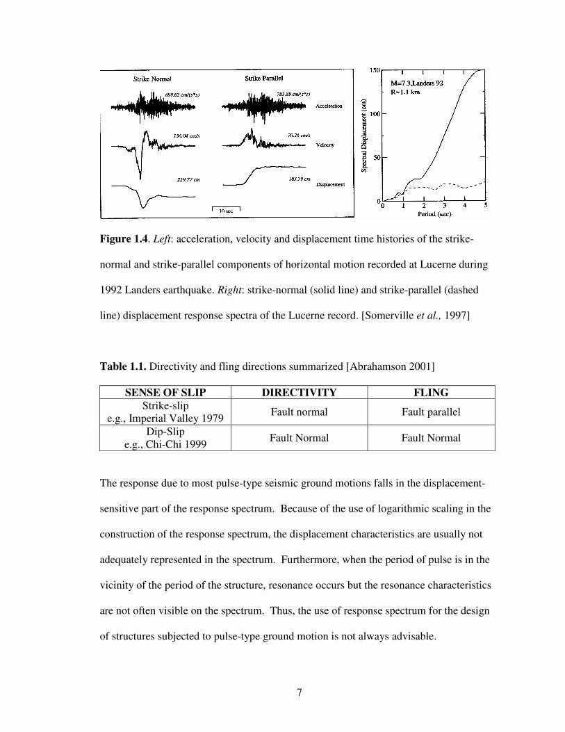
The acceleration, velocity and displacement time histories recorded at Lucerne are shown
in the left part of Fig. 1.4. There is a large difference between the strike-normal and
strike-parallel motions at long periods (velocity and displacement), but this difference
vanishes at short periods (acceleration). The displacement response spectrum of the
strike-normal component greatly exceeds that of strike-parallel component for periods
longer than 1 second, as seen at the right of Fig. 1.4.
7
Figure 1.4. Left: acceleration, velocity and displacement time histories of the strike-
normal and strike-parallel components of horizontal motion recorded at Lucerne during
1992 Landers earthquake. Right: strike-normal (solid line) and strike-parallel (dashed
line) displacement response spectra of the Lucerne record. [Somerville et al., 1997]
Table 1.1. Directivity and fling directions summarized [Abrahamson 2001]
SENSE OF SLIP DIRECTIVITY FLING
Strike-slip
e.g., Imperial Valley 1979 Fault normal Fault parallel
Dip-Slip
e.g., Chi-Chi 1999 Fault Normal Fault Normal
The response due to most pulse-type seismic ground motions falls in the displacement-
sensitive part of the response spectrum. Because of the use of logarithmic scaling in the
construction of the response spectrum, the displacement characteristics are usually not
adequately represented in the spectrum. Furthermore, when the period of pulse is in the
vicinity of the period of the structure, resonance occurs but the resonance characteristics
are not often visible on the spectrum. Thus, the use of response spectrum for the design
of structures subjected to pulse-type ground motion is not always advisable.

8
An important reason why the study of system response to pulse-like near-fault ground
motion (NFGM) is warranted is that these long-period pulses often impose large demands
on structures with relatively long natural periods. When the input time history is a near-
fault pulse, small modifications to this time history can have a major effect on structural
response even though they do not necessarily manifest themselves in the response
spectrum. The response spectrum alone does not provide an adequate characterization of
these pulses because they are relatively simple long-period events with a relatively brief
duration, as opposed to being a stochastic process of relatively long duration.
Furthermore, for Performance Based Design it is crucial that realistic ground motion
inputs and representative models be used to evaluate structure response [Somerville
1998]. A normalized 5%-damped elastic response spectrum for ground motions in fault-
rupture zone has been recently proposed [Goel and Chopra 2008].
1.3 HISTORICAL PERSPECTIVE
The advent of modern digital seismographs has made the recording of seismic ground
motions of relatively low frequencies (i.e., long periods) possible. Such ground motion
records of quakes from the late eighties have provided engineers with useful data to study
the nature of rupture directivity embedded in these ground motions. The effects caused
by rupture directivity are often characterized by the existence of velocity- or acceleration-
pulses in the near-fault ground motions. They are important design considerations
9
because they often impose large displacement demands on medium- to long-period
structures.
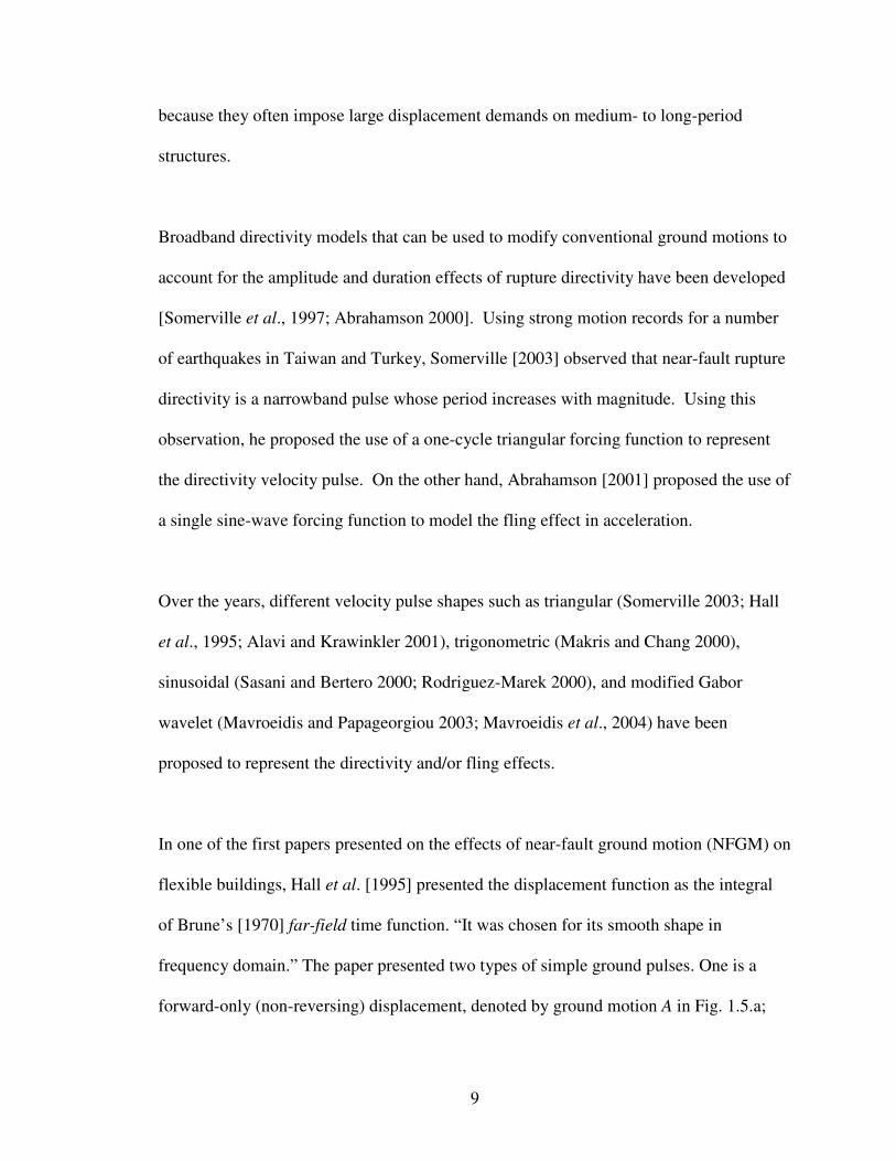
Broadband directivity models that can be used to modify conventional ground motions to
account for the amplitude and duration effects of rupture directivity have been developed
[Somerville et al., 1997; Abrahamson 2000]. Using strong motion records for a number
of earthquakes in Taiwan and Turkey, Somerville [2003] observed that near-fault rupture
directivity is a narrowband pulse whose period increases with magnitude. Using this
observation, he proposed the use of a one-cycle triangular forcing function to represent
the directivity velocity pulse. On the other hand, Abrahamson [2001] proposed the use of
a single sine-wave forcing function to model the fling effect in acceleration.
Over the years, different velocity pulse shapes such as triangular (Somerville 2003; Hall
et al., 1995; Alavi and Krawinkler 2001), trigonometric (Makris and Chang 2000),
sinusoidal (Sasani and Bertero 2000; Rodriguez-Marek 2000), and modified Gabor
wavelet (Mavroeidis and Papageorgiou 2003; Mavroeidis et al., 2004) have been
proposed to represent the directivity and/or fling effects.
In one of the first papers presented on the effects of near-fault ground motion (NFGM) on
flexible buildings, Hall et al. [1995] presented the displacement function as the integral
of Brune’s [1970] far-field time function. “It was chosen for its smooth shape in
frequency domain.” The paper presented two types of simple ground pulses. One is a
forward-only (non-reversing) displacement, denoted by ground motion A in Fig. 1.5.a;

10
the other is a forward-and-back (reversing) displacement, denoted by ground motion B in
Fig. 1.5.b. The duration of displacement-pulse B is Tp, while that of pulse A is Tp/2. The
peak ground displacements and the peak ground velocities were calculated at 121 stations
for a simulated Mw 7.0 earthquake. The period of pulse was related to the fundamental
period of two shear buildings. Their velocity pulses were idealized in triangular form.
Figure 1.5. Velocity pulses idealized in triangular form: Simple pulse-type ground
motions A (forward motion only) and B (forward-and-back motion) [Hall et. al., 1995]
Alavi and Krawinkler [2001] adopted five velocity pulse forms that were best fitted onto
14 different velocity time-histories. These triangular velocity pulses have forms with 0.5,
1, 1.5, 2 and 2.5 cycles of motion.

11

12
Figure 1.6. Triangular velocity pulses from Alavi and Krawinkler [2001]:
Pulse P1 and P2 ground acceleration, velocity and displacement time histories.

13
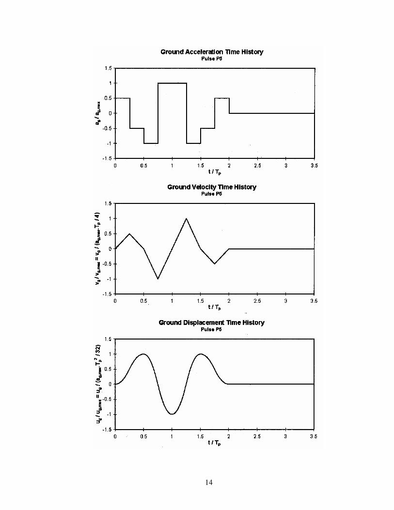
14

15
Figure 1.7. Triangular velocity pulses from Alavi and Krawinkler [2001]: P4, P5 and P3
ground acceleration, velocity and displacement time histories.
16
Pulse type was based on an inspection of the time history trace, and on a comparison
between the ground motion and pulse spectral shapes (primarily velocity and
displacement spectra). The period of pulse, Tp was identified from the location of a global
and clear peak in the velocity response spectrum. The velocity and displacement spectra
of these pulses were superimposed on the velocity and displacement spectra of near-fault
records. The best-fit was adopted. “The objective of the work was not to develop pulses
that can accurately replicate recorded ground motion, but to develop pulses that can
reasonably simulate predominant response characteristics of structures located in the
near-fault regions.”
Makris and Chang [2000] introduced “physically realizable” cycloidal pulses, and
illustrated their resemblance to recorded near-source ground motions. A type-A cycloidal
pulse approximates a forward motion, a type-B cycloid pulse approximates a forward-
and-back motion, whereas, a type-Cn pulse approximates a recorded motion that exhibits
n main pulses in its displacement history. The velocity histories of all type-A, type-B and
type-Cn pulses are differentiable signals that result in finite acceleration values. The best-
fit method of pulse identification was adopted by Makris and Chang (Fig. 1.8).

17
Figure 1.8. Idealized trigonometric pulses by Makris and Chang [2000]. Fault-normal
components of the acceleration, velocity and displacement time histories recorded at the
Rinaldi station during the 1994 Nothridge, earthquake (left), a cycloidal type-A pulse
(center) and a cycloidal type-B (right)
Sasani and Bertero [2000] adopted the best-fit method with simple sinusoidal shapes for
velocity pulses. Rodriguez-Marek [2000] also proposed that near-fault forward-
directivity motions can be adequately represented by simplified time-histories consisting
of one or a few sine-pulses. Later, Lili et al. [2005] proposed four Fling-step pulses
(FSP) and four forward-directivity pulses (FDP), as shown in Fig. 1.9.

18
Figure 1.9. Triangular and sinusoidal simple velocity pulses: Description and
classification [Lili et al., 2005]
Sasani [2006] later proposed an equivalent rectangular acceleration pulse, called the
Significant Peak Ground Acceleration (SPGA). The SPGA is defined as the maximum
ratio of the significant variation of the ground velocity (SVGV) and its duration.
In recent work, Jalali et al. [2007] adopted a very simplified approach, and the pulse is
uniquely adopted as Brune’s pulse, [Brune 1970] which is compared to and calibrated
against fault-slip and recorded ground motions in terms of their peak amplitudes in time
and their spectral contents.
19
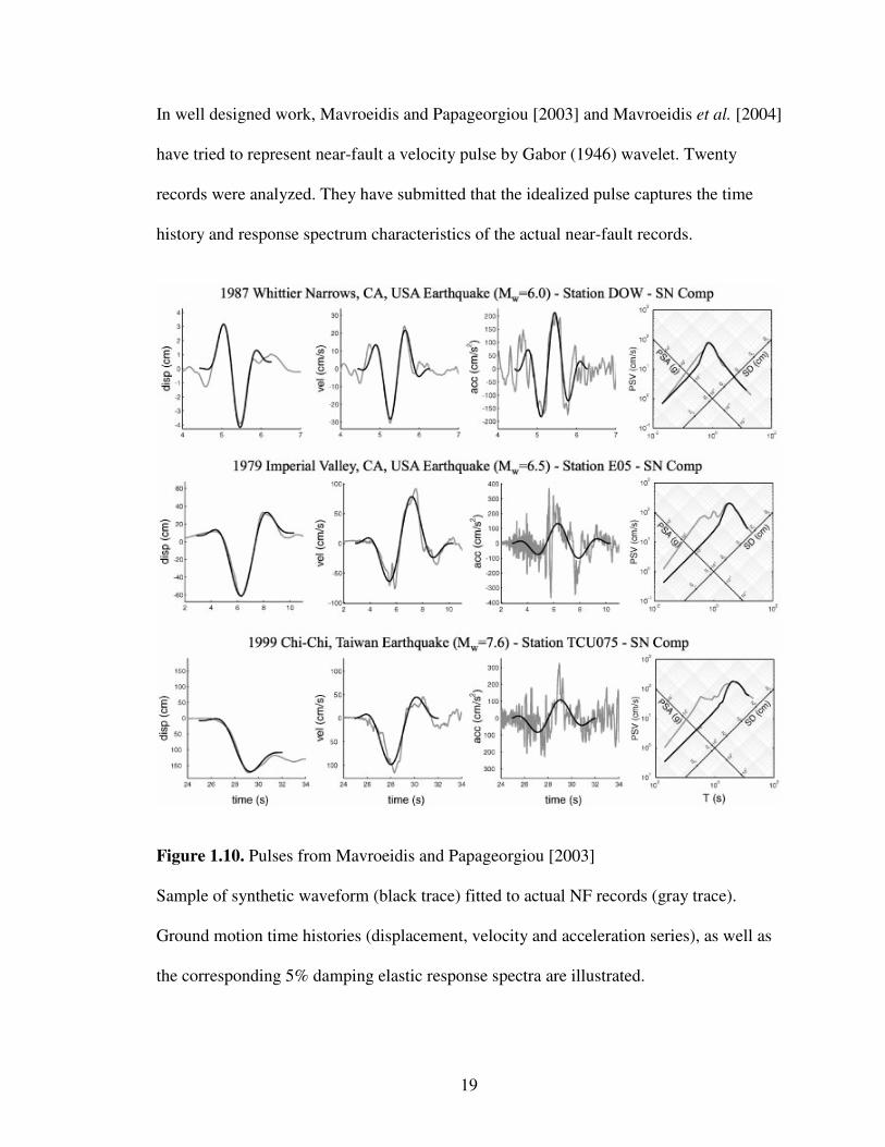
In well designed work, Mavroeidis and Papageorgiou [2003] and Mavroeidis et al. [2004]
have tried to represent near-fault a velocity pulse by Gabor (1946) wavelet. Twenty
records were analyzed. They have submitted that the idealized pulse captures the time
history and response spectrum characteristics of the actual near-fault records.
Figure 1.10. Pulses from Mavroeidis and Papageorgiou [2003]
Sample of synthetic waveform (black trace) fitted to actual NF records (gray trace).
Ground motion time histories (displacement, velocity and acceleration series), as well as
the corresponding 5% damping elastic response spectra are illustrated.

20
Using the Haskell source model and fifty-two NFGM records, Fu and Menon [2004]
proposed a velocity and its corresponding acceleration pulse model based on the synthetic
ground motions generated.
Table 1.2. Summary of research on velocity pulse identification:
No Article Vel. Pulse Shape Characteristics
1 Hall et al. 1995 Triangular A:for forward
displacement.
B: for forward &
backward displacement
2 Somerville 1998 Random -
3 Somerville 2003 Triangular
Narrow band rupture
directivity, 1 cycle
4 Alavi and Krawinkler 2001 Triangular ½, 1, 1.5, 2 & 2.5 cycles
5 Makris and Chang 2000 Trigonometric/
cycloidal
A, B & Cn types
6 Sasani and Bertero 2000 Sinusoidal ½ & 1 cycle, modified
normalized response
spectra
7 Rodrigue-Marek 2000 Sinusoidal 1 or a few cycles
8 Lili et al., 2005 Triangular &
sinusoidal
4 fling & 4 forward
directivity, 1 or ½ cycles
9 Sasani 2006 Rectangular Acceleration, SPGA
10 Jalali et al., 2007 Brune’s pulse -
11 Mavroeidis and Papageorgiou
2003, 04
Modified Gabor
wavelet
Misc.
12 Baker 2007 Daubechies
wavelet of 4th
order
Misc.
A quantitative classification of NFGM using wavelet analysis has been proposed by
Baker [2007]. He proposed the use of a Daubechies wavelet of the fourth order as the
mother wavelet in the wavelet analysis for pulse extraction, since “it approximates the
shape of many velocity-pulses.”

21
The Wave Propagation Method has been proposed by a few researchers to estimate the
displacement demand of structures in near-fault areas. One of the first proposals is by
Hall et al. [1995]. Iwan, W. D. [1997] proposed the use of a Drift Spectrum to measure
the demand for buildings in pure shear subjected to pulse-like NFGM. Miranda and
Akkar [2006] recently developed a generalized interstory drift spectrum that can be
extended to buildings that may deform laterally in flexure, as well as like a shear beams.
There have been case studies on the behavior of 10 to 20-story regular, as well as
irregular steel moment frame buildings subjected to pulse-like near-fault ground motions.
[Alavi and Krawinkler 2001; Kalkan and Kunnath 2006; Krishnan 2007]
1.4 OBJECTIVES AND SCOPE
The major objective of this study was to develop a basic understanding of the
characteristics of pulse-like near-fault ground motions (NFGM) & its impact on response
characteristics of SDF system. The excitation properties intrinsic to pulses are inherently
different from non-pulse type seismic ground motions.
The response due to most pulse-type seismic ground motions falls in the displacement-
sensitive part of the response spectrum. Because of the use of logarithmic scaling in the
construction of the response spectrum, the displacement characteristics are usually not
adequately represented. Furthermore, when the period of the excitation-pulse is close to
the period of the structure, the resonance characteristics are not often visible on the
spectrum even though the displacement dynamic magnification may be quite high. Over

22
the last two decades, very large displacements have been observed for bridge
superstructures, piers and abutments in the near fault area. Recent research has
attributed these large displacements to pulse-like seismic ground motions.
In a seismic design, design for displacement is just as important as the design for forces.
Because different criteria for displacement, strength, and ductility requirements may be
different for pulse-like or non-pulse-like seismic ground motions, in-depth study of
response characteristics of structures subjected to pulse-like ground motion is warranted.
The excitation properties intrinsic to pulses are inherently different from non-pulse type
seismic ground motions. For example, while structural damping does not have an
appreciable effect on the response characteristics of long-period structures when
subjected to non-pulse type ground motions, it greatly affects the response of long-period
structures under pulse-type ground motions. Such pulse-like excitations affect medium-
to long-period structures, often resulting in excessive displacements during the
earthquake or residual displacements after the cessation of earthquake.
In view of this, the study of SDF system subjected to pulse-like NFGM is the subject of
this research work. Because of the limited number of pulse-like seismic ground motion
samples available world-wide (around seventy-five) when compared to the thousands of
seismic ground motion time histories of non-pulse type (regular) seismic ground motions,
a deterministic (as opposed to a probabilistic) approach is used in the present study.
The principal objectives of this dissertation are four-fold:

23
a) MORE REALISTIC PULSE-SHAPES: Most other researchers have assumed a
predetermined pulse shape in the analysis. The principal objective here was to
explore if there is a better way to extract the near-fault velocity pulse/s by using
signal processing techniques that would yield more realistic pulse-shapes.
b) DYNAMIC MAGNIFICATION: The pulse effect of forward rupture directivity
becomes significant at a period of 0.67 sec. and generally grows in size with
increasing period [Somerville et al., 1997]. These responses generally fall within
the displacement-sensitive region of the response spectrum. One of our objectives
was to statistically evaluate the effect of pulses on the dynamic magnification of a
linearly elastic SDF system.
c) ANALOGOUS DISPLACEMENT RESPONSE SPECTRUM: For rupture
directivity and path effects, the lowermost frequency contents of ground motions -
i.e., frequencies between the lowest usable frequency (LUF) and 1.67 Hz - have
been found to play an important role in the displacement response of a single
degree-of-freedom (SDF) system. Because of limitations in instrumentation and
ground motion processing technology, not all frequency records are reliable. The
lowest usable frequency is defined as the lowest recorded frequency that can be
used with confidence for seismic analysis and design. They can be determined
using methods outlined in http://peer.berkeley.edu/nga/NGA_Documentation.pdf.
LUF value for each earthquake record can be found in the PEER NGA Ground
Motion Library. In the time domain, the pulses are visible in the velocity time
history. However, in the frequency domain, the question we would like to have
an answer for is: what information do the Fourier amplitudes convey within this

24
frequency range? This inquiry resulted in the introduction of an analogous
displacement response spectrum for an undamped linearly elastic SDF system.
d) DISPLACEMENT DUCTILITY REQUIREMENT: Herein, we would like to
explore whether the ductility and strength requirements for structures subjected to
pulse-like NFGM are different from those structures subjected to non-pulse type
(regular) seismic ground motions. This objective resulted in the last chapter of
the dissertation, which examines the displacement ductility requirements for a
typical bridge bent subjected to such extreme loadings.
For rupture directivity and path effects, the lowermost frequency contents of ground
motions - i.e., frequencies between the lowest usable frequency (LUF) and 1.67 Hz - of
have been found to play an important role in the displacement response of a single
degree-of-freedom (SDF) system. Using this information, a methodology has been
proposed (see Chapter 2) to identify these effects. An important difference between the
proposed approach and those of the other researchers is that no predetermined pulse
shape is assumed in the analysis. The natural shape and duration of the pulses are
extracted directly from the processed ground motion records. These extracted pulses are
then used to determine their effects on linearly elastic SDF systems.
The pulses can be identified by the use of a discrete-time signal processing method, in
which a low-pass filter with a suitable cut-off frequency is applied to the Fourier
transforms of the processed acceleration or velocity time history records. Chapter 2
discusses the pulse-effects by plotting displacement response spectra computed from the
25
original, pulse and residual acceleration time histories (ATH). By using just the
acceleration pulse as the excitation force, it has been shown that the displacement
response of a linearly elastic SDF system with a natural period exceeding a certain value-
referred to as the cut-off period Tc (the reciprocal of the cut-off frequency fc) –is quite
comparable to the one caused by the original ground excitation.
Qualitatively, the effects of three types of pulses -monotonically increasing, ripple and
resonance -on the system displacement response are identified. Quantitatively, these
three pulse types are identified though a modified displacement response factor Rd (see
Chapter 3). Because the values of Rd can be as high as 10 to 25 for resonant pulses acting
on an undamped SDF system, it can be concluded that such pulses are the most
devastating. A statistical study of the effects of dynamic magnification caused by near-
fault ground motions, using a modified displacement response factor Rd, is presented.
This Rd is used in conjunction with the acceleration pulses extracted event-wise from
pulse-like ground motions to quantify the elastic response characteristics of a system
having damping ratios ζ = 0, 0.02 & 0.05.
The evaluation and examination of the displacement response spectra (DRS) for a
number of near-fault ground motions have led to the observation that they bear a strong
resemblance to the ground velocity Fourier amplitudes. In the low-frequency range (i.e.,
LUF ≤ f ≤ fc < 1.67 Hz), it is observed that the maximum displacement of a linearly
elastic undamped SDF system having a natural period of Tn ≈ Tj (where Tj is the period
corresponding to the jth
harmonic of the earthquake ground motion) is somewhat related

26
to the amplitude of the jth
harmonic ground velocity. Using this information, a method is
introduced in Chapter 4 to allow engineers to construct analogous displacement response
spectra for an undamped linearly elastic SDF system subjected to long-period ground
motions. This spectrum, which is obtained through the transformation of the velocity
Fourier amplitudes (VFA) of the ground velocity time history (VTH), may be used to
determine design ground motions or may be used in Performance-Based Seismic Design
by relating spectral displacements directly to ground velocities via Fourier amplitudes.
In Chapter 5, the dissertation finally examines the ductility requirements for a typical
bridge bent subjected to such pulse-like near-fault ground motions. The ductility
requirement stated in prevailing design codes may not be valid for such structures in
near-fault zones (of less than 10 miles distance). Due to the dominance of the pulses,
medium- to long-period structures are highly affected, which often results in high
residual or permanent deformations after the cessation of seismic ground motions. As per
most design codes, the magnitude of displacements associated with P-Delta effects is
required to be captured using non-linear time history analysis. The higher the value of
the target displacement ductility demand or the P-Delta ratio, the larger is the magnitude
of the residual displacements. Because permanent deformations in a bridge bent would
lead to higher eccentric loading from the superstructure, the bent would be subjected to
higher secondary moments from its own design load. A suitable balance should therefore
be made between ductility and residual displacements in the design of such structures.

27
The scope of this research is limited by the availability of pulse-like acceleration-time-
history samples worldwide as of to-date. At present, only around seventy-five are
available for use in research. This is a very small number when compared to the
availability of non-pulse type (regular) acceleration-time-history samples, which are in
the thousands. These seventy-five records are arranged event-wise in Chapter 3, and
arranged as per seismic moment magnitude and the soil-types in Chapter 5.

28
CHAPTER 2
PULSE IDENTIFICATION AND DISPLACEMENT RESPONSE EVALUATION
2.1 INTRODUCTION
Directivity effects in ground motions can usually be detected in signal processing using
either Wavelet theory or Fourier analysis. While Wavelet theory is more useful when
transitory characteristics or time information is more crucial in the analysis, Fourier
analysis is more appropriate when the frequency contents of the signals are of greater
importance, as in the case of directivity, when a pulse might not be apparent in the
velocity time history (VTH).
In this chapter, an analytical approach for pulse identification and linear displacement
response evaluation in the frequency domain is proposed. The method makes use of
structural dynamics theory [Clough and Penzien 1992; Chopra 2007; Humar 2002], in
conjunction with digital signal-processing techniques [Oppenheim et al. 1999; Mitra
2006], to develop the necessary filter and displacement frequency response functions for
the analysis. An important difference between the proposed approach and those of the
other researchers is that no predetermined pulse shape is assumed. The natural shape and
duration of the pulses are extracted directly from processed ground motion records.
These extracted pulses are then applied to single degree-of-freedom (SDF) systems, so
that their effects can be determined.

29
Although digital filters have been applied to raw records for some time, the proposed
application of low-pass digital filters to processed records for identifying velocity and/or
acceleration pulses is relatively new. In addition, in order to avoid aliasing in the
reconstructed signals, a suitable type and order of filter with an appropriate cut-off
frequency must be used. A procedure for selecting such a filter is also proposed.
According to Somerville et al. [1997], the pulse effect of forward rupture directivity
becomes significant at a period of 0.6 seconds (or at a frequency of 1.67 Hz) and
generally grows in size with the increasing period. For a pulse-like near-fault ground
motion (NFGM), this observation suggests that the cut-off frequency ( fc or c
ω = 2π fc),
defined herein as the frequency above which the Fourier amplitudes are significantly and
continuously lower, can be identified through visual examination of the Fourier
transforms of the ground velocity time history (VTH), measured in the direction of
maximum velocity.
In some cases (Lucerne, TCU068, etc.), applying Fourier analysis to the VTH will yield a
single peak in the Fourier spectra within a frequency range that is defined by the range
from the lowest usable frequency (LUF) to the cut-off frequencyc
f (which should not
exceed 1.67 Hz). This single peak signifies the presence of a dominant single-period
pulse. However, in other cases (such as KJMA, Kobe 1995; HWSM, Imperial Valley-6
1979; CH1, the Loma Prieta 1989 earthquake, etc.) multiple peaks are observed in the
velocity Fourier spectra in the frequency range LUF ≤ f ≤ fc ≤ 1.67 Hz. The presence of
multiple peaks signifies the existence of multiple-period pulses. These pulses will affect

30
the displacement response characteristics of a linearly elastic SDF system at different
natural vibration periods n
T .
In this dissertation, velocity and acceleration pulses are identified by applying a low-pass
discrete-time (digital) filter ( )lp
H ω at a suitable cut-off frequency, fc, to the Fourier
transforms of the ground velocity and acceleration time histories. The linear
displacement response of the extracted acceleration pulse can then be simultaneously
evaluated as the Fourier integral subjected to an arbitrary excitation in the frequency
domain. The proposed procedure is shown schematically in Fig. 2.1.
System Input System Output
( )
uH ω ( ) ( )
uH Pω ω displacement response, ( )u t Eq. (2.4)
Excitation, p(t) ( )lp
H ω ( ) ( )lp
H Pω ω pulse excitation, ( )p
p t Eq. (2.11)
( ) ( )u lp
H Hω ω ( ) ( ) ( )u lp
H H Pω ω ω displacement due to pulse
excitation, ( )p
u t Eq. (2.14)
Figure 2.1. Solution of the linear displacement response to earthquake pulse/s
As shown in the topmost path of Fig. 2.1, the displacement response of a single degree-
of-freedom (SDF) system can be obtained in the frequency domain through modulation
of ( )P ω , defined as the Fourier transform of an excitation function p(t), by a
displacement response function ( )uH ω . Herein, as shown in the middle path of the
figure, it is proposed that a low-pass filter response function ( )lp
H ω be used to modulate

31
( )P ω to obtain an excitation function pp(t) due to the pulse/s. ( )lp
H ω is also used to
identify the acceleration pulse/s ( )p
a t and velocity pulse/s ( )p
v t . Finally, as per the
lowermost path of Fig. 2.1, the displacement response due to the pulse excitation is
obtained by the simultaneous application of ( )uH ω and ( )lp
H ω . In what follows, a more
detailed discussion of each of the aforementioned paths will be given.
By using only the pulse component of the ground motion as the excitation force, it is
shown that the displacement response of a SDF system with a natural period exceeding a
certain value, referred to as the cut-off period c
T , is quite comparable to that caused by
the original ground excitation. Also, for ground motions that contain multiple-period
pulses, it is shown that the displacement response spectrum of the SDF system exhibits
multiple peaks at different natural system periodsn
T .
2.2 EXCITATION AND ITS RESPONSE IN THE FREQUENCY DOMAIN
The equation of motion for a SDF damped system subjected to an excitation force ( )p t is
given by [Clough and Penzien 1992; Chopra 2007; Humar 2002]
( )mu cu ku p t+ + =&& & (2.1)
where m is the mass, c is the viscous damping coefficient, k is the stiffness, and ( )u t ,
( )u t& and ( )u t&& are the resulting time-dependent displacement, velocity and acceleration of
the system, respectively.
If we express the excitation force p(t) as

32
1
( ) ( )2
i tp t P e d
ωω ωπ
∞
−∞
= ∫ (2.2)
where
( ) ( ) -i tP p t e dt
ωω∞
−∞
= ∫ (2.3)
in which 1= −i and ω is the forcing frequency in radians/second, the response of the
system can be obtained as
1
( ) ( )2
i tu t U e d
ωω ωπ
∞
−∞
= ∫ (2.4)
where
( ) ( ) ( )u
U H Pω ω ω= (2.5)
and
( ) ( )
2
1 1( ) ( / )
1 / 2 /u u n
n n
H Hk
ω ω ωω ω ζ ω ω
= = × − +
i (2.6)
in which /n
k mω = is the natural frequency, and / 2n
c mζ ω= is the damping ratio of
the SDF system. It may be observed that ( )u
H ω modulates the frequencies by
convoluting with the input ( )p t to yield the linear displacement response ( )u t .
2.3 LOW-PASS FILTER RESPONSE FUNCTION, ( )lp
H ω
2.3.1 DIGITAL FILTERS
Frequency-selective filter implies a system that passes certain frequency components and
totally rejects all others, however, broadly it is any system that modulates certain
frequencies relative to others [Oppenheim et al., 1999].

33
Digital filters may be broadly classified into:
1. Discrete-time Infinite Impulse Response (IIR) filters designed from continuous-
time filters, e.g., the Butterworth filter, the Chebyshev filter, etc.
2. Finite Impulse Response (FIR) filters (linear phase) designed by ‘windowing’,
e.g., rectangular, Bartlet, Hanning, Hamming, Blackman, Kaiser etc.
3. FIR filters (nonlinear phase) designed by optimization algorithms like the Parks-
McClellan algorithm, e. g., Equiripple filters.
Let the sampling interval be t∆ and N the total number of sampling points of the record.
Then the sampling ratio, SR, is equal to 1/ t∆ . To avoid ‘aliasing’, the number of Fourier
Transform (FT) points should be equal to or more than the number of sampling points. If
these are fewer than the sampling points, the original time history is not recoverable;
there is a distortion referred to as aliasing distortion, or simply, aliasing. Typical required
low-pass specifications of ( )lp
H ω are depicted in Fig. 2.2., where the limits of tolerable
approximation errors are 1δ and 2δ for passband and stopband, respectively. p
ω and
sω are the passband frequency and the stopband frequency, respectively. Passband is that
band of a spectrum, which frequencies are allowed to pass through (retained). The
frequencies in stopband are discarded. Only in the case of an ideal low-pass filter is the
transition band width zero, as stated in the following section 2.3.2. The transition band is
required to avoid aliasing distortions while reconstructing the modulated signals. The
width of the transition band depends upon the type and order of the filter used.

34
The purpose of following two sections is to introduce two simple filters and to show how
the frequency response function of filter ( )lp
H ω plays an important role in modulating
frequencies.
Figure 2.2. For the low-pass filter, specifications for the effective frequency response of
the overall system. [Oppenheim et al., 1999]
2.3.2 IDEAL LOW-PASS FILTER:
Let the system response to ideal low-pass filter be
1
( )0
c
lp
c
Hω ω
ωω ω π
<=
< ≤
where c
ω is the lowpass cut-off frequency in radians per second. In this case,
p s cω ω ω= =
The corresponding discrete impulse response is, [ ]sin
- clp
nh n n
n
ω
π= ∞ < < ∞

35
An ideal low-pass filter should not be applied to “real” input systems, since it gives rise
to aliasing distortions.
2.3.3 BUTTERWORTH LOW-PASS FILTER [Oppenheim et al., 1999]
Although numerous low-pass filters are available in the literature, Butterworth low-pass
filters will be used for the present study. Butterworth low-pass filters are characterized
by the property that the magnitude response is maximally flat in the passband, and that
the magnitude response is monotonic in both the passband and stopband. In particular,
the continuous-time Butterworth low-pass filter is expressed as
( )
1( )
1 /iB
lp N
c
H ωω ω
=+
(2.7)
where 1= −i , c
ω is the desired cut-off frequency in radians/second, and B
N is the
order of Butterworth filter. The corresponding magnitude-squared function is,
( )
2
2
1( )
1 / Blp N
c
H ωω ω
=+
(2.8)
A plot of ( )lp
H ω versus /c
ω ω is given in Fig. 2.3. Note that asB
N increases, the filter
characteristics become sharper, although the magnitude-squared functions at the cut-off
frequency c
ω will always equal one-half because of the nature of Eq. (2.8). AnB
N value
of 32 is used in the current study because, as indicated in the figure, the transition band
becomes extremely narrow at this value. It should also be noted that while “low-cut” and
“high-cut” Butterworth filters are often used to process raw earthquake records to

36
eliminate the lowest and uppermost unwanted frequencies, this low-pass Butterworth
filter retains all frequencies lower than c
ω , but eliminates all frequencies higher than c
ω .
Figure 2.3. Effect of NB on Butterworth low-pass filter magnitude.
2.4 PULSE IDENTIFICATION AND
CUT-OFF FREQUENCY DETERMINATION
For directivity or path effect to be dominant, the peak ground velocity (PGV) in the
direction of maximum velocity is usually larger than 30 cm/s [Baker 2007]. In this study,
digital filters are applied to ground motion time history responses to identify the pulse/s.
If we denote ( )A ω and ( )V ω as the Fourier transforms of the ground acceleration ( )a t
and velocity ( )v t time histories, respectively, the following equations are proposed for
the computation of time histories for acceleration and velocity pulses:
1
( ) ( ) ( )2
i t
p lpa t H A e d
ωω ω ωπ
∞
−∞
= ∫ (2.9)
NB = 4
NB = 8
NB = 16
NB = 32
( )lp
H ω
ω/ωc

37
1
( ) ( ) ( )2
i t
p lpv t H V e d
ωω ω ωπ
∞
−∞
= ∫ (2.10)
In the above equations, ( )lp
H ω is the low-pass Butterworth filter function given by Eq.
(2.7). Similarly, the time history for pulse excitation due to ground motion ( ) ( )p t ma t= −
can be obtained using
1
( ) ( ) ( )2
i t
p lpp t H P e d
ωω ω ωπ
∞
−∞
= ∫ (2.11)
where ( )P ω is the Fourier transform of ( )p t given by Eq. (2.3).
Because directivity effects are most significant for frequencies less than 1.67 Hz (i.e., a
period longer than 0.6 seconds), this criterion is used in the present study to identify the
pulse characteristics. Based on a study of about seventy pulse-like ground motion
records, the following procedure is proposed to determine the cut-off frequency to be
used in Eq. (2.7).
1. For a given set of horizontal ground motion acceleration data recorded at a specified
station, compute the component of the quake in the direction of maximum velocity.
For a strike-slip faulting mechanism, this component is generally in the fault-
normal (FN) direction.
2. Numerically integrate the ground acceleration time history obtained in (1) to obtain
the velocity time history.
3. Perform a Fourier analysis on the velocity time history to obtain the velocity
Fourier spectrum.

38
4. Identify high amplitude spikes in the velocity Fourier spectrum within the window
of frequencies ranging from the Lowest Usable Frequency (LUF), as given in the
ground motion data source, to 1.67 Hz.
5. Determine the cut-off frequency (fc or c
ω ) inside the aforementioned frequency
window as the frequency above which the velocity Fourier amplitudes will become
significantly and continuously lower.
The following examples are used to demonstrate the application of the above procedure.
Example 1 – The Fault-normal component of Nishi-Akashi, Kobe 1995 earthquake
For this record, no velocity pulse is present in the velocity time history (VTH). To verify
this, the velocity Fourier spectrum for the fault-normal (FN) component of this
earthquake at the Nishi-Akashi station was computed and plotted and is shown in Fig.
2.4. Because of the existence of high amplitude spikes beyond the 1.67 Hz frequency
range (i.e., outside of the frequency range of interest), it can be concluded that no pulse
exists for this ground motion. The absence of directivity has been confirmed by
Mavroeidis and Papageorgiou [2003] and Mavroeidis et al. [2004] although Nishi-Akashi
is only 7.08 km away from the fault rupture.
Although directivity effects might not be present, this record (soil type B) has dominant
site effects, as is evident from the presence of high, steep and narrow spikes in the
velocity Fourier spectra for frequencies lower than 2.5 Hz.
39
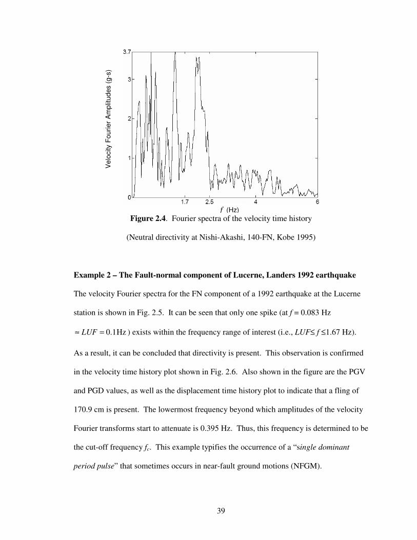
Figure 2.4. Fourier spectra of the velocity time history
(Neutral directivity at Nishi-Akashi, 140-FN, Kobe 1995)
Example 2 – The Fault-normal component of Lucerne, Landers 1992 earthquake
The velocity Fourier spectra for the FN component of a 1992 earthquake at the Lucerne
station is shown in Fig. 2.5. It can be seen that only one spike (at f = 0.083 Hz
0.1HzLUF≈ = ) exists within the frequency range of interest (i.e., LUF≤ f ≤1.67 Hz).
As a result, it can be concluded that directivity is present. This observation is confirmed
in the velocity time history plot shown in Fig. 2.6. Also shown in the figure are the PGV
and PGD values, as well as the displacement time history plot to indicate that a fling of
170.9 cm is present. The lowermost frequency beyond which amplitudes of the velocity
Fourier transforms start to attenuate is 0.395 Hz. Thus, this frequency is determined to be
the cut-off frequency fc. This example typifies the occurrence of a “single dominant
period pulse” that sometimes occurs in near-fault ground motions (NFGM).
f (Hz)
Velo
city F
ourier
Am
plit
ud
es (
g-s
)

40
Ve
locity (
cm
/s),
Dis
pla
ce
me
nt (c
m)
Time (sec)
Figure 2.5. Fourier spectra of the velocity time history showing a single peak
(Single-period pulse at Lucerne, 239-FN, Landers 1992)
Figure 2.6. Velocity and displacement time histories
(Single-period pulse at Lucerne, 239-FN, Landers 1992)
Velo
city F
ourier
Am
plit
ud
es (
g-s
)
f (Hz)
f = 0.083 Hz
fc =0.395 Hz
PGD= 236.0 cm
Fling = 170.9 cm
PGV= 136.1 cm/s
Velo
city (
cm
/s),
Dis
pla
ce
ment
(cm
)

41
Example 3 – The Fault-normal component of the Westmorland Fire Station,
Imperial Valley-6 1979 earthquake
The velocity Fourier spectra for the FN component of this earthquake at the Westmorland
Fire Station is shown in Fig. 2.7. It can be seen that two spikes (at f = 0.1 Hz and 0.225
Hz) exist within the frequency range of interest (i.e., LUF=0.1 Hz ≤ f ≤ 1.67 Hz). The
lowermost frequency beyond which the velocity Fourier amplitudes start to attenuate is
0.475 Hz. This frequency is therefore identified as the cut-off frequency fc. This
example is used to show the existence of two dominant spikes in the velocity Fourier
spectra, which correspond to the two distinct peaks in the displacement response spectra
at Tn ≈ 4.7 sec and 9.5 sec (see Fig. 2.13).
Figure 2.7. Fourier spectra of velocity time history showing multiple peaks
(Multiple-period pulses at the Westmorland Fire Station (HWSM),
233-FN, Imperial Valley-6 1979)
f (Hz)
Velo
city F
ourier
Am
plit
ud
es (
g-s
)
f = 0.225 Hz
fc = 0.475 Hz

42
2.5 PULSE RESPONSE EVALUATION
If we decompose the ground motion into its pulse and non-pulse components, i.e.,
)()()()()( tmatmatptptp nppnpp −−=+= (2.12)
where ( )p
a t is the acceleration associated with the pulse given by Eq. (2.9), and ( )np
a t is
the residual acceleration (i.e., the acceleration excluding the pulse), the displacement
response that corresponds to the pulse component ( ) ( )p p
p t ma t= − can be evaluated
using
1
( ) ( ) ( )2
i t
p u pu t H P e d
ωω ω ωπ
∞
−∞
= ∫ (2.13)
Since ( ) ( ) ( )p lp
P H Pω ω ω= and realizing that ( )u
H ω and ( )lp
H ω are essentially
functions of ( / )n
ω ω and ( / )c
ω ω , respectively, Eq. (2.13) can be written as
( ) ( )1
( ) / / ( )2
i t
p u n lp cu t H H P e d
ωω ω ω ω ω ωπ
∞
−∞
= ∫ (2.14)
where ( / )u n
H ω ω , ( / )lp c
H ω ω , and ( )P ω are given by Eqs. (2.6), (2.7), and (2.3),
respectively.
On the other hand, the displacement response that corresponds to the non-pulse
component of the excitation )()( tmatp npnp −= can be evaluated using
( ) ( )1
( ) / / ( )2
i t
np u n hp cu t H H P e d
ωω ω ω ω ω ωπ
∞
−∞
= ∫ (2.15)

43
where ( / )u n
H ω ω and ( )P ω are defined as before, and ( )hp
H ω is the Butterworth high-pass
filter given by
( ) ( )
( / )1( ) 1 ( ) 1
1 / /i i
B
B B
N
chp lp N N
c c
H Hω ω
ω ωω ω ω ω
= − = − =+ −
(2.16)
It should be noted that this high-pass filter retains frequencies higher than the cut-off
frequency (fc or c
ω ) and discards frequencies lower than the cut-off frequency. Thus, the
application of this filter to the original system response would yield system response
excluding the pulse-effect.
By evaluating and plotting ( )u t , ( )p
u t and ( )np
u t on the same graph, one can compare
and observe the displacement response characteristics for SDF systems having different
natural periods. This comparison will be performed in the following section.
Because ground motion is intrinsically random in nature, all the aforementioned Fourier
integrals have to be performed numerically. For instance, to compute displacement
response given in Eq. (2.14), the following discretized form of the equation is used
( ) ( ) ( ) ( ) ( )1 1
i( ) i(2 / )
0 0
j n
N Nt nj N
p u lp j u lp jj jn j jj j
u H H P e H H P eω π
− −
= =
= =∑ ∑ (2.17)
where N is the total number of samples (i.e., the number of recorded data points), and
( ) ( )2
1 1( )
1 / 2 /u j
j n j n
Hk
ωω ω ζ ω ω
= × − +
i (2.18)
is the discretized form of Eq. (2.6).
( )1
( )1 /
Blp j N
j c
H ωω ω
=+ i
(2.19)

44
is the discretized form of Eq. (2.7), and
1 1
( ) (2 / )
0 00
1 1j n
N Nt nj N
j n n
n n
P p e t p eT N
ω π− −
− −
= =
= ∆ =∑ ∑i i (2.20)
is the discretized form of Eq. (2.3).
The ( )j
H ω values in Eqs. (2.18) and (2.19) are determined with the following
interpretation ofj
ω :
0
0
0 /2
-( - ) /2 -1j
j j N
N j N j N
ωω
ω
≤ ≤=
≤ ≤ (2.21)
In the above equation, 0 02 /Tω π= is the fundamental frequency and j
ω is the frequency
of the jth harmonic. To avoid aliasing, the highest frequency that needs to be used in a
Fourier analysis, known as the Nyquist or folding frequency, is denoted as
max 0 ( / 2) /N tω ω π= = ∆ , where 0 /t T N∆ = . The shortest and longest periods of the
harmonics included in the Fourier expansion are thus determined to be 2 t∆ and T0,
respectively.
Similarly, Eqs. (2.9) and (2.10) are evaluated using the following discretized forms:
( ) ( ) ( )1 1
2 /
0 0
( ) ( )j n
N Nt nj N
p lp j j lp j jnj j
a H A e H A eω πω ω
− −
= =
= =∑ ∑i i
(2.22)
( ) ( ) ( )1 1
2 /
0 0
( ) ( )j n
N Nt nj N
p lp j j lp j jnj j
v H V e H V eω πω ω
− −
= =
= =∑ ∑i i
(2.23)
with the complex Fourier coefficients Aj and Vj computed from
1 1
( ) (2 / )
0 00
1 1j n
N Nt nj N
j n n
n n
A a e t a eT N
ω π− −
− −
= =
= ∆ =∑ ∑i i (2.24)
and

45
1 1
( ) (2 / )
0 00
1 1j n
N Nt nj N
j n n
n n
V v e t v eT N
ω π− −
− −
= =
= ∆ =∑ ∑i i (2.25)
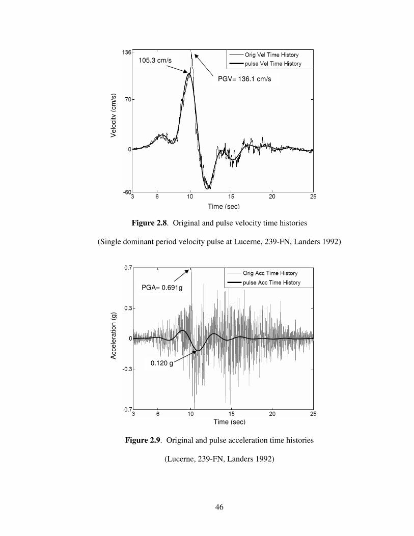
2.6 PULSE EFFECTS
From a study of more than seventy pulse-like ground motions, it has been observed that
the so-called velocity and acceleration pulses are merely dominant low-frequency
sinusoidal waves that occur in the lower-most range of the Fourier spectra. Although
these pulses are sometimes identifiable from the ground velocity time history, they are
not so apparent in the ground acceleration time history. In near-fault areas, they manifest
themselves as directivity effect, whereas in the far-fault areas they manifest as path effect.
In Fig. 2.8, the velocity pulse from the Lucerne 239-FN, Landers 1992 earthquake
(Mw=7.28) obtained using Eq. (2.23) is superimposed on the original ground velocity
time history to show that it consists of a single dominant wave, as confirmed by other
researchers. However, in Fig. 2.9 it can be seen that the acceleration pulse obtained using
Eq. (2.22) is not so visible in the ground acceleration time history.
46
Time (sec)
Time (sec)
Figure 2.8. Original and pulse velocity time histories
(Single dominant period velocity pulse at Lucerne, 239-FN, Landers 1992)
Figure 2.9. Original and pulse acceleration time histories
(Lucerne, 239-FN, Landers 1992)
105.3 cm/s
PGV= 136.1 cm/s
Velo
city (
cm
/s)
PGA= 0.691g
0.120 g
Accele
ratio
n (
g)
47
Time (sec)
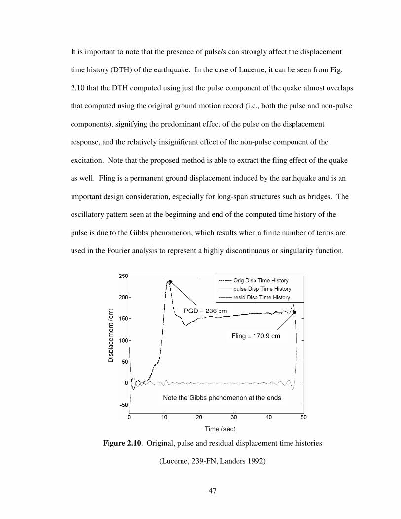
It is important to note that the presence of pulse/s can strongly affect the displacement
time history (DTH) of the earthquake. In the case of Lucerne, it can be seen from Fig.
2.10 that the DTH computed using just the pulse component of the quake almost overlaps
that computed using the original ground motion record (i.e., both the pulse and non-pulse
components), signifying the predominant effect of the pulse on the displacement
response, and the relatively insignificant effect of the non-pulse component of the
excitation. Note that the proposed method is able to extract the fling effect of the quake
as well. Fling is a permanent ground displacement induced by the earthquake and is an
important design consideration, especially for long-span structures such as bridges. The
oscillatory pattern seen at the beginning and end of the computed time history of the
pulse is due to the Gibbs phenomenon, which results when a finite number of terms are
used in the Fourier analysis to represent a highly discontinuous or singularity function.
Figure 2.10. Original, pulse and residual displacement time histories
(Lucerne, 239-FN, Landers 1992)
Fling = 170.9 cm
PGD = 236 cm
Note the Gibbs phenomenon at the ends
Dis
pla
cem
ent
(cm
)

48
Natural period, Tn (sec)
Fig. 2.11 shows the spectral displacements for a linearly elastic SDF system computed
using the original, pulse and non-pulse components of the ground acceleration time
history (ATH), for two damping ratios (ζ=0 and 0.05). Although the peak amplitude of
the acceleration pulse (0.120 g), as indicated in Fig. 2.9, seems rather small when
compared to that of the original ATH, it can be seen that, regardless of the value of ζ, the
spectral displacements computed using just the pulse ATH and the original ATH are
quite comparable when the period of the SDF system is longer than the cut-off period Tc,
which is equal to 2.5 sec. for this record. This indicates that the displacement response of
a SDF system can be determined with a relatively high degree of accuracy by using just
the extracted acceleration pulse provided that the system period is longer than Tc.
Figure 2.11. Displacement response spectra computed from the original, pulse and
residual acceleration time histories (Lucerne, 239-FN, Landers 1992, ζ = 0 and 0.05)
Because no predetermined pulse duration or wave form is used to represent the pulse, an
important feature of the proposed method is its ability to extract multiple-period pulses
ζ=0
ζ=0
ζ=0
ζ=0.05
ζ=0.05
ζ=0.05
pulse Tc = 2.5 s
Spectr
al d
ispla
cem
ents
(cm
) ζ = 0
ζ=0.05
resid, ζ = 0 & 0.05

49
Time (sec)
from long-period ground motions. An example is the Westmorland Fire Station
(HWSM) 233-FN Imperial Valley-6 1979 earthquake (Mw=6.53). Using a cut-off
frequency of fc=0.475 Hz, as shown in Fig. 2.7, the acceleration pulses are extracted as
depicted in Fig. 2.12, and the corresponding spectral displacements for two damping
ratios (ζ = 0 and 0.05) are plotted, as shown in Fig. 2.13. It can readily be seen from the
figure that the spectral displacements dominantly peaked at two locations at n
T ≈ 4.7 sec
and 9.5 sec, which correspond to the two pulses. Furthermore, the spectral displacements
are very comparable regardless of whether they are computed from the original or the
pulse ATH, again signifying the predominant effect of the pulses on the system response.
Figure 2.12. Original and multiple-period pulse acceleration time histories
(Westmorland Fire Station (HWSM), 233FN, Imperial Valley-6 1979 earthquake)
Accele
ratio
n (
g)
(cm
/s)

50
Natural Period, Tn (sec)
Figure 2.13. Displacement response spectra computed from the original, pulse and
residual acceleration time histories (Westmorland Fire Station (HWSM),
233-FN, Imperial Valley-6 1979 earthquake, ζ = 0 and 0.05.)
Finally, as an example of the path effect, the ground motion record for the Oakland -
Outer Harbor Wharf (CH1), 038-FN, Loma Prieta 1989 earthquake (Mw = 6.93) is shown
in Fig. 2.14, along with the extracted acceleration pulses. The corresponding spectral
displacements, calculated using two damping ratios, are given in Fig. 2.15. The
similarity of the spectral displacements computed using just the pulse ATH and the
original ATH is again observed. This station is located at a distance of 74.26 km (46.14
miles) from the fault-rupture. Far-source ground motions consist of surface waves that
sometimes have longer durations than those of the near-fault ones. They can be very
damaging in certain circumstances. This example shows that the proposed approach for
acceleration pulse extraction can be used for both directivity and path effects in
evaluating response characteristics, since long-period ground motions are dominant in
both the cases.
ζ=0
ζ=0
ζ=0
ζ=.05
ζ=.05
ζ=.05
Spectr
al d
ispla
cem
ents
(cm
)
resid, ζ = 0 & 0.05
ζ = 0
ζ = 0.05

51
Figure 2.14. Original and multiple-period pulse acceleration time histories
(Oakland - Outer Harbor Wharf (CH1), 038-FN, Loma Prieta 1989 earthquake)
Figure 2.15. Displacement response spectra computed from the original, pulse and
residual Acceleration time histories, (Oakland - Outer Harbor Wharf (CH1), 038-FN,
Loma Prieta 1989 earthquake, ζ = 0 and 0.05)
0.106 g
Accele
ratio
n (
g)
Time (sec)
Natural Period, Tn (sec)
Spectr
al d
ispla
cem
ents
(cm
)
ζ=0
ζ=0
ζ=0
ζ=0.05
ζ=0.05
ζ=0.05
resid, ζ = 0 & 0.05
ζ = 0
ζ = 0.05

52
2.7 DISCUSSION AND OBSERVATIONS
Based on the above examples, the investigation of the response of an elastic SDF system
to long-period ground motions has led to the following observations:
1. The spectral displacement of a SDF system due to acceleration pulse excitation is
very comparable to that caused by the original acceleration time history excitation
when the period of the SDF system is equal to or higher than the cut-off period c
T ,
which is equal to the reciprocal of the cut-off frequency c
f .
2. This study reaffirms the common observation that long-period structures are
strongly affected by pulse-like long-period ground motions. This is because large
displacements are observed in all these displacement spectra.
3. A single peak in the velocity Fourier spectrum corresponds to the presence of a
single-period pulse, whereas multiple peaks in the lower frequency range of Fourier
spectrum correspond to the existence of multiple-period pulses. Multiple-period
pulses have the potential to significantly affect the displacement response of a
linearly elastic SDF system at different natural periods n
T , or a multi-degree-of-
freedom system with multiple natural periods.
4. From Figs. 2.11, 2.13 and 2.15 in which spectral displacements are shown for two
values of damping ratios (ζ = 0 and 0.05), it can be seen that damping plays an
important role in extenuating the displacement response of the system, even in the

53
displacement-sensitive part of the spectra (i.e., for the natural period of vibration
nT > 0.63 s).
5. From Figs. 2.11, 2.13 and 2.15, it can be seen that the spectral displacement
response for the non-pulse component of the ground excitations does not appear to
change noticeably with damping. This observation supports the general notion that
the effect of damping is not apparent for long-period structures subjected to short-
period (high frequency) excitations.
6. While some NFGM records with a predominant single-period pulse – in cases such
as Lucerne, Landers 1992 – have the distinct characteristic that the spectral
displacements (Fig. 2.11) increase more or less monotonically from the cut-off
period c
T almost to the Highest Usable Period (equal to the reciprocal of Lowest
Usable Frequency as given in the ground motion data source), most records with
multiple periods – such as the Westmorland Fire Station, Imperial Valley-6 1979
(Fig. 2.13) and Oakland – Outer Harbor Wharf, Loma Prieta 1989 (Fig. 2.15) –
show spectral displacements that often exhibit a ripple effect over a wider range of
natural periods that are higher than c
T . Since c
T in some cases may be from 0.6 to
1.0 second, even medium-period structures may be affected by such ground
motions. It is important to note that these two characterizations are not apparent
when conventional tripartite response spectra are used.
54
2.8 PARSEVAL’S THEOREM AND PULSE ENERGY
In this section, the energy associated with the pulses is computed using Parseval’s
theorem [Mitra 2006] to demonstrate that these pulses contribute a considerable amount
of energy to the total seismic energy of a long-period ground motion.
If we denote x(t) as the amplitude of a signal in the time domain and X(ω) as the Fourier
transform of x(t), the simplified version of Parseval’s theorem states that the total energy
of the signal can be computed from the following relationship
( ) ( )2 21
2x t dt X dω ω
π
∞ ∞
−∞ −∞
=∫ ∫ (2.26)
In discretized form, the above equation can be written as
[ ] [ ]1 1
2 2
0 0
1N N
n k
x n X kN
− −
= =
=∑ ∑ (2.27)
This equation can be used to evaluate the energy of the pulses if we set [ ] [ ]x n v n=
and [ ]0[ ]X k V kω= , where [ ]v n and [ ]0V kω are the velocity time history and its Fourier
transforms, respectively. The calculated ratios of energy generated by the velocity
pulse/s to that generated by the entire velocity time history are 0.952, 0.952 and 0.701 for
the Lucerne 239-FN (near-fault), Westmorland Fire Station 233-FN (near-fault), and
Oakland –Outer Harbor Wharf 038-FN (far-fault) ground motions, respectively. Thus, it
is observed that these velocity pulses carry quite a large percentage of the total seismic
energy generated from the rupture.

55
2.9 SUMMARY AND CONCLUSIONS
In this chapter a procedure for identifying velocity and acceleration pulses for near-fault
ground motion records was proposed. The procedure involves the application a Fourier
analysis to the velocity time history in the direction of maximum velocity, which is
generally fault-normal (FN) for a strike-slip faulting mechanism.
Single- and multiple-period pulses are identified as the existence of one or more large
amplitude spikes in the velocity Fourier spectrum within the frequency range of LUF to
1.67 Hz, where LUF is the lowest usable frequency as specified in the ground motion
data source. For the present research, all the ground motion records were accessed from
PEER NGA data source. Once these pulses are identified, the cut-off frequency is
determined as the lowest frequency on the Fourier spectrum above which the Fourier
amplitudes will attenuate. The cut-off period is then computed as the reciprocal of this
cut-off frequency.
Using this cut-off frequency as input to a Butterworth low-pass filter, Fourier integral and
discretized equations capable of extracting acceleration and velocity pulses from the
original ground motion records were proposed. An analytical equation for computing the
displacement response of a SDF system subjected to these pulses was also presented.
Examples were given to demonstrate the validity of the proposed procedure.
Furthermore, the Parseval Theorem was used to compute the amount of seismic energy
generated by these pulses.
56
Based on the results of this study, the following conclusions can be drawn:
1. Frequencies less than 1.67 Hz play a vital role in pulse-like near-fault ground
motions (NFGM). Because for most pulse-type NFGM records, the velocity
Fourier amplitudes for frequencies lower than 1.67 Hz are often more dominant
than those for frequencies higher than 1.67 Hz, this observation has been used in
the proposed procedure for pulse identification.
2. Long-period (low-frequency contents) pulse-like ground motions can significantly
affect the relevant displacement characteristics of SDF systems.
3. When the pulse displacement time history (DTH) that corresponds to the pulse/s
is plotted with the original DTH, they almost overlap. This demonstrates the
predominant effect of long-period ground motions on DTH.
4. Because most pulse-like NFGM consist of multiple period pulses, representation
of the pulse by characterizing it as a single-period wave-form with a specific
duration may be unrealistic in most cases.
5. Spectral displacement plots of pulse-like NFGM at different damping ratios have
shown that the displacement responses due to the identified pulse/s are very
comparable to those caused by the original excitations when the fundamental
period of the system is longer than its cut-off period c
T , which is defined as the
reciprocal of the cut-off frequency fc.
6. The energy associated with the pulse/s computed using Parseval’s theorem shows
that a considerable amount of the total seismic energy is due to this/these pulse/s.
57
7. Since the displacement response has been evaluated in the frequency-domain, the
application is theoretically restricted only to linearly elastic systems. However,
the identified and extracted pulse/s can be used in the time-domain for both linear
and nonlinear seismic demand computations.
Thus, in this chapter we have extracted acceleration/velocity pulse/s from the original
acceleration time history by discrete-time signaling process using low-pass Butterworth
filter with suitable a cut-off frequency. We have further demonstrated that by using only
the pulse component of the ground motion as the excitation force, the displacement
response of the SDF system with a natural period exceeding a certain value referred to as
the cut-off period c
T , is quite comparable to that caused by the original ground excitation.
Because most NFGM consist of multiple-period pulses, representation of the pulse by
characterizing it as a single-period wave-form with a specific duration may be unrealistic
in most cases. In the next chapter we will proceed to demonstrate this. We will also
proceed to study the qualitative and quantitative nature of pulses, and evaluate the
modified displacement response factor event-wise.

58
CHAPTER 3
Modified Displacement Response Factor, Rd (Dynamic Magnification Factor)
3.1 INTRODUCTION AND OVERVIEW
Long-period near-fault ground motions (NFGMs) occur as a result of the source effects
of rupture directivity. Because of path effects, large subduction-zone earthquakes, as
well as moderate to large crustal earthquakes, can generate far-source long-period ground
motions in distant sedimentary basins. These effects are important design considerations
because they often impose large demands on medium- to long-period structures.
As elaborated in Chapter 2, a discrete-time signal processing method was proposed to
isolate the low-frequency contents of processed ground motions, from which velocity and
acceleration pulses were identified after application of low-pass discrete-time (digital)
filter ( )lpH ω , at a suitable cut-off frequency, fc, to the Fourier transforms of their
respective time histories. By using the acceleration pulse as the excitation force, it was
also shown that the displacement response of a linearly elastic single degree-of-freedom
(SDF) system with natural period exceeding a certain value, referred to as the cut-off
period, is quite comparable with that caused by the original ground excitation. A brief
review of the procedure will be given in Sec. 3.2.

59
In this chapter 3, the displacement response characteristics of a linearly elastic SDF
system subjected to pulse-like excitation is studied qualitatively and quantitatively.
Qualitatively, three types of pulse effects are identified:
(1) Monotonically increasing displacement: The spectral displacements increase
more or less monotonically with the natural period n
T of the structure. This
generally occurs when the acceleration pulse has a single predominant period. (i.
e., a single predominant frequency peak in the Fourier spectrum, in the frequency
range LUF ≤ f ≤ fc ≤ 1.67 Hz).
(2) Ripple effect: The spectral displacement peaks at different natural periods. This
generally occurs for multiple-period pulses (multiple frequency peaks in Fourier
spectrum in the said frequency range)
(3) Resonance effect: This is a special case of multiple-period pulses in which the
spectral displacements are very high compared to their static counterparts. In the
velocity Fourier spectrum, these are apparent as high and steep (high gradient)
Fourier amplitudes.
To quantitatively identify these three types of pulse effects, the concept of a modified
displacement response factor d
R is introduced. Based on the study presented in this
chapter, it can be concluded that out of these three pulse types, resonant pulses are the
most devastating ones because d
R for these pulses can be as high as 10 to 25 for an
undamped system (i.e., for 0ζ = ).

60
3.2 BRIEF REVIEW
The equation of motion for a SDF damped system subjected to an excitation force ( )p t is
given by [Clough and Penzien 1992; Chopra 2007; Humar 1992]
( ) ( )mu cu ku p t ma t+ + = = −&& & (3.1)
where m is the mass, c is the viscous damping coefficient, k is the stiffness, a(t) is the
ground acceleration and ( )u t , ( )u t& and ( )u t&& are the resulting time-dependent
displacement, velocity and acceleration of the system, respectively. For a given seismic
ground acceleration time history a(t), the corresponding velocity time history v(t) and
displacement time history s(t) can be readily obtained through successive integration. If
we denote any of these response time histories as x(t), and upon decomposing x(t) into its
pulse and non-pulse components:
)()()( tnpxtpxtx += (3.2)
The time history can be separated into its harmonic components by Fourier integral
1
( ) ( )2
tx t X e d
ωω ωπ
∞
−∞
= ∫i (3.3)
where
( ) ( )t
X x t e dtωω
∞
−∞
= ∫-i (3.4)
is the Fourier transform of x(t), 1= −i , and ω is the forcing frequency in radians/sec.
Butterworth low-pass filter is given by [Oppenheim et al., 1999]

61
( )
1( )
1 / Blp N
c
H ωω ω
=+ i
(3.5)
where ωc is the cut-off frequency in radians/sec., and NB is the order of the Butterworth
filter. By using a suitable cut-off frequency fc=ωc/2π, the pulse component can be
evaluated using the equation
1( ) ( ) ( )
2
t
p lpx t H X e d
ωω ω ωπ
∞
−∞
= ∫i (3.6)
The pulse xp(t) obtained from Eq. (3.6) can be used in a time-domain analysis to compute
spectral displacements. In the following study, Eq. (3.6) is used to compute acceleration
and velocity pulse histories. It should be noted that the pulse component of a time history
is considered to be synonymous with the dominant low-frequency contents of that time
history. The non-pulse component of the time history is obtained by applying a high-pass
filter Hhp(ω) = 1 – Hlp(ω) to the original processed time history.
3.3 MODIFIED DISPLACEMENT RESPONSE FACTOR, d
R
The Displacement Response Factor Rd [Chopra 2007], also called the Dynamic
Magnification Factor [Clough and Penzien 1992], is the ratio of the amplitude 0u of the
maximum dynamic deformation to the maximum static deformation 0( )st
u when a
linearly elastic SDF system is subjected to a harmonic excitation 0( ) sinp t p tω= or
0 cosp tω , where 0p is the amplitude or maximum value of the excitation andω is the
excitation frequency.

62
Here, the modified displacement response factor is defined as the ratio of the maximum
amplitude 0u D≡ of the dynamic deformation to the maximum static deformation 0( )st
u
when a linearly elastic SDF system is subjected to a pulse excitation ( )pp t (obtained
from Eq. (3.6)) by replacing ( )px t by ( )pp t ) in the dynamic analysis, and to a static load
0 0p ma= − (where 0p is the amplitude or maximum value of the excitation having
excitation frequency cω ω≤ ) in the static analysis. This pulse-ATH of a typical NFGM
is obtained when the original ATH is subjected to low-pass filter ( )lpH ω as described
above in Sec. 3.2. Despite the modification, Rd is still used to denote this modified
displacement response factor. The procedure to evaluate Rd is explained in the following
discussion, using the TCU052-N322E, Chi Chi 1999 earthquake as an example.
Example 1 – N322E Component of TCU052, Chi-Chi 1999 Earthquake
The procedure to calculate Rd is given as follows:
(1) Compute the fault-normal component of the acceleration time history (ATH) for the
case of a strike-slip faulting mechanism, or the component of ATH in the direction of
maximum velocity for the case of a reverse or reverse-oblique faulting mechanism. For
TCU052, the direction of maximum velocity is N322E [Shabestari and Yamazaki 2003].
(2) From the velocity Fourier spectrum, identify the cut-off frequency (fc or c
ω ) as the
frequency above which the velocity Fourier amplitudes will become significantly and
continuously lower. From Fig. 3.1a, c
f = 0.167 Hz is identified. (It should be noted that
63
for this record the response characteristics do not appreciably change even if c
f = 0.278
Hz is used.) Also in Fig. 3.1a, it can be seen that within the frequency
rangec
LUF f f≤ ≤ (where LUF is referred to as the lowest usable frequency given as
0.05 Hz in the ground motion record), only a single peak at f = 0.055 Hz is observed.
This suggests that the pulse is of the monotonic type. Sincec
f in most such cases has
been observed to be less than 1 Hz, generally speaking structures with longer periods are
affected by such pulses.
(3) By applying the Butterworth low-pass filter ( )lpH ω to the ATH, as in Eq. (3.6), we
can extract the pulse-ATH as shown in Fig. 3.1.b. From this figure, the peak amplitude
ao of the pulse-ATH is obtained as 0.087g, and the value of the adjacent high peak is
0.070g. The corresponding period of the pulse (i.e., the time needed for the pulse to go
through one cycle as indicated in the figure) is Tp = 9.04 sec. If a SDF system is
subjected to a static load of 0p , the maximum static displacement 0( )st
u is given as
2
0 0 00 2 2
( )4
nst
n
p ma a Tu
k mω π= = = (3.7)
(4) Evaluate and plot the displacement response spectra (DRS) for the original ATH,
pulse-ATH, and a simulated single sine-pulse with 0ζ = , along with the pulse-ATH for
0.05ζ = (Fig. 3.2.a). From the DRS, it can be observed that this pulse-record
exemplifies the first type of pulse response, in that the spectral displacement increases
more or less monotonically with the natural period n
T of the system, from the cut-off
period to Tn = 18 sec. The latter corresponds to the frequency f = 0.055 Hz, associated
with the first spike, as shown in Fig. 3.1.a.

64
Close examination of Fig. 3.2.a indicates that, if this SDF system is subjected to an
excitation force consisting of just the acceleration pulse (having frequencies less than
0.167 Hz), the displacement response of the system with a natural period exceeding the
cut-off period of c
T = 6 sec. (reciprocal of c
f = 0.167 Hz) is quite comparable with that
caused by the original ground excitation. If the displacement response due to a single
sine-pulse with ao = 0.087g and Tp = 9.04 sec. is superimposed on the spectral
displacement plot, it can be seen that it shows a similar trend, from the cut-off period c
T
= 6 sec. to almost n
T =16 sec.
(5) If we denote D as the spectral displacement due to the pulse-ATH at a natural period
of Tn, the modified displacement response factor is computed as
2
2
0 0
4
( )d
st n
D DR
u a T
π= = (3.8)

65
Time (sec)
Figure 3.1. TCU052, N322E, Chi – Chi 1999 earthquake:
(a) velocity Fourier spectra (VFA), (b) pulse-ATH.
fc
f =0.055 Hz
Velo
city F
ourier
Am
plit
ud
es
f (Hz)
Pu
lse A
cce
lera
tion
(g)
0.087g
Tp = 9.04 s
0.070 g
f =0.122 Hz
(a)
(b)

66
Natural period, n
T (sec)
Figure 3.2.a TCU052, N322E, Chi – Chi 1999 earthquake: (a) displacement response
spectra
Figure 3.2.b TCU052, N322E, Chi – Chi 1999 earthquake: (b) d
R spectra.
ζ=0.0
ζ=0.02
ζ=0.05
Tn/Tp
Rd
Spectr
al D
ispla
ce
me
nt
(cm
)
ATH,ζ= 0
p-ATH,ζ=0
sine-pulse,ζ=0
p-ATH,ζ=0.05
(a)
(b)

67
Fig. 3.2.b shows plots of Rd for different values of Tn normalized by Tp = 9.04 sec. in the
range 0 / 2n pT T≤ ≤ for three damping ratios, 0ζ = , 0.02 and 0.05. Note that the
maximum Rd values correspond to the amplitude spike that occurs around f = 0.122 Hz as
indicated in Fig. 3.1a. The reciprocal of 0.122 Hz is 8.2 sec, which is close to the
measured value of Tp = 9.04 sec. This demonstrates that the velocity Fourier spectrum (in
the rangec
LUF f f≤ ≤ ) is the key to understanding the displacement response of long-
period structures. The maximum d
R values for 0ζ = , 0.02 and 0.05 are 4.89, 3.73 and
3.14, respectively. Other examples of such single predominant frequency pulses are the
TCU68-N320E, Chi-Chi 1999 earthquake; Lucerne-239FN, the Landers 1992
earthquake; and the Gebze-184FN, Sakarya-090, Yarimca-090FP, Kocaeli 1999
earthquake.
Example 2 – Fault-Normal Component of Yarimca (YPT), Kocaeli 1999 earthquake
This example demonstrates the second type of displacement response characteristics in
which a ripple effect in the displacement response spectra (DRS) is observed. Because of
the presence of multiple predominant frequency pulses, large spectral displacements are
observed to occur at different natural periods. Such pulses are identifiable in the velocity
Fourier spectra as multiple spikes occurring in the frequency range c
LUF f f< ≤ . Since
cf may be as high as 1.6 Hz, even medium-period structures may be affected by such
pulses. An example is the KJM-140FN, Kobe 1999 earthquake.
68
As seen from the VF spectra shown in Fig. 3.3.a, three amplitude spikes at f = 0.371,
0.286 and 0.2 Hz are observed within the range LUF= 0.088 Hz toc
f = 0.4 Hz. Also, in
Fig. 3.3.b, it can be seen that 0a = 0.064g and pT = 3.5 s. The DRS given in Fig. 3.4.a
shows the presence of multiple spikes that correspond to f = 0.371, 0.286 and 0.2 Hz (i.e.,
at n
T = 2.7, 3.6 and 5.1 sec.). This again demonstrates that the VF spectra (in the range
cLUF f f≤ ≤ ) is the key to understanding the displacement response of long-period
structures. Also seen in Fig. 3.4.a is that the response due to a single sine-pulse does not
truly represent the actual response. HUP, as indicated on the abscissa of the figure, is the
Highest Usable Period, which is equal to the reciprocal of LUF, which in the present case
is equal to 0.088 Hz, as marked in Fig. 3.3.a.

69
Figure 3.3. Yarimca-180FN, Kocaeli earthquake 1999:
(a) velocity Fourier spectra, (b) pulse-ATH.
Plots of the modified displacement response factors computed for different Tn values and
normalized by Tp = 3.5 sec. are shown in Fig. 3.4.b. The maximum Rd values for 0ζ = ,
Velo
city F
ourier
Am
plit
ud
es
f (Hz)
Puls
e A
ccele
ration (
g)
Time (sec)
f =0.20 Hz
f =0.286 Hz
f =0.371 Hz
fc
Tp = 3.5 s
(b)
(a)
0.064 g

70
Natural period, Tn (sec)
0.02 and 0.05 are determined to be 8.42, 5.60 and 3.77, respectively. The response
characteristics of such multiple predominant frequency pulses could be more devastating
than the single-pulse type as described in Example 1.
Figure 3.4. Yarimca-180FN, Kocaeli earthquake 1999:
(a) displacement response spectra, and (b) d
R spectra
Tn/Tp
Rd
Spectr
al D
ispla
ce
me
nt
(cm
)
ATH,ζ= 0
p-ATH,ζ=0
sine-pulse,ζ=0
p-ATH,ζ=0.05
ζ=0.0
ζ=0.02
ζ=0.05
(a)
(b)

71
Example 3 – Fault-parallel Component of Yarimca (YPT), Kocaeli 1999 earthquake
The curvature of the basin in which softer alluvial soils have been deposited can trap
body waves and cause some incident body waves to propagate through the alluvium as
surface waves. These waves can produce stronger shaking and longer durations than
would be predicted by one-dimensional analyses that consider only vertically propagating
s-waves. One dimensional ground response analysis can predict the average response of
sediments near the center of valley but not at the edges. There are significant differences
between the amplification functions at the center and edges of valleys. These are
attributed to ‘Basin Effect’. The potential for significant differential motion across
alluvial valleys has important implications for the design of long-span structures, such as
bridges and pipelines that often cross valleys. Differential movements can induce large
loads and cause heavy damage to these types of structures. [Kramer 1996].
This example on fault-parallel component of Yarimca (YPT), Kocaeli 1999 earthquake
demonstrates that in certain cases (e.g., as a result of Basin Effect) spectral displacements
caused by pulses in the fault-parallel direction in a strike-slip faulting mechanism may be
higher than those from the fault-normal direction. As observed from the velocity Fourier
spectra shown in Fig. 3.5.a and the DRS given in Figure 3.5.b, this pulse is of the single
predominant frequency type. After a single peak displacement of 220 cm occurring at
nT = 3.6 sec. (which corresponds to the velocity amplitude spike at f = 0.278 Hz), the
displacement steadily decreases with n
T toward the peak ground displacement at gou =
56 cm.

72
Figure 3.5. Yarimca-090FP, Kocaeli 1999 earthquake: (a) velocity Fourier spectra,
(b) displacement response spectra, and (c) d
R spectra
Velo
city F
ourier
Am
plit
ud
es
f (Hz)
Tn/Tp
Rd
Natural period, Tn (sec)
Spectr
al D
ispla
ce
me
nt
(cm
) ATH,ζ= 0
p-ATH,ζ=0
sine-pulse,ζ=0
p-ATH,ζ=0.05
ζ=0.0
ζ=0.02
ζ=0.05
(c)
(b)
(a)
0.278 Hz

73
Fig. 3.5.c displays plots of d
R for 0a = 0.109g for different values of Tn when normalized
by Tp = 4.0 sec (pulse-ATH not shown). The maximum d
R values for 0ζ = , 0.02 and
0.05 are 6.37, 4.47 and 3.49, respectively. It should be noted that these maximum Rd
values occur around n
T = 3.6 sec., which corresponds to the velocity Fourier amplitude
spike at f = 0.278 Hz.
Example 4 – Fault-Normal Component of the Saratoga - W Valley College (WVC),
Loma Prieta 1989 earthquake
The resonant frequency is defined as the forcing frequency ω at which d
R is at
maximum. For an undamped system the resonant frequency is n
ω , and d
R is theoretically
unbounded at this frequency. If /n
ω ω is near 1, d
R will assume a large value, implying
that the deformation amplitude is much larger than the static deformation. There are
acceleration pulses in some near-fault records that can cause d
R to be as high as 10 to 25
for 0ζ = . Such pulses may be designated as resonant pulses due to their extremely high
dynamic magnifications. Seven out of twelve records (identified by ‘R’ after each
individual file name) listed in Table 3.4 for the Loma Prieta 1989 earthquake contain
resonance pulses. Almost all the pulse-like near-fault records of the Kobe 1999
earthquake contain such resonant pulses in the fault-normal and fault-parallel directions.
A single record of the Bolu, 175FN at Duzce 1999 earthquake also contains resonant
pulses at four different frequencies. The effects of the earthquake at this location have
been reported to be quite devastating [Park et al., 2004].

74
Resonant pulses can be identified in the velocity Fourier spectra as high, steep and
comparatively narrower (higher gradient) spikes. As seen in the VF spectra of Fig. 3.6.a,
within the range of LUF=0.125 Hz toc
f = 1 Hz, there are two dominant amplitude spikes
at f = 0.901 and 0.350 Hz. From Fig. 3.6.b, one can obtain 0a = 0.160g and Tp = 1.59 sec.
The multiple spikes at n
T =1.1 and 2.8 sec. (which correspond to spike frequencies of f =
0.901 and 0.350 Hz) are evident in the DRS shown in Fig. 3.7.a. This again demonstrates
that the velocity Fourier spectrum (c
LUF f f≤ ≤ ) is the key to understanding the
displacement response of long-period structures. It can also be seen in Fig. 3.7.a that the
response due to the single sine-pulse does not adequately represent the actual response.
From Fig. 3.7.b, the peak d
R values evaluated for different Tn normalized by Tp = 1.59
sec. for 0ζ = , 0.02 and 0.05 are determined to be 13.4, 7.88 and 5.1, respectively. The
response characteristics of these resonant pulses could be more devastating than the first
two types of pulses discussed in Examples 1 and 2.

75
Figure 3.6. Saratoga-W Valley College (WVC), 038FN, Loma Prieta earthquake 1989:
(a) velocity Fourier spectra, (b) pulse-ATH
Velo
city F
ourier
Am
plit
ud
es
f (Hz)
Puls
e A
ccele
ration (
g)
Time (sec)
Tp = 1.59 s
f =0.350 Hz
f =0.901 Hz
(b)
(a)
fc

76
Figure 3.7. Saratoga-W Valley College (WVC), 038FN, Loma Prieta earthquake 1989:
(a) displacement response spectra, and (b) d
R spectra
Rd
Tn/Tp
Natural period, n
T (sec)
Spectr
al D
ispla
ce
me
nt
(cm
)
ATH,ζ= 0
p-ATH,ζ=0
sine-pulse,ζ=0
p-ATH,ζ=0.05
ζ=0.0
ζ=0.02
ζ=0.05
(a)
(b)
77
3.4 BEAT PHENOMENA VERSUS “SIMPLE” HARMONIC EXCITATION
In this section, we will discuss the differences in response characteristics due to the low-
frequency contents of ground motions such as the TCU068-N320E, Chi Chi 1999
earthquake and the OSA-140FN, Kobe 1995 earthquake.
For the TCU068-N320E, Chi Chi 1999 earthquake (Fig. 3.8), c
f = 0.30 Hz as determined
from the velocity Fourier spectra (Fig. 3.8.a). This value of c
f is used to evaluate the
pulse acceleration from Eq. (3.6). As marked in Fig. 3.8.b, the peak amplitude of the
extracted acceleration pulse 0a = 0.202g. The adjacent peaks have values of 0.107g and
0.104g. The corresponding period of the pulse (i.e., the time needed for the pulse to go
through one cycle, as indicated in Fig. 3.8.b) that has the next higher peak value of
0.107g, is p
T = 6.87 seconds.
For the OSA-140FN, Kobe 1995 earthquake (Fig. 3.9), the peak amplitude of the
extracted pulse acceleration 0a = 0.027 g. The adjacent peak has a value of 0.023g, and
pT = 2.2 seconds, as marked on Fig. 3.9.a.
D and corresponding d
R can be numerically evaluated at different values of n
T for the
known value of 0a . Figures 3.8.c and 3.9.b show plots of d
R for different n
T normalized
by corresponding p
T for three damping ratios, ζ = 0, 0.02 and 0.05.

78
Velo
city F
ourier
Am
plit
ud
es (
g-s
)
Figure 3.8 TCU068-N320E, Chi Chi 1999 earthquake:
(a) VF spectra (b) p-ATH (c) Rd spectra
ζ=0.0
ζ=0.02
ζ=0.05
T =6.87s
Pu
lse A
cce
lera
tion
(g)
Time (sec)
(a) (b)
(c)
Rd
0.104g
Tn/Tp
0.202g
f (Hz)
0.107g
Tp =9.1 s

79
Figure 3.9 Osaj (OSA-140FN), Kobe 1995 (a) p-ATH (b) Rd spectra.
A brief discussion of the contrasting causes of devastation due to two such seismic
ground motions is warranted. The velocity Fourier spectra (Fig. 3.8.a) of TCU068-N320E
are characterized by very high amplitudes, with most of the seismic energy concentrated
in a much narrower band (LUF<f < 0.3 Hz). The extracted acceleration pulse is a smooth
ζ=0.0
ζ=0.02
ζ=0.05
Tp = 2.2 s
Pu
lse A
cce
lera
tion
(g)
Time (sec)
(b)
(c)
Rd
Tn/Tp

80
distinct sinusoidal pulse of one and a half cycles, having the maximum amplitude 0a =
0.202 g, with a maximum distinct period p
T = 9.1 s. It has the effect of monotonically
increasing the displacement response as the natural period of vibration n
T increases.
According to the ground displacement time history (DTH), the maximum ground
displacement go
u = 475 cm. For an undamped linearly elastic SDF system Dmax = 1209
cm when n
T = 12.5 s. Thus, max /go
D u = 2.55. It has high maximum static deformation
0( )st
u in Eq. (3.7), therefore, the values of d
R = 3.0, 2.7 and 2.3 for ζ = 0, 0.02 and 0.05,
respectively, are much lower compared to those of OSA-140FN. The Rd values of
TCU068-N320E may be compared with those due to suddenly applied step force, for
which Rd = 2, 1.95 & 1.85 for ζ = 0, 0.02 & 0.05, respectively.
For the velocity Fourier spectra of OSA-140FN, the magnitude of the velocity Fourier
amplitudes are much less compared to those of TCU068-N320E, and that these
amplitudes occupy a relatively broader band (LUF<,f < 0.68 Hz.) in low-frequencies of
VF spectra. The majority of the spikes are high, steep and narrow. The striking feature of
the extracted pulse-acceleration (Fig. 3.9.b) is the beat-phenomena, which may not be
visible from the original ATH plot. This may cause an amplification in amplitudes of
almost 200% [Mitra 2006]. Furthermore, the pulse-acceleration has a maximum
amplitude 0a = 0.027 g with the corresponding period p
T = 2.2 s, which is considerably
less than the previous example of ChiChi-TCU068-N320E. It has a maximum ground
displacement go
u = 9.2 cm. For an undamped linearly elastic SDF system Dmax = 86 cm
occurs at n
T = 4.4 s (corresponding to the highest peak at f = 0.225 Hz in VF spectra).

81
Thus, max /go
D u = 9.2, which is considerably high. It has a low maximum static
deformation 0( )st
u in Eq. (3.7), therefore, the values of d
R = 21.3, 9.2 and 5.3 for ζ = 0,
0.02 and 0.05, respectively, are very high compared to those of TCU068-N320E.
3.5 EVALUATION OF THE MEAN d
R FOR DIFFERENT EVENTS
This section presents a statistical study of the effects of dynamic magnification caused by
the long-period ground motions, via the application of the modified displacement
response factor d
R . The acceleration pulses of about seventy-two pulse-like NFGM
records were extracted event-wise to quantitatively study elastic response characteristics,
by using d
R for 0ζ = , 0.02 and 0.05.
The pulse records of different earthquake events with known directivity effects
[Mavroeidis & Papageorgiou 2003; Toothong & Cornell 2007; Baker 2007] are listed
under the File column in Tables 3.1 to 3.7. We have depended on these references, as
well as on the references mentioned in Mavroeidis and Papageorgiou [2003] for the fault-
normal directions for a strike-slip and reverse faulting mechanism. The direction of
maximum velocity might be different than the fault-normal direction (as observed for the
Kobe 1995 earthquake event or the Yarimca (YPT) station, Kocaeli 1999 earthquake). In
the case of the Chi-Chi 1999 earthquake, the directions of maximum velocity were
obtained from Shabestari and Yamazaki [2003]. This paper also discusses the important
fault characteristics for the Chi-Chi 1999 earthquake.

82
The paper by Mavroeidis & Papageorgiou [2003] should be referred to for detailed
information on the important fault characteristics and variation in orientation of fault-line
for all the earthquake events discussed in Sec. 3.5.1 to 3.5.7.
3.5.1 Mean d
R for the Imperial Valley-06 1979 Earthquake, Mw = 6.53 (strike-slip
faulting)
This event involves about 16 pulse-like records, all on D soil-type. The majority of pulse-
like ground motions in this event are dominated by single-period velocity pulses. The
mean peak period of vibration ( 0T ), corresponding to the maximum spectral displacement
( 0D ), is around 4.6 seconds. Since the mean c
f is around 0.5 Hz, structures having a n
T
of more than 2 seconds are affected.
In Fig. 3.10.a and 3.10.b, the mean and the mean+one stdv d
R spectra for the Imperial
Valley 1979 earthquake are plotted for three damping ratios, ζ =0, 0.02 and 0.05. From
these figures, it can be seen that the maximum mean d
R values are 4.85, 3.66 and 3.05
for ζ = 0, 0.02 and 0.05, respectively; and the maximum mean+one stdv d
R values for
the same event are 5.91, 4.29 and 3.45 for ζ = 0, 0.02 and 0.05, respectively. These are
lower than the d
R values of all the other events, which have higher moment magnitudes.

83
Rd
0
1
2
3
4
5
0 0.5 1 1.5 2
0
1
2
3
4
5
6
0 0.5 1 1.5 2
Figure 3.10. Modified displacement response factor for the Imperial Valley-06 1979
earthquake: Rd spectra for (a) the mean values (b) the mean+one stdv values
Tn/Tp
Tn/Tp
ζ=0.0
ζ=0.02
ζ=0.05
ζ=0.0
ζ=0.02
ζ=0.05
(a)
(b)
Rd
Rd

84
TABLE 3.1. Pulse-like Ground Motions of the Imperial Valley 1979-6 Earthquake, Mw
= 6.53
No S File NGA R (km)
fc
(Hz) PGA (g)
PGV (cm/s)
PGD (cm)
T0
(sec) D0
(cm)
1 D IMPVALL_HEMO_233FN 171 0.07 0.73 0.38 115 40.0 3.0 146.0
2 D IMPVALL_HAEP_233FN 158 0.34 0.99 0.36 44.2 10.1 1.6 55.0
3 D IMPVALL_HE07_233FN 181 0.56 0.46 0.46 108.8 45.6 3.8 180.0
4 D IMPVALL_HAGR_233FN 159 0.65 1.45 0.31 53.6 14.9 1.9 57.7
5 D IMPVALL_HE06_233FN 181 1.25 0.46 0.44 111.8 66.7 4.0 212.2
6 D IMPVALL_HE08_233FN 183 3.86 0.51 0.47 48.3 36.8 4.6 154.0
7 D IMPVALL_HE05_233FN 180 3.95 0.43 0.38 91.5 62.0 4.7 205.7
8 D IMPVALL_HEDA_233FN 184 5.09 0.46 0.42 60.0 38.8 6.0 149.2
9 D IMPVALL_HE10_233FN 173 6.17 0.43 0.18 46.9 31.4 6.3 135.6
10 D IMPVALL_HE04_233FN 179 7.05 0.44 0.36 77.9 58.6 4.6 179.8
11 D IMPVALL_HECC_233FN 170 7.31 0.40 0.18 54.5 38.4 6.3 134.2
12 D IMPVALL_HHVP_233FN 185 7.65 0.48 0.26 55.0 33.0 4.2 128.9
13 D IMPVALL_HBRA_233FN 161 10.42 0.50 0.16 36.1 22.7 4.5 89.4
14 D IMPVALL_HE11_233FN R 174 12.45 0.87 0.37 40.8 18.5 7.5 108.3
15 D IMPVALL_HE03_233FN 178 12.85 0.48 0.23 40.0 23.0 5.7 90.8
16 D IMPVALL_HWSM_233FN 192 15.25 0.48 0.08 26.8 19.2 4.7 105.8
The notations used in Tables 3.1 to 3.7 are: S = soil type, NGA = PEER Next Generation
Attenuation record number, R = closest distance from the fault rupture, fc = cut-off
frequency, PGA = peak ground acceleration, PGV = peak ground velocity, PGD = peak
ground displacement, Do = maximum spectral displacement for ζ =0.0, and 0T = n
T for
the corresponding maximum spectral displacement. The letter R in italics after the name
of the file indicates the presence of a resonance pulse in the record, if there is one.
3.5.2 Mean d
R for the Northridge-01 1994 Earthquake, Mw = 6.69 (reverse faulting)
Similar to the Imperial Valley-06 1979 earthquake event, the majority of pulse-like
ground motions in this event are dominated by single-period velocity pulses. As observed
from the tenth column of Table 3.2, the mean of 0T values is around 2.5 seconds. The

85
structures with a natural period of vibration between 2.5 to 4 seconds are dominantly
affected. Four records are found to contain resonant pulses at a natural period of
vibrations: (1) Pacoima Dam – upper left, (PUL) 1.0n
T ≈ sec., (2) Sylmar - Converter
Station (SCS) 1.1n
T ≈ sec., (3) Newhall - Fire Station (NWH) 1.3n
T ≈ , and (4) LA -
Sepulveda VA Hospital (0637) 0.8n
T ≈ .
In Fig. 3.11.a and 3.11.b, the mean and the mean+one stdv d
R spectra for the Northridge
1994 earthquake are plotted for three damping ratios, ζ =0, 0.02 and 0.05. From these
figures, it can be seen that the maximum mean d
R values are 6.18, 4.39 and 3.41 for ζ =
0, 0.02 and 0.05, respectively, and the maximum mean+one stdv d
R values for the same
event are 8.37, 5.55 and 4.17 for ζ = 0, 0.02 and 0.05, respectively.

86
0
1
2
3
4
5
6
0 0.5 1 1.5 2
0
1
2
3
4
5
6
7
8
0 0.5 1 1.5 2
Figure 3.11 Modified displacement response factor for the Northridge 1994 earthquake,
Rd spectra for (a) the mean values (b) the mean+one stdv values
ζ=0.0
ζ=0.02
ζ=0.05
ζ=0.0
ζ=0.02
ζ=0.05
Tn/Tp
Tn/Tp
Rd
Rd
(b)
(a)
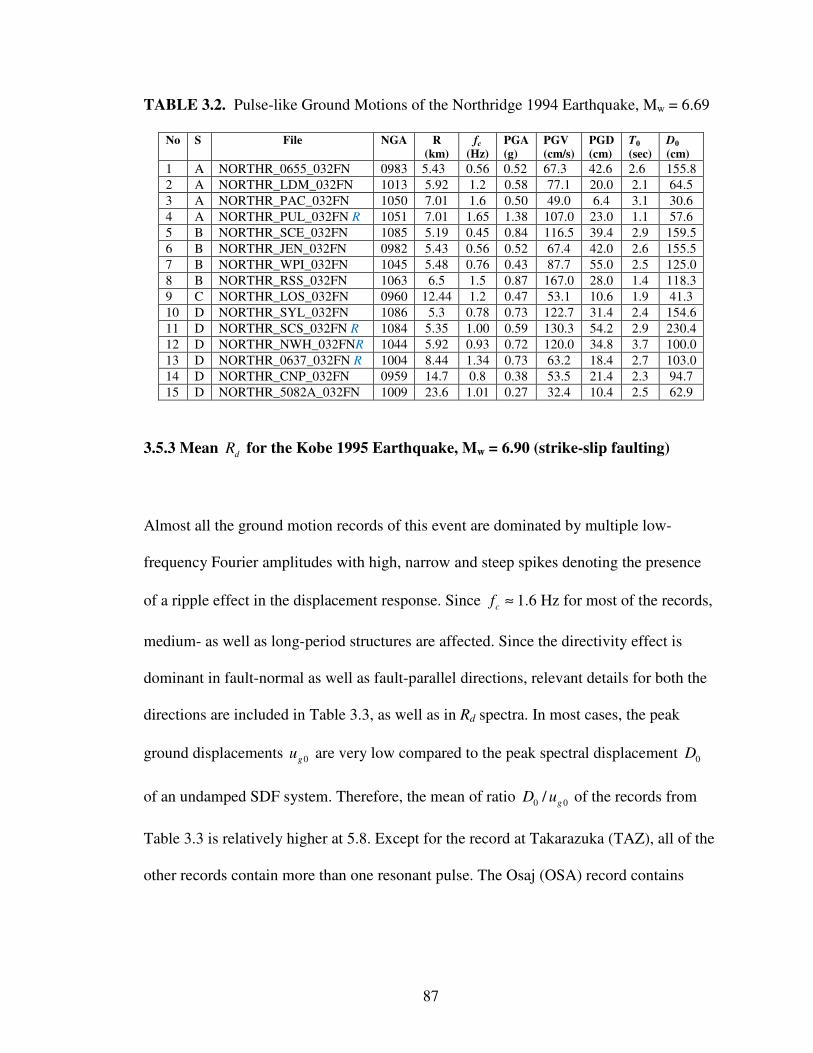
87
TABLE 3.2. Pulse-like Ground Motions of the Northridge 1994 Earthquake, Mw = 6.69
No S File NGA R
(km)
fc
(Hz)
PGA
(g)
PGV
(cm/s)
PGD
(cm)
T0
(sec)
D0
(cm)
1 A NORTHR_0655_032FN 0983 5.43 0.56 0.52 67.3 42.6 2.6 155.8
2 A NORTHR_LDM_032FN 1013 5.92 1.2 0.58 77.1 20.0 2.1 64.5
3 A NORTHR_PAC_032FN 1050 7.01 1.6 0.50 49.0 6.4 3.1 30.6
4 A NORTHR_PUL_032FN R 1051 7.01 1.65 1.38 107.0 23.0 1.1 57.6
5 B NORTHR_SCE_032FN 1085 5.19 0.45 0.84 116.5 39.4 2.9 159.5
6 B NORTHR_JEN_032FN 0982 5.43 0.56 0.52 67.4 42.0 2.6 155.5
7 B NORTHR_WPI_032FN 1045 5.48 0.76 0.43 87.7 55.0 2.5 125.0
8 B NORTHR_RSS_032FN 1063 6.5 1.5 0.87 167.0 28.0 1.4 118.3
9 C NORTHR_LOS_032FN 0960 12.44 1.2 0.47 53.1 10.6 1.9 41.3
10 D NORTHR_SYL_032FN 1086 5.3 0.78 0.73 122.7 31.4 2.4 154.6
11 D NORTHR_SCS_032FN R 1084 5.35 1.00 0.59 130.3 54.2 2.9 230.4
12 D NORTHR_NWH_032FNR 1044 5.92 0.93 0.72 120.0 34.8 3.7 100.0
13 D NORTHR_0637_032FN R 1004 8.44 1.34 0.73 63.2 18.4 2.7 103.0
14 D NORTHR_CNP_032FN 0959 14.7 0.8 0.38 53.5 21.4 2.3 94.7
15 D NORTHR_5082A_032FN 1009 23.6 1.01 0.27 32.4 10.4 2.5 62.9
3.5.3 Mean d
R for the Kobe 1995 Earthquake, Mw = 6.90 (strike-slip faulting)
Almost all the ground motion records of this event are dominated by multiple low-
frequency Fourier amplitudes with high, narrow and steep spikes denoting the presence
of a ripple effect in the displacement response. Since c
f ≈ 1.6 Hz for most of the records,
medium- as well as long-period structures are affected. Since the directivity effect is
dominant in fault-normal as well as fault-parallel directions, relevant details for both the
directions are included in Table 3.3, as well as in Rd spectra. In most cases, the peak
ground displacements 0gu are very low compared to the peak spectral displacement 0D
of an undamped SDF system. Therefore, the mean of ratio 0 0/g
D u of the records from
Table 3.3 is relatively higher at 5.8. Except for the record at Takarazuka (TAZ), all of the
other records contain more than one resonant pulse. The Osaj (OSA) record contains

88
resonant pulses at four frequencies, affecting displacement response spectra (DRS) at
corresponding n
T = 1.9, 3.2, 3.6 and 4.4 seconds.
It has been observed that low-velocity soft and near-surface sediments are effective in
amplifying and elongating long-period ground motions [Hatayama et al., 2007; Miyake
and Koketsu 2007]. At stations Takarazuka (TAZ) and Shin-Osaka (SHI), the spectral
displacements due to fault-parallel components are higher than those due to fault-normal
ones, denoting that the site effects may be more dominant than the directivity effect.
In Fig. 3.12.a and 3.12.b, the mean and the mean+one stdv d
R spectra for the Kobe 1995
earthquake are plotted for three damping ratios, ζ =0, 0.02 and 0.05. In these figures, it
can be seen that the maximum mean d
R values are 9.41, 5.58 and 4.04 for ζ = 0, 0.02
and 0.05, respectively, and the maximum mean+one stdv d
R values for the same event
are 14.20, 6.92 and 4.80 for ζ = 0, 0.02 and 0.05, respectively. This event has the highest
Rd values of all the events considered in this study (Fig. 3.19).
In a similar manner, the mean displacement response factor may be evaluated for (a) the
2003 Tokachi-oki, Japan, earthquake, (b) the 2004 South-East off Kii peninsula
earthquake, (c) the 2004 Niigata-ken Chuetsu, Japan earthquake, and (d) the 2007
Niigata-ken Chuetsu-oki, Japan earthquake. This would probably establish a range of
mean ± one stdv factors for Japan. This Rd value may be useful in the design of dampers
for the structures in Japan.

89
0
2
4
6
8
10
0 0.5 1 1.5 2
0
2
4
6
8
10
12
14
0 0.5 1 1.5 2
Figure 3.12 Modified displacement response factor for the Kobe 1995 earthquake
Rd spectra for (a) the mean values (b) the mean+one stdv values
TABLE 3.3. Pulse-like Ground Motions of the Kobe1995 Earthquake, Mw = 6.9
No S File NGA R
(km)
fc
(Hz)
PGA
(g)
PGV
(cm/s)
PGD
(cm)
T0
(sec)
D0
(cm)
1 B KOBE_KJM_140FN R 1106 0.96 1.56 0.85 95.8 24.6 1.02 101
1a KOBE_KJM_050FP R - - 1.67 0.55 53.4 10.3 1.3 55.8
2 D KOBE_TAZ_140FN 1119 0.27 1.64 0.65 72.5 20.8 2.0 74.5
2a KOBE_TAZ_050FP - - 0.85 0.70 83.0 26.5 1.6 87.6
3 E KOBE_TAK_140FN R 1120 1.47 0.98 0.68 169.2 45.0 2.1 273.6
3a KOBE_TAK_050FP R - - 1.00 0.61 169.6 22.9 3.1 130.0
4 E KOBE_SHI_140FN R 1116 19.15 1.66 0.19 30.0 8.8 2.7 38.6
4a KOBE_SHI_050FP R - - 1.64 0.27 41.8 7.4 1.2 41.4
5 E KOBE_ OSA_140FN R 1113 21.35 0.68 0.07 20.0 9.8 4.4 86.1
5a KOBE_ OSA_050FP R - - 0.64 0.08 17.1 7.9 3.4 78.8
The PGA, PGV and maximum spectral displacement D0’s for the OSA_140FN station
are 0.073g, 20 cm/s and 86.1 cm, respectively. Although KOBE_TAZ_050FP
ζ=0.0
ζ=0.02
ζ=0.05
ζ=0.0
ζ=0.02
ζ=0.05
Tn/Tp
Tn/Tp
Rd
Rd
(a)
(b)

90
(Takarazuka) has a high PGA (0.70g) and PGV (83 cm/sec), its maximum spectral
displacement D0 = 87.6 cm/s ≈ D0 = 86.1 cm/s of Osaj. Similarly, KOBE_SHI_050FP
(Shin-Osaka) has a high PGA (0.27g) and PGV (42 cm/sec), its maximum spectral
displacement D0 = 41.4 cm/s << D0 = 86.1 cm/s of Osaj. This shows that the maximum
spectral displacement, D0, may not be directly related to the PGA or PGV. Similar
observations may be made from the records of other events.
3.5.4 Mean d
R for the Loma Prieta 1989 Earthquake, Mw = 6.93 (reverse/oblique
faulting)
The Loma Prieta 1989 event in North America may be considered the most destructive
one among other events of N. America. Seven out of the thirteen pulse-like records
contain resonant pulses, therefore the mean and mean+one stdv are comparatively higher.
The velocity Fourier amplitudes in 1.67 c
LUF f f Hz≤ ≤ < are dominated by multiple,
steep and high spikes, characterizing a ripple effect. Multiple high-spectral displacements
are observed at multiple periods of vibrations in the displacement response spectra.
Therefore, both medium- as well as long-period structures are affected. This can also be
observed in Table 3.4.
From the seventh column of Table 3.4, it can be observed that the PGA varies from 0.94g
to 0.12g, as the distance from the fault-rupture R varies from 3.88 km to 77.4 km;
however, the displacement response factor d
R is independent of this change. The mean of
the maximum values of d
R for station # 1 to 5 is around 6.1 for ζ =0; however, at each

91
station from # 6 to #12, d
R is more than 10.0 for the same damping ratio. Thus, d
R may
not be dependent upon the PGA. This important observation may be borne in mind when
designing structures in near-fault areas or on distant sedimentary basins.
In Fig. 3.13.a and 3.13.b, the mean and the mean+one stdv d
R spectra for the Loma
Prieta 1989 earthquake are plotted for three damping ratios, ζ =0, 0.02 and 0.05. From
these figures, it can be seen that the maximum mean d
R values are 7.05, 4.97 and 3.72
for ζ = 0, 0.02 and 0.05, respectively; and the maximum mean+one stdv d
R values for
the same event are 10.13, 6.51 and 4.71 for ζ = 0, 0.02 and 0.05, respectively.

92
Rd
0
2
4
6
0 0.5 1 1.5 2
0
2
4
6
8
10
0 0.5 1 1.5 2
Figure 3.13 Modified displacement response factor for the Loma Prieta 1989
Earthquake: Rd Spectra for (a) the mean values (b) the mean+one stdv values
Tn/Tp
Tn/Tp
ζ=0.0
ζ=0.02
ζ=0.05
ζ=0.0
ζ=0.02
ζ=0.05
(a)
(b)
Rd
Rd

93
TABLE 3.4. Pulse-like Ground Motions of the Loma Prieta 1989 Earthquake, Mw = 6.93
No S File NGA R
(km)
fc
(Hz)
PGA
(g)
PGV (cm/s)
PGD
(cm)
T0
(sec)
D0
(cm) Rd
1 A LOMAP_LGP_038FN 0779 3.88 0.84 0.94 96.5 62.5 5.6 168. 5.4
2 A LOMAP_LEX_038FN 3548 5.02 1.28 0.52 102. 34.0 1.1 76.7 5.8
3 A LOMAP_G01_038FN 0765 6.93 0.92 0.43 40.0 7.2 3.0 29.0 6.6
4 B LOMAP_GIL_038FN 0763 6.93 0.92 0.29 31.0 6.5 3.0 25.3 6.3
5 D LOMAP_STG_038FN 0802 8.5 1.15 0.36 56.0 29.4 6.5 91.5 6.4
6 D LOMAP_WVC_038FN,R 0803 9.31 1.00 0.40 71.0 21.0 2.8 101. 13.4
7 D LOMAP_GOF_038FN, R 0764 10.97 1.13 0.25 22.0 4.5 1.0 27.5 15.2
8 D LOMAP_G02_038FN, R 0766 11.07 0.85 0.41 46.0 13.0 1.5 63.8 10.6
9 D LOMAP_G03_038FN, R 0767 12.82 0.95 0.53 49.0 11.0 1.5 44.5 10.3
10 D LOMAP_G04_038FN, R 0768 14.34 0.85 0.35 36.0 11.5 1.4 52.0 12.
11 D LOMAP_CH1_038FN, R 0783 74.26 0.80 0.33 49.0 12.8 1.5 50.8 10.
12 E LOMAP_NAS_038FN, R 0738 71.00 0.54 0.22 32.0 10.3 2.4 54.0 10.3
13 E LOMAP_TRI_038FN 0808 77.42 1.25 0.12 27.2 9.2 2.5 40.5 5.5
Rd values are calculated for the record at each station, and entered in the last column. The
last three examples, numbered 11, 12 and 13 in Table 3.4 for the Oakland - Outer Harbor
Wharf, the Alameda Naval Air Station Hanger stations and Treasure Island, may be noted
as examples of the path-effect, since these stations are located at distances of 74.26 km
(46.14 miles), 71 km (44.12 miles) and 77.42 km (48.4 miles) from the fault-rupture,
respectively. Far-source ground motions consist of surface waves which may have a
longer duration than those of near-fault motions. They can be very damaging in some
circumstances. An example is the 1985 Michoacan earthquake, which occurred in the
sedimentary basins of Mexico City, which was 350 km away from the epicenter.
3.5.5 Mean d
R for the Kocaeli 1999 Earthquake, Mw = 7.51 with the Duzce-Bolu
1999, Mw = 7.14 and the Erzican-Erz 1992, Mw = 6.69 (strike-slip faulting)
Although pulse-effect is not apparent [Park et al., 2004] in the velocity time history, the
DUZCE_BOL_175FN 1999 earthquake record has resonant pulses at n
T = 1.2, 1.9, 2.8
94
and 4.5 seconds, which is evident from its DRS (not shown), as well as in its velocity
Fourier spectra (not shown). This record at Bolu has high d
R = 13.8, 7.6 and 5.0, for ζ =
0, 0.02 and 0.05, respectively. The Duzce November 1999 earthquake caused a surface
rupture across the Bolu viaduct, which resulted in excessive superstructure movement
and widespread failure of the seismic isolation system. The displacement of the
superstructure relative to the piers exceeded the capacity of the bearings at an early stage
of the earthquake, causing damage to the bearings as well as to the energy dissipation
units [Park et al., 2004].
At Yarimca (YPT), the spectral displacements in fault-parallel directions are more
dominant. The c
f for the majority of records of Kocaeli 1999 event are less than 0.4 Hz.
Large spectral displacements are observed at larger periods of vibration. The mean period
of vibration with maximum spectral displacements is around 9 seconds for the Kocaeli
August 1999 event.
In Fig. 3.14.a and 3.14.b, the mean and the mean+one stdv d
R spectra for pulse-like
ground motions near the North Anatolian Fault, Turkey, are plotted for three damping
ratios, ζ =0, 0.02 and 0.05. From these figures, it can be seen that the maximum mean
dR values are 6.03, 4.43 and 3.50 for ζ = 0, 0.02 and 0.05, respectively; and the
maximum mean+one stdv d
R values for the same event are 9.10, 5.80 and 4.23 for ζ = 0,
0.02 and 0.05, respectively.

95
0
1
2
3
4
5
6
0 0.5 1 1.5 2
0
1
2
3
4
5
6
7
8
9
0 0.5 1 1.5 2
Figure 3.14 Modified displacement response factor for the North Anatolian Fault,
Turkey: Rd spectra for (a) the mean values (b) the mean+one stdv values
TABLE 3.5. Pulse-like Ground Motions near the North Anatolian Fault, Turkey
No S File NGA R
(km)
fc
(Hz)
PGA
(g)
PGV
(cm/s)
PGD
(cm)
T0
(sec)
D0
(cm)
1 A KOCAELI_GBZ_184FN 1161 10.92 0.39 0.24 51.9 44.0 9.5 155.4
2 B KOCAELI_SKR_090 1171 3.12 0.28 0.38 79.5 72.3 14.0 212
3 B KOCAELI_ARC_184FN 1148 13.49 0.40 0.17 20.3 16.0 8.9 60.8
4 D KOCAELI_YPT_180FN 1176 4.43 0.40 0.28 48.2 44.0 5.1 179.2
4a D KOCAELI_YPT_090FP - - 0.37 0.31 72.9 56.2 3.6 220.0
5 D KOCAELI_DZC_163FN 1158 15.37 0.37 0.28 52.2 38.0 6.8 144.0
5a D KOCAELI_DZC_073FP - - 0.74 0.38 53.0 26.5 6.0 130.0
6 D ERZIKAN_ERZ_032FN 0821 4.38 0.67 0.49 95.4 32.9 3.0 133.8
6a D ERZIKAN_ERZ_122FP - - 0.82 0.42 45.3 16.5 2.7 90.5
7 D DUZCE_BOL_175FN R 1602 12.04 0.59 0.68 57.5 23.0 1.9 85.0
ζ=0.0
ζ=0.02
ζ=0.05
ζ=0.0
ζ=0.02
ζ=0.05
Tn/Tp
Tn/Tp
Rd
Rd
(b)
(a)

96
3.5.6 Mean d
R for the Chi-Chi 1999 Earthquake, Mw=7.62 (reverse/oblique faulting)
This event is characterized by extreme ground displacements. Designing for high ground
displacements (fling) in most cases would probably control for such types of event. d
R
factor for this event is relatively less than most other events.
As seen in the 5th
column of Table 3.6, all the eight records are very close (< 5.3 km) to
the fault-rupture. Stations TCU052 and TCU068 are at the Hanging wall sides. The
spectral displacements at these two stations more or less monotonically increase as the
period of vibration n
T increases (Fig. 3.2.a for TCU052). The remaining six stations are
situated at the foot-wall of the fault-rupture. As seen in Table 3.6, extreme PGVs, PGDs,
as well as spectral displacements, are observed.
The peak ground displacements (PGDs) are very high, the average of the eight stations
being 150 cm. The mean ratio of 0 0/g
D u of the records from Table 3.6 is comparatively
lower at 3.5. Recall from Sec. 3.5.3 that this value for the Kobe 1995 event is 5.8.
In Fig. 3.15.a and 3.15.b, the mean and the mean+one stdv d
R spectra for the Chi-Chi
1999 earthquake are plotted for three damping ratios, ζ =0, 0.02 and 0.05. From these
figures, it can be seen that the maximum mean d
R values are 5.26, 3.78 and 3.02 for ζ =
0, 0.02 and 0.05, respectively; and the maximum mean+one stdv d
R values for the same
event are 7.40, 4.92 and 3.69 for ζ = 0, 0.02 and 0.05, respectively.

97
Rd
0
1
2
3
4
5
0 0.5 1 1.5 2
0
1
2
3
4
5
6
7
0 0.5 1 1.5 2
Figure 3.15 Modified displacement response factor for the Chi-Chi 1999 earthquake:
Rd spectra for (a) the mean values (b) the mean+one stdv values
TABLE 3.6. Pulse-like Ground Motions of the Chi-Chi 1999 Earthquake, Mw = 7.62
No S File NGA R
(km)
fc
(Hz)
PGA
(g)
PGV
(cm/s)
PGD
(cm)
T0
(sec)
D0
(cm)
1 A CHICHI_TCU068_N320E 1505 0.32 0.3 0.57 290.0 475.0 12.4 1209.
2 A CHICHI_TCU052_N322E 1492 0.66 0.28 0.50 167.0 306.0 17.3 814.0
3 A CHICHI_TCU102_N232E 1529 1.51 0.47 0.24 110.0 91.3 7.6 338.0
4 D CHICHI_TCU065_N123E 1503 0.59 0.28 0.82 130.0 93.0 5.3 495.0
5 D CHICHI_TCU075_N094E 1510 0.91 0.36 0.33 88.6 86.0 3.9 247.0
6 D CHICHI_TCU129_N136E 1549 1.84 0.29 0.83 57.0 52.0 5.8 187.0
7 D CHICHI_TCU076_N128E 1511 2.76 0.49 0.35 88.0 41.0 7.9 151
8 D CHICHI_TCU054_N142E 1494 5.30 0.26 0.18 59.1 63.0 9.2 232
ζ=0.0
ζ=0.02
ζ=0.05
ζ=0.0
ζ=0.02
ζ=0.05
Tn/Tp
Tn/Tp
(b)
(a)
Rd
Rd
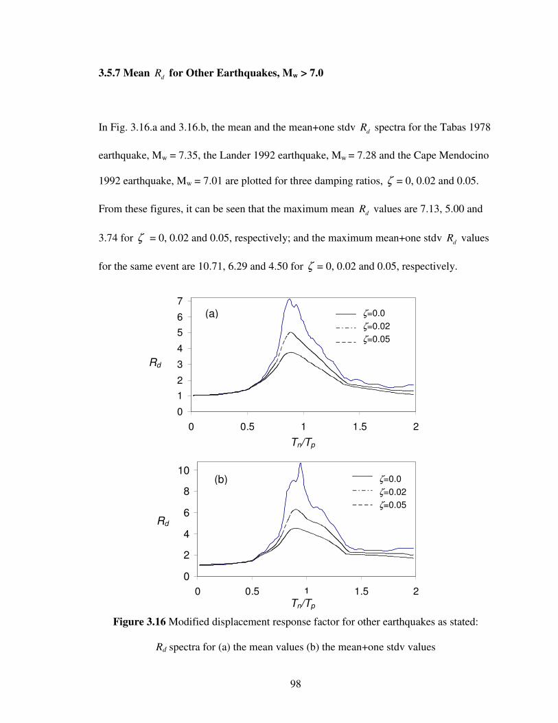
98
3.5.7 Mean d
R for Other Earthquakes, Mw > 7.0
In Fig. 3.16.a and 3.16.b, the mean and the mean+one stdv d
R spectra for the Tabas 1978
earthquake, Mw = 7.35, the Lander 1992 earthquake, Mw = 7.28 and the Cape Mendocino
1992 earthquake, Mw = 7.01 are plotted for three damping ratios, ζ = 0, 0.02 and 0.05.
From these figures, it can be seen that the maximum mean d
R values are 7.13, 5.00 and
3.74 for ζ = 0, 0.02 and 0.05, respectively; and the maximum mean+one stdv d
R values
for the same event are 10.71, 6.29 and 4.50 for ζ = 0, 0.02 and 0.05, respectively.
0
1
2
3
4
5
6
7
0 0.5 1 1.5 2
0
2
4
6
8
10
0 0.5 1 1.5 2
Figure 3.16 Modified displacement response factor for other earthquakes as stated:
Rd spectra for (a) the mean values (b) the mean+one stdv values
Rd
Rd
Tn/Tp
Tn/Tp
ζ=0.0
ζ=0.02
ζ=0.05
ζ=0.0
ζ=0.02
ζ=0.05
(a)
(b)

99
TABLE 3.7. Other Pulse-like Ground Motions, Mw > 7
No S File NGA R
(km)
fc
(Hz)
PGA
(g)
PGV
(cm/s)
PGD
(cm)
T0
(sec)
D0
(cm)
1 A TABAS_TAB_TR 143 2.05 0.27 0.85 121.1 95 4.7 419
2 A LANDERS_LCN_239FN 879 2.19 0.40 0.69 136.1 236 11.2 222
3 D LANDERS_YER_240FN 900 23.6 0.86 0.23 56.2 48 7.8 141
4 D LANDERS_BRS_240FN 838 34.9 0.40 0.14 30.9 27 8.4 80
5 B CAPEMEND_PET260FN 828 8.18 1.28 0.62 81.9 25 2.2 67
3.5.8 Summary
TABLE 3.8. Summary of d
R for different events
mean values mean+one stdv values
No EVENT ζ=0.0 ζ=0.02 ζ=0.05 ζ=0.0 ζ=0.02 ζζζζ=0.05
1 Imperial Valley 1979, Mw = 6.53 4.85 3.66 3.05 5.91 4.29 3.44
2 Northridge 1994, Mw = 6.69 6.18 4.39 3.41 8.37 5.55 4.17
3 Kobe 1995, Mw = 6.90 9.41 5.58 4.04 14.20 6.92 4.80
4 Loma Prieta 1989, Mw = 6.93 6.8 4.7 3.6 10.0 6.2 4.5
5 Kocaeli 1999, Mw = 7.51 6.03 4.43 3.50 9.10 5.80 4.23
6 Chi-Chi 1999, Mw = 7.62 5.26 3.78 3.02 7.40 4.92 3.69
7 Other earthquakes, Mw > 7 7.14 5.00 3.74 10.71 6.29 4.50
If we assume ζ = 0.02 for most long-period structures, an appropriate and recommended
Rd value for the design of such structures is between five to seven (the mean+one stdv
values), signifying that these structures would demand very high strength. For ζ = 0.05,
the (m+σ) values of Rd vary from 3.44 to 4.8. The summary of values Rd in Table 3.8
shows that when considering different events all over the world, the value of the
displacement response factor Rd may not always be directly proportional to the moment
magnitude of the event. These may depend more upon directivity, and the site, as well as
upon the path effects.

100
3.6 OBSERVATIONS
3.6.1 Comparison of seismic Rd with that due to simple harmonic excitation
The equation of motion for a SDF damped system subjected to harmonic force ( )p t is
given by [Clough and Penzien 1992; Chopra 2007; Humar 1992]
0 sinmu cu ku p tω+ + =&& & (3.9)
The displacement response factor of the steady-state deformation of the system due to
harmonic force is given by
( ) [ ]
0
2 220
1
1 ( / ) 2 ( / )d
stn n
uR
u ω ω ζ ω ω= =
− +
(3.10)
In Eq. (3.10), the Rd = 10 for ζ = 0.05 and (ω/ωn) = 1. In Table 3.8, the (m+σ) values of
Rd vary from 3.44 to 4.8 for ζ = 0.05 for different earthquake events. If we substitute the
value of Rd = 3.44 in Eq. (3.10), we get an equivalent (ω/ωn) = 0.85 and 1.125 for the
Imperial Valley-6 1979 event. Similarly, if we substitute Rd = 4.8 in Eq. (3.10), we get an
equivalent (ω/ωn) = 0.9 and 1.085 for the Kobe 1995 event. Therefore, for pulse-like
complex seismic ground motions, we may equivalently adopt 0.85 ≤ (ω/ωn) ≤ 0.9 or
1.125 ≥ (ω/ωn) ≥ 1.085.
Fig. 3.17. shows the (m+σ) Rd values of the Imperial Valley-6 1979 event plotted against
Tn/Tp for ζ = 0.05 in blue. The (m+ σ) Rd values of the Kobe 1995 event are also plotted
against Tn/Tp for ζ = 0.05 in red. Rd values for harmonic excitation as given by Eq. (3.10)
for ζ = 0.05 is also plotted in black for comparison. Observe that the concept of

101
equivalent forcing frequency (ω/ωn) ratio holds true for the events with the lowest (the
Imperial Valley-6 1979) and the highest (the Kobe 1995) Rd.
To compare Rd spectra of each event with that from continuous harmonic excitation, it is
proposed to modify Eq. (3.10) as follows,
( ) [ ]
0
2 220
1
1 ( / ) 2 ( / )d
stn n
uR
ukω αω ζ ω αω
= = − +
(3.11)
where, n
n p
T
T
αω
ω=
(αTn) is the effective natural period of vibration of the system. α is a period shift factor
and k is a damping modification factor. The Imperial Valley-6 1979 event has the lowest
Rd = 3.44. For α = 0.9 and k = 2.95 (obtained by iteration), the modified (m+σ) Rd spectra
obtained from Eq. (3.11) is plotted in Fig. 3.18 in blue line. It is comparable for Rd and
phase values with the (m+σ) Rd spectra of the same event (from Fig. 3.10.b) plotted in
blue dashed line.
Modified (m+σ) Rd spectra (red line) obtained from Eq. (3.11) for α = 0.77 and k = 2.1
(obtained by iteration) for the Kobe 1995 event is superimposed on the original Kobe
1995 (m+σ) Rd spectra (from Fig. 3.12.b) as shown in red dashed line. From Fig. 3.18, it
is observed that both have a comparable Rd values, as well as periods. Thus, for 0.77
(Kobe) ≤ α ≤ 0.9 (Imperial V) and for 2.1 (Kobe) ≤ k ≤ 2.95 (Imperial V), we can
equivalently represent Rd for all the six major events under consideration.

102
Figure 3.17. Concept of equivalent harmonic forcing frequency (ω/ωn) ratio illustrated
for Imperial Valley-6 1979 and Kobe 1995 events, comparing with harmonic excitation.
Figure 3.18. Concept of combined factors k & α illustrated for Imperial Valley-6 1979
and Kobe 1995 events, comparing with equivalent harmonic excitation, Eq. (3.11)
Imperial V 1979
Kobe 1995
Harmonic
Tn/Tp
Rd
Eqv. Harmonic
Imperial V 1979
Eqv. Harmonic
Kobe 1995
Tn/Tp
Rd
(ω/ωn) = 0.9
(ω/ωn) = 0.85

103
Figure 3.19. Displacement Response Factor, Rd for each major earthquake events
compared with that due to simple continuous harmonic excitation, ζ = 0.05
Thus, for pulse-like seismic ground motions, the concept of an equivalent harmonic
forcing frequency ratio (ω/ωn) or a ‘damping modification factor’ may be introduced.
This concept helps us to compare the values of dynamic magnification among different
earthquake events, as well as those due to simple harmonic excitation. Since damping
Dis
pla
cem
ent
Response
Facto
r, R
d
Tn/Tp
Harmonic, Rd = 10
Imperial V, Rd =3.44
Chi-Chi, Rd = 3.69
NorthR, Rd = 4.17
Kocaeli, Rd = 4.23
LomaP, Rd = 4.50
Kobe 1995, Rd = 4.80

104
controls the response characteristics of such structures, these Rd values can help us to
design dampers that can sustain pulse-like excitations.
The concept of equivalent viscous damping is not new, it was first proposed by Jacobsen
in 1930 to obtain approximate solutions for the steady forced vibration of damped SDF
systems with linear force-displacement relationships but with damping forces
proportional to the nth power of the velocity of motion when subjected to sinusoidal
forces. In 1960, he extended the concept of equivalent viscous damping to yielding SDF
systems. Since then, many methods have been proposed in the literature [Sec. 3.3.1 of
FEMA 440, 2005].
3.6.2 RESPONSE AND DAMPING
In the preceding section, it was seen that 0.85 ≤ (ω/ωn) ≤ 0.9, i.e., the forcing frequency is
close to the natural frequency of the system. Therefore, it is known [Clough and Penzien
1992; Chopra 2007; Humar 1992] that Rd is very sensitive to damping. When (ω/ωn) ≈ 1,
and k is such that 2.1 ≤ k ≤ 2.95, then Eq. (3.10) becomes
0 00
( )
2. . . .
st
n
u pu
k k cζ ω= = (3.12)
where c is the damping coefficient. Thus, damping controls the response of systems
subjected to such pulse-like near-fault ground motions. The Rd values calculated from
different events can assist us with the design of dampers that can sustain pulse-like
excitations.

105
3.7 SUMMARY AND CONCLUSIONS
The modified displacement response factor is defined as the ratio of the maximum
amplitude 0u D≡ of the dynamic deformation to the maximum static deformation 0( )st
u ,
when a linearly elastic SDF system is subjected to a pulse excitation ( )p
p t in the
dynamic analysis, and to a static load 0 0p ma= − (where 0p is the amplitude or
maximum value of the excitation having excitation frequency cω ω≤ ) in the static
analysis. This is a simple but very useful tool that helps in the determination of dynamic
amplification. The statistical study for the mean and the (mean+one stdv) values of d
R
for different earthquake events were evaluated for comparison with each other.
Rd values obtained for each earthquake events were compared with that caused due to
simple harmonic excitation. The concepts of equivalent forcing frequency ratio (ω/ωn), a
period shift factor α and damping modification factor k were introduced to facilitate the
comparison with simple harmonic excitation. The Rd values calculated from different
events can assist us in the design of dampers, which would be able to sustain pulse-like
excitations.
Based on the results of this study, the following conclusions can be drawn:
1. A simple sine-pulse (single-period pulse) does not always give a good
representation of ground motions in response identification. The use of a sine-
pulse should be limited to those response characteristics in which the spectral
displacement more or less increases monotonically with a natural period n
T from

106
the cut-off frequency to the frequency that corresponds to the peak of the spike
nearest the lowest usable frequency.
2. In most cases (e.g., Figs. 3.2.a, 3.4.a, 3.5.b & 3.7.a), it has been observed that
displacement response cannot be simplistically obtained from a single sine pulse.
A full sinusoidal pulse gives the lower bound value of Rd for any pulse-like
record; whereas a continuous harmonic excitation gives the upper bound value of
Rd. It is the succession of sinusoidal pulses for a finite duration that give rise to
such high value of Rd.
3. In the present study, not a single velocity-pulse extracted from the 72 ground
motions by the proposed signal processing technique was found to have a half-
cycle velocity pulse. Around ten records have a predominant single period
velocity pulse, but most other pulses are multiple-period pulses. That is one of the
reasons why Rd exceeds 3.14.
4. A number of NFGMs exhibit a ripple effect in which maximum spectral
displacements are observed at different natural periods. This is the result of the
presence of multiple predominant frequency pulses in these earthquake records.
5. Resonance pulses are special cases of multiple frequency pulses when the
dynamic displacements are very high compared to their static counterparts. These
pulses are identified as high, steep and narrow amplitude spikes in the velocity
Fourier spectrum. Their magnitudes can be quantified by the use ofd
R .
6. Velocity Fourier spectrum is an important tool for design engineers to use, to
characterize the displacement response of SDF systems.
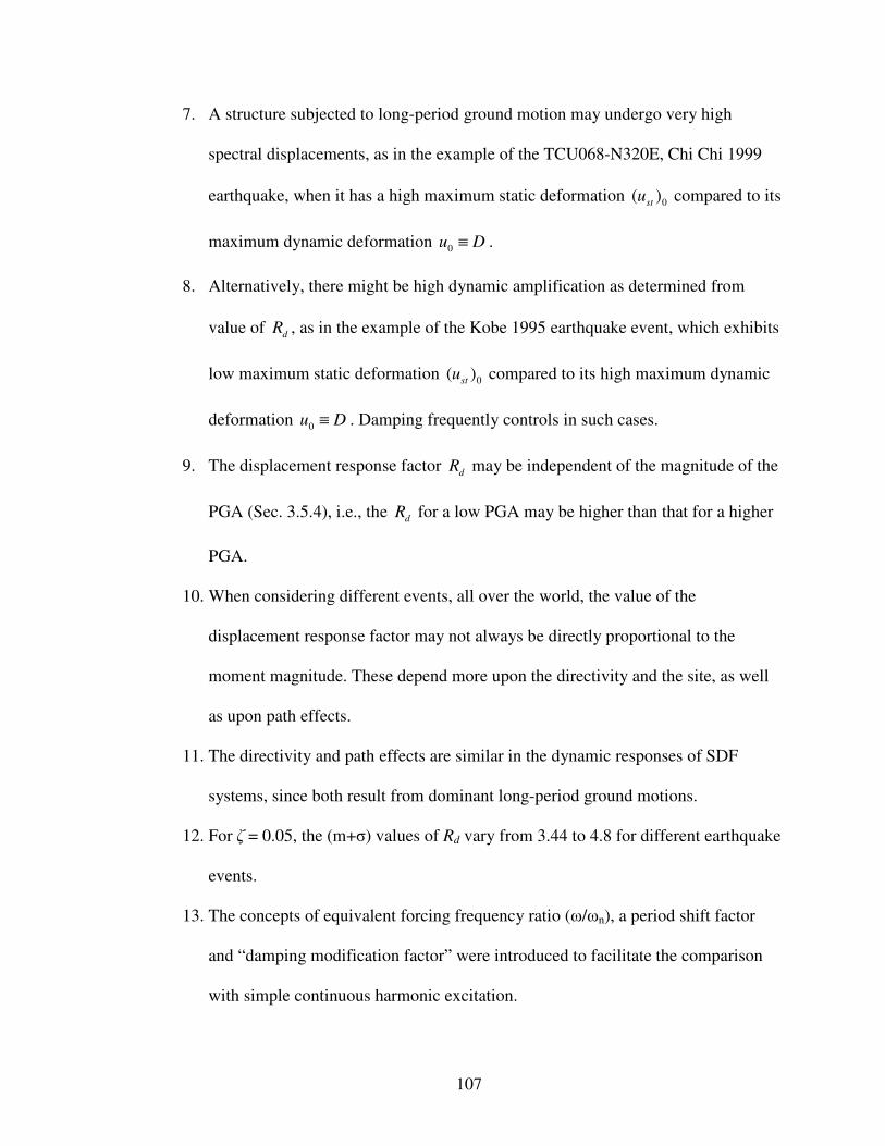
107
7. A structure subjected to long-period ground motion may undergo very high
spectral displacements, as in the example of the TCU068-N320E, Chi Chi 1999
earthquake, when it has a high maximum static deformation 0( )st
u compared to its
maximum dynamic deformation 0u D≡ .
8. Alternatively, there might be high dynamic amplification as determined from
value of d
R , as in the example of the Kobe 1995 earthquake event, which exhibits
low maximum static deformation 0( )st
u compared to its high maximum dynamic
deformation 0u D≡ . Damping frequently controls in such cases.
9. The displacement response factor d
R may be independent of the magnitude of the
PGA (Sec. 3.5.4), i.e., the d
R for a low PGA may be higher than that for a higher
PGA.
10. When considering different events, all over the world, the value of the
displacement response factor may not always be directly proportional to the
moment magnitude. These depend more upon the directivity and the site, as well
as upon path effects.
11. The directivity and path effects are similar in the dynamic responses of SDF
systems, since both result from dominant long-period ground motions.
12. For ζ = 0.05, the (m+σ) values of Rd vary from 3.44 to 4.8 for different earthquake
events.
13. The concepts of equivalent forcing frequency ratio (ω/ωn), a period shift factor
and “damping modification factor” were introduced to facilitate the comparison
with simple continuous harmonic excitation.

108
14. The Rd values calculated from different events may assist us in designing
dampers, which can sustain pulse-like excitations.
During the evaluation of responses, we have observed very important properties of
velocity Fourier spectrum. We have seen that the Fourier spectrum effectively helps us to
determine spectral displacements. This observation will be used in the next chapter to
propose an analogous displacement response spectrum.

109
CHAPTER 4
ANALOGOUS DISPLACEMENT RESPONSE SPECTRA
4.1 INTRODUCTION
In chapter 2, we detected directivity effects in ground motions by signal processing using
Fourier analysis. A structural engineer is generally more interested in the natural period
of vibration of a system and the period of excitation. Therefore, Fourier analysis is
applied when the frequency contents of the excitation are of greater importance. In the
previous two chapters, we have also seen that the velocity Fourier spectrum is the key to
understanding spectral displacements, as well as dynamic magnification.
The evaluation and plotting of the displacement response spectra (DRS) for a number of
pulse-like ground motions have shown that they bear a strong mirror image resemblance
to ground velocity Fourier amplitudes. The peak spectral displacements in the DRS occur
at natural periods of vibration Tn, which correspond to the frequencies at which the
magnitudes of the Fourier amplitudes are at their peaks. The values of frequencies on the
abscissa of the VFA closely correspond to the reciprocal values of system periods Tn on
the abscissa of the DR spectrum, while the values on the y-axis (the velocity Fourier
amplitudes in g-s) of the VFA nearly correspond to those on the y-axis (spectral
displacements in cm) of the DR spectrum.
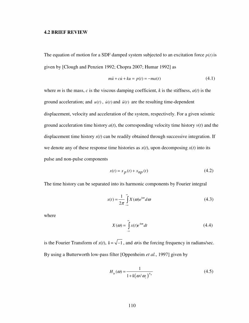
110
4.2 BRIEF REVIEW
The equation of motion for a SDF damped system subjected to an excitation force ( )p t is
given by [Clough and Penzien 1992; Chopra 2007; Humar 1992] as
( ) ( )mu cu ku p t ma t+ + = = −&& & (4.1)
where m is the mass, c is the viscous damping coefficient, k is the stiffness, a(t) is the
ground acceleration; and ( )u t , ( )u t& and ( )u t&& are the resulting time-dependent
displacement, velocity and acceleration of the system, respectively. For a given seismic
ground acceleration time history a(t), the corresponding velocity time history v(t) and the
displacement time history s(t) can be readily obtained through successive integration. If
we denote any of these response time histories as x(t), upon decomposing x(t) into its
pulse and non-pulse components
)()()( tnpxtpxtx += (4.2)
The time history can be separated into its harmonic components by Fourier integral
1
( ) ( )2
tx t X e d
ωω ωπ
∞
−∞
= ∫i (4.3)
where
( ) ( )t
X x t e dtωω
∞
−∞
= ∫-i (4.4)
is the Fourier Transform of x(t), 1= −i , and ω is the forcing frequency in radians/sec.
By using a Butterworth low-pass filter [Oppenheim et al., 1997] given by
( )
1( )
1 / Blp N
c
H ωω ω
=+ i
(4.5)

111
where ωc is the cut-off frequency in radians/sec., and NB is the order of the Butterworth
filter. By using a suitable cut-off frequency fc=ωc/2π, the pulse component can be
evaluated using the equation
1( ) ( ) ( )
2
t
p lpx t H X e d
ωω ω ωπ
∞
−∞
= ∫i (4.6)
If we replace ( ) ( )lp
H Xω ω by ( )p
X ω , we can rewrite Eq. (4.6) as
1
( ) ( )2
t
p px t X e d
ωω ωπ
∞
−∞
= ∫i (4.7)
The pulse xp(t) obtained from Eq. (4.7) can be used in a time-domain analysis to compute
spectral displacements. In the following study, Eq. (4.7) is used to compute acceleration
and velocity pulse histories. It should be noted that in this chapter, the pulse component
of a time history is considered to be synonymous with the dominant low-frequency
contents of that time history.
4.3 SPECTRAL DISPLACEMENTS AND FOURIER AMPLITUDES
In this section, a method is proposed for expressing spectral displacements for an
undamped linearly elastic single degree-of-freedom (SDF) system, in terms of the
velocity Fourier amplitudes from the lowermost frequency range of ground motions. This
spectrum, referred to as analogous displacement response spectrum (DRS), is quite
comparable to that obtained when the system is subjected to the original processed time
history or pulse-excitation. The term ‘analogous’ is used here because this spectrum is
not identical to the usual displacement response spectrum used in earthquake engineering
design. It is essentially an “exact” ground velocity Fourier amplitude plot in the lower-

112
most frequency range (LUF ≤ f ≤ fc < 1.67 Hz), rotated about a vertical axis, that passes
through the cut-off frequency fc. Because of this, the discussion in this section is
restricted to velocity Fourier amplitudes (VFAs) in this range.
By replacing xp(t) and Xp(ω) in Eq. (4.7) by the velocity-pulse time history vp(t) and its
Fourier transform Vp(ω), respectively, we obtain
1
( ) ( )2
t
p pt e dv V
ωω ωπ
∞
−∞
= ∫i (4.8)
where
( ) ( )t
p pt e dtV v
ωω∞
−∞
= ∫-i (4.9)
In what follows, we have deleted the subscript p. After division by T0 (defined on page 37
in Sec. 2.5), the above equations can be expressed in discrete form as
1 1
( ) (2 / )
0 00
1 1j n
N Nt nj N
j n n
n n
V v e t v eT N
ω π− −
− −
= =
= ∆ =∑ ∑i i (4.10)
where,
( ) ( )
1 12 /
0 0
j n
N Nt nj N
n j j
j j
v V e V eω π
− −
= =
= =∑ ∑i i
(4.11)
ω0 = 2π/T0 is the fundamental frequency and ωj (j>0) is the frequency of the jth
harmonic.
Vj is a complex valued coefficient that defines the amplitude and phase of the jth
harmonic
of VTH vn. Eq. (4.10) is an expression for computing Vj from the sequence vn, i.e., for
analyzing the sequence vn to determine how much of each frequency component is
required to synthesize vn using Eq. (4.11). It may be noted that the continuous form V(ω)
has a unit of displacement (cm), whereas the discrete form Vj has a unit of velocity

113
(cm/sec).
From the analyses of a number of earthquake records with different sampling intervals ∆t,
it was observed that when the velocity Fourier amplitudes were multiplied by ∆t, an
approximate spectral displacement curve that resembles the exact spectral displacement
curve was obtained, i.e.,
0n jnD u V t≡ ≈ × ∆ (4.12)
When the natural period Tn of a linearly elastic undamped SDF system is equal to Tj, the
jth
harmonic ground velocity is probably exerting the most dominant effect on the
response of the system. Therefore, a proportionality should exist between the amplitude
of the jth
harmonic ground velocity and the spectral displacement in the range under
consideration.
It may be noted that when the amplitude of Vj is low (valley points) in the Fourier
spectra, the other harmonics (≠ jth
) of ground velocity may have some effect on the
spectral displacements. This may be one of the reasons that the values at the valley points
of the transformed–VFA are relatively lower than the response obtained from the original
ATH (Fig. 4.4).
Example 1. Transformed–VFA for TCU052, N322E, Chi-Chi 1999
Figs. 4.1 and 4.2 illustrate an example of a ground motion record, TCU052, N322E, Chi-
Chi 1999, which has a relatively simple velocity Fourier spectrum (Fig. 4.1) dominated
by a single predominant frequency with a peak at f = 0.055 Hz. The Lowest Usable

114
Frequency (LUF), as given in the ground motion data source (PEER NGA in the present
study), is 0.05 Hz and is marked by a dotted vertical line in the figure. The cut-off
frequency, identified as fc = 0.28 Hz, is also marked. Fig. 4.2 illustrates the DRS plot for a
linearly elastic undamped single SDF system subjected to the original and the pulse
acceleration time histories for ζ=0, superimposed on the Transformed–Velocity Fourier
Amplitudes (Trf-VFA). It has been plotted for Tc = 3.6 ≤ Tn ≤ 20 sec., which corresponds
to fc = 0.28 ≥ f ≥ LUF = 0.05 Hz for the present case. Tc is the cut-off period, which is the
reciprocal of the cut-off frequency fc.
The values on the abscissa of the velocity Fourier spectrum are plotted for the sampling
interval of f0=1/(N×∆t). Since N = 18000 and ∆t = 0.005 sec. in the present case, f0 =
0.0111 Hz. Therefore, in the range fc = 0.28 Hz and LUF = 0.05 Hz, the total number of
points, n = [(0.2778 – 0.05)/f0 + 1] = 21.5. If we take the reciprocal of the values for each
of these frequencies, we obtain the corresponding natural period of vibration of the
system, Tn. Thus, a total of 21 values of the Trf-VFA plot are shown.
The spectral displacements are obtained from the corresponding discrete values of the
Fourier amplitudes multiplied by the sampling interval ∆t. For example, corresponding to
f = 0.055 Hz, which happens to be the peak value on the velocity Fourier spectra, we have
Tn = 1/0.055 = 18 sec. At this point, the Fourier amplitude is 161 g-s (Fig. 4.1), i.e.,
161×981=157,940 cm/sec. Multiplying this by the sampling interval ∆t = 0.005 sec., we
obtain the corresponding spectral displacement as 790 cm (Fig. 4.2). At Tn = 18 sec, the
“exact” value of the spectral displacement computed when the system is subjected to the

115
original ATH is 806 cm. Therefore, it can be seen that the two values are very
comparable, with an error of only -2.0 %. By using a similar technique, 21 points from
the VFA were evaluated; they are plotted with the symbol * in Fig. 4.2. Note that the
values 161, 129 & 60 g-s, as marked on the y-axis of the VFA (Fig. 4.1), correspond to
790, 632 & 294 cm, as marked on the y-axis of the Trf–VFA (Fig. 4.2). It can be observed
that this transformed plot represents the spectral displacements reasonably well for the
range under consideration, with the peak points showing better agreement than the valley
points.
In doing the computations, the response plots due to the original and pulse-ATH were
evaluated and plotted at an interval of Tn = 0.1 second. Therefore, they appear smooth
and continuous. However, in constructing the transformed-VFA the number of sample
points was considerably less (only 21, as illustrated above) in the range LUF ≤ f ≤ fc. As
a result, the plot appears somewhat disjointed.
Example 2. Transformed–VFA for TCU054, N142E, Chi-Chi 1999
In Fig. 4.3, the Fourier spectrum for the TCU054, N142E, Chi Chi 1999 record is shown.
It appears more erratic because of the existence of multiple period pulses. In Fig. 4.4 the
transformed–VFA is compared with the DRS obtained from the original and pulse ATH.
Again, except at the valley points, it can be seen that the transformed–VFA resembles the
“exact” DRS computed from the original and pulse ATHs reasonably well. The 15 points
used to construct the Trf–VFA are marked in the figure. Note that the values of 46, 35 and
29 g-s, as marked on the y-axis of the VFA (Fig. 4.3), correspond to 226, 172 & 141 cm

116
as marked on the y-axis of the Trf–VFA (Fig. 4.4).
Because the analogous DRS give good approximations for the actual spectral
displacements, they can be used for the preliminary design of long-period structures.
Nevertheless, the exact DRS should be used for verification of the final design. One
important advantage of constructing these analogous DRS is that for a given set of design
ground motions, one can study the response characteristics from their respective
transformed-VFAs relatively easily. These analogous DRS could be used to determine
design ground motions and soil-structure interactions, or could be used in Performance-
Based Design by relating spectral displacements directly to ground velocities via Fourier
amplitudes.
Figure 4.1 TCU052, N322E, Chi Chi 1999, velocity Fourier spectrum
f (Hz)
fc
Velo
city F
ourier
Am
plit
ud
es (
g-s
)
f = 0.055 Hz

117
Natural period, Tn (sec)
Figure 4.2 TCU052, N322E, Chi Chi 1999,
DRS computed from the original and pulse acceleration time histories for ζ=0
superimposed on the “Transformed-Velocity Fourier Amplitudes”
Figure 4.3 TCU054, N142E, Chi Chi 1999, velocity Fourier spectrum
Spectr
al D
ispla
ce
me
nt
(cm
)
f (Hz)
fc
Velo
city F
ourier
Am
plit
ud
es (
g-s
)
f = 0.111 Hz
f = 0.156 Hz
f = 0.211 Hz
Orig ATH
pulse ATH
Trf-VFA
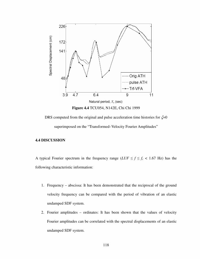
118
Natural period, Tn (sec)
Figure 4.4 TCU054, N142E, Chi Chi 1999
DRS computed from the original and pulse acceleration time histories for ζ=0
superimposed on the “Transformed–Velocity Fourier Amplitudes”
4.4 DISCUSSION
A typical Fourier spectrum in the frequency range (LUF ≤ f ≤ fc < 1.67 Hz) has the
following characteristic information:
1. Frequency – abscissa: It has been demonstrated that the reciprocal of the ground
velocity frequency can be compared with the period of vibration of an elastic
undamped SDF system.
2. Fourier amplitudes – ordinates: It has been shown that the values of velocity
Fourier amplitudes can be correlated with the spectral displacements of an elastic
undamped SDF system.
Spectr
al D
ispla
ce
me
nt
(cm
)
119
3. Gradient: It has been observed in chapter 3 that the higher the gradient of velocity
Fourier amplitudes, the greater is the dynamic amplification (Rd) of an elastic
SDF system. Steep and near-vertical velocity Fourier amplitudes relate to a higher
Rd of a SDF system. The author has not been able to establish this observation
analytically.
4. The angle of phase: Each point of the Fourier transforms (not absolute values)
defines the angle of phase. The author has not been able to uncover any relation
between this and the spectral response due to pulse.
The very important distinction between the analogous DRS and the conventional DRS is
that the former is the representation of the ground (pulse) velocity time history, whereas
the latter is the response of an elastic SDF system due to ground acceleration time history.
Analogous DRS is applicable only for the natural period of vibration, Tn greater than the
cut-off period, Tc. It has been observed that the concept presented in the present chapter
no longer holds true for periods less than the cut-off period. The transformed–Fourier
amplitudes digress rapidly from actual spectral displacements.
The analogous DRS presented in this chapter is applicable to an undamped elastic SDF
system. Can we propose any modification or a filter to the pulse-like ground velocity
time history, so that it would compute and closely represent the spectral displacements of
a SDF system with a 5% damping ratio? Since the ground cannot be dampened (recall
that the Fourier spectrum represents the frequency contents of the ground velocity time

120
history), hypothetically it may be possible to devise a synthetic filter that can be applied
to the original Fourier amplitudes, so that they subsequently have less value and have a
more or less smooth and continuous curve. We have already observed in many DRS of
ground motions with multiple period pulses that the spectral displacements for an
undamped elastic system are very uneven and erratic, whereas those for a 5% damped
system are smooth and continuous.
4.5 CONCLUSIONS
Based on the results of this study, the following conclusions can be drawn:
(1) Analogous displacement response spectrum (DRS) is a fast and efficient instrument
for understanding the spectral displacement characteristics of undamped SDF
systems. It gives the upper-bound response of structures subjected to pulse-like long-
period ground motions.
(2) Due to its inherent simplicity, the analogous DR spectrum can be used in the
preliminary stage of structural design for seismic loading.
(3) The analogous DRS could also be useful in Performance Based Seismic Design by
directly relating spectral displacements to the Fourier amplitudes of the given ground
velocity.
In chapters 2, 3 and 4, we have mostly dealt with elastic SDF systems. In the next
chapter, we will examine pulse effects on the displacement ductility requirement of an
inelastic SDF system, like a bridge bent.

121
CHAPTER 5
PULSE EFFECTS ON THE DISPLACEMENT DUCTILITY REQUIREMENT OF BRIDGE BENTS
5.1 PREVIEW
This chapter evaluates the displacement ductility requirement for a typical bridge bent
subjected to extreme loads, such as those from pulse-like near-fault ground motions
(NFGMs). The ductility requirement, as stated by prevailing design codes, may not be
valid for such structures in near-fault (less than 10 miles) zones. Due to the dominance
of the pulses, medium- to long-period structures are strongly affected, often resulting in
high residual or permanent deformations after the cessation of seismic ground motions.
As per most design codes, the magnitude of displacements associated with P-Delta
effects is required to be captured using non-linear time history analysis. The higher the
value of the target displacement ductility demand or the P-Delta ratio, the larger is the
magnitude of the residual displacements. Because permanent deformations in a bridge
bent would lead to a higher eccentric loading from the superstructure, the bent would be
subjected to higher secondary moments from it own design load. Even if the bridge
survives the earthquake, subsequent failure may occur due to its own design loads. A
suitable balance should be made between ductility and residual displacements in the
design of such structures using Performance-Based Seismic Design procedures.

122
5.2 INTRODUCTION
Performance-Based Seismic Design (PBSD) is a process that permits the design of new
structures or the upgrade of existing structures with a realistic understanding of the risk of
life, as well as occupancy and economic losses that may occur as a result of earthquakes.
The performance of a structure designed using PBSD is studied after it is subjected to
various earthquake events. Each study provides valuable information on the level of
damage, which consequently allows us to estimate the amount of life, occupancy and
economic losses that may occur. The design can be adjusted until the projected risks or
losses are acceptable. The Applied Technology Council (ATC), under FEMA
sponsorship, is currently engaged in a project (ATC-58) to develop the next-generation
PBSD procedures and guidelines. [FEMA-445 2006]
Long-period ground motions that give rise to directivity or path effects are important
seismic design considerations because they often impose large demands on medium to
long-period structures. The inherent properties that cause these effects, which often
manifest themselves as pulses, have been identified as dominant low-frequency contents
embedded in typical long-period seismic ground motions [Khanse and Lui 2008a; 2008b;
2009].
As per CALTRANS (2006) Seismic Design Criteria (SDC), v 1:4 the target global
displacement ductility demand value µD for single column bents supported on fixed
foundation should be ≤ 4. Further, CALTRANS SDC requires that the dynamic effects of
gravity loads acting through lateral displacements shall be included in the design; and

123
that the magnitude of displacements associated with P-Delta effects can only be
accurately captured with non-linear time history analysis.
This chapter examines the existing provisions for ductility requirements for a typical
bridge bent subjected to seismic ground motions, and demonstrates that these ductility
requirements may not be valid for structures in near-fault (< 10 miles) zones. Due to
dominance of the pulses, structures having a natural period of vibration Tn between 1 and
2 seconds are highly affected, often resulting in high residual displacements (or
permanent deformations) even after the cessation of seismic ground motions. Although
the existing design codes do not specify the extent of permissible permanent
displacements/ deformations, it is clear that a higher target local displacement ductility
demand value µC will result in larger residual displacements, which may not be desirable.
A suitable balance should therefore be made for the design of structures, like single
column bents in near-fault zones using Performance-Based Seismic Design
methodologies.
Appendix C of ATC-55 [FEMA-440 2005] gives plots of CR values (i.e., the ratio of
maximum nonlinear to linear displacements) versus periods of vibration in Sec. C.2.1 and
C.2.2 for the elastic perfectly plastic (EPP) and the stiffness-degrading (SD) hysteretic
models, respectively. Although this critical parameter is important for the design of a
system undergoing seismic excitation (i.e., during an earthquake), the effect of permanent
deformations after cessation of the earthquake is another criterion that needs to be

124
addressed, especially if the permanent deformations are excessive. This chapter intends
to shed light on this aspect of seismic design.
5.3 EXISTING DESIGN CODE PROVISIONS FOR
DISPLACEMENT DUCTILITY DEMAND VALUE, µC
5.3.1 CALTRANS Seismic Design Criteria, 2006, v 1:4 [CALTRANS 2006]
CALSTRANS SDC is focused on concrete bridges. An individual bent or column has
been referred to as a local system. Displacement ductility demand is a measure of the
imposed post-elastic deformation on a member. As per Sec. 2.2.4, the target global
displacement ductility demand value for Single Column Bents supported on fixed
foundation is µD ≤ 4. The target value may range between 1.5 and 3.5 where specific
values cannot be defined. Local displacement ductility capacity for a cantilever column
fixed at the support (Fig. 5.1) is defined by Eq. 3.6 of SDC as:
CC col
y
∆µ
∆= (5.1)
col
y∆ is shown in Fig. 5.1. Local member displacement capacity C
∆ is defined as a
member’s displacement capacity attributed to its elastic and plastic flexibility as defined
in SDC Sec. 3.1.4. The structural system’s displacement capacity C
∆ is the reliable lateral
capacity of the bridge or subsystem as it approaches its collapse limit state. Further, SDC
Sec. # 3.1.4.1 states that each ductile member shall have a minimum local displacement
ductility capacity of µC = 3 to ensure dependable rotational capacity in the plastic hinge

125
regions regardless of the displacement demand imparted to that member. If µC < 3,
approval from competent authority is required.
Figure 5.1. Local Displacement Capacity - Cantilever Column w/ Fixed Base (left)
P-Delta Effects on Bridge Columns [Fig. 3.1 & 4.2 from CALTRANS 2006]
Sec. 4.2 of SDC on P-Delta Effects states that (1) The dynamic effects of gravity loads
acting through lateral displacements shall be included in the design, and (2) The
magnitude of displacements associated with P-Delta effects can only be accurately
captured with non-linear time history analysis.
Sec. 6.1.2.1 of SDC states that for preliminary design of structures within 10 miles of an
active fault, the spectral acceleration on the Acceleration Response Spectrum (ARS)
curves shall be magnified by 20% for Tn≥1.0 sec., and a linear interpolation from 0 to
20% be used for 0.5≤Tn≤1.0 sec.
5.3.2 AASHTO (2007, 2009) Guide Specifications for LRFD Seismic Bridge Design

126
AASHTO (2007) Sec. C4.2.2 states that essential or critical bridges within 6 miles of an
active fault require a site-specific study and inclusion of vertical ground motion in the
seismic analysis. As per Sec. 4.7.1 on ‘Design Methods for Lateral Seismic Displacement
Demands’, each structure shall be categorized according to its intended structural seismic
response in terms of damage levels:
a) Conventional Ductile Response (i.e., Full-Ductility Structures): 4.0 ≤ µD ≤ 6.0,
(see Article 4.9 of AASHTO 2007). This response is anticipated for a bridge in
Seismic Design Category D designed for the Life Safety Criteria.
b) Limited-Ductility Response for horizontal loading, local µD < 4.
c) Limited-Ductility Response in concert with added protective systems. In this case
a structure has limited ductility with the additional seismic isolation, passive
energy dissipating devices, and/or other mechanical devices to control seismic
response. Using this strategy, a plastic mechanism may or may not form. µD is the
local displacement ductility demand in AASHTO 2007.
AASHTO 2007 Sec. C4.7.1 states that design displacements and minimum flexural
capacities of columns are generally governed by P-Delta effects. Sec. 4.9 on Member
ductility requirement for Seismic Design Category D states that for single column bents,
local member ductility demand µD ≤ 5. Sec. 4.11.5 on ‘P-Delta Capacity Requirement
for Seismic Design Category C and D’ requires that the dynamic effects of gravity loads
acting through lateral displacements shall be included in the design. The magnitude of
displacements associated with P-Delta effects can only be accurately captured with non-
linear time history analysis.

127
5.4 BRIEF BACKGROUND
After a system yields, it goes into the inelastic stage. Behavior of a typical steel single
degree-of-freedom (SDF) system may be represented by an Elasto-plastic (EP) force-
deformation model as shown in Fig. 5.2. In the present analysis using BISPEC, the
Elasto-perfectly-plastic (EPP) model (Fig. 5.2.a) is used. However, a more general
version is the bi-linear model shown in Fig. 5.2.b in which the post-yield stiffness k1 is
not zero.
On the other hand, the behavior of a typical concrete SDF system in the inelastic stage is
usually idealized by the stiffness degrading (SD) model as shown in Fig. 5.3. In this
model, Initial Yield Point (IYP) and Current Yield Point (CYP) as marked on Fig. 5.3 are
required to determine subsequent stiffness after unloading or reloading. In the present
analysis using BISPEC, the ordinary stiffness degrading (SD) model is used for the
response evaluation.
The governing equation for a system that experiences inelastic behavior is
( , ) ( )s
mu cu f u u ma t+ + = −&& & &
For a given ground acceleration time history a(t), u(t) depends on ωn, ζ and uy in addition
to the form of the hysteretic force-deformation relation used as illustrated in Fig. 5.2 or
5.3.
As defined on Fig. 5.2.a, the ductility factor is given by
m
y
u
uµ =

128
Another factor that is of interest in an inelastic analysis is the yield strength ratio, given
by β = fy/(mg), where fy is the yield force, m is the mass of the system, and g is the
acceleration due to gravity.
Figure 5.2. Idealized Elasto-Plastic behavior:
(a) Elasto-perfectly-plastic (EPP) model, (b) Bilinear Elasto-plastic model [Clough 1966]
Figure 5.3. Idealized Stiffness Degrading (SD) behavior:
(a) Ordinary SD model, (b) Bilinear SD model [Clough 1966]
As per ATC-55 (FEMA 440), CR is a modification factor to relate the expected maximum
displacement of an inelastic SDF system with EPP or SD hysteretic properties to
displacements calculated for the linear elastic response. A plot of CR against period of
vibration for an EPP model is shown in Fig. 5.4 for first 20 NFGM as listed in Table 5.5.
Fig. 5.5 exhibits a plot of CR for the SD model. The plots are given for different values of
fy
fs fs
fy
fs fs
fy

129
normalized lateral strength, R = (mSa)/fy; where m is the mass of SDF system, and Sa is
the spectral acceleration. (mSa) is the elastic strength demand, and fy is the yield force.
Figure 5.4. CR values of SDF system having ζ = 0.05 with Elasto-perfectly Plastic (EPP)
hysteretic behavior for a set of 20 NFGM as given in Table 5.5 [Sec. C.2.1 of ATC-55]
Figure 5.5. CR values of SDF system having ζ = 0.05 with stiffness degrading (SD)
hysteretic behavior for a set of 20 NFGM as given in Table 5.5 [Sec. C.2.2 of ATC-55]

130
Time (sec)
While the importance of CR values in the analyses cannot be overemphasized, the
residual displacements (permanent deformation) of an inelastic system after cessation of
pulse-like near-fault ground motions (NFGMs) is another critical parameter that needs to
be addressed.
For example, consider a bridge bent modeled as an ordinary stiffness degrading (SD)
SDF system with ζ = 0.05 having height L = 30 ft, m = 5 kip-sec2/in and a natural period
of vibration, Tn = 1.2 sec. (This value of Tn is selected because the period of one of the
pulses of ground ATH used in this example is 1.2 sec.). From k = mω2, we have k = 137
kip/in. To obtain µ = 4, fy was (iteratively) determined to be 1050 kips. Thus, uy = fy/k =
7.6 in ≈ L/50 = 7.2 in. When such a system is subjected to a pulse-like ground motion
such as Takatori, Kobe 1995, a displacement response plot as shown in Fig. 5.8 is
obtained. From the figure it can be seen that the maximum inelastic displacement is, um =
31.5 in, and that after cessation of ground motions a permanent deformation (residual
displacement) of 11.7 inches remains. This residual displacement is considered quite high
for the 30-ft bridge bent. 31.5 137
41050
m m
y y
u u k
u fµ
×= = = ≈
Figure 5.6. Displacement response of a SDF system subjected to Takatori, Kobe 1995
Dis
pla
cem
ent
(in
)

131
The present research work addresses the probable (mean + one standard deviation) values
of residual displacements for SDF system for different groups of pulse-like ground
motions. This area has not been addressed in prevailing codes including CALTRANS
SDC 2006.
5.5 EVALUATION PROCEDURES
This chapter examines the effect of variation in residual displacements (permanent
deformations) on a single degree-of-freedom system after cessation of near-fault pulse-
like ground motions. A bridge bent or column can be modeled as a single degree-of-
freedom system since most of its mass is concentrated at the top free end (Fig. 5.1). The
support at the bottom is assumed fixed, i.e., ground rotation is neglected. Further, the
effect of near-fault vertical ground motions is neglected. These two would likely
aggravate the values of residual displacements after cessation of ground motions. Five
groups of pulse-like near-fault ground motion records with forward directivity are
considered:
(1) Mw = 6.5 ± 0.25, Soil = A & B, 8 records (Table 5.1)
(2) Mw = 6.5 ± 0.25, Soil = D, 19 records (Table 5.2)
(3) Mw = 7.25 ± 0.25, Soil = A & B, 12 records (Table 5.3)
(4) Mw = 7.25 ± 0.25, Soil = D, 15 records (Table 5.4)
(5) ATC-55 (2005), 6.19 ≤ Mw ≤ 7.62, Soil = A, B, D & E, (20 + 2) records (Table 5.5)

132
Table 5.1. Mw = 6.5 ± 0.25, Soil = A & B
No Soil File NGA R
(miles)
PGA
(g)
PGV
(in/s)
PGD
(in)
1 A NORTHR_655_032FN 0983 3.37 0.52 26.5 16.8
2 A NORTHR_LDM_032FN 1013 3.67 0.58 30.3 7.9
3 A NORTHR_PUL_032FN 1051 4.35 1.38 42.1 8.9
4 A NORTHR_PAC_032FN 1050 4.35 0.50 19.3 2.5
5 B NORTHR_SCE_032FN 1085 3.22 0.84 45.8 15.5
6 B NORTHR_JEN_032FN 0982 3.37 0.52 26.5 16.5
7 B NORTHR_WPI_032FN 1045 3.4 0.43 34.5 21.7
8 B NORTHR_RRS_032FN 1063 4.03 0.87 65.7 11.3
Table 5.2. Mw = 6.5 ± 0.25, Soil = D
No Soil File NGA R
(miles)
PGA
(g)
PGV
(in/s)
PGD
(in)
1 D IMPVALL_HEMO_233FN 171 0.04 0.38 45.3 15.8
2 D IMPVALL_HAEP_233FN 158 0.21 0.36 17.4 4.1
3 D IMPVALL_HE07_233FN 181 0.35 0.46 42.83 18.0
4 D IMPVALL_HAGR_233FN 159 0.40 0.31 21.2 6.0
5 D IMPVALL_HE06_233FN 181 0.77 0.44 44.0 26.2
6 D IMPVALL_HE08_233FN 183 2.39 0.47 19.1 14.5
7 D IMPVALL_HE05_233FN 180 2.45 0.38 36.0 24.4
8 D IMPVALL_HEDA_233FN 184 3.15 0.42 23.5 15.3
9 D NORTHR_SYL_032FN 1086 3.29 0.73 48.3 12.4
10 D NORTHR_SCS_032FN 1084 3.32 0.59 51.3 21.3
11 D NORTHR_NWH_032FN 1044 3.67 0.72 47.3 13.8
12 D IMPVALL_HE10_233FN 173 3.83 0.18 18.5 12.4
13 D IMPVALL_HE04_233FN 179 4.37 0.36 30.6 23.1
14 D IMPVALL_HECC_233FN 170 4.53 0.18 21.5 15.1
15 D IMPVALL_HHVP_233FN 185 4.74 0.26 21.7 13.0
16 D NORTHR_0637_032FN 1004 5.23 0.73 24.9 7.4
17 D IMPVALL_HE11_233FN 174 7.72 0.37 16.2 7.3
18 D IMPVALL_HE03_233FN 178 7.97 0.23 16.2 9.3
19 D NORTHR_CNP_032FN 0959 9.11 0.38 21.1 8.5
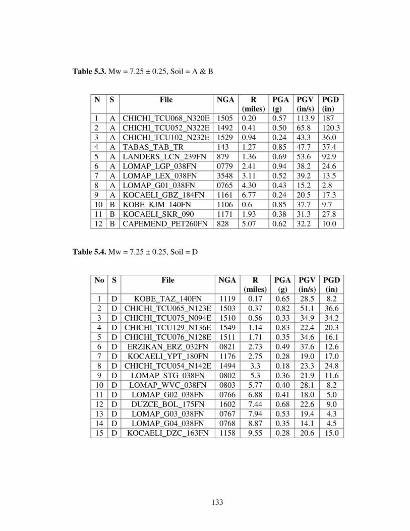
133
Table 5.3. Mw = 7.25 ± 0.25, Soil = A & B
N S File NGA R
(miles)
PGA
(g)
PGV
(in/s)
PGD
(in)
1 A CHICHI_TCU068_N320E 1505 0.20 0.57 113.9 187
2 A CHICHI_TCU052_N322E 1492 0.41 0.50 65.8 120.3
3 A CHICHI_TCU102_N232E 1529 0.94 0.24 43.3 36.0
4 A TABAS_TAB_TR 143 1.27 0.85 47.7 37.4
5 A LANDERS_LCN_239FN 879 1.36 0.69 53.6 92.9
6 A LOMAP_LGP_038FN 0779 2.41 0.94 38.2 24.6
7 A LOMAP_LEX_038FN 3548 3.11 0.52 39.2 13.5
8 A LOMAP_G01_038FN 0765 4.30 0.43 15.2 2.8
9 A KOCAELI_GBZ_184FN 1161 6.77 0.24 20.5 17.3
10 B KOBE_KJM_140FN 1106 0.6 0.85 37.7 9.7
11 B KOCAELI_SKR_090 1171 1.93 0.38 31.3 27.8
12 B CAPEMEND_PET260FN 828 5.07 0.62 32.2 10.0
Table 5.4. Mw = 7.25 ± 0.25, Soil = D
No S File NGA R
(miles)
PGA
(g)
PGV
(in/s)
PGD
(in)
1 D KOBE_TAZ_140FN 1119 0.17 0.65 28.5 8.2
2 D CHICHI_TCU065_N123E 1503 0.37 0.82 51.1 36.6
3 D CHICHI_TCU075_N094E 1510 0.56 0.33 34.9 34.2
4 D CHICHI_TCU129_N136E 1549 1.14 0.83 22.4 20.3
5 D CHICHI_TCU076_N128E 1511 1.71 0.35 34.6 16.1
6 D ERZIKAN_ERZ_032FN 0821 2.73 0.49 37.6 12.6
7 D KOCAELI_YPT_180FN 1176 2.75 0.28 19.0 17.0
8 D CHICHI_TCU054_N142E 1494 3.3 0.18 23.3 24.8
9 D LOMAP_STG_038FN 0802 5.3 0.36 21.9 11.6
10 D LOMAP_WVC_038FN 0803 5.77 0.40 28.1 8.2
11 D LOMAP_G02_038FN 0766 6.88 0.41 18.0 5.0
12 D DUZCE_BOL_175FN 1602 7.44 0.68 22.6 9.0
13 D LOMAP_G03_038FN 0767 7.94 0.53 19.4 4.3
14 D LOMAP_G04_038FN 0768 8.87 0.35 14.1 4.5
15 D KOCAELI_DZC_163FN 1158 9.55 0.28 20.6 15.0
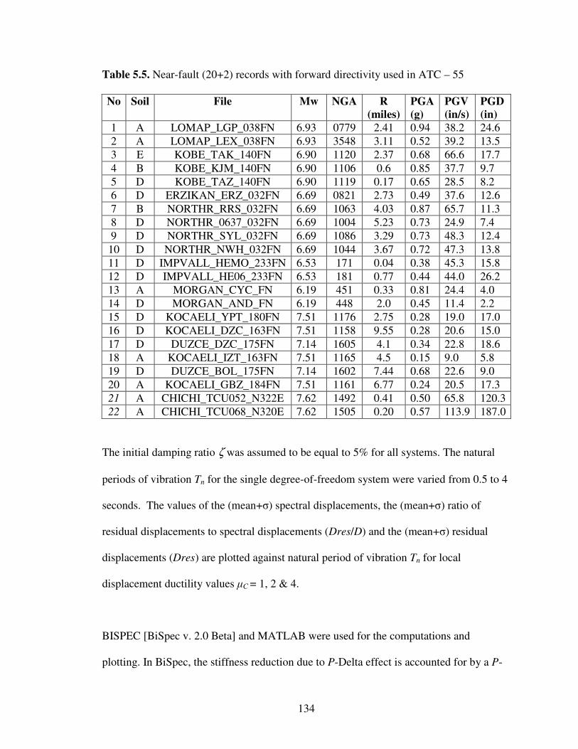
134
Table 5.5. Near-fault (20+2) records with forward directivity used in ATC – 55
No Soil File Mw NGA R
(miles)
PGA
(g)
PGV
(in/s)
PGD
(in)
1 A LOMAP_LGP_038FN 6.93 0779 2.41 0.94 38.2 24.6
2 A LOMAP_LEX_038FN 6.93 3548 3.11 0.52 39.2 13.5
3 E KOBE_TAK_140FN 6.90 1120 2.37 0.68 66.6 17.7
4 B KOBE_KJM_140FN 6.90 1106 0.6 0.85 37.7 9.7
5 D KOBE_TAZ_140FN 6.90 1119 0.17 0.65 28.5 8.2
6 D ERZIKAN_ERZ_032FN 6.69 0821 2.73 0.49 37.6 12.6
7 B NORTHR_RRS_032FN 6.69 1063 4.03 0.87 65.7 11.3
8 D NORTHR_0637_032FN 6.69 1004 5.23 0.73 24.9 7.4
9 D NORTHR_SYL_032FN 6.69 1086 3.29 0.73 48.3 12.4
10 D NORTHR_NWH_032FN 6.69 1044 3.67 0.72 47.3 13.8
11 D IMPVALL_HEMO_233FN 6.53 171 0.04 0.38 45.3 15.8
12 D IMPVALL_HE06_233FN 6.53 181 0.77 0.44 44.0 26.2
13 A MORGAN_CYC_FN 6.19 451 0.33 0.81 24.4 4.0
14 D MORGAN_AND_FN 6.19 448 2.0 0.45 11.4 2.2
15 D KOCAELI_YPT_180FN 7.51 1176 2.75 0.28 19.0 17.0
16 D KOCAELI_DZC_163FN 7.51 1158 9.55 0.28 20.6 15.0
17 D DUZCE_DZC_175FN 7.14 1605 4.1 0.34 22.8 18.6
18 A KOCAELI_IZT_163FN 7.51 1165 4.5 0.15 9.0 5.8
19 D DUZCE_BOL_175FN 7.14 1602 7.44 0.68 22.6 9.0
20 A KOCAELI_GBZ_184FN 7.51 1161 6.77 0.24 20.5 17.3
21 A CHICHI_TCU052_N322E 7.62 1492 0.41 0.50 65.8 120.3
22 A CHICHI_TCU068_N320E 7.62 1505 0.20 0.57 113.9 187.0
The initial damping ratio ζ was assumed to be equal to 5% for all systems. The natural
periods of vibration Tn for the single degree-of-freedom system were varied from 0.5 to 4
seconds. The values of the (mean+σ) spectral displacements, the (mean+σ) ratio of
residual displacements to spectral displacements (Dres/D) and the (mean+σ) residual
displacements (Dres) are plotted against natural period of vibration Tn for local
displacement ductility values µC = 1, 2 & 4.
BISPEC [BiSpec v. 2.0 Beta] and MATLAB were used for the computations and
plotting. In BiSpec, the stiffness reduction due to P-Delta effect is accounted for by a P-

135
Delta (pd) ratio, defined as (P/L)/K that varies from 0 to 1. In the equation K is the gross
stiffness of the system, P in this case is Pdl, and L is the height of the SDF system as
shown in Fig. 5.1. The Stiffness Degradation (SD) model with two different pd ratios (0
and 0.05) were used in the analysis for the first four sets (i.e., Groups 1, 2, 3 & 4) of
ground motions. BISPEC gives data output in US systems, therefore US system of
measurements are used in this chapter.
The first twenty ground motion records of group No. 5 were taken from Appendix C of
ATC-55 [FEMA-440 2005]. Since the original list did not contain any record from the
Chi-Chi earthquake, two records have been added to make the total of twenty-two. Two
different hysteretic models, the stiffness-degrading (SD) model and the elastic perfectly
plastic (EPP) model, and three pd ratios (0, 0.05, 0.1) were used in the analysis for this
set of ground motions.
5.6 PARAMETRIC STUDY
In Appendix B of the Seismic Design Criteria (SDC), Acceleration Response Spectra
(ARS) curves have been drawn as per the earthquake magnitude (Mw) and soil profile
type for SDF system having damping ratio 5%. Similar sub-divisions are made from
known pulse-like ground motion records having forward directivity. The fault-normal
components of these records are given in Tables 5.1 to 5.4, which have been used in the
parametric computations. An effort is made to determine if there is a relationship between
the residual displacement Dres and the spectral displacement D at a given natural period
of vibration Tn.

136
For Groups 1 and 2, it is observed from Fig. 5.7.a and 5.8.a that the mean+σ spectral
displacements for µc = 1, 2 & 4 begin to deviate from one another when Tn = 2.5 sec.
From Fig. 5.7.b, it is observed that the mean+σ Dres/D ratios remain more or less
constant for Tn = 0.5 to 4 seconds. However, a small variation in P-Delta (pd) ratio from
0 to 0.05 results in a considerable increase (from an average of 0.36 to 0.75) in Dres/D
for µC = 4, although the effect is less pronounced (from an average of 0.21 to 0.38) for µC
= 2. Similar trend and values for Dres/D are observed for ground motions in Group 2 for
soil profile type D, as seen from Fig. 5.8.b. Thus, a change in soil profile type does not
seem to have an appreciable effect on Dres/D.

137
Natural period, n
T (sec)
Natural period, n
T (sec)
Figure 5.7. Group 1, SD Model, Mw = 6.5 ± 0.25, Soil Type A, B
(a) the (mean+σ) Displacement Response Spectrum
(b) the (mean+σ) Residual Displacement/Spectral Displacement Spectrum
Sp
ectr
al D
isp
lace
men
t (i
n)
Dre
s /
Sp
ectr
al D
isp
µC = 1
µC = 2
µC = 4
µC = 2, pd=0
µC = 2, pd=.05
µC = 4, pd=0
µC = 4, pd=.05
(a)
(b)
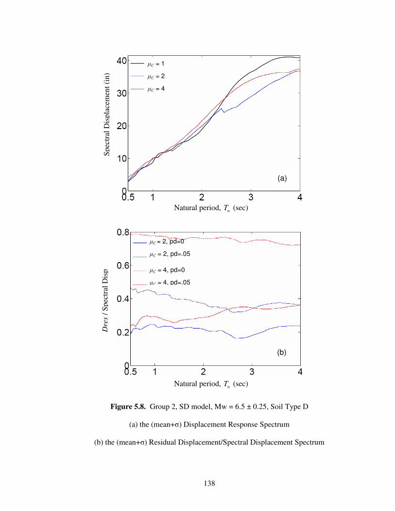
138
Natural period, n
T (sec)
Natural period, n
T (sec)
Figure 5.8. Group 2, SD model, Mw = 6.5 ± 0.25, Soil Type D
(a) the (mean+σ) Displacement Response Spectrum
(b) the (mean+σ) Residual Displacement/Spectral Displacement Spectrum
Sp
ectr
al D
isp
lace
men
t (i
n)
Dre
s /
Sp
ectr
al D
isp
µC = 1
µC = 2
µC = 4
µC = 2, pd=0
µC = 2, pd=.05
µC = 4, pd=0
µC = 4, pd=.05
(b)
(a)

139
For Group 3 and 4, it is observed from Fig. 5.9.a and 5.10.a that the mean+σ spectral
displacements for µC = 1, 2 & 4 are quite comparable. From Fig. 5.9.b, it is observed that
the mean+σ Dres/D ratios remain more or less constant for µC = 2 and 4. A small
variation in pd ratio from 0 to 0.05 results in a considerable increase (from an average of
0.30 to 0.74) in Dres/D for µC = 4, although the effect is less pronounced (from an
average of 0.22 to 0.39) for µC = 2. Similar trends and values for Dres/D are observed for
ground motions in Group 4 for soil profile type D, as seen from Fig. 5.10.b. Thus, a
change in soil profile type does not seem to have an appreciable effect on Dres/D.

140
Natural period, n
T (sec)
Natural period, n
T (sec)
Figure 5.9. Group 3, SD model, Mw =7.25 ± 0.25, Soil Type A, B
(a) the (mean+σ) Displacement Response Spectrum,
(b) the (mean+σ) Residual Displacement/Spectral Displacement Spectrum
Sp
ectr
al D
isp
lace
men
t (i
n)
Dre
s /
Sp
ectr
al D
isp
µC = 1
µC = 2
µC = 4
µC = 2, pd=0
µC = 2, pd=.05
µC = 4, pd=0
µC = 4, pd=.05
(b)
(a)

141
Natural period, n
T (sec)
Natural period, n
T (sec)
Natural period, n
T (sec)
Figure 5.10. Group 4, SD model, Mw = 7.25 ± 0.25, Soil Type D
(a) the (mean+σ) Displacement Response Spectrum
(b) the (mean+σ) Residual Displacement/Spectral Displacement Spectrum
Sp
ectr
al D
isp
lace
men
t (i
n)
Dre
s /
Sp
ectr
al D
isp
µC = 1
µC = 2
µC = 4
µC = 2, pd=0
µC = 2, pd=.05
µC = 4, pd=0
µC = 4, pd=.05
(b)
(a)

142
It is pertinent here to observe the effect of the record Takatori, Kobe 1995 earthquake
(KOBE_TAK_140FN, soil-type E) on the spectral displacements and residual
displacements. We do not have any other pulse-like record of stations on E-type soil. Fig.
5.11.a illustrates the spectral distances plotted against the period of vibration, Tn. From
the figure it may be observed that the spectral displacements are very high for a period of
vibration 1 to 2.5 sec. From Fig. 5.11.b it may be observed that for µC = 2, Dres/D are
high around 0.4 to 0.5, for pd = 0.05 and 0.1. For µC = 4, they are very high around 0.8
for pd=0.05 and 0.1. High ductile ratio of µC = 4 has a disastrous effect on structures near
this station. Similar observation can be made from Fig. 5.11.c, which shows the residual
displacements for stiffness degrading (SD) model, for pd = 0, 0.05 and 0.1.

143
(a)
(b)
Natural period, n
T (sec)
Natural period, n
T (sec)
Sp
ectr
al D
isp
lace
men
t (i
n)
Dre
s /
Sp
ectr
al D
isp
µC = 1
µC = 2
µC = 4
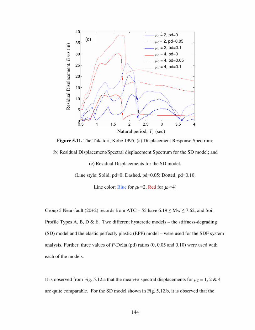
144
Figure 5.11. The Takatori, Kobe 1995, (a) Displacement Response Spectrum;
(b) Residual Displacement/Spectral displacement Spectrum for the SD model; and
(c) Residual Displacements for the SD model.
(Line style: Solid, pd=0; Dashed, pd=0.05; Dotted, pd=0.10.
Line color: Blue for µC=2, Red for µC=4)
Group 5 Near-fault (20+2) records from ATC – 55 have 6.19 ≤ Mw ≤ 7.62, and Soil
Profile Types A, B, D & E. Two different hysteretic models – the stiffness-degrading
(SD) model and the elastic perfectly plastic (EPP) model – were used for the SDF system
analysis. Further, three values of P-Delta (pd) ratios (0, 0.05 and 0.10) were used with
each of the models.
It is observed from Fig. 5.12.a that the mean+σ spectral displacements for µC = 1, 2 & 4
are quite comparable. For the SD model shown in Fig. 5.12.b, it is observed that the
(c)
Natural period, n
T (sec)
Res
idu
al D
isp
lace
men
t, D
res
(in
)
µC = 2, pd=0
µC = 2, pd=0.05
µC = 2, pd=0.1
µC = 4, pd=0
µC = 4, pd=0.05
µC = 4, pd=0.1
145
mean+σ Dres/D ratios remain more or less constant for µC = 2 and 4. For µC = 2, the
average Dres/D values are 0.21, 0.38 and 0.58 for pd ratios of 0, 0.05 and 0.10,
respectively. As has previously been observed, a small variation in pd ratio from 0 to
0.05 results in a considerable increase (from an average of 0.30 to 0.74) in Dres/D for µC
= 4, although the effect is less drastic (from an average of 0.74 to 0.82) for µC = 2.
For the EPP model (Fig. 5.12.c) the variation in Dres/D is rather erratic; however, since
the trend is more or less horizontal, the average values of Dres/D for µC = 2 can be
computed as 0.38, 0.44 and 0.5 for pd ratios of 0, 0.05 and 0.10, respectively. The
average values of Dres/D for µC = 4 are 0.51, 0.7 and 0.8 for pd ratios of 0, 0.05 and 0.10.
Because residual displacements computed using the EPP model are higher than those
computed using the SD model, the use of materials that can be modeled using the SD
model (such as concrete) is more preferable for use as bridge bents. This observation is
reinforced in Figures 5.13 and 5.14 in which residual displacement values Dres are
plotted for both the SD and EPP models over a range of Tn from 0.5 to 4.

146
Natural period, n
T (sec)
Natural period, n
T (sec)
Sp
ectr
al D
isp
lace
men
t (i
n)
Dre
s /
Sp
ectr
al D
isp
µC = 1
µC = 2
µC = 4
(b)
(a)
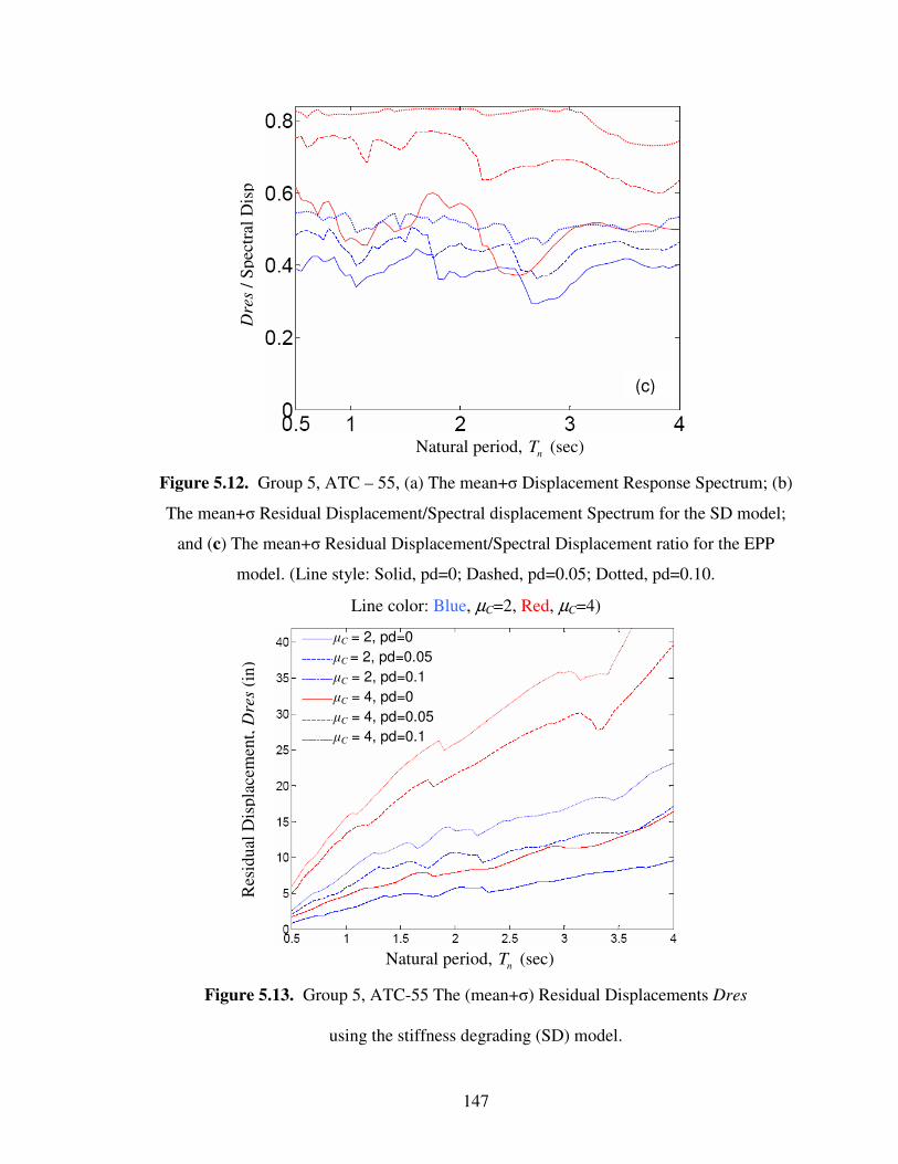
147
Natural period, n
T (sec)
Natural period, n
T (sec)
Figure 5.12. Group 5, ATC – 55, (a) The mean+σ Displacement Response Spectrum; (b)
The mean+σ Residual Displacement/Spectral displacement Spectrum for the SD model;
and (c) The mean+σ Residual Displacement/Spectral Displacement ratio for the EPP
model. (Line style: Solid, pd=0; Dashed, pd=0.05; Dotted, pd=0.10.
Line color: Blue, µC=2, Red, µC=4)
Figure 5.13. Group 5, ATC-55 The (mean+σ) Residual Displacements Dres
using the stiffness degrading (SD) model.
Dre
s /
Sp
ectr
al D
isp
Res
idu
al D
isp
lace
men
t, D
res
(in
)
µC = 2, pd=0
µC = 2, pd=0.05
µC = 2, pd=0.1
µC = 4, pd=0
µC = 4, pd=0.05
µC = 4, pd=0.1
(c)

148
Natural period, n
T (sec)
Figure 5.14. Group 5, ATC – 55 The (mean+σ) Residual Displacements Dres
using the elastic perfectly plastic (EPP) model.
5.7 DISCUSSION
For structures such as a bridge bent or bridge-column in an active near-fault zone (less
than 10 miles from fault-rupture planes), the permissible limit on the target displacement
ductility to ensure that the amount of residual displacements will not be excessive after
cessation of ground motions is currently not adequately addressed in a number of seismic
design provisions.
Using the minimum local displacement ductility requirement of µc = 3 as per SDC Sec.
3.1.4.1 may not be advisable for such structures in near-fault zones. As per Sec. 4.2 of
SDC, the dynamic effects of gravity loads acting through the lateral displacements shall
Res
idu
al D
isp
lace
men
t, D
res
(in
)
µC = 2, pd=0
µC = 2, pd=0.05
µC = 2, pd=0.1
µC = 4, pd=0
µC = 4, pd=0.05
µC = 4, pd=0.1

149
be included in the analysis. From Fig. 5.13, it is observed that for systems that exhibit
the stiffness degrading (SD) behavior (e.g., a concrete bent) with a pd ratio of 0.05 and µc
= 2, the residual displacement, Dres varies from 5 in. (for Tn = 1 sec.) to 10 in. (for Tn = 2
sec.); and for µc = 4 and a pd ratio of 0.05, Dres varies from 12 in. (for Tn = 1 sec.) to 20
in. (for Tn = 2 sec.). The residual displacements will be more pronounced for a higher pd
ratio. Given this observation, the question that needs to be answered is what should the
range of permissible µc be, if residual displacements are to be limited?
In a Performance-Based Seismic Design (PBSD) procedure, structural performance is
communicated by reference to a series of standard performance levels that range from
states of negligible damage and impact on safety, occupancy and use to states of near
complete damage in which there is extensive risk to life, complete loss of economic value
and permanent loss of use and function. Under these procedures, decision makers must
select the desired performance levels (e.g., fully functional, immediate occupancy, life
safety, collapse prevention), and the earthquakes for which these performance levels are
to be achieved. Decision makers should be able to define these risks in terms of the future
life loss, facility repair costs and downtime that could result from design decisions.
[FEMA-445 2006]
The design of structures at fully functional or immediate occupancy level should be more
stringent. In order to avoid permanent deformations, a stronger and stiffer structure
having a lower target displacement ductility value may be desired. Plots similar to Fig.
150
5.13 and 5.14 would be useful in determining the target residual displacements and
displacement ductility.
For life safety or collapse prevention level, adaption of higher displacement ductility may
result in higher permanent deformations. These higher permanent deformations, when
coupled with an increase in the P-Delta ratio due to a possible reduction in gross stiffness
from cracked sections after the quake, may cause the bridge bent to be subjected to a
higher eccentric loading from the superstructure, which is not desirable.
5.8 SUMMARY AND CONCLUSIONS
In this chapter, existing provisions for ductility requirements for a typical bridge pier or
bent subjected to seismic loading were briefly discussed. These provisions were applied
to cases in which the structure was subjected to extreme loads such as pulse-like near-
fault ground motions. A bridge bent, modeled as a SDF system, is subjected to different
groups of pulse-like near-fault ground motion records. As expected, higher residual
displacements are observed with an increase in displacement ductility or P-Delta ratio.
The investigation of the residual displacement response of an inelastic SDF system
subjected to different groups of pulse-type near-fault ground motions has led to the
following observations:
1) The spectral displacements do not seem to vary appreciably with different µC
values for Tn = 0.5 to 4 sec. (Figs. 5.8.a, 5.9.a, 5.10.a and 5.12.a)

151
2) The ratio Dres/D (where D is the spectral displacement) remains more or less
constant from Tn = 0.5 to 4 sec. for a constant displacement ductility or P-Delta
ratio (Fig. 5.7.b, 5.8.b, 5.9.b, 5.10.b and 5.12.b)
3) Residual displacements are higher for systems modeled using the EPP hysteretic
model (such as steel) as shown in Fig. 5.14 than for systems modeled by the SD
hysteretic model (such as concrete) as shown in Figure 5.13. Therefore, the use of
concrete is more preferable whenever it is possible.
4) Because of the relatively high residual displacements (Figs. 5.13 & 5.14) for a
nominal P-Delta ratio of 0.05, the target displacement ductility may need to be
restricted between 2 to 3. .
This restriction may not ensure a dependable rotational capacity in regions of plastic
hinge. Failure may be sudden if the actual pulse-like ground motion exceeds the design
excitation. A higher factor of safety may have to be adopted for design of such structures
in near-fault zone.

152
CHAPTER 6
SUMMARY AND
CONCLUSIONS
The major objective of the study presented in this dissertation is to develop a basic
understanding of the characteristics of pulse-like near-fault ground motions (NFGM) and
its impact on the response characteristics of a single degree-of-freedom (SDF) system.
The excitation properties intrinsic to pulses are inherently different from non-pulse type
seismic ground motions. They may affect medium to large period structures often
resulting in excessive displacements during the earthquake or permanent deformations
after the cessation of earthquake.
6.1 EXTRACTION OF ACCELERATION AND VELOCITY PULSE/S
In most research, velocity pulse shapes (triangular, sinusoidal, rectangular, etc.) were
assumed as best-fit to velocity time history (VTH). It is then differentiated to obtain the
acceleration pulse. An important difference between the proposed approach and those of
the other researchers is that no predetermined pulse shape is assumed in this analysis.
The natural shape and duration of the pulses are extracted directly from processed ground
motion records. These extracted pulses are then used to determine their effects on SDF
systems.

153
For the extracted pulses to be close to ‘real’ pulses, it is essential that the response due to
the pulse should be as close to the response due to original acceleration time history
(ATH) as possible. By using only the pulse component of the ground motion as the
excitation force, it is shown in this work that the displacement response of the SDF
system with a natural period exceeding a certain value referred to as the cut-off period Tc
is quite comparable with that due to the original ground excitation.
Directivity effects in ground motions can usually be detected in signal processing using
either Wavelet theory or Fourier analysis. While Wavelet theory is more useful when the
transitory characteristics or time information is more crucial in the analysis, Fourier
analysis is more appropriate when the frequency contents of the signals are of greater
importance; as in the case of directivity when a pulse might not be apparent in the
velocity time history (VTH).
It has been observed that the low-velocity soft and near-surface sediments are found to be
effective on the amplification and elongation of long-period ground motions [Hatayama
et al. 2007; Miyake and Koketsu 2007]. For most long-period ground motions records,
pulses might not be visible in VTH. Beat-phenomenon is intrinsic to the majority of
records from Japan. This phenomenon cannot be detected by Wavelet theory.
In Chapter 2, we have observed from Displacement Response Spectra (DRS) that the
high-frequency (short-period) contents of the ground motion do not appreciable affect the
displacement response of long-period systems. Recall that this non-pulse ATH is
154
obtained after the application of high-pass filter, Hhp(ω). This shows that short-period
content of time history primarily affect the response of short-period structures; whereas
long-period content of time history primarily affect the displacement response of long-
period structures.
Parseval’s Theorem and the principles of signal energy compaction were applied in pulse
extraction. In the present work it has been shown that the extracted pulse(s) indeed
contributes a large percentage of energy to the total seismic energy of near-fault ground
motions.
6.2 DISPLACEMENT RESPONSE FACTOR, Rd
In Chapter 3, it has been established that a simple sine-pulse (single period pulse) does
not always give a good representation of ground motions in response identification. The
use of a sine-pulse should be limited to those response characteristics in which the
spectral displacement more or less increases monotonically with natural period Tn from
the cut-off frequency to the frequency that corresponds to the peak of the spike nearest
the lowest usable frequency.
The pulses were qualitatively determined as (a) Monotonically increasing displacement,
which generally occurs for single period pulses, (b) Ripple effect pulses are generally the
effects of multiple period pulses, and (c) Resonance pulses are a special case of multiple

155
period pulses in which the spectral displacements are very high compared to its static
counterparts.
To quantitatively identify these three types of pulse effects, the concept of modified
Displacement Response Factor Rd was introduced.
Since short-period contents of pulse-like ground motions do not affect the displacement
response of a long-period structure, it is more rational to apply the extracted pulse on an
elastic system to determine its static displacement. In view of this, a modified
Displacement Response Factor was proposed in Chapter 3. Since the amplitude of the
pulses is much less than the Peak Ground Acceleration (PGA), the proposed dynamic
magnification factors are much larger.
A statistical study was presented in Chapter 3 on the effect of dynamic magnification
caused due to the long-period ground motions by application of modified displacement
response factor Rd. The acceleration pulses of around seventy pulse-like NFGM records
are extracted event-wise to study elastic response characteristics quantitatively by using
Rd for ζ = 0, 0.02 & 0.05.
For ζ = 0.05, the (m+σ) values of Rd varies from 3.44 to 4.8 for different earthquake
events. For pulse-like seismic ground motions the concept of equivalent harmonic forcing
frequency ratio (ω/ωn), a phase shift factor and a “damping modification factor” were
introduced in chapter 3. These concepts help us in comparing the values of dynamic

156
magnification with different earthquake events, as well as with that due to simple
harmonic excitation. Since damping controls in response characteristics of such
structures, these Rd values would assist us in the design of dampers, which could sustain
pulse-like excitations.
6.3 ANALOGOUS DISPLACEMENT RESPONSE SPECTRUM
In the fourth chapter a method for expressing spectral displacements for an undamped
linearly elastic single degree-of-freedom (SDF) system in terms of the velocity Fourier
amplitudes from the lowermost frequency range of ground motions is proposed. These
spectra, referred to as analogous displacement response spectrum (DRS), are quite
comparable to those obtained when the system is subjected to the original processed time
history or pulse-excitation. The term ‘analogous’ is used here because these spectra are
not identical to the usual DRS used in earthquake engineering design. It is essentially an
‘exact’ ground velocity Fourier amplitude plot in the lower-most frequency range (LUF ≤
f ≤ fc < 1.67 Hz) rotated about a vertical axis that passes through the cut-off frequency fc.
Because of this, the discussion is restricted to velocity Fourier amplitudes (VFA) in this
range.
The very important distinction between the analogous DRS and the conventional DRS is
that the former is the representation of the ground (pulse) velocity time history, whereas
the latter is the response of an elastic SDF system due to ground acceleration time
history.

157
Analogous displacement response spectra (DRS) are fast and efficient instruments for
understanding spectral displacement characteristics of undamped SDF systems. They
give upper-bound response of structures subjected to pulse-like long-period ground
motions.
Due to its inherent simplicity, the analogous DRS can be used in the preliminary stage of
structural design for seismic loading. The analogous DRS could also be useful in
Performance Based Design by directly relating spectral displacements to the Fourier
amplitudes of the given ground velocity.
6.4 DISPLACEMENT DUCTILITY REQUIREMENT FOR A SDF SYSTEM
The ductility requirement for a typical bridge bent subjected to extreme loads, such as
those from pulse-like near-fault ground motions (NFGMs) was examined in Chapter 5.
The ductility requirement as stated by prevailing design codes may not be valid for such
structures in near-fault (less than 10 miles) zones. Due to dominance of the pulses,
medium- to long-period structures are highly affected; often resulting in high residual or
permanent deformations after the cessation of seismic ground motions.
As per most design codes, the magnitude of displacements associated with P-Delta
effects is required to be captured using non-linear time history analysis. The higher the
158
value of the target displacement ductility demand or the P-Delta ratio, the larger is the
magnitude of the residual displacements.
A parametric study on residual deformations due to five different groups was carried out.
Residual displacements are higher for systems modeled using the EPP hysteretic model
(such as steel) than for systems modeled by the SD hysteretic model (such as concrete).
Therefore, the use of concrete is more preferable whenever it is possible.
Because of the relatively high residual displacements for a nominal P-Delta ratio of 0.05,
the target displacement ductility may need to be restricted to 2. However, this restriction
may not ensure a dependable rotational capacity in regions of plastic hinge. Failure may
be sudden if the actual pulse-like ground motion exceeds the design excitation. A higher
factor of safety may have to be adopted for design of such structures in near-fault zone.
Because of larger residual displacements after cessation of an earthquake, these
permanent deformations in a bridge bent would lead to a higher eccentric loading from
the superstructure. Subsequently, the bent would be subjected to higher secondary
moments from it own design load. Even if the bridge survives the earthquake, subsequent
failure may occur due to its own design loads. A suitable balance should be made
between ductility and residual displacements in the design of such structures.

159
6.5. SCOPE FOR FUTURE RESEARCH
Extensive research is in progress to develop simplified non-linear seismic analysis
procedures for use in performance based seismic design (PBSD). Various plots of
pseudo-spectral acceleration versus spectral displacements are being proposed for
different values of effective period (Te) and effective damping (ηeff) for a range of
ductility ratios (µ). Using Modified Acceleration Displacement Response Spectrum
(MADRS) and from the loci of performance points, the required performance point can
be selected in a performance based seismic design.
The Displacement Demand Ratio (DDR) is defined as the ratio of the maximum inelastic
spectral displacement obtained from a time history analysis to the spectral displacement
calculated from the Capacity Spectrum Method approach using the concept of equivalent
viscous damping. This ratio is used as an indicator of the validity of the equivalent
viscous damping assumption for near-field ground motions [Guyader and Iwan, 2006].
It is well-known that while structural damping does not have an appreciable effect on the
response characteristics of long-period structures subjected to non-pulse type ground
motions, it greatly affects the response of long-period structures subjected to pulse-type
ground motions. It is therefore essential that a method be developed to modify the
effective damping coefficient for structures subjected to pulse-like near-fault ground
motions.
160
Recall that as per ATC-55 (FEMA 440), CR is a modification factor to relate the expected
maximum displacement of an inelastic SDF system with EPP or SD hysteretic properties
to displacements calculated from a linear elastic response. While the importance of CR
values in the analyses cannot be overemphasized, the permanent deformation of an
inelastic system after cessation of pulse-like near-fault ground motions (NFGMs) is
another critical parameter that needs to be adequately addressed.
In essence, it is necessary to create different plots for the determination of performance
points (in PBSD) for dynamic displacements during the earthquake and for permanent
displacements after the cessation of the earthquake.
Using the minimum local displacement ductility requirement of µc = 3 as per SDC Sec.
3.1.4.1 may not be advisable for long-period structures in near-fault zones. As per Sec.
4.2 of SDC, the dynamic effects of gravity loads acting through the lateral displacements
shall be included in the p-delta analysis. In Chapter 5, it has been observed that the
residual displacements are more pronounced for a higher ductility ratio and a higher p-
delta ratio. Figure 5.13 shows that for a very nominal pd ratio of 0.05, Tn = 1 sec and µC
= 2, the residual displacement is around 5 inches. Given this observation, the question
that needs to be answered is what should the range of permissible µc be, if residual
displacements are to be limited?
The present dissertation does not contain the required parametric study to determine the
permissible range of ductility ratios for different Tn and different pd ratios, so that the

161
residual displacement is within the acceptable range. If the residual displacement is
excessive, then one would be required to change the design parameters.
A study on the effect of applied service loads on the deformed state of structures after the
cessation of earthquake should be undertaken. A concept of residual curvature may be
introduced. In p-delta analysis, the service loads (non-seismic) may be applied to the
structure (deformed) with residual curvature (from 0 degree to maybe 10 degrees). The
point of structural failure or the unacceptable deformation may be noted. Backtracking
from that point, one would be able to determine the magnitude of acceptable residual
deformation of a structure.
The most important issues to address would be (a) whether the deformed structure can
sustain the required (non-seismic) service loads, and (b) whether the deformed structure
can withstand another seismic excitation of similar or lesser magnitude? In other words,
is the reduced capacity of the structure after cessation of earthquake acceptable?
The role of suitably designed dampers should be investigated. The dampers would be
required to sustain high dynamic magnification ratio from 3.5 to 4.8 (Figure 3.19),
depending upon the location of the structure, and be able to reduce the p-delta ratio to an
acceptable value during the excitation so that the residual deformation is minimized.

162
APPENDIX
MATLAB PROGRAMMING APPLICATIONS
LIST OF PROGRAMS:
(1) Response due to half-sine pulse. Examples 5.3 & 5.4 from Text-book by Chopra, A.K
(2) Plotting Acceleration, Velocity & Displacement Response of a record
(3) Discrete Fourier Transform – Response evaluation
(4) Effect of NB on Butterworth lowpass filter
(5) Pulse, Non-pulse extraction from ATH. Energy values by Parseval Theorem
(6) Velocity (VRS) & Displacement Response Spectra (DRS) from ATH
(7) Equivalent sine-pulse, and orig-, pulse- Displacement Response Spectra
(8) Displacement Response Factor, Rd: Evaluation & plotting
(9) Analogous Displacement Response Spectra: Evaluation & plotting
(10) Half Sine Pulse – Non-linear EPP model for response evaluation

163
(1) Response due to half-sine pulse. Example 5.3 or 5.4 from Text-book by Chopra
clear all
close all
format short g
% Example 5.3 or 5.4 from Text-book by Prof. A. K. Chopra
td=0.6 % duration of applied force
To=1.2 % duration for which response is to be evaluated
dt=0.01 % time interval in second (shortened)
N=round(To/dt); % N=12
t1=[0:dt:td];
t2=[td+dt:dt:(N-1)*dt];
t=[t1 t2] % check
p1=10*sin(pi*t1/0.6); % applied loading
p2=zeros(1,size(t2,2));
p=[p1 p2]
figure
plot(t,p,'-o'); xlabel('Time (seconds)'); title('Applied Loading'); grid on
ylabel('Discrete force (kips)');
%--------------------------------------------------------------------------
% Average or Linear response analysis of SDF system by Newmark Method
m=0.2533; % kip-sec2/in (force/acceleration)
k=10; % stiffness of SDF system, units in kip/in (force/length)
c=0.1592 % damping coefficient, units in force*time/length, Ccr=2*m*wn
gamma=0.5;
beta=0.25; % beta=1/6 for linear acceleration approach
a= zeros(1,N);
v= zeros(1,N);
u= zeros(1,N);% uo, vo, ao & po have been initialized to zero.
K=k+(gamma*c)/(beta*dt)+m/(beta*dt*dt)
C1=m/(beta*dt)+gamma*c/beta
C2=m/(2*beta)+c*dt*(gamma/(2*beta)-1)
for n=1:1:N-1
dp(n)=p(n+1)-p(n);
Dp(n)=dp(n)+C1*v(n)+C2*a(n);
du(n)=Dp(n)/K;
dv(n)=gamma*du(n)/(beta*dt)-gamma*v(n)/beta+dt*a(n)*(1-gamma/(2*beta));
da(n)=du(n)/(beta*dt*dt)-v(n)/(beta*dt)-a(n)/(2*beta);
u(n+1)=u(n)+du(n);
v(n+1)=v(n)+dv(n);
a(n+1)=a(n)+da(n);
end
u

164
figure
plot(t,u); title('Response to half sine-pulse'); grid on
xlabel('Time (seconds)');ylabel('Displacement (cm)');
=============================================================
(2) Plotting Acceleration, Velocity & Displacement Response of a record
clc
clear all
format short g
%Accel, Velocity & Displacement Response of Lucerne, N239E, Landers 1992
Y = load('H:\LANDERS_LCN_260.dat');
% Accln TH accessed from PEER NGA is stored in H drive in TEXT format
N=9625 % N is the number of sample points
% Original N=9628. Accessed N points have to be multiples of 5
dt=0.005
t =[0:dt:N*dt-dt]; % time
% row by row
Yr = Y.';
in = 1;
for clm=1:1:N/5
a(in:in+4) = Yr(:,clm);
in = in + 5;
end
figure
plot(t,a);
title('ATH'); grid on
xlabel('Time in seconds');ylabel('Acceleration in g (cm/sec2)');
% Calculation of velocity & disp.
v = zeros(1,N); s = zeros(1,N);
for n = 1:1:N-1
v(n+1) = v(n) + (a(n)+ a(n+1))/2*dt; % vel
s(n+1) = s(n) + (v(n)+ v(n+1))/2*dt; % disp
end
PGV=max(abs(v*981))
PGD=max(abs(s*981))

165
figure % Velocity
plot(t,v*981);
title('VTH'); grid on
xlabel('Time in seconds');ylabel('Velocity in cm/sec');
figure % disp.
plot(t,s*981);
title('DTH'); grid on
xlabel('Time in seconds');ylabel('Displacement in cm');
=============================================================
(3) Discrete Fourier Transform – Response evaluation
clear all
close all
format short g
% Discrete FT Displacement Response to LUCERNE, N239E, LANDERS 1992
N=9625 % total number of samples of the Record - 9628
dt=0.005
SR=1/dt % SR=sampling rate
phi = 239 % Average strike-normal direction at Lucerne station is N239E
alpha = 260 % dirction of first record, N to E
beta = 345 % dirction of second record, N to E
% Above angles are in degrees each measured from N to E-direction
t =[0:dt:N*dt-dt]; % time
Y = load('H:\LANDERS_LCN_260.dat');
Yr = Y.'; % row by row
in = 1;
for clm=1:1:N/5;
a(in:in+4) = Yr(:,clm);
in = in + 5;
end
a1=[0 a]; % Initializing acceleration to zero
Y = load('H:\LANDERS_LCN_345.dat');
Yr = Y.';
a = zeros(1,N);
in = 1;
for clm=1:1:N/5;
a(in:in+4) = Yr(:,clm);
166
in = in + 5;
end
a2=[0 a]; % Initializing acceleration to zero
% -------------------------------------------------------------------------
% At LUCERNE, average strike direction is N329E & strike normal is N239E.
% Rotation OF ATH to fault-normal direction
a = zeros(1,N);
for in=1:1:N;
a(in) = a1(in)*cosd(21) - a2(in)*cosd(74); % FN component of acc.
end
length(a)
% -------------------------------------------------------------------------
% DETERMINATION OF PULSE-ATH. Computation of dis & filter response function
% After visual examination of FT of VTH & ATH, fc is determined = 0.395 Hz.
Tn=4; % Tn is the natural period of SDF system in seconds. fn=wn/(2*pi)
k= 1; % elastic stiffness of the system
zeta=0.05; % zeta is damping coefficient of system
Sn = 19; % corresponding cut-off sample
B=16; % Order of Butterworth filter
fo=SR/N;
fn=1/Tn;
fc=Sn*fo;
j=[0:1:N-1];
for j=0:1:(N-1)/2
f(j+1)=j*fo; % AKC Eq. A.5.7.a
end
for j=(N-1)/2+1:1:N-1
f(j+1)=-(N-j)*fo; % AKC Eq. A.5.7.b
end
for j=1:1:N
H(j)=(1/k)*1./((1-(f(j)/fn).^2)+i*(2*zeta*f(j)/fn));
end
for j=1:1:N
F(j)=1/(1+i*(f(j)/fc).^B); % Butterworth LP Filter response function
end
%A=fft(a);
for j=0:1:N-1
m1=0;
for n=0:1:N-1
m1=m1+a(n+1)*exp(-i*2*pi*n*j/N);

167
end
A(j+1)=m1/N; % AKC Eq. A.5.4
end
Ap=F.*A;
for n=0:1:N-1
m1=0;
for j=0:1:N-1
m1=m1+Ap(j+1)*exp(i*2*pi*n*j/N);
end
ap(n+1)=m1; % AKC Eq. A.5.4
end
%ap=ifft(Ap); % computes inverse fft of the filtered fft. ap is the p-ATH
% This ap is used for Elastic displacement analysis in Time-domain.
figure
subplot(2,1,1); plot(t,a); hold on
plot(t,ap,'r');
title('Pulse ATH superimposed on original ATH, LANDERS-LCN-239FN'); grid on
xlabel('Time in seconds');ylabel('Acceleration in g (cm/sec2)');
% -------------------------------------------------------------------------
% Displacement response due to pulse-ATH
m=1.; % mass of SDF system in
p=-m*a;
%P=fft(p);
for j=0:1:N-1
m1=0;
for n=0:1:N-1
m1=m1+p(n+1)*exp(-i*2*pi*n*j/N);
end
P(j+1)=m1/N; % AKC Eq. A.5.4
end
%p1=ifft(P); plot(t,p1); grid on % check
U=H.*F.*P;
% u=ifft(U);
for n=0:1:N-1
m1=0;
for j=0:1:N-1
m1=m1+U(j+1)*exp(i*2*pi*n*j/N);

168
end
u(n+1)=m1; % AKC Eq. A.5.4
end
figure
plot(t,u); grid on
title('Uncorrected displacement due to pulse-ATH, Landers-LCN-239FN');
xlabel('Time in seconds'); ylabel('Displacement in cm');
% -------------------------------------------------------------------------
% Veletsos-Ventura Modifications to DFT solution: AKC Section A.7
uo=real(u(1));
U_img=imag(U);
m1=0;
for j=0:1:N/2
m1=m1+j*U_img(j+1);
end
vo=-4*pi/(N*dt)*m1 % AKC Eq. A.7.4 vo=-4*pi/(N*dt+Tn/2)*m1
wn=2*pi*fn;
wd=wn*sqrt(1-zeta^2); % AKC Eq. A.7.3
uc=exp(-zeta*wn*t).*(-uo*cos(wd*t)+(-vo-zeta*wn*uo)/wd*sin(wd*t));%AKC Eq.
A.7.2
u_sum=real(u)+uc; % AKC Eq. A.7.1
figure
plot(t,real(u),'-.'); hold all
plot(t,uc,'--');
plot(t,u_sum);
title('Displacement due to pulse-ATH, Landers-LCN-239FN');
xlabel('Time in seconds'); ylabel('Displacement in cm');
%END
==============================================================
(4) Effect of NB on Butterworth lowpass filter
N=501
B=2
w=[0:0.01:5];
for in=1:1:N
Hlp(in)=1./sqrt(1.+(w(in)).^(2*B));
end
figure
plot(w,Hlp); hold all
B=4

169
w=[0:0.01:5];
for in=1:1:N
Hlp(in)=1./sqrt(1.+(w(in)).^(2*B));
end
plot(w,Hlp)
B=8
w=[0:0.01:5];
for in=1:1:N
Hlp(in)=1./sqrt(1.+(w(in)).^(2*B));
end
plot(w,Hlp)
B=32
w=[0:0.01:5];
for in=1:1:N
Hlp(in)=1./sqrt(1.+(w(in)).^(2*B));
end
plot(w,Hlp)
============================================================
(5) Pulse, Non-pulse extraction from ATH. Energy values by Parseval Theorem
clear all
close all
format short g
% LUCERNE, N239E, LANDERS 1992, LUF = 0.1 Hz
% ROTATION OF ATH to FAULT-NORMAL direction
N=9625
dt=0.005
SR=1/dt % SR=sampling rate
phi = 239 % Average strike-normal direction at Lucerne station is N239E
alpha = 260 % dirction of first record, N to E
beta = 345 % dirction of second record, N to E
t =[0:dt:N*dt-dt]; % time
Y = load('H:\LANDERS_LCN_260.dat');
Yr = Y.'; % row by row
in = 1;
for clm=1:1:N/5;
a(in:in+4) = Yr(:,clm);
in = in + 5;
end

170
a1=[0 a]; % Initializing acceleration to zero
Y = load('H:\LANDERS_LCN_345.dat');
Yr = Y.'; % row by row
a = zeros(1,N);
in = 1;
for clm=1:1:N/5;
a(in:in+4) = Yr(:,clm);
in = in + 5;
end
a2=[0 a];
a = zeros(1,N);
for in=1:1:N;
a(in) = a1(in)*cosd(21) - a2(in)*cosd(74); % FN component of acc.
a0(in) = a1(in)*cosd(69) + a2(in)*cosd(16); % Fault-parallel component of acc.
end
save LANDERS_LCN_FN.dat a -ascii -double
% -------------------------------------------------------
% VTH & DTH: Linear acceleration method
v = zeros(1,N); s = zeros(1,N);
for n = 1:1:N-1;
v(n+1) = v(n) + (a(n+1)+ a(n))/2*dt;
s(n+1)=s(n)+v(n)*dt+(a(n+1)/6+a(n)/3)*dt*dt;
end
v0 = zeros(1,N); s0 = zeros(1,N);
for n = 1:1:N-1;
v0(n+1) = v0(n) + (a0(n+1)+ a0(n))/2*dt;
s0(n+1)=s0(n)+v0(n)*dt+(a0(n+1)/6+a0(n)/3)*dt*dt;
end
figure
plot(t,v*981);hold on
plot(t,s*981);
title('FLING EFFECT: VTH & DTH, LANDERS-LCN-239 FN'); grid on
xlabel('Time in seconds');ylabel('Velocity in cm/sec');
%--------------------------------------------------------------------------
% FAST FOURIER TRANSFORM (FFT) of FN ACCELERATION, a
A=fft(a);
mA=abs(A);

171
f=(0:length(A)/2-1).'*SR/length(A); % One sided FT, upto 100 Hz
%If frequencies upto 50 cps are only reqd: length(A)/4-1
figure
plot(f,mA(1:length(A)/2)) %To plot upto 50 Hz, replace 2 by 4
title('Acceleration Fourier amplitudes, LANDERS-LCN-239FN'); grid on
xlabel('Frequency f - Hertz'); ylabel('Fourier amplitudes');
% FAST FOURIER TRANSFORM (FFT) of FN VELOCITY, v
V=fft(v);
mV=abs(V);
f=(0:length(V)/2-1).'*SR/length(V); % One sided FT, upto 100 Hz
figure
plot(f,mV(1:length(V)/2)); %to plot upto 50 Hz, replace 2 by 4
title('VFT, Landers-LCN-239FN');
xlabel(' f (Hz)'); ylabel('Fourier amplitudes');
%--------------------------------------------------------------------------
% fc = 0.395 Hz.Sn=20.
Sn = 20; % corresponding cut-off sample
B=32; % Order of Butterworth filter
fo=SR/N;
fc=Sn*fo;
j=[0:1:N-1];
for j=0:1:(N-1)/2
f1(j+1)=j*fo;
end
for j=(N-1)/2+1:1:N-1
f1(j+1)=-(N-j)*fo;
end
for j=1:1:N
FL(j)=1/(1+i*(f1(j)/fc).^B); % Butterworth lowpass filter
end
for j=1:1:N
FH(j)=(f1(j)/fc).^B/((f1(j)/fc).^B-i); % Butterworth highpass filter
end
Ap=FL.*A;
ap=ifft(Ap); % computes inverse fft of the filtered fft. ap is the pulse-ATH
figure
plot(t,a); hold on

172
plot(t,ap);
title('Orig & pulse ATH, Landers-LCN-239FN');
xlabel('Time (s)');ylabel('Acceleration (g)');
% Filtering frequencies of velocity
Vp=FL.*V;
vp=ifft(Vp);% computes inverse fft of the filtered fft. vp is the pulse-VTH
figure
plot(t,v*981); hold on
plot(t,vp*981);
title('Orig & pulse VTH, Landers-LCN-239FN');
xlabel('Time (s)');ylabel('Velocity (cm/sec)');
% -------------------------------------------------------------------------
% FAST FOURIER TRANSFORM (FFT) of DISPLACEMENT, s
S=fft(s);
mS=abs(S);
f=(0:length(S)/2-1).'*SR/length(S); % One sided FT, upto 100 Hz
figure
plot(f,mS(1:length(S)/2)); %to plot upto 50 Hz, replace 2 by 4
title('DISPLACEMENT Fourier amplitudes, LANDERS-LCN-239FN'); grid on
xlabel('Frequency f - Hertz'); ylabel('Fourier amplitudes');
% Filtering frequencies of displacement
Sp=FL.*S;
sp=ifft(Sp);% computes inverse fft of the filtered fft. sp is the pulse-DTH
Snp=FH.*S;
snp=ifft(Snp);% computes ifft of filtered fft. snp is the no-pulse-DTH
figure
plot(t,s*981); hold all
plot(t,sp*981);
plot(t,snp*981);
title('Orig & pulse DTH, Landers-LCN-239FN');
xlabel('Time (s)');ylabel('Displacement (cm)');
%--------------------------------------------------------------------------
% PARSEVAL THEOREM, v
E5=0;
for n=1:1:N-1
Et(n)=abs(v(n))*abs(v(n));

173
E5=E5+Et(n);
end
E5
E6=0;
for n=1:1:N-1
Ef(n)=mV(n)*mV(n);
E6=E6+Ef(n);
end
E6=E6/N
filterV = [V(1:194) zeros(1,N-388) V(N-193:N)];
filterv = ifft(filterV);
E7=0;
for n=1:1:N-1
Et(n)=abs(filterv(n))*abs(filterv(n));
E7=E7+Et(n);
end
E7
E8=0;
for n=1:1:N-1
Ef(n)=abs(filterV(n))*abs(filterV(n));
E8=E8+Ef(n);
end
E8=E8/N
%END
===========================================================
(6) Velocity & Displacement Response Spectra from ATH
clear all
close all
format short g
% LUCERNE, N239E, LANDERS 1992, LUF = 0.1 Hz
% ROTATION OF ATH to FAULT-NORMAL direction, Case 2
N=9625 % total number of samples of the Record.
dt=0.005
SR=1/dt % SR=sampling rate
phi = 239 % Average strike-normal direction at Lucerne station is N239E
alpha = 260 % dirction of first record, N to E
beta = 345 % dirction of second record, N to E
t =[0:dt:N*dt-dt]; % time

174
Y = load('H:\LANDERS_LCN_260.dat');
Yr = Y.'; % row by row
in = 1;
for clm=1:1:N/5;
a(in:in+4) = Yr(:,clm);
in = in + 5;
end
a1=[0 a]; % Initializing acceleration to zero
%length (a1)
Y = load('H:\LANDERS_LCN_345.dat');
Yr = Y.'; % row by row
a = zeros(1,N);
in = 1;
for clm=1:1:N/5;
a(in:in+4) = Yr(:,clm);
in = in + 5;
end
a2=[0 a];
a = zeros(1,N);
for in=1:1:N;
a(in) = a1(in)*cosd(21) - a2(in)*cosd(74); % FN component of acc.
%a0(in) = a1(in)*cosd(69) + a2(in)*cosd(16); % Fault-parallel component of acc.
end
%--------------------------------------------------------------------------
A=fft(a);
% fc = 0.395 Hz.
Sn = 20; % corresponding cut-off sample
B=32; % Order of Butterworth filter
fo=SR/N;
fc=Sn*fo;
j=[0:1:N-1];
for j=0:1:(N-1)/2
f(j+1)=j*fo;
end
for j=(N-1)/2+1:1:N-1
f(j+1)=-(N-j)*fo;
end
for j=1:1:N
FL(j)=1/(1+i*(f(j)/fc).^B); % Butterworth lowpass filter
175
end
for j=1:1:N
FH(j)=(f(j)/fc).^B/((f(j)/fc).^B-i); % Butterworth highpass filter
end
Ap=FL.*A;
ap=ifft(Ap); % computes inverse fft of the filtered fft. ap is the pulse-ATH
ap=real(ap);
Anp=FH.*A;
anp=ifft(Anp);
anp=real(anp);
% -------------------------------------------------------------------------
% Linear response analysis of SDF system by Newmark Method
zie=0; % damping ratio
m=1; % kip-sec2/in (force/acceleration)
gamma=1/2; % Average or linear acceleration
%beta=1/4; % Average acceleration
beta=1/6; % Linear acceleration
p=-981*m*a;
pp=-981*m*ap;
pnp=-981*m*anp;
for in = 1:1:100;
Tn(in)=in/10;
wn(in)=2*pi/Tn(in);
k(in)=m*wn(in)*wn(in);
c(in)=zie*2*m*wn(in);
K(in)=k(in)+(gamma*c(in))/(beta*dt)+m/(beta*dt*dt);
C1(in)=m/(beta*dt)+gamma*c(in)/beta;
C2(in)=m/(2*beta)+c(in)*dt*(gamma/(2*beta)-1);
a= zeros(1,N);
v= zeros(1,N);
u= zeros(1,N);% uo, vo, ao & po have been initialized to zero.
for n=1:1:N-1;
dp(n)=p(n+1)-p(n);
Dp(n)=dp(n)+C1(in)*v(n)+C2(in)*a(n);
du(n)=Dp(n)/K(in);
dv(n)=gamma*du(n)/(beta*dt)-gamma*v(n)/beta+dt*a(n)*(1-gamma/(2*beta));
da(n)=du(n)/(beta*dt*dt)-v(n)/(beta*dt)-a(n)/(2*beta);
u(n+1)=u(n)+du(n);
v(n+1)=v(n)+dv(n);

176
a(n+1)=a(n)+da(n);
end
D(in)=max(abs(u));
V(in)=2*pi*D(in)/Tn(in);
a= zeros(1,N);
v= zeros(1,N);
u= zeros(1,N);% uo, vo, ao & po have been initialized to zero.
for n=1:1:N-1;
dp(n)=pp(n+1)-pp(n);
Dp(n)=dp(n)+C1(in)*v(n)+C2(in)*a(n);
du(n)=Dp(n)/K(in);
dv(n)=gamma*du(n)/(beta*dt)-gamma*v(n)/beta+dt*a(n)*(1-gamma/(2*beta));
da(n)=du(n)/(beta*dt*dt)-v(n)/(beta*dt)-a(n)/(2*beta);
u(n+1)=u(n)+du(n);
v(n+1)=v(n)+dv(n);
a(n+1)=a(n)+da(n);
end
DDp(in)=max(abs(u));
Vp(in)=2*pi*DDp(in)/Tn(in);
a= zeros(1,N);
v= zeros(1,N);
u= zeros(1,N);% uo, vo, ao & po have been initialized to zero.
for n=1:1:N-1;
dp(n)=pnp(n+1)-pnp(n);
Dp(n)=dp(n)+C1(in)*v(n)+C2(in)*a(n);
du(n)=Dp(n)/K(in);
dv(n)=gamma*du(n)/(beta*dt)-gamma*v(n)/beta+dt*a(n)*(1-gamma/(2*beta));
da(n)=du(n)/(beta*dt*dt)-v(n)/(beta*dt)-a(n)/(2*beta);
u(n+1)=u(n)+du(n);
v(n+1)=v(n)+dv(n);
a(n+1)=a(n)+da(n);
end
Dnp(in)=max(abs(u));
Vnp(in)=2*pi*Dnp(in)/Tn(in);
end
figure
plot(Tn,D);hold all
plot(Tn,DDp);plot(Tn,Dnp);
% plot(Tn,V);hold all
% plot(Tn,Vp);plot(Tn,Vnp);
zie=0.05;
for in = 1:1:100;

177
Tn(in)=in/10;
wn(in)=2*pi/Tn(in);
k(in)=m*wn(in)*wn(in);
c(in)=zie*2*m*wn(in);
K(in)=k(in)+(gamma*c(in))/(beta*dt)+m/(beta*dt*dt);
C1(in)=m/(beta*dt)+gamma*c(in)/beta;
C2(in)=m/(2*beta)+c(in)*dt*(gamma/(2*beta)-1);
a= zeros(1,N);
v= zeros(1,N);
u= zeros(1,N);% uo, vo, ao & po have been initialized to zero.
for n=1:1:N-1;
dp(n)=p(n+1)-p(n);
Dp(n)=dp(n)+C1(in)*v(n)+C2(in)*a(n);
du(n)=Dp(n)/K(in);
dv(n)=gamma*du(n)/(beta*dt)-gamma*v(n)/beta+dt*a(n)*(1-gamma/(2*beta));
da(n)=du(n)/(beta*dt*dt)-v(n)/(beta*dt)-a(n)/(2*beta);
u(n+1)=u(n)+du(n);
v(n+1)=v(n)+dv(n);
a(n+1)=a(n)+da(n);
end
D(in)=max(abs(u));
V(in)=2*pi*D(in)/Tn(in);
a= zeros(1,N);
v= zeros(1,N);
u= zeros(1,N);% uo, vo, ao & po have been initialized to zero.
for n=1:1:N-1;
dp(n)=pp(n+1)-pp(n);
Dp(n)=dp(n)+C1(in)*v(n)+C2(in)*a(n);
du(n)=Dp(n)/K(in);
dv(n)=gamma*du(n)/(beta*dt)-gamma*v(n)/beta+dt*a(n)*(1-gamma/(2*beta));
da(n)=du(n)/(beta*dt*dt)-v(n)/(beta*dt)-a(n)/(2*beta);
u(n+1)=u(n)+du(n);
v(n+1)=v(n)+dv(n);
a(n+1)=a(n)+da(n);
end
DDp(in)=max(abs(u));
Vp(in)=2*pi*DDp(in)/Tn(in);
a= zeros(1,N);
v= zeros(1,N);
u= zeros(1,N);% uo, vo, ao & po have been initialized to zero.
for n=1:1:N-1;
dp(n)=pnp(n+1)-pnp(n);
Dp(n)=dp(n)+C1(in)*v(n)+C2(in)*a(n);
du(n)=Dp(n)/K(in);

178
dv(n)=gamma*du(n)/(beta*dt)-gamma*v(n)/beta+dt*a(n)*(1-gamma/(2*beta));
da(n)=du(n)/(beta*dt*dt)-v(n)/(beta*dt)-a(n)/(2*beta);
u(n+1)=u(n)+du(n);
v(n+1)=v(n)+dv(n);
a(n+1)=a(n)+da(n);
end
Dnp(in)=max(abs(u));
Vnp(in)=2*pi*Dnp(in)/Tn(in);
end
plot(Tn,D);hold all
plot(Tn,DDp);plot(Tn,Dnp);
%title('DISP SPECTRA due to O, p & res ATH,Landers-Lucerne-239FN,Tc=2.53');
%xlabel('Natural vibration period, Tn (sec)');ylabel('Spectral Displacement (cm)');
% plot(Tn,V);hold all
% plot(Tn,Vp);
% plot(Tn,Vnp);
% title('Velocity Spectra due to Orig & pulse ATH,Landers-Lucerne-239FN,Tc=2.53');
% xlabel('Natural Vibration Period, Tn(s)');ylabel('Spectral Velocity (cm/s)');
===========================================================
(7) Equivalent sine-pulse and orig-, pulse- Displacement Response Spectra
clear all
close all
format short g
% Chi Chi, TCU052, N322E FN, LUF= 0.05 Hz
N=18000 % total number of samples of the Record.
dt=0.005
SR=1/dt % SR=sampling rate
t =[0:dt:N*dt-dt]; % time
Y = load('H:\ChiChi_TCU052E.dat');
Yr = Y.'; % row by row
in = 1;
for clm=1:1:N/5;
a(in:in+4) = Yr(:,clm);
in = in + 5;
end
a1=[0 a]; % Initializing acceleration to zero
179
Y = load('H:\ChiChi_TCU052N.dat');
Yr = Y.'; % row by row
a = zeros(1,N);
in = 1;
for clm=1:1:N/5;
a(in:in+4) = Yr(:,clm);
in = in + 5;
end
a2=[0 a];
a = zeros(1,N);
for in=1:1:N;
a(in)=-a1(in)*cosd(52) + a2(in)*cosd(38);% Vmax direction component of acc
end
%--------------------------------------------------------------------------
A=fft(a);mA=abs(A);
% fc =0.2778 Hz, Sn=26. For fc=0.1667, Sn=15, fc=1, Sn=90. fc=1.67,Sn=150
Sn = 15; % corresponding cut-off sample
B=32; % Order of Butterworth filter
fo=SR/N;
fc=Sn*fo;
j=[0:1:N-1];
for j=0:1:N/2
f1(j+1)=j*fo;
end
for j=N/2+1:1:N-1
f1(j+1)=-(N-j)*fo;
end
for j=1:1:N
FL(j)=1/(1+i*(f1(j)/fc).^B); % Butterworth lowpass filter
end
Ap=FL.*A;
ap=ifft(Ap); % computes inverse fft of the filtered fft. ap is the pulse-ATH
ap=real(ap);
%---------------------------------------------------------------
% Linear response analysis of SDF system by Newmark Method
zie=0; % damping ratio
m=1; % kip-sec2/in (force/acceleration)
gamma=1/2; % Average or linear acceleration

180
beta=1/6; % Linear acceleration
a0=0.087; % pulse amplitude
Tp=9.04;
w0=2*pi/Tp;To=90; % time duration of full sine pulse
N0=round(To/dt);
t1=[0:dt:Tp];
t2=[Tp+dt:dt:(N0-1)*dt];
t=[t1 t2];
p1=a0*981*sin(2*pi*t1/Tp); % Equivalent full sin pulse
p2=zeros(1,size(t2,2));
p0=[p1 p2];
p=-981*m*a;
pp=-981*m*ap;
for in = 1:1:180;
Tn(in)=in/10;
wn(in)=2*pi/Tn(in);
k(in)=m*wn(in)*wn(in);
c(in)=zie*2*m*wn(in);
K(in)=k(in)+(gamma*c(in))/(beta*dt)+m/(beta*dt*dt);
C1(in)=m/(beta*dt)+gamma*c(in)/beta;
C2(in)=m/(2*beta)+c(in)*dt*(gamma/(2*beta)-1);
a= zeros(1,N);
v= zeros(1,N);
u= zeros(1,N);% uo, vo, ao & po have been initialized to zero.
for n=1:1:N-1;
dp(n)=p(n+1)-p(n);
Dp(n)=dp(n)+C1(in)*v(n)+C2(in)*a(n);
du(n)=Dp(n)/K(in);
dv(n)=gamma*du(n)/(beta*dt)-gamma*v(n)/beta+dt*a(n)*(1-gamma/(2*beta));
da(n)=du(n)/(beta*dt*dt)-v(n)/(beta*dt)-a(n)/(2*beta);
u(n+1)=u(n)+du(n);
v(n+1)=v(n)+dv(n);
a(n+1)=a(n)+da(n);
end
D(in)=max(abs(u));
a= zeros(1,N);
v= zeros(1,N);
u= zeros(1,N);% uo, vo, ao & po have been initialized to zero.
for n=1:1:N-1;
dp(n)=pp(n+1)-pp(n);
181
Dp(n)=dp(n)+C1(in)*v(n)+C2(in)*a(n);
du(n)=Dp(n)/K(in);
dv(n)=gamma*du(n)/(beta*dt)-gamma*v(n)/beta+dt*a(n)*(1-gamma/(2*beta));
da(n)=du(n)/(beta*dt*dt)-v(n)/(beta*dt)-a(n)/(2*beta);
u(n+1)=u(n)+du(n);
v(n+1)=v(n)+dv(n);
a(n+1)=a(n)+da(n);
end
DDp(in)=max(abs(u));
a= zeros(1,N0);
v= zeros(1,N0);
u= zeros(1,N0);
for n=1:1:N0-1;
dp(n)=p0(n+1)-p0(n);
Dp(n)=dp(n)+C1(in)*v(n)+C2(in)*a(n);
du(n)=Dp(n)/K(in);
dv(n)=gamma*du(n)/(beta*dt)-gamma*v(n)/beta+dt*a(n)*(1-gamma/(2*beta));
da(n)=du(n)/(beta*dt*dt)-v(n)/(beta*dt)-a(n)/(2*beta);
u(n+1)=u(n)+du(n);
v(n+1)=v(n)+dv(n);
a(n+1)=a(n)+da(n);
end
D0(in)=max(abs(u));
end
figure
plot(Tn,D);hold all
plot(Tn,DDp);plot(Tn,D0);
zie=0.05;
for in = 1:1:180;
Tn(in)=in/10;
wn(in)=2*pi/Tn(in);
k(in)=m*wn(in)*wn(in);
c(in)=zie*2*m*wn(in);
K(in)=k(in)+(gamma*c(in))/(beta*dt)+m/(beta*dt*dt);
C1(in)=m/(beta*dt)+gamma*c(in)/beta;
C2(in)=m/(2*beta)+c(in)*dt*(gamma/(2*beta)-1);
a= zeros(1,N);
v= zeros(1,N);
u= zeros(1,N);% uo, vo, ao & po have been initialized to zero.
for n=1:1:N-1;
dp(n)=pp(n+1)-pp(n);

182
Dp(n)=dp(n)+C1(in)*v(n)+C2(in)*a(n);
du(n)=Dp(n)/K(in);
dv(n)=gamma*du(n)/(beta*dt)-gamma*v(n)/beta+dt*a(n)*(1-gamma/(2*beta));
da(n)=du(n)/(beta*dt*dt)-v(n)/(beta*dt)-a(n)/(2*beta);
u(n+1)=u(n)+du(n);
v(n+1)=v(n)+dv(n);
a(n+1)=a(n)+da(n);
end
DDp(in)=max(abs(u));
end
plot(Tn,DDp);
=============================================================
(8) Displacement Response Factor, Rd: Evaluation & plotting
clear all
close all
format short g
% CHI CHI, Taiwan, TCU068, N320E, LUF= 0.038 Hz
% ROTATION OF ATH to Max Velocity direction
N=18000 % total number of samples of the Record
dt=0.005
SR=1/dt % SR=sampling rate
phi = 320 % Max Velocity direction at TCU068 station is N320E, Sha-Yam 2003
alpha = 90 % East direction
beta = 0 % North direction
t =[0:dt:N*dt-dt]; % time
Y = load('H:\ChiChi_TCU068E.dat');
Yr = Y.'; % row by row
in = 1;
for clm=1:1:N/5;
a(in:in+4) = Yr(:,clm);
in = in + 5;
end
a1=[0 a]; % Initializing acceleration to zero
Y = load('H:\ChiChi_TCU068N.dat');
Yr = Y.'; % row by row
a = zeros(1,N);
183
in = 1;
for clm=1:1:N/5;
a(in:in+4) = Yr(:,clm);
in = in + 5;
end
a2=[0 a];
a = zeros(1,N);
for in=1:1:N;
a(in)=-a1(in)*cosd(50) + a2(in)*cosd(40);% Vmax direction component of acc.
end
%--------------------------------------------------------------------------
A=fft(a);
% % fc = Hz
Sn = 28; % corresponding cut-off sample
B=32; % Order of Butterworth filter
fo=SR/N;
fc=Sn*fo;
j=[0:1:N-1];
for j=0:1:N/2
f(j+1)=j*fo;
end
for j=N/2+1:1:N-1
f(j+1)=-(N-j)*fo;
end
for j=1:1:N
FL(j)=1/(1+i*(f(j)/fc).^B); % Butterworth lowpass filter
end
Ap=FL.*A;
ap=ifft(Ap); % computes inverse fft of the filtered fft. ap is the pulse-ATH
% -------------------------------------------------------------------------
% Linear response analysis of SDF system by Newmark Method
zie=0; % damping ratio
m=1; % kip-sec2/in (force/acceleration)
a0=0.202; % pulse amplitude
Tp=6.87;w0=2*pi/Tp;
gamma=1/2; % Average or linear acceleration
%beta=1/4; % Average acceleration
beta=1/6; % Linear acceleration
pp=-981*m*ap;

184
for in = 1:1:100;
Tr(in)=in/50;
Tn(in)=Tr(in)*Tp;
wn(in)=2*pi/Tn(in);wr(in)=w0/wn(in);
k(in)=m*wn(in)*wn(in);
c(in)=zie*2*m*wn(in);
K(in)=k(in)+(gamma*c(in))/(beta*dt)+m/(beta*dt*dt);
C1(in)=m/(beta*dt)+gamma*c(in)/beta;
C2(in)=m/(2*beta)+c(in)*dt*(gamma/(2*beta)-1);
a= zeros(1,N);
v= zeros(1,N);
u= zeros(1,N);
for n=1:1:N-1;
dp(n)=pp(n+1)-pp(n);
Dp(n)=dp(n)+C1(in)*v(n)+C2(in)*a(n);
du(n)=Dp(n)/K(in);
dv(n)=gamma*du(n)/(beta*dt)-gamma*v(n)/beta+dt*a(n)*(1-gamma/(2*beta));
da(n)=du(n)/(beta*dt*dt)-v(n)/(beta*dt)-a(n)/(2*beta);
u(n+1)=u(n)+du(n);
v(n+1)=v(n)+dv(n);
a(n+1)=a(n)+da(n);
end
DDp(in)=max(abs(u));
ust(in)=(981*a0*Tn(in)^2)/(2*m*pi)^2;Rd(in)=DDp(in)/ust(in);% approximation for
ust
end
figure
plot(Tr,Rd,'k-'); hold all
zie=0.02;
for in = 1:1:100;
Tr(in)=in/50;
Tn(in)=Tr(in)*Tp;
wn(in)=2*pi/Tn(in);
k(in)=m*wn(in)*wn(in);
c(in)=zie*2*m*wn(in);
K(in)=k(in)+(gamma*c(in))/(beta*dt)+m/(beta*dt*dt);
C1(in)=m/(beta*dt)+gamma*c(in)/beta;
C2(in)=m/(2*beta)+c(in)*dt*(gamma/(2*beta)-1);
a= zeros(1,N);
v= zeros(1,N);
u= zeros(1,N);
for n=1:1:N-1;
dp(n)=pp(n+1)-pp(n);
Dp(n)=dp(n)+C1(in)*v(n)+C2(in)*a(n);
185
du(n)=Dp(n)/K(in);
dv(n)=gamma*du(n)/(beta*dt)-gamma*v(n)/beta+dt*a(n)*(1-gamma/(2*beta));
da(n)=du(n)/(beta*dt*dt)-v(n)/(beta*dt)-a(n)/(2*beta);
u(n+1)=u(n)+du(n);
v(n+1)=v(n)+dv(n);
a(n+1)=a(n)+da(n);
end
DDp1(in)=max(abs(u));
ust(in)=(981*a0*Tn(in)^2)/(2*pi)^2;Rd1(in)=DDp1(in)/ust(in);% approximation for
ust
end
plot(Tr,Rd1,'k-.');
zie=0.05;
for in = 1:1:100;
Tr(in)=in/50;
Tn(in)=Tr(in)*Tp;
wn(in)=2*pi/Tn(in);
k(in)=m*wn(in)*wn(in);
c(in)=zie*2*m*wn(in);
K(in)=k(in)+(gamma*c(in))/(beta*dt)+m/(beta*dt*dt);
C1(in)=m/(beta*dt)+gamma*c(in)/beta;
C2(in)=m/(2*beta)+c(in)*dt*(gamma/(2*beta)-1);
a= zeros(1,N);
v= zeros(1,N);
u= zeros(1,N);
for n=1:1:N-1;
dp(n)=pp(n+1)-pp(n);
Dp(n)=dp(n)+C1(in)*v(n)+C2(in)*a(n);
du(n)=Dp(n)/K(in);
dv(n)=gamma*du(n)/(beta*dt)-gamma*v(n)/beta+dt*a(n)*(1-gamma/(2*beta));
da(n)=du(n)/(beta*dt*dt)-v(n)/(beta*dt)-a(n)/(2*beta);
u(n+1)=u(n)+du(n);
v(n+1)=v(n)+dv(n);
a(n+1)=a(n)+da(n);
end
DDp2(in)=max(abs(u));
ust(in)=(981*a0*Tn(in)^2)/(2*pi)^2;Rd2(in)=DDp2(in)/ust(in);% approximation for
ust
end
plot(Tr,Rd2,'k--');
title('Pulse Deform. Resp. Factor Rd,Lomap-TRI-038FN,ao=0.1226g,Tp=1.57s');
%xlabel('Period ratio, Tn/Tp');ylabel('Rd = D/ust');
=============================================================

186
(9) Analogous Displacement Response Spectra: Evaluation & plotting
clear all
close all
format short g
% Chi Chi, TCU052, N322E FN, luf= 0.05 Hz
% ROTATION OF ATH to FAULT-NORMAL direction, Case 1
N=18000 % total number of samples of the Record
dt=0.005
SR=1/dt % SR=sampling rate
t =[0:dt:N*dt-dt]; % time
Y = load('H:\ChiChi_TCU052E.dat');
Yr = Y.'; % row by row
in = 1;
for clm=1:1:N/5;
a(in:in+4) = Yr(:,clm);
in = in + 5;
end
a1=[0 a]; % Initializing acceleration to zero
Y = load('H:\ChiChi_TCU052N.dat');
Yr = Y.'; % row by row
a = zeros(1,N);
in = 1;
for clm=1:1:N/5;
a(in:in+4) = Yr(:,clm);
in = in + 5;
end
a2=[0 a];
a = zeros(1,N);
for in=1:1:N;
a(in)=-a1(in)*cosd(52) + a2(in)*cosd(38);% Vmax direction component of acc
end
v = zeros(1,N); s = zeros(1,N);
for n = 1:1:N-1;
v(n+1) = v(n) + (a(n+1)+ a(n))/2*dt;
s(n+1)=s(n)+v(n)*dt+(a(n+1)/6+a(n)/3)*dt*dt;

187
end
%--------------------------------------------------------------------------
% Fast Fourier Transform (FFT) of Velocity, v
V=fft(v);
mV=abs(V);
f=(0:length(V)).'*SR/length(V);
DV=dt*981*mV(5:26);
F=f(5:26);
T=1./F;
figure
plot(T,DV);
%--------------------------------------------------------------------------
A=fft(a);
% % fc= 0.2778 Hz
Sn = 26; % corresponding cut-off sample
B=32; % Order of Butterworth filter
fo=SR/N;
fc=Sn*fo;
j=[0:1:N-1];
for j=0:1:N/2
f(j+1)=j*fo;
end
for j=N/2+1:1:N-1
f(j+1)=-(N-j)*fo;
end
for j=1:1:N
FL(j)=1/(1+i*(f(j)/fc).^B); % Butterworth lowpass filter
end
for j=1:1:N
FH(j)=(f(j)/fc).^B/((f(j)/fc).^B-i); % Butterworth highpass filter
end
Ap=FL.*A;
ap=ifft(Ap);
Anp=FH.*A;
anp=ifft(Anp);
% -------------------------------------------------------------------------
% Linear response analysis of SDF system by Newmark Method

188
zie=0; % damping ratio
m=1; % kip-sec2/in (force/acceleration)30*.014
gamma=1/2; % Average or linear acceleration
beta=1/6; % Linear acceleration
p=-981*m*a;
pp=-981*m*ap;
pnp=-981*m*anp;
for in = 1:1:200;
Tn(in)=in/10;
wn(in)=2*pi/Tn(in);%wr(in)=w0/wn(in);
k(in)=m*wn(in)*wn(in);
c(in)=zie*2*m*wn(in);
K(in)=k(in)+(gamma*c(in))/(beta*dt)+m/(beta*dt*dt);
C1(in)=m/(beta*dt)+gamma*c(in)/beta;
C2(in)=m/(2*beta)+c(in)*dt*(gamma/(2*beta)-1);
a= zeros(1,N);
v= zeros(1,N);
u= zeros(1,N);
for n=1:1:N-1;
dp(n)=p(n+1)-p(n);
Dp(n)=dp(n)+C1(in)*v(n)+C2(in)*a(n);
du(n)=Dp(n)/K(in);
dv(n)=gamma*du(n)/(beta*dt)-gamma*v(n)/beta+dt*a(n)*(1-gamma/(2*beta));
da(n)=du(n)/(beta*dt*dt)-v(n)/(beta*dt)-a(n)/(2*beta);
u(n+1)=u(n)+du(n);
v(n+1)=v(n)+dv(n);
a(n+1)=a(n)+da(n);
end
D(in)=max(abs(u));
a= zeros(1,N);
v= zeros(1,N);
u= zeros(1,N);
for n=1:1:N-1;
dp(n)=pp(n+1)-pp(n);
Dp(n)=dp(n)+C1(in)*v(n)+C2(in)*a(n);
du(n)=Dp(n)/K(in);
dv(n)=gamma*du(n)/(beta*dt)-gamma*v(n)/beta+dt*a(n)*(1-gamma/(2*beta));
da(n)=du(n)/(beta*dt*dt)-v(n)/(beta*dt)-a(n)/(2*beta);
u(n+1)=u(n)+du(n);
v(n+1)=v(n)+dv(n);
a(n+1)=a(n)+da(n);
end
DDp(in)=max(abs(u));

189
end
figure
plot(Tn,D,'k-.');hold all
plot(Tn,DDp,'k--');plot(T,DV);
==============================================================
(10) Half Sine Pulse – Non-linear EPP model for response evaluation
clear all
close all
format short g
td=1.6
To=2.
dt=0.01
N=round(To/dt); % N=12
t1=[0:dt:td];
t2=[td+dt:dt:(N-1)*dt];
t=[t1 t2]; % check
p1=10*sin(pi*t1/0.6);
p2=zeros(1,size(t2,2));
p=[p1 p2];
figure
plot(t,p,'-o'); xlabel('Time (s)'); title('Applied Loading'); grid on
ylabel('Discrete force at time instant');
%[p,t]=resample(x,5,1);
%--------------------------------------------------------------------------
% NONLINEAR RESPONSE ANALYSIS of SDF system by Newmark Method
% Linear acceleration, gamma=1/2 and beta=1/6
fsy=7.5 % in kips
zie=0.05 % damping coefficient
m=0.2533029591; % kip-sec2/in (force/acceleration)
Tn=1 % Natural period
wn=2*pi/Tn % Cyclic frequency, rad/sec
c=2*zie*m*wn % =0.1592 damping coefficient, units in forceXtime/length,
Ccr=2*m*wn
gamma=0.5;
beta=1/6;
C1=m/(beta*dt)+gamma*c/beta

190
C2=m/(2*beta)+c*dt*(gamma/(2*beta)-1)
a= zeros(1,N);
v= zeros(1,N);
u= zeros(1,N);
k=zeros(1,N); fs = zeros(1,N); %initialized to zero.
ko=m*wn*wn;k(1)=ko;%Stiffness of SDF systm, units in (force/length), kip/in
dp(1)=p(2)-p(1);
Dp(1)=dp(1)+C1*v(1)+C2*a(1);
K(1)=k(1)+(gamma*c)/(beta*dt)+m/(beta*dt*dt);
du(1)=Dp(1)/K(1); u(2)=u(1)+du(1);
dv(1)=gamma*du(1)/(beta*dt)-gamma*v(1)/beta+dt*a(1)*(1-gamma/(2*beta));
v(2)=v(1)+dv(1); k(2)=ko; fs(2)= ko*du(1);
a(2)=(p(2)-c*v(2)-fs(2))/m;
bLocation = 1;
for n=2:1:N-1
dp(n)=p(n+1)-p(n);
Dp(n)=dp(n)+C1*v(n)+C2*a(n);
K(n)=k(n)+(gamma*c)/(beta*dt)+m/(beta*dt*dt);
du(n)=Dp(n)/K(n);
u(n+1)=u(n)+du(n);
dv(n)=gamma*du(n)/(beta*dt)-gamma*v(n)/beta+dt*a(n)*(1-gamma/(2*beta));
v(n+1)=v(n)+dv(n);
fs(n+1)=fs(n)+ko*du(n);
if abs(fs(n+1)) > fsy
bLocation = 2;
end
if abs(u(n))>abs(u(n-1));
if abs(u(n))>abs(u(n+1));
bLocation = 3;
end
end
switch bLocation
case 2
k(n+1)=0;
fs(n+1)=sign(fs(n+1))*fsy;
case 3
k(n+1)=ko;
fs(n+1)=fs(n) + k(n+1)*du(n);
otherwise
k(n+1)=ko;
fs(n+1)=fs(n) + k(n+1)*du(n);
end

191
a(n+1)=(p(n+1)-c*v(n+1)-fs(n+1))/m;
end
figure
plot(t,u);xlabel('Time (s)'); ylabel('Disp'); grid on
figure
plot(u,fs,'-x');xlabel('Disp'); ylabel('Applied Force (fs)'); grid on
figure
plot(t,fs);xlabel('Time (s)'); ylabel('Applied force (fs)');grid on
===========================================================

192
REFERENCES
AASHTO LRFD Bridge Design Specifications, (2007), 4th
Edition
AASHTO Guide Specifications for LRFD Seismic Bridge Design, (2009), 1st Edition
Abrahamson, N. A. (2000), “Effects of rupture directivity on probabilistic seismic hazard
analysis,” Proceedings of the 6th
International Conference on Seismic Zonation,
Earthquake Engineering Research Institute, Palm Springs
Abrahamson, N. A. (2001), “Incorporating Effects of near-fault tectonic deformation into
design ground motions,” http://civil.eng.buffalo.edu/webcast/abrahamson/presentation.html
Alavi, B. and Krawinkler, H. (2001), “Effects of near-fault ground motions on frame
structures,” Blume Earthquake Engineering Center, Report No. 138, Stanford University,
CA
Archuleta, R.J. and Hartzell, S.H. (1981), “Effects of fault finiteness on near-source
ground motion,” Bull. Seismol. Soc. Am., Vol. 71, pg. 939–957
Baker, J. W. (2007), “Quantitative Classification of near-fault ground motions using
wavelet analysis,” Bull. Seism. Soc. Am., Vol. 97(5), pg. 1486-1501
BiSpec v. 2.0 Beta http://www.ce.berkeley.edu/~hachem/bispec/
Brune, J. N. (1970), Tectonic Stress and the Spectra of Seismic Shear Waves from
Earthquakes, J. Geophys. Res., Vol. 75(26), pg. 4997–5009
CALTRANS (2006), Seismic Design Criteria v. 1:4
Chopra, A. K. (2007), Dynamics of Structures: Theory and Applications to Earthquake
Engineering, 3rd
edition, Pearson Prentice Hall, Upper Saddle River, NJ
Clough, R.W. (1966), Effect of Stiffness Degradation on Earthquake Ductility
Requirements, Report No. 66-16, University of California, Berkeley
Clough, R.W. and Penzien, J. (1992), Dynamics of Structures, McGraw-Hill, NY
FEMA-440 (2005), Improvement of Nonlinear Static Seismic Analysis Procedures,
Project, ATC-55 Project
FEMA-445 (2006), Next-Generation Performance-Based Seismic Design Guidelines:
Program Plan for New & Existing Buildings, ATC-58 Project

193
Fu, Q. and Menun, C. (2004), "Seismic-environment-based simulation of near-fault
ground motions," Proceedings of the 13th
World Conference on Earthquake Engineering,
Paper No. 322, Vancouver, BC Canada, August 1-6
Furumura, T. and Hayakawa, T. (2007), “Anomalous Propagation of Long-Period
Ground Motions Recorded in Tokyo during the 23 October 2004 Mw 6.6 Niigata-ken
Chuetsu, Japan, Earthquake,” Bull. Seism. Soc. Am., Vol. 97(3), pg. 863-880
Goel, R.K. and Chopra, A.K. (2008), “Analysis of Ordinary Bridges Crossing Fault-
Rupture Zones”, Report No. UCB/EERC-2008/01, Earthquake Engineering Research
Center, University of California, Berkeley, CA
Guyader, A. C. and Iwan, W. D. (2006) Determining Equivalent Linear Parameters for
Use in a Capacity Spectrum Method of Analysis, Journal of Structural Engineering, Vol.
132(1), pg. 59–67
Hall, J.F., Heaton, T., Halling, M. and Wald, D. (1995), “Near-source ground motions
and its effects on flexible buildings,” Earthquake Spectra, Vol. 11(4), pg. 569-605
Hatayama, K., Kanno, T. and Kudo, K. (2007), “Strong Ground Motions in the Yufutsu
Sedimentary Basin, Hokkaido, during the Mw 8.0 2003 Tokachi-oki, Japan, Earthquake,”
Bull. Seism. Soc. Am., Vol. 97(4), pg. 1308-1323
Humar, J. L. (2002), Dynamics of Structures, 2nd
edition, Taylor & Francis Group, UK
Iwan, W. D. (1997), “Drift Spectrum: Measure of Demand for Earthquake Ground
Motions”, Journal of Structural Engineering, Vol. 123(4), pg. 397-404
Jalali, R.S., Trifunac, M.D., Amiri, G. G. and Zahedi, M. (2007), “Wave-passage effects
on strength-reduction factors for design of structures near earthquake faults”, Soil
Dynamics and Earthquake Engineering, Vol. 27, pg. 703–711
Kalkan, E. and Kunath, S. K. (2006), “Effect of Fling Step and Forward Directivity on
Seismic Response of Buildings”, Earthquake Spectra, Vol. 22(2), pg. 367-389
Khanse, Ajit C. and Lui, Eric M. (2008a), Study of pulse effects of NFGM on the
dynamic response of bridge structures, Proceedings of the Sixth National Seismic
Conference on Bridges and Highways, Paper No. 3B1-2, Charleston, SC, July 27-30
Khanse, Ajit C. and Lui, Eric M. (2008b), Identification and analysis of pulse-effects
in near-fault ground motions, Proceedings of the 14th
World Conference on Earthquake
Engineering, Paper No. 02-0015, Beijing, China, October 12-17
Khanse, Ajit C. and Lui, Eric M. (2009), Pulse-like near-fault ground motion effects on
the inelastic response of bridges, Proceedings of the ASCE TCLEE 2009 Conference on
Lifeline Earthquake Engineering, Paper No. 82, Oakland, California, June 28- July 1
194
Kramer, S. L. (1996), Geotechnical Earthquake Engineering, Prentice Hall, Inc., Upper
Saddle River, NJ
Krishnan, S. (2007), “Case studies of damage to 19-story irregular steel moment-frame
building under near-source ground motion”, Earthquake Engng. Struct. Dyn., Vol. 36, pg.
861-885
Lili, X., Longjun, X. and Rodriguez-Marek, A. (2005), “Representation of near-fault
pulse-type ground motions”, Earthquake Engineering & Engineering Vibrations, Vol.
4(2), pg. 191-199
Makris, N. and Chang, S. (2000), “Effect of viscous, viscoplastic and friction damping on
the response of seismic isolated structures,” Earthquake Engineering and Structural
Dynamics, Vol. 29, pg. 85-107.
Mavroeidis, G. P. and Papageorgiou, A. S. (2003), “A Mathematical Representation of
Near-Fault Ground Motions,” Bull. Seism. Soc. Am., Vol. 93(3), pg. 1099-1131.
Mavroeidis, G. P., Dong, G. and Papageorgiou, A. S. (2004), “Near-fault ground
motions, and the response of elastic and inelastic single-degree-of-freedom (SDOF)
systems,” Earthquake engineering and structural dynamics, Vol. 33, pg. 1023–1049.
Miranda, E. and Akkar, S. D. (2006), “Generalized Interstory Drift Spectrum”, Journal of
Structural Engineering, Vol. 132(6), pg. 840-852
Mitra, S. K. (2006), Digital Signal Processing: A computer based approach, 3rd
edition,
McGraw Hill, New York
Miyake, H. and Koketsu, K. (2007), “Long-period ground motions from a large offshore
earthquake: the case of the 2004 off the Kii peninsula earthquake,” Japan, Earth, Planets
and Space, Vol. 57(3), pg. 203-207
Oppenheim, A. V., Schafer, R. W. and Buck, J. R. (1999), Discrete-time signal
processing, 2nd
edition, Pearson Prentice Hall, Upper Saddle River, NJ, 1999
Park, S. W., Ghasemi, H. J., Shen, J., Somerville, P. G., Yen, W. P. and Yashinsky, M.
(2004), Simulation of the seismic performance of the Bolu Viaduct subjected to near-
fault ground motions, Earthquake Engng Struct. Dyn. Vol. 33, pg. 1249–1270
Rodriguez-Marek, A. (2000), “Near-fault seismic site response”, Ph.D. thesis, Civil
Engineering, University of California, Berkeley, CA
Sasani, M. (2006), “New Measure of Severity of Near-Source Seismic Ground Motion”,
Journal of Structural Engineering, Vol. 132(12), pg. 1997-2005

195
Sasani, M. and Bertero, V. V. (2000), “Importance of severe pulse-type ground motions
in performance-based engineering: Historical and critical review,” Proceedings, 12th
World Conference on Earthquake Engineering, New Zealand
Shabestari, K. T. and Yamazaki, F. (2003), “Near-fault spatial variation in strong ground
motion due to rupture directivity and hanging wall effects from the Chi-Chi, Taiwan
earthquake,” Earthquake Engng Struct. Dyn., Vol. 32, pg. 2197-2219
Somerville, P. G., Smith, N. F., Graves, R. W. and Abrahamson, N. A. (1997),
“Modification of empirical strong ground motion attenuation relations to include the
amplitude and duration effects of rupture directivity,” Seismological Research Letters,
Vol. 68(1), pg. 199-222
Somerville, P. G. (1998), “Development of an improved representation of near-fault
ground motions”, SMIP98 Proceedings, Seminar on Utilization of Strong-Motion Data,
Oakland, CA, Sept. 15, California Division of Mines and Geology, Sacramento, 1-20
Somerville, P. G. (2003), “Magnitude scaling of the near fault rupture directivity pulse,”
Physics of the Earth and Planetary Interiors, Vol. 137, pg. 201–212
Toothong, P. and Cornell, C. A. (2007), Probabilistic Seismic Demand Analysis Using
Advanced Ground Motion Intensity Measures, Attenuation Relationships, and Near-Fault
Effects; PEER Report 2006/11, March 2007, pg 224

196
VITA
NAME OF AUTHOR: Ajit Chandrakant Khanse
PLACE OF BIRTH: Pune, India
DATE OF BIRTH: June 16, 1950
GRADUATE AND UNDERGRADUATE SCHOOLS ATTENDED:
University of Wisconsin-Madison, Wisconsin
University of Bombay, Mumbai, India
DEGREES AWARDED:
Master of Science in Civil & Env. Engineering, 1974, University of Wisconsin-Madison
Bachelor of Engineering in Civil Engineering, 1973, University of Bombay, India
AWARDS AND HONORS:
Syracuse University Fellowship 2005 – 06
Syracuse University Fellowship 2007 – 08
Civil-Env Engg Dept Li Fellowship 2008 – 09
PROFESSIONAL EXPERIENCE:
Worked for Structural Design Industry in India for over thirty years.
URS Corporation, NYC – From April 1, 2009
Course Instructor, 01/2009 - 03/2009
Course Instructor, 05/2007 - 08/2007
ECS 325 – Mechanics of Solids
L. C. Smith College of Engineering and Computer Science
Syracuse University, Syracuse, NY
Teaching Assistant, 05/2006 - 05/2007
ECS 101 – Introduction to Engineering & Computer Science
CIE 331 – Analysis of Structures and Materials
ECS 325 – Mechanics of Solids
L. C. Smith College of Engineering and Computer Science
Syracuse University, Syracuse, NY